1

Revised, May, 2001

Modeling the Socio-economic Impact of the Financial Crisis: The Case of Indonesia

Iwan J Azis, Erina E. Azis & Erik Thorbecke

I. Introduction In order to analyze the impact of the 1997 financial crisis on socio economic variables, a comprehensive CGE model featuring endogenous price determination is constructed.1 Its financial block, which is the core part of the model, is a major departure from those models previously developed by Azis (1999), Azis (2000a), Azis (2000c) and Thorbecke et.al (1992). In the benchmark run, the impact of eight successive exogenous shocks-starting with the contagion from the speculative attack on the Thai baht in July 1997 and ending with the resumption of more normal weather conditions (i.e., the end of El Nino) in March 1999-is recursively simulated and explored in the model. The benchmark run takes as given the chronological events and the actual policies followed by the government. Subsequently, the model is used to simulate the effects of some counterfactual policy scenarios (e.g., a less tight monetary policy, lower interest rates, and some debt relief). Besides the specification of a detailed financial and monetary sector, another key feature of the model is the incorporation of a poverty module. Some of the parameters and coefficients in the model were calibrated on the pre-crisis SAM, while others were estimated econometrically, based on quarterly data from 1997Q2 to 1999Q4. This report begins with discussions on the key components of the financial block and the mechanisms and channels of influence through which the Asian Financial Crisis and the political instability affected the Indonesian socio-economic system (Section II).2 After briefly discussing the trend of selected social variables in Section III, the results of model simulations, consisting of benchmark and counterfactual simulations, are presented in Section IV. II. Major Features of the Model II.1 Financial Sector The theoretical background of the financial model is summarized in Thorbecke (2001).3 In the first stage, gross private capital inflows are specified as a function of interest rate differentials and 1 This report is part of the research project organized by IFPRI for the World Bank. The authors gratefully acknowledge the excellent research assistance of Wichai Turongpun. The specification and estimation of the financial model in this paper drew on his Ph.d thesis (W. Turongpun, Contributions to an Empirical Study of the Asian Economic Crisis, Cornell University,2001) 2 A complete list of equations is shown in the Appendix 2. 3 Willem Thorbecke, “Incorporating Credit Factors into a CGE Model of the Indonesian Economy ,” mimeo, George Mason University, February, 2001

2

country risks (labeled RISK), the latter being influenced by the debt service ratio (debt service to exports): RISK = ? 0 + ? 1. ? inl DEBSERVinl / ? pEp .pwep ) (1) where DEBSERV are the gross private capital flows and the debt service, respectively, pwe is the world price of exports, and E is the export volume. Theoretically, the interest rate performs as an equilibrating factor in securing the saving-investment balance. However, during the crisis, the interest rate is treated as a policy variable as it was influenced by IMF conditionality requirements and manipulated by the monetary authorities, hence exogenously determined. On the other hand, the exchange rates in practically all crisis countries, with the exception of Malaysia, have been allowed to float. In this sense, the exchange rate plays an important role in the determination of the saving-investment balance and is endogenously derived. The phenomenon of capital outflows, particularly undertaken by foreign investors, is widespread during the early part of a financial crisis. This is modeled through a shrinking equity asset EQROW in the foreign sector’s balance sheet, that will eventually contribute to the rising outflows, PFCAPOUT (expressed in US$). The net private capital flows, PFCAP, is directly affected by this outflows. Along with government borrowing, BORROW(“Govt”), the net private flows determine the total net capital flows, FCAP: FCAP = PFCAP + BORROW(“Govt”) (2) Next, we specify the exchange rate determination and the role of non-economic factors. A standard testable uncovered interest parity (UIP) model requires a rational expectation assumption, implying that the corresponding risk premia (lumped together with expectational errors, ? ? would have a rather ambiguous economic interpretation. The usual assumption that ? ? is orthogonal to the interest rate differential (hence the slope parameter is close to unity) is nothing more than a statistical conjecture.4 Hence, alternative interpretations can be suggested, providing a scope for introducing other risk factors. The selection of risk factors depends on the prevailing country’s situation. When political factors play a major role, a proxy for political instability (labeled POLRISK) may enter the equation-a simple example of which would be as in equation 3: RLOAN = RFLOAN + (EXPEXR/EXR -1) + POLRISK (3) EXPEXR = EXR0 (PFCAPOUT/PFCAPOUT0)?1 (RISK/RISK0)?2 (M2CBFR/M2CBFR0)?3 (4) where RLOAN and RFLOAN are domestic and foreign interest rates, respectively, and M2CBFR is the ratio of broad money M2 to central bank’s foreign reserves. As the expected exchange rate (EXPEXR) increases, the following alternatives must occur, individually or simultaneously, in order to be consistent with the above equation: (1) the interest rate RLOAN increases, and (2) the actual 4 It is not surprising that a clear consensus could hardly be reached by most empirical tests using UIP model (see for example, Froot, 1990, MacDonald & Taylor, 1992, and Meredith & Chin, 1998). On the other hand, many studies also reject the proposition that exchange rate movements are best characterized as a random walk, (see for example Meese & Rogoff , 1983).

3

exchange rate EXR depreciates. The same alternatives apply to the case where the political instability, POLRISK, worsens. One of the most dynamic components in the financial block during the crisis is the changing portfolio allocation made by agents. More importantly, in order to translate a financial shock into welfare indicators, one needs to specify agents’ behavior in allocating their wealth, which, in turn, determines the stream of incomes (earnings) flowing to different household groups and other institutions. For the household portfolio allocation, we adopted the approach of James Tobin (1970), Brunner & Meltzer (1972), Bernanke & Blinder (1988), and Bourguignon, Branson and de Melo (1989) in which it is assumed that there is no perfect substitutability in household portfolio allocation.5 More specifically, households’ wealth is allocated between liquid assets (narrow money) and other assets. The latter is further allocated between time deposit and equity holdings. Hence, there are four assets in the model: narrow money, domestic time deposit, foreign time deposit, and equity. The specific allocation is determined by household’s preferences/tastes.

HH'S WEALTH

HH'S NARROWMONEY: MDH

WEALTH-MDH

TIME DEPOSIT EQUITY:PEQ*EQH

DOMESTIC:TDH

FOREIGN:TFH

HOUSEHOLD PORTFOLIOALLOCATION DECISION

gh1 1-gh1

gh2 1-gh2

POLRISK PFCAPOUT RISK

YHH RAVGPINDEX

RQ

RFLOAN RT

EXPEXR

Figure 1

In the model, the preference for time deposit and equity is reflected through the parameter gh1, which is influenced by the expected returns to those assets. The choice of holding domestic or foreign time deposits is also determined by preferences via parameter gh2, which is influenced by returns to time deposits RAVG, and the expected depreciation EXPEXR (see Figure 1). In this way,

5 This approach was also used in Thorbecke et.al (1992).

4

the portfolio selection is also affected by the country’s political conditions in addition to the standard economic risks.6 The selection of foreign or domestic time deposits by the production sector is determined by (as a fraction of) the size of foreign loans and bank loans, respectively. The production sectors’ demand deposits, on the other hand, are influenced by the value of total output. Once the portfolio allocation is known, money demand is derived, and so is the amount of loanable funds (bank loans), after taking into account the commercial bank’s borrowing and the reserve requirements. The money supply is modeled through a money multiplier and high powered money (reserve money), the size of which is determined by the difference between the Central Bank’s loans plus reserves (NDA plus NFA) and the Central Bank’s wealth plus non-interest bearing government deposits and the Central Bank’s certificate (Sertifikat Bank Indonesia or SBI). The money multiplier fluctuated rather sharply during the crisis, because household behavior varied considerably. Therefore, money multipliers are allowed to vary freely, influenced among others by government’s policy such as reserve requirements (see Harberger, 2000 for a discussion of flexible multipliers during the Asian crisis). The summarized mechanism of the monetary block is shown in Figure 2.

Money DemandM2D

Money SupplyM2S

Time Deposit:TDH TFH

TDI TFI

NARROW MONEY:MDI MDH gh2

RT

RAVG

RFLOAN(-RLOAN)

gh1

PFBORROWPFCAP (net)

PFCAPIN

ROWLOANROWLNTOT

BANKF(BANKLOAN)

BORROW(ComBank)

BANKRES

X, PX

RM

CBLNTOT(NDA)

CBFR(NFA)

SBI

DDGOV

WEALCB

Figure 2MONETARY BLOCK

PFCAPOUT

mult

CURRENCY

6 As EXPEXR increases with the loss of market confidence due to deteriorating political conditions, household portfolio shifts to foreign assets including foreign time deposit, TFH (an increase in 1-gh2)

5

The saving-investment closure described in Figure 3 departs drastically from a neo-classical specification. Private sectoral domestic investment in sector p, i.e., DOMPINVp is determined endogenously through an independent function as in equation 5. In Indonesia, it has been observed that over an extensive period domestic investment into a sector is highly correlated with value added (the output accelerator), the interest rate and the inflation rate. Foreign investment FORINV, which is part of net private capital inflows, f1(1-f2) PFCAP, along with DOMPINVp and the exogenous government investment GOVINVp, constitute total investment TOTINVEST, DOMPINVp = ? p.VAp

?1p.(1+RLOAN)?? p (EXR/PINDEX)?3p (5)

TOTINVEST = ? p (DOMPINVp + GOVINVp) + (f1(1-f2) PFCAP). EXR (6) where VAp is the value added of sector p, and RLOAN and EXR are interest rate and nominal exchange rate, respectively; PINDEX is the price index.

INVESTMENT(TOTINVEST)

SAVING

GOVSAV

GOVREV GOVEXP

FSAV CORSAV HHSAV

WEALH TFH

TDHRT

YHHYCORP

REPAT M E ROWTRAN YF

WF FACDEM

PINV FORINV (FORINVNET)

PFCAPPFCAPINDOMPINV

VA

ER

RLOANRFLOAN

RISK

FOREXDEB

DEBSERV

GOVINV

GTRANTOT

BORROW(gov't)

Figure 3INVESTMENT-SAVING AND INCOME BLOCK

WAGES

UNEM

The above specification of domestic investment reflects the financing behavior (i.e., bank-dependent) of agents, and the emerging constraints on the corporate balance sheet following the exchange rate collapse (Bernanke & Gertler, 1989, and Krugman, 1999). This fits fairly well with the prevailing pre-crisis conditions in some East Asian countries. Hence, the interest rate and the production capacity, combined with the (depreciating) exchange rate, is assumed to affect the size of domestic investment. When the real exchange rate (RER=EXR/PINDEX) is favorable, few firms would be balance sheet-constrained. In such a case, the direct effect of RER on aggregate demand would be minor. On the other hand, if the exchange

6

rate collapses (as it did in Indonesia), firms with foreign-currency debt and deteriorating balance sheets would be unable to invest. This would further accelerate the recession. In the interim, exports may rise, but the effects of a bankrupt corporate sector and the absence of new investment may be large enough to outweigh the direct effects of greater export competitiveness. In this case the worsening exchange rate would be contractionary. This clearly implies that exchange rate movements can also affect aggregate demand. As suggested by Aghion et.al (1999), under such circumstances, the normally upward-sloping curve of output determination given the EXR may have a backward-bending segment, creating multiple stable equilibria, i.e., allowing the system to produce a bad equilibrium with collapsed EXR and a bankrupt corporate sector. II.2 Output and Factor Markets The specification of the real sector is standard for this class of CGE models, in which the production structure is modeled as a set of nested CES function. In the first stage, the production function (expressed as value-added) is determined, with primary inputs being the RHS variables in the equation. Similar to many East Asian economies, Indonesia’s structure of production and trade is such that many intermediate inputs are still imported. Therefore, the composite intermediate inputs are necessarily modeled as a CES function of domestic and imported inputs, such that in the model simulations one can alter the elasticity of substitution of some of these inputs. In the second stage, domestic output is specified as a CES function of value-added and composite intermediate inputs. On the supply side, exports are assumed to be differentiated from domestically sold products in each sector. Domestic output is allocated between exports and domestic sales using a constant elasticity of transformation (CET). This suggests that substituting exports with domestic goods is not costless; a lower elasticity implies greater cost (more obstacles). Furthermore, the domestic market price will be different from the export price (determined by the world price and the exchange rate). Thus, in the revenue maximization process, the producers’ behavior is captured through equations that express the ratio of exports to domestic sales as a function of relative prices. Following Armington (1969), aggregate demand is a CES composite of imports and domestically produced products. Minimizing the cost of acquiring composite goods gives the first-order condition where the ratio of imports to domestic sales is determined by their price ratio. The demand for imports is assumed infinitely elastic with fixed world prices (small country assumption). Along with the exchange rate, import tax and trade & transport margin, the world price is assumed to determine the domestic price of imports. The labor market specification is as follows: a sector’s demand for the different labor categories (eight in our model) is derived from the first order condition for firms’ profit maximization. Thus, sectoral labor demand will depend on its product price, wages, and the prices of intermediate inputs. Next, a composite labor demand function for each sector is postulated as a Cobb-Douglas function of the various labor categories. This is the composite labor input which appears as an argument in the sectoral domestic output functions. In turn, it has been empirically determined over an extended period in the context of Indonesia that sectoral wage rates are strongly influenced by value-added, labor productivity growth, and the inflation rate. Hence, sectoral wage rates are endogenously

7

derived in the present model. A key implication which underlies the form of the wage equations is the prevalence of labor market segmentation in Indonesia with wages being strongly sector-specific. The average wage rates for each labor category are arrived at on the basis of the sectoral wage rates and the wage shares of each type of labor in each sector. Finally, the labor supply of each category is assumed fixed in the base year and it is, furthermore assumed that some labor slack prevails (in the form of unemployment or under-employment). However, in a crisis setting the model needs to reflect, even when it is used for a short-term analysis, any potential labor migration. It is expected that during the crisis labor would migrate from urban to rural areas (a reverse migration), especially when the urban sector is hardest hit. This is particularly true in Indonesia as the labor market is flexible and most urban dwellers have close ties with their extended families in the rural areas. As will be shown subsequently, there is evidence of a major reverse migration during 1998-1999. Indeed, during the crisis the real wages in the rural non-farm sector declined less than in urban activities. This factor combined with the reverse migration mitigated partially the potential unemployment consequences of a 14% drop in real GDP in 1998. The decline in real wages in the farm sector was largely because of the excess supply induced by the urban-rural migration. It is revealing that employment rates continued to increase, albeit at a slower pace, even during the crisis. The massive urban-rural migration (according to data from the CBS department that prepared the 1999 SAM-see Table 1) did change the rural-urban composition of the labor supply, causing the spatial unemployment to change as well. However, since the time period covered in the model simulations is short, i.e., basically from the onset of the crisis (summer 1997) to early 1999, at this stage of the modeling we do not attempt to capture the feedback effects of such changes. Table 1 Number of Households and Populations, 1995-1999

# Household # Pop # Household # Pop # Household # Pop

1. Agricultural Workers 5,064,667 20,794,316 5,893,304 24,196,504 7,099,082 30,608,337

2. Small Farmers 8,024,174 32,990,982 8,358,655 34,366,184 10,097,924 40,009,288(land < 0,5 ha)

3. Medium Farmers 3,076,379 13,796,229 3,204,615 14,371,313 2,915,904 13,694,954(land 0,501 - 1 ha)

4. Large Farmers 2,190,677 10,697,076 2,281,994 11,142,975 2,379,946 10,618,552(land > 1 ha)

5. Rural Low (non Farm) 6,843,656 28,701,887 7,180,472 30,114,475 7,309,818 29,933,080

6. Non Labor Force (Rural) 2,795,633 9,097,513 2,933,223 9,545,255 3,051,457 9,877,266

7 Rural High (non Farm) 3,263,466 15,267,947 2,909,464 13,611,768 3,201,555 13,805,324

8. Low Urban 7,708,983 33,835,022 8,418,047 36,947,134 7,386,730 30,856,354

9. Non Labor Force (Urban) 2,660,015 10,197,213 2,904,680 11,135,142 4,130,884 10,131,141

10. Urban High 4,025,435 19,376,621 3,623,575 17,442,250 2,930,900 17,902,804Total 45,653,084 194,754,808 47,708,029 202,873,000 50,504,200 207,437,100

Household Category1995 1998 1999

8

In most standard migration specifications, a Harris-Todaro approach is normally used, in which labor movements are determined by the growths of earning differentials and employment opportunity. Despite its widespread use, however, such specification does not necessarily fit well with the actual migration pattern in a country such as Indonesia. In particular, either due to imperfect information or other reasons, wage differentials do not always explain the observed labor movements. As shown in Azis (1997), this has been indeed the case in Indonesia. Modeling the migration behavior during a severe crisis is even more difficult. The fact that a considerable number of people have moved from urban to rural areas in 1999 (Table 1) does not seem to match with the trend in wage differentials, e.g., wages in the agricultural sector remained much lower than in the urban-related activities, even after the crisis. Although no official evidence has been documented, informed sources told us that bulk of the reverse migration consists of temporary migrants who decided to move for reasons other than wage differentials, e.g., the lost of jobs, the disappearance of income-generating opportunities, and in some cases the flight to safety due to increased crime rates and deteriorating security conditions in the urban areas. These may have been the more compelling explanations. On the basis of this information, we model the migration by making use of the changes in labor demand, DFL, to represent labor opportunity, as the explanatory variable: MIG = LS0 {??[(DFLy/DFL0y)/(DFLx/DFLx)]?1 - 1} (7) As shown in the above equation, the labor demand probability is measured by the growth ratio of labor demand in category “y” to labor demand in category “x,” where “y” is the expected migration-destination category and “x” is the expected migration-origin category. II.3 Model Mechanisms The early and initial shock in many countries affected by the crisis was sparked by sudden reversals of capital flows.

EXR Collapse

StagnantInvestment

ConfidenceDeteriorates

CapitalOutflows

SevereRecession

CIRCULAR CAUSALITY, MULTIPLE EQUILIBRIA,AND POLICY CHOICES

Figure 4

Beginning with a deteriorating confidence, a massive amount of capital left the country, causing the exchange rate to collapse. With sizeable and rising corporate sector debt burden, a considerable portion of which was in foreign currency, short term, and unhedged, the corporate sector’s balance sheet deteriorated. Consequently, private domestic investment stagnated. This was exacerbated by

9

the inability of the banking sector to lend, due to high interest rates, the fast growth of non-performing loans and attenuation of investment activity. Consequently, the economy plunged into recession. This caused a further loss of confidence. Hence, a vicious recessionary cycle replaced the previously virtuous growth cycle-as depicted in Figure 4. Figure 5 displays the detailed mechanisms of the CGE model related to the above circular causality (the shaded areas contains the relevant variables discussed in the text). With the collapse of confidence, capital began to leave the country; reducing foreign equity EQROW, leading to rising capital outflows (PFCAPOUT). The most direct channel of influence appears to have been through the worsening expectations of a further currency depreciation reflected by a change in EXPEXR. With additional pressures from RISK factor, the actual (nominal) exchange rate EXR went into a free fall (over a period of a year the rupiah went from 2450 in June 1997 to 13,177 per US dollar in June 1998).

EXPEXR

FOREX MRKT:EXR

RLOANINVESTMENT:

DOMPINV

PINV

PFCAPINPFCAP

FORINV

RISK

FOREXDEBDEBSERV

PFBORROWROWLOANBORROW

DK

ID

Q

PQ

PINDEX

MONEY:MD2BANKLOANBANKFMS2

YBANK

CBLNTOT RM

PORTFOLIO:- EQFIRM,EQH,EQGOV- EQROW- TDH,TDI,TFH,TFI- MDH,MDI

WEALTH:WEALHWEALCBWEALROWWEALBANKWEALGOVWEALFIRM

PEQ

POLRISK

PFCAPOUT

S

(+)

(-)

IMPACTS OF CAPITAL OUTFLOWS ONFINANCIAL AND REAL SECTORS

Figure 5

AGGREGATEDEMAND

X,D

REAL SECTOR:E,M,VA,FACDEM

YCORP

INCOME:YHH

YF

GTRANTOT

LB MARKET: UNEM

PE(+) PM(-)

(-)

Four subsequent repercussions could be expected: (1) a standard push on net-exports, E-M, via more competitive export prices; PE; (2) an increase in the value of foreign savings (in domestic currency) that will affect household incomes YHH; (3) a rise in the domestic value of foreign investment

10

(FORINV); and (4) declining domestic investment, DOMPINV via both increased interest rate (RLOAN) and the direct impact of worsening firm balance sheets due to the rising value of foreign liabilities. The negative impact of (4) is likely to dominate and more than compensate the positive combined effects of (1),(2)and (3) . As a result, total supply (Q) drops and so does aggregate demand. The resulting inflation (PINDEX) is determined through the interaction between aggregate demand and total supply. When the benchmark (baseline) simulation is meant to reflect the actual outcomes, one may need to add several cost-push sources of inflation, e.g., a drop in food production due to unfavorable weather condition (the El-Nino phenomenon and the massive haze problems from forest fires that occurred in some regions during the crisis period). Another contributing factor to inflation that needs to be reflected are the interruptions in the distribution system of some basic commodities due to political instability and concomitant higher transaction costs. The inflation was further fueled by rising import prices resulting from the exchange rate depreciation. Theoretically, pressures on prices can be countered by controlling the base money in order to reduce the money supply (MS2) through a tight monetary policy. But the brakes might not be effective if the monetary authority injects funds, simultaneously, to the commercial banks (increased CBLNTOT in Figure 5). In the Indonesian context, the decision was taken in response to the fear of a collapse in the financial system following a major bank rush caused by, among others, the closure of 16 banks, at the onset of the financial crisis. There are 5 components of household incomes (YHH): in the first bracket on the RHS of equation 8 is factor income; the second bracket consists of transfers from the rest-of-the world, inter-household transfers and government transfers; in the third bracket is household income from after-tax corporate dividends; in the fourth is interest income from time deposit (OTDH is the time deposit at the initial period); and the last bracket captures the interest income from foreign currency-denominated time deposits. Disposable income (YCONS) is given by equation 9. YHHihh = [ ? f factoinihh,f.YFf ] + [ EXR*ROWTRANihh+? ihh transihhihh,ihhh .YHHihhh . (1-thhihhh) + gtranihh.GTRANTOT ] + [ compdistihh .(1-ctax).YCORP ] + [ rt. OTDHihh ] + [ rfloan . EXR . OTFHihh ] (8) YCONSihh = YHHihh. .(1 - thihh).(1- mpsihh - ? ihh transihhihh,ihhh ) (9) Notice that if the interest rate rt is raised (as would be the case following a typical IMF-sponsored policy), the YHH of household ihh who hold savings (OTDH) will also increase. Hence those holding more time deposit assets will enjoy higher incomes. Household time deposit TDH will be affected by the size of household wealth (WEALH in equation 10), the latter being determined by the sum of current household saving, HHSAV, defined as the mps or marginal propensity to save proportion of YHH after tax, wealth at the beginning of the period, and a revaluation of assets (equations 11 and 12). Hence, the size of time deposit is determined by incomes. Taken all together, therefore, with a certain time lag, incomes and time deposit are actually interdependent (see again Figure 5):

11

TDHihh = gh2ihh.gh1ihh.(WEALHihh - MDHihh - EXR.HHFRihh) (10) HHSAV = ? ihh mpsihh .YHHihh .(1 - thihh) (11) WEALHihh = mps ihh.YHHihh.(1 - thihh) + OWEALHihh + (EXR - EXR0).OTFHihh + (PEQ - PEQ0).OEQH (12) Finally, the sequential dynamics of the model are expressed through the following motion equations for the aggregate capital stock K: Kt = Kt-1(1 – ? ) + ? DKt, (13) where ? ?is depreciation rate, and ? is the scaling down factor converting annual investment to shorter time periods corresponding to the eight different events that are sequentially and recursively simulated in the benchmark run.7 There are two transmission mechanisms through which financial shocks ultimately affect the socio-economic variables including poverty. The most direct one is through a decline in nominal incomes or wages, and this is related to the fact that the number of laid-off workers increased during the crisis. Another mechanism is through a rise in prices, especially those of basic commodities, leading to a rise of the monetary poverty line. II.4 The Incorporation of a Poverty Module in the Model Recently, Decaluwe, Patry, Savard, and Thorbecke (1999) built a CGE model of an archetype African economy incorporating the poverty dimension. The major additional features of this model compared to a conventional CGE model are as follows. The first is by proposing a more flexible income distribution function. Secondly, the intra-group household distributions are specified so as to conform to the different socio-economic characteristics of the groups and the initial and actual (pre-crisis) distributions. Thus, for example the characteristics displayed by agricultural landless workers contrast markedly with those of the urban high-income group and yield significantly different distributions-as will be seen subsequently. Thirdly, a unique and constant basket of basic needs is postulated. These features were adopted in our model. Since prices are endogenously determined, given a certain basket of basic needs, made up of food and non-food commodities, a monetary poverty line is derived endogenously, i.e., ? com ? com . Pcom , where ? com is a basket of quantities of commodities reflecting basic needs. This basket is invariant and applies to all households. Preferably, one has to distinguish between urban and rural prices. Clearly, an essential extension of this model would be to regionalize it. In this way, the intractable problem of choosing a correct set of price deflators could be resolved.

7 In all likelihood, in a recessionary setting, the degree of capital utilization (capacity) will fall. At this stage, we do not know how to model this effect, but it is bound to have been significant in effecting real output more severely than in the present specification that ignores a fall in capacity.

12

In order to come up with estimates of poverty incidence, one has to have information about the overall income distribution and more particularly the intra-group income distributions of the socio-economic household categories appearing in our model. Since in SAM-based CGE models the number of household categories is usually limited (there are 8 in the current model), this implies that we must know the initial (pre-crisis distributions) and be able to generate the post-crisis distributions for each of the household category. In turn, a comparison of the pre- and post-crisis distributions confronted with the endogenously derived poverty line allows one to estimate the evolution of poverty. Following an external shock on the economy, one can assume-albeit arbitrarily-that the initial (pre-crisis) intra-group distributions shift proportionally with the change in the mean incomes (i.e., all the parameters and the variance of the post-crisis distribution for a given group remain the same as in the pre-crisis distribution except for the mean). In a subsequent section (III.2), we present the actual (non-parametric) initial pre-crisis (1996) distributions and the actual post-crisis (1999) distributions based on two core-SUSENAS household surveys covering a sample of more than 200 thousand households. It will be seen that for practically every household group the actual 1999 distribution (at constant 1996 prices) was very similar to the 1996 distribution-thus providing some credence to the assumption made above. The next step is to determine the intra-group distributions corresponding to the characteristics of each group. One example would be a Beta distribution function. The advantage of using such a function is the flexibility it provides in constructing a distribution that corresponds to the unique characteristics of each group. For a given household group,

2

11

min)(max)(maxmin)(

),(1

),;(??

??

???

?qp

qp yyqpB

qpyf where

? ??

??

???

?max

min2

11

min)(max)(maxmin)(

),( dsss

qpBqp

qp

, and max][min,?y ,

Alternatively, one can also generate the actual (non parametric) distribution in each household category. Whichever type of distribution is used, we can then apply a poverty measure of the FGT type. For socio-economic group j, the following applies:

? ??

???

? ??

z

ihhihhihhihhihhihhihh dyqpyf

zyz

P0

),;(?

? , if the Beta distribution is used and

? ???

??? ?

?z

ihhihhihhihhihh dyyf

zyz

P0

)(?

? , if the actual distribution is used,

13

where z is the poverty line, and ? is the poverty-aversion parameter. We can then calculate the headcount index ( 0P ), poverty depth ( 1P ), and poverty severity ( 2P ).8 Since we have access to the Susenas pre-crisis (1996) large scale household survey, we use the actual (non-parametric) distributions in our simulations.

Before presenting the results of model simulations, however, we will first discuss the country’s poverty trends and the related policies. III. Trends of Selected Social Variables Of all the Asian crisis countries, Indonesia is rather distinctive in that it suffered the most in terms of output downfall, exchange rate collapse, and poverty incidence. More importantly, the co-existence of economic and political crises that have played and still play an important role in hampering the recovery process, made the study on the Indonesian case even more compelling. III.1. The Evolution of Poverty During the Crisis There have been a number of studies attempting to produce consistent estimates of poverty in Indonesia. A methodologically consistent measure implies that the poverty basket is calculated using the same procedure each time, whereas a welfare consistent approach means that an individual is at the same material standard of living in any two periods. By comparing the welfare-consistent and methodologically consistent poverty measures, Suryahadi et.al (2000) claim that the welfare-consistent approach is preferable. Figure 6 shows the comparative trends of poverty in Indonesia using the official numbers and the welfare-consistent estimates.9 Although the size of poverty incidence at any point in time is different for the two estimates, the trend is practically similar, i.e., rising poverty from February 1997 (9.4 percent) to February 1998 (14.8 percent), peaking in December 1998 (17.9 percent), before declining in February 1999 (16.6 percent).

8 As is well known, the additively separable nature of the ?P class of poverty measures permits one to measure poverty for each household group and then calculate national (social) poverty as the weighted sum of the group levels, ??

j

jjPpopP ?? , where jpop is the share of group j in the national population

9 We do not include the methodologically-consistent estimates in Figure 10. It is important to note that, while the welfare-consistent estimates may be preferred because the price index share being used represents the actual consumption pattern of (some of) the poor, as argued by Suryahadi, et.al (1999), the fact that it ignores the substitution effects still tends to result in an over-estimated poverty incidence.

14

0

2

4

6

8

10

12

14

16

18

Per

cen

t

Figure 6. From Pre to Post Crisis Poverty: Indonesia

Official (Actual)

Consistent Est

Feb 96Feb 97

Feb 98

Dec 98 Feb 99

Notes: 1996 & 1999: CBS,Susenas; 1997 & Feb1998: Gardiner, Susenas Core; Dec1998: CBS, Mini Susenas;

Comparing data collected during different periods of the survey is not valid. Arguably, therefore, one should use a consistent time (month) of the year. This is the reason why February is consistently used in Figure 6. The figure for December 1998 is presented in the Figure to indicate the peak (the worst) of the poverty condition given the available data.10

Figure 7. Fluctuating Monthly Inflation Rate in 1998

-5%

0%

5%

10%

15%

20%

Dec 97-Mar98

Apr May June Jul Aug Sept Oct Nov Dec

Food PrepFood, B, T Housing Clothing

Health Educ, Rec, Sp Trasp, Comm General

(monthly average)

Food

General

10 It is important to note, however, that the December 1998 data were obtained from the 100 villages survey (mini Susenas), suggesting that they are not exactly comparable to the other poverty figures.

15

A dramatic surge in inflation, especially for the food component that has the largest weight in the bundle, can and did lift up the poverty line significantly. This holds true even if there is no decline, or even if there is a nominal increase in consumption expenditures. After enjoying a long period of single-digit inflation rate, Indonesia’s CPI jumped by 78 percent in 1998. More importantly, as shown in Figure 7, the rate fluctuated sharply. The highest monthly rate was during June-August. Looking at the composition of the official poverty line and the components of inflation, food has the largest weight, and its inflation was continuously highest among all components during August-September 1998. Indeed, the tragedy of May-1998 that led to the downfall of Suharto caused prices of many basic goods to go up sharply in the month of July/August. This raised the poverty line (in current prices) significantly, i.e., its annual growth during 1993-1996 and 1996-1998 jumped from 16 to 41 percent in the urban areas, and from 13 to 39 percent in the rural areas (see Figure 8). Between 1998 and 1999, the overall poverty line changed very slightly (increased a little due to a small upward trend in the rural areas). This is also confirmed by Figure 9, showing the evolution of the poverty line across sub-national regions.

0%

5%

10%

15%

20%

25%

30%

35%

40%

45%

1993-96 1996-99 1993-96 1996-99

Figure 8. Annual Growth of Poverty Line: Urban and Rural

Urban Rural

Source: LPEM-UI, "Menghitung Kembali Tingkat kemiskinan di Indonesia, 1990-1999 ," final report 2000

16

0

20000

40000

60000

80000

100000

120000

Java-Bali Sumatera Outer Islands Java-Bali Sumatera Outer Islands

Figure 9. Poverty Line By Regions: 1996-1999

1996

1998

1999

Urban Rural

The surge of inflation (78 percent) and poverty line (over 40 percent) would have been enough to increase the poverty incidence in 1998, even with rising nominal income and consumption. In terms of wage income, the nominal wages increased by 17 percent during 1997-1998, but the real wages in both tradable and non-tradable sectors plummeted by 34 percent. The largest drop occurred in the manufacturing sector (over 38 percent, see Figure 10). Combined with the fact that the change in employment remained positive even after the crisis, and the unemployment rate increased by “only” less-than one percentage point (around .8 percent according to Sakernas data), this suggests that there has been a fairly high degree of flexibility in the labor markets, something that was not entirely expected by most observers, given the country’s stage of development and industrialization.11 In terms of consumption, the growth of nominal consumption of the lowest two quintiles was as high as 115-120 percent, but in real terms it dropped 6-9 percent. The increase in the nominal consumption of the middle and upper income groups (the remaining three quintiles) was lower, ranging from 102 to 110 percent, but of course in absolute terms these groups suffered a much larger drop. Their real consumption also declined more sharply, i.e., between 11 and 14 percent. In turn, real consumption of the top quintile fell by an impressive 24%. This has prompted the well-known conclusion, that the hardest hit group during the crisis was the country’s urban middle-class, most of which are on the main island of Java (Azis, 2000a, and Azis, 2000b).

11 This increase in unemployment rate is clearly lower than that in Thailand and Korea, i.e., from 2.3 to 4.8 percent, and from 2.6 to 6.8 percent, respectively (World Bank, 2000).

17

-40

-30

-20

-10

0

10

20

30

40

Nominal Real Nominal Real Nominal Real Nominal Real

Figure 10. Annual Growth of Nominal and Real Wages

1990-1997

1997-1998

Agriculture

Manufacturing Services Total

This is also consistent with the finding that, although all FGT poverty indicators (particularly P2) were significantly higher in the rural areas than in the urban areas, these indicators increased significantly more in the latter during the crisis. The amount of resources needed to alleviate poverty, as estimated through the poverty gap measure P1, would also be larger. This is consistent with the greater downward trend of real wages in essentially urban activities (manufacturing and services) compared to agriculture, observed in Figure 10, and the reverse migration indicated in Table 1. At the same time, the fact that a large number of rice workers reside in Java, and the decline of real wages was sharper than in non-Java (Papanek and Handoko, 1999), suggests that the poverty conditions in this region must have been deteriorated relatively more. 12Although the incidence of poverty might have gone up relatively less in many regions outside Java, after the crisis, especially in the eastern part of the country, e.g., East Timor, Irian Jaya, Maluku, and East Nusa Tenggara, the actual depth and severity of poverty is much greater than in Java. This would tend to call for an extension of this model along regional lines. Another important explanation for the sharp increase in poverty is the large concentration of population whose income is just marginally above the poverty line (the so-called “near poor”). This is particularly true in Indonesia. At the onset of the crisis, the situation was such that only an approximately 20 percent increase in the poverty line was sufficient to double the number of poor (Azis, 1998a). This re-emphasizes the critical role of the poverty line selection and the anti-inflation policies on the one hand, and efforts to keep the income (consumption) of the ‘near poor’ from falling, on the other. 12 Indeed, the FGT measure of poverty severity from 1996 to 1998 shows that P2 in Java’s rural areas increased considerably, i.e., from lower to above unity, except in West Java. But even in the latter, the increase was very significant, i.e., from .26 to .66. Changes in poverty severity in Java’s urban areas were even more dramatic, e.g., in Central Java and Yogyakarta the P2 went up from between .4 and .5 to 2.4 (see Puguh B. Irawan and H. Romdiati, 2000).

18

It can be hypothesized that an important “built in stabilizer” that might have acted to alleviate an even worse poverty outcome is the previously mentioned flexibility of labor markets. An important manifestation of labor mobility is the change in population size in the rural and urban areas (reverse migration) during 1996-1999, as revealed from the social accounting matrix (see again Table 1). Comparing population figures in 1996 and 1998 from Table 1, one does not observe dramatic labor movements. But looking at the figures in 1999 (the SUSENAS survey was very early in the year), migration was clearly pronounced. The number of people in the urban areas (the last three categories in the Table) declined by more-than 6 million between 1998 and 1999. On the other hand, the population size of the first two rural groups (“Agricultural Workers” and “Small Farmers”), who happen to be the poorest income groups, increased by 12 million. Even after the natural growth is accounted for, this trend suggests that there was a fairly massive urban-rural migration during the period.13 III.2 A Comparison of the Actual Income (Expenditure) Distributions for Indonesia and for Each of the Eight Household Groups, 1996- 1999, Based on the Core SUSENAS Surveys We used the 1996 large-scale core SUSENAS survey to reflect the pre-crisis conditions and compare them with the actual 1999 post-crisis conditions. The SUSENAS sample size is very large (over 200 thousand households). In order to compare the two sets of distributions and make poverty inferences, the 1999 data had to be deflated by an appropriate price deflator. Any poverty comparison is highly sensitive to the choice of deflator. In the absence of group-specific or even urban versus rural consumption price deflators, we used the GDP deflator and expressed all distributions in constant 1996 prices. The GDP deflator is quite conservative and likely to underestimate the rise in poverty incidence during the crisis since food prices rose much more than non-food prices and most poor and near-poor spend a large part of their budget on food. Figure 11 shows the cumulative density functions for the whole of Indonesia for both years. It reveals first order stochastic dominance in 1996,indicating that poverty had unambiguously increased after the crisis regardless of where the poverty line is set (Figures 1a-1j in Appendix 1 reveal the same dominance for each and every household group). Next, in Fig 12 (and Figures 2a-2f in Appendix 1) we derived the actual non-parametric expenditure distributions in 1996 and 1999 for each of the household categories. Although an analysis of variance revealed that the total variance of the national distribution had increased slightly and that the proportion of within-group variance (8 groups) to total variance increased from 86% in 1996 to 94% in1999, what is surprising is that the shape of most intra-group distributions remained quite similar after the crisis, as can be seen in Figures 2a-2f. This finding provides a defense and justification for the assumption of constant intra-group distributions made in this study.

13 Most observers (see, for example, Manning, 2000) failed to notice this migration trend primarily because their post-crisis analysis was based on 1998 data, which, as indicated above, did not seem to show the presence of massive urban-rural migration. At the same time it is important to warn that different statistical (even official ones) appear mutually inconsistent.

19

Figure 11: Cumulative Density Function, 1996 and 1999 (at constant 1996 prices)

0 0.3 0.6 0.9 1.2 1.5 1.8 2.1 2.4 2.7 3 3.3 3.6 3.9

x 106

0

0.1

0.2

0.3

0.4

0.5

0.6

0.7

0.8

0.9

1

Income (Rupiah)

Pop

ulat

ion

Inde

x

All Socioeconomic Groups (96 and 99)

9699

Figure 12: Non-Parametric Income Distribution for Indonesian Household Groups,

1996 Versus 1999 (at constant 1996 prices based on GDP Deflator)

0 0.4 0 . 8 1 . 2 1 . 6 2 2.4 2.8 3 . 2 3 . 6 4

x 1 06

0

1000

2000

3000

Pop

ulat

ion

(Per

son)

A l l S o c i o e c o n o m i c G r o u p s

0 0.4 0 . 8 1 . 2 1 . 6 2 2.4 2.8 3 . 2 3 . 6 4

x 1 06

0

1000

2000

3000

Po

pu

latio

n (

Pe

rso

n)

E x p e n d i t u r e p e r P e r s o n ( R p )

20

III.3. Anti-Poverty Strategies and Policies Indonesia’s positive progress in poverty alleviation until the onset of the crisis was caused by a number of factors, ranging from the government’s emphasis on education and health sector, pricing policy for basic consumption goods (such as rice), government’s massive investment in infrastructure and agricultural technologies, and a fairly successful family planning program. In addition, the country’s flexible labor markets also helped mitigate the unemployment problems. The sudden reversal due to the crisis forced the government to review the existing social policies and to take some emergency programs. Considering the fact that the inflation surge contributes to poverty fluctuation, an anti-inflation strategy had to be designed. Although with various degrees of intensity, and not always necessarily with full consistency, supported by the IMF the Indonesian government has implemented standard macroeconomic policies such as tightening monetary and budget retrenchment policies. In addition, some supply-side policies were also undertaken. The design of a new strategy is made more difficult by the fact that inflation varies among sectors and household groups. Even in the same sector, say, agriculture, some may have to bear the brunt of the crisis due to price increase (e.g., landless farm workers who are net consumers of food), others may benefit from such an increase (e.g., export-oriented plantation farmers). Hence, a more target-oriented measure is needed. There were three target-oriented programs under the heading of SSN or ‘Social Safety Net’ (Jaringan Pengaman Sosial) that the government took: (a) food security: the provision and distribution of nine basic commodities (sembako), (b) the provision of basic health services, and (c) temporary job creation through labor-intensive public works program. The effectiveness of these programs is not easy to evaluate. However, a look at some data may give us some indications. In the health area, one of the important indicators is ‘morbidity rate’ MR (feeling of illness). As shown in Table 2, over the period 1995-99, all income groups experienced a decrease in morbidity. The poorer quintiles benefited the least from the morbidity decrease in 1997 and suffered the most from the increase in 1998. Consequently, the decrease has been larger for the richer quintiles (Pradhan & Sparrow, 2000).14 Another important policy, albeit only indirectly related to the immediate poverty alleviation, is the provision of scholarships to 4 million school children.15 As depicted in Figure 13, the student enrollment rates did not drop during and after the crisis, suggesting that this program seems to work fairly effectively. More importantly, reports show that the main beneficiaries of this scholarship program, covering 6, 17 and 10 percent of, respectively, primary, junior secondary, and senior secondary school students, were largely children from genuinely poor families.

14 Another explanation for the higher morbidity rate among the rich relates to the fact that prior to the crisis the rich tended to report higher morbidity than the poor. This is because morbidity is self-reported and richer people tend to report themselves sick more often. 15 There was actually another program to support small and medium enterprises (SMEs). However, given the prevailing political economy at the time, it was not entirely clear whether such a program (costs some 20 trillion rupiah plus 17 trillion rupiah in the 1998/99 budget) would have been in place even without the crisis.

21

Table 2. Morbidity by Consumption Quintile (percent)

Consumption quintile

1995 1997 1998 1999

1 (poor) 23.0 22.3 23.7 22.5

2 24.2 23.5 24.6 23.8

3 25.7 24.8 25.7 24.8

4 26.7 25.7 26.8 25.6

5 (rich) 27.3 25.8 26.6 26.3

Figure 13. Gross Enrollment in Urban and Rural Areas

0

1 0

2 0

3 0

4 0

5 0

6 0

7 0

8 0

9 0

1 0 0

1 1 0

u r b a n r u r a l u r b a n r u r a l u r b a n r u r a lp r i m a r y j u n i o r s e c o n d a r y s e n i o r s e c o n d a r y

gros

s en

rollm

ent

1 9 9 51 9 9 71 9 9 81 9 9 9

In general, while rather sharp fluctuations are detected in the consumption-based poverty, the indicators representing deprivation of basic capabilities did not change much during the crisis. Those that were bleak before the crisis remained so after the crisis. In other cases, some indicators show an improvement even after the crisis, as in the case of the morbidity rate cited above. In 1995, a third of Indonesian children under the age of five were malnourished (Dhanani and Islam, 2000), and only around a third of population aged 10 and above had an educational attainment of junior secondary school. The figure is 70 percent for the primary school. Some 13 to 14 percent of this cohort was illiterate. As far as the housing conditions are concerned, in 1996 about a third of households in Indonesia did not have access to safe drinking water. These grim statistics did not change much after the crisis.16 Hence, the ‘capability deprivation’ indicators tend to be more stable compared to the evolution of the consumption-based poverty. However, it would be misplaced to assert that it was the government’s SSN program that prevented the country’s social conditions from deteriorating. In fact, reports show

16 For example, the number of households without safe drinking water declined to around 26 percent in 1998 and 1999, and the illiteracy rate also dropped to 10 percent. Incidentally, the UNDP-based ‘human poverty index’ (HPI) has been relatively unchanged, slightly declined from 24 and 25 in 1996/97 to 23 in 1998.

22

that many government-sponsored programs, probably with the exception of the scholarship policy and food distribution, were implemented with poor coordination and conducted on an ad-hoc basis. Empowerment of the poor was not enhanced, and local implementers did not take advantage of local resources. In cases where programs were carried out with some degrees of success, evidence shows that the program effectiveness has been uneven and varied from location to location. This is in contrast with most poverty-alleviation programs conducted by the NGOs. The latter put much more emphasis on shared benefits and responsibilities among the program recipients, and on the readiness of the target group. One of the reasons the NGO programs were more effective is that, their scale and coverage were usually more limited.17 One of the most important policy lessons from the crisis is the inadequacy of structured and more long-term social safety net systems. Indeed, throughout East Asia, the social security system has been lacking, relying almost entirely on fully-funded mandatory-savings based systems. In the Indonesian case, the coverage of the formal social security system is only less-than one-fifth of the total 90 million labor force, with the following break down: 9.1 million in the mandatory provident fund, Jamsotek, which is managed by P.T Astek, 4 million in the civil servant pension system (Taspen), .5 million in the military pension fund (Asabri), and some 3 million in the voluntary-employer sponsored pension plans (1995/96 data, see Lechor, 1996 and Asher, undated). It is note-worthy that some workers in the formal sector are excluded from those programs, but more seriously, that none of the informal sector workers are covered. Another problematic issue is the poor management of those existing social security systems. The investment management of the funds, amounting to 21.1 trillion rupiah (5.6 percent of GDP) was constrained by various factors, ranging from poor management skills, lack of investment opportunities, and rigid--yet non-systematized—regulations. Most pension funds were invested in bank deposits and short-term government paper. Absent diversification, mismatch is widespread (mostly short-term, while pension liabilities are long term). Only a small portion has been invested in equities and entrusted to professionals. Practically none is invested in foreign assets (prohibited by the law). The investment’s rate-of-return has been roughly 7 percent for the employer-sponsored plans, and only less-than 2 percent in the Astek and Taspen managed funds. Fortunately, the ongoing economic crisis has prompted more debates and discussions about the provision of formal social safety net programs. The crisis also generated a catalyst to reform investment policies of the provident funds. The main lesson that the crisis has taught is the need for institutionalizing a system of safety-nets which is in place and can be drawn on at the outset of a crisis.

17 There are, however, some NGO programs that did not work well and tainted with corruption. But most of such cases were related to either the extension of government programs (not genuine NGO programs), or those that were managed and conducted by ‘instant’ NGOs that simply tried to take advantage of aids and loans from either government or private donors (local and foreign).

23

IV. Model Simulations IV.1 The Benchmark Run In this section, the model described in Section II is used to simulate a number of alternative policy scenarios. The model is calibrated on the basis of the initial conditions prevailing at the onset of the crisis as reflected by the social accounting matrix (SAM). In addition, many parameters and coefficients were statistically estimated on the basis of quarterly data from mid 1997 to mid 1999. Consistent with the issue at hand, a re-classification of the Indonesian SAM yielded the following classification: 16 production sectors, 8 labor types, 8 household categories, 3 borrowing institutions, and 7 non-labor institutions (see Appendix 2 for the complete classification). We start by simulating the benchmark run (a form of base run). In this run we set the values of all the exogenous variables (including policy variables) and exogenous events that precipitated the crisis equal to their actual (observed) values and we use the model to derive the resulting values of the endogenous variables. The latter are, in turn, compared with the actual values of these variables subsequent to the crisis. This allows us to check on the extent to which the model replicates the changes that actually occurred. This can be thought of as a kind of backward validation of the model. Subsequently, the results of the present benchmark simulation (referred to as “Benchmark (IMF)”) are compared to two alternative counterfactual scenarios. Eight sequential events, starting from July 1997 and ending in March 1999, are used to shock the model (they are referred to as stages in the description which follows). These stages are shown in Figure 14. Each event (stage) is superimposed on the resulting values of the endogenous variables generated in the preceding stage. As the early pressure on the exchange rate emerged following the Thai’s baht depreciation in July 1997, the Indonesian government responded by widening the exchange rate band to 12 percent (Stage 1: July 1997). At the same time, driven by the jitteriness among foreign investors, capital began to leave the country (Azis, 1998b). These outflows, reflected in the model through EQROW and PFCAPOUT, continued in the following month (August), despite the fact that the interest rate on the Central Bank’s certificate (Sertifikat Bank Indonesia or SBI) was raised. Unable to defend the exchange rate further, in the subsequent stage (Stage 2: August 1997) the government finally decided to float the rupiah. In the model simulation, these two events are captured sequentially. In stage 3 (September 1997), the Central Bank tried to intervene in the forex market by releasing some of its foreign reserves, and the interest rate on SBI was slightly reduced. But outflows of foreign assets (EQROW ) still continued, causing net flows to decline. This prompted the government to finally invite the IMF (Stage 4: November 1997). With no deep understanding of what caused the crisis at the time, the IMF offered its standard prescription, i.e., keeping the interest rate high (raising it even further from its already high level), and closing 16 banks. This was done despite the fact that the country had virtually no deposit insurance system. The resulting outcome was obvious: a bank run. When capital outflows and the rupiah depreciation persisted (partly because of the neglect of dealing with mounting corporate debt), the economic environment quickly turned worse. The country’s

24

financial sector went into a downward spiral, and the entire economy fell into a deep recession. The political environment (mainly the growing uncertainty about post-Suharto leadership and a series of Suharto’s illnesses) became more unstable and volatile, suggesting that POLRISK needs to be raised (Stage 5: January 1998). The stock market plunged, and the rupiah continued to go south. Pandemonium set in when on January 8 and 9, 1998, many people went on a buying spree to hoard foodstuff, and the rupiah began to experience a severe fall.18 In the model specification, the collapsed exchange rate causes corporate balance sheets to deteriorate with large negative net-worth (related to unpaid foreign debts). Consequently, domestic investment is dampened, prolonging the recession (see again equation 7). As demonstrated in Figure 9, a deep recession damaged investors’ confidence further, causing even more capital to leave the country (increased EQROW). Furthermore, political factors (POLRISK in equation 4) started to play a very significant role in the system, when Suharto’s government was in serious trouble, and the May riot took place in Jakarta and other major cities involving looting and burning. The distribution channels of some basic goods had been seriously affected, as many food outlets were burnt and damaged.19 This is captured in Stage 6 (May 1998). Under Habibie’s government, uncertainties remained in place, causing market confidence to remain low. Yet, the political situation became somewhat better than in the preceding Stages (we adjust the POLRISK parameter correspondingly). This is detected by--and captured through--the unrelenting outflows of capital, despite the IMF and government’s efforts to continue adopting a strategy of monetary tightening (continued to force a high interest rate). Such an episode is applied in Stage 7 (December 1998). Meanwhile, the severe economic contraction following the May 1998 had event created an environment whereby migration from urban to rural areas became more likely. As indicated earlier, indeed data from the 1998 and 1999 SAM show that there was a considerable number of reverse migration (see again Table 1). In the model, we begin to activate the migration equation in Stage 7.20 Only in Stage 8 (March 1999) did the situation begin to improve, and the political situation became somewhat calmer. The signs of recovery begin to emerge, albeit largely because of improved weather conditions that helped the production of many agricultural activities to pick up.

18 The IMF appeared out of touch with these chronological events. In a private conversation with the IMF economists in Jakarta in March 2000, one of the authors was told that there was no food hoarding and rioting in January 1998 that caused prices of some basic goods, including rice, to soar. This is obviously incorrect. There were hoarding and food riots, and the inflation rate rose by 13 percent between December 1997 and January 1998. Since the IMF remained convinced that the resulting inflation was a demand phenomenon, the proposed solution continued to be an aggregate demand management, i.e., high interest rate. 19 The Chinese merchants, who held a key function in the distribution of foods and other basic necessities through numerous outlets, ceased to operate. Out of fear, some fled the country. Under such circumstances, food scarcity can easily arise, prompting prices to increase. In a country comprised of more-than 13,000 islands, it is also problematic to deliver goods across regions promptly. Due to the rising costs of vehicle parts, estimated to rise 400%, many public transportation facilities, including inter-island shipping, stopped operating, cutting off the mobility of millions of medium and low income workers (Azis, 1998). All domestic airlines companies were in deep financial difficulty. One of them, Sempati, was forced to close down. 20 At the same time, some adjustments are also made in the wage distortion parameter WFDIST to reflect a greater flexibility of inter-sectoral labor movements through labor price adjustment

25

By adjusting the relevant exogenous variables in line with the above changes in those events, a set of sequential simulations (from Stage 1 to Stage 8) is conducted. Figure 14 displays the trend of some variables. Note that with the exception of the interest rate (SBI rate), all variables shown in the Figure are derived endogenously within the model.

Figure 14. Trends of Selected Variables During The Crisis

0

0.5

1

1.5

2

2.5

3

Benchmark Jul-97 Aug-97 Sep-97 Nov-97 Jan-98 May-98 Dec-98 Mar-99

Ind

ex

SBI Rate Net Flows Real GDP

Exhange Rate Price Index Poverty Line Price

Widened ER Band

Floated ERJiterrinesRaised interest

BI intervened

IMF entryPol uncertaintyAgric Dropped

Pol uncertaintyDeclining Banks

May chaosOutput droppedInterest surgedEXR collapsed

Forcing highinterest rate

Premature recovery Pol improvement

Overall, the generated trajectories of these variables are close to the actual trends. Notice also that some dramatic changes occurred in Stages 5 and 6, when the political variable POLRISK began to show its forceful impact on the system (the January and May riots, and the downfall of Suharto). Despite the continued high interest rate, the expected capital inflows did not occur, while outflows were on the rise. This caused a decline in net capital flows, and a collapse in the exchange rate. Real GDP dropped continuously, and the supply shocked-related inflation surged to reach over 70 percent. Note also from Figure 14 that by the end of the simulation period (Stage 8) the GDP level remained lower than the pre-crisis (benchmark) level. Although prices of commodities considered critical in the poverty basket (Poverty Line Price) moved in the same direction as the CPI (Price Index), the latter reached a slightly higher level than the former. This differential is consistent with the trend as detected from the actual data. The most immediate impact of the severe economic downfall was on real wages. Figure 15 shows the resulting estimates of labor real incomes by labor types. Judging by the index in Stages 6 and 7, the steepest fall appears to occur among the “Clerical Urban,” “Professional Urban,” “Manual Urban,” and “Manual Rural.” Despite the recovery in Stage 8, real wages in all categories remain below their baseline levels.

26

Figure 15. Labor Real Income

0.75

0.8

0.85

0.9

0.95

1

1.05

1.1

1.15

Benchmark Jul-97 Aug-97 Sep-97 Nov-97 Jan-98 May-98 Dec-98 May-99

Ind

ex

Ag-Unpaid

Prof-Rur

Ag-Paid

Clerk-Rur

Clerk-Urb

Prof-Urb

Man-Urb

Man-Rur

Figure 16. Household Real Income

0.8

0.85

0.9

0.95

1

1.05

1.1

1.15

Benchmark Jul-97 Aug-97 Sep-97 Nov-97 Jan-98 May-98 Dec-98 Mar-99

Ind

ex

Lfarm

Mfarm

Ruralhi

Sfarm

Agemp

Urbanhi

Urbanlow

Rurallo

27

More relevant to equity and poverty is the trend in per-capita real incomes of households. Figure 16 shows that urban households, i.e., “Urban High” and “Urban Low,” are among the worst-hit in terms of the steepness in the income fall. Another group receiving a severe blow is the “Rural Low” category. But virtually all household categories suffer from declining real incomes. Combined with the sharp rise in the poverty price index, this contributed in a major way to increase the poverty incidence. The dynamics of household real income is important to observe since not all incomes are derived from wage earnings. Various forms of transfers are received by low income groups during the crisis, either through government’s social-safety net and anti-poverty programs, or prompted by a mutual-help process (e.g., gotong royong, which is an important institution among rural communities). But from the perspectives of model specification, the most important additional source of earnings is the interest income received by savers, who expectedly belong to the “Urban High” group. Their income rises along with the increased interest rate. The relatively better position of this group at an early stage of the crisis slightly worsens the overall inequality (see Figure 17).21 Indeed, published data on income distribution also points in this direction. In the subsequent stages, inequality improves. Interestingly, reduced inequality occurs when the interest rate moves downward (Stage 5: January 1998). The income distribution worsens again in Stage 6 (May 1998), when the interest rate is sharply raised in response to a massive pressure on the rupiah. At a later stage, the inequality index declines again. Hence, there appears to be a fluctuation in inequality. As displayed in Figure 17, the overall trend of the relative income distribution shows that it has worsened, although towards the end of the observed period there is a very slight improvement. This is consistent with the Gini coefficient calculated from the SAM 1999.

Figure 17. Income Distribution

1

1.05

1.1

1.15

1.2

1.25

Benchmark Jul-97 Aug-97 Sep-97 Nov-97 Jan-98 May-98 Dec-98 Mar-99

Inde

x

21 The index denotes the income ratio of high income groups (“FarmLargeLand,” Rural High,” and “Urban High”) and lower income households (“FarmWorkers,” “FarmSmallLand,” and “Rural Low”).

28

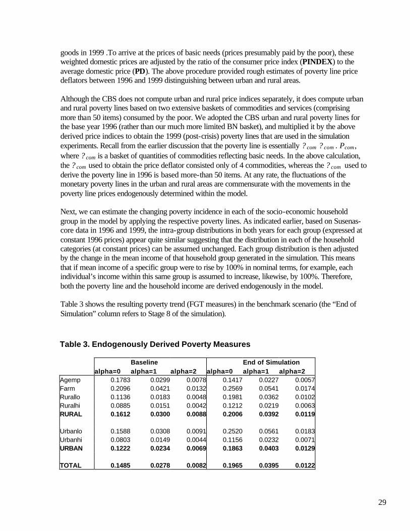
Results from the simulation also indicate that the unemployment increases quite considerably. Yet, the allowance of wage decline and mobility of labor (from urban to rural areas, and from formal to informal sector), a prominent signs of flexible labor market, prevented an even more catastrophic situation from occurring. While during the peak of the crisis the unemployment rate may have increased significantly, towards the end of 1998 and early 1999 the recorded unemployment rate show only a slight increase from the pre-crisis level. Indeed, from the model simulation the increase of unemployment is rather surprisingly small (less-than 1 percentage point). Nonetheless, the combined forces of unemployment, declining real wages (incomes), and a surging poverty price have raised the poverty incidence. There is some evidence of consumption smoothing that led to a poverty incidence lower than originally predicted.22 Also, as the poverty price and the CPI dropped in the later stage (Stage 8), the poverty line declined, and so did the head-count index. In order to attempt to estimate the poverty implications of the above described shocks, we can return to a discussion of the Beta function. Applying such a function (described in section II) to the actual intra-group distributions in the base (1996) year as shown in Figures 2a-2i, one can approximate and fit the parameters corresponding to the characteristics of the different groups. In this report, however, we estimate the poverty incidence based on a parametric measure of distribution, in which the intra-group distribution is directly generated from the Susenas-core data with 206,597sample size. Note that since the Susenas-core does not distinguish between Farmers according to different land sizes (small, medium and large land owners are lumped together), we have to use only six, instead of eight, household categories in the analysis: four in the rural areas, i.e., Agricultural Employee (Agemp), Farmers with land (Farm), Non-farm rural low income household (Rurallo), Non-farm rural high income household (Ruralhi), and two in the urban areas, i.e., Low income urban household (Urbanlo), and High income urban household (Urbanhi). Also, it is important to note that the Susenas survey reflects the conditions in around March of the respective year. It is important to note that the Indonesian Central Bureau of Statistics (CBS) does not produce separate price indices for urban and rural areas. Therefore, in order to come up with estimates of urban and rural poverty we had to generate these price indices. The starting point is to select a basket of Basic Needs (BN) reflecting the consumption pattern of the households around the presumed poverty line and yielding the threshold caloric requirements. Of course food is by far the most important commodity in this BN basket. In our modeling, we limited this basket to only four commodities, i.e., food (rice), other food, textiles, and social services. First, we approximated the consumption share of each of these goods in the base year (1996) BN consumption value for both urban and rural areas (the share of food in the rural BN basket is higher than in the urban BN basket). Next, we computed the weighted average of the BN basket in 1999 keeping the shares constant but using the prices generated endogenously by our model for the four 22 Many households have either changed their food menu (e.g., eating rice once a day, using other less desirable foods the rest of the time), switched to lower price food (e.g., from imported to domestic produce), or used their accumulated savings to purchase food (dis -saving). There is widespread evidence showing that a smoothing process also takes place in non-food consumption. But the impact on poverty, more particularly on diets, is less serious compared to the case when the smoothing is in food consumption (especially among the poor). It is also important to note that the economic crisis was not the only culprit. During 1997/98, Indonesia also suffered from crop failures due to the fickle global weather (El-Nino) phenomenon and a missive haze problem. Subsistence farming areas were the worst affected.

29

goods in 1999 .To arrive at the prices of basic needs (prices presumably paid by the poor), these weighted domestic prices are adjusted by the ratio of the consumer price index (PINDEX) to the average domestic price (PD). The above procedure provided rough estimates of poverty line price deflators between 1996 and 1999 distinguishing between urban and rural areas. Although the CBS does not compute urban and rural price indices separately, it does compute urban and rural poverty lines based on two extensive baskets of commodities and services (comprising more than 50 items) consumed by the poor. We adopted the CBS urban and rural poverty lines for the base year 1996 (rather than our much more limited BN basket), and multiplied it by the above derived price indices to obtain the 1999 (post-crisis) poverty lines that are used in the simulation experiments. Recall from the earlier discussion that the poverty line is essentially ? com ? com . Pcom , where ? com is a basket of quantities of commodities reflecting basic needs. In the above calculation, the ? com used to obtain the price deflator consisted only of 4 commodities, whereas the ? com used to derive the poverty line in 1996 is based more-than 50 items. At any rate, the fluctuations of the monetary poverty lines in the urban and rural areas are commensurate with the movements in the poverty line prices endogenously determined within the model. Next, we can estimate the changing poverty incidence in each of the socio-economic household group in the model by applying the respective poverty lines. As indicated earlier, based on Susenas-core data in 1996 and 1999, the intra-group distributions in both years for each group (expressed at constant 1996 prices) appear quite similar suggesting that the distribution in each of the household categories (at constant prices) can be assumed unchanged. Each group distribution is then adjusted by the change in the mean income of that household group generated in the simulation. This means that if mean income of a specific group were to rise by 100% in nominal terms, for example, each individual’s income within this same group is assumed to increase, likewise, by 100%. Therefore, both the poverty line and the household income are derived endogenously in the model. Table 3 shows the resulting poverty trend (FGT measures) in the benchmark scenario (the “End of Simulation” column refers to Stage 8 of the simulation). Table 3. Endogenously Derived Poverty Measures Baseline End of Simulation alpha=0 alpha=1 alpha=2 alpha=0 alpha=1 alpha=2 Agemp 0.1783 0.0299 0.0078 0.1417 0.0227 0.0057 Farm 0.2096 0.0421 0.0132 0.2569 0.0541 0.0174 Rurallo 0.1136 0.0183 0.0048 0.1981 0.0362 0.0102 Ruralhi 0.0885 0.0151 0.0042 0.1212 0.0219 0.0063 RURAL 0.1612 0.0300 0.0088 0.2006 0.0392 0.0119 Urbanlo 0.1588 0.0308 0.0091 0.2520 0.0561 0.0183 Urbanhi 0.0803 0.0149 0.0044 0.1156 0.0232 0.0071 URBAN 0.1222 0.0234 0.0069 0.1863 0.0403 0.0129 TOTAL 0.1485 0.0278 0.0082 0.1965 0.0395 0.0122

30

It is clear that the deterioration in the poverty conditions is more severe in the urban than in the rural areas. While the head-count poverty among farmers owning land increases from 21 to 26 percent, and among rural non-farm households the increase is from 11 to 20 percent (for low income rural) and from 9 to 12 percent (for high income rural), the poverty incidence within the category of agricultural workers drops from 18 to 14 percent. This last result, although surprising, might be explained by the fact that most agricultural workers are employed in the plantation export sector that benefited from the currency depreciation. In contrast, in the two categories of urban households the head-count poverty incidence increases, most dramatically among the urban low income, i.e., from 16 to 25 percent. Similar trends are observed for the poverty gap and the severity of poverty indicators. Overall, urban poverty appeared to rise from 12% in 1996 to 19% in 1999 and rural poverty from 16% to 20%. From the analysis of the poverty trend, therefore, one can surmise that the crisis has hit the urban households more negatively than the rural households. This result is the combined outcome of two forces, a lower increase in the households’ nominal income and a faster increase in the poverty line price indices in the urban areas than in the rural areas. IV.2 Counterfactual Scenarios Two sets of counterfactuals are conducted: 1) a scenario of maintaining a level of interest rate lower than under the actual benchmark IMF sponsored policy, labeled “Less tight” (for less tight monetary policy); and 2) the same as number 1 but combined with some foreign debt restructuring (labeled “Less tight & debt”). Obviously, these scenarios contrast with the actual or the IMF-style policy discussed earlier (labeled “Benchmark (IMF)”). Since the IMF entry was in November 1997, the starting point of the relevant adjustments to the exogenous variables is in Stage 4. To conduct a proper comparison, the exogenous changes in each stage, except for the interest rate and the level of foreign debt, are kept the same as in the original (benchmark) simulation described in the preceding section.23 In stages 4 to 7, the influence of the political risks (POLRISK) under the two counterfactual scenarios is set lower than in the benchmark simulation. This approach is taken because political and socio-economic repercussions of a more reasonable level of interest rate are expected to be less severe.24 Indeed, the political situation worsened between January and May 1998 (between stage 5-food riots and beginning of bankruptcies-and stage 6-May riots culminating in the fall of Suharto). The model contains a set of relationships where exchange rate expectations are determined indirectly through POLRISK variable. Although this variable is set exogenously, not

23 When the interest rate is set lower, the decline in the banking sector should have also been lower (e.g., less bankruptcy). The size of the resulting depressed construction sector, being the most bank-sensitive activity, would also be affected subsequently. In the two counterfactuals, we accommodate such changes in the relevant stages where downward adjustments have been imposed under the benchmark simulation. 24 When the interest rate surged, the probability of more bankruptcies became higher. Furthermore, the unfavorable impact on output dragged domestic investment further down, causing more severe repercussions on the economy. At some stage, the political environment and uncertainty could have been further jeopardized. Hence, under the two counterfactuals, the POLRISK exogenous variable would have been lower than in the “Benchmark (IMF)” scenario.

31

functionally linked to specific events, most objective observers would agree that this variable worsened considerably during the first half of 1998 yielding the conditions prevailing under the actual “Benchmark (IMF)” scenario. It can be argued, therefore, that under the two alternative counterfactual scenarios a less tight monetary policy resulting in lower interest rates would have led to a milder recession and a less unfavorable political situation. This is reflected in the model by using a less extreme value of POLRISK in the two counterfactual scenarios than in the benchmark scenario. The second counterfactual experiment, labeled “Less tight & debt,” is to combine a fixed interest rate with a partial resolution of the foreign debts. This is done by lowering DEBSERV in Stages 4 and 5, that will cause RISK variable to decline, and consequently PFCAPIN to increase (see equations 1 and 2). Figure 18 shows the assumed trend of interest rate under the aforementioned three scenarios. Figures 19 to 24 depict the resulting trajectories of net flows, real GDP, income distribution index, price index, poverty-line prices, and the exchange rate. Since the different shocks are applied starting at Stage 4, these Figures show only the trends from Stage 4 to Stage 8.

Figure 18. Interest Rate Scenarios

0

0.2

0.4

0.6

0.8

1

1.2

1.4

Stage 4 Stage 5 Stage 6 Stage 7 Stage 8

Inde

x

Benchmark (IMF)

Less tight

Less tight & debt

32

Figure 19. Net Capital Flows: Benchmark & Counterfactuals

0.9

0.95

1

1.05

1.1

1.15

1.2

1.25

1.3

Stage 4 Stage 5 Stage 6 Stage 7 Stage 8

Ind

ex

Benchmark (IMF)Less tightLess tight & debt

Figure 20. Real GDP: Benchmark & Counterfactuals

0.85

0.9

0.95

1

1.05

Stage 4 Stage 5 Stage 6 Stage 7 Stage 8

Inde

x

Benchmark (IMF)Less tightLess tight & debt

33

Figure 21. Income Distribution: Benchmark & Counterfactuals

0.98

1.03

1.08

1.13

1.18

Stage 4 Stage 5 Stage 6 Stage 7 Stage 8

Inde

x

Benchmark (IMF)Less tightLess tight & debt

Figure 22. Prices: Benchmark & Counterfactuals

1

1.1

1.2

1.3

1.4

1.5

1.6

1.7

1.8

1.9

2

Stage 4 Stage 5 Stage 6 Stage 7 Stage 8

Ind

ex

Benchmark (IMF)Less tightLess tight & debt

34

Figure 23. Prices for Poverty Line: Benchmark & Counterfactuals

1

1.1

1.2

1.3

1.4

1.5

1.6

1.7

1.8

1.9

Stage 4 Stage 5 Stage 6 Stage 7 Stage 8

Ind

ex

Benchmark (IMF)Less tightLess tight & debt

Figure 24. Exchange Rates: Benchmark & Counterfactuals

1

1.1

1.2

1.3

1.4

1.5

1.6

1.7

1.8

1.9

2

Stage 4 Stage 5 Stage 6 Stage 7 Stage 8

Ind

ex

Benchmark (IMF)Less tightLess tight & debt

35

Under the two alternative scenarios, the impact on output (real GDP) and prices is more favorable than in the “Benchmark (IMF)” scenario. While a higher interest rate produces an output-curtailment effect, the corresponding depreciation of the exchange rate appears to be even worse. The latter is formed through the following mechanisms. As the domestic investment (DOMPI) drops, domestic output, D, and exports, E, are adversely affected, causing GDP to decline and the RISK factor to rise. In turn, this reduces private capital inflows, PFCAPIN. The higher RISK also pushes the expected exchange rate, EXPEXR, to surge, resulting in severe depreciation of the rupiah. Hence, despite the standard mechanism of the interest parity equation, the intended impact of a high interest rate is offset by a rise in EXPEXR through the above channel, causing greater depreciation of the exchange rate. The above mechanism is repeated and reinforced by the presence of the Bernanke-Gertler-Krugman effects of the exchange rate on investment. As shown in Figure 20, the high and non-high interest rate policy could result in a difference of real GDP as much as 5.7% for the entire Stage 4-Stage 8 period. In Stage 8 alone the gap could be as high as 9.6%. Meanwhile, the exchange rate under the non-high interest rate scenario would have been stronger by between 3.9 to 5.5%. (Figure 24). With identical POLRISK under the “Less tight” and “Less tight & debt,” the exchange rate appears stronger in the latter. As stated in Section III, the recorded data show that during the crisis the unemployment rate increased by “only” less-than one percentage point (around .8 percent according to Sakernas), suggesting a fairly high degree of flexibility in the country’s labor markets. Indeed, the benchmark scenario generated by the model also points to a small increase of the unemployment rate. However, from the perspectives of counterfactuals, the unemployment rate under the “Benchmark (IMF)” scenario is still highest among the three, a result that is consistent with the GDP trend. As an illustration, in Stage 8, the unemployment rate in the “Less tight” experiment is considerably lower than (around half of) the rate under the benchmark scenario. In terms of net capital flows, there is a fluctuating trend, but “Less tight” is always superior to the other two scenarios (Figure 19). The reason why it produces greater inflows than in “Less tight & debt” is because, with a debt rescheduling the new inflows appear to be much smaller than with no debt rescheduling (any debt resolution tends to deter further inflows), although the outflows are larger in the latter. At this juncture, it is important to stress that the length of the period covered in the sequential simulations is rather limited. The positive effects of a debt resolution (e.g., on exchange rate) may not be immediately felt; it would probably emerge only beyond Stage 8. The generated income distribution is rather interesting. Up to Stage 5, all scenarios produce an improvement. But in the subsequent stages, there is clearly a worsening trend of income distribution (Figure 21). The resulting difference between “Less tight” and “Less tight & debt” is small, but still favoring the latter, e.g., 1.45 versus 1.43. It is revealing that there is a close correlation between worsening (improving) trend of income distribution and increasing (lowering) interest rate. Surely, the interest incomes and the windfall from foreign asset holding (e.g., time deposit in foreign currency) under the environment of super-high interest rate and severe collapse of the exchange rate have contributed to such a relation.

36

Nevertheless, the relative income distribution under the “Benchmark (IMF)” is clearly the least preferable one; it is persistently worst among the three scenarios. Recall that the inequality measure used in this study is derived from the mean incomes of the 8 household groups. Each intra-group distribution is assumed to remain the same as in the base (1995/6) period. Yet, in the present context, this is a defensible assumption, as a comparison of the actual pre- and post-crisis group distributions in Figs.2a-2i suggest. The numerical effects of the scenarios on prices show that up to Stage 7 the “Benchmark (IMF)” produces the highest price index. The gap is largest in Stage 6, though prices are converging in the remaining stages. In fact, in Stage 8 both the price level and the poverty line price level under the “Benchmark (IMF)” is slightly lower than under the “Less tight” scenario (Figures 22 and 23). Nonetheless, for the entire period the poverty line price level is still highest under the “Benchmark (IMF)” experiment. We are, therefore, of the opinion that not only the macroeconomic indicators but also the poverty conditions would have been better if the country had not been stuck too rigidly with the IMF-style policy. The above counterfactual experiments clearly demonstrate that the policy scenario of not raising the interest rate would have created potential benefits in terms of macroeconomic indicators as well as social indicators. Furthermore, with the only exception of net capital flows, the results generated from the combination of non-high interest rate and partial debt resolution at the early stages of the crisis appear to be the most preferred. V. Closing Remarks The main objective of the model was to incorporate the various channels and transmission mechanisms through which the Asian Financial Crisis and political instability affected the socio-economic system and, ultimately, poverty in Indonesia during the period 1997-1999. Hence, the model contains a detailed financial sector and a poverty module. Three of the transmission mechanisms were triggered by the initial outflow of capital following the contagion effects of the Thai crisis in July 1997. The outflow of capital led to pressures on the exchange rate and fueled expectations of further depreciations. In turn, the impact of the worsening exchange rate affected the socio-economic system through three different channels: (1) a drop in the domestic investment, the so-called Bernanke-Gertler-Krugman effect; (2) a rise in the price level (mainly through higher import prices) which was further magnified by unfavorable weather conditions and a drop in agricultural output; and (3) a higher cost of imported intermediate inputs that dampened domestic output. The combined effects of these three mechanisms were to reduce aggregate demand and supply. The depreciation of the exchange rate also affected consumption and poverty incidence negatively through its impact on the price level. Along with the high interest rate policy, this also worsened the relative income distribution. In addition, the crisis was further propagated through the following financial mechanisms: (1) the pessimistic expectation relative to the exchange rate and the political instability induced agents to reallocate their wealth portfolios away from domestic assets towards foreign assets--reducing thereby the flows of demand and time deposits and the supply of loanable funds; and (2) the

37

relatively high interest rate (particularly under the IMF-sponsored policy) led to a credit crunch, deteriorating balance sheet, bankruptcies, and further stagnation of domestic investment.

38

Appendix 1

Cumulative Density Functions for Different Household Groups, 1996 and 1999 at Constant 1996 Prices

Figure 1a: Agricultural Worker

0 1 2 3 4 5 6 7 8 9 10 11 12 13 14

x 105

0

0.1

0.2

0.3

0.4

0.5

0.6

0.7

0.8

0.9

1

Income (Rupiah)

Po

pu

lati

on

In

de

x

Agricultural Workers

9699

Figure 1b: Farmers with Land

0 0.2 0.4 0.6 0.8 1 1.2 1.4 1.6 1.8 2

x 106

0

0.1

0.2

0.3

0.4

0.5

0.6

0.7

0.8

0.9

1

Income (Rupiah)

Pop

ulat

ion

Inde

x

Farmers w/Land

9 69 9

39

Figure 1c: Rural Low

0 2 4 6 8 10 12 14 16 18

x 105

0

0.1

0.2

0.3

0.4

0.5

0.6

0.7

0.8

0.9

1

Income (Rupiah)

Pop

ulat

ion

Inde

x

Rural Low

9699

Figure 1d: Rural Non-Labor Force

0 0.2 0.4 0.6 0.8 1 1.2 1.4 1.6 1.8 2

x 106

0

0.1

0.2

0.3

0.4

0.5

0.6

0.7

0.8

0.9

1

Income (Rupiah)

Pop

ulat

ion

Inde

x

Rural Non-LbF

9699

40

Figure 1e: Rural High

0 0.3 0.6 0.9 1.2 1.5 1.8 2.1 2.4 2.7 3

x 106

0

0.1

0.2

0.3

0.4

0.5

0.6

0.7

0.8

0.9

1

Income (Rupiah)

Pop

ulat

ion

Inde

x

Rural High

9699

Figure 1f: Urban Low

0 0.3 0.6 0.9 1.2 1.5 1.8 2.1 2.4 2.7 3 3.3 3.6 3.9

x 10 6

0

0.1

0.2

0.3

0.4

0.5

0.6

0.7

0.8

0.9

1

Income (Rupiah)

Pop

ulat

ion

Inde

x

Urban Low

9699

41

Figure 1g: Urban Non-Labor Force

0 0.3 0.6 0.9 1.2 1.5 1.8 2.1 2.4 2.7 3

x 10 6

0

0.1

0.2

0.3

0.4

0.5

0.6

0.7

0.8

0.9

1

Income (Rupiah)

Pop

ulat

ion

Inde

xUrban Non-LbF

9699

Figure 1h: Urban High

0 0.3 0.6 0.9 1.2 1.5 1.8 2.1 2.4 2.7 3 3.3 3.6 3.9 4.2 4.5

x 10 6

0

0.1

0.2

0.3

0.4

0.5

0.6

0.7

0.8

0.9

1

Income (Rupiah)

Pop

ulat

ion

Inde

x

Urban High

9699

42

Figure 1i: Rural Groups

0 0.2 0.4 0.6 0.8 1 1.2 1.4 1.6 1.8 2

x 10 6

0

0.1

0.2

0.3

0.4

0.5

0.6

0.7

0.8

0.9

1

Income (Rupiah)

Pop

ulat

ion

Inde

xRural Groups

9699

Figure 1j: Urban Groups

0 0.3 0.6 0.9 1.2 1.5 1.8 2.1 2.4 2.7 3 3.3 3.6 3.9

x 10 6

0

0.1

0.2

0.3

0.4

0.5

0.6

0.7

0.8

0.9

1

Income (Rupiah)

Pop

ulat

ion

Inde

x

Urban Groups

9699

43

Intra-Group Distributions, 1996 and 1999 at Constant 1996 Prices

Figure 2a: Agricultural Workers

Note: Top figure (1996), Bottom figure (1999)

2 3 4 5 6 7 8 9 10 11

x 10 5

0

50

100

Pop

ulat

ion

(Per

son)

Agricultural Workers

2 3 4 5 6 7 8 9 10 11

x 10 5

0

50

100

Pop

ulat

ion

(Per

son)

Expenditure per Person (Rp)

44

Figure 2b: Farmers with Land

2 4 6 8 10 12 14 16 18

x 10 5

0

200

400

600

800 P

opul

atio

n (P

erso

n)

Farmers w/Land

2 4 6 8 10 12 14 16 18

x 10 5

0

200

400

600

800

Pop

ulat

ion

(Per

son)

Expenditure per Person (Rp)

45

Figure 2c: Rural Low

2 4 6 8 10 12 14 16

x 10 5

0

50

100

150

200

250

Pop

ulat

ion

(Per

son)

Rural Low

2 4 6 8 10 12 14 16

x 10 5

0

50

100

150

200

250

Pop

ulat

ion

(Per

son)

Expenditure per Person (Rp)

46

Figure 2d: Rural Non-Labor Force

2 4 6 8 10 12 14 16

x 10 5

0

50

100

Pop

ulat

ion

(Per

son)

Rural Non-LbF

2 4 6 8 10 12 14 16

x 10 5

0

50

100

Pop

ulat

ion

(Per

son)

Expenditure per Person (Rp)

47

Figure 2e: Rural High

2 4 6 8 10 12 14 16

x 10 5

0

50

100

Pop

ulat

ion

(Per

son)

Rural High

2 4 6 8 10 12 14 16

x 10 5

0

50

100

Pop

ulat

ion

(Per

son)

Expenditure per Person (Rp)

48

Figure 2f: Urban Low

0.2 0.4 0.6 0.8 1 1.2 1.4 1.6 1.8 2 2.2

x 10 6

0

50

100

150

200

Pop

ulat

ion

(Per

son)

Urban Low

0.2 0.4 0.6 0.8 1 1.2 1.4 1.6 1.8 2 2.2

x 10 6

0

50

100

150

200

Pop

ulat

ion

(Per

son)

Expenditure per Person (Rp)

49

Figure 2g: Urban Non-Labor Force

0.2 0.4 0.6 0.8 1 1.2 1.4 1.6 1.8 2

x 10 6

0

50

100

Pop

ulat

ion

(Per

son)

Urban Non-LbF

0.2 0.4 0.6 0.8 1 1.2 1.4 1.6 1.8 2

x 10 6

0

50

100

Pop

ulat

ion

(Per

son)

Expenditure per Person (Rp)

50

Figure 2h: Urban High

0.2 0.4 0.6 0.8 1 1.2 1.4 1.6 1.8 2

x 10 6

0

50

100

150

200

250

Pop

ulat

ion

(Per

son)

Urban High

0.2 0.4 0.6 0.8 1 1.2 1.4 1.6 1.8 2

x 10 6

0

50

100

150

200

250

Pop

ulat

ion

(Per

son)

Expenditure per Person (Rp)

51

Figure 2i: Rural Groups

2 4 6 8 10 12 14 16

x 105

0

500

1000

1500

Pop

ulat

ion

(Per

son)

Rural Groups

2 4 6 8 10 12 14 16

x 105

0

500

1000

1500

Pop

ulat

ion

(Per

son)

Expenditure per Person (Rp)

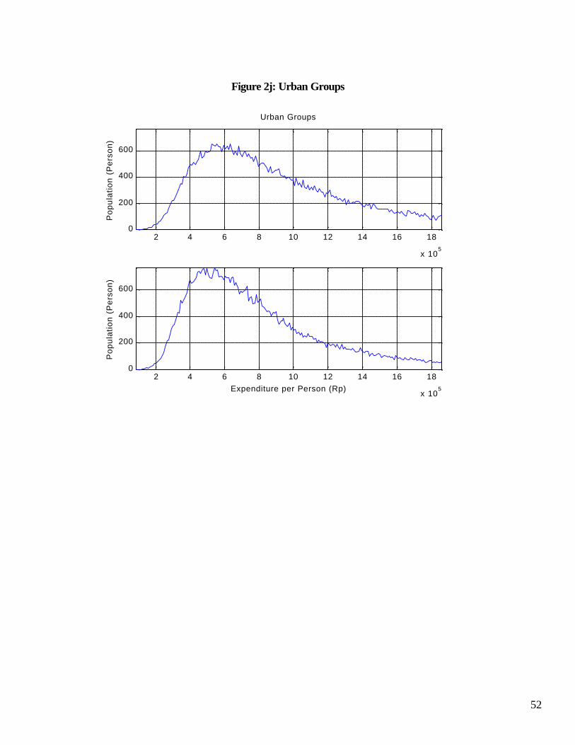
52

Figure 2j: Urban Groups

2 4 6 8 10 12 14 16 18

x 105

0

200

400

600

Pop

ulat

ion

(Per

son)

Urban Groups

2 4 6 8 10 12 14 16 18

x 105

0

200

400

600

Pop

ulat

ion

(Per

son)

Expenditure per Person (Rp)

53

APPENDIX 2. LIST OF EQUATIONS IN THE CGE MODEL OUTPUT SUPPLY AND FACTOR DEMAND Xp = axp . [ ? p.VAp ? p? + (1-? p). INTMp

-? p ] -1/? p (1) VAp = avp . [? f ? p,f .FACDEMp,f

??p] -1/?p (2)

FACDEMp,f = VAp . [? p,f . PVp / (av?p. WFf . WFDISTp,f)] 1/(1+?p) (3) INTMp = VAp / [ (PINTMp/PVp). (? p/(1-? p)) ] 1/(1 + ? p) (4) INTMp = abp.? btp. DOMINTp

-?p + (1-btp). FORINTp-?p?(1/?p) (5)

FORINTMp = DOMINTp . PDINTMp/PFINTMp . ((1-btp)/btp)1/(1+?p) (6) Xp = ATp . ( ?p.Ep

?p + (1-?p ).Dp?p) 1/?p

p? pexp (7) Xp = Dp p? pexp (8) Ep = Dp . [ PEp/ (PDp(1-tdomp-ttdp)) . (1-?p)/?p ] 1/(?p-1) p? pexp (9) Qp = acp . [? p.Mp

??p +(1-? p).Dp-?p] -1/?p p? pimp (10)

Qp = Dp p? pimp (11) Mp = Dp . [ (PDp/PMp) . ? p / (1-? p) ] 1/(1 + ?p) p? pimp (12) AGGREGATE DEMAND XINTQp = ? pp(aadp,pp .PDINTMpp.DOMINTpp + aamp,pp .PFINTMpp.FORINTMpp)/PQp (13) HHCONQp = [ ? ihh alphqp,ihh .(1-mpsihh).YCONSihh ] / PQp (14) GCp = gconsqp.GTOT (15) IDp = ? pp (capmatp,pp . DKpp.PKpp )/PQp (16) INVENp = invp . Xp (17) PRICES PXp = [PDp.Dp(1-tdomp-ttdp) + PEp.Ep ] / Xp (18) PQp = [ PDp.Dp + PMp.Mp ] / Qp (19) PVp = [ PXp.Xp - PINTMp .INTMp ] / VAp (20) PKp = ? pp {capmatpp,p .PQpp } (21) PMp = pwmp.EXR . (1 + tmp+ttip) (22) PEp = pwep . EXR (23) PDINTMp = ? pp { aadpp,p . PDpp } (24) PDINTMp = ? pp { aampp,p . PMpp } (25) PINTMp = ? PDINTMp.DOMINTMp + PFINTMp.FORINTMp? / INTMp (26) PINDEX = ? i wtqp.PQp (27) PINDOM = ? p wtdp.PDp (28)

54

INCOME AND SAVING YFf = ? p (WFf . WFDPSTp,f . FACDEMp,f ) f?capital (29) YFcapital = WFcapital . ? p ( WFDISTp,capital . FACDEMp,capital ) - EXR.REPAT - ? hfin ( RT . OTDHhfin + RFLOAN . EXR . OTFHhfin ) YCORP = factoincompny,capital .YFcapital - EXR. DEBSERVcompany (30) YCONSihh = YHHihh. .(1 - thihh).(1- mpsihh -? ihh transihhihh,ihhh ) (32) HHSAV = ? ihh mpsihh .YHHihh .(1 - thihh) (33) INDTAX = ? p (tdomp.PDp.Dp + tmp.pwmp.EXR.Mp ) (34) TTMTOT = ? p (ttdp.PDp.Dp + ttip.pwmp.EXR.Mp ) (35) GOVREV = INDTAX+? ihh thihh .YHHihh + YCORP . ctax + factoingovt,capital.YFcapital (36) GOVEXP = ? p PQp.GCp + EXR . DEBTSERVgovt + GTRANTOT + BONDS + RBONDS (37) GOVSAV = GOVREV - GOVEXP (38) CORSAV = YCORP . (1 - ctax) .?????ihh compdistihh ) (39) FSAV = -(? p pwep.Ep -?? p pwmp.Mp +? ihh ROWTRANihh - REPAT - FOREXDEB ) (40) SAVING = HHSAV + GOVSAV + CORPSAV + EXR.FSAV (41) LABOR MARKET WAGESp = PINDEX?p/1.5. (PVp/PV0p)(1-?p) . (Xp/? fl FACDEMp,fl /PDL0p)?p (42) WFfl = WF0fl .? p WAGESp .wsharep,fl (43) DFLfl= Sp FACDEMP\p,fl (44) ? fflMIGfl,ffl= ? ffl LS0fl.? ?0fl ?(DFLfl/DFL0fl)/(DFLffl/DFL0ffl)??2fl-1fl,ffl? (45) ? fflMIGffl,fl=? flMIGffl,fl (45a) LSfl = LS0fl.(1+lgrowfl) + ? ffl MIGfl,ffl (46) INVESTMENT AND CAPITAL FLOWS PFCAPIN = ? 0 +degree.? ?.(RLOAN-RFLOAN-RISK/scal) (47) RISK = ? 0 + ? 1. FOREXDEB / ? pEp .pwep ) (48) FOREXDEB = ? inl DEBSERVinl (49) FORINVNET = FCAP -? ?inl BORROWinl (50) FORINVp = fpinvp. FORINVNET (51) FCAP = PFCAP + BORROWgovt (52) DFR = FSAV - FCAP + ? ihh HHFRihh (53) DOMPINVp = ? p.VAp

?1p.(1+RLOAN)??p.EXR?3 (54)

PINVp = DOMPINVp + EXR . FORINVp (55) DKp = ( GOVINVp + PINVp )/PKp (56) TOTINVEST =?? p (GINVp+ PINVp) (57) PFCAP = PFCAPIN – PFCAPOUT (58) PFCAPOUT = ? o . (PEQ.EQROW/EXR)?1 (59) PEQ.EQROW = OEQROW + EXR.FORINVNET (60)

55

REAL SECTOR MARKET CLEARING Qp = XINTQp+HHCONQp+GCp+IDp+ INVENp +ttindpTTMTOT/PQp (61) FSf = ? p FACDEM p,f (62) SAVING = TOTINVEST (63)* GDP = ? p?PVAp.VAp + INDTAX (64) LSfl = ? p FACDEMp,fl + UNEMfl (65) Note * Eq (63) is not included in the body of the model; When the model is fully specified, this condition is fulfilled according to Walras Law INSTITUTION SAVINGS YBANK = RLOAN.? pOBANKLOANp + RSBI.OSBI - RT.( ? ihhOTDHihh + ? pOTDIp + OTDGOV) - RFLOAN.EXR. (? ihhOTFHihh + ? pOTFIp) (66) BANKSAV = cmsav.YBANK + BONDS + RBONDS (67) FIRMSAV = CORSAV - BANKSAV (68) (1-rrgov).BORROWgovt = (? pGOVINVp - GOVSAV)/EXR (69) INTEREST RATES RT = RLOAN - RGAP (70) RAVG = (RT.(? ihhTDHihh + ? pTDIp + TDGOV) + RFLOAN.EXR.(? ihhTFHihh))/ (? ihh(TDHihh + EXR0.TFHihh) ) (71) RQ = ?YFcapital + ? ihh (RT.OTDHihh + RFLOAN.EXR.OTFHihh) + EXR.REPAT - RLOAN.? p (BANKLOANp + CBLOANp) - RFLOAN.EXR. ? p (OROWLOANp + ROWLOANp)? / PEQ.? p EQF (72) RWAVG = frow . RFLOAN + (1-frow).EXR0.RQ/EXR (73) RLOAN = RFLOAN + (EXPEXR/EXR -1) + POLRISK (74) INSTITUTION PORTFOLIO MDHihh = bmh0ihh.YDISPihh

bmh1ihh.e(RAVG.bmh2ihh).PINDEX (75) tdcur = (? ihh( TDHihh+ TFHihh) + ? p (TDIp+TFIp ))/CURRENCY (76) RM = BANKRES + CURRENCY (77) CURRENCY = ? ihh curatihh. MDHihh (78) MDIp = gf1p.PXp.Xp (79) gh1hfin/(1 - gh1hfin) = phih1hfin.((1 + RAVG)/(1 + RQ))epsh1hfin (80) gh2hfor/(1 - gh2hfor) = phih2hfor.((1 + RT)/(1 + RFLOAN + (EXPEXR-EXR0)/EXR0))epsh2hfor(81) TDHihh = gh2ihh.gh1ihh.(WEALHihh - MDHihh - EXR.HHFRihh (82) TDIp = gdip.BANKLOANp (83) TFHihh = (1 - gh2ihh).gh1ihh.(WEALHihh - MDHihh - EXR.HHFR)/EXR (84) TFIp = gf2p. (OROWLOANp + ROWLOANp) (85) PEQ.EQHihh = (1 - gh1ihh)(WEALHihh - MDHihh - EXR.HHFRihh) (86) EQROW = OEQROW + FORINVNET/PEQ (87) frow/(1 - frow) = phirow.((1 + RW)/(1 + RQ - EXR/EXR0))epsrow (88)

56

FORINVNET = (1 - frow).PFCAP (89) PFBORROW = frow.PFCAP (90) frow/(1-frow) = phirow. ?(1+RFLOAN + (EXPEXR - EXR0)/EXR0)/(1+RQ)?epsrow (91) fb2/(1 - fb2) = phib2.((1 + RLOAN)/(1 + RW + (EXR-EXR0)/EXR0))epsb2 (92) BORROWcombank = WEALROW + CBFR + ? ihh HHFRihh - ? inl OBORROWinl - BORROWgovt ? p (OROWLOANp + ROWLOANp) - PEQ.EQROW/EXR (93) BORROWcombank = bankbor. PFBORROW (94) ROWLNTOT = (1-bankbor). PFBORROW (95) ROWLOANp = rowsharep.ROWLNTOT (96) INSTITUTION WEALTH WEALHihh = mpsihh.YHHihh.(1 - thihh) + OWEALHihh + (EXR - EXR0).OTFHihh + (PEQ - PEQ0).OEQH (97) WEALBANK = BANKSAV + OWEALBANK - (EXR-EXR0).?OBORROWcombank + ? ihhOTFHihh + ? pOTFIp) (98) WEALCB = OWEALCB + (EXR - EXR0).OCBFR (99) WEALGOV = GOVSAV + OWEALGOV - (EXR - EXR0).OBORROWgovt + (PEQ - PEQ0).OEQGOV (100) WEALROW = OWEALROW + FSAV + (PEQ/EXR - PEQ0/EXR0).OEQROW -(1-EXR0/EXR).(OCBFR-? inlOBORROWinl-? pOROWLOANp (101) WEALFIRM = OWEALFIRM + FIRMSAV + (PEQ - PEQ0).OEQFIRM (102) INSTITUTION FINANCIAL CONSTRAINTS BANKRES = resd.(dcur.CURRENCY) + rest.(? ihh(TDHihh + EXR.TFHihh) + ? p(TDIp + EXR.TFIp) + TDGOV) (103) BANKF + SBI + BANKRES + BONDS + RBONDS = WEALBANK + dcur.CURRENCY + ? ihh(TDHihh + EXR.TFHihh) + ? p(TDIp + EXR*TFIp) + TDGOV +

EXR.(1-rrbank). (OBORROWcombank +BORROWcombank) + CBTRAN (104) BANKF = (1-bb1)* ?WEALBANK + dcur.CURRENCY + ? ihh(TDHihh + EXR.TFHihh) +

? p(TDIp + EXR*TFIp) + TDGOV + EXR.(1-rrbank).(OBORROWcombank + BORROWcombank) - BANKRES + CBTRAN? (105) bb1 = brow1.((1+rsbi*adp)/(1+rloan))brow2 (106) BANKLOANp = lnsharep.BANKF (107) CBLOANp = cbsharep. CBLNTOT (108) RM = CBLNTOT + CBTRAN + EXR. CBFR - WEALCB - DDGOV – SBI (109) RM = BANKRES + CURRENCY + rrbank.EXR.(OBORROWcombank+BORROWcombank) + rrgov.EXR.(OBORROWgovt+BORROWgovt) + ? p rrsecp.(OROWLOANp

+ROWLOANp) (110) M2D = ? ihh (MDHihh + TDHihh + EXR.TFHihh) + ? p (MDIp + TDIp + EXR.TFIp) (111) MS2 = mult. RM (112) mult = (1+dcur+tdcur)/(1+resd.dcur+rest.tdcur+(rrgov.EXR(OBORROWgovt+BORROWgovt) +rrbank.EXR(OBORROWcombank+BORROWcombank)+rrsecp.EXR.(OROWLOANp

+ROWLOANp)/CURRENCY)) (113) MS2CBFR = MS2/(EXR. CBFR) (114)

57

WEALFIRM = PEQ.EQFIRM (115) WEALGOV + EXR.(1-rrgov).(OBORROWgovt + BORROWgovt) + BONDS + RBONDS = DDGOV + TDGOV + PEQ.EQGOV (116) PEQ.EQFp + BANKLOANp + EXR.(1-rrsecp).(OROWLOANp + ROWLOANp) + CBLOANp +(EXR-EXR0)(OTFI-OROWLOANp) = PKp.FACDEMp,capital + FACDEMp,land + PKp.DKp + MDIp + TDIp + EXR.TFIp + (PEQ-PEQ0).? pOEQFp (117) EQUILIBRIUM IN ASSET MARKET ? pEQFp = ? ihhEQHihh + EQFIRM + EQGOV + EQROW (118) M2D = MS2 (119) INCOME DISTRIBUTION AND POVERTY MODULE YHHihh = ? f factoinihh,f.YFf+EXR*ROWTRANihh+? ihh transihhihh,ihhh .YHHihhh . (1-thhihhh) + gtranihh.GTRANTOT+compdist ihh .(1-ctax).YCORP+ RT.OTDHihh + RFLOAN . EXR . OTFHihh (120) gYihh = YHHihh/YHH0ihh (121) Yshh = Y0shh* gYihh (122) Zu

ihh = u1*Pfood + u2*Pnonfood + u3*Ptextile + u1*Psocsvc (123) Zr

ihh = r1*Pfood + r2*Pnonfood + r3*Ptextile + r1*Psocsvc (124)

? ???

??? ?

?z

ihhihhihhihhihh dyyf

zyz

P0

)(?

? (125)

A) SUBSCRIPTS p,pp Production sectors f Factors of production i Institutions inl Non-labor institution (Government, Company,Commercial Bank) ihh,ihhh Household (HH) categories pexp Export sectors hfin HH with interest-bearing assets hfor HH with foreign currency denominated assets B) VARIABLES OUTPUT SUPPLY AND FACTOR DEMAND Dp SALES OF DOMESTIC OUTPUT Ep EXPORTS Mp IMPORTS INTMp COMPOSITE INTERMEDIATE INPUTS

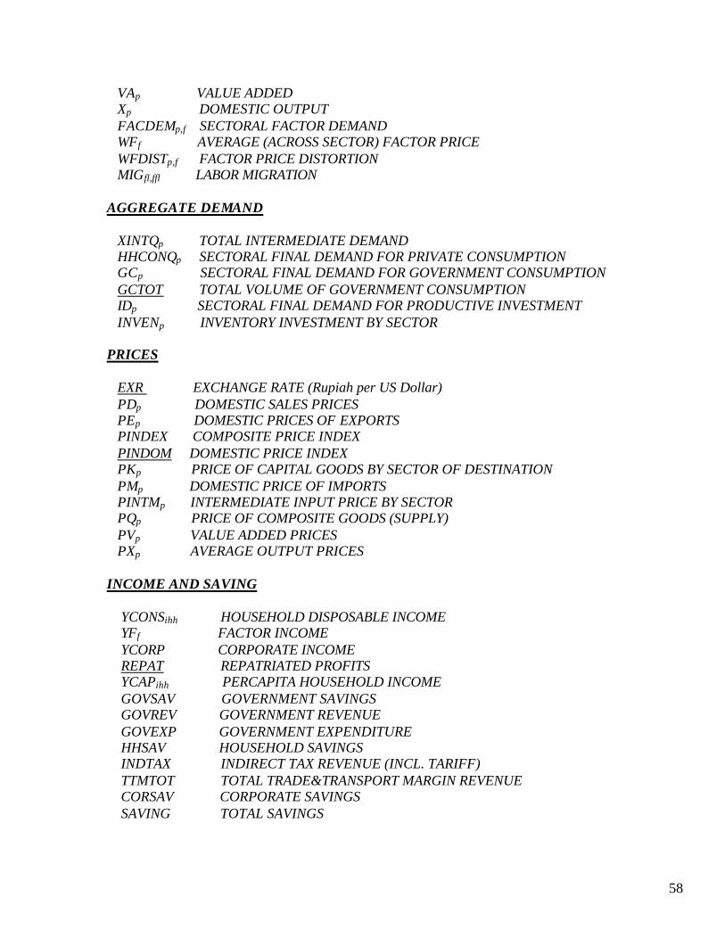
58

VAp VALUE ADDED Xp DOMESTIC OUTPUT FACDEMp,f SECTORAL FACTOR DEMAND WFf AVERAGE (ACROSS SECTOR) FACTOR PRICE WFDISTp,f FACTOR PRICE DISTORTION MIGfl,ffl LABOR MIGRATION AGGREGATE DEMAND XINTQp TOTAL INTERMEDIATE DEMAND HHCONQp SECTORAL FINAL DEMAND FOR PRIVATE CONSUMPTION GCp SECTORAL FINAL DEMAND FOR GOVERNMENT CONSUMPTION GCTOT TOTAL VOLUME OF GOVERNMENT CONSUMPTION IDp SECTORAL FINAL DEMAND FOR PRODUCTIVE INVESTMENT INVENp INVENTORY INVESTMENT BY SECTOR PRICES EXR EXCHANGE RATE (Rupiah per US Dollar) PDp DOMESTIC SALES PRICES PEp DOMESTIC PRICES OF EXPORTS PINDEX COMPOSITE PRICE INDEX PINDOM DOMESTIC PRICE INDEX PKp PRICE OF CAPITAL GOODS BY SECTOR OF DESTINATION PMp DOMESTIC PRICE OF IMPORTS PINTMp INTERMEDIATE INPUT PRICE BY SECTOR PQp PRICE OF COMPOSITE GOODS (SUPPLY) PVp VALUE ADDED PRICES PXp AVERAGE OUTPUT PRICES INCOME AND SAVING YCONSihh HOUSEHOLD DISPOSABLE INCOME YFf FACTOR INCOME YCORP CORPORATE INCOME REPAT REPATRIATED PROFITS YCAPihh PERCAPITA HOUSEHOLD INCOME GOVSAV GOVERNMENT SAVINGS GOVREV GOVERNMENT REVENUE GOVEXP GOVERNMENT EXPENDITURE HHSAV HOUSEHOLD SAVINGS INDTAX INDIRECT TAX REVENUE (INCL. TARIFF) TTMTOT TOTAL TRADE&TRANSPORT MARGIN REVENUE CORSAV CORPORATE SAVINGS SAVING TOTAL SAVINGS

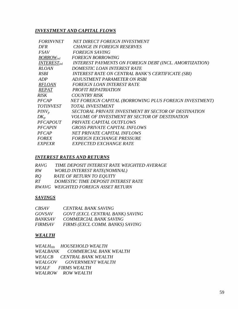
59

INVESTMENT AND CAPITAL FLOWS FORINVNET NET DIRECT FOREIGN INVESTMENT DFR CHANGE IN FOREIGN RESERVES FSAV FOREIGN SAVING BORROWinl FOREIGN BORROWING INTERESTinl INTEREST PAYMENTS ON FOREIGN DEBT (INCL. AMORTIZATION) RLOAN DOMESTIC LOAN INTEREST RATE RSBI INTEREST RATE ON CENTRAL BANK’S CERTIFICATE (SBI) ADP ADJUSTMENT PARAMETER ON RSBI RFLOAN FOREIGN LOAN INTEREST RATE REPAT PROFIT REPATRIATION RISK COUNTRY RISK PFCAP NET FOREIGN CAPITAL (BORROWING PLUS FOREIGN INVESTMENT) TOTINVEST TOTAL INVESTMENT PINVp SECTORAL PRIVATE INVESTMENT BY SECTOR OF DESTINATION DKp VOLUME OF INVESTMENT BY SECTOR OF DESTINATION PFCAPOUT PRIVATE CAPITAL OUTFLOWS PFCAPIN GROSS PRIVATE CAPITAL INFLOWS PFCAP NET PRIVATE CAPITAL INFLOWS FOREX FOREIGN EXCHANGE PRESSURE EXPEXR EXPECTED EXCHANGE RATE

INTEREST RATES AND RETURNS

RAVG TIME DEPOSIT INTEREST RATE WEIGHTED AVERAGE RW WORLD INTEREST RATE(NOMINAL) RQ RATE OF RETURN TO EQUITY RT DOMESTIC TIME DEPOSIT INTEREST RATE RWAVG WEIGHTED FOREIGN ASSET RETURN SAVINGS CBSAV CENTRAL BANK SAVING GOVSAV GOVT (EXCL CENTRAL BANK) SAVING BANKSAV COMMERCIAL BANK SAVING FIRMSAV FIRMS (EXCL COMM. BANKS) SAVING WEALTH WEALHihh HOUSEHOLD WEALTH WEALBANK COMMERCIAL BANK WEALTH WEALCB CENTRAL BANK WEALTH WEALGOV GOVERNMENT WEALTH WEALF FIRMS WEALTH WEALROW ROW WEALTH

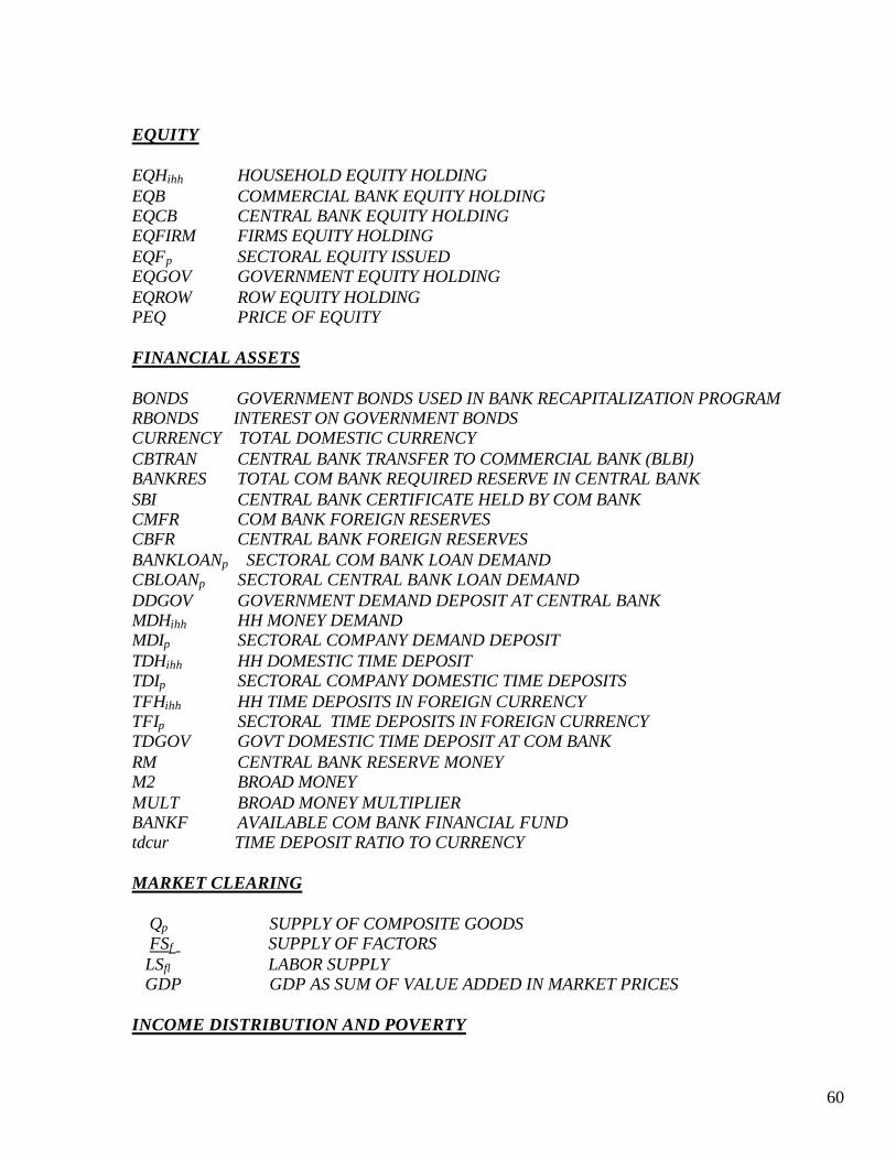
60

EQUITY EQHihh HOUSEHOLD EQUITY HOLDING EQB COMMERCIAL BANK EQUITY HOLDING EQCB CENTRAL BANK EQUITY HOLDING EQFIRM FIRMS EQUITY HOLDING EQFp SECTORAL EQUITY ISSUED EQGOV GOVERNMENT EQUITY HOLDING EQROW ROW EQUITY HOLDING PEQ PRICE OF EQUITY FINANCIAL ASSETS BONDS GOVERNMENT BONDS USED IN BANK RECAPITALIZATION PROGRAM RBONDS INTEREST ON GOVERNMENT BONDS CURRENCY TOTAL DOMESTIC CURRENCY CBTRAN CENTRAL BANK TRANSFER TO COMMERCIAL BANK (BLBI) BANKRES TOTAL COM BANK REQUIRED RESERVE IN CENTRAL BANK SBI CENTRAL BANK CERTIFICATE HELD BY COM BANK CMFR COM BANK FOREIGN RESERVES CBFR CENTRAL BANK FOREIGN RESERVES BANKLOANp SECTORAL COM BANK LOAN DEMAND CBLOANp SECTORAL CENTRAL BANK LOAN DEMAND DDGOV GOVERNMENT DEMAND DEPOSIT AT CENTRAL BANK MDHihh HH MONEY DEMAND MDIp SECTORAL COMPANY DEMAND DEPOSIT TDHihh HH DOMESTIC TIME DEPOSIT TDIp SECTORAL COMPANY DOMESTIC TIME DEPOSITS TFHihh HH TIME DEPOSITS IN FOREIGN CURRENCY TFIp SECTORAL TIME DEPOSITS IN FOREIGN CURRENCY TDGOV GOVT DOMESTIC TIME DEPOSIT AT COM BANK RM CENTRAL BANK RESERVE MONEY M2 BROAD MONEY MULT BROAD MONEY MULTIPLIER BANKF AVAILABLE COM BANK FINANCIAL FUND tdcur TIME DEPOSIT RATIO TO CURRENCY MARKET CLEARING Qp SUPPLY OF COMPOSITE GOODS FSf SUPPLY OF FACTORS LSfl LABOR SUPPLY GDP GDP AS SUM OF VALUE ADDED IN MARKET PRICES INCOME DISTRIBUTION AND POVERTY

61

YHHihh HOUSEHOLD INCOME Y0shh HH INCOME FROM THE ACTUAL SUSENAS SAMPLE (>200 THOUSAND HH) Zu POVERTY LINE IN URBAN AREAS Zr POVERTY LINE IN RURAL AREAS gYihh ENDOGENOUSLY DETERMINED GROWTH OF MEAN HH INCOME Yshh SIMULATED HH INCOME BASED ON BASE-YEAR SUSENAS SAMPLE (MULTIPLIED BY gYihh) Pihh

? ??????????????????FGT POVERTY MEASURE (? RANGES FROM 0 TO 2) C) PARAMETERS dcur DEMAND DEPOSIT RATIO TO CURRENCY mpsihh MARGINAL PROPENSITY TO SAVE BY HOUSEHOLD TYPE transihhihh,ihhh INTER-HOUSEHOLDS TRANSFER RATE ctax TAX RATE FOR CORPORATE INCOME curatihh HOUSEHOLD CURRENCY HOLDING IN DEMAND FOR NARROW MONEY gconsqp SECTORAL SHARES OF GOVERNMENT CONSUMPTION lgrowfl NATURAL GROWTH OF LABOR CATEGORY ?p EXPONENT FOR ARMINGTON FUNCTION ?p EXPONENT FOR CET FUNCTION ? p CES (ARMINGTON) FUNCTION SHARE PARAMETER ? p EXPONENT FOR VALUE ADDED FUNCTION ? p EXPONENT FOR OUTPUT PRODUCTION FUNCTION tmp TARIFF RATES ON IMPORTS tdomp INDIRECT TAX RATES ON DOMESTIC GOODS ttdp TRADE&TRANSPORT MARGIN RATE ON DOMESTIC GOODS ttip TRADE&TRANSPORT MARGIN RATE ON IMPORT GOODS ttindp SHARE OF TTMTOT SPENT ON COMPOSITE GOODS thihh HOUSEHOLD TAX RATE ? p SHIFT PARAMETER FOR PRIVATE INVESTMENT ??p VALUE-ADDED ELASTICITIES FOR PRIVATE INVESTMENT ??p DOMESTIC INTEREST RATE ELASTICITIES FOR PRIVATE INVESTMENT ? 0 INTERCEPT FOR RISK EQUATION ? 1 COEFFICIENT FOR RISK EQUATION degree DEGREE OF OPENESS OF CAPITAL ACCOUNT ? SHARE PARAMETER FOR DOMESTIC AND IMPORTED INTERMEDIATE INPUTS ? 1 COEFFICIENT FOR FOREIGN CAPITAL RELATED TO "degree" ? 0 INTERCEPT FOR FOREIGN CAPITAL (AUTONOMOUS) aadp,pp INPUT-OUTPUT COEFFICIENT FOR DOMESTIC INTERMEDIATE aamp,pp INPUT-OUTPUT COEFFICIENT FOR IMPORTED INTERMEDIATE aaqp,pp INPUT-OUTPUT COEFFICIENT abp INTERMEDIATE INPUT FUNCTION SHIFT PARAMETER acp ARMINGTON FUNCTION SHIFT PARAMETER

62

atp CET FUNCTION SHIFT PARAMETER avp VALUE ADDED FUNCTION SHIFT PARAMETER axp OUPUT PRODUCTION FUNCTION SHIFT PARAMETER bcp ARMINGTON FUNCTION SHARE PARAMETER brow1 SHIFT PARAMETER FOR COMMERCIAL BANK FUND ALLOCATION brow2 EXPONENT FOR COMMERCIAL BANK FUND ALLOCATION alphqp,ihh HHLD CONSUMPTION SHARE PARAMETER (COBB-DOUGLAS) btp CET FUNCTION SHARE PARAMETER ? p,f FACTOR SHARE PARAMETER FOR VALUE ADDED FUNCTION ? p OUTPUT PRODUCTION FUNCTION SHARE PARAMETER wtdp SECTORAL WEIGHTS FOR DOMESTIC PRICE INDEX wtqp SECTORAL WEIGHTS FOR COMPOSITE PRICE INDEX ggconsqp SECTORAL SHARE FOR GOVERNMENT CONSUMPTION GOVINVp SECTORAL GOVERNMENT INVESTMENT GTRANTOT TOTAL GOVT TRANSFERS TO HOUSEHOLDS ROWTRAN ihh FOREIGN TRANSFERS TO HOUSEHOLDS resd RESERVE REQUIREMENT ON DEMAND DEPOSIT rest RESERVE REQUIREMENT ON TIME DEPOSIT rrsec RESERVE REQUIREMENT FOR SECTORAL FOREIGN LOAN rrbank RESERVE REQUIREMENT FOR COMMERCIAL BANK LOAN rrgov RESERVE REQUIREMENT FOR GOVERNMENT LOAN invp RATIO OF INVENTORY INVESTMENT TO GROSS OUTPUT capmatp,pp CAPITAL MATRIX pwep WORLD PRICE OF EXPORTS pwmp WORLD PRICE OF IMPORTS rk CONSUMPTION SHARE OF RURAL HH FOR 4 COMMODITIES (k=1..4) uk CONSUMPTION SHARE OF URBAN HH FOR 4 COMMODITIES (k=1..4) factoini,f COEFFICIENT FOR MAPPING FACTOR INCOME TO INSTITUTIONS POLRISK POLITICAL RISK PORTFOLIO SHARES bb1 SHARE OF SBI IN BANK FUND gh1ihh SHARE OF HH PORTFOLIO IN TIME DEPOSIT gh2ihh SHARE OF HH TIME DEPOSIT IN DOMESTIC TIME DEPOSIT fb2 SHARE OF BANK FUND IN LOAN frow SHARE OF FOREIGN CAPITAL IN PRIVATE BORROWING

63

References

Armington, P. (1969), A Theory of Demand for Products Distinguished by Place of Production, International Monetary Fund Staff Papers, vol.16: 159-178. Aghion, P., Bacchetta, P., and Banerjee, A. (1999), A Simple Model of Monetary Policy and Currency Crises, mimeo. Asher, M. (forthcoming), The Future of Retirement Protection in Southeast Asia, The International Social Security Review, 51. Azis, Iwan J (1997) The Increasing Role of the Urban Non-formal Sector in Indonesia: Employment Analysis within a Multisectoral Framework, in Gavin W. Jones & Pravin Visaria (eds), Urbanization in Large Developing Countries: China, Indonesia, Brazil and India, Clarendon Press, Oxford. _______________ (1998a), Transition from Financial Crisis to Social Crisis, Social Implications of the Asian Financial Crisis, jointly published by UNDP and Korean Development Institute, Seoul.

__________(1998b), When Politics Fuses with Currency Panic, Capital Trend, January, Vol 3, No 2 ___________ (1999), Exchange Rate, Capital Flows and Reform Sequencing in Indonesia: Policy Trend and CGE Model Application, in Julio de Brun and Rolf Lüders (eds), Macroeconomic Policy and the Exchange Rate, International Center for Economic Growth (ICEG), San Francisco __________ (2000a), Simulating Economy-wide Models to Capture the Transition from Financial Crisis to Social Crisis, The Annals of Regional Science, Springer-Verlag, Vol 34:1-28. __________ (2000b) Non-Linear General Equilibrium Impacts of Financial Crisis and Manufacturing Downfall, The Developing Economies, Tokyo-Japan. ___________(2000c) Modeling the Transition From Financial Crisis to Social Crisis, Asian Economic Journal, Vol. 14, No.4, Blackwell. Bernanke, B & Gertler, M. (1989), Agency Costs, Net Worth, and Economic Fluctuations, American Economic Review 79, 14-31. Central Bureau of Statistics (1998), Survey on Crisis Impacts on Cost of Production and Informal Sector. _____________________ , SAKERNAS, various volumes ______________________, SUSENAS, various volumes Dhanani, S and I. Islam (2000), Poverty, Inequality and Social Protection in a Period of Economic Crisis: The Case of Indonesia, unpublished paper for UNSFIR

64

Defourny, J and E. Thorbecke (1984), Structural Path Analysis and Multiplier Decomposition Within A Social Accounting Matrix Framework, Economic Journal, 94, pp.111-136. Decaluwe, B., A. Patry., L. Savard, and E. Throbecke (1999), General Equilibrium Approach for Poverty Analysis, Mimeo, Dept. of Economics, Laval University. Foster, J., J. Greer and E. Thorbecke (1984), A Class of Decomposable Poverty Measures, Econometrica 52. Harberger, A (2000), Monetary Policy in Post-Crisis Period, report for the USAID, February, Jakarta. Irawan, P., and H. Romdiati (1999), The Impacts of Crisis on Poverty and Its Implications for Development Strategies, paper presented at National Workshop on Food and Nutrition VII, Jakarta, May 10-12. Klein, L. (1998), The Asian Economic Crisis, a paper delivered to the Second Committee of the UN General Assembly, October 7. Krugman, P. (1999), Analytical Afterthoughts on the Asian Crisis, mimeo. Leechor, C., (1996), Reforming Indonesia’s Pension System, The World Bank Policy Research Working Paper, No 1677. Manning, C. (2000), Labour Market Adjustment to Indonesia’s Economic Crisis: Context, Trends and Implications, Bulletin of Indonesian Economic Studies, Vol 36, No 1, April. Mishkin, Frederic, S (1998), International Capital Movements, Financial Volatility and Financial Instability, NBER Working Paper, No. 6390, Cambridge, MA Papanek, G. and B.S. Handoko (1999), The Impact on the Poor of Growth and Crisis Evidence from Real Wage Data, paper presented at the conference on “The Economic Issues Facing the New Government,” Jakarta, August. Pradhan, M & R. Sparrow (2000), Indonesia Health Sector Analysis – Changes in health indicators collected in the 1995, 1997, 1998 and 1999 SUSENAS household surveys, mimeo, Cornell University, February 9. Pradhan, M & Sparrow (2000A). Basic Education Outcomes During Crisis: An Analysis Using the 1995, 1997, 1998 and 1999 SUSENAS, mimeo, Cornell University, February 15. Sachs, J.D., A. Tornell., A.Velasco. (1996), Financial Crises in Emerging Markets: The Lessons From 1995, Brookings Papers on Economic Activity, No 1. Sen, A.K. (1999), Development as Freedom, New York: Alfred Knof

65

Srinivasan, T.N. (1994) Data Base for Development Analysis: An Overview, Journal of Development Economics, 44. Suryahadi, A., S. Sumarto., Y. Suharso., Lan Pritchett (2000), The Evolution of Poverty During the Crisis in Indonesia, 1996 to 1999, unpubliseh paper for SMERU. Sutanto, A., P.B. Irawan., A. Said (1999), Poverty Measurement: Problems and Development, paper presented at “International Conference on Methodologies of Poverty Calculation in Indonesia, 1999,” Jakarta, November. Thorbecke, E., et.al., 1992. Adjustment and Equity in Indonesia, Development Center Studies, Paris, OECD. Willem Thorbecke, 2001, “Incorporating Credit Factors into a CGE Model of the Indonesian Economy,” mimeo, George Mason University, February. Tobin, J (1970), A general Equilibrium Approach to Monetary Theory, Journal of Money, Credit and Banking, November, 2, 461-72. World Bank (2000), East Asia Brief: East Asia’s Recovery, Gathering Force, East Asia and Pacific Region, The World Bank, presented in Tokyo, September 18.