Modeling the Modeling the MagnetosphereMagnetosphere

Dr. Ramon LopezDr. Ramon Lopez

The MagnetosphereThe Magnetosphere

When the solar wind When the solar wind encounters a encounters a magnetized body, it is magnetized body, it is slowed and deflectedslowed and deflected

The resulting cavity in The resulting cavity in the solar wind the solar wind controlled by the controlled by the body’s magnetic field body’s magnetic field is called a is called a magnetospheremagnetosphere

Simulations show how this happensSimulations show how this happens

The Earth’s The Earth’s undisturbed field is undisturbed field is basically a dipolebasically a dipole

When the solar wind When the solar wind flows in from the left, flows in from the left, the Earth’s field is the Earth’s field is deformeddeformed

QuickTime™ and aYUV420 codec decompressor

are needed to see this picture.

Magnetospheric “Geography”Magnetospheric “Geography”

Currents flow along the Currents flow along the magnetic fieldmagnetic field

Field Aligned currents light up the Field Aligned currents light up the sky. We call it the Aurorasky. We call it the Aurora

Other planets have aurora too!Other planets have aurora too!

What is the right physics?What is the right physics?

1)1) Electricity and Magnetism - the Electricity and Magnetism - the Maxwell EquationsMaxwell Equations

2)2) Fluid Flow equationsFluid Flow equations3)3) RelativityRelativity4)4) Both 1 and 2Both 1 and 25)5) Both 2 and 3Both 2 and 36)6) 1, 2, and 31, 2, and 3

Given the problem of modeling the flow of the solar wind past the Earth’s magnetic field, what is the proper physics we need to include?

Ideal MHD EquationsIdeal MHD EquationsNon Conservative FormulationNon Conservative Formulation

No strict numerical conservation of energy and momentumNo strict numerical conservation of energy and momentum Various numerical issuesVarious numerical issues

• Errors in propagating strong shocksErrors in propagating strong shocks• Errors in RH ConditionsErrors in RH Conditions• Incorrect shock speedsIncorrect shock speeds

Ideal MHD EquationsIdeal MHD EquationsFull Conservative FormulationFull Conservative Formulation

Strict numerical conservation of mass, momentum Strict numerical conservation of mass, momentum and energyand energy

Numerical difficulties in regions where p<<BNumerical difficulties in regions where p<<B22 negative pressures possible because p becomes negative pressures possible because p becomes difference of two large numbersdifference of two large numbers

Ideal MHD EquationsIdeal MHD EquationsGas Conservative FormulationGas Conservative Formulation

Strict numerical conservation of mass, momentum and plasma Strict numerical conservation of mass, momentum and plasma energyenergy• no strict conservation of total energyno strict conservation of total energy

No difficulties in regions where p<<BNo difficulties in regions where p<<B22

Could use ‘Could use ‘ switch’ to combine with full conservative scheme switch’ to combine with full conservative scheme

Time out to thinkTime out to think

MHD equations can be cast in different MHD equations can be cast in different forms. We chose a particular form to forms. We chose a particular form to solve numerically becausesolve numerically because• 1) they require less computer time1) they require less computer time• 2) they will not allow numerically unphysical 2) they will not allow numerically unphysical

resultsresults• 3) they are easier to solve mathematically3) they are easier to solve mathematically• 4) they are smaller set of equations4) they are smaller set of equations

Computation GridsComputation Grids Simulation boundaries should be in Simulation boundaries should be in

supermagnetosonic flow regimessupermagnetosonic flow regimes• 18 Re from Earth on Sunward side18 Re from Earth on Sunward side• 200 Re in tailward direction200 Re in tailward direction• 50 Re in transverse directions50 Re in transverse directions

A variety of grid types exist with varying A variety of grid types exist with varying degrees of complexitydegrees of complexity

• Uniformed CartesianUniformed Cartesian• Stretched CartesianStretched Cartesian• Nested Cartesian Nested Cartesian • Regular NoncartesianRegular Noncartesian• Irregular NoncartesianIrregular Noncartesian

Stretched Cartesian GridStretched Cartesian Grid• Low programming overheadLow programming overhead• Low computing overheadLow computing overhead• No memory overheadNo memory overhead• Easy parallelizationEasy parallelization• Somewhat adaptableSomewhat adaptable

Example from Raeder UCLA Example from Raeder UCLA MHD ModelMHD Model

Uniformed Cartiesian GridUniformed Cartiesian Grid• Low programming overheadLow programming overhead• Low computing overheadLow computing overhead• No memory overheadNo memory overhead• Easy parallelizationEasy parallelization• Not very adaptableNot very adaptable

Regular NoncartesianRegular Noncartesian• Medium programming Medium programming

overheadoverhead

• Low memory overheadLow memory overhead

• small computing overheadsmall computing overhead

• parallelizes like regular parallelizes like regular cartesian gridcartesian grid

• somewhat adaptablesomewhat adaptable Example from LFMExample from LFM

Nested CartesianNested Cartesian• Medium/High programming Medium/High programming

overheadoverhead• Medium/High memory overheadMedium/High memory overhead• small computational overheadsmall computational overhead• difficult to parallelizedifficult to parallelize• very (self) adaptablevery (self) adaptable

Example from BATS-R-USExample from BATS-R-US

Boundary ConditionsBoundary Conditions Upstream Upstream

• Fixed or time dependent values for 8 plasma Fixed or time dependent values for 8 plasma parametersparameters

Can be idealized for derived from solar wind Can be idealized for derived from solar wind observationsobservations

• Problem with BProblem with BXX Need to know 3D structure of solar wind becauseNeed to know 3D structure of solar wind because

Implies BImplies BXX=B=BNN cannot change if solar parameters are cannot change if solar parameters are independent of Y and Zindependent of Y and Z

Find Find n n direction with no variation and then sweep these direction with no variation and then sweep these fronts across front boundaryfronts across front boundary

0()0upstreamdownstreamBB∇•=⇔•−=Bn

Boundary Conditions IIBoundary Conditions II All other sidesAll other sides

• Free flow conditions for plasma and transverse Free flow conditions for plasma and transverse components of components of BB

• normal component of normal component of BB flows from flows from BB=0=0 Inner Boundary ConditionInner Boundary Condition

• MI Coupling moduleMI Coupling module• Hard wall boundary condition for normal Hard wall boundary condition for normal

component of velocity and densitycomponent of velocity and density

0∂Ψ=∂n

Magnetosphere-Ionosphere Magnetosphere-Ionosphere Coupling Coupling

Inner boundary of MHD domain is placed between 2-4 RInner boundary of MHD domain is placed between 2-4 REE

from the Earthfrom the Earth• High Alfven speeds in this region would impose strong limitations on global High Alfven speeds in this region would impose strong limitations on global

step sizestep size• Physical reasonable since MHD not the correct description of the physics Physical reasonable since MHD not the correct description of the physics

occuring within this regionoccuring within this region• Covers the high latitude region of the ionosphere (45Covers the high latitude region of the ionosphere (45-90-90))

Parameters in MHD region are mapped along static dipole field lines Parameters in MHD region are mapped along static dipole field lines into the ionosphereinto the ionosphere

Field aligned currents (FACs) and precipitation parameters are used to Field aligned currents (FACs) and precipitation parameters are used to solve for ionospheric potential which is mapped back to inner boundary solve for ionospheric potential which is mapped back to inner boundary as boundary condition for flowas boundary condition for flow

2()B−∇Φ×=Bv

Ionosphere ModelIonosphere Model

• 2D Electrostatic Model

P

HΦ=J||

Φ=0 at low latitude boundary of ionosphere

• Conductivity Models– Solar EUV ionization

• Creates day/night and winter/summer asymmetries

– Auroral Precipitation • Empirical determination of energetic electron precipitation

2/32/3o10.71/2o10.70.5(cos) 651.8cos 65pHFFχχχχ=∀≤=∀≤

Auroral Precipitation ModelAuroral Precipitation Model Emperical relationships are used to convert MHD parameters Emperical relationships are used to convert MHD parameters

into a characteristic energy and flux of the precipitating into a characteristic energy and flux of the precipitating electronselectrons• Initial flux and energyInitial flux and energy

• Parallel Potential drops (Knight relationship)Parallel Potential drops (Knight relationship)

• Effects of geomagnetic fieldEffects of geomagnetic field

• Hall and Pederson Conductance from electron precp (Hardy)Hall and Pederson Conductance from electron precp (Hardy)

21/2o osocεαφρε==

1/2oRJεερ=PP

787 0 0ooooeeεεεεφφεφφε−⎛⎞⎜⎟=−∀>⎜⎟⎝⎠=∀<PPPP

oεεε=P

3/21/20.85H25 0.4510.0625ppεφεεΣ=Σ=Σ+

Time Out to ThinkTime Out to Think

LFM contains how many separate LFM contains how many separate ‘computational’ models and ‘physical’ ‘computational’ models and ‘physical’ domainsdomains• 1) 2 models and 1 domain1) 2 models and 1 domain• 2) 3 models and 2 domains2) 3 models and 2 domains• 3) 1 model and 2 domain3) 1 model and 2 domain• 4) 2 models and 2 domains4) 2 models and 2 domains

MHD Magnetosphere SimulationMHD Magnetosphere Simulation The Lyon-Fedder-Mobary (LFM) code is a The Lyon-Fedder-Mobary (LFM) code is a

fully 3-D MHD simulation run with real solar fully 3-D MHD simulation run with real solar wind inputwind input

Magnetosphere modeled via ideal MHD Magnetosphere modeled via ideal MHD equations within 30 to equations within 30 to 300R300REE (x) and 100 R(x) and 100 REE (y,z)(y,z) Upstream and side BCs -> Solar wind dataUpstream and side BCs -> Solar wind data Downstream BC -> Supersonic outflowDownstream BC -> Supersonic outflow Inner BC -> 2-D Ionospheric simulationInner BC -> 2-D Ionospheric simulation

Reconnection occurs due to numerical effectsReconnection occurs due to numerical effects

Visualizing the resultsVisualizing the results In order to understand a a global sense what In order to understand a a global sense what

the simulation produced, you have to visualize the simulation produced, you have to visualize the resultsthe results

We use package called OpenDX, which is an We use package called OpenDX, which is an open-source version of IBM DataExploreropen-source version of IBM DataExplorer

Another package, SPDX, provides modules Another package, SPDX, provides modules for reading the simulation HDF filesfor reading the simulation HDF files

Images are rendered frame by fame, then Images are rendered frame by fame, then strung together as moviesstrung together as movies

QuickTime™ and aYUV420 codec decompressor

are needed to see this picture.

QuickTime™ and aVideo decompressor

are needed to see this picture.

QuickTime™ and aYUV420 codec decompressor

are needed to see this picture.

QuickTime™ and aVideo decompressor

are needed to see this picture.

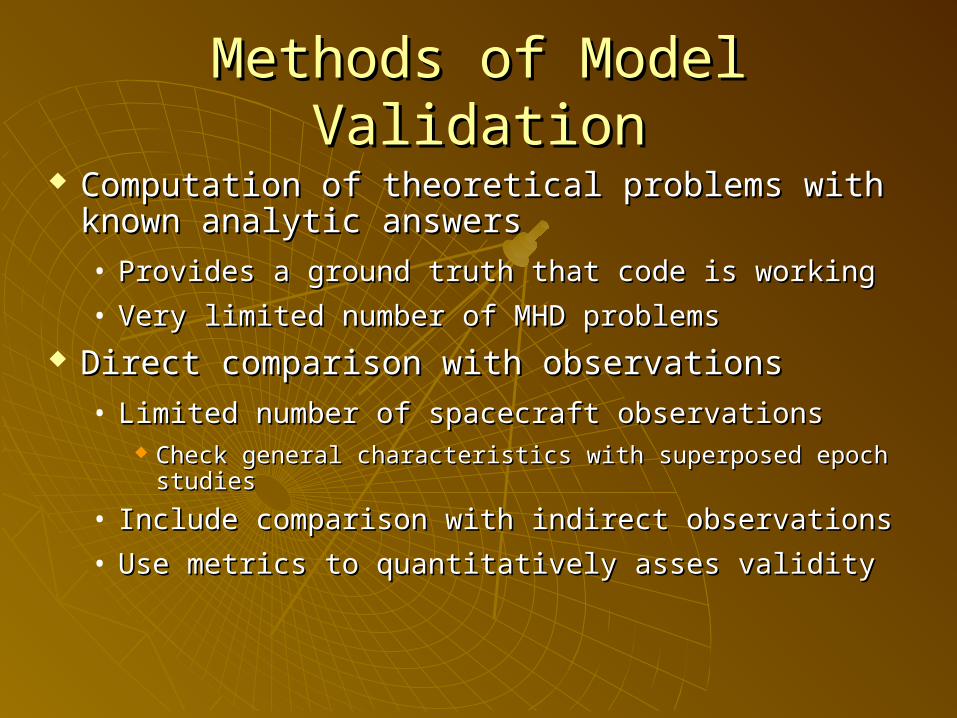
Methods of Model ValidationMethods of Model Validation

Computation of theoretical problems with known Computation of theoretical problems with known analytic answersanalytic answers

• Provides a ground truth that code is workingProvides a ground truth that code is working

• Very limited number of MHD problems Very limited number of MHD problems

Direct comparison with observationsDirect comparison with observations

• Limited number of spacecraft observationsLimited number of spacecraft observations Check general characteristics with superposed epoch studiesCheck general characteristics with superposed epoch studies

• Include comparison with indirect observations Include comparison with indirect observations

• Use metrics to quantitatively asses validityUse metrics to quantitatively asses validity

The March 9, 1995 SubstormThe March 9, 1995 Substorm Clean, isolated, Clean, isolated,

multiple onset multiple onset substormsubstorm

Simulated AL and Simulated AL and CANOPUS AL CANOPUS AL agree quite wellagree quite well

Other simulated Other simulated features agree features agree well with the well with the observationsobservations

LFM simulation results are similar LFM simulation results are similar to AIME resultsto AIME results

Where does the energy come Where does the energy come from?from?

Magnetic Magnetic reconnection is the reconnection is the process by which process by which magnetic energy is magnetic energy is converted into plasma converted into plasma energyenergy

Reconnection plays a Reconnection plays a basic role in the basic role in the dynamics of space dynamics of space plasmasplasmas

IMF coupling to the magnetosphereIMF coupling to the magnetosphere Magnetic merging on Magnetic merging on

the dayside between the dayside between the northward the northward geomagnetic field (1) geomagnetic field (1) and southward IMF (2) and southward IMF (2) allows solar wind allows solar wind energy to enter the energy to enter the magnetosphere (3,4)magnetosphere (3,4)

Reconnection on the Reconnection on the nightside (6) releases nightside (6) releases energy stored as energy stored as magnetic flux in the tail magnetic flux in the tail lobes (5)lobes (5)