Modeling the effects of dynamic range compressionon signals in noise

Ryan M. Coreya) and Andrew C. Singerb)

Electrical and Computer Engineering, University of Illinois Urbana-Champaign, Urbana, Illinois 61801, USA

ABSTRACT:Hearing aids use dynamic range compression (DRC), a form of automatic gain control, to make quiet sounds louder

and loud sounds quieter. Compression can improve listening comfort, but it can also cause unwanted distortion in

noisy environments. It has been widely reported that DRC performs poorly in noise, but there has been little

mathematical analysis of these noise-induced distortion effects. This work introduces a mathematical model to study

the behavior of DRC in noise. By making simplifying assumptions about the signal envelopes, we define an effective

compression function that models the compression applied to one signal in the presence of another. Using the proper-

ties of concave functions, we prove results about DRC that have been previously observed experimentally: that the

effective compression applied to each sound in a mixture is weaker than it would have been for the signal alone; that

uncorrelated signal envelopes become negatively correlated when compressed as a mixture; and that compression

can reduce the long-term signal-to-noise ratio in certain conditions. These theoretical results are supported by soft-

ware experiments using recorded speech signals. VC 2021 Acoustical Society of America.

https://doi.org/10.1121/10.0005314

(Received 20 November 2020; revised 27 May 2021; accepted 29 May 2021; published online 9 July 2021)

[Editor: Hari M. Bharadwaj] Pages: 159–170

I. INTRODUCTION

Hearing aids often perform poorly in noisy environ-

ments, where people with hearing loss need help most. One

challenge for hearing aids in noise is a nonlinear processing

technique known as dynamic range compression (DRC),

which improves audibility and comfort by making quiet

sounds louder and loud sounds quieter (Allen, 2003; Kates,

2005; Souza, 2002; Villchur, 1973). Compression is used in

all modern hearing aids, but it can cause unwanted distortion

when applied to multiple overlapping sounds. For example, a

sudden noise can reduce the gain applied to speech sounds.

This effect is well documented empirically but has been little

studied mathematically. To better understand DRC in noisy

environments, this work applies tools from signal processing

theory to model the effects of DRC on sound mixtures.

The auditory systems of people with hearing loss often

have reduced dynamic range: Quiet sounds need to be

amplified in order to be audible, but loud sounds can cause

discomfort. Hearing aids with DRC apply level-dependent

amplification so that the output signal has a smaller dynamic

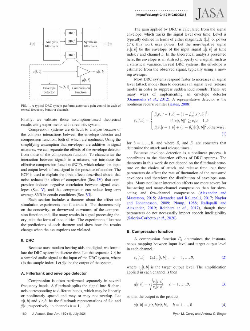
range than the input signal. A typical DRC system is shown

in Fig. 1. An envelope detector tracks the level of the input

signal over time in one or more frequency bands while a

compression function adjusts the amplification to keep the

output level within a comfortable range. Both the envelope

detector and the compression function are nonlinear pro-

cesses, so when the input contains sounds from multiple

sources, changes in one component signal can affect the

processing applied to the others.

This interaction between signals can be difficult to mea-

sure, but hearing researchers have found three quantifiable

effects. First, noise can reduce the effect of a compressor,

especially at low signal-to-noise ratios (SNR) (Souza et al.,2006). The DRC system applies gain based on the stronger

signal and has little effect on the dynamic range of the

weaker signal. This effect can measured by comparing the

overall dynamic ranges of the input and output signals

(Braida et al., 1982; Stone and Moore, 1992). Second, fluc-

tuations in the input level of one component signal vary the

output levels of other components. This interaction has been

called across-source modulation (Stone and Moore, 2007)

and can be measured using the correlation coefficient

between output envelopes. Finally, at high SNR, compres-

sors tend to amplify low-level noise more strongly than the

higher-level signal of interest, which can reduce the long-

term average SNR (Alexander and Masterson, 2015;

Hagerman and Olofsson, 2004; Rhebergen et al., 2009;

Souza et al., 2006).

The adverse effects of noise on DRC systems have been

well documented empirically, but the problem has received

little formal mathematical analysis. While experimental

work is useful for studying the consequences of these effects,

especially on human listeners, theoretical results can help to

understand their causes. This work applies signal processing

research methods to the DRC distortion problem: First, we

make simplifying assumptions to develop a tractable mathe-

matical model of a complex system. Next, we use that model

to prove theorems that explain the behavior of the system.

a)Electronic mail: corey1@illinois.edu, ORCID: 0000-0002-3122-124X.b)ORCID: 0000-0001-9926-7036.

J. Acoust. Soc. Am. 150 (1), July 2021 VC 2021 Acoustical Society of America 1590001-4966/2021/150(1)/159/12/$30.00

ARTICLE...................................

Finally, we validate those assumption-based theoretical

results using experiments with a realistic system.

Compression systems are difficult to analyze because of

the complex interactions between the envelope detector and

compression function, both of which are nonlinear. Using the

simplifying assumption that envelopes are additive in signal

mixtures, we can separate the effects of the envelope detector

from those of the compression function. To characterize the

interaction between signals in a mixture, we introduce the

effective compression function (ECF), which relates the input

and output levels of one signal in the presence of another. The

ECF is used to explain the three effects described above: that

noise reduces the effect of compression (Sec. IV), that com-

pression induces negative correlation between signal enve-

lopes (Sec. V), and that compression can reduce long-term

average SNR in certain conditions (Sec. VI).

Each section includes a theorem about the effect and

simulation experiments that illustrate it. The theorems rely

on the concavity, or downward curvature, of the compres-

sion function and, like many results in signal processing the-

ory, take the form of inequalities. The experiments illustrate

the predictions of each theorem and show how the results

change when the assumptions are violated.

II. DRC

Because most modern hearing aids are digital, we formu-

late the DRC system in discrete time. Let the sequence ~x½t� be

a sampled audio signal at the input of the DRC system, where

t is the sample index. Let ~y½t� be the output of the system.

A. Filterbank and envelope detector

Compression is often performed separately in several

frequency bands. A filterbank splits the signal into B chan-

nels corresponding to different bands, which may be linearly

or nonlinearly spaced and may or may not overlap. Let

x½t; b� and y½t; b� be the filterbank representations of ~x½t� and

~y½t�, respectively, in channels b ¼ 1;…;B.

The gain applied by DRC is calculated from the signal

envelope, which tracks the signal level over time. Level is

typically defined in terms of either magnitude (jxj) or power

(x2); this work uses power. Let the non-negative signal

vx½t; b� be the envelope of the input signal x½t; b� at time

index t and channel b. In the theoretical analysis presented

here, the envelope is an abstract property of a signal, such as

a statistical variance. In real DRC systems, the envelope is

estimated from the observed signal, typically using a mov-

ing average.

Most DRC systems respond faster to increases in signal

level (attack mode) than to decreases in signal level (release

mode) in order to suppress sudden loud sounds. There are

many ways of implementing an envelope detector

(Giannoulis et al., 2012). A representative detector is the

nonlinear recursive filter (Kates, 2008),

vx t; b½ � ¼bavx t� 1; b½ � þ ð1� baÞjx t; b½ �j2;

if jx t; b½ �j2 � vx t� 1; b½ �brvx t� 1; b½ � þ ð1� brÞjx t; b½ �j2; otherwise;

8>><>>:

(1)

for b ¼ 1;…;B; and where ba and br are constants that

determine the attack and release times.

Because envelope detection is a nonlinear process, it

contributes to the distortion effects of DRC systems. The

theorems in this work do not depend on the filterbank struc-

ture or the choice of attack and release time, but these

parameters do affect the rate of fluctuation of the measured

envelopes and therefore the distribution of envelope sam-

ples. Many nonlinear interaction effects are more severe for

fast-acting and many-channel compression than for slow-

acting and few-channel compression (Alexander and

Masterson, 2015; Alexander and Rallapalli, 2017; Naylor

and Johannesson, 2009; Plomp, 1988; Rallapalli and

Alexander, 2019; Reinhart et al., 2017), though these

parameters do not necessarily impact speech intelligibility

(Salorio-Corbetto et al., 2020).

B. Compression function

A compression function Cb determines the instanta-

neous mapping between input level and target output level

in each channel,

vy t; b½ � ¼ Cb vx t; b½ �ð Þ; b ¼ 1;…;B; (2)

where vy½t; b� is the target output level. The amplification

applied in each channel is then

g t; b½ � ¼

ffiffiffiffiffiffiffiffiffiffiffiffiffivy t; b½ �vx t; b½ �

s; b ¼ 1;…;B; (3)

so that the output is the product

y t; b½ � ¼ g t; b½ �x t; b½ �; b ¼ 1;…;B: (4)

FIG. 1. A typical DRC system performs automatic gain control in each of

several frequency bands or channels.

160 J. Acoust. Soc. Am. 150 (1), July 2021 Ryan M. Corey and Andrew C. Singer

https://doi.org/10.1121/10.0005314

Note that the target output level vy½t; b� is not necessar-

ily equal to the measured envelope of y½t; b� because the

envelope is a moving average. Longer release times cause

gains to lag behind short-term signal levels, especially for

dynamic signals such as speech (Braida et al., 1982; Stone

and Moore, 1992).

Although compression functions are defined here in

terms of input and output level (i.e., power), they are often

visualized and described on a logarithmic scale, such as in

decibels (dB). A typical “knee-shaped” compression func-

tion is shown in Fig. 2: It features a linear region in which

gain is constant, a compressive region where the output

level increases by less than the input level, and and a limit-

ing region that prevents the output from exceeding a maxi-

mum safe level.

The strength of compression can be characterized by

the compression ratio (CR), which is the inverse of the slope

of the compression function on a log-log scale, as shown in

Fig. 2. For example, in a 3:1 compressor, the output

increases by 1 dB for every 3 dB increase in the input. For a

constant CR, the compression function is given by the

power-law relationship

CbðvÞ ¼ G0 b½ �vð1=CRÞ; (5)

where G0½b� is a constant power gain factor. Thus, for a 3:1

compressor, the output level is proportional the cube root of

the input level. In limiters, CbðvÞ is constant and so the CR

is infinite.

While most compressors reported in the literature use

some combination of linear, power-law, and limiting com-

pression functions, many others are possible. To make our

analysis as general as possible, we allow the compression

function to be any mapping between non-negative numbers

such that the output level grows no faster than the input

level. More precisely, we require it to be a concave

function.

Definition 1. A function CbðvÞ is a compression functionif it is concave, non-negative, and nondecreasing for all v > 0.

In mathematics, a function f(x) is said to be concave if

for any k 2 ½0; 1� and any x1 and x2,

f ðkx1 þ ð1� kÞx2Þ � kf ðx1Þ þ ð1� kÞf ðx2Þ: (6)

Note that Definition 1 includes non-differentiable functions

such as knee-shaped compression curves. It excludes

dynamic range expanders, which some hearing aids apply at

low signal levels to reduce noise. The proofs in this work

will also involve convex functions that satisfy Eq. (6) with

the inequality reversed. Convex and concave functions are

widely used to prove inequalities in signal processing and

information theory (Cover and Thomas, 2006).

To describe how much a compression function reduces

the dynamic range of a signal, we could compute its CR.

Because the CR can be infinite, however, it is more conve-

nient to work with its inverse, the compression slope.

Definition 2. For all points v at which a compression

function CbðvÞ is differentiable, the compression slopeCSbðvÞ is the slope of CbðvÞ on a log-log scale,

CSbðvÞ ¼d

duln Cb euð Þju¼ln v; (7)

¼ C0bðvÞCbðvÞ

v: (8)

For example, if CbðvÞ ¼ G0½b�va, then CSbðvÞ ¼ a for

all v. The smaller the compression slope, the more the

dynamic range of the signal is reduced.

C. Experimental methods

To validate the predictions of the mathematical model,

each section of this work includes experiments using speech

recordings and a software DRC system. The theoretical

results in this work rely on simplifying assumptions, but the

simulation experiments are more realistic and therefore

illustrate the limitations of the model. Wherever possible,

the experiments use methods and performance metrics from

prior work in the literature.

Although the compression function varies with each

experiment, all simulations in this work use the same envelope

detector. The input is first processed by a short-time Fourier

transform with 8 ms windows and 50% overlap. A frequency-

domain filterbank splits the signals into 6 Mel-spaced bands

from 0 to 8 kHz, which are roughly linearly spaced at lower

frequencies and exponentially spaced at higher frequencies.

Within each band, the envelopes are computed using the non-

linear recursive filter (1) with an attack time of 10 ms and a

release time of 50 ms as defined by ANSI S3.22–1996 (ANSI,

1996). All speech signals are 60-s clips derived from the

Voice Cloning Toolkit (VCTK) dataset of quasi-anechoic read

speech (Veaux et al., 2017). The figures in this work use loga-

rithmic scales for envelope level. These levels are given in dB

relative to the mean wideband signal level. That is, each

speech signal has a mean level of 0 dB across channels.

III. MODELING COMPRESSION OF SOUND MIXTURES

Hearing aids are often used in noisy environments with

several simultaneous sound sources. The interactions

between multiple signals are difficult to analyze because

DRC involves two nonlinear operations: envelope detection

FIG. 2. A compression function Cb, shown here on a logarithmic scale,

maps input levels to output levels.

J. Acoust. Soc. Am. 150 (1), July 2021 Ryan M. Corey and Andrew C. Singer 161

https://doi.org/10.1121/10.0005314

and level-dependent amplification. To create a tractable

model for sound mixtures, we make a simplifying assump-

tion about the signal envelopes that allows us to separate the

effects of these two nonlinearities, as shown in Fig. 3. Under

this model, the filterbank and envelope detector determine

the relationship between input signals and envelope values;

they act independently on each component signal.

Meanwhile, the compression function determines the output

levels from these envelopes; it acts independently at each

time index and within each channel. In this work, we focus

on the compression function.

A. Envelope model

Suppose that the input to the system is ~x½t� ¼ ~s1½t�þ ~s2½t�, where ~s1½t� and ~s2½t� are two discrete-time signals.

For example, ~s1 and ~s2 could be two speech signals as cap-

tured at the listening device microphone, including any

reverberation effects. Because a filterbank is a linear system,

the filterbank representation of the input is

x t; b½ � ¼ s1 t; b½ � þ s2 t; b½ �; b ¼ 1;…;B; (9)

where s1½t; b� and s2½t; b� are the filterbank representations of

~s1½t� and ~s2½t�, respectively.

Because envelope detection is a nonlinear process, the

additivity property of Eq. (9) does not hold in general for

the signal envelopes measured by practical envelope detec-

tors. However, to simplify our analysis, the signal envelopes

can be modeled as obeying additivity.

Assumption 1. The envelopes vs1½t; b�; vs2

½t; b�, andvx½t; b� of s1½t; b�; s2½t; b�, and x½t; b�, respectively, satisfy

vx t; b½ � ¼ vs1t; b½ � þ vs2

t; b½ �; b ¼ 1;…;B: (10)

This assumption is justified if we think of the envelopes

as abstract properties of signals, such as parameters of a pro-

cess that generates them, rather than as measurements. For

example, suppose that s1½t; b� and s2½t; b� are sample func-

tions of random processes that are uncorrelated with each

other (Hajek, 2015). Then the variance of the mixture is

given by Varðx½t; b�Þ ¼ Varðs1½t; b�Þ þ Varðs2½t; b�Þ. If

vx½t; b� were any linear transformation of the sequence

Varðx½t; b�Þ, then the envelopes would satisfy Assumption 1.

Because the variance is an ensemble average, not a time

average, the processes need not be stationary or ergodic.

Of course, real compression systems cannot observe

the underlying variance of a random process; they derive

envelopes from recorded samples. The accuracy of the

additive envelope model depends on the signals: Two sinus-

oids would strongly violate the assumption (Ludvigsen,

1993), while two signals that are disjoint across time and

channels would satisfy it exactly. To test the accuracy of

the assumption for a realistic envelope detector, we applied

the software envelope detector described in Sec. II C to a

mixture of two speech signals and compared the envelope

of the mixture, vx½t; b�, to the sum of the envelopes of the

component signals, vs1½t; b� þ vs2

½t; b�. Figure 4 shows a set

of envelope samples drawn from different time frames and

frequency channels plotted on a decibel scale. In this exper-

iment, the assumption is accurate to within 1 dB for 93% of

samples.

B. Output model

Care is also required in analyzing the components of

the output of a nonlinear system. Let ~y½t� ¼ ~r1½t� þ ~r2½t�,where ~r1½t� is the component of the output corresponding to

~s1½t� and ~r2½t� is the component corresponding to ~s2½t�. For

systems with the additivity property, like linear filters, these

components can be calculated by applying the same system

to ~s1 and ~s2. For nonlinear systems like DRC, each compo-

nent of the output depends on all components of the input.

In general, nonlinear distortion artifacts cannot be clearly

attributed to one input signal or the other, and they cannot

be easily classified as helpful or harmful to intelligibility

(Ludvigsen, 1993). For the relatively mild compression used

in hearing aids—compared to aggressive compression-based

effects in electronic music, for example—a reasonable

approach is to treat the nonlinear system as a time-varying

linear system.

In this work, the output components are determined by

calculating the level-dependent amplification sequence

FIG. 3. A simplified model separates the effects of the filterbank and enve-

lope detector from those of the compression functions C1;…; CB. The for-

mer act independently across signals, while the latter act independently

across time and channels.

FIG. 4. Empirical evaluation of Assumption 1 with a mixture of two speech

signals. The plotted points are samples of the sum of the envelopes,

vs1½t; b� þ vs2

½t; b�, and the envelope of the sum, vx½t; b�. The inset plot shows

a histogram of the difference 10 log10ðvs1þ vs2

Þ � 10 log10vx.

162 J. Acoust. Soc. Am. 150 (1), July 2021 Ryan M. Corey and Andrew C. Singer

https://doi.org/10.1121/10.0005314

g½t; b� based on the mixture x½t; b�, then applying it to each

component,

y t; b½ � ¼ g t; b½ �x t; b½ � (11)

¼ g t; b½ � s1 t; b½ � þ s2 t; b½ �ð Þ (12)

¼ g t; b½ �s1 t; b½ �|fflfflfflfflfflfflfflffl{zfflfflfflfflfflfflfflffl}r1 t;b½ �

þ g t; b½ �s2 t; b½ �|fflfflfflfflfflfflfflffl{zfflfflfflfflfflfflfflffl}r2 t;b½ �

; (13)

for all time indices t and channels b ¼ 1;…;B. This definition

of the output components is used in the mathematical analysis

below. Similarly, in the software simulations, the two input

signals are stored in memory alongside their mixture and the

amplification sequence is applied separately to each, allowing

the output components to be computed exactly. This time-

varying linear approach to computing output coefficients is

conceptually related to the phase inversion technique of

Hagerman and Olofsson (2004), which is often used in labora-

tory experiments with real hearing aids where the time-

varying amplification sequence cannot be observed directly.

C. Effective compression function

The additive models for the input envelopes and output

signal components, while imperfect, allow us to study the

dominant source of nonlinearity in a DRC system: the com-

pression function. Although the signals s1½t; b� and s2½t; b�may have different levels, the amplification g½t; b� applied to

both of them is the same and is computed from the overall

level of the input signal,

g t; b½ � ¼

ffiffiffiffiffiffiffiffiffiffiffiffiffiffiffiffiffiffiffiffiffiCbðvx t; b½ �Þ

vx t; b½ �

s: (14)

Under Assumption 1, the amplification is

g t; b½ � ¼ffiffiffiffiffiffiffiffiffiffiffiffiffiffiffiffiffiffiffiffiffiffiffiffiffiffiffiffiffiffiffiffiffiffiffiffiffiffiffiffiffiffiCbðvs1

t; b½ � þ vs2t; b½ �Þ

vs1t; b½ � þ vs2

t; b½ �

s; (15)

resulting in the output levels

vr1t; b½ � ¼ Cbðvs1

t; b½ � þ vs2t; b½ �Þ

vs1t; b½ � þ vs2

t; b½ � vs1t; b½ �; (16)

vr2t; b½ � ¼ Cbðvs1

t; b½ � þ vs2t; b½ �Þ

vs1t; b½ � þ vs2

t; b½ � vs2t; b½ �; (17)

for channels b ¼ 1;…;B. The gain and therefore the output

levels are functions of both input signal levels, as illustrated

in Fig. 5. The gain applied to s1½t; b� in the presence of

s2½t; b� is weaker than it would have been for s1½t; b� alone.

To characterize this effect, we can define an effective com-

pression function (ECF) that relates the input and output lev-

els of one signal in the presence of another.

Definition 3. The ECF Cbðv1jv2Þ applied to a signal

with level v1 > 0 in the presence of a signal with level

v2 � 0 is given by

Cbðv1jv2Þ ¼Cbðv1 þ v2Þ

v1 þ v2

v1; (18)

where CbðvÞ is the compression function applied to the mix-

ture level v1 þ v2.

Using this definition, Eqs. (16) and (17) become

vr1t; b½ � ¼ Cbðvs1

t; b½ �jvs2t; b½ �Þ; (19)

vr2t; b½ � ¼ Cbðvs2

t; b½ �jvs1t; b½ �Þ; (20)

for b ¼ 1;…;B. The ECF expresses the dependence

between the levels of the two signal components. The ECF

can be used to mathematically characterize the nonlinear

interactions between signals in DRC systems, including the

effective CR, the across-source modulation effect, and the

SNR.

IV. EFFECTIVE COMPRESSION PERFORMANCE

When DRC is applied to a mixture of multiple signals,

it has a weaker effect on the dynamic range of each compo-

nent signal than it would if they were processed indepen-

dently. Intuitively, if a signal of interest is weaker than a

noise source, then the noise level will determine the gain

applied to both signals and the target signal will not be com-

pressed. Even when the target signal has a higher level, the

noise will cause the gain to decrease less than it should with

respect to the target level.

To quantify the effect of noise on compression perfor-

mance, we can measure the change in the output level of the

target signal in response to a change in its input level and

compare that relationship to the nominal CR. Even without

noise, the long-term effective compression ratio (ECR) is

generally lower than the nominal ratio because of the time-

averaging effects of the envelope detector (Braida et al.,1982; Stone and Moore, 1992). However, it has been

FIG. 5. Gain applied to a mixture signal as a function of the signal enve-

lopes vs1½t; b� and vs2

½t; b� for CbðvÞ ¼ v1=3 under Assumption 1. The length

of the arrows is proportional to the power gain g2½t; b� in dB and the dashed

curve shows the equilibrium mixture level Cbðvs1þ vs2

Þ ¼ vs1þ vs2

.

J. Acoust. Soc. Am. 150 (1), July 2021 Ryan M. Corey and Andrew C. Singer 163

https://doi.org/10.1121/10.0005314

observed that the ECR of a DRC system is further reduced

in the presence of noise (Souza et al., 2006). While this

noise-induced reduction in CR has been previously mea-

sured as a long-term average for particular signals, here we

show that it is a short-term effect caused by the concavity of

the compression function. Although the magnitude of the

reduction depends on the compression function and the sig-

nal characteristics, the effect occurs for every compression

function and at every SNR.

Because the instantaneous CR can be infinite, we will

instead use the effective compression slope, defined as the

log-log slope of the ECF.

Definition 4. If Cbðv1jv2Þ is differentiable with respect to

v1, then the effective compression slope CSbðv1jv2Þ is given by

CSbðv1jv2Þ ¼@

@uCbðeujv2Þju¼ln v1

(21)

¼

@

@v1

Cbðv1jv2Þ

Cbðv1jv2Þv1: (22)

Note that the effective compression slope defined here is

a function of the two signal levels, so it provides a more

complete description of the compression system than the

long-term ECR. Furthermore, it only measures the instanta-

neous effects of interaction between signals, not the time-

averaging effects of the envelope detector. The simplified

envelope model allows us to analyze these two compression-

weakening mechanisms separately.

A. Noise reduces compression performance

Using the properties of the ECF, it can be shown that

the effective compression slope from Definition 4 is always

larger than the nominal compression slope from Definition

2—equivalently, the instantaneous ECR is always smaller

than the nominal CR—meaning that, when applied to a mix-

ture, the system is less compressive on each component sig-

nal than it would be if applied to the components separately,

CSbðvs1jvs2Þ � CSbðvs1

þ vs2Þ; b ¼ 1;…;B: (23)

Notably, this result applies to any pair of signal levels vs1

and vs2. Whereas the across-source modulation result of Sec.

V relies on probabilistic averaging and the SNR result of

Sec. VI uses time averaging, Eq. (23) holds for each individ-

ual envelope sample.

The proof relies on concavity. Because the lemmas and

theorems in this work follow from the properties of com-

pression functions, which act independently across time and

frequency, the time and channel indices ½t; b� are omitted in

their statements and proofs.

Theorem 1. If a compression function CðvÞ is differentia-ble at vx ¼ v1 þ v2, then its effective compression slope satisfies

CSðv1jv2Þ � CSðvxÞ; (24)

with equality if CðvÞ is linear or if v2 ¼ 0.

Proof. Because CðvÞ is defined to be concave and non-

negative for v> 0, it follows that

CðvÞ � vC0ðvÞ � 0 (25)

for all v at which C is differentiable, with equality if C is lin-

ear. The effective compression slope is given by

CSðv1jv2Þ ¼

@

@v1

Cðv1jv2Þ

Cðv1jv2Þv1 (26)

¼ vx

CðvxÞC0ðvxÞv1 þ CðvxÞ

vx� CðvxÞv1

v2x

!(27)

¼ C0ðvxÞCðvxÞ

v1 þ 1� v1

vx(28)

¼ C0ðvxÞCðvxÞ

vx �C0ðvxÞCðvxÞ

v2 þv2

vx(29)

¼ CSðvxÞ þv2

vxCðvxÞðCðvxÞ � vxC0ðvxÞÞ (30)

� CSðvxÞ; (31)

with equality if C is linear or if v2 ¼ 0. �

Suppose that v1 corresponds to a sound source of inter-

est and v2 is the level of unwanted noise. The proof illus-

trates that the effective compression slope for the target

increases with the level of the interfering signal. For exam-

ple, in the limit as v1=vx approaches 0, the slope from Eq.

(28) approaches 1, so that the system applies linear gain to

the target signal. At low SNR, the gain applied to both sig-

nals is determined by the noise. The theorem shows, how-

ever, that even at high SNR, the compression effect is

slightly weaker.

B. Experiments

Theorem 1 shows that under the simplified envelope

model, noise always reduces the effect of compression on a

signal of interest. To verify this result experimentally in a

realistic system, the software DRC system described in Sec.

II C was applied to a mixture of speech at a wideband level

of 0 dB and varying levels of white Gaussian noise with a

nominal CR of 3:1.

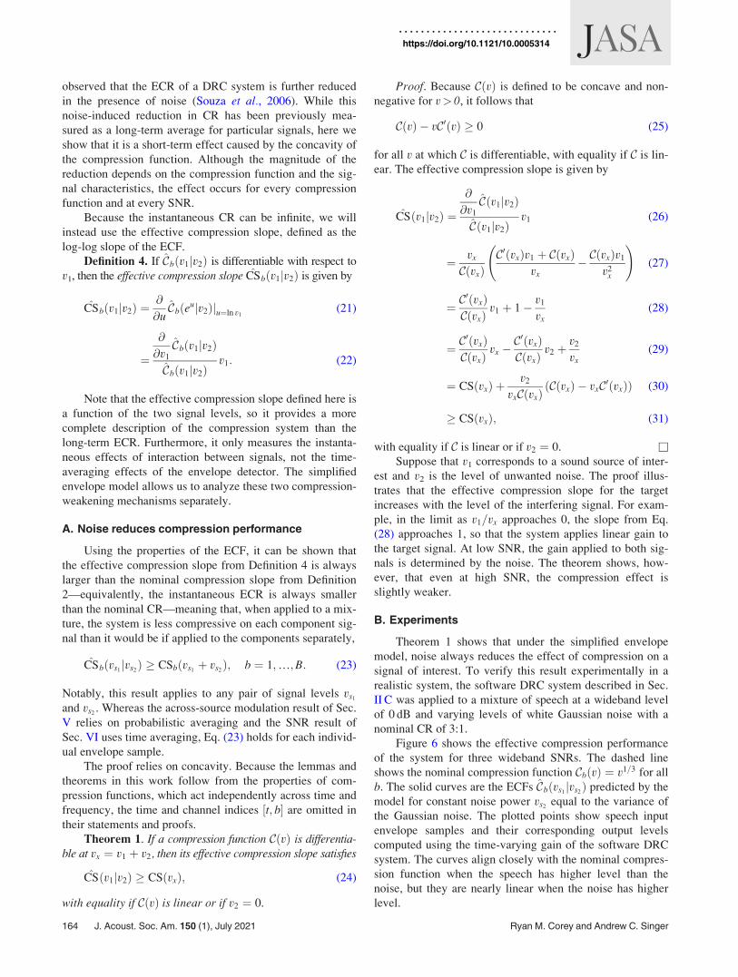
Figure 6 shows the effective compression performance

of the system for three wideband SNRs. The dashed line

shows the nominal compression function CbðvÞ ¼ v1=3 for all

b. The solid curves are the ECFs Cbðvs1jvs2Þ predicted by the

model for constant noise power vs2equal to the variance of

the Gaussian noise. The plotted points show speech input

envelope samples and their corresponding output levels

computed using the time-varying gain of the software DRC

system. The curves align closely with the nominal compres-

sion function when the speech has higher level than the

noise, but they are nearly linear when the noise has higher

level.

164 J. Acoust. Soc. Am. 150 (1), July 2021 Ryan M. Corey and Andrew C. Singer

https://doi.org/10.1121/10.0005314

The long-term ECR depends on the distribution of

envelope samples. For target signals whose envelopes are

usually above the noise level, the long-term ECR will be

close to the nominal ratio. When the noise is usually more

intense, as in the rightmost curve of Fig. 6, the long-term

ECR will be close to unity. Using the method of Souza et al.(2006), which measures dynamic range between the 5th and

95th percentiles of input and output envelope samples, and

averaging across signal bands, the long-term ECRs from the

experiments here were 1.01 at –30 dB SNR, 1.17 at 0 dB,

and 1.75 at þ30 dB.

V. ACROSS-SOURCE MODULATION DISTORTION

DRC creates distortion in mixtures because the pres-

ence of one signal alters the gain applied to another signal.

It has been observed experimentally (Alexander and

Masterson, 2015; Stone and Moore, 2004, 2007, 2008) that

when two signals are mixed together and passed through a

compressor, their output envelopes become negatively cor-

related: As one sound becomes louder, the other sound

becomes quieter. The across-source modulation coeffient, a

measure of this negative correlation, was found to be corre-

lated with reduced speech intelligibility (Stone and Moore,

2007, 2008).

A. Output levels are anticorrelated

The ECF can be used to show that if the input envelopes

vs1½t; b� and vs2

½t; b� are independent random processes, then

the covariance between the output levels in each channel is

negative,

Covðvr1t; b½ �; vr2

t; b½ �Þ � 0; b ¼ 1;…;B: (32)

The covariance is an ensemble mean over the distributions

of the envelope samples vr1½t; b� and vr2

½t; b�. Although the

covariance is often measured empirically using a time aver-

age, our mathematical analysis applies to each time index

and channel independently.

We first show that the ECF is nondecreasing in one

envelope and nonincreasing in the other.

Lemma 1. Any ECF Cðv1jv2Þ is nondecreasing in v1

and nonincreasing in v2 for v1; v2 � 0.

Proof. Because CðvÞ is nondecreasing and v2 is non-

negative, Cðv1jv2Þ ¼ Cðv1 þ v2Þðv1=v1 þ v2Þ is the product

of two nondecreasing functions of v1 and is therefore nonde-

creasing. Because CðvÞ is concave and non-negative, CðvÞ=vis nonincreasing for v> 0. Then Cðv1 þ v2Þ=ðv1 þ v2Þ is non-

increasing in v2. �

Next, we will need the following result about functions

of random variables. Let E denote the expectation of a ran-

dom variable, that is, its probabilistic mean.

Lemma 2. If f(x) is nondecreasing, g(x) is nonincreas-

ing, X is a random variable, and E½f ðXÞ�; E½gðXÞ�, and

E½f ðXÞgðXÞ� exist, then

E f ðXÞgðXÞ½ � � E f ðXÞ½ �E gðXÞ½ �: (33)

Proof. See Appendix A. �

We can now prove that independent envelopes become

negatively correlated when compressed.

Theorem 2. If Cðv1jv2Þ is an ECF and V1 and V2 areindependent random variables, then

Cov CðV1jV2Þ; CðV2jV1Þ� �

� 0: (34)

Proof. Because CovðCðV1jV2Þ; CðV2jV1ÞÞ ¼ E½CðV1jV2ÞCðV2jV1Þ� �E½CðV1jV2Þ�E½CðV2jV1Þ�, it is sufficient to

show that

E CðV1jV2ÞCðV2jV1Þh i

� E CðV1jV2Þh i

E CðV2jV1Þh i

:

(35)

From Lemma 1, Cðv1jv2Þ is a nondecreasing function of v1

and a nonincreasing function of v2. Let E½XjY� denote the

conditional expectation of X given Y. From iterated expecta-

tion and application of Lemma 2, we have

E CðV1jV2ÞCðV2jV1Þh i¼ EV2

EV1CðV1jV2ÞCðV2jV1ÞjV2

h ih i(36)

� EV2EV1

CðV1jV2ÞjV2

h iEV1

CðV2jV1ÞjV2

h ih i: (37)

Now, because V1 and V2 are independent, EV1½CðV1jV2ÞjV2�

is a nonincreasing function of V2 and EV1½CðV2jV1ÞjV2� is a

nondecreasing function of V2. Applying Lemma 2 once

more,

E CðV1jV2ÞCðV2jV1Þh i

�EV2EV1

CðV1jV2ÞjV2

h ih i�EV2

EV1CðV2jV1ÞjV2

h ih i(38)

¼ E CðV1jV2Þh i

E CðV2jV1Þh i

:

(39)�

For linear gain, the theorem holds with equality because

Cðv1jv2Þ does not depend on v2. The magnitude of the negative

correlation depends on the compression function: Stronger

FIG. 6. (Color online) ECF for speech and white noise at different wide-

band input SNRs. The dashed line shows the nominal compression function,

the curves show the ECFs evaluated with constant noise level, and the plot-

ted points show speech envelope samples.

J. Acoust. Soc. Am. 150 (1), July 2021 Ryan M. Corey and Andrew C. Singer 165

https://doi.org/10.1121/10.0005314

compression causes the ECFs and the conditional expectations

to increase or decrease more quickly, resulting in a stronger

negative correlation. The channel structure and time constants

of the envelope detector affect the correlation indirectly by

altering the distributions of V1 and V2.

B. Experiments

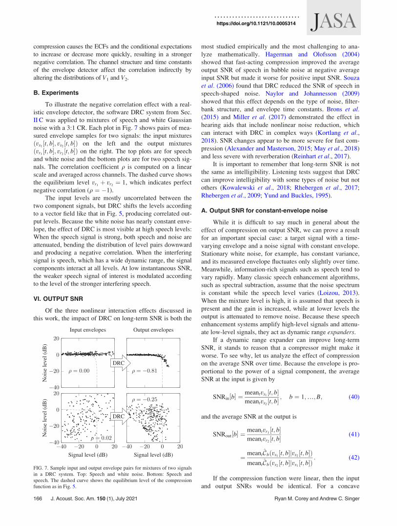
To illustrate the negative correlation effect with a real-

istic envelope detector, the software DRC system from Sec.

II C was applied to mixtures of speech and white Gaussian

noise with a 3:1 CR. Each plot in Fig. 7 shows pairs of mea-

sured envelope samples for two signals: the input mixtures

ðvs1½t; b�; vs2

½t; b�Þ on the left and the output mixtures

ðvr1½t; b�; vr2

½t; b�Þ on the right. The top plots are for speech

and white noise and the bottom plots are for two speech sig-

nals. The correlation coefficient q is computed on a linear

scale and averaged across channels. The dashed curve shows

the equilibrium level vr1þ vr2

¼ 1, which indicates perfect

negative correlation (q ¼ �1).

The input levels are mostly uncorrelated between the

two component signals, but DRC shifts the levels according

to a vector field like that in Fig. 5, producing correlated out-

put levels. Because the white noise has nearly constant enve-

lope, the effect of DRC is most visible at high speech levels:

When the speech signal is strong, both speech and noise are

attenuated, bending the distribution of level pairs downward

and producing a negative correlation. When the interfering

signal is speech, which has a wide dynamic range, the signal

components interact at all levels. At low instantaneous SNR,

the weaker speech signal of interest is modulated according

to the level of the stronger interfering speech.

VI. OUTPUT SNR

Of the three nonlinear interaction effects discussed in

this work, the impact of DRC on long-term SNR is both the

most studied empirically and the most challenging to ana-

lyze mathematically. Hagerman and Olofsson (2004)

showed that fast-acting compression improved the average

output SNR of speech in babble noise at negative average

input SNR but made it worse for positive input SNR. Souza

et al. (2006) found that DRC reduced the SNR of speech in

speech-shaped noise. Naylor and Johannesson (2009)

showed that this effect depends on the type of noise, filter-

bank structure, and envelope time constants. Brons et al.(2015) and Miller et al. (2017) demonstrated the effect in

hearing aids that include nonlinear noise reduction, which

can interact with DRC in complex ways (Kortlang et al.,2018). SNR changes appear to be more severe for fast com-

pression (Alexander and Masterson, 2015; May et al., 2018)

and less severe with reverberation (Reinhart et al., 2017).

It is important to remember that long-term SNR is not

the same as intelligibility. Listening tests suggest that DRC

can improve intelligibility with some types of noise but not

others (Kowalewski et al., 2018; Rhebergen et al., 2017;

Rhebergen et al., 2009; Yund and Buckles, 1995).

A. Output SNR for constant-envelope noise

While it is difficult to say much in general about the

effect of compression on output SNR, we can prove a result

for an important special case: a target signal with a time-

varying envelope and a noise signal with constant envelope.

Stationary white noise, for example, has constant variance,

and its measured envelope fluctuates only slightly over time.

Meanwhile, information-rich signals such as speech tend to

vary rapidly. Many classic speech enhancement algorithms,

such as spectral subtraction, assume that the noise spectrum

is constant while the speech level varies (Loizou, 2013).

When the mixture level is high, it is assumed that speech is

present and the gain is increased, while at lower levels the

output is attenuated to remove noise. Because these speech

enhancement systems amplify high-level signals and attenu-

ate low-level signals, they act as dynamic range expanders.

If a dynamic range expander can improve long-term

SNR, it stands to reason that a compressor might make it

worse. To see why, let us analyze the effect of compression

on the average SNR over time. Because the envelope is pro-

portional to the power of a signal component, the average

SNR at the input is given by

SNRin b½ � ¼ meantvs1t; b½ �

meantvs2t; b½ � ; b ¼ 1;…;B; (40)

and the average SNR at the output is

SNRout b½ � ¼ meantvr1t; b½ �

meantvr2t; b½ � (41)

¼ meantCbðvs1t; b½ �jvs2

t; b½ �ÞmeantCbðvs2

t; b½ �jvs1t; b½ �Þ

: (42)

If the compression function were linear, then the input

and output SNRs would be identical. For a concave

FIG. 7. Sample input and output envelope pairs for mixtures of two signals

in a DRC system. Top: Speech and white noise. Bottom: Speech and

speech. The dashed curve shows the equilibrium level of the compression

function as in Fig. 5.

166 J. Acoust. Soc. Am. 150 (1), July 2021 Ryan M. Corey and Andrew C. Singer

https://doi.org/10.1121/10.0005314

compression function with convex gain, it can be shown

that, if the noise envelope is constant, then the average out-

put SNR is lower than the average input SNR,

SNRout b½ � � SNRin b½ �; b ¼ 1;…;B: (43)

Unlike in Sec. V, here the envelopes are not modeled as ran-

dom processes and the quantities of interest are time aver-

ages, not ensemble averages.

The proofs in this section rely on an additional technical

condition on the compression function. Not only must CbðvÞbe non-negative and concave, the gain function CbðvÞ=vmust be convex. This condition is satisfied for many smooth

compression functions, including linear, power-law, and

logarithmic, but not for some functions with corners like

that in Fig. 2. This condition ensures that the ECF is con-

cave in its first argument and convex in its second.

Lemma 3. If CðvÞ is a compression function and CðvÞ=vis convex for all v> 0, then the ECF Cðv1jv2Þ is concave in

v1 and convex in v2.

Proof. See Appendix B. �

This property lets us take advantage of Jensen’s

inequality (Cover and Thomas, 2006), one form of which

states that for any convex function f(x),

meant f ðx t½ �Þ � f meantx t½ �ð Þ; (44)

with equality if f(x) is linear or x½t� is constant. The same

property holds with the inequality reversed if f(x) is a con-

cave function. Jensen’s inequality allows us to prove that

the average output SNR is no larger than the average input

SNR.

Theorem 3. If CðvÞ is a compression function andCðvÞ=v is convex for all v> 0, v1½t� > 0 for all t, and v2½t�¼ �v2 > 0 for all t, then

SNRout � SNRin (45)

with equality if v1½t� is constant or C is linear.Proof. Since v2½t� is fixed, the output SNR can be

written

SNRout ¼meantCðv1 t½ �j�v2ÞmeantCð�v2jv1 t½ �Þ

: (46)

The numerator is the mean over t of a concave function of

v1½t�. By Jensen’s inequality,

meantCðv1 t½ �j�v2Þ � Cðmeantv1 t½ �j�v2Þ; (47)

with equality when C is linear or v1½t� is constant. Similarly,

the denominator is the mean over t of a convex function of

v1½t�. Again applying Jensen’s inequality,

meantCð�v2jv1 t½ �Þ � Cð�v2jmeantv1 t½ �Þ; (48)

with equality when C is linear or v1½t� is constant. Let

�v1 ¼ meantv1½t�. Since the numerator and denominator of

Eq. (46) are both positive, we have

SNRout �Cð�v1j�v2ÞCð�v2j�v1Þ

(49)

¼ �v1Cð�v1 þ �v2Þ=ð�v1 þ �v2Þ�v2Cð�v1 þ �v2Þ=ð�v1 þ �v2Þ

(50)

¼ �v1

�v2

(51)

¼ SNRin; (52)

with equality when C is linear or v1½t� is constant. �

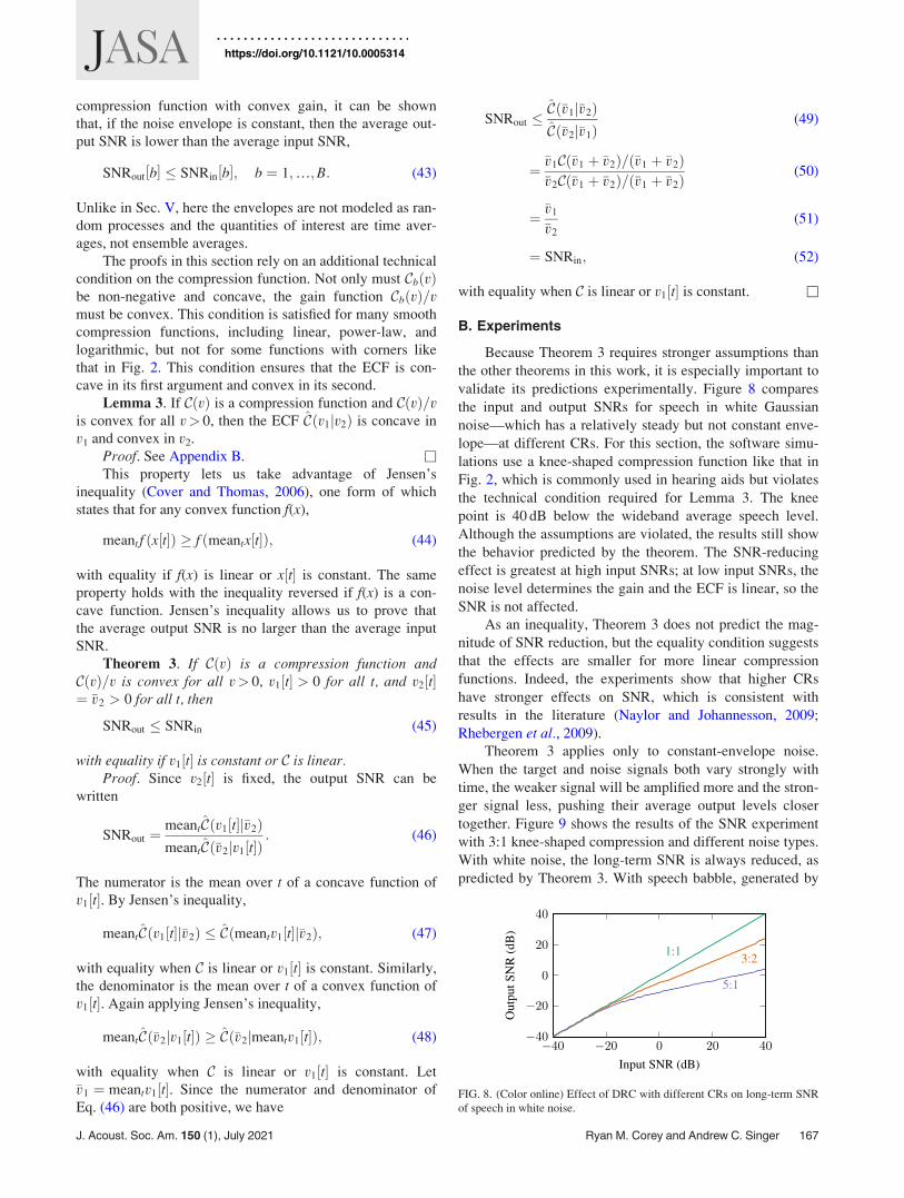
B. Experiments

Because Theorem 3 requires stronger assumptions than

the other theorems in this work, it is especially important to

validate its predictions experimentally. Figure 8 compares

the input and output SNRs for speech in white Gaussian

noise—which has a relatively steady but not constant enve-

lope—at different CRs. For this section, the software simu-

lations use a knee-shaped compression function like that in

Fig. 2, which is commonly used in hearing aids but violates

the technical condition required for Lemma 3. The knee

point is 40 dB below the wideband average speech level.

Although the assumptions are violated, the results still show

the behavior predicted by the theorem. The SNR-reducing

effect is greatest at high input SNRs; at low input SNRs, the

noise level determines the gain and the ECF is linear, so the

SNR is not affected.

As an inequality, Theorem 3 does not predict the mag-

nitude of SNR reduction, but the equality condition suggests

that the effects are smaller for more linear compression

functions. Indeed, the experiments show that higher CRs

have stronger effects on SNR, which is consistent with

results in the literature (Naylor and Johannesson, 2009;

Rhebergen et al., 2009).

Theorem 3 applies only to constant-envelope noise.

When the target and noise signals both vary strongly with

time, the weaker signal will be amplified more and the stron-

ger signal less, pushing their average output levels closer

together. Figure 9 shows the results of the SNR experiment

with 3:1 knee-shaped compression and different noise types.

With white noise, the long-term SNR is always reduced, as

predicted by Theorem 3. With speech babble, generated by

FIG. 8. (Color online) Effect of DRC with different CRs on long-term SNR

of speech in white noise.

J. Acoust. Soc. Am. 150 (1), July 2021 Ryan M. Corey and Andrew C. Singer 167

https://doi.org/10.1121/10.0005314

mixing 14 VCTK speech clips, the SNR is slightly increased

at low input SNRs. When the target and interference signals

are both single-talker speech signals, the long-term SNR is

improved when it is negative but made worse when it is

positive.

These results align well with those in the literature.

Hagerman and Olofsson (2004) showed that fast-acting com-

pression can improve negative SNRs but worsen SNRs near

zero for speech in babble noise. Naylor and Johannesson

(2009) found that output SNR is always reduced for speech

in unmodulated noise, greatly reduced at positive input SNR

and slightly reduced at negative input SNR for speech in

modulated noise, and symmetrically increased at negative

input SNR and decreased at positive input SNR for a mixture

of two speech signals. Reinhart et al. (2017) performed

experiments with different numbers of talkers and found that

the SNR improvement at negative input SNRs declined with

each additional interfering talker, consistent with the results

for speech babble here.

VII. DISCUSSION

The mathematical analysis presented here confirms the

empirical evidence from the hearing literature that DRC

causes unintended distortion in noise. The effects of this dis-

tortion depend on the characteristics of the signals, espe-

cially their relative levels. At low SNR, the ECF for the

target signal becomes nearly linear and the dynamic range

of that signal is not changed. At high SNR, the signal of

interest is amplified by less than the noise, reducing average

SNR. At all SNRs, the signal components modulate each

other, compressing the weaker signal according to the level

of the stronger component.

The theorems in this work apply to ideal envelopes that

obey the additivity assumption. In that sense, they are opti-

mistic predictions. Real DRC systems that use measured

envelopes would exhibit even stronger interactions between

signals. Further theoretial work is required to model distor-

tion within the envelope detector, predict the effects of fil-

terbank structure and envelope time constants, and show

how these nonlinearities interact with those of the compres-

sion function.

Can anything be done to improve the performance of

DRC systems in noise? The analysis shows that all these

effects are caused by the concave curvature of the

compression function, which is also what makes the system

compressive. The results for effective compression perfor-

mance and across-source modulation hold instantaneously,

not just over time, and apply to any compression function

and any combination of signals, even hypothetical ideal sig-

nals that have independent envelopes. It seems, then, that

nonlinear interactions are inevitable whenever signals are

compressed as a mixture.

A possible solution is to compress the component sig-

nals of a mixture independently, as music producers do

when mixing instrumental and vocal recordings. Listening

tests have shown improved intelligibility when signals are

compressed before rather than after mixing (Rhebergen

et al., 2009; Stone and Moore, 2008). Of course, real hear-

ing aids do not have access to the unmixed source signals,

so a practical multisource compression system must perform

source separation. Hassager et al. (2017) used a single-

microphone classification method to separate direct from

reverberant signal components, helping to preserve spatial

cues that can be distorted by DRC. May et al. (2018) pro-

posed a single-microphone separation system that applies

fast-acting compression to speech components and slow-

acting compression to noise components; listening experi-

ments with an ideal separation algorithm improved both

quality and intelligibility (Kowalewski et al., 2020). Corey

and Singer (2017) used a multimicrophone separation

method to apply separate compression functions to each of

several competing speech signals. The output exhibited bet-

ter measures of across-source modulation distortion, effec-

tive compression performance, and SNR compared to a

conventional system. The modeling framework described

here could be applied to analyze the performance of these

multisource compression systems and to devise new ones.

VIII. CONCLUSIONS

The mathematical tools introduced in this work can

help researchers to understand the distortion effects of con-

ventional DRC systems in noise and to devise new

approaches to nonlinear processing for mixtures of multiple

signals. The additive envelope model allows the envelope

detector and compression function to be analyzed indepen-

dently, greatly reducing the complexity of the system. The

ECF models interactions between signal envelopes at the

input and output of any compression function, characteriz-

ing system behavior across all signal levels. It can be used

to analyze instantaneous interactions or integrated into long-

term or probabilistic models to study average effects.

Like the human auditory system itself, DRC is a com-

plex nonlinear system that defies simple analysis. By model-

ing how DRC systems behave in the presence of noise, we

can develop and analyze new strategies for nonlinear signal

processing in the most challenging environments.

ACKNOWLEDGMENTS

This research was supported by the National Science

Foundation under Grant No. 1919257 and by an

FIG. 9. (Color online) Effect of compression on long-term SNR of mixtures

of speech with different types of noise.

168 J. Acoust. Soc. Am. 150 (1), July 2021 Ryan M. Corey and Andrew C. Singer

https://doi.org/10.1121/10.0005314

appointment to the Intelligence Community Postdoctoral

Research Fellowship Program at the University of Illinois

Urbana-Champaign, administered by Oak Ridge Institute

for Science and Education through an interagency

agreement between the U.S. Department of Energy and the

Office of the Director of National Intelligence.

APPENDIX A: PROOF OF LEMMA 2

Lemma 2. If f(x) is nondecreasing, g(x) is nonincreas-

ing, X is a random variable, and E½f ðXÞ�; E½gðXÞ�, and

E½f ðXÞgðXÞ� exist, then

E f ðXÞgðXÞ½ � � E f ðXÞ½ �E gðXÞ½ �: (A1)

Proof. Because f(x) is nondecreasing and g(x) is nonincreas-

ing, for every x and y we have

f ðxÞ � f ðyÞ½ � gðxÞ � gðyÞ½ � � 0: (A2)

It is sufficient to show that E½f ðXÞgðXÞ� �E½f ðXÞ�E½gðXÞ� � 0. If X has cumulative distribution function P(x),

then

E f ðXÞgðXÞ½ ��E f ðXÞ½ �E gðXÞ½ �

¼ð

x

f ðxÞgðxÞdPðxÞ�ð

x

f ðxÞdPðxÞð

y

gðyÞdPðyÞ (A3)

¼ð

x

ðy

f ðxÞ gðxÞ � gðyÞ½ � dPðyÞdPðxÞ (A4)

¼ð

x

ðy<x

f ðxÞ gðxÞ � gðyÞ½ � dPðyÞdPðxÞ

þð

y

ðx<y

f ðxÞ gðxÞ � gðyÞ½ � dPðxÞdPðyÞ (A5)

¼ð

x

ðy<x

f ðxÞ gðxÞ � gðyÞ½ � dPðyÞdPðxÞ

þð

x

ðy<x

f ðyÞ gðyÞ � gðxÞ½ � dPðyÞdPðxÞ (A6)

¼ð

x

ðy<x

f ðxÞ� f ðyÞ½ � gðxÞ� gðyÞ½ �dPðyÞdPðxÞ (A7)

� 0: (A8)

Equation (A5) swaps the order of integration using Fubini’s

theorem (Knapp, 2005) and line Eq. (A6) exchanges the

integration variables x and y. �

APPENDIX B: PROOF OF LEMMA 3

Lemma 3. If CðvÞ is a compression function and CðvÞ=vis convex for all v> 0, then the ECF Cðv1jv2Þ is concave in

v1 and convex in v2.

Proof. Starting with Definition 3 and letting

v1 ¼ kpþ ð1� kÞq,

Cðv1jv2Þ ¼Cðkpþ ð1� kÞqþ v2Þkpþ ð1� kÞqþ v2

ðkpþ ð1� kÞqÞ

(B1)

¼ Cðkðpþ v2Þ þ ð1� kÞðqþ v2ÞÞ (B2)

� v2

Cðkðpþ v2Þ þ ð1� kÞðqþ v2ÞÞkðpþ v2Þ þ ð1� kÞðqþ v2Þ

: (B3)

Because CðvÞ is concave and CðvÞ=v is convex,

Cðv1jv2Þ � kCðpþ v2Þ þ ð1� kÞCðqþ v2Þ (B4)

� v2 kCðpþ v2Þ

pþ v2

þ ð1� kÞ Cðqþ v2Þqþ v2

� �(B5)

¼ kCðpþ v2Þ

pþ v2

pþ ð1� kÞ Cðqþ v2Þqþ v2

(B6)

¼ kCðpjv2Þ þ ð1� kÞCðqjv2Þ: (B7)

Therefore, Cðv1jv2Þ is concave in v1.

Similarly, letting v2 ¼ kpþ ð1� kÞq,

Cðv1jv2Þ ¼Cðv1 þ kpþ ð1� kÞqÞv1 þ kpþ ð1� kÞq v1 (B8)

¼ Cðkðv1 þ pÞ þ ð1� kÞðv1 þ qÞÞkðv1 þ pÞ þ ð1� kÞðv1 þ qÞ v1 (B9)

� kCðv1 þ pÞv1 þ p

v1 þ ð1� kÞ Cðv1 þ qÞv1 þ q

v1 (B10)

¼ kCðv1jpÞ þ ð1� kÞCðv1jqÞ: (B11)

Therefore, Cðv1jv2Þ is convex in v2. �

Alexander, J. M., and Masterson, K. (2015). “Effects of WDRC release

time and number of channels on output SNR and speech recognition,” Ear

Hear. 36(2), e35–e49.

Alexander, J. M., and Rallapalli, V. (2017). “Acoustic and perceptual

effects of amplitude and frequency compression on high-frequency

speech,” J. Acoust. Soc. Am. 142(2), 908–923.

Allen, J. B. (2003). “Amplitude compression in hearing aids,” in MITEncyclopedia of Communication Disorders, edited by R. Kent (MIT

Press, Cambridge, MA), pp. 413–423.

ANSI (1996). ANSI S3.22-1996, Specification of Hearing AidCharacteristics (ANSI, New York).

Braida, L., Durlach, N., De Gennaro, S., Peterson, P., Bustamante, D.,

Studebaker, G., and Bess, F. (1982). “Review of recent research on multi-

band amplitude compression for the hearing impaired,” in The VanderbiltHearing Aid Report, edited by G. Studebaker and F. H. Bess (York Press,

London).

Brons, I., Houben, R., and Dreschler, W. A. (2015). “Acoustical and per-

ceptual comparison of noise reduction and compression in hearing aids,”

J. Speech Lang. Hear. Res. 58(4), 1363–1376.

Corey, R. M., and Singer, A. C. (2017). “Dynamic range compression for

noisy mixtures using source separation and beamforming,” in IEEEWorkshop on Applications of Signal Processing to Audio and Acoustics(WASPAA), October 15–18, New Paltz, NY.

Cover, T. M., and Thomas, J. A. (2006). Elements of Information Theory(Wiley, New York).

Giannoulis, D., Massberg, M., and Reiss, J. D. (2012). “Digital dynamic

range compressor design—A tutorial and analysis,” J. Audio Eng. Soc.

60(6), 399–408.

J. Acoust. Soc. Am. 150 (1), July 2021 Ryan M. Corey and Andrew C. Singer 169

https://doi.org/10.1121/10.0005314

Hagerman, B., and Olofsson, A. (2004). “A method to measure the effect of

noise reduction algorithms using simultaneous speech and noise,” Acta

Acust. united Ac. 90(2), 356–361.

Hajek, B. (2015). Random Processes for Engineers (Cambridge University

Press, Cambridge, UK).

Hassager, H. G., May, T., Wiinberg, A., and Dau, T. (2017). “Preserving

spatial perception in rooms using direct-sound driven dynamic range

compression,” J. Acoust. Soc. Am. 141(6), 4556–4566.

Kates, J. M. (2005). “Principles of digital dynamic-range compression,”

Trends Amplif. 9(2), 45–76.

Kates, J. M. (2008). Digital Hearing Aids (Plural Publishing, London).

Knapp, A. W. (2005). Basic Real Analysis (Birkh€auser, Basel, Switzerland).

Kortlang, S., Chen, Z., Gerkmann, T., Kollmeier, B., Hohmann, V., and

Ewert, S. D. (2018). “Evaluation of combined dynamic compression and

single channel noise reduction for hearing aid applications,” Int. J.

Audiol. 57, S43–S54.

Kowalewski, B., Dau, T., and May, T. (2020). “Perceptual evaluation of

signal-to-noise-ratio-aware dynamic range compression in hearing aids,”

Trends Hear. 24, 233121652093053–233121652093014.

Kowalewski, B., Zaar, J., Fereczkowski, M., MacDonald, E. N., Strelcyk,

O., May, T., and Dau, T. (2018). “Effects of slow-and fast-acting com-

pression on hearing-impaired listeners’ consonant–vowel identification in

interrupted noise,” Trends Hear. 22,

233121651880087–233121651880012.

Loizou, P. C. (2013). Speech Enhancement: Theory and Practice (CRC

Press, Boca Raton, FL).

Ludvigsen, C. (1993). “The use of objective methods to predict the intelligi-

bility of hearing aid processed speech,” in Proceedings of the 15th

Danavox Symposium, December 15, 1993, Kolding, Denmark, pp. 81–94.

May, T., Kowalewski, B., and Dau, T. (2018). “Signal-to-noise-ratio-aware

dynamic range compression in hearing aids,” Trends Hear. 22,

233121651879090–233121651879012.

Miller, C. W., Bentler, R. A., Wu, Y.-H., Lewis, J., and Tremblay, K.

(2017). “Output signal-to-noise ratio and speech perception in noise:

Effects of Algorithm,” Int. J. Audiol. 56(8), 568–579.

Naylor, G., and Johannesson, R. B. (2009). “Long-term signal-to-noise ratio

at the input and output of amplitude-compression systems,” J. Am. Acad.

Audiol. 20(3), 161–171.

Plomp, R. (1988). “The negative effect of amplitude compression in multi-

channel hearing aids in the light of the modulation-transfer function,”

J. Acoust. Soc. Am. 83(6), 2322–2327.

Rallapalli, V. H., and Alexander, J. M. (2019). “Effects of noise and

reverberation on speech recognition with variants of a multichannel

adaptive dynamic range compression scheme,” Int. J. Audiol. 58(10),

661–669.

Reinhart, P., Zahorik, P., and Souza, P. E. (2017). “Effects of reverberation,

background talker number, and compression release time on signal-to-

noise ratio,” J. Acoust. Soc. Am. 142(1), EL130–EL135.

Rhebergen, K. S., Maalderink, T. H., and Dreschler, W. A. (2017).

“Characterizing speech intelligibility in noise after wide dynamic range

compression,” Ear Hear. 38(2), 194–204.

Rhebergen, K. S., Versfeld, N. J., and Dreschler, W. A. (2009). “The

dynamic range of speech, compression, and its effect on the speech recep-

tion threshold in stationary and interrupted noise,” J. Acoust. Soc. Am.

126(6), 3236–3245.

Salorio-Corbetto, M., Baer, T., Stone, M. A., and Moore, B. C. (2020).

“Effect of the number of amplitude-compression channels and compres-

sion speed on speech recognition by listeners with mild to moderate sen-

sorineural hearing loss,” J. Acoust. Soc. Am. 147(3), 1344–1358.

Souza, P. E. (2002). “Effects of compression on speech acoustics, intelligi-

bility, and sound quality,” Trends Amplif. 6(4), 131–165.

Souza, P. E., Jenstad, L. M., and Boike, K. T. (2006). “Measuring the

acoustic effects of compression amplification on speech in noise,”

J. Acoust. Soc. Am. 119(1), 41–44.

Stone, M. A., and Moore, B. C. (1992). “Syllabic compression: Effective

compression ratios for signals modulated at different rates,” British J.

Audiol. 26(6), 351–361.

Stone, M. A., and Moore, B. C. (2004). “Side effects of fast-acting dynamic

range compression that affect intelligibility in a competing speech task,”

J. Acoust. Soc. Am. 116(4), 2311–2323.

Stone, M. A., and Moore, B. C. (2007). “Quantifying the effects of fast-

acting compression on the envelope of speech,” J. Acoust. Soc. Am.

121(3), 1654–1664.

Stone, M. A., and Moore, B. C. (2008). “Effects of spectro-temporal mod-

ulation changes produced by multi-channel compression on intelligibil-

ity in a competing-speech task,” J. Acoust. Soc. Am. 123(2),

1063–1076.

Veaux, C., Yamagishi, J., and MacDonald, K. (2019). “CSTR VCTK cor-

pus: English multi-speaker corpus for CSTR voice cloning toolkit (ver-

sion 0.92),” University of Edinburgh Centre for Speech Technology

Research, https://datashare.ed.ac.uk/handle/10283/3443.

Villchur, E. (1973). “Signal processing to improve speech intelligibility in

perceptive deafness,” J. Acoust. Soc. Am. 53(6), 1646–1657.

Yund, E. W., and Buckles, K. M. (1995). “Enhanced speech perception at

low signal-to-noise ratios with multichannel compression hearing aids,”

J. Acoust. Soc. Am. 97(2), 1224–1240.

170 J. Acoust. Soc. Am. 150 (1), July 2021 Ryan M. Corey and Andrew C. Singer

https://doi.org/10.1121/10.0005314