Modeling of cryogenic sloshing including heat and mass transfer

A. van Foreest

German Aerospace Centre (DLR), Space Launcher System Analysis (SART), Institute of Space Systems, 28359 Bremen, Germany, Arnold.vanForeest@dlr.de

The paper discusses heat and mass transfer during sloshing of cryogenic liquids. Experiments have been executed to investigate this. The experimental results are analyzed and CFD tools are used to create a better understanding of the physical processes involved. A 1D engineering model has been set up with the goal to simulate the heat and transfer during sloshing with only very short CPU time (not more than a few minutes).

Nomenclature c = specific heat [J kg-1 K-1], or constant value f = frequency [Hz] g = gravitational acceleration [9.81 m s-2]

lhGr = modified Grashof number based on hl

2

lshQg

h = height [m] H = total height [m] L = latent heat of vaporization [J kg-1 K-1] m = mass [kg]

m = mass flow rate [kg s-1] M = molecular mass [kg mol-1] P = pressure [Pa] Pr = Prandtl number r = radius [m]

Q = heat input [W]

R = gas constant [J kg-1K-1]

R = universal gas constant [8.314 J·mol-1K-1] S = surface area [m2] t = time [s] T = temperature [K] V = volume [m3] x = x direction [m] z = z direction [m]

Greek symbols = coefficient of volumetric expansion [1/K]

= delta = correcting factor for the bulk gas motion [m·kg·J-1s-1] = conduction coefficient [W m-2 K-1] = density [kg m-3]

= accommodation coefficient [-] = kinematic viscosity [m2 s-1]

1

= dimensionless time 2lh

t

Sub/superscripts av = average value cd = conduction cv = convection f = fill i = ith node l = liquid ls = liquid surface new = new value p = pressurization, at constant pressure pch = phase change

s = surroundings sat = saturation v = vapor vap = vaporized Abbreviations AP = active pressurization 1D = one dimensional GN2 = gaseous nitrogen LH2 = liquid hydrogen LN2 = liquid nitrogen SP = self pressurization

2

1. Introduction lofo

shing in launch vehicle tanks can lead to undesired effects. Propellant sloshing creates lateral rces which have to be counteracted by the attitude control system. This dynamical behaviour of

sloshing has been extensively investigated. Abramson [1] developed analytical models which predict sloshing amplitude and frequency.

S Sloshing not only leads to undesired forces, but can also be responsible for undesired thermodynamic effects. This is especially the case when cryogenic propellants are used. For example sloshing of cryogenic liquids can lead to large pressure drops due to enhancement of the heat and mass transfer at the liquid-vapour interface. This effect has not been the subject of many studies. Because the problem is not well understood, cryogenic launch vehicle stages are designed with relatively large safety margins. A better understanding would lead to more efficient designs of cryogenic stages. For the development of future upper stages it is essential to understand this phenomenon better. To this end the Centre of Applied Space Technology and Microgravity (ZARM) in Bremen, Germany, has executed experiments for the investigation of cryogenic sloshing using LN2. Similar experiments have been executed by Moran et al.[2], Lacapere et al [3] and Das et al [4]. Moran et al. used LH2 and a spherical tank filled to different levels. Lacapere et al. used LOX and LN2 and a cylindrical tank and Das et al. used the non-cryogenic engineerg fluids FC-72 and HFE7000 and a cylindrical tank.

2. Experimental Setup The experiments involve a dewar made out of borosilicate glass. The space between the walls is evacuated to minimize heat transfer into the dewar by means of conduction and convection. The walls are silverized to minimize heat transfer by radiation. The dewar is filled with liquid nitrogen at ambient pressure. The cylindrical part of the dewar has a radius of r = 0.145 m. The dewar is filled to height Hf = 2r. The total height of the dewar is H = 0.65 m. The dewar is closed such that there is no contact of the inner part with the surroundings. Five temperature sensors are located in the liquid at heights of 0.003 m, 0.103 m, 0.203 m, 0.253 m and 0.278 m with respect to the dewar bottom. Two parallel sensor booms with 4 sensors each are located in the ullage. Sensors are located at 0.334 m 0.384 m 0.434 m and 0.484 m with respect to the dewar bottom. The test setup is illustrated in Figure 1. More detailed descriptions of the test setup can be found in [5]. A crank shaft introduces the lateral excitation of the dewar. The first natural sloshing frequency occurs at f = 1.8 Hz [5]. To avoid chaotic sloshing near this frequency but still have significant slosh amplitudes, an excitation frequency of 1.4 Hz is chosen and the excitation amplitude is set to 0.01 m. The dewar is pressurized by two different mechanisms. The first is by self-pressurisation and the second by active pressurisation. Self –pressurization test will be identified with “sp”, followed by a number indicating the maximum pressure during pressurization. Active pressurization test will be identified with “ap”, followed by a number indicating the maximum pressure during pressurization. In case of self-pressurisation the pressure will increase due to unavoidable heat leaks from the surroundings into the closed dewar. Heat input into the liquid due to unavoidable heat leaks from the surroundings can be determined using the temperature and pressure data. Total heat input during the stratification phase is determined to be 7 W, from which 6.3 W enters the liquid and 0.7 W the vapour. Active pressurization is achieved by actively adding gaseous nitrogen. The mass flow was set to 0.1 g/s, causing the pressure to increase much faster compared to the self-pressurization phase. During pressurization thermal layers will form in the liquid and ullage vapour. After a certain increase in pressure the dewar is exited laterally, causing the fluid to slosh.

3

Figure 1. Test Setup

3. Test Results

3.1. Pressure data Figure 2 shows the pressure measured during two of the self-pressurisation tests. During one of the tests, sloshing is initiated once the pressure has reached approximately 160 kPa.. This occurs after 3725 seconds. During sloshing the pressure decreases to 134.5 kPa. The minimum pressure is reached after 4420 seconds, 695 seconds after initialisation of the sloshing. During the other test, sloshing is initiated once the pressure has reached approximately 120 kPa. This occurs after 1078 seconds. During sloshing the pressure decreases to 113.5 kPa. The minimum pressure is reached after 1363 seconds, 285 seconds after initialisation of the sloshing.

4

100

110

120

130

140

150

160

170

0 500 1000 1500 2000 2500 3000 3500 4000 4500 5000 5500

time [s]

P [

kP

a]

P=150 kPa

P=120 kPa

Minimum Pressure 134.5kPa t= 4420 s ΔP=25.5 kPa

Start of sloshing t= 3725 s

Minimum Pressure 113.5 kPa t= 1363 s ΔP=8.3 kPa

Start of sloshing t= 1078 s

Figure 2. Pressure Development during Self-Pressurisation Tests. The triangular symbols correspond to a test where sloshing was initiated at a pressure of about 160 kPa, thecircular symbols correspond to a test where sloshing was initiated after the pressure had reached about 120 kPa.

Figure 3 shows the pressure measured during two of the active pressurisation tests. During one of the tests, sloshing is initiated once the pressure has reached approximately 160 kPa.. This occurs after 140 seconds. During sloshing the pressure decreases to 121.95 kPa. The minimum pressure is reached after 630 seconds, 490 seconds after initialisation of the sloshing. During the other test, sloshing is initiated once the pressure has reached approximately 120 kPa. This occurs after 40 seconds. During sloshing the pressure decreases to 117.1 kPa. The minimum pressure is reached after 188 seconds, 148 seconds after initialisation of the sloshing.

5

100

110

120

130

140

150

160

170

0 100 200 300 400 500 600 700time [s]

P [

kP

a]

P=160 kPa

P=120 kPa Minimum Pressure 121.95 kPa t= 630 s ΔP=38.4 kPa

Start of sloshing t=140 s

Start of sloshing t=40 s

Minimum Pressure 117.1kPa t= 188 s ΔP=7.8 kPa

Figure 3. Pressure Development during Active Pressurization Tests. The triangular symbols correspond to a test where sloshing was initiated at a pressure of about 160 kPa, the circular symbols correspond to a test where sloshing was initiated after the pressure had reached about 120 kPa.

An overview of the experimental results can be found in Table 1.

max

t

p[kPa/s

]

P [kPa] t [s]

(after slosh initiation)

sp160 -0.34 -25.5 695 sp120 -0.162 -8.3 285 ap160 -1.094 -38.4 490 ap120 -0.316 -7.8 148

Table 1. Results from sloshing experiments. “sp” stands for self-pressurization, “ap” for active pressurization. The numbers 160 and 120 stand for pressurization upto 160 kPa or 120 kPa. P is the maximum pressure drop which occurs during sloshing, t is the time it takes to reach minimum pressure after beginning of the sloshing.

6

3.2. Temperature in the ullage Temperature developments in the ullage measured during the two self-pressurization test are shown in Figure 4. Temperature increases graduately during the self-pressurization phase. When sloshing starts (indicated in the figure by a dashed line) the temperature at h = 0.334 m (the closest to the liquid surface) slightly drops. The temperatures in the other regions stay constant or increase only slightly.

0

20

40

60

80

100

120

140

160

180

200

0 500 1000 1500 2000 2500 3000 3500 4000 4500 5000 5500

time [s]

T [

K]

T1 h=0.484m

T2 h=0.434m

T3 h=0.384m

T4 h=0.334m

Figure 4. Temperature development in the ullage for the two self-pressurisation tests. The filled symbols represent the test with pressurisation up to 120 kPa. The open symbols represent the test with pressurisation to 160 kPa. The temperature measured by the sensor which is closest to the liquid surface shows a temperature drop after initiation of the sloshing. In the other areas the temperature does not change. Sloshing starts at the dotted lines.

Temperature developments in the ullage measured during the two active pressurization test are shown in Figure 5. Temperature increase during the active pressurization phase is much faster then compared to the self pressurization. When sloshing starts (indicated in the figure by a dashed line) the temperatures slightly drop.

7

0

20

40

60

80

100

120

140

160

180

200

220

0 100 200 300 400 500 600 700 800 900

time [s]

T [

K]

T1 h=0.484 m

T2 h=0.434 m

T3 h=0.384 m

T4 h=0.334 m

Figure 5. Temperature development in the ullage for the two active pressurisation tests. The filled symbols represent the test with pressurisation up to 120 kPa. The open symbols represent the test with pressurisation to 160 kPa. All temperature sensors show a slight decrease in temperature. The temperature closest to the liquid surface is most sensitive. Sloshing starts at the dotted lines.

3.3. Temperature development in the liquid Figure 6 and Figure 7 show the temperature distribution in the liquid at different times for the self-pressurisation and active pressurisation tests respectively. The temperatures at the liquid surface are assumed to be equal to the saturation temperature at the corresponding pressure. This saturation temperature is calculated using the Clausius-Clapyron equation [6]. For each test 3 instances in time are depicted, namely at the beginning of the test (t=0s), right before initiation of the sloshing and at minimum pressure during sloshing. Right before initiation of the sloshing large thermal gradients exist in the upper liquid layer. The sloshing results in a destruction of the stratification in this region and consequently a temperature drop in the upper part of the liquid. The temperature at the liquid surface is reduced, and thermodynamic equilibrium is broken. The ullage pressure is higher than the saturation pressure belonging to the liquid temperature at the liquid surface and this leads to condensation of ullage gas resulting in a pressure drop. This condensation procedure is reflected in the phase change model based on kinetic theory [7], where the liquid and vapour temperatures at the liquid-vapour interface have been assumed to be equal:

)(2

sec vsatl

lslshangepha pp

TR

MSm

(1)

A short analysis of following [7] results in ≈1.

8

Because is a function of temperature (the relation between and the liquid temperature can

for example be described by the Clausius-Clapyron equation) it will drop as temperature decreases. Once

the thermal equilibrium is broken the vapour pressure will be higher than . This will result in a

negative which means condensation will occur.

satlp

vapm

satlp lT

vp satlp

0

0.05

0.1

0.15

0.2

0.25

0.3

0.35

77 77.5 78 78.5 79 79.5 80 80.5 81 81.5 82

T [K]

h [

m]

t=0 s sp160

t=3725 s (Pmax) sp160

t=4420 s (Pmin during slosh) sp160

t=0 s sp120

t=1078 s (Pmax) sp120

t=1362 s (Pmin during slosh) sp120

liquid surface

Figure 6. Temperature in the liquid for the Self-Pressurization (sp) tests. The closed symbols correspond to the test with a maximum pressure of 160 kPa. The open symbols to the one with a maximum pressure of 120 kPa. The circles correspond to the temperatures at the beginning of the test, the squares indicate the temperatures at maximum pressure and the triangles correspond to the temperatures measured at minimum pressure during sloshing. The temperatures at the liquid surface are assumed to be equal to the saturation temperature of the corresponding pressure.

9

0

0.05

0.1

0.15

0.2

0.25

0.3

0.35

77 77.5 78 78.5 79 79.5 80 80.5 81 81.5 82

T [K]

h [

m]

t=0 s ap160

t=140 s (Pmax) ap160

t=630 s (Pmin during slosh) ap160

t=0 s ap120

t=40 s (Pmax) ap120

t=188 s (Pmin during slosh) ap120

liquid surface

Figure 7. Temperature in the liquid for the Active Pressurisation (ap) tests. The closed symbols correspond to the test with a maximum pressure of 160 kPa. The open symbols correspond to the one with a maximum pressure of 120 kPa. The circles correspond to the temperatures at the beginning of the test, the squares indicate the temperatures at maximum pressure and the triangles correspond to the temperatures measured at minimum pressure during sloshing. The temperatures at the liquid surface are assumed to be equal to the saturation temperature of the corresponding pressure.

From Figure 2, Figure 3, Figure 6 and Figure 7 it can be concluded that the stratification in the liquid before sloshing largely determines the pressure response during sloshing. If, for example the pressure responses of AP160 and SP160 are compared, it can be seen that the pressure response of AP160 is much stronger. The pressure drops faster and the minimum pressure which is reached during sloshing is also lower. The only parameter which is different for these experiments is the thermal gradient in the liquid. The same can be concluded when comparing AP120 with SP120. The thermal gradient in the liquid is the most important factor describing pressure drop. Therefore, the first step in developing a model for the prediction of pressure drop in a tank is to develop a model which predicts the liquid stratification.

10

4. CFD modeling of the stratification process

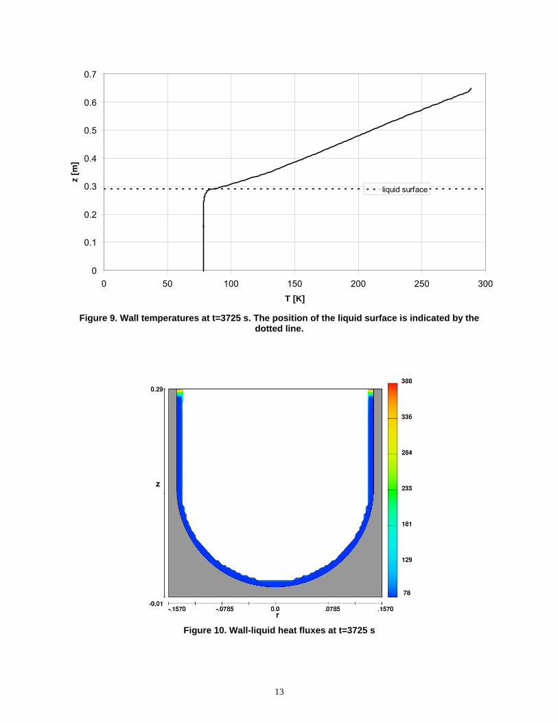
The stratification process has been modeled using the commercially available code FLOW 3D. A full conduction mode has been set up, thus taking into account conductive heat flow through the dewar wall. To be able to account for phase changes at the liquid surface, the phase change model has been switched on. A 2D 45x185 cell cylindrical mesh was used, taking into account symmetry along the z-axis. CPU time was approximately 44 hours on a single core 2.16 GHz processor. In Figure 8 the temperatue in the liquid during the stratification process is visible. It can clearly be seen that due to heat entering the liquid via the dewar wall, a thermal boundary layer at the wall develops. The heated liquid in this boundary layer then rises to the liquid surface, creating a pocket of warm liquid at the liquid surface. The pocket volume increases over time and after 300 s the complete liquid region is heated. In the middle of the bottom of the dewar a column of warm liquid builds up, also transporting warmer liquid to the liquid surface. At the liquid surface, a strong thermal gradient is visible, which increases over time. At 3725 s (the end of the stratification phase) the gradient has reached a maximum. Temperature at the liquid surface has reached 80.63 K, bulk liquid temperature lies at 78 K. The strong thermal gradient is caused by heat conducted tangential through the dewar wall. Conductive heat flow in this direction develops because of the much higher wall temperature in the warmer ullage region, as can be seen in Figure 9. This heat enters the liquid near the liquid surface, causing the thermal gradient. This is visible in Figure 10, where it can be seen very clearly that near the liquid surface, heat fluxes are more than 4 times as high as below the liquid surface. There will also be some heat transfer between liquid and vapor over the liquid vapor interface. As long as the vapor is at rest, this heat transfer will be caused by conduction through the vapor. The conduction coefficient of GN2 is very low (0.025 W m-1K-1 @ 280 K, 0.0075 W m-1K-1 @ 78 K) and heat transfer can be neglected. In certain cases, the vapor may be in motion which could greatly enhance the heat transfer due to conductive heat transfer. According to the simulations of the experiments the vapor motion was not significant and heat transfer between vapor and liquid is neglected in further analysis. To summarize, three main heat transfer mechanisms play a role in the stratification process:

1. Heat transfer normal to the wall entering the liquid causes the formation of a thermal boundary layer which transports warm liquid to the liquid surface. The volume of heated liquid becomes bigger and after a certain time, all the liquid is heated by this mechanism and heating occurs homogeneously over the liquid

2. Heat transfer tangential to the wall caused by the temperature gradient in the wall across the liquid surface causes heating of the liquid right below the liquid surface. This results in a strong thermal gradient in the liquid at the surface

3. Heat transfer between the liquid and the warmer vapor. Numerical results suggest this is not significant in the present case because there is almost no convective motion of the vapor and the heat conduction coefficient of the vapor is very low.

4. At the liquid surface phase changes can occur due to changing liquid temperature (equation (1)). During phase change heat will be released/extracted at the liquid surface

In Figure 11 these 4 mechanisms are depicted schematically.

11

t=0 s t=50 s

t=100 s t=200 s

t=300 s t=3725 s

Figure 8. Development of thermal stratification in the liquid during a FLOW 3D simulation of experiment SP160.

12

0

0.1

0.2

0.3

0.4

0.5

0.6

0.7

0 50 100 150 200 250 300

T [K]

z [m

]

liquid surface

Figure 9. Wall temperatures at t=3725 s. The position of the liquid surface is indicated by the dotted line.

Figure 10. Wall-liquid heat fluxes at t=3725 s

13

Figure 11. Heat transfer mechanisms

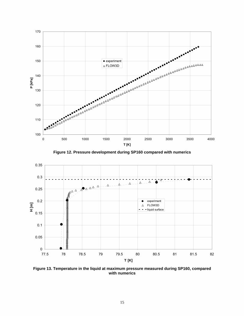
Due to the heating of the liquid, some liquid will evaporate according to equation (1). This will in turn result in a pressure increase in the dewar. Pressure developments according to the numerical model and according to the experiment are compared in Figure 12. As can be seen the pressure according to the numerical model is lower than the pressure measured during the experiment. In Figure 13 the temperatures in the liquid are compared. The black dots are the temperatures measured during the experiment. The temperature exactly at the liquid surface was not measured. Here it is assumed that the temperature at the liquid surface is equal to the saturation temperature belonging to the vapor pressure at this time. The temperature at the liquid surface according to the numerical model is lower. This is in line with the lower pressure. A possible explanation for these differences might be that the sensor boom, to which the temperature sensors were attached, is not taken into account in the numerical model. Additional heat conducted through this boom into the liquid might cause the liquid to heat up a bit more. One might also expect the meshing to be the cause of the problem. If the resolution is too small, the steep temperature gradient cannot be resolved. A mesh with 4 times as much cells was tried, but the results were the same so this option is ruled out.

Qwall_norm(1)

Qwall_norm(1)

Qull-prop(3)Qevap(4)Qwall_tan(2)

Qwall_norm(1)

Qwall_norm(1)

Qull-prop(3)Qevap(4)Qwall_tan(2)

Qwall_norm(1)

Qwall_norm(1)

Qull-prop(3)Qevap(4)Qwall_tan(2)

heatedh

lh

14

100

110

120

130

140

150

160

170

0 500 1000 1500 2000 2500 3000 3500 4000

T [K]

P [

kP

a]

experiment

FLOW3D

Figure 12. Pressure development during SP160 compared with numerics

0

0.05

0.1

0.15

0.2

0.25

0.3

0.35

77.5 78 78.5 79 79.5 80 80.5 81 81.5

T [K]

H [

m]

82

experiment

FLOW3D

liquid surface

Figure 13. Temperature in the liquid at maximum pressure measured during SP160, compared with numerics

15

5. A 1D model for the thermal stratification of the liquid The thermal gradient in the liquid which is present just before initiation of the sloshing is created by heat input into the liquid at the liquid surface. This causes the temperature of the liquid in the surface region to rise. As the temperature in the top liquid layer increases, a conductive heat flow through the liquid will cause the lower liquid regions to heat up as well and the thickness of this thermally heated region (thermal penetration depth) will increase over time. An energy equation can be set up for the thermal gradient in the liquid:

2

2

z

Tll

+ =inq

t

Tc l

lp

, (2)

where is the heat entering the liquid through the dewar wall. inq

The boundary condition is the heat added at the liquid surface which consists of heat which is transferred through the ullage vapour into the liquid and of heat released/extracted by a phase change at the liquid surface. This can be expressed by Fourier’s law:

vpch QQ

lsz

lsl z

T

(3)

where

pchQ Lm pch *

(4)

and can be calculated using equation pchm

(1). L is the latent heat of vaporization.

The above can be transferred into a 1D model. The liquid in the tank can be divided in a finite number of layers or nodes. Between each node conductive heat transfer can be calculated using a standard heat conduction equation:

icdQ

= lii

iii zz

TTS

1

1

(5)

The temperature increase in a layer can be calculated by:

newiT = iT dt

cm

QQQ

pi

inicdicd

1 (6)

In this equation, is the additional heat entering the liquid layer due to heat leaks from the

surroundings and, in case of the layer at the liquid surface, the heat entering due to phase change

and the heat entering due to heat exchange between vapor and liquid .

inQ

sQ

pchQ

vlQ

The four heat transfer mechanisms described in Figure 11 are inserted into the model as follows:

1. Heat transfer normal to the wall entering the liquid which causes the formation of a thermal boundary layer which transports warm liquid to the liquid surface can be modeled according to [8]:

72

32

32

2

Pr443.01Pr0924.0 lhl

llheated

Gr

R

hhhh

(7)

wher is the thickness of the heated volume and is the liquid height (see Figure 11).

The modified hof number depends on the heat flux entering the liquid. This heat flux has

e heatedh

Gras

lhlhGr

16

been determined from experimental and numerical data (using F OW 3D) and results in 3.8 W. The temperature of the heated volume can be calculated using:

L

bulkl

eated Th

QR

H

2

l

heated

h

h

hT

Pr

(8)

Based on the results of the numerical simulations, it is assumed that as soon as , the liquid

p uniformly. Heat transfer tangential to the wall causing heating of the liquid right below the liquid surface can

vapo tements it is known that the temperature distribution in the vapor is approximately

model

heatedh = lhheats u2.

be determined by assuming that ullage wall temperatures are equal to the r mperature. From the experilinear, with the highest temperature at the top of the dewar. Here, the temperature is approximately room temperature. At the liquid surface the vapor temperature is equal to the liquid temperature. Using the heat conduction coefficient for borosilicate (the dewar material) and the wall thickness (6mm) the heat conducted into the liquid can be estimated. This results in approximately 2.5 W. This heat is added to the liquid layer near the surface.

3. The heat transfer between vapor and liquid is set to zero for the present case 4. Heat exchange due to phase change can be determined using equations (1) and (4). This heat is

extracted from the layer at the liquid surface if liquid evaporates and added when vapour condensates. Pressure change in the dewar is calculated using the ideal gas RTP .

The temperature used is the average vapour temperature, which in the present case is about 170K.

Results of the 1D model are compared to experimental and the FLOW 3D numerical results in Figure 14 and Figure 15. As can be seen the 1D results and the FLOW 3D results are very close. CPU time for the

D model was le1 ss than a second. The time saving compared to the FLOW 3D CFD calculations (with a CPU time of 44 hours) is thus enormous.

100

110

120

130

140

150

160

170

1D model

experiment

FLOW3D

0 500 1000 1500 2000 2500 3000 3500 4000

T [K]

P [

kPa]

17

Figure 14. Pressure development according to experiment SP160, FLOW 3D and 1D model

0

0.05

0.1

0.15

0.2

0.25

0.3

0.35

77.5 78 78.5 79 79.5 80 80.5 81 81.5 82

T [K]

H [

m]

1D model

experiment

FLOW3D

liquid surface

Fi t

6. Pressure drop during sloshing During sloshing the thermal gradient is reduced, as explained in section 3.3. Due to convective flows, the heat transfer within the liquid is influenced. This can be modeled by an increase in the conduction coefficient in the liquid. An increase of conduction with a factor 47 results in a pressure drop shown in Figure 16. Temperature in the liquid is shown in Figure 17. Heat input from the surroundings into the liquid is increased by the sloshing motion so a correction for this has been applied in the 1D model. The model for the pressure drop is still under development but first results look very promising.

gure 15. Temperature in the liquid at t=3725s (right before sloshing) according to experimenSP160, FLOW 3D and 1D model

18

130

135

140

145

150

170

155

160

165experiment

1D model

3700 3900 4100 4300 4500 4700 4900 5100 5300 5500

time [s]

P [

Pa]

Figure 16. Pressure drop according to the 1D model compared to experimental values

0

0.05

0.1

0.15

0.2

0.25

0.3

77 77.5 78 78.5 79 79.5 80 80.5 81 81.5 82

T [K]

h [

m] t=3725 s (Pmax) sp160

t=4420 s (Pmin during slosh) sp160

T@Pmin, 1D model

T before slosh, 1D model

liquid surface

Figure 17. Temperature in the liquid at minimum pressure according to the 1D model compared to experimental values

19

7. Conclusions Experiments have been conducted which show that thermal stratification in a cryogenic liquid is the main cause for pressure drop during a sloshing motion. To be able to make fast engineering predictions of pressure drops during sloshing it is therefore necessary to first develop a reliable model for thermal stratification. Using the results of CFD simulations, a better understanding of the stratification process is created. Using this results a 1D engineering model has been developed which predicts the stratification quite accurate. The next step is to model the pressure drop. First analysis has shown that this can be modeled by increasing the thermal conductivity in the liquid. The pressure drop model is currently under development.

References [1] Abramson, H. N., "The Dynamic Behaviour of Liquids in Moving Containers" Tech. Report NASA-

SP-106, 1966. [2] Moran, E.M., McNeils, N.B., Kudlac, M.T., Haberbusch, M.S., Satornino, G.A.: Experimental

results of hydrogen slosh in a 60 cubic foot (1750 liter) tank. 30th Joint Propulsion Conference (1994), AIAA 94-3259

[3] Lacapere, J., Vieille, B., Legrand, B.: Experimental and numerical results of sloshing with cryogenic fluids, 2nd European Conference for Aerospace Sciences (EUCASS)

[4] Das, S. P., Hopfinger, E. J.: Mass transfer enhancement by gravity waves at a liquid vapour interface, Int. J. Heat Mass Tran., Vol. 52, No. 5-6 2009, pp. 1400-1411

[5] Arndt, T., Dreyer, M., Behruzi, P., Winter, M., Van Foreest, A.: Cryogenic Sloshing Tests in a

Pressurized Cylindrical Reservoir, Proceeding at the 45th AIAA Joint Propulsion Conference (2009), AIAA 2009-4860

[6] Baehr, H.D.: Thermodynamik, Springer, 1996 (German) [7] Carey, Van P.: Liquid-Vapor Phase-Change Phenomena: An Introduction to the Thermophysics

of Vaporization and Condensation Processes in Heat Transfer Equipment, Hemisphere Publishing Cooperation, 1992

[8] Chin, J.H. et.al..: Analytical and experimental study of liquid orientation and stratification in standard and reduced gravity fields, Lockheed missiles & space company, July 1964

20