modeling of activated sludge process by using …etd.lib.metu.edu.tr/upload/12605733/index.pdf ·...
TRANSCRIPT

MODELING OF ACTIVATED SLUDGE PROCESS BY USING
ARTIFICIAL NEURAL NETWORKS
A THESIS SUBMITTED TO THE GRADUATE SCHOOL OF NATURAL AND APPLIED SCIENCES
OF MIDDLE EAST TECHNICAL UNIVERSITY
BY
HAKAN MORAL
IN PARTIAL FULFILLMENT OF THE REQUIREMENTS FOR
THE DEGREE OF MASTER OF SCIENCE IN
ENVIRONMENTAL ENGINEERING
OCTOBER 2004

Approval of the Graduate School of Natural and Applied Sciences
___________________
Prof. Dr. Canan Özgen Director
I certify that this thesis satisfies all the requirements as a thesis for the degree of Master of Science.
___________________
Prof. Dr. Filiz B. Dilek
Head of Department
This is to certify that we have read this thesis and that in our opinion it is fully adequate, in scope and quality, as a thesis for the degree of Master of Science.
Assist. Prof. Dr. Ayegül Aksoy
Co-Supervisor
Prof. Dr. Celal F. Gökçay
Supervisor
Examining Committee Members
Prof Dr. Kahraman Ünlü (METU, ENVE) ___________________
Prof Dr. Celal F. Gökçay (METU, ENVE) ___________________
Assist. Prof Dr. Ayegül Aksoy (METU, ENVE) ___________________
Prof Dr. Filiz B. Dilek (METU, ENVE) ___________________
Assoc. Prof Dr. Gülen Güllü (HACETTEPE, ENVE) ___________________

iii
PLAGIARISM
I hereby declare that all information in this document has been obtained and
presented in accordance with academic rules and ethical conduct. I also declare that,
as required by these rules and conduct, I have fully cited and referenced all material
and results that are not original to this work.
Name, Last name: Hakan Moral
Signature

iv
ABSTRACT
MODELING OF ACTIVATED SLUDGE PROCESS BY USING ARTIFICIAL
NEURAL NETWORKS
Moral, Hakan
M.Sc., Department of Environmental Engineering
Supervisor: Prof. Dr. Celal F. Gökçay
Co-Supervior: Assist. Prof. Dr. Ayegül Aksoy
October 2004, 110 pages
Current activated sludge models are deterministic in character and are constructed
by basing on the fundamental biokinetics. However, calibrating these models are
extremely time consuming and laborious. An easy-to-calibrate and user friendly
computer model, one of the artificial intelligence techniques, Artificial Neural
Networks (ANNs) were used in this study. These models can be used not only
directly as a substitute for deterministic models but also can be plugged into the
system as error predictors.
Three systems were modeled by using ANN models. Initially, a hypothetical
wastewater treatment plant constructed in Simulation of Single-Sludge Processes for
Carbon Oxidation, Nitrification & Denitrification (SSSP) program, which is an
implementation of Activated Sludge Model No 1 (ASM1), was used as the source of
input and output data. The other systems were actual treatment plants, Ankara
Central Wastewater Treatment Plant, ACWTP and skenderun Wastewater
Treatment Plant (IskWTP).

v
A sensitivity analysis was applied for the hypothetical plant for both of the model
simulation results obtained by the SSSP program and the developed ANN model.
Sensitivity tests carried out by comparing the responses of the two models indicated
parallel sensitivities. In hypothetical WWTP modeling, the highest correlation
coefficient obtained with ANN model versus SSSP was about 0.980.
By using actual data from IskWTP the best fit obtained by the ANN model yielded
R value of 0.795 can be considered very high with such a noisy data. Similarly,
ACWTP the R value obtained was 0.688, where accuracy of fit is debatable.
Keywords: activated sludge process, artificial intelligence, artificial neural network,
modeling.

vi
ÖZ
AKTF ÇAMUR PROSESNN YAPAY SNR ALARI KULLANILARAK
MODELLENMES
Moral, Hakan
Y.Lisans, Çevre Mühendislii Bölümü
Tez Yöneticisi: Prof. Dr. Celal F. Gökçay
Ortak Tez Yöneticisi: Y. Doç. Dr. Ayegül Aksoy
Ekim 2004, 110 sayfa
Günümüz aktif çamur modelleri belirleyici karakterlidir ve temel biyokinetiklere
dayanarak kurulmulardır. Fakat bu modellerin kalibrasyonu fazlasıyla zaman alıcı
ve zahmetlidir. Bu çalımada, aktif çamur iletmelerinin kontrolü için yapay zeka
tekniklerinden birisi olan Yapay Sinir Aları’na (YSA) dayanan kolay kalibre
edilebilir ve kullanıcı dostu bir bilgisayar modeli gelitirilmesi denenmitir. Bu
modeler hem direk olarak belirleyici modellerin yerini alabilir hem de hata avcısı
olarak belirleyici sistemlere eklenebilirler.
YSA modelleri kullanılarak üç sistemin modellenmesi denenmitir. Balangıç
olarak, Aktif Çamur Model No 1 (AÇM1) in bir uygulaması olan Tekil Çamur
Prosesi Simulasyon (TÇPS) programında kurulmu hipotetik bir atıksu arıtma tesisi,
giri ve çıkı verilerine kaynak olarak kullanılmıtır. Dier sistemler, Ankara
Merkezi Atıksu Arıtma Tesisi AAT (AMAAT) ve skenderun AAT (skAAT),
gerçek arıtma iletmeleridir.
TÇPS programındaki hipotetik iletme ve aynı iletmeyi simule eden gelitirilmi
YSA modeline bir sensitivite analizi uygulanmıtır. Sensitivite analizleri parallel
vii
sensitivitiler gösteren iki modelin cevaplarının karılatırılmasıyla yapılmıtır.
Hipotetik AAT modellenmesinde, YSA modeline karı TÇPS’den elde edilen en
yüksek balantı katsayısı yaklaık 0.980’ dir.
skAAT den gerçek datalar kullanılarak YSA modelinden elde edilen en uygun R
deeri 0.795’ in böyle hatalı verilerle çok yüksek olduu düünülebilir. Benzer
olarak, AMAAT’ de elde edilen R deeri 0.688 dir ki uyumluluun doruluu
tartıılabilir.
Anahtar Kelimeler: Aktif çamur prosesi, yapay zeka, yapay sinir aları, modelleme.

viii
ACKNOWLEDGEMENT
I would like to express my sincere gratitude to my thesis supervisors Prof. Dr. Celal
F. Gökçay and Assist. Prof. Dr. Ayegül Aksoy for their support, valuable criticism,
and endless patience throughout my study.
I am thankful to my jury members Prof Dr. Filiz B. Dilek, Prof. Dr. Kahraman Ünlü
and Assoc. Prof. Dr. Gülen Güllü for their critical and supportive comments.
I would like to thank to my friends Erkan ahinkaya, Recep Kaya Gökta and
Çidem Kıvılcımdan for their encouragement and support.
Finally, I would like to express my special thanks to my family for their endless
love and patience throughout my study.
ix
TABLE OF CONTENTS
PLAGIARISM ..................................................................................................................................III
ABSTRACT ...................................................................................................................................... IV
ÖZ ......................................................................................................................................................VI
ACKNOWLEDGEMENT ............................................................................................................VIII
TABLE OF CONTENTS ................................................................................................................. IX
LIST OF TABLES.......................................................................................................................... XII
LIST OF FIGURES.......................................................................................................................XIII
LIST OF ABBREVIATIONS .........................................................................................................XV
LIST OF ABBREVIATIONS .........................................................................................................XV
CHAPTER
1. INTRODUCTION..................................................................................................................... 1
1.1. GENERAL............................................................................................................................ 1
2. THEORETICAL BACKGROUND......................................................................................... 4
2.1. ACTIVATED SLUDGE PROCESS ........................................................................................... 4 2.1.1. Process Description...................................................................................................... 4 2.1.2. Process analysis............................................................................................................ 6
2.2. DETERMINISTIC MODELS (ASM1, ASM2, ASM2D, ASM3) .............................................. 8 2.3. ARTIFICIAL NEURAL NETWORKS........................................................................................ 9
2.3.1. Application Areas of ANNs ......................................................................................... 12 2.3.2. Types of ANNs............................................................................................................. 12 2.3.3. Typical Feed-forward Backpropagation ANN working .............................................. 15 2.3.4. Determination of Network Structure........................................................................... 18
2.4. LITERATURE SURVEY ....................................................................................................... 19 2.4.1. Uses of Artificial Neural Networks in Ecological Sciences ........................................ 19 2.4.2. Uses of ANNs in Environmental Sciences................................................................... 21
x
2.4.3. Previous Studies on modeling of Activated Sludge Plant using Artificial Neural
Networks ................................................................................................................................... 23
3. MATERIALS AND METHODS............................................................................................ 27
3.1. ARTIFICIAL NEURAL NETWORKS...................................................................................... 27 3.1.1. Backpropagation Algorithm........................................................................................ 27 3.1.2. ANN Definitions & Concepts ...................................................................................... 29
3.2. MATLAB NEURAL NETWORK TOOLBOX (NNTOOL) & SCRIPTING ............................... 31 3.2.1. Introduction to NNTOOL and Graphical User Interface............................................ 31 3.2.2. MATLAB Scripting...................................................................................................... 34
3.3. SSSP - SIMULATION OF SINGLE-SLUDGE PROCESSES FOR CARBON OXIDATION,
NITRIFICATION & DENITRIFICATION............................................................................................... 35 3.3.1. ANN Model development from SSSP Simulator Default Dataset................................ 37
3.4. ANKARA CENTRAL WASTEWATER TREATMENT PLANT ................................................... 38 3.4.1. Treatment Plant Layout & Dimensions ...................................................................... 39 3.4.2. Description of the Data Set......................................................................................... 40
3.5. SKENDERUN WASTEWATER TREATMENT PLANT............................................................. 41 3.5.1. Treatment Plant Layout & Dimensions ...................................................................... 41 3.5.2. Description of the Data Set......................................................................................... 41
4. RESULTS AND DISCUSSION.............................................................................................. 43
4.1. SSSP MODEL STUDIES ..................................................................................................... 44 4.1.1. The SSSP Simulation Program as a Hypothetical Wastewater Treatment Plant........ 44 4.1.2. ANN Model Development by SSSP Simulation Program Data................................... 47 4.1.3. Manual ANN Model Development using NNTOOL GUI ............................................ 47 4.1.4. Automated ANN Model Development using a Special Script..................................... 52
4.2. SENSITIVITY ANALYSIS USING SSSP SIMULATION PROGRAM .......................................... 56 4.2.1. Sensitivity Tests Based on Flow Rate.......................................................................... 59 4.2.2. Sensitivity Tests Based on Particulate Inert Organic Matter (Xi)............................... 59
4.3. ANN MODELING STUDIES WITH SKENDERUN WASTEWATER TREATMENT PLANT
(ISKWTP) DATA ............................................................................................................................. 66 4.3.1. IskWTP Data Preparation .......................................................................................... 66 4.3.2. IskWTP Data Preprocessing....................................................................................... 67 4.3.3. IskWTP ANN Model Development.............................................................................. 68
4.4. ANN MODELING STUDIES WITH ANKARA CENTRAL WASTEWATER TREATMENT PLANT
(ACWTP) DATA............................................................................................................................. 75 4.4.1. ACWTP Data Preparation.......................................................................................... 75

xi
4.4.2. ACWTP Data Preprocessing ...................................................................................... 76 4.4.3. ACWTP ANN Model Development ............................................................................. 76
5. CONCLUSIONS ..................................................................................................................... 84
REFERENCES ................................................................................................................................. 86
APPENDICES................................................................................................................................... 91
A. SSSP SIMULATION PROGRAM DEFAULT DYNAMIC DATA FIGURES & TABLES.......................... 91 A.1. SSSP Simulation Program Default Influent Data .............................................................. 91 A.2. Effluent SSSP response to given influent data. .................................................................. 92 A.3. ANN Manual Model Run Results for SSSP Simulation Program....................................... 93
B. SSSP SIMULATION RESULTS OF TRIAL5: PREDICTION AND REGRESSION GRAPHS..................... 95 C. RESULTS OF RUNS WITH ISKWTP DATA.................................................................................... 101 D. CODES & SCRIPTS WRITTEN .................................................................................................... 103
D.1. MATLAB Script Written for Automated Generation ANN Models .................................. 103 D.2. C Code that divides ACWTP data into three equal pieces using PGAPack Genetic
Algorithm Library. .................................................................................................................. 108
xii
LIST OF TABLES
Table 3.1 Daily influent wastewater characteristics of ACWTP.............................40
Table 3.2 Daily influent wastewater characteristics of IskWTP. .............................42
Table 4.1 Properties of ANN model trials for SSSP runs. ......................................48
Table 4.2 Selected best ANN models that can be used for sensitivity analyses.......52
Table 4.3 Results of the second run using the script developed. .............................56
Table 4.4 New minimum and maximum values used in the sensitivity tests. ..........58
Table 4.5 Set descriptions for Combinations 25 and 26..........................................69
Table 4.6 Combinations of variables used in individual runs of the script. .............69
Table 4.7 The best results of 25th run of the script..................................................74
Table 4.8 The best results of 26th run of the script..................................................74
Table 4.9 Combinations of variables selected for ANN model building. ................77
Table 4.10 Combinations of variables used with selected operational variables. ....78
Table 4.11 Combinations of variables determined with the regression analysis used
in the script. ..........................................................................................................79
Table 4.12 Variable Correlation matrix. ................................................................81
Table A.1. Input Data given in the SSSP Program. ................................................91
Table A.2. Output of the SSSP simulation program using the input data. ...............92
Table A.3. MLVSS, ANN model prediction results. ..............................................93
Table A.4. Heterotrophic Biomass, ANN model prediction results. .......................93
Table A.5. Suspended Solids, ANN model prediction results.................................94
Table B.1 Regression results made with the results of script including validation
data. ......................................................................................................................97
Table B.2 Regression analyses results using the script developed discarding
validation data.......................................................................................................98
Table C.1. Complete results of IskWTP run NO:25. ............................................ 101
Table C.2. Complete results of IskWTP run NO:26. ............................................ 101

xiii
LIST OF FIGURES
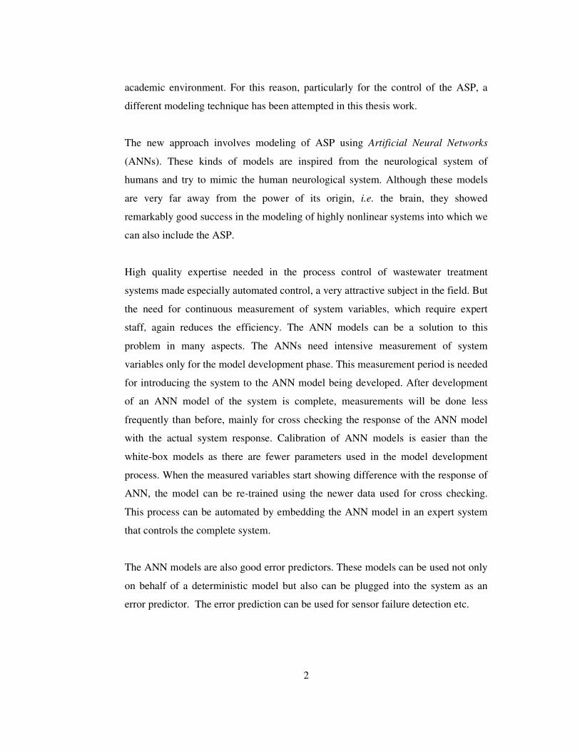
Figure 2.1 Schematic presentation of completely-mixed reactor with biomass
recycle and wasting: (a) from the reactor and (b) from the recycle line (Q: flow rate,
S: substrate concentration, X: biomass concentration; subscripts r: return, w: waste,
0: influent, e: effluent e.g. Qr: return flow rate) (Tchobanoglous and Burton, 1991). 5
Figure 2.2 A Biological Neuron.............................................................................10
Figure 2.4 An example of a recurrent network with self loops. ..............................14
Figure 2.5 Typical backpropagation feed-forward neural network. ........................15
Figure 2.6 Graphs of the typical transfer functions used in ANN models, (a)
logarithmic sigmoid function, (b) hyperbolic tangent function,.(c) linear function
(Matlab Help, 2002). .............................................................................................17
Figure 3.2 Main Graphical User Interface of NNTOOL Toolbox...........................33
Figure 3.3 Second GUI of NNTOOL Toolbox.......................................................33
Figure 3.1 General Layout of Ankara Central Wastewater Treatment Plant. ..........39
Figure 4.1 MLVSS output of the SSSP simulation.................................................45
Figure 4.2 Xhet output of the SSSP simulation........................................................46
Figure 4.3 Ss output of the SSSP simulation program. ...........................................46
Figure 4.4 Schematic view of ANN Model developed for SSSP. ...........................49
Figure 4.5 The ANN Model run results for MLVSS predictions Trials 1 to 3.........50
Figure 4.6 ANN Model run results for MLVSS predictions Trials 4 and 5. ............50
Figure 4.7 Regression analysis result of MLVSS variable for Trial5 ANN model. .51
Figure 4.8 Results obtained in the 1st run with the script: trainbr with number of
HNs: 3...................................................................................................................53
Figure 4.9 Results of the 1st run with the script: trainlm with number of HN: 9.....54
Figure 4.10 The results of the 2nd run with the script; using traincgp with four
number of HN .......................................................................................................55
Figure 4.11 The results of the 2nd run with the script; using traingda with ten
number of HN .......................................................................................................57

xiv
Figure 4.12 Sensitivity test results of MLVSS for SSSP Hypothetical WWTP for
changed Qinf. .........................................................................................................60
Figure 4.13 Sensitivity results of MLVSS for changed Qinf in ANN Model ...........61
Figure 4.14 Sensitivity results of Xhet for SSSP Hyp.WWTP for changed Qinf. ......61
Figure 4.15 Sensitivity results of Xhet for changed Qinf in ANN Model. .................62
Figure 4.16 Sensitivity results of Ss for SSSP Hyp. WWTP for changed Qinf. ........62
Figure 4.17 Sensitivity results of Ss for changed Qinf in ANN Model .....................63
Figure 4.18 Sensitivity test results of MLVSS for SSSP Hyp.WWTP for changing
Qinf. .......................................................................................................................63
Figure 4.19 Sensitivity results of MLVSS for changed Qinf in ANN Model ...........64
Figure 4.20 Sensitivity results of Xhet for SSSP Hyp. WWTP for changed Xi. .......64
Figure 4.21 Sensitivity results of Xhet for changed Xi in ANN Model ....................65
Figure 4.22 Sensitivity results of Ss for SSSP Hyp. WWTP for changed Xi. ..........65
Figure 4.23 Sensitivity results of Ss for changed Xi in ANN Model .......................66
Figure 4.25 Regression analysis of the best ANN model........................................72
Figure 4.26 Prediction of COD in the best ANN model with R=0.795 ...................73
Figures 4.27 Best model developed (traincgb, 4 HNs) for ACWTP. ......................80
Figures 4.28 Regression analysis for the best model developed for ACWTP. ........80
Figures 4.29 training session for the best model developed for ACWTP................82
Figures 4.30 Prediction with poly. data using two hidden layers for ACWTP. .......83
Figure B.1 ANN Model run results for Xhet predictions for Trial5..........................95
Figure B.2 Regression analysis result of Xhet variable for Trial5 ANN model. .......95
Figure B.3 ANN Model run results for Ss predictions for Trial5. ...........................96
Figure B.4 Regression analysis result of Ss variable for Trial5 ANN model. .........96

xv
LIST OF ABBREVIATIONS
IskWTP : skenderun Wastewater Treatment Plant
ACWTP : Ankara Central Wastewater Treatment Plant
ASP : Activated Sludge Process
SSSP : Simulation of Single-Sludge Processes for Carbon Oxidation,
Nitrification and Denitrification
Q : flow rate.
Ss : Slowly biodegradable solids.
MLVSS : Mixed Liquor Volatile Suspended Solids
Xhet : Heterotrophic Biomass
Xs : Autotrophic Biomass
ANN : Artificial Neural Networks
WWTP : Wastewater Treatment Plant
SRT : Solid Retention Time
PCA : Principle Component Analysis
ASM : Activated Sludge Model
NNTOOL : Neural Network Toolbox (MATLAB Mathworks Inc.)
HRT : Hydraulic Retention Time
MR : Multiple Regression
DBP : Disinfection by-products
ARX : Autoregressive Model with External Inputs
RTC : Real Time Control
FAS : Fuzzy Adaptive Systems
BNR : Biological Nutrient Removal
RMSE : Root Mean Squared Error
TOC : Total Organic Carbon
IAWPRC : International Association on Water Pollution Research and Control

xvi
PAO : Phosphorus accumulating organisms
bio-P : Biological phosphorus removal
Combo. : Combination
Q1inf : influent flow rate of line 1.
CODinf : influent chemical oxygen demand
Alk. : alkalinity
Qret : return flow rate
Twater : temperature of water
Tair : temperature of air c : solids retention time
eff. : effluent
# : number

1
CHAPTER I
1. INTRODUCTION
1.1. General
Environmental preservation efforts and developments in the technology have
resulted in stringent discharge standards. For this reason, significant amount of
investment has gone continuously to wastewater treatment over the years.
Consequently the water infrastructures have now been equipped with substantial
hardware and software for optimal control and management to compensate for the
lack of expertise and staff in the field. Biological treatment systems are usually
located away from settlements and the personnel are under constant health threat.
Therefore, automation to minimize personnel contact with these systems using
expert systems, such as artificial intelligence techniques using neural networks, has
become a popular and a very attractive issue.
The new concept about the treatment systems involves efficient operation as well as
good design to reach the goals. It should be understood that only efficiently operated
plants can make a maximum out of a good design. Consequently, process control
has become an important issue as well as the quality of the design. For the control of
the system, some deterministic models, which can also be called as white-box
models, have been developed. Although these models give a good insight into the
mechanism, they require a lot of hard work before applying to a specific wastewater
treatment plant.
The most important of the deterministic models are ASM1, ASM2, ASM3, and
ASM2d for activated sludge process (ASP). Determination of the model parameters
normally need extensive laboratory and computer work which is often confined to
2
academic environment. For this reason, particularly for the control of the ASP, a
different modeling technique has been attempted in this thesis work.
The new approach involves modeling of ASP using Artificial Neural Networks
(ANNs). These kinds of models are inspired from the neurological system of
humans and try to mimic the human neurological system. Although these models
are very far away from the power of its origin, i.e. the brain, they showed
remarkably good success in the modeling of highly nonlinear systems into which we
can also include the ASP.
High quality expertise needed in the process control of wastewater treatment
systems made especially automated control, a very attractive subject in the field. But
the need for continuous measurement of system variables, which require expert
staff, again reduces the efficiency. The ANN models can be a solution to this
problem in many aspects. The ANNs need intensive measurement of system
variables only for the model development phase. This measurement period is needed
for introducing the system to the ANN model being developed. After development
of an ANN model of the system is complete, measurements will be done less
frequently than before, mainly for cross checking the response of the ANN model
with the actual system response. Calibration of ANN models is easier than the
white-box models as there are fewer parameters used in the model development
process. When the measured variables start showing difference with the response of
ANN, the model can be re-trained using the newer data used for cross checking.
This process can be automated by embedding the ANN model in an expert system
that controls the complete system.
The ANN models are also good error predictors. These models can be used not only
on behalf of a deterministic model but also can be plugged into the system as an
error predictor. The error prediction can be used for sensor failure detection etc.

3
In this study, firstly a hypothetical wastewater treatment plant was constructed with
the help of an ASM1 model simulator, SSSP program. The SSSP Program was used
as a hypothetical treatment plant, and then this hypothetical plant was modeled
using ANNs. After development of an ANN model using the SSSP default dynamic
input-output pattern, sensitivity analyses were carried out on both models using the
same data. Then two actual wastewater treatment plants were modeled. These
treatment plants were skenderun Wastewater Treatment Plant (IskWTP) and
Ankara Central Wastewater Treatment Plant (ACWTP). Approximately five months
of daily data for IskWTP and one year of daily data for ACWTP was used in the
modeling processes.
The ultimate aim of this thesis is therefore to develop an ANN model that is capable
of predicting outputs from ASP with high fidelity to the actual system; hence
somehow model the plant under consideration. To achieve this, various operational
parameters will be used as input to predict some of the selected output parameters
(influent/effluent chemical oxygen demand etc). In choosing the input parameters,
their demonstrated relationships to the output parameters and the biological
mechanism were taken into consideration. In addition to that, some combinations of
parameters that can be measured on-line continuously will be used to develop the
ANN model for precise operation of the system.

4
CHAPTER II
2. THEORETICAL BACKGROUND
2.1. Activated Sludge Process
The major biological processes used for wastewater treatment are aerobic, anoxic,
anaerobic processes, combined aerobic, anoxic and anaerobic processes and pond
processes. The individual processes are further subdivided, depending on whether
treatment is accomplished in suspended-growth systems or attached-growth systems
or combinations thereof (Tchobanoglous and Burton, 1991).
The activated sludge process, which is an aerobic suspended-growth treatment
system, was developed in England by Ardern and Lockett (1914) and was so named
because it involved the production of an activated mass of microorganisms capable
of stabilizing a waste aerobically. Many versions of the original process are in use
today, but fundamentally they are all similar (Tchobanoglous and Burton, 1991).
2.1.1. Process Description
Biological wastewater treatment with the ASP is typically accomplished using a
flow diagram as shown in Figure 2.1. Organic waste is introduced into a reactor
where an aerobic bacterial culture is maintained in suspension. The reactor contents
are referred to as the “mixed liquor”. In the reactor, the bacterial culture carries out
the conversion of organic pollutants in accordance with the stoichiometry shown in
Equations 2.1 and 2.2 (Tchobanoglous and Burton, 1991).
5
Figure 2.1 Schematic presentation of completely-mixed reactor with biomass
recycle and wasting: (a) from the reactor and (b) from the recycle line (Q: flow rate,
S: substrate concentration, X: biomass concentration; subscripts r: return, w: waste,
0: influent, e: effluent e.g. Qr: return flow rate) (Tchobanoglous and Burton, 1991).
Oxidation and synthesis:
)1.2(.275322 prodendotherNOHCNHCOnutrientsOCOHNS bacteria +++ →++
Endogenous respiration:
energyNHOHCOONOHC bacteria +++ →+ 3222275 255 (2.2)
COHNS is waste to be treated,

6
C5H7NO2 is the produced new bacterial cells.
The aerobic environment in the reactor is achieved by the use of diffused or
mechanical aeration, which also serves to maintain the mixed liquor in a completely
mixed regime. After a specified period of time, the mixture of old and new cells are
passed into a settling tank, where these cells are separated from the treated
wastewater. A portion of the settled cells is recycled to the aeration basin to
maintain the desired concentration of organisms in the reactor, and a portion is
wasted (Figure 2.1). The portion wasted corresponds to the newly grown cells. The
level at which the biological mass in the reactor should be kept depends on the
desired treatment efficiency and the efficacy of the aeration system (Tchobanoglous
and Burton, 1991).
2.1.2. Process analysis
In the system, reactor is mixed completely via diffused or mechanical aeration used
for both mixing and air supply. It is assumed that the concentration of the
microorganism in the effluent is negligible. As shown in Figure 2.1 (b), the settling
tank serves as an integral part of the activated sludge process. Therefore, for further
introduction of the mass balance and also for the development of the kinetic model
for the activated sludge process the following assumptions are accepted
(Tchobanoglous and Burton, 1991):
• waste stabilization is carried out by the microorganisms occurs in the aerator
unit,
• the volume used in the calculation of the mean cell residence time for the
system includes only the volume of the aerator unit.
The mean hydraulic retention time, HRT, for the reactor is defined as:
QV
HRT r= (2.3)

7
where; Vr = volume of the reactor, (L3)
Q = influent flow rate, (L3/T)
For the system shown in Figure 2.1(b), the mean cell residence time c is defined as
the mass of microorganisms in the reactor over the mass of microorganisms
removed plus microorganisms wasted from the system per day, and it is given by:
eerw
rc XQXQ
XV+
=θ (2.4)
where;
Qw = flow rate of liquid containing the biological solids to be wasted from
the system, (L3/T),
Qe = flow rate of the effluent, (L3/T),
Xe = effluent microorganism concentration, (M/L3).
Xr = microorganism concentration in return line, (M/L3).
The mass balance for the biomass in the entire system represented in Figure 2.1(b)
can be written as follows (Tchobanoglous and Burton, 1991):
)()( '0 greewr rVXQXQQXV
dtdX ++−= (2.5)
where rg’ is the net growth rate of microorganisms within the system.
Assuming that cell concentration in the effluent is zero and steady state condition
prevails i.e. dX/dt=0 and rearranging Eq. 2.5 gives:
dc
kYq −=θ1
(2.6)
where; Y = yield coefficient, (M/M),
q = specific substrate utilization rate, (1/T),
kd = decay coefficient, (1/T).

8
The mass balance around activated sludge process configuration shown in Figure
2.1(b) regarding substrate can be written as follows (Tchobanoglous and Burton,
1991):
)( '0 srr rVQSQSV
dtdS +−= (2.7)
2.2. Deterministic Models (ASM1, ASM2, ASM2d, ASM3)
The Activated Sludge Model No. 1 (ASM1; Henze et al., 1987) can be considered
as the reference model, since it initiated the general acceptance of WWTP models in
research and industry. This evolution was undoubtedly supported by the availability
of more powerful computers. Even today, the ASM1 model is in many cases still the
state of the art for modeling activated sludge systems (Gernaey et al., 2004).
ASM1 was primarily developed for municipal activated sludge WWTPs to describe
the removal of organic carbon compounds and N, with simultaneous consumption of
oxygen and nitrate as electron acceptors. The model furthermore aims at yielding a
good description of the sludge production. Chemical oxygen demand (COD) was
selected as the measure of the concentration of organic matter present. In the model,
the wide variety of organic carbon compounds and nitrogenous compounds are
subdivided into a limited number of fractions based on biodegradability and
solubility considerations (Gernaey et al., 2004).
The ASM3 model was also developed for biological N removal in WWTPs, with
basically the same goals as ASM1. The ASM3 model is intended to become the new
standard model, correcting for a number of defects that have appeared during the
usage of the ASM1 model (Gujer et al., 1999).
Models including biological phosphorus removal (bio-P) were first introduced by
the ASM2 model (Henze et al., 1995), which extends the capabilities of ASM1 to
describe bio-P removal. Chemical P removal via precipitation was also included in
9
the ASM2. Yet the model does not completely describe the bio-P processes
(Gernaey et al., 2004).
All these models are common in that they need expertise to be calibrated for specific
treatment systems that they are tried to be applied. Parameter estimation of the
models is very hard in all the deterministic models. In contrast to this, data driven
models such as ANN does not need that much expertise. As a result, latter models
received attention from the academia as well as the industry.
2.3. Artificial Neural Networks
Hecht-Nielsen defined a neural network as: “… a computing system made up of a
number of simple highly interconnected processing elements, which processes
information by its dynamic state response to external inputs” (Chitra, 1993).
Neural network technology came from current studies of mammalian brains,
particularly the cerebral cortex. Neural networks mimic the way that a human brain
copes with incomplete and confusing information set (Chitra, 1993). In general, the
human nervous system is a very complex neural network. The brain is the central
element of the human nervous system, consisting of nearly 1010 biological neurons
that are connected to each other through sub-networks.
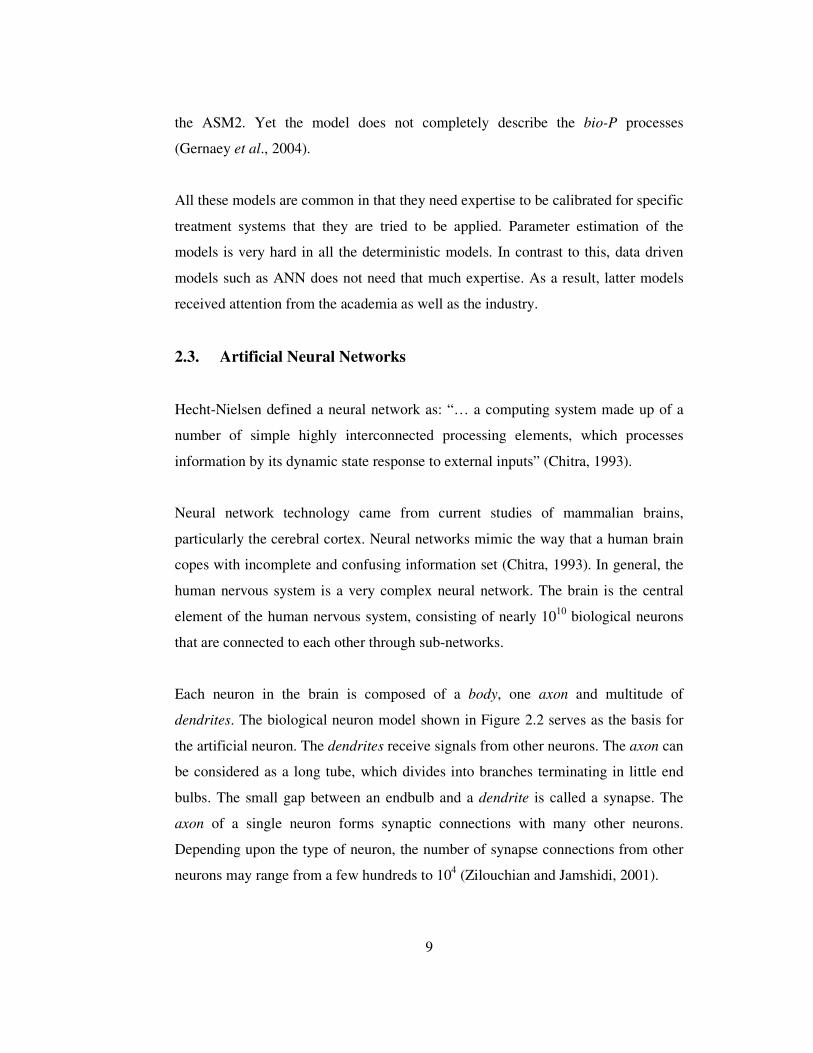
Each neuron in the brain is composed of a body, one axon and multitude of
dendrites. The biological neuron model shown in Figure 2.2 serves as the basis for
the artificial neuron. The dendrites receive signals from other neurons. The axon can
be considered as a long tube, which divides into branches terminating in little end
bulbs. The small gap between an endbulb and a dendrite is called a synapse. The
axon of a single neuron forms synaptic connections with many other neurons.
Depending upon the type of neuron, the number of synapse connections from other
neurons may range from a few hundreds to 104 (Zilouchian and Jamshidi, 2001).

10
The ability to learn is a fundamental trait of intelligence. Although a precise
definition of learning process is difficult to formulate, a learning process in ANN
context can be viewed as the problem of updating network architecture and
connection weights so that a network can efficiently perform a task. The network
usually must learn the connection weights from available training patterns and these
patterns should be representative of the system to be modeled (Jane et al, 1996).
Figure 2.2 A Biological Neuron.
Instead of executing a series of instructions, like an ordinary computer, a neural
network responds – in parallel – to the inputs given to it. The final result consists of
an overall state of the network after it has reached a steady-state condition, which
correlates patterns between the sets of input data and corresponding output or target
values. The final network can be used to predict outcomes from new input data
(Chitra, 1993).
Neural networks can learn complex nonlinear relationships even when the input
information is noisy and imprecise. Neural networks have made strong advances in
the areas of continuous speech recognition, pattern recognition, and classification of
noisy data, nonlinear feature detection, market forecasting, and process control and
modeling.

11
For example, consider how a child learns to identify shapes and colors using a toy
consisting of different solid shapes (triangles, squares, circles, and so on) and colors
that can be inserted into a box only through correspondingly shaped holes and
colors. The child learns about shapes and colors by repeatedly trying to fit the solid
objects through these holes by trial-and-error attempts. Eventually, the shapes and
colors are recognized, and the child is able to match the objects with the holes by
visual inspection. Similarly, neural networks learn by repeatedly trying to match the
sets of input data to the corresponding output target values. After a sufficient
number of learning iterations, the network creates an internal model that can be used
to predict for new input conditions (Chitra, 1993).
An artificial neural network is an information-processing system that has certain
performance characteristics in common with biological neural networks. ANNs
have been developed as generalizations of mathematical models of human cognition
or neural biology, based on the assumptions that:
1. Information processing occurs at many simple elements called neurons.
2. Signals are passed between neurons over connection links.
3. Each connection link has an associated weight, which, in a typical neural
net, multiplies the signal transmitted.
4. Each neuron applies an activation function (usually nonlinear) to its net
input (sum of weighted input signals) to determine its output signal.
A neural network is characterized by (1) its pattern of connections between the
neurons (called its architecture), (2) its method of determining the weights on the
connections (called its training or learning algorithm), and (3) its activation
function.
A neural network consists of a large number of simple processing elements called
neurons (units, cells, or nodes). Each neuron is connected to other neurons by means
12
of directed communication links, each with an associated weight. The weights
represent information being used by the network to solve a problem.
Each neuron has an internal state, called its activation or activity level, which is a
function of the inputs it has received. Typically, a neuron sends its activation as a
signal to several other neurons. It is important to note that a neuron can send only
one signal at a time, although that signal is broadcast to several other neurons
(Fausett, 1994).
2.3.1. Application Areas of ANNs
The study of neural networks is an extremely interdisciplinary field, both in its
development and in its application. The examples of applications of ANNs range
from commercial successes to areas of active research that show promise for the
future (Jain and Mao, 1996).
In signal processing, ANNs were used commercially in suppressing the noise on a
telephone line. In pattern classification, ANNs are used in character recognition,
speech recognition, EEG waveform classification, blood cell classification, and
printed circuit board inspection. In optimization, ANNs are used in a wide variety of
fields such as mathematics, statistics, engineering, science, and medicine. In control,
ANNs are used in control of dynamic systems (Jain and Mao, 1996).
2.3.2. Types of ANNs
ANNs are commonly classified by their network topology, node characteristics,
learning, or training algorithms (Fausett, 1994). Based on the connection pattern
(architecture), ANNs can be grouped into two categories (Figure 2.3- taxonomy of
neural network architectures) (Jane et al, 1996):
• Feed-forward networks, in which network have no looped connections and

13
• Feedback (recurrent) networks, in which loops occur because of feedback
connections.
In the most common family of feed-forward networks, called multilayer perceptron,
neurons are organized into layers that have unidirectional connections between
them. Different connection patterns yield different network behaviors. Generally
speaking, feed-forward networks are static, that is, they produce only one set of
output values rather than a sequence of values from a given input. Different network
architectures require appropriate learning algorithms (Jane et al, 1996). A feed-
forward network with one hidden layer of neurons is given in Figure 2.3.
Figure 2.3 Taxonomy of feed-forward and recurrent/feedback neural network
architectures.
In a feed-forward neural network structure, the only appropriate connections are
between the outputs of each layer and the inputs of the next layer. In this topology,
the inputs of each neuron are the weighted sum of the outputs from the previous
layer. If the weight of a branch is assigned a zero, it is equivalent to no connection
between corresponding nodes (Konar, 1999).
14
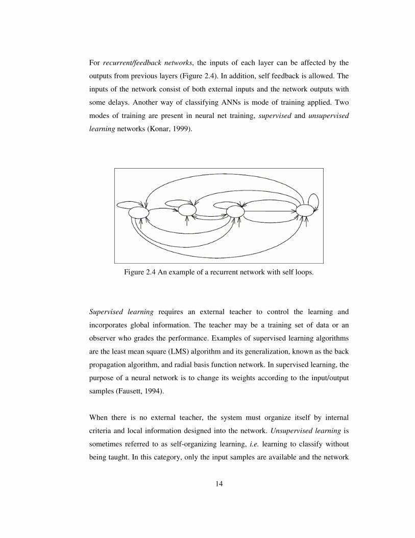
For recurrent/feedback networks, the inputs of each layer can be affected by the
outputs from previous layers (Figure 2.4). In addition, self feedback is allowed. The
inputs of the network consist of both external inputs and the network outputs with
some delays. Another way of classifying ANNs is mode of training applied. Two
modes of training are present in neural net training, supervised and unsupervised
learning networks (Konar, 1999).
Figure 2.4 An example of a recurrent network with self loops.
Supervised learning requires an external teacher to control the learning and
incorporates global information. The teacher may be a training set of data or an
observer who grades the performance. Examples of supervised learning algorithms
are the least mean square (LMS) algorithm and its generalization, known as the back
propagation algorithm, and radial basis function network. In supervised learning, the
purpose of a neural network is to change its weights according to the input/output
samples (Fausett, 1994).
When there is no external teacher, the system must organize itself by internal
criteria and local information designed into the network. Unsupervised learning is
sometimes referred to as self-organizing learning, i.e. learning to classify without
being taught. In this category, only the input samples are available and the network
15
classifies the input patterns into different groups. Kohonen network is an example of
unsupervised learning (Konar, 1999).
2.3.3. Typical Feed-forward Backpropagation ANN working
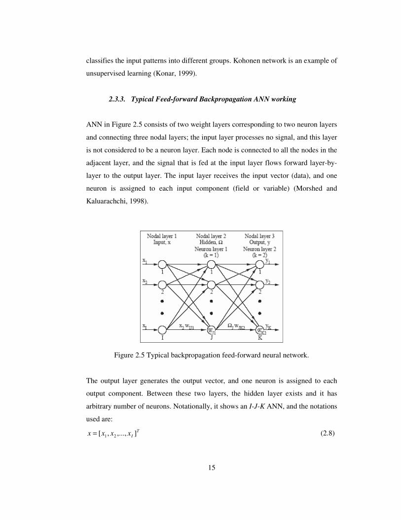
ANN in Figure 2.5 consists of two weight layers corresponding to two neuron layers
and connecting three nodal layers; the input layer processes no signal, and this layer
is not considered to be a neuron layer. Each node is connected to all the nodes in the
adjacent layer, and the signal that is fed at the input layer flows forward layer-by-
layer to the output layer. The input layer receives the input vector (data), and one
neuron is assigned to each input component (field or variable) (Morshed and
Kaluarachchi, 1998).
Figure 2.5 Typical backpropagation feed-forward neural network.
The output layer generates the output vector, and one neuron is assigned to each
output component. Between these two layers, the hidden layer exists and it has
arbitrary number of neurons. Notationally, it shows an I-J-K ANN, and the notations
used are: T
Ixxxx ],...,,[ 21= (2.8)
16
TJ ],...,,[ 21 ΩΩΩ=Ω (2.9)
TKyyyy ],...,,[ 21= (2.10)
TKJjk wwwww ],...,,...,,[ 21 += (2.11)
TKJjk wwwww ],...,,...,,[ 21 += (2.12)
where x = input vector of I components; Ω = hidden vector of J components; y =
ANN output vector of K components; w = threshold weight vector of (J + K)
components where JKw = threshold of jth neuron in (k+1)th neuron layer; and w =
weight vector of J(I + K) components where wijk is the weight connecting ith neuron
in kth neuron layer to jth neuron in (k+1)th layer. ANN may be noted to have
)()( KIJKJM +++= M weights where M is the total number of weights. Hecht-
Nielsen’s suggestion (1987) is used to define an upper limit of J = (2I + 1) neurons
in the hidden layer. Finally, each hidden or output neuron is associated with a
transfer function, f(·) (Morshed and Kaluarachchi, 1998).
In simulating the x–y response for a given x, ANN follows two steps. First, x is fed
at the input layer, and ANN generates Ω as
11
=
+=Ω
=kxwwf
I
iiijkjkj (2.13)
Second, ANN presents Ω to the output layer to generate y as
21
=
Ω+= =
kwwfyJ
iiijkjkj (2.14)
Equation 2.15 is the ANN response y to x, and y may be expressed as
( )xwwy jj ,,Γ= (2.15)
[ ]TK )(),...,(),()( 21 ⋅Γ⋅Γ⋅Γ=⋅Γ (2.16)
where; )(⋅Γ = underlying x-y response vector approximated by ANN;
)(⋅Γ j =jth component of )(⋅Γ .
Thus, ANN may be viewed to follow the belief that intelligence manifest itself from
the communication of a large number of simple processing elements. The transfer
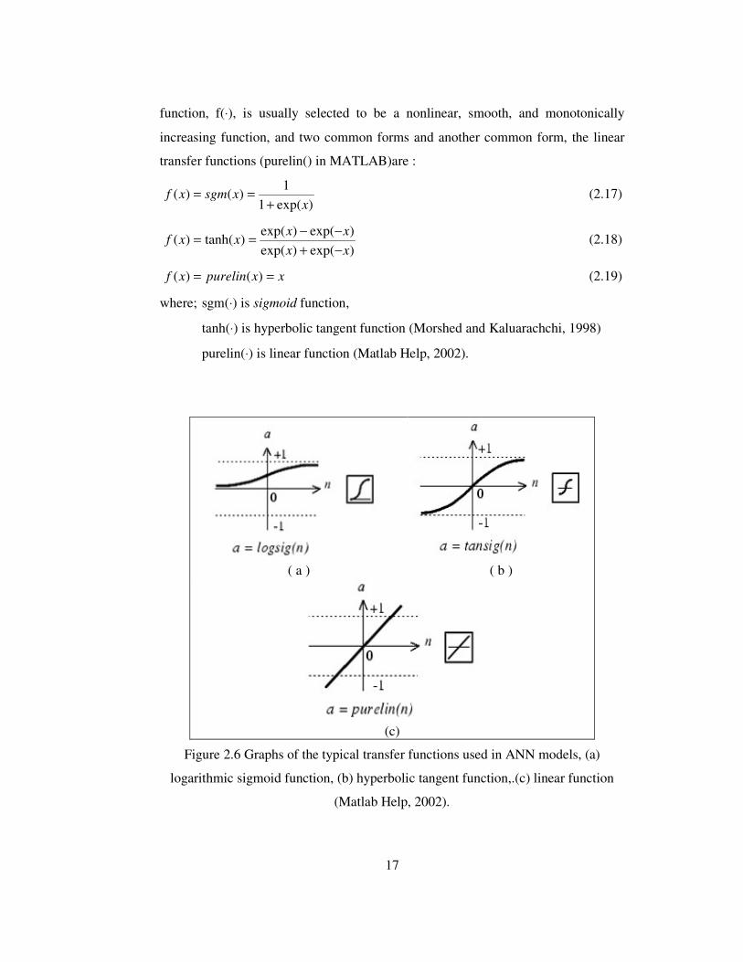
17
function, f(⋅), is usually selected to be a nonlinear, smooth, and monotonically
increasing function, and two common forms and another common form, the linear
transfer functions (purelin() in MATLAB)are :
)exp(11
)()(x
xsgmxf+
== (2.17)
)exp()exp()exp()exp(
)tanh()(xxxx
xxf−+−−== (2.18)
xxpurelinxf == )()( (2.19)
where; sgm(⋅) is sigmoid function,
tanh(⋅) is hyperbolic tangent function (Morshed and Kaluarachchi, 1998)
purelin(⋅) is linear function (Matlab Help, 2002).
( a )
( b )
(c)
Figure 2.6 Graphs of the typical transfer functions used in ANN models, (a)
logarithmic sigmoid function, (b) hyperbolic tangent function,.(c) linear function
(Matlab Help, 2002).
18
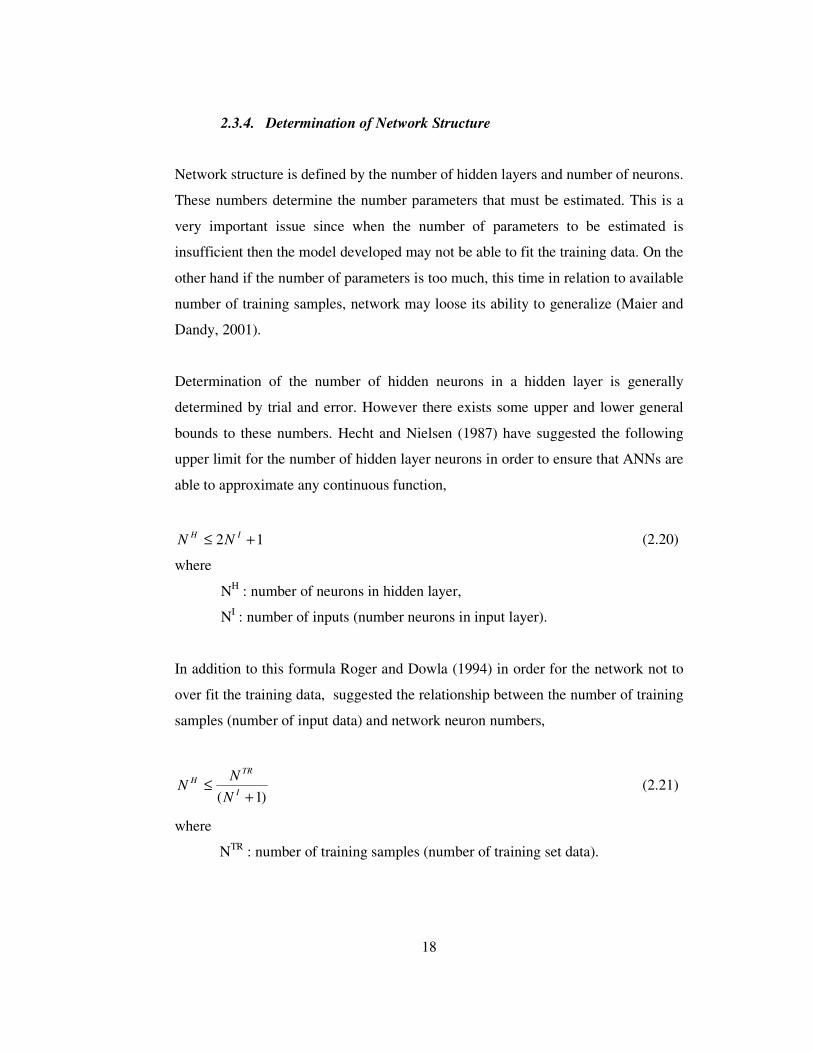
2.3.4. Determination of Network Structure
Network structure is defined by the number of hidden layers and number of neurons.
These numbers determine the number parameters that must be estimated. This is a
very important issue since when the number of parameters to be estimated is
insufficient then the model developed may not be able to fit the training data. On the
other hand if the number of parameters is too much, this time in relation to available
number of training samples, network may loose its ability to generalize (Maier and
Dandy, 2001).
Determination of the number of hidden neurons in a hidden layer is generally
determined by trial and error. However there exists some upper and lower general
bounds to these numbers. Hecht and Nielsen (1987) have suggested the following
upper limit for the number of hidden layer neurons in order to ensure that ANNs are
able to approximate any continuous function,
12 +≤ IH NN (2.20)
where
NH : number of neurons in hidden layer,
NI : number of inputs (number neurons in input layer).
In addition to this formula Roger and Dowla (1994) in order for the network not to
over fit the training data, suggested the relationship between the number of training
samples (number of input data) and network neuron numbers,
)1( +≤
I
TRH
NN
N (2.21)
where
NTR : number of training samples (number of training set data).
19
2.4. Literature Survey
2.4.1. Uses of Artificial Neural Networks in Ecological Sciences
Most applications of ANNs in biology have been in medicine and molecular biology
(Lerner et al., 1994; Albiol et al., 1995; Faraggi and Simon, 1995; Lo et al., 1995).
At the beginning of the 90’s a few applications of this method were reported in
ecological and environmental sciences. For instance, Colasanti (1991) found
similarities between ANNs and ecosystems and recommended the utilization of this
tool in ecological modeling. In a review by Edwards and Morse (1995) on
computer-aided research in biodiversity, important potential of ANNs have been
underlined.
Relevant examples are found in very different fields in applied ecology, such as
modeling the greenhouse effect (Seginer et al., 1994), predicting various parameters
in brown trout management (Baran et al., 1996; Lek et al., 1996a,b), modeling
spatial dynamics of fish (Giske et al., 1998), predicting phytoplankton production
(Scardi, 1996; Recknagel et al., 1997), predicting fish diversity (Guégan et al.,
1998), predicting production: biomass (P:B) ratio of animal populations (Brey et al.,
1996), predicting farmer risk preferences (Kastens and Featherstone, 1996), etc.
Most of these works showed that ANNs performed better than the more classical
modeling methods (Lek and Guégan, 1999).
In a study by Lek et al. the predictive capacity of multiple regression (MR) versus
artificial neural network (ANN) for the estimation of brown trout redds from
physical habitat variables in six mountain streams in SW France are compared.
Model-predicted and observed values are compared by different statistical
parameters, normality and correlation of the residuals. To compare the models (MR
and ANN), authors worked with transformed (requirement of MR) and non-
transformed (raw data) variables. Three indicators to judge the quality of the results
obtained in the MR and ANN are used.

20
The correlation coefficient R between observed and estimated values, or the
determination coefficient R2; the slope of the regression between values estimated
by models and observed values; and the study of residuals iii YYE ˆ−= , their
statistical parameters, graphs of normality. The MR model is shown to have
difficulty in predicting the low and high values in the data set. Also a negative value
prediction is shown by MR model, especially for the low values. For ANN, this
problem remains with the transformed values, however with non-transformed
variables; an excellent model was obtained capable of restoring values observed
over the whole range of the dependent variable. Also ANN model unlike MR model
never predicted negative values.
This study showed that MR or ANN can be used to predict the density of brown
trout redds from the sampled physical habitat variables, R2 reached 0.65 in MR and
R2 reached 0.96 in ANN; which gave the better result with the non-transformed
variables.
The ANNs constitute a new and alternative approach in ecology. They are able to
work with nonlinearly related variables. As a matter of fact they do not set
constraints on the variables (e.g. normality and/or nonlinear relationships), better
still, they can be more efficient working with raw than with transformed data.
Unlike MR, ANN provides simple equations for users but it is possible to easily
quantify the contribution of each variable over its range from the weight distribution
in the model ANN. It can be concluded that the ANN models can successfully be
used in ecological modeling, especially for predictive modeling and ANNs showed
better results than the traditionally used models in ecological modeling (Lek et al.,
1996).

21
2.4.2. Uses of ANNs in Environmental Sciences
The ability of two empirical modeling approaches to forecast residual chlorine
evolution in two drinking water systems were evaluated (Rodriguez and Sérodes,
1999). The purpose was to compare the forecasting capabilities of a linear model,
known as linear autoregressive model, with external inputs (ARX) and a non-linear
model (ANNs). The assessment of the benefits in using non-linear models when
simulating the decay of residual chlorine in water systems is discussed.
Two case studies were used to compare accuracy of the two kinds of models (ARX
vs. ANN). Data from two Quebec (Canada) drinking water systems were used in the
study. The first system (denoted as case 1) was a storage tank located within the
distribution system of the city of Sainte-Foy. The second system (denoted as case 2)
was the main water pipeline of the city of Quebec’s distribution system. For both
cases, the linear (ARX) and non-linear (ANN) modeling approaches were used to
forecast concentrations of residual chlorine at monitored points located downstream
from the dose application point (Rodriguez and Sérodes, 1999). Modeling process
started from a less complicated structure towards more complicated resulting
progressively in higher accuracy.
Another study on water systems was on the real time control of such systems by H.
Lobbrecht and Solomatine (2002). Aim of the study was to real time control (RTC)
the combined urban and rural water systems. The so-called centralized control
requires information from different locations in the water system and hence is
sensitive to the communication network breakdown during extreme storm runoff
events. To overcome these problems, the application of machine learning methods
was proposed, using artificial neural networks and fuzzy adaptive systems (FAS).
The intelligent controllers developed are appeared to be robust and capable of
solving RTC problems on the basis of information measured only locally.
Computing times were reduced by two orders of magnitude by using local

22
intelligent controller replicates of central control behavior. This makes the machine-
learning techniques (ANN and FAS) useful for application in real-life situations of
water management (Lobbrecht and Solomatine, 2002).
A software sensor design based on empirical data obtained from a physical sensor
which is responsible for the measurement of ammonia in rivers and wastewater
treatment plants was developed by M. H. Masson (1999). The aim of the study was
to have a software sensor that was capable of determining the ammonia levels in the
field of interest quicker than the physical one that results the measurement in 20 –
25 min. This would allow the control measures to be taken earlier.
In the study of Murtagh et al. (2000), a neural network model in the environment
and climate Neurosat (“Processing of Environmental Observing Satellite Data with
Neural Networks”) project was tried for the prediction of oceanic upwelling of the
Mauritanian coast, using sea surface temperature (SST) images, and real and model
meteorological data for the year of 1982. The overall themes of the study were data
and information fusion. The empirical and model-based handling of data was
characterized by many uncertainties and numerous missing cases; and the
development of data-driven pattern recognition and neural network methods. It was
sought whether such methods are an alternative to, or are complementary to, large
physical simulation and modeling systems.
Studies on development of neural network based sensor systems for environmental
monitoring is done by Keller et al (1994). The study is comprised of development of
three prototype sensing systems that are composed of sensing elements, data
acquisition system, computer, and neural network implemented in software.
The first system employs an array of tin-oxide gas sensors and is used to identify the
composition of chemical vapors. The second system employs an array of optical
sensors and is used to identify the composition of chemical dyes in liquids. The
third system contains a portable gamma-ray spectrometer and is used to identify

23
radioactive isotopes. The aim is to develop compact, portable systems capable of
quickly identifying contaminants in the environment (Keller et al., 1994).
2.4.3. Previous Studies on modeling of Activated Sludge Plant using
Artificial Neural Networks
The activated sludge process, comprising a biological reactor and a secondary
settler, is widely used as secondary treatment for both municipal and industrial
wastewaters. The effective control of such a process depends, in part, on the ability
to simulate the dynamics of both the biological reactor and the secondary clarifier.
Considerable effort has therefore been devoted to the modeling of the activated
sludge process since the early 1970’s.
The advent of neural networks opens another door in the field of modeling and
control as they can be coupled with mechanistic models to increase the prediction
capabilities without necessarily increasing the mathematical complexities in the
mechanistic model. The objective of the authors is to report on the improvement of
an existing mechanistic model of the activated sludge process using a black box
model: ANNs (Côte et al., 1995).
A set of 193 hourly samples were used for the modeling of the ANN. The first 140
data were used for the training (learning) process (analogous to the parameter
estimation in the mechanistic model), and the remaining data served as a validation
file, on which generalizing capability of the network could then be judged.
Coupling of the mechanistic model with the neural network error predictor yielded
significant improvement in the simulation of all the variables. This is especially true
for the cases where the mathematical expressions of the mechanistic model were
insufficient in describing the complex phenomena occurring within the process, e.g.
suspended solids in the effluent.
24
Coupling of neural network error predictor is shown to result in beneficial
information about the mechanistic models. If outputs are predicted better by the use
of ANNs, which are data driven models, compared to mechanistic models this
implies that the mechanistic model can not capture everything underlying in the
system. This is a clear indication that the experimental data contains dynamic
behavior that has not been encapsulated in the mechanistic model and the ANN
modeling effort would lead to a better model (Côte et al., 1995).
A virtual software sensor for optimal control of a wastewater treatment process is
tried to be developed (Choi and Park, 2001) using artificial neural networks as a
modeling tool coupled with principle component analysis (PCA).
The influent wastewater quality data that were measured daily for 113 days at an
industrial wastewater treatment plant was used to derive the ANN model (software
sensor). Evaluation of the applicability of a hybrid neural network (PCA + ANN), as
a software sensor, was compared with four different methods including multivariate
regression, principal component regression, neural networks, and hybrid neural
networks. The Total Khjeldal Nitrogen (TKN) was selected as the object output
parameter that has to be estimated and 11 parameters were used as input variables.
In order to increase the sensitivity of the ANN model and enhance the prediction
capability, 11 wastewater parameters were reduced to 5 principle components (PCs),
which became the principle input parameters of the improved ANN model.
The study confirmed that in modeling of correlated noisy data, the preprocessing
using PCA to reduce the number of input variables was effective. Performance
criteria used in the study was RMSE (root mean squared error); which is reduced
from 66.50 in ANN to 13.82 in ANN + PCA for the test data (Choi and Park, 2001).
It was shown that an industrial treatment plant can be modeled using ANNs. In this
study seven neural networks are used to simulate the treatment plant, one network
25
for each reactor, and another for the prediction of effluent total organic carbon
(TOC) based on the conditions for the last reactors. ASP is selected as removal
process because of the purified terephtalic acid in the wastewater (Gontarski et al.,
2000).
The following variables were used in the training of backpropagation neural
networks in the wastewater treatment plant: (a) the inlet wastewater TOC in each
reactor; (b) the ratio of influent to recycled sludge flow; (c) concentration of
suspended solids (sludge) in the reactors; (d) concentration of dissolved oxygen in
the reactors; (e) average sludge residence time; and (f) parameters related to reaction
kinetics (Gontarski et al, 2000).
In the study two reactor results were given. The sensitivity analysis based on the
two reactors showed that the liquid flow rate and pH of the inlet stream were the
most important parameters controlling the plant, where all other data were within
the range of data supplied in the training process (Gontarski et al, 2000). It is
concluded that the use of neural networks can establish a better operating condition,
which has been defined by variables such as the splitting ratio of the inlet stream for
each reactor. Neural networks are seen to represent a possible aid to operations in
order to predict disturbances proactively and act to minimize output fluctuations by
making the control of the treatment plant more effective (Gontarski et al, 2000).
In a recent study for a major wastewater treatment plant with an average flow rate of
1 million m3/day, past data of the plant were used in building a neural network
model of the plant in the Greater Cairo district, Egypt. BOD (Biochemical Oxygen
Demand) and SS (Suspended Solids) in the effluent stream were tried to be
modeled. The observed values for 10 months were taken from the laboratory of the
treatment plant. Two ANN models for each variable were built and these models
have shown high efficiency. Although the efficiency was high enough the authors
emphasized the importance of the amount and accuracy of the data as follows: if
more data were collected, if the data were less noisy, and if additional parameters

26
were measured (e.g. pH, temperature, etc.), this would have resulted in an improved
predictive capability of the network. Nevertheless, the ANN is a tool that is worth
consideration in the prediction of WWTPs (Hamed et al, 2004).
Zeng et al have made a study on modeling a paper mill wastewater treatment plant
having coagulation as the main mechanism of removal. In the study the authors tried
to model the nonlinear relationship between the pollutant removal rates with the
chemicals used for the coagulation using a multi-layer back-propagationn neural
network. Gradient descent method was used in model training (namely parameter
estimation in the deterministic models) and the results obtained have shown an
encouraging accuracy that the model could be used in control and reasonable
forecasting was achieved (Zeng et al, 2004).
27
CHAPTER III
3. MATERIALS AND METHODS
3.1. Artificial Neural Networks
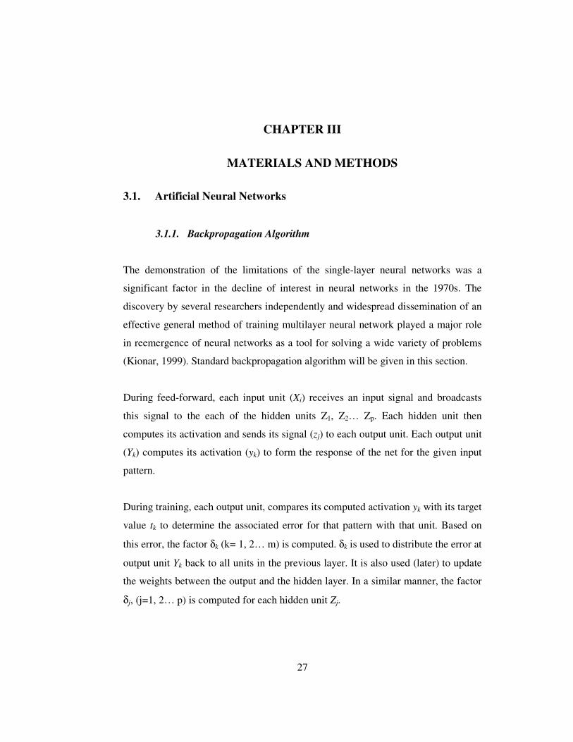
3.1.1. Backpropagation Algorithm
The demonstration of the limitations of the single-layer neural networks was a
significant factor in the decline of interest in neural networks in the 1970s. The
discovery by several researchers independently and widespread dissemination of an
effective general method of training multilayer neural network played a major role
in reemergence of neural networks as a tool for solving a wide variety of problems
(Kionar, 1999). Standard backpropagation algorithm will be given in this section.
During feed-forward, each input unit (Xi) receives an input signal and broadcasts
this signal to the each of the hidden units Z1, Z2… Zp. Each hidden unit then
computes its activation and sends its signal (zj) to each output unit. Each output unit
(Yk) computes its activation (yk) to form the response of the net for the given input
pattern.
During training, each output unit, compares its computed activation yk with its target
value tk to determine the associated error for that pattern with that unit. Based on
this error, the factor δk (k= 1, 2… m) is computed. δk is used to distribute the error at
output unit Yk back to all units in the previous layer. It is also used (later) to update
the weights between the output and the hidden layer. In a similar manner, the factor
δj, (j=1, 2… p) is computed for each hidden unit Zj.

28
After all the δ factors have been determined, the weights for all layers are adjusted
simultaneously. The adjustment to the weight wjk (from hidden unit Zj to output unit
Yk) is based on the factor δk and the activation zj, of the hidden unit Zj. The
adjustment to the weight vij (from input unit to Xi to hidden unit Zj) is based on the
factor δj and the activation xi of the input unit.
The algorithm can be written as follows:
Step 0: Weight initialization.
(set to small random values)
Step 1: While stopping criteria is false, do Steps 2-9.
Step 2: For each training pair, do Steps 3-8.
Feedforward:
Step 3: Each input unit (Xi, i =1, 2, …., n) receives input signal xi
and broadcasts this signal to all units in the layer above (the
hidden units).
Step 4. Each hidden unit (Zj, j =1, 2, …., p) sums its weighted input
signals, =
+=n
iijijj vxinz
10 ,_ ν applies its activation
function to compute its output signal, ),_( jj inzfz = and
sends this signal to all units in the layer above (output units).
Step 5. Each output unit (Yk, k =1, 2, …., m) sums its weighted input
signals, =
+=p
jjkjkk wzwiny
10 ,_ and applies its activation
function to compute its output signal, )_( kk inyfy = .
Backpropagation Error:
Step 6: Each output unit (Yk, k =1, 2, …., m) receives a target pattern
corresponding to the input training pattern, computes its error
information term, ),_()( kkkk inyfyt ′−=δ calculates its
weight correction term (used to update wjk later),
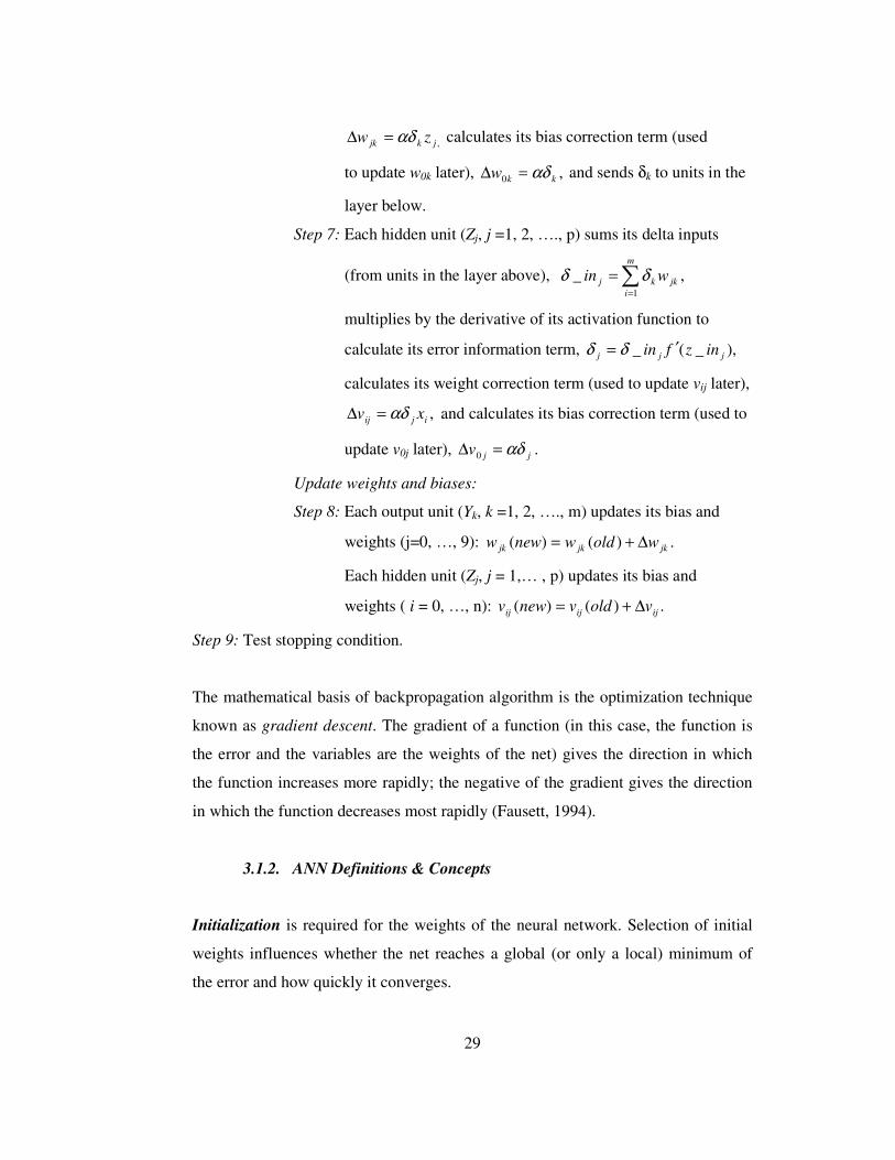
29
,jkjk zw αδ=∆ calculates its bias correction term (used
to update w0k later), ,0 kkw αδ=∆ and sends δk to units in the
layer below.
Step 7: Each hidden unit (Zj, j =1, 2, …., p) sums its delta inputs
(from units in the layer above), =
=m
ijkkj win
1
,_ δδ
multiplies by the derivative of its activation function to
calculate its error information term, ),_(_ jjj inzfin ′= δδ
calculates its weight correction term (used to update vij later),
,ijij xv αδ=∆ and calculates its bias correction term (used to
update v0j later), jjv αδ=∆ 0 .
Update weights and biases:
Step 8: Each output unit (Yk, k =1, 2, …., m) updates its bias and
weights (j=0, …, 9): .)()( jkjkjk woldwneww ∆+=
Each hidden unit (Zj, j = 1,… , p) updates its bias and
weights ( i = 0, …, n): .)()( ijijij voldvnewv ∆+=
Step 9: Test stopping condition.
The mathematical basis of backpropagation algorithm is the optimization technique
known as gradient descent. The gradient of a function (in this case, the function is
the error and the variables are the weights of the net) gives the direction in which
the function increases more rapidly; the negative of the gradient gives the direction
in which the function decreases most rapidly (Fausett, 1994).
3.1.2. ANN Definitions & Concepts
Initialization is required for the weights of the neural network. Selection of initial
weights influences whether the net reaches a global (or only a local) minimum of
the error and how quickly it converges.

30
An epoch is one cycle through the entire set of training vectors or predefined
number of points in the training vectors. Many epochs are required for training a
backpropagation neural net. A common variation is batch updating, in which weight
updates are accumulated over an entire epoch before being applied.
A relationship among the number of training patterns available, P, the number of
weights to be trained, W, and the accuracy of classification expected, e, is
summarized as: ePW = .
Data representation (normalization of data) in neural networks is also a very
important issue. In many problems, input vectors and output vectors have
components in the same range of values. In many neural network applications the
data may be given by either a continuous-valued variable or a “set or range”.
The aim of training a neural net is to have a balance between correct responses to
the training patterns and accurate responses to new input patterns. It is equivalent to
parameter estimation in traditional deterministic models. It is not always
advantageous to continue training until the total squared error reaches a minimum.
Hecht-Nielsen suggests using two distinct sets of data during training. One of these
sets is used for the weight adjustments, and the other one is used at some interval for
calculation of the error. If the error in the second test set continues to decrease,
training is continued. When the error in the test set (called validation set in
MATLAB NNTOOL Toolbox) starts increasing, the net starts memorizing the
training patterns. So the training session was stopped (Konar, 1999).
Stopping criteria can be defined as the criteria which result in stopping the training
session. Early stopping is important for improving generalization. In this technique
the available data is divided into three subsets. The first subset is the training set,
which is used for computing the error gradient and updating the network weights

31
and biases. The second subset is the validation set. The error on the validation set is
monitored during the training process. The validation error will normally decrease
during the initial phase of training, as does the training set error. However, when the
network begins to overfit the data, the error on the validation set will typically begin
to rise. When the validation error increases for a specified number of iterations
(called max fail in MATLAB Neural Network Toolbox), the training is stopped, and
the weights and biases at the minimum of the validation error are returned (Matlab
Help, 2002).
Network structure was defined before as the number of hidden neurons and hidden
layers. The limits on the number of hidden neurons and hidden layers defined by
Hecht and Nielsen (1987) and Rogers and Dowla (1994) were taken into
consideration in this study. Especially in ANN models with one hidden layer, the
upper of these limits were taken and were tried in the script. There were some space
and memory requirement problems in the ANN models with two hidden neurons
when running the script.
3.2. MATLAB Neural Network Toolbox (NNTOOL) & Scripting
3.2.1. Introduction to NNTOOL and Graphical User Interface
Model development was carried out by using MATLAB Package Program version
6.5 of Mathworks Company. MATLAB is a package program that consists of
toolboxes for various areas of engineering. NNTOOL – Neural Network Toolbox is
one of the toolboxes in MATLAB that implements ANNs and is used for the
modeling process. For an automated search in the solution space a script is written
that creates ANNs for a given training function, in a predefined range of hidden
layers, in a predefined range of number of neurons in the hidden layers, etc. The
details of script are given in the materials and methods section of the thesis.

32
MATLAB NNTOOL Toolbox is composed of two graphical user interface (GUI).
Network/Data Manager (Figure 3.2) deals with the communication between
MATLAB console and the NNTOOL, and creation and manipulation and addition
or subtraction of data or neural networks. Network (Figure 3.3) provides an
interface for initialization, training, simulation etc. of ANNs in the Network/Data
Manager.
The NNTOOL main GUI is given in Figure 3.2. GUI can be divided into two parts,
the data and network representations on top (Inputs, Outputs, Targets, Networks,
Errors, Input Delay States, and Layer Delay States). The data to be used can either
be exported from MATLAB console or from MATLAB data file (“.mat”).
Importing, exporting, deleting new data or new network, and creating new network
are done with corresponding buttons.
The second part of the GUI deals with network training, initialization etc as
mentioned before. This part implements the model building process. From the
second part of the main GUI the second GUI (Figure 3.3) that does initialization,
simulating, training, and adapting of neural networks that were either created or
exported to the main GUI.
The second GUI does everything on the neural network including showing the view
of neural network under consideration, training, initialization, simulation, adaptation
and showing the weights of the neural net.
NNTOOL was mainly used in this study to derive more accurate results from a pre-
developed neural net using the script written for automatic generation of ANN
models. NNTOOL is a very user friendly GUI that can be used in creation of small
number of models in specific problem domains.

33
Figure 3.2 Main Graphical User Interface of NNTOOL Toolbox.
Figure 3.3 Second GUI of NNTOOL Toolbox.
34
3.2.2. MATLAB Scripting
For the model development, a MATLAB script was written to automatically create
ANN models for IskWTP and ACWTP. The Script does the same thing that
NNTOOL GUI does. A graphical user interface (GUI) is shown in Figure 3.3. Script
was used to see the change in accuracy when various parameters of created neural
nets are changed.
The script has some different versions in which some main structures of the neural
nets were changed. For example one version of the script creates only neural nets
with only one hidden layer, and this script has three different versions in which
transfer functions were changed. The same thing has been applied to the one with
two hidden layers. The first version of the script is given in Appendix C.
The script mainly takes a data set from MATLAB workspace and then data is
normalized into either [0 1] or [-1 +1] range using “norm01.m” script written before
for [0 1], built-in premnmx function for [-1 +1] range. Then the script divides the
data into three subsets that will be used as training, validation and test set. The script
enters into a loop that creates neural nets for 13 of the MATLAB’s training
functions. These training functions are listed in Table 3.3.
For each of these training functions, the script enters into a second loop that changes
the number of hidden neurons in a predefined range. Before creating the next
network, the script trains the network and simulates the network with the given data
and makes a regression analysis of the results obtained at the beginning. After that
the next network is created and the same procedure above is applied. Also the script
saves the figures of the regression analysis of R (correlation coefficient) values
greater than some predefined threshold value, figure of observed versus predicted
COD, and figure of time series graph for observed versus predicted values of COD.

35
Table 3.3* training functions used to create ANN models using the script.
training function Brief Explanation
trainb Batch training with weight and bias learning rules. trainbfg BFGS quasi-Newton backpropagation. trainbr Bayesian regularization backpropagation
traincgb Conjugate gradient backpropagation with Powell-Beale restarts traincgf Conjugate gradient backpropagation with Fletcher-Reeves updates traincgp Conjugate gradient backpropagation with Polak-Ribiere updates traingd Gradient descent backpropagation traingda Gradient descent with adaptive learning rate backpropagation traingdm Gradient descent with momentum backpropagation
traingdx Gradient descent with momentum and adaptive learning rate backpropagation
trainlm Levenberg-Marquardt backpropagation trainoss One step secant backpropagation trainscg Scaled conjugate gradient backpropagation
3.3. SSSP - Simulation of Single-Sludge Processes for Carbon
Oxidation, Nitrification & Denitrification
SSSP is selected because it is a very powerful simulator for the activated sludge
process including the nitrification and denitrification. In addition, another reason for
the selection of the simulator is that it was used in many successful modeling studies
in the literature (Sin, 2000).
The SSSP system is an interactive, user-friendly program for simulating the
biological transformations occurring in the activated sludge of a wastewater
treatment plant performing simultaneous carbon oxidation, nitrification and
denitrification. Process rate expressions that model the biological transformations
were developed by a task group formed by IAWPRC. These rate expressions have
been incorporated into 12 material balances for the heterotrophic and autotrophic * Interested readers can refer to MATLAB Full Product Family Help R13 for more detailed
descriptions of these training algorithms.

36
biomass, soluble substrate, nitrate nitrogen, and other constituents that the task
considered significant in the process analysis of single-sludge wastewater treatment
plants. Utilizing numerical techniques, this program determines the solution to these
material balances for both constant and time dependent inputs.
The treatment plant is modeled as a chain of up to nine completely mixed reactors.
The user specifies the process flow scheme, basin volumes, the flow rate to each
reactor, the solids retention time (SRT), the kinetic parameters, the concentrations of
all components in the feed streams, and the time dependent pattern of all flow rates
and concentrations in those streams. Typical values of the kinetic parameters are
provided for simulation when complete kinetic data is unavailable. Interested
readers can refer to SSSP User’s Manual for the model assumptions, parameters,
and equations used. In this study the default dynamic example dataset is modeled.
Sensitivity analysis is applied on this dataset and the results obtained are given in
section results and discussion.
Dynamic solution menu in SSSP program is used to compute the solution to the
mass balance equations for input concentrations and flow rates that vary in
magnitude over a 24-hour cycle. To use the routine, variations in input (flow
pattern) must be supplied over a 24-hour cycle. SSSP program automatically
calculates the average flow rate and flow-weighted average concentrations and uses
them to compute the starting point for the numerical integration routine. Then the
computer repeats the integration over the 24-hour cycle until the variation in the
concentrations of the components is the same from one cycle to the next. In other
words, the computer determines the response of a system receiving the same 24-
hour input cycle day after day. Therefore, the system’s response depends only on
the daily variation in loading (Bidstrup and Grady, 1987).
The default dynamic example data set was supplied as input files, and they are
generated from typical settled American domestic wastewater constituent. This data
set is provided on the installation package for exploratory simulations into the
37
behavior of a system to “typical” input variations. The average flow rate on the
dynamic flow file is 1000 m3/d (Bidstrup and Grady, 1987). It was mentioned in the
SSSP manual that the set of dynamic data supplied was only for exploratory use. In
this study, the data was used only for that purpose. Although this data was not as
complex as the real world phenomena, this process was used as a practice in
understanding the ANN structure and concepts.
3.3.1. ANN Model development from SSSP Simulator Default Dataset
The default dynamic data set of SSSP was used in the modeling process. In this data
set, every parameter is given in a separate file. The input files have two columns, the
first column is the time and the second column is the corresponding value of the
parameter at that time. The extension of the input files is “.fed” and output file
extension for the dynamic output is “.dyn”. The default input files of the SSSP
program consists of 24 hour hourly data of the system variables used in the
calculations.
The SSSP Program has two types of data processing, e.i : “steady state solution” and
the “dynamic solution”, namely. The dynamic solution in SSSP is supplying 24 hour
input data using text file(s) therefore dynamic comes from this supplement.
Dynamic solution was used in this study. Three system variables were taken into
consideration in the model development process for the ANN model. The three
variables used are given in the Appendix A. These system variables are flow rate
(Q, m3/d), particulate products (Xi), autotrophic biomass (Xs, mg/l). The output
variables that were predicted by the model were mixed liquor volatile suspended
solids (MLVSS), heterotrophic biomass (Xhet, mg/l), and soluble organics (Ss).
Brief descriptions of the variables used in the modeling process are as follows:
Xhet: Heterotrophic biomass- Represents the biomass which uses readily
biodegradable substrate as both source of carbon for synthesis and source of energy

38
for maintaining life functions. It grows under aerobic and anoxic conditions, but not
under anaerobic conditions. Decay results in the conversion of biomass into slowly
biodegradable substrate and into particulate products which are not biodegradable.
Heterotrophs take up ammonia for cell synthesis under aerobic and anoxic
conditions, and convert nitrate nitrogen to gaseous N2 under anoxic conditions.
Xs: Autotrophic biomass – Represents the biomass which uses carbon dioxide as its
carbon source for synthesis, and converts ammonia into nitrate for energy. It grows
only under aerobic conditions. Decay results in the conversion of biomass into
slowly biodegradable substrate and particulate products which are not
biodegradable. Autotrophs also take up ammonia nitrogen for cell synthesis during
aerobic growth. This biomass includes both Nitrobacteria and Nitrosomonas
bacteria which are grouped together for the purposes of simulation.
Ss: Slowly biodegradable COD – Represents particulate and high molecular weight
organic material which is hydrolyzed extracellularly into readily biodegradable
COD. The rate of hydrolysis is lower than the rate of uptake of readily
biodegradable substrate.
3.4. Ankara Central Wastewater Treatment Plant
Ankara Central Wastewater Treatment Plant (ACWTP) has been constructed for a
capacity of 765000 m3/d wastewater to be treated by using activated sludge process.
The treatment plant was scheduled to serve for a population equivalent of six
million by year 2025. It has also been designed to include nitrogen and phosphorus
removal units in the future.
The plant employs activated sludge process with anaerobic sludge stabilization.
Sewerage system of the city was constructed in phase with the construction of the
wastewater treatment plant. When the sewerage system is completed, the 98% of the
city wastewater will have been collected to be treated by the plant.

39
3.4.1. Treatment Plant Layout & Dimensions
At the first stage of ACWTP, there are grid chambers, coarse and fine screens, as
the standard preliminary treatment units. These are followed by 10 primary
sedimentation tanks each with a diameter of 50 m. Primary sedimentation is
followed by 5 rectangular aeration tanks of 35m by 153 m. For the final
clarification, 20 secondary sedimentation tanks exist each having a 55 m diameter.
A battery of 90 surface aerators supplies air to biological reactions. Effluent COD
achieved is less than 30 mg/l for most of the time which is below the discharge
standards. General layout of the treatment plant is given in Figure 3.1.
Figure 3.1 General Layout of Ankara Central Wastewater Treatment Plant.
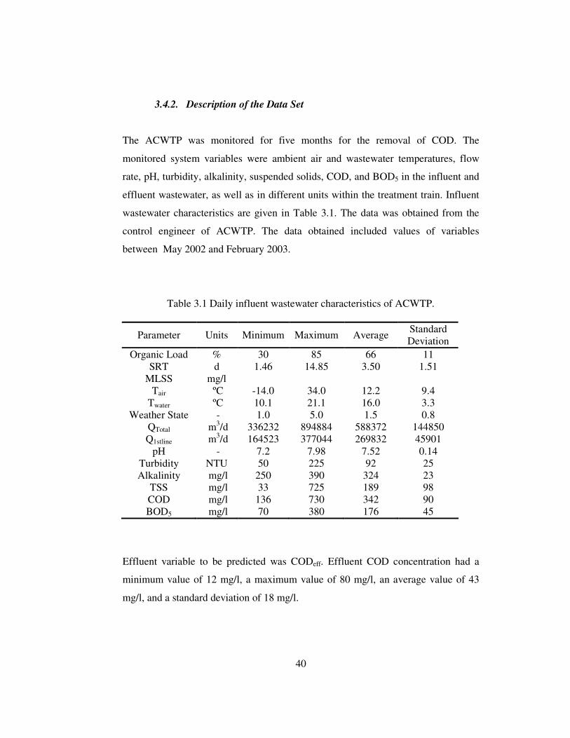
40
3.4.2. Description of the Data Set
The ACWTP was monitored for five months for the removal of COD. The
monitored system variables were ambient air and wastewater temperatures, flow
rate, pH, turbidity, alkalinity, suspended solids, COD, and BOD5 in the influent and
effluent wastewater, as well as in different units within the treatment train. Influent
wastewater characteristics are given in Table 3.1. The data was obtained from the
control engineer of ACWTP. The data obtained included values of variables
between May 2002 and February 2003.
Table 3.1 Daily influent wastewater characteristics of ACWTP.
Parameter Units Minimum Maximum Average Standard Deviation
Organic Load % 30 85 66 11 SRT d 1.46 14.85 3.50 1.51
MLSS mg/l Tair ºC -14.0 34.0 12.2 9.4
Twater ºC 10.1 21.1 16.0 3.3 Weather State - 1.0 5.0 1.5 0.8
QTotal m3/d 336232 894884 588372 144850 Q1stline m3/d 164523 377044 269832 45901
pH - 7.2 7.98 7.52 0.14 Turbidity NTU 50 225 92 25 Alkalinity mg/l 250 390 324 23
TSS mg/l 33 725 189 98 COD mg/l 136 730 342 90 BOD5 mg/l 70 380 176 45
Effluent variable to be predicted was CODeff. Effluent COD concentration had a
minimum value of 12 mg/l, a maximum value of 80 mg/l, an average value of 43
mg/l, and a standard deviation of 18 mg/l.

41
3.5. skenderun Wastewater Treatment Plant
skenderun Wastewater Treatment Plant is a high technology plant. The plant is a
fully automated where process control is administered via SCADA control.
3.5.1. Treatment Plant Layout & Dimensions
skenderun Wastewater Treatment Plant (IskWTP) process train is composed of
coarse and fine screens, grid removal, primary sedimentation tanks, activated sludge
aeration tanks, and secondary sedimentation tanks. The excess sludge produced in
the treatment plant is aerobically digested and dewatered. The design capacity of the
treatment plant is 57000 m3/d, however a capacity of 30000 m3/d had been used by
the end of 2003. The receiving body of the treated water is the Mediterranean Sea.
3.5.2. Description of the Data Set
Two different sets of data belonging to two different time periods were used in this
study. The first data set was for March 2002 to December 2002. The second data set
was for January 2003 to May 2003. The second data set was used for the model
development in this study.
Raw wastewater characteristics of the second data set are given in Table 3.2. There
were 33 parameters in the data obtained for the wastewater treatment plant but only
11 were used in model building. This low usage was because either the data were
blank or the data was unrelated with the process. The data used for the IskWTP was
obtained from the control engineer of the plant.
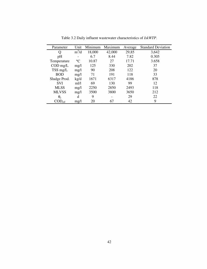
42
Table 3.2 Daily influent wastewater characteristics of IskWTP.
Parameter Unit Minimum Maximum Average Standard Deviation Q m3/d 18,000 42,000 29,85 3,642 pH - 6.7 8.44 7.82 0.305
Temperature °C 10.87 27 17.71 3.658 COD mg/L mg/l 125 330 202 37 TSS mg/L mg/l 90 208 122 20
BOD mg/l 71 191 118 33 Sludge Prod. kg/d 1671 6317 4186 878
SVI ml/l 69 130 99 12 MLSS mg/l 2250 2850 2493 118
MLVSS mg/l 3500 3800 3650 212 θc d 9 - 29 22
CODeff mg/l 20 67 42 9
43
CHAPTER IV
4. RESULTS AND DISCUSSION
In this study, three activated sludge-type treatment plants were modeled by using
ANN technique. One of the plants was a hypothetical wastewater treatment plant
developed by using SSSP v1.0 simulator (Simulation of Single-Sludge Processes for
Carbon Oxidation, Nitrification and Denitrification © 1984 Clemson University).
The other two were actual plants operating in Ankara and skenderun cities in
Turkey.
The hypothetical wastewater treatment plant was constructed by using SSSP’s
default parameters and default dynamic influent wastewater data representing a very
simple wastewater treatment plant. The default data was run in SSSP and dependent
variable values were obtained for the effluent. The default influent data was based
on average wastewater hourly characteristics observed in United States of America.
The hourly flow variation in the input file was also based on average USA
wastewater with 1000 m3/d flow rate. Then, a sensitivity analysis was carried out
on both SSSP and the constructed ANN model. Both outcomes were then compared
to determine the generalization ability of the ANN model.
In the second part of the study, ANN Models for two actual wastewater treatment
plants were developed with the data obtained from these plants. A MATLAB Script
was written to have an automated search process in the error surface aiming to
determine the minimum error on the predictions of the trained model.
44
4.1. SSSP Model Studies
4.1.1. The SSSP Simulation Program as a Hypothetical Wastewater
Treatment Plant
The hypothetical wastewater treatment plant present as default in the SSSP
simulation program was used as the first step for the development of an ANN model
for the sake of simplicity of data generation, applicability to the model, and for
quick output generation.
Another reason for the selection of SSSP simulation program is that, the program
uses the acclaimed ASM1 (Activated Sludge Model No 1) model which is currently
believed that it accurately describes some of the basic biological mechanisms
underlying in the activated sludge process. In addition, using a mechanistic model
simulator generates as much data needed for the training of an ANN model. The
SSSP model has already been used with success for the modeling of ACWTP
Ankara Central Wastewater Treatment Plant) and results have been published in the
literature by Sin (Sin, 2000).
The data used in the model development process is given in Table A.1. The output
of the SSSP program corresponding to the data set is given in Table A.2. These
influent-effluent data pairs were used in the ANN model development for the
hypothetical wastewater treatment plant. The input data set used in ANN model
building was consisted of variables of Q, Xs, Xi. In response, the ANN model
returned effluent variables of MLVSS, Ss, Xhet.
Input and output variable definitions of the SSSP program were given in Section
3.5.1. The effluent variable data computed by the SSSP program was produced a
data set with 30 min intervals, starting at 00:00 hour and ending at 24:00 hours.
Thus, the resulting daily data set consisted of 50 data points. However, the number
of data was reduced to 24 for use in the ANN modeling by linear interpolation. This

45
was done by taking average of each two consecutive values. The reason for this was
the need to supply the corresponding pairs of inputs and outputs for the ANN model
development.
The SSSP Hypothetical Wastewater Treatment Plant was established using the
default parameters in the SSSP Program. There are three aeration tanks, each of
which has a volume of 200 m3 and an average daily wastewater flow of 1000
m3/day fed to the system. The solids retention time (θc) is accepted as 10 days.
Dissolved oxygen concentration in each tank is assumed to be 4 mg/l. A recycle
input of 500 m3/d is given to the first aeration tank to which all the influent flow is
directed.
The graphical output of SSSP using the test input data for the selected variables are
given in Figures 4.1, 4.2, and 4.3.
Figure 4.1 MLVSS output of the SSSP simulation.
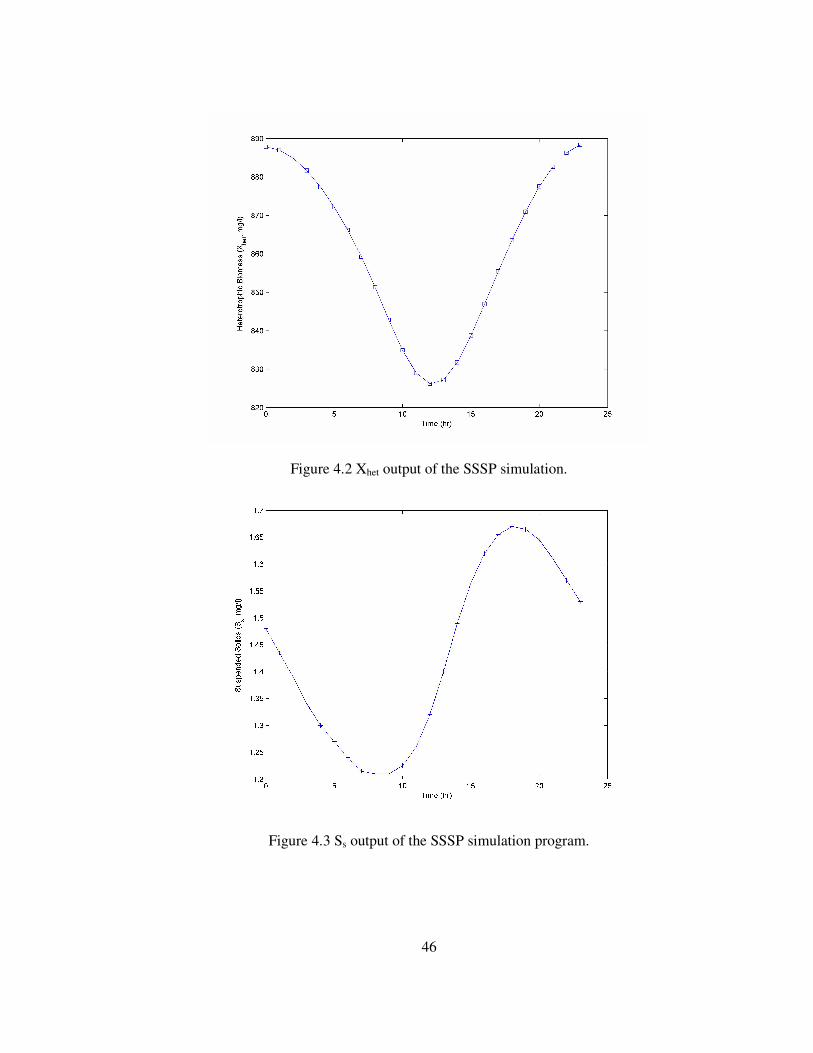
46
Figure 4.2 Xhet output of the SSSP simulation.
Figure 4.3 Ss output of the SSSP simulation program.
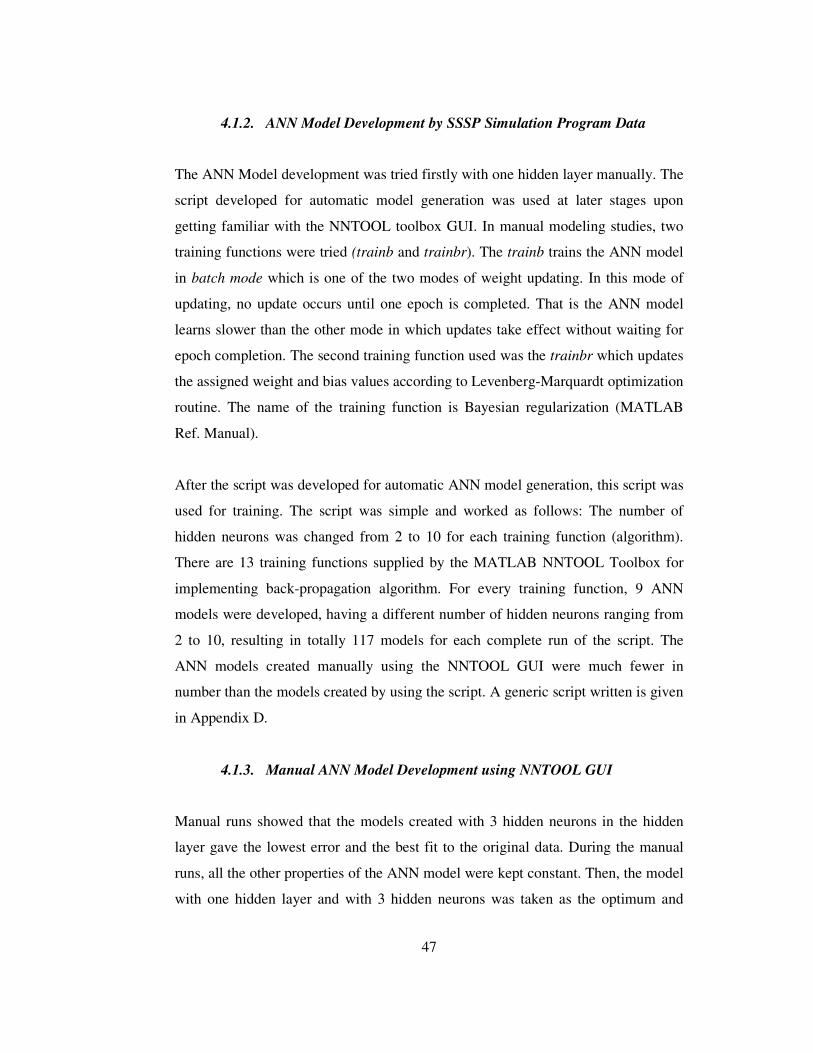
47
4.1.2. ANN Model Development by SSSP Simulation Program Data
The ANN Model development was tried firstly with one hidden layer manually. The
script developed for automatic model generation was used at later stages upon
getting familiar with the NNTOOL toolbox GUI. In manual modeling studies, two
training functions were tried (trainb and trainbr). The trainb trains the ANN model
in batch mode which is one of the two modes of weight updating. In this mode of
updating, no update occurs until one epoch is completed. That is the ANN model
learns slower than the other mode in which updates take effect without waiting for
epoch completion. The second training function used was the trainbr which updates
the assigned weight and bias values according to Levenberg-Marquardt optimization
routine. The name of the training function is Bayesian regularization (MATLAB
Ref. Manual).
After the script was developed for automatic ANN model generation, this script was
used for training. The script was simple and worked as follows: The number of
hidden neurons was changed from 2 to 10 for each training function (algorithm).
There are 13 training functions supplied by the MATLAB NNTOOL Toolbox for
implementing back-propagation algorithm. For every training function, 9 ANN
models were developed, having a different number of hidden neurons ranging from
2 to 10, resulting in totally 117 models for each complete run of the script. The
ANN models created manually using the NNTOOL GUI were much fewer in
number than the models created by using the script. A generic script written is given
in Appendix D.
4.1.3. Manual ANN Model Development using NNTOOL GUI
Manual runs showed that the models created with 3 hidden neurons in the hidden
layer gave the lowest error and the best fit to the original data. During the manual
runs, all the other properties of the ANN model were kept constant. Then, the model
with one hidden layer and with 3 hidden neurons was taken as the optimum and
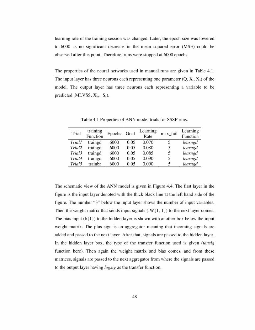
48
learning rate of the training session was changed. Later, the epoch size was lowered
to 6000 as no significant decrease in the mean squared error (MSE) could be
observed after this point. Therefore, runs were stopped at 6000 epochs.
The properties of the neural networks used in manual runs are given in Table 4.1.
The input layer has three neurons each representing one parameter (Q, Xi, Xs) of the
model. The output layer has three neurons each representing a variable to be
predicted (MLVSS, Xhet, Ss).
Table 4.1 Properties of ANN model trials for SSSP runs.
Trial training Function Epochs Goal Learning
Rate max_fail Learning Function
Trial1 traingd 6000 0.05 0.070 5 learngd Trial2 traingd 6000 0.05 0.080 5 learngd Trial3 traingd 6000 0.05 0.085 5 learngd Trial4 traingd 6000 0.05 0.090 5 learngd Trial5 trainbr 6000 0.05 0.090 5 learngd
The schematic view of the ANN model is given in Figure 4.4. The first layer in the
figure is the input layer denoted with the thick black line at the left hand side of the
figure. The number “3” below the input layer shows the number of input variables.
Then the weight matrix that sends input signals (IW1, 1) to the next layer comes.
The bias input (b1) to the hidden layer is shown with another box below the input
weight matrix. The plus sign is an aggregator meaning that incoming signals are
added and passed to the next layer. After that, signals are passed to the hidden layer.
In the hidden layer box, the type of the transfer function used is given (tansig
function here). Then again the weight matrix and bias comes, and from these
matrices, signals are passed to the next aggregator from where the signals are passed
to the output layer having logsig as the transfer function.
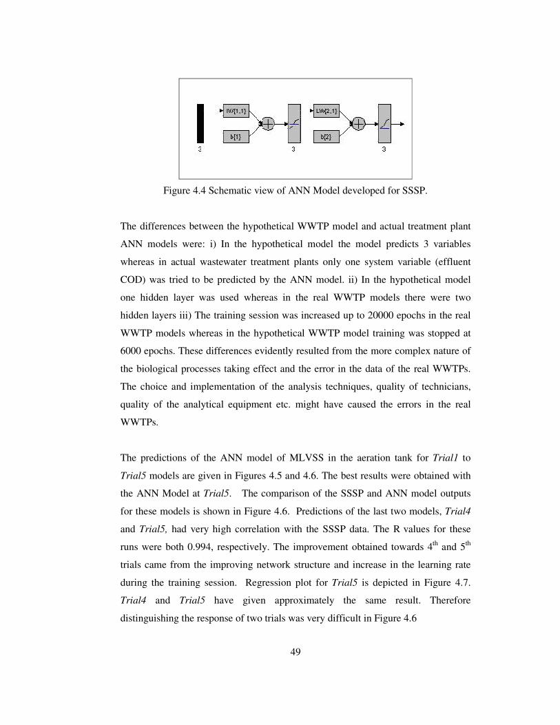
49
Figure 4.4 Schematic view of ANN Model developed for SSSP.
The differences between the hypothetical WWTP model and actual treatment plant
ANN models were: i) In the hypothetical model the model predicts 3 variables
whereas in actual wastewater treatment plants only one system variable (effluent
COD) was tried to be predicted by the ANN model. ii) In the hypothetical model
one hidden layer was used whereas in the real WWTP models there were two
hidden layers iii) The training session was increased up to 20000 epochs in the real
WWTP models whereas in the hypothetical WWTP model training was stopped at
6000 epochs. These differences evidently resulted from the more complex nature of
the biological processes taking effect and the error in the data of the real WWTPs.
The choice and implementation of the analysis techniques, quality of technicians,
quality of the analytical equipment etc. might have caused the errors in the real
WWTPs.
The predictions of the ANN model of MLVSS in the aeration tank for Trial1 to
Trial5 models are given in Figures 4.5 and 4.6. The best results were obtained with
the ANN Model at Trial5. The comparison of the SSSP and ANN model outputs
for these models is shown in Figure 4.6. Predictions of the last two models, Trial4
and Trial5, had very high correlation with the SSSP data. The R values for these
runs were both 0.994, respectively. The improvement obtained towards 4th and 5th
trials came from the improving network structure and increase in the learning rate
during the training session. Regression plot for Trial5 is depicted in Figure 4.7.
Trial4 and Trial5 have given approximately the same result. Therefore
distinguishing the response of two trials was very difficult in Figure 4.6
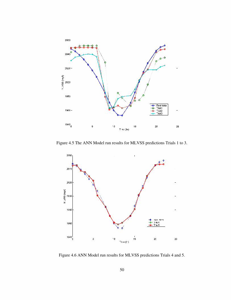
50
Figure 4.5 The ANN Model run results for MLVSS predictions Trials 1 to 3.
Figure 4.6 ANN Model run results for MLVSS predictions Trials 4 and 5.
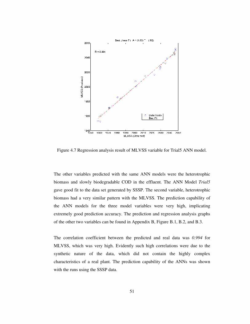
51
Figure 4.7 Regression analysis result of MLVSS variable for Trial5 ANN model.
The other variables predicted with the same ANN models were the heterotrophic
biomass and slowly biodegradable COD in the effluent. The ANN Model Trial5
gave good fit to the data set generated by SSSP. The second variable, heterotrophic
biomass had a very similar pattern with the MLVSS. The prediction capability of
the ANN models for the three model variables were very high, implicating
extremely good prediction accuracy. The prediction and regression analysis graphs
of the other two variables can be found in Appendix B, Figure B.1, B.2, and B.3.
The correlation coefficient between the predicted and real data was 0.994 for
MLVSS, which was very high. Evidently such high correlations were due to the
synthetic nature of the data, which did not contain the highly complex
characteristics of a real plant. The prediction capability of the ANNs was shown
with the runs using the SSSP data.
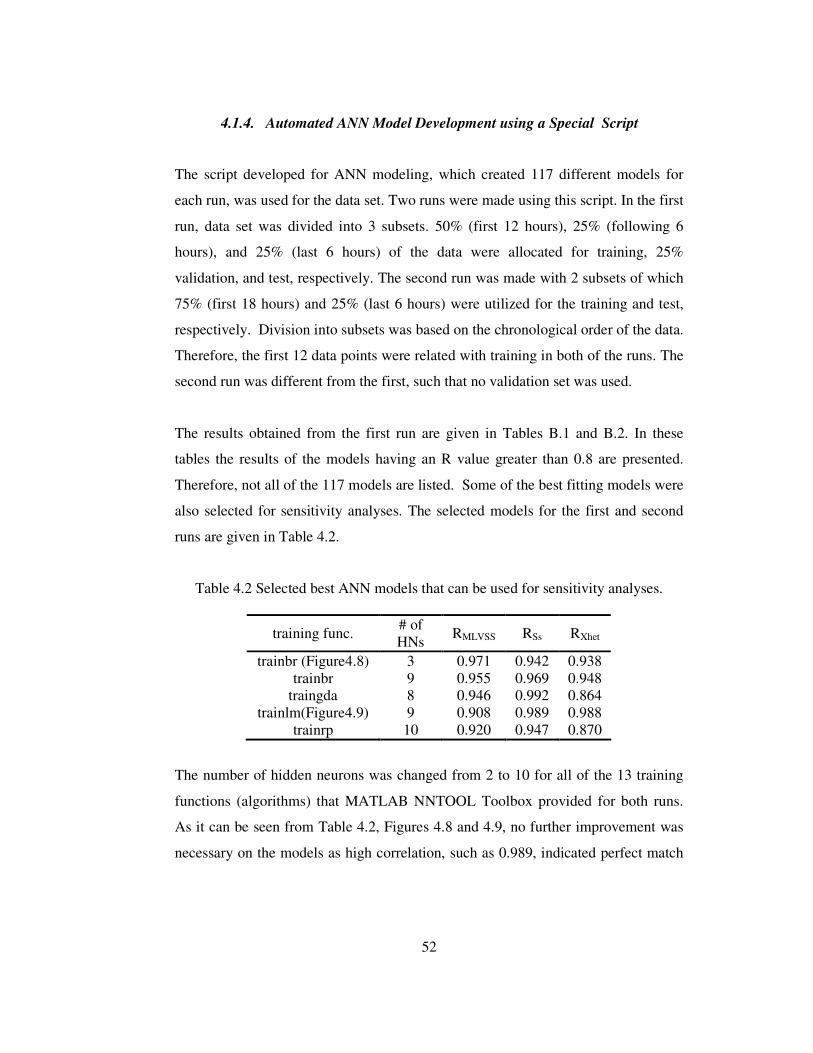
52
4.1.4. Automated ANN Model Development using a Special Script
The script developed for ANN modeling, which created 117 different models for
each run, was used for the data set. Two runs were made using this script. In the first
run, data set was divided into 3 subsets. 50% (first 12 hours), 25% (following 6
hours), and 25% (last 6 hours) of the data were allocated for training, 25%
validation, and test, respectively. The second run was made with 2 subsets of which
75% (first 18 hours) and 25% (last 6 hours) were utilized for the training and test,
respectively. Division into subsets was based on the chronological order of the data.
Therefore, the first 12 data points were related with training in both of the runs. The
second run was different from the first, such that no validation set was used.
The results obtained from the first run are given in Tables B.1 and B.2. In these
tables the results of the models having an R value greater than 0.8 are presented.
Therefore, not all of the 117 models are listed. Some of the best fitting models were
also selected for sensitivity analyses. The selected models for the first and second
runs are given in Table 4.2.
Table 4.2 Selected best ANN models that can be used for sensitivity analyses.
training func. # of HNs RMLVSS RSs RXhet
trainbr (Figure4.8) 3 0.971 0.942 0.938 trainbr 9 0.955 0.969 0.948
traingda 8 0.946 0.992 0.864 trainlm(Figure4.9) 9 0.908 0.989 0.988
trainrp 10 0.920 0.947 0.870
The number of hidden neurons was changed from 2 to 10 for all of the 13 training
functions (algorithms) that MATLAB NNTOOL Toolbox provided for both runs.
As it can be seen from Table 4.2, Figures 4.8 and 4.9, no further improvement was
necessary on the models as high correlation, such as 0.989, indicated perfect match
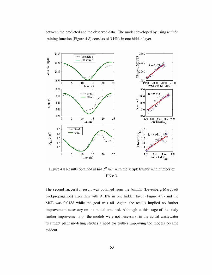
53
between the predicted and the observed data. The model developed by using trainbr
training function (Figure 4.8) consists of 3 HNs in one hidden layer.
Figure 4.8 Results obtained in the 1st run with the script: trainbr with number of
HNs: 3.
The second successful result was obtained from the trainlm (Levenberg-Marquadt
backpropagation) algorithm with 9 HNs in one hidden layer (Figure 4.9) and the
MSE was 0.0188 while the goal was nil. Again, the results implied no further
improvement necessary on the model obtained. Although at this stage of the study
further improvements on the models were not necessary, in the actual wastewater
treatment plant modeling studies a need for further improving the models became
evident.
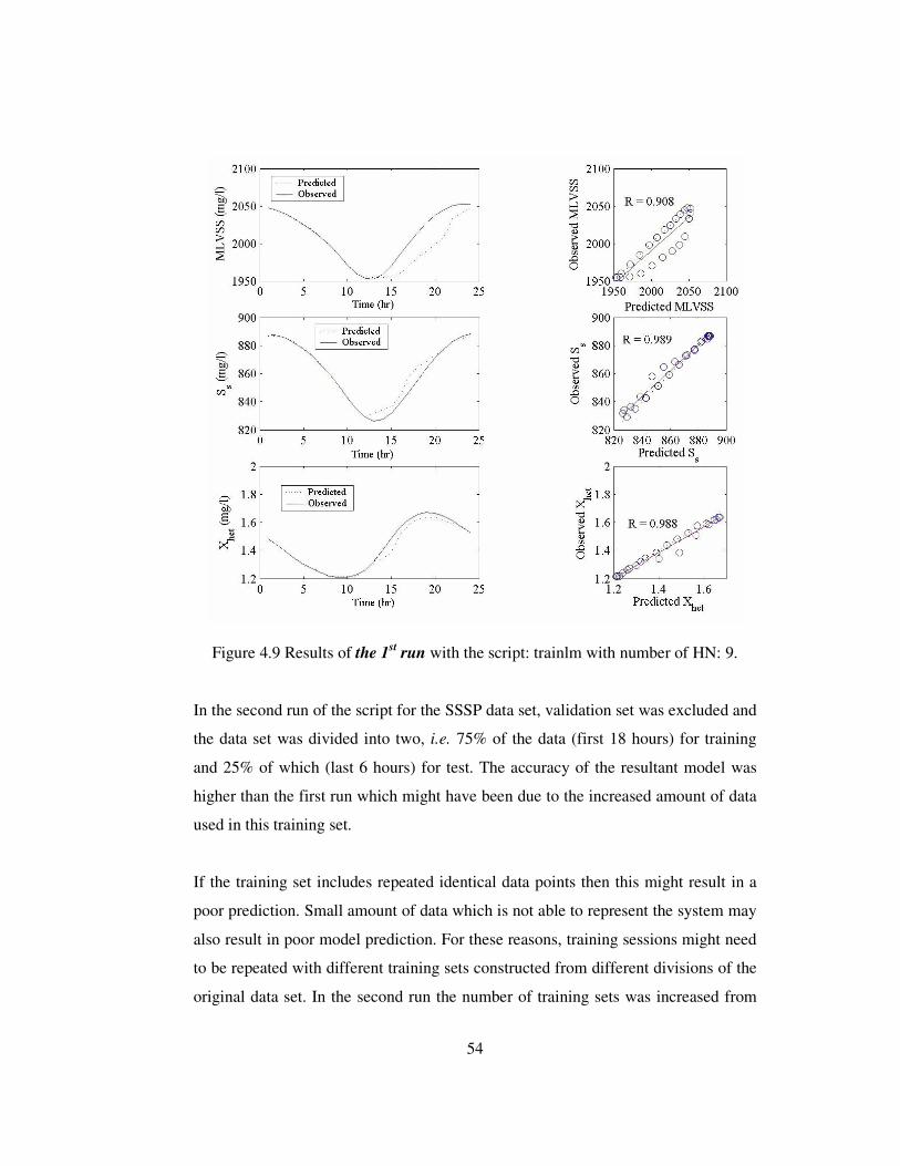
54
Figure 4.9 Results of the 1st run with the script: trainlm with number of HN: 9.
In the second run of the script for the SSSP data set, validation set was excluded and
the data set was divided into two, i.e. 75% of the data (first 18 hours) for training
and 25% of which (last 6 hours) for test. The accuracy of the resultant model was
higher than the first run which might have been due to the increased amount of data
used in this training set.
If the training set includes repeated identical data points then this might result in a
poor prediction. Small amount of data which is not able to represent the system may
also result in poor model prediction. For these reasons, training sessions might need
to be repeated with different training sets constructed from different divisions of the
original data set. In the second run the number of training sets was increased from

55
50% to 75% of the data and the remaining data was used for testing the goodness of
fit.
Four of the best models selected are given in Table 4.3. The second model (traingda
with 10 hidden neurons) was later used in sensitivity analysis. Figures 4.10 and 4.11
show the responses of the ANN models developed using the traincgp with 4 HNs,
and traingda with 10 HNs, respectively.
Figure 4.10 The results of the 2nd run with the script; using traincgp with four
number of HN
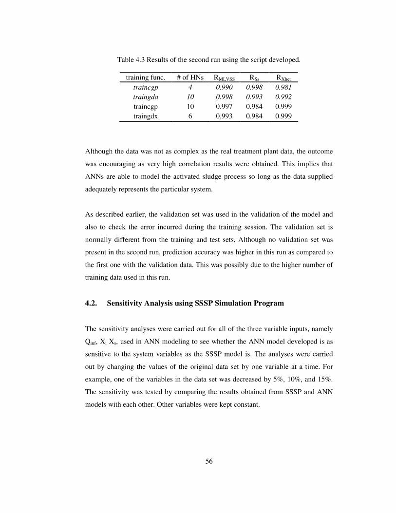
56
Table 4.3 Results of the second run using the script developed.
training func. # of HNs RMLVSS RSs RXhet traincgp 4 0.990 0.998 0.981 traingda 10 0.998 0.993 0.992 traincgp 10 0.997 0.984 0.999 traingdx 6 0.993 0.984 0.999
Although the data was not as complex as the real treatment plant data, the outcome
was encouraging as very high correlation results were obtained. This implies that
ANNs are able to model the activated sludge process so long as the data supplied
adequately represents the particular system.
As described earlier, the validation set was used in the validation of the model and
also to check the error incurred during the training session. The validation set is
normally different from the training and test sets. Although no validation set was
present in the second run, prediction accuracy was higher in this run as compared to
the first one with the validation data. This was possibly due to the higher number of
training data used in this run.
4.2. Sensitivity Analysis using SSSP Simulation Program
The sensitivity analyses were carried out for all of the three variable inputs, namely
Qinf, Xi Xs, used in ANN modeling to see whether the ANN model developed is as
sensitive to the system variables as the SSSP model is. The analyses were carried
out by changing the values of the original data set by one variable at a time. For
example, one of the variables in the data set was decreased by 5%, 10%, and 15%.
The sensitivity was tested by comparing the results obtained from SSSP and ANN
models with each other. Other variables were kept constant.
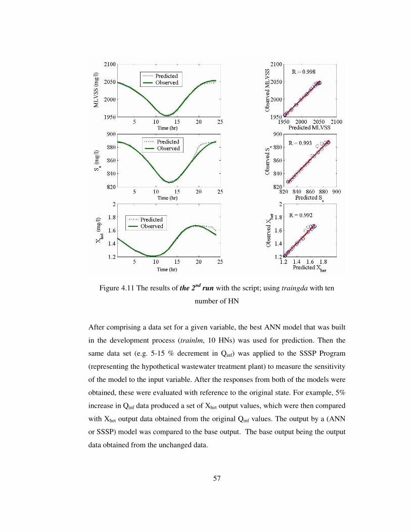
57
Figure 4.11 The results of the 2nd run with the script; using traingda with ten
number of HN
After comprising a data set for a given variable, the best ANN model that was built
in the development process (trainlm, 10 HNs) was used for prediction. Then the
same data set (e.g. 5-15 % decrement in Qınf) was applied to the SSSP Program
(representing the hypothetical wastewater treatment plant) to measure the sensitivity
of the model to the input variable. After the responses from both of the models were
obtained, these were evaluated with reference to the original state. For example, 5%
increase in Qinf data produced a set of Xhet output values, which were then compared
with Xhet output data obtained from the original Qinf values. The output by a (ANN
or SSSP) model was compared to the base output. The base output being the output
data obtained from the unchanged data.
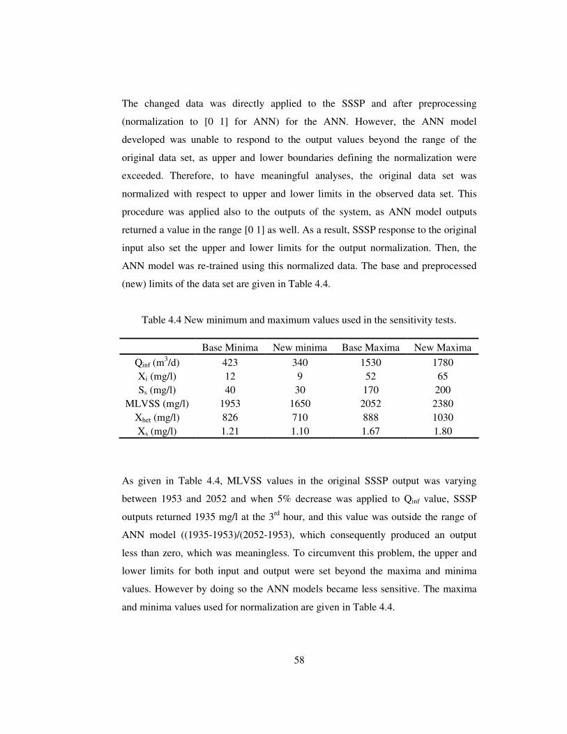
58
The changed data was directly applied to the SSSP and after preprocessing
(normalization to [0 1] for ANN) for the ANN. However, the ANN model
developed was unable to respond to the output values beyond the range of the
original data set, as upper and lower boundaries defining the normalization were
exceeded. Therefore, to have meaningful analyses, the original data set was
normalized with respect to upper and lower limits in the observed data set. This
procedure was applied also to the outputs of the system, as ANN model outputs
returned a value in the range [0 1] as well. As a result, SSSP response to the original
input also set the upper and lower limits for the output normalization. Then, the
ANN model was re-trained using this normalized data. The base and preprocessed
(new) limits of the data set are given in Table 4.4.
Table 4.4 New minimum and maximum values used in the sensitivity tests.
Base Minima New minima Base Maxima New Maxima Qinf (m3/d) 423 340 1530 1780 Xi (mg/l) 12 9 52 65 Ss (mg/l) 40 30 170 200
MLVSS (mg/l) 1953 1650 2052 2380 Xhet (mg/l) 826 710 888 1030 Xs (mg/l) 1.21 1.10 1.67 1.80
As given in Table 4.4, MLVSS values in the original SSSP output was varying
between 1953 and 2052 and when 5% decrease was applied to Qinf value, SSSP
outputs returned 1935 mg/l at the 3rd hour, and this value was outside the range of
ANN model ((1935-1953)/(2052-1953), which consequently produced an output
less than zero, which was meaningless. To circumvent this problem, the upper and
lower limits for both input and output were set beyond the maxima and minima
values. However by doing so the ANN models became less sensitive. The maxima
and minima values used for normalization are given in Table 4.4.
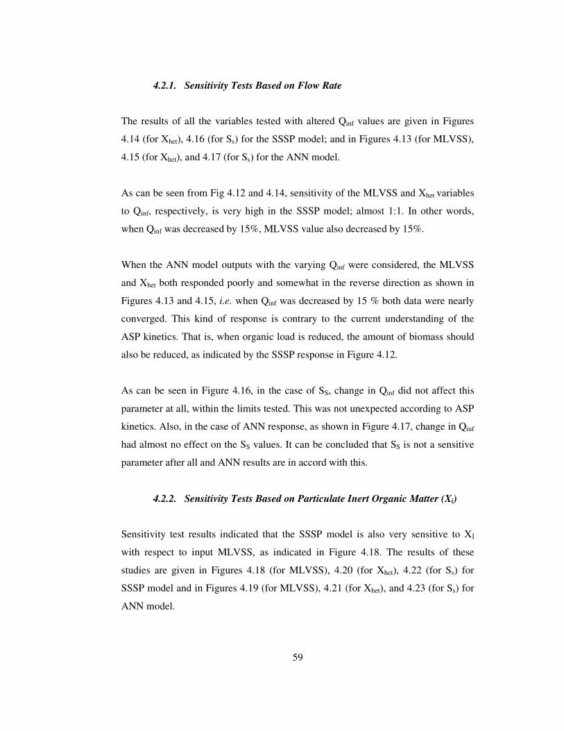
59
4.2.1. Sensitivity Tests Based on Flow Rate
The results of all the variables tested with altered Qinf values are given in Figures
4.14 (for Xhet), 4.16 (for Ss) for the SSSP model; and in Figures 4.13 (for MLVSS),
4.15 (for Xhet), and 4.17 (for Ss) for the ANN model.
As can be seen from Fig 4.12 and 4.14, sensitivity of the MLVSS and Xhet variables
to Qinf, respectively, is very high in the SSSP model; almost 1:1. In other words,
when Qinf was decreased by 15%, MLVSS value also decreased by 15%.
When the ANN model outputs with the varying Qinf were considered, the MLVSS
and Xhet both responded poorly and somewhat in the reverse direction as shown in
Figures 4.13 and 4.15, i.e. when Qinf was decreased by 15 % both data were nearly
converged. This kind of response is contrary to the current understanding of the
ASP kinetics. That is, when organic load is reduced, the amount of biomass should
also be reduced, as indicated by the SSSP response in Figure 4.12.
As can be seen in Figure 4.16, in the case of SS, change in Qinf did not affect this
parameter at all, within the limits tested. This was not unexpected according to ASP
kinetics. Also, in the case of ANN response, as shown in Figure 4.17, change in Qinf
had almost no effect on the SS values. It can be concluded that SS is not a sensitive
parameter after all and ANN results are in accord with this.
4.2.2. Sensitivity Tests Based on Particulate Inert Organic Matter (Xi)
Sensitivity test results indicated that the SSSP model is also very sensitive to X
with respect to input MLVSS, as indicated in Figure 4.18. The results of these
studies are given in Figures 4.18 (for MLVSS), 4.20 (for Xhet), 4.22 (for Ss) for
SSSP model and in Figures 4.19 (for MLVSS), 4.21 (for Xhet), and 4.23 (for Ss) for
ANN model.

60
It can be concluded that response of ANN to Xi input with respect to MLVSS was
somewhat close to that obtained in SSSP, as indicated in Figure 4.18. It can be
concluded that the results might improve using dedicated ANN models for each
output variables i.e. MLVSS, Xhet, and Ss. Here, three input variables are entered
into the model and three variable outputs are received. In a dedicated model three
variables may be entered but one variable output may be obtained.
Another reason for the poor prediction of the ANN model could be due to the
altered model limits which were changed in the sensitivity data set to avoid minus
normalization. This has resulted in the accumulation of the original data set between
[0.38 - 0.55] range, which might have resulted in poor training.
Figure 4.12 Sensitivity test results of MLVSS for SSSP Hypothetical WWTP for
changed Qinf.
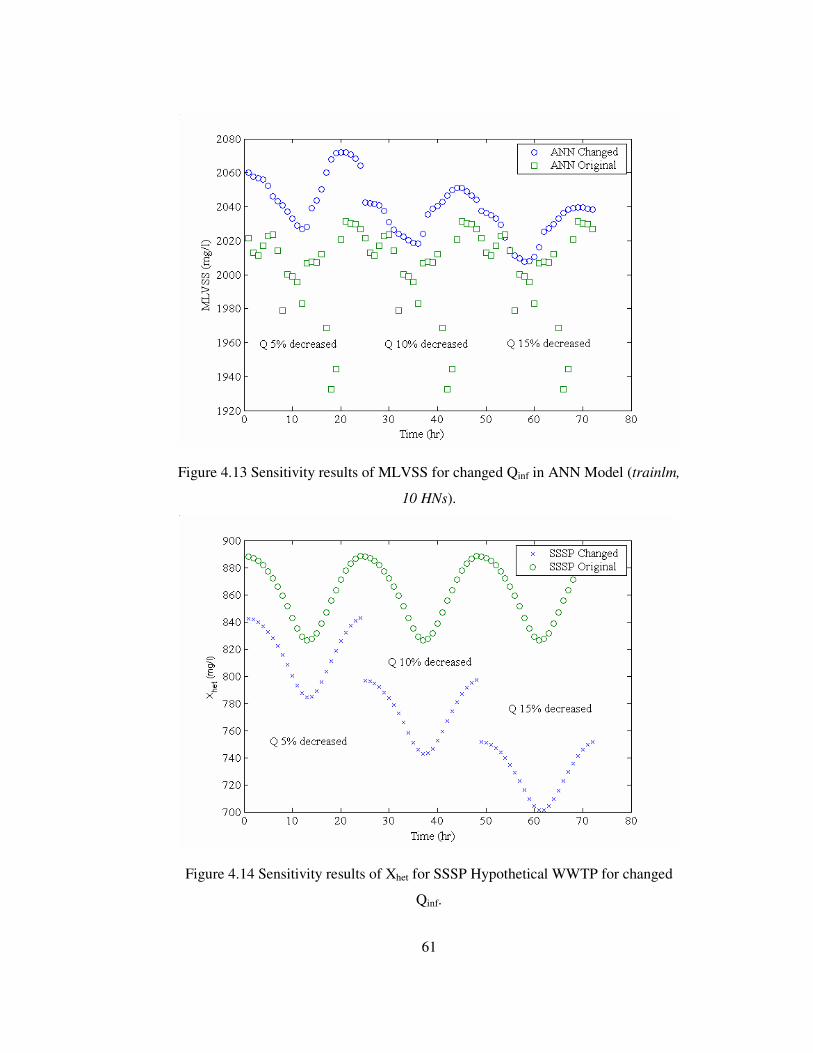
61
Figure 4.13 Sensitivity results of MLVSS for changed Qinf in ANN Model (trainlm,
10 HNs).
Figure 4.14 Sensitivity results of Xhet for SSSP Hypothetical WWTP for changed
Qinf.
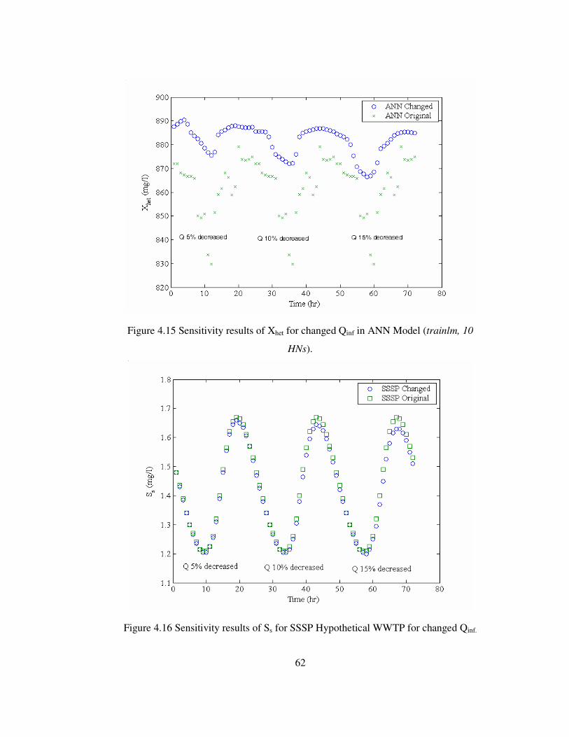
62
Figure 4.15 Sensitivity results of Xhet for changed Qinf in ANN Model (trainlm, 10
HNs).
Figure 4.16 Sensitivity results of Ss for SSSP Hypothetical WWTP for changed Qinf.
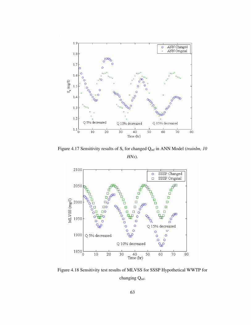
63
Figure 4.17 Sensitivity results of Ss for changed Qinf in ANN Model (trainlm, 10
HNs).
Figure 4.18 Sensitivity test results of MLVSS for SSSP Hypothetical WWTP for
changing Qinf.

64
Figure 4.19 Sensitivity results of MLVSS for changed Qinf in ANN Model (trainlm,
10 HNs).
Figure 4.20 Sensitivity results of Xhet for SSSP Hypothetical WWTP for changed Xi.
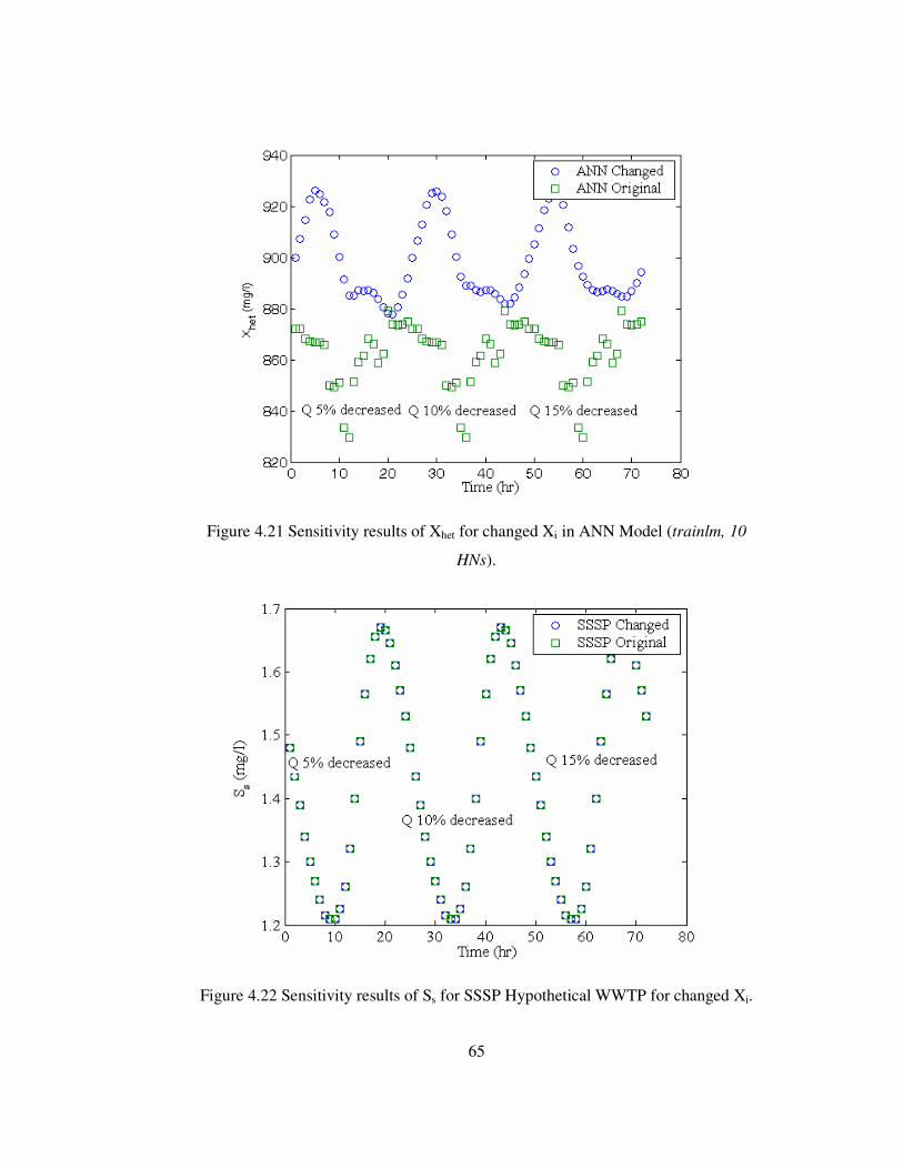
65
Figure 4.21 Sensitivity results of Xhet for changed Xi in ANN Model (trainlm, 10
HNs).
Figure 4.22 Sensitivity results of Ss for SSSP Hypothetical WWTP for changed Xi.

66
Figure 4.23 Sensitivity results of Ss for changed Xi in ANN Model (trainlm, 10
HNs).
4.3. ANN Modeling Studies with skenderun Wastewater Treatment
Plant (IskWTP) Data
4.3.1. IskWTP Data Preparation
Two different data sets were used for ANN modeling of IskWTP. These were
belonging to the period from March 2002 to December 2002, and from January
2003 to May 2003. The first runs were made using the first set. However, the ANN
models developed using this data set gave poor predictions. The highest correlation
obtained was about 0.35. Then, the second set of data was used for model
development.

67
In the modeling process, 9 of the system variables were used to build an ANN
model. Also various combinations of the data were used in the model development
process. System variables that were used in the modeling process were solids
retention time (θc), influent flow rate (Qinf), influent pH, influent water temperature
(Tinf), influent COD concentration; MLSS, effluent COD, effluent TSS and sludge
production rate from the primary sedimentation tank. These variables, singly or in
combinations, were used to predict effluent COD concentration of the treated water
from the treatment plant. Numerous combinations of variables were used and
hundreds of models were developed and trained to see the efficacy of the prediction.
Only those models resulting in high efficacy will be presented here.
Preparation of data was executed by excluding blank values from the original data
set. Initially the raw data was composed of approximately 5 months of daily
measurements, excluding Sundays, and summing up to 108 days. There were blanks
in the data. Rows of data having blanks were removed completely from the set. For
example, number of points used in ANN model for the three variable combinations,
namely, effluent total suspended solids, MLSS of primary sedimentation tank and
influent flow rate, was 99; where 9 rows of data containing blanks in any of the
three variables were discarded.
4.3.2. IskWTP Data Preprocessing
After preparation of the data for the model development, preprocessing was carried
out to assign all the variables equal weights in the weight update process,
particularly when using a non-linear transfer function. The preprocessing was
established by conversion of the input and output data into the range [0 1] or [-1
+1].
This conversion was done for all the points in the data as follows:

68
For [0 1] range;
minmax
min
xxxx
X ii −
−= (4.1)
and for [-1 +1] range,
12minmax
min −−
−×=
xxxx
X ii (4.2)
Each variable in the data have to be supplied in equal weights to the ANN model by
normalizing the input data when nonlinear transfer functions like logsig, tansig were
being used. Therefore, the data have to be scaled into [0 1] or [-1 +1] range using
Equations 4.1 and 4.2, respectively.
In runs with [-1 +1] range, no good results were obtained. In these runs, firstly the
script with one hidden layer was tried. Then, the hidden neuron number was
changed using the criterion defined by Hecht and Nielsen (1987). The highest
correlation coefficients obtained in these runs were around 0.4.
Later, number of hidden layers was increased to 2. Using the same data and in the [0
1] range, the transfer function logsig and in the [-1 +1] range, the transfer function
tansig were used. It is possible to use transfer function combinations in multilayer
models by using a particular transfer function at one layer and another at different
layer(s). Some of the possible combinations of these functions when using two
hidden layers (tansig-tansig, logsig-logsig, tansig-purelin, … etc.).
4.3.3. IskWTP ANN Model Development
The MATLAB Script was used to construct ANN models automatically by using the
data for IskWTP. The implementation of the script started with the determination of
the combinations of the variables to be used together. Variable combinations used in
model development process are given in Table 4.6. These combinations were tried

69
in the given order until a good fits to the actual data were obtained by visual
judgment and by considering the correlation coefficient, R. When an acceptable fit
was reached, this was further improved by grouping the variables giving the best
results.
As can be seen in Table 4.6, the best fit to the effluent COD data was obtained with
the combination number 25, yielding R=0.795. Basing on this observation, the
variables identified in combination 25 were tested further singly or in pairs to create
new subsets to be used in the script, in search for improved results. The variable
combinations tested are presented in Table 4.5.
Table 4.5 Set descriptions for Combinations 25 and 26.
Set No Variable(s) used 1 MLSS only, 2 TSSeff only, 3 MLSS and Qinf, 4 Qinf and TSSeff, 5 Qinf, TSSeff and MLSS, 6 MLSS and TSSeff.
Table 4.6 Combinations of variables used in individual runs of the script.
No Qinf pHinf Tinf CODinf MLSS TSSeff ∆∆∆∆X θθθθc Best R 1 0.411 2 0.360 3 0.310 4 0.462 5 0.257 6 0.223 7 0.207 8 0.211 9 0.291
10 0.256 11 0.302 12 0.321 13 0.451
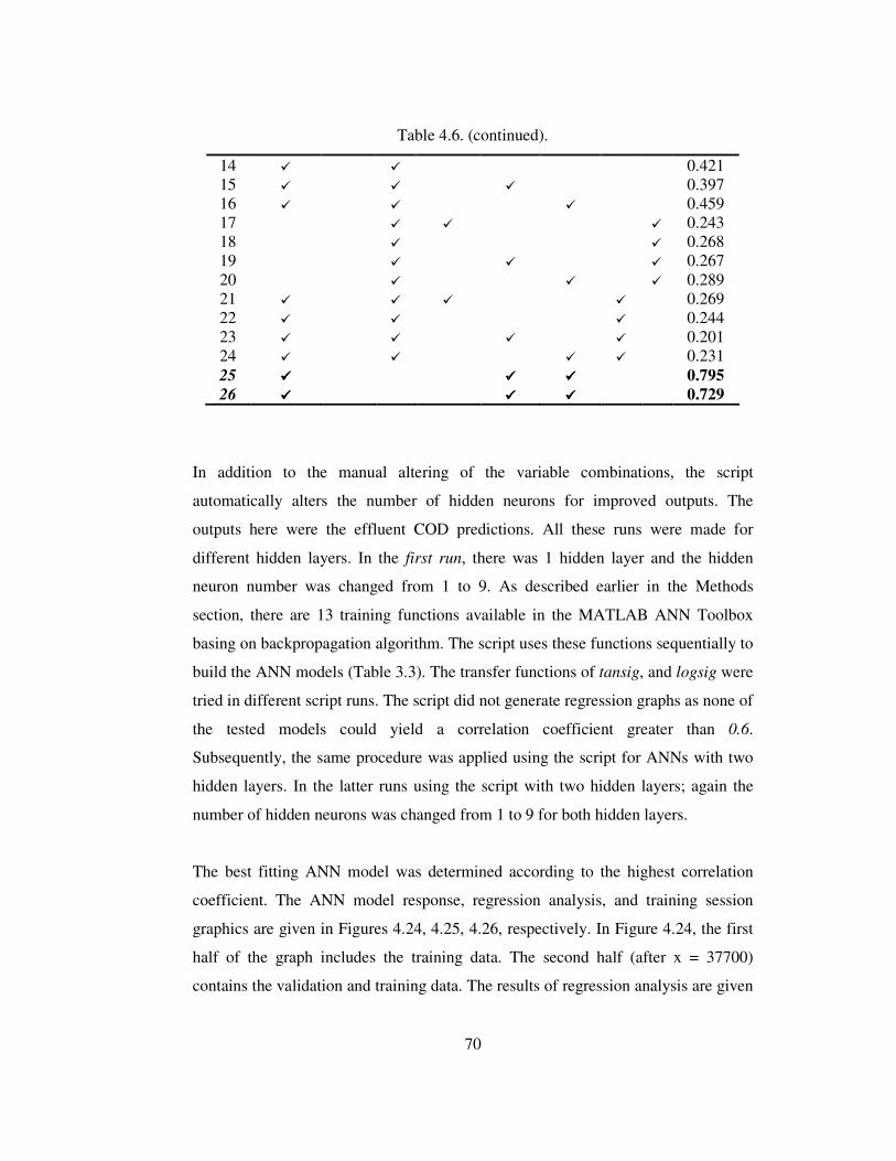
70
Table 4.6. (continued).
14 0.421 15 0.397 16 0.459 17 0.243 18 0.268 19 0.267 20 0.289 21 0.269 22 0.244 23 0.201 24 0.231 25 0.795 26 0.729
In addition to the manual altering of the variable combinations, the script
automatically alters the number of hidden neurons for improved outputs. The
outputs here were the effluent COD predictions. All these runs were made for
different hidden layers. In the first run, there was 1 hidden layer and the hidden
neuron number was changed from 1 to 9. As described earlier in the Methods
section, there are 13 training functions available in the MATLAB ANN Toolbox
basing on backpropagation algorithm. The script uses these functions sequentially to
build the ANN models (Table 3.3). The transfer functions of tansig, and logsig were
tried in different script runs. The script did not generate regression graphs as none of
the tested models could yield a correlation coefficient greater than 0.6.
Subsequently, the same procedure was applied using the script for ANNs with two
hidden layers. In the latter runs using the script with two hidden layers; again the
number of hidden neurons was changed from 1 to 9 for both hidden layers.
The best fitting ANN model was determined according to the highest correlation
coefficient. The ANN model response, regression analysis, and training session
graphics are given in Figures 4.24, 4.25, 4.26, respectively. In Figure 4.24, the first
half of the graph includes the training data. The second half (after x = 37700)
contains the validation and training data. The results of regression analysis are given
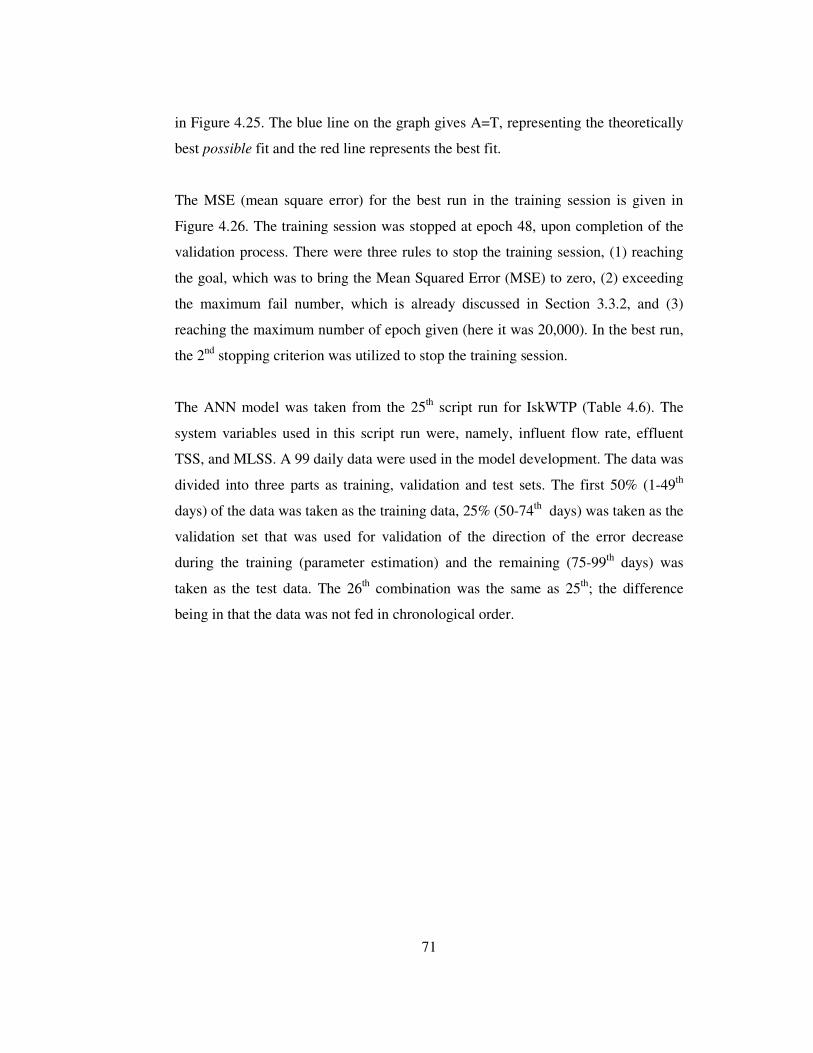
71
in Figure 4.25. The blue line on the graph gives A=T, representing the theoretically
best possible fit and the red line represents the best fit.
The MSE (mean square error) for the best run in the training session is given in
Figure 4.26. The training session was stopped at epoch 48, upon completion of the
validation process. There were three rules to stop the training session, (1) reaching
the goal, which was to bring the Mean Squared Error (MSE) to zero, (2) exceeding
the maximum fail number, which is already discussed in Section 3.3.2, and (3)
reaching the maximum number of epoch given (here it was 20,000). In the best run,
the 2nd stopping criterion was utilized to stop the training session.
The ANN model was taken from the 25th script run for IskWTP (Table 4.6). The
system variables used in this script run were, namely, influent flow rate, effluent
TSS, and MLSS. A 99 daily data were used in the model development. The data was
divided into three parts as training, validation and test sets. The first 50% (1-49th
days) of the data was taken as the training data, 25% (50-74th days) was taken as the
validation set that was used for validation of the direction of the error decrease
during the training (parameter estimation) and the remaining (75-99th days) was
taken as the test data. The 26th combination was the same as 25th; the difference
being in that the data was not fed in chronological order.
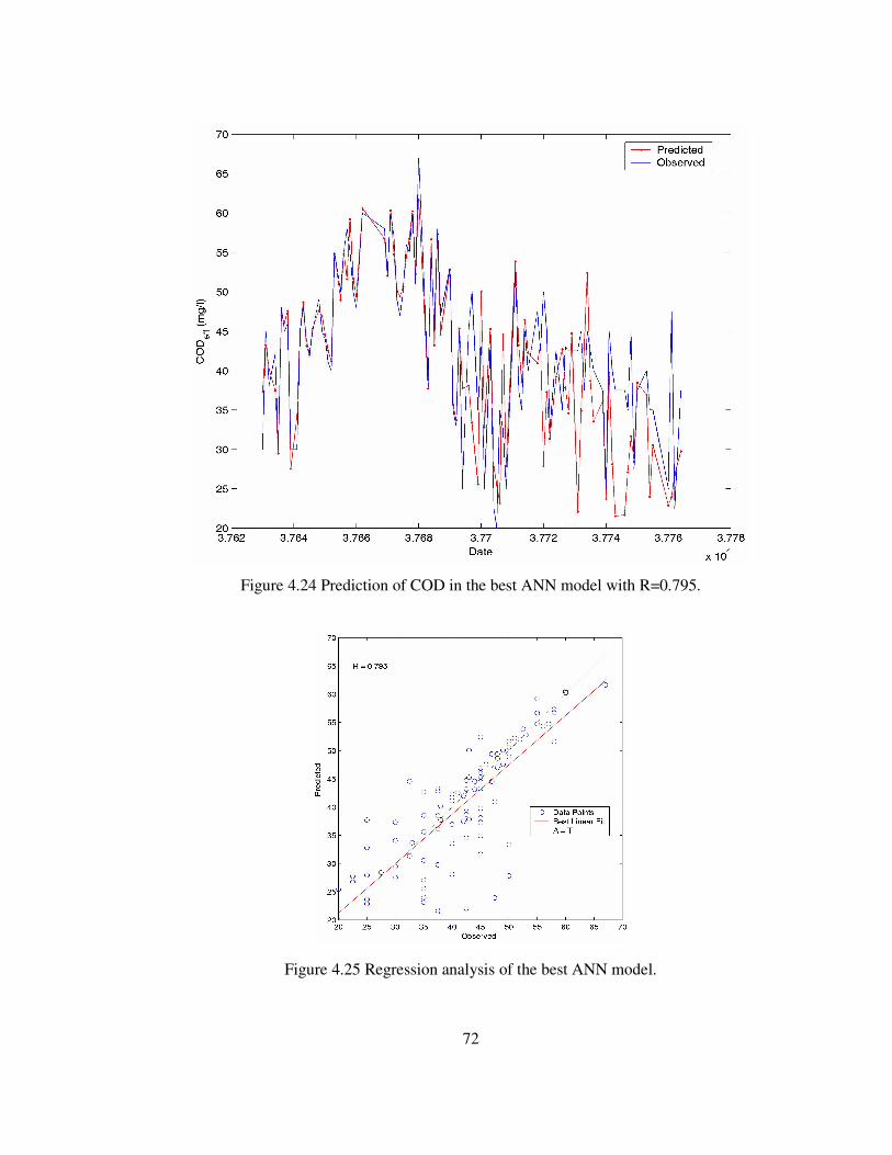
72
Figure 4.24 Prediction of COD in the best ANN model with R=0.795.
Figure 4.25 Regression analysis of the best ANN model.

73
Figure 4.26 Prediction of COD in the best ANN model with R=0.795
It can be seen in Figures 24, 25, and 26 that the results obtained were fairly good.
The best correlation coefficient obtained was 0.795. Results could have been even
better if the data used were more numerous and accurate. The data set used in this
study included too many blanks which interrupted a continuous data input to the
ANN model. The quality of daily data was unsure which increased uncertainty.
Although it is known that ANN can cope with noisy and erroneous data well, the
process parameters in biological wastewater treatment used in ANN modeling are
numerous and relative error is often high in these. Therefore the combination of
errors propagates during ANN modeling. Therefore, ideally the main purpose in
ANN modeling would be to predict objective variables using the data from
automatic sensors controlling the treatment plant. Random human error would be
minimized by this.
The best results obtained using the MATLAB Script, are given in Tables 4.7 and
4.8. In these tables, name of the backpropagation algorithm, variable set
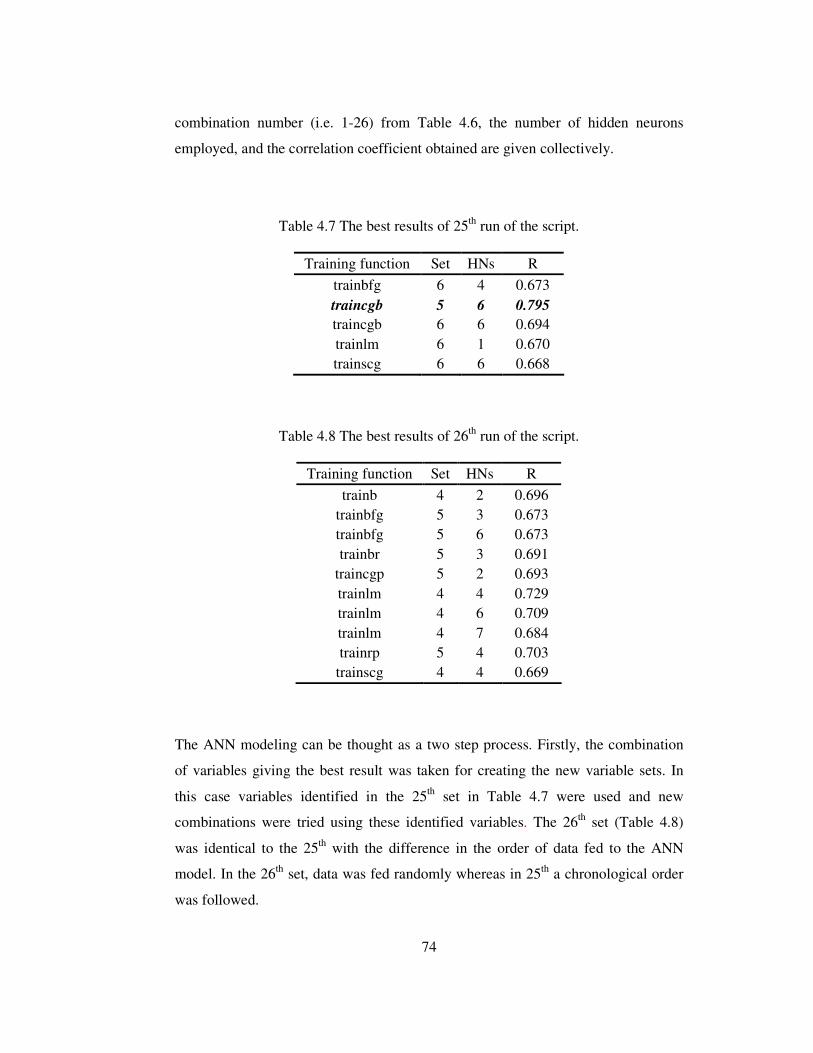
74
combination number (i.e. 1-26) from Table 4.6, the number of hidden neurons
employed, and the correlation coefficient obtained are given collectively.
Table 4.7 The best results of 25th run of the script.
Training function Set HNs R trainbfg 6 4 0.673 traincgb 5 6 0.795 traincgb 6 6 0.694 trainlm 6 1 0.670 trainscg 6 6 0.668
Table 4.8 The best results of 26th run of the script.
Training function Set HNs R trainb 4 2 0.696
trainbfg 5 3 0.673 trainbfg 5 6 0.673 trainbr 5 3 0.691
traincgp 5 2 0.693 trainlm 4 4 0.729 trainlm 4 6 0.709 trainlm 4 7 0.684 trainrp 5 4 0.703
trainscg 4 4 0.669
The ANN modeling can be thought as a two step process. Firstly, the combination
of variables giving the best result was taken for creating the new variable sets. In
this case variables identified in the 25th set in Table 4.7 were used and new
combinations were tried using these identified variables. The 26th set (Table 4.8)
was identical to the 25th with the difference in the order of data fed to the ANN
model. In the 26th set, data was fed randomly whereas in 25th a chronological order
was followed.
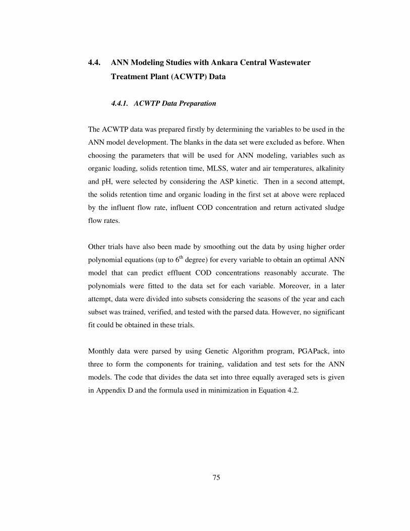
75
4.4. ANN Modeling Studies with Ankara Central Wastewater
Treatment Plant (ACWTP) Data
4.4.1. ACWTP Data Preparation
The ACWTP data was prepared firstly by determining the variables to be used in the
ANN model development. The blanks in the data set were excluded as before. When
choosing the parameters that will be used for ANN modeling, variables such as
organic loading, solids retention time, MLSS, water and air temperatures, alkalinity
and pH, were selected by considering the ASP kinetic. Then in a second attempt,
the solids retention time and organic loading in the first set at above were replaced
by the influent flow rate, influent COD concentration and return activated sludge
flow rates.
Other trials have also been made by smoothing out the data by using higher order
polynomial equations (up to 6th degree) for every variable to obtain an optimal ANN
model that can predict effluent COD concentrations reasonably accurate. The
polynomials were fitted to the data set for each variable. Moreover, in a later
attempt, data were divided into subsets considering the seasons of the year and each
subset was trained, verified, and tested with the parsed data. However, no significant
fit could be obtained in these trials.
Monthly data were parsed by using Genetic Algorithm program, PGAPack, into
three to form the components for training, validation and test sets for the ANN
models. The code that divides the data set into three equally averaged sets is given
in Appendix D and the formula used in minimization in Equation 4.2.
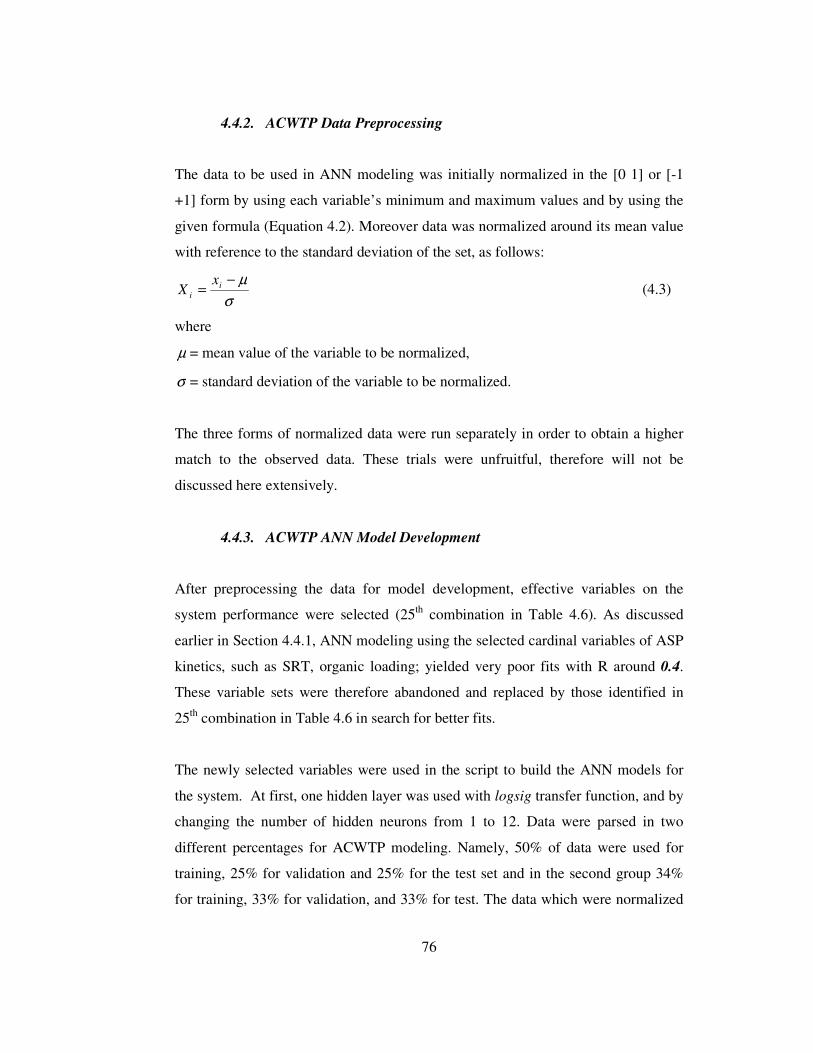
76
4.4.2. ACWTP Data Preprocessing
The data to be used in ANN modeling was initially normalized in the [0 1] or [-1
+1] form by using each variable’s minimum and maximum values and by using the
given formula (Equation 4.2). Moreover data was normalized around its mean value
with reference to the standard deviation of the set, as follows:
σµ−
= ii
xX (4.3)
where
µ = mean value of the variable to be normalized,
σ = standard deviation of the variable to be normalized.
The three forms of normalized data were run separately in order to obtain a higher
match to the observed data. These trials were unfruitful, therefore will not be
discussed here extensively.
4.4.3. ACWTP ANN Model Development
After preprocessing the data for model development, effective variables on the
system performance were selected (25th combination in Table 4.6). As discussed
earlier in Section 4.4.1, ANN modeling using the selected cardinal variables of ASP
kinetics, such as SRT, organic loading; yielded very poor fits with R around 0.4.
These variable sets were therefore abandoned and replaced by those identified in
25th combination in Table 4.6 in search for better fits.
The newly selected variables were used in the script to build the ANN models for
the system. At first, one hidden layer was used with logsig transfer function, and by
changing the number of hidden neurons from 1 to 12. Data were parsed in two
different percentages for ACWTP modeling. Namely, 50% of data were used for
training, 25% for validation and 25% for the test set and in the second group 34%
for training, 33% for validation, and 33% for test. The data which were normalized
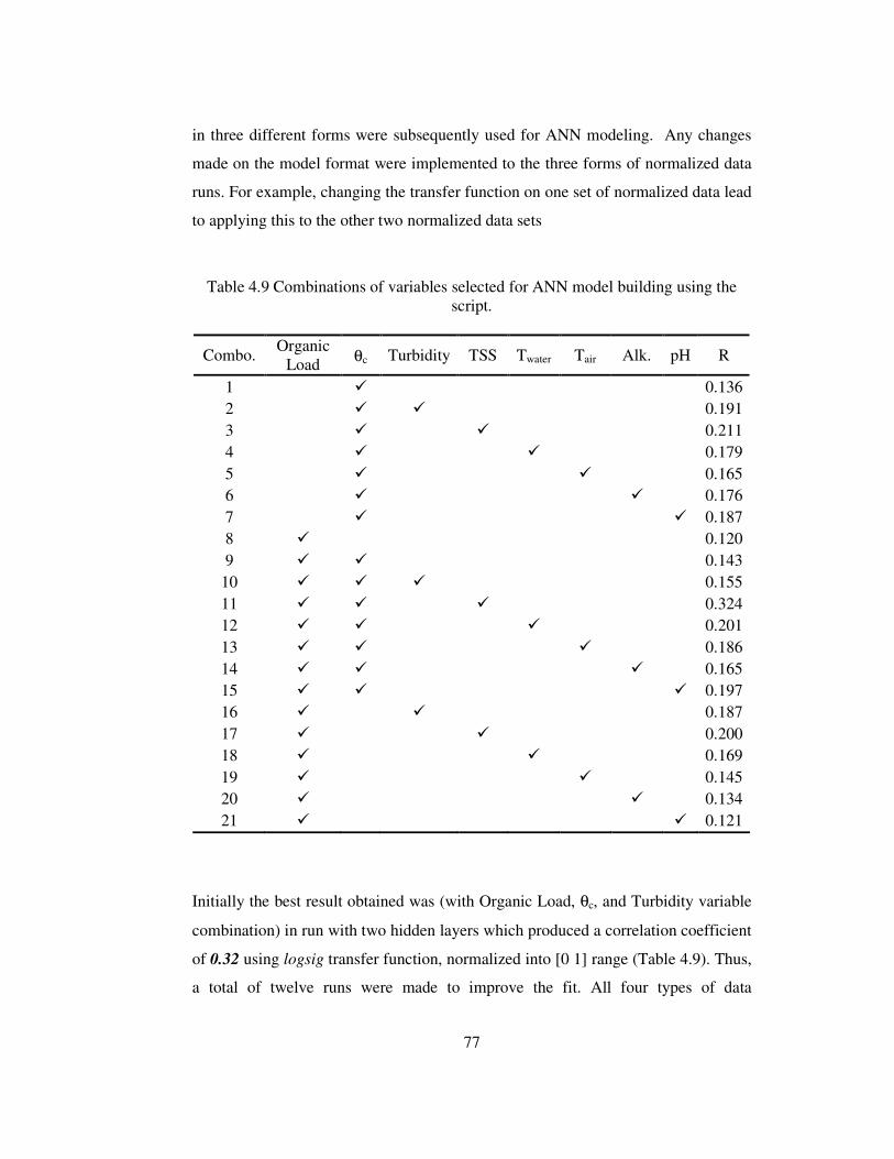
77
in three different forms were subsequently used for ANN modeling. Any changes
made on the model format were implemented to the three forms of normalized data
runs. For example, changing the transfer function on one set of normalized data lead
to applying this to the other two normalized data sets
Table 4.9 Combinations of variables selected for ANN model building using the script.
Combo. Organic Load θc Turbidity TSS Twater Tair Alk. pH R
1 0.136 2 0.191 3 0.211 4 0.179 5 0.165 6 0.176 7 0.187 8 0.120 9 0.143
10 0.155 11 0.324 12 0.201 13 0.186 14 0.165 15 0.197 16 0.187 17 0.200 18 0.169 19 0.145 20 0.134 21 0.121
Initially the best result obtained was (with Organic Load, θc, and Turbidity variable
combination) in run with two hidden layers which produced a correlation coefficient
of 0.32 using logsig transfer function, normalized into [0 1] range (Table 4.9). Thus,
a total of twelve runs were made to improve the fit. All four types of data
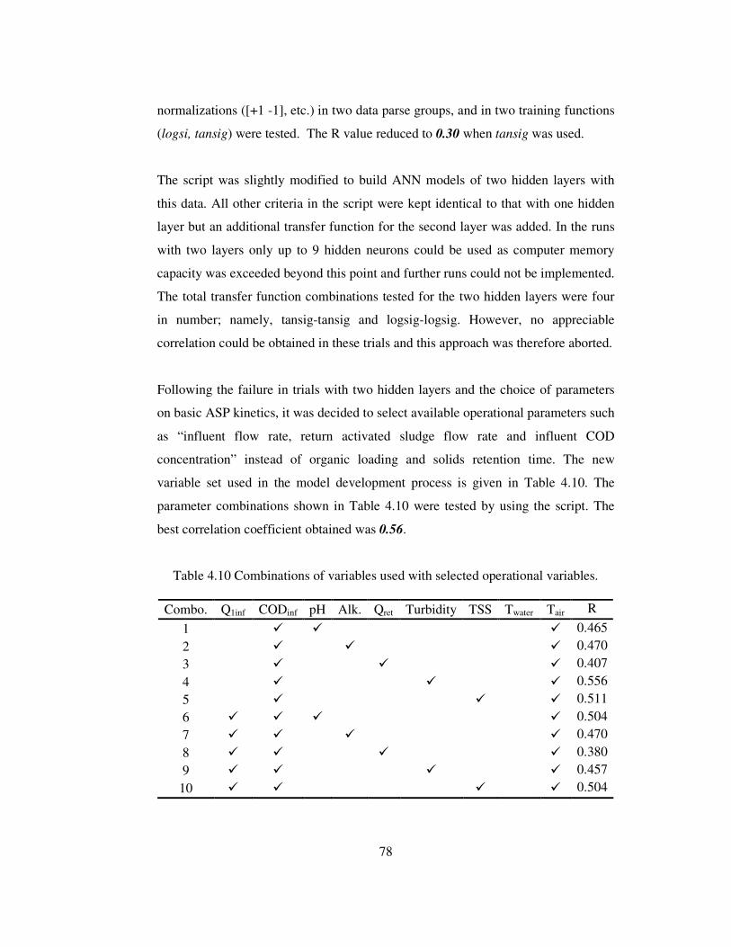
78
normalizations ([+1 -1], etc.) in two data parse groups, and in two training functions
(logsi, tansig) were tested. The R value reduced to 0.30 when tansig was used.
The script was slightly modified to build ANN models of two hidden layers with
this data. All other criteria in the script were kept identical to that with one hidden
layer but an additional transfer function for the second layer was added. In the runs
with two layers only up to 9 hidden neurons could be used as computer memory
capacity was exceeded beyond this point and further runs could not be implemented.
The total transfer function combinations tested for the two hidden layers were four
in number; namely, tansig-tansig and logsig-logsig. However, no appreciable
correlation could be obtained in these trials and this approach was therefore aborted.
Following the failure in trials with two hidden layers and the choice of parameters
on basic ASP kinetics, it was decided to select available operational parameters such
as “influent flow rate, return activated sludge flow rate and influent COD
concentration” instead of organic loading and solids retention time. The new
variable set used in the model development process is given in Table 4.10. The
parameter combinations shown in Table 4.10 were tested by using the script. The
best correlation coefficient obtained was 0.56.
Table 4.10 Combinations of variables used with selected operational variables.
Combo. Q1inf CODinf pH Alk. Qret Turbidity TSS Twater Tair R
1 0.465 2 0.470 3 0.407 4 0.556 5 0.511 6 0.504 7 0.470 8 0.380 9 0.457
10 0.504

79
The poor fit with R=0.56 suggested that other remaining variable combinations also
be tested. In order to implicate the correct variables for ANN combinations a
regression analyses between the possible input variables and the outputs (COD) was
carried out. The resultant correlation matrix is given in Table 4.12 and combinations
of selected variables after regression analysis are given in Table 4.11.
Table 4.11 Combinations of variables determined with the regression analysis used
in the individual runs of the script.
Combo. CODeffprimarysed TSSeff Tair Twater 1
2
3
4
The best correlation coefficient obtained with these variable combinations in Table
4.11 was 0.688 (from Combo. 1) which corresponded to the best result obtained for
ACWTP in all the models developed. Graphical outputs for model predictions,
regression analysis, and training session are given in Figures 4.27, 4.28, 4.29.
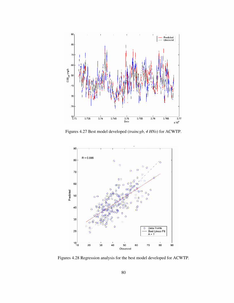
80
Figures 4.27 Best model developed (traincgb, 4 HNs) for ACWTP.
Figures 4.28 Regression analysis for the best model developed for ACWTP.

81
CO
Def
f
1.00
0
Alk
alin
ity
1.00
0
0.12
9
pH
1.00
0
0.19
8
0.04
8
T su
1.00
0
-0.5
85
-0.4
90
-0.0
44
TSS
1.00
0
0.23
2
-0.3
17
-0.0
92
0.04
8
Turb
idity
1.00
0
0.52
9
0.29
8
-0.3
17
-0.2
20
0.07
5
Qre
t
1.00
0
-0.2
01
-0.3
01
-0.5
67
0.39
4
0.03
1
-0.1
52
θ cr1
1.00
0
0.49
4
-0.1
07
-0.1
78
-0.6
37
0.33
5
0.34
7
-0.0
70
CO
Din
f
1.00
0
-0.0
92
-0.2
74
0.38
3
0.46
3
0.13
5
-0.3
31
0.13
7
0.31
0
Q1i
nf
1.00
0
-0.2
28
0.17
7
0.42
8
-0.0
04
-0.2
23
-0.3
75
0.29
3
-0.1
88
-0.0
18
Tab
le 4
.12
Var
iabl
e C
orre
latio
n m
atri
x.
Q1i
nf
CO
Din
f
θ cr1
Qre
t
Turb
idity
TSS
T su
pH
Alk
alin
ity
CO
Def
f
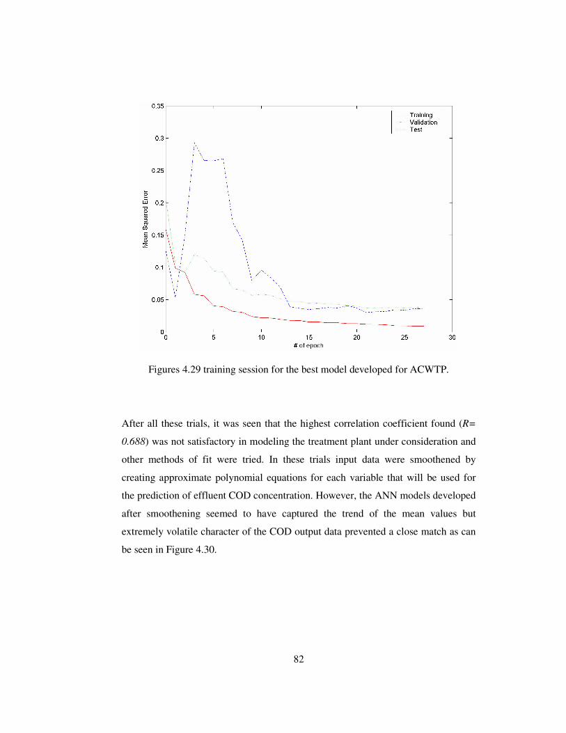
82
Figures 4.29 training session for the best model developed for ACWTP.
After all these trials, it was seen that the highest correlation coefficient found (R=
0.688) was not satisfactory in modeling the treatment plant under consideration and
other methods of fit were tried. In these trials input data were smoothened by
creating approximate polynomial equations for each variable that will be used for
the prediction of effluent COD concentration. However, the ANN models developed
after smoothening seemed to have captured the trend of the mean values but
extremely volatile character of the COD output data prevented a close match as can
be seen in Figure 4.30.

83
Figures 4.30 Prediction with polynomial data using two hidden layers for ACWTP.
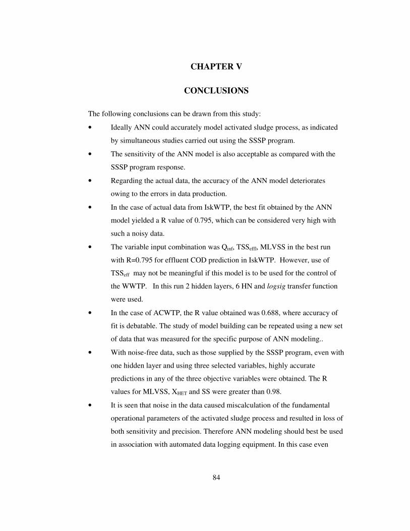
84
CHAPTER V
5. CONCLUSIONS
The following conclusions can be drawn from this study:
• Ideally ANN could accurately model activated sludge process, as indicated
by simultaneous studies carried out using the SSSP program.
• The sensitivity of the ANN model is also acceptable as compared with the
SSSP program response.
• Regarding the actual data, the accuracy of the ANN model deteriorates
owing to the errors in data production.
• In the case of actual data from IskWTP, the best fit obtained by the ANN
model yielded a R value of 0.795, which can be considered very high with
such a noisy data.
• The variable input combination was Qinf, TSSeffl, MLVSS in the best run
with R=0.795 for effluent COD prediction in IskWTP. However, use of
TSSeff may not be meaningful if this model is to be used for the control of
the WWTP. In this run 2 hidden layers, 6 HN and logsig transfer function
were used.
• In the case of ACWTP, the R value obtained was 0.688, where accuracy of
fit is debatable. The study of model building can be repeated using a new set
of data that was measured for the specific purpose of ANN modeling..
• With noise-free data, such as those supplied by the SSSP program, even with
one hidden layer and using three selected variables, highly accurate
predictions in any of the three objective variables were obtained. The R
values for MLVSS, XHET and SS were greater than 0.98.
• It is seen that noise in the data caused miscalculation of the fundamental
operational parameters of the activated sludge process and resulted in loss of
both sensitivity and precision. Therefore ANN modeling should best be used
in association with automated data logging equipment. In this case even

85
systematic bias that would be produced by the instrumentation would not
appreciably impact the precision of the predictions. Whereas manual data
produced may contain both random and systematic errors which result in
great loss of precision.
86
REFERENCES
Albiol, J., Campmajo, C., Casas, C., Poch, M. “Biomass Estimation in Plant Cell
Cultures: a Neural Network Approach.” Biotechnology Progress 11 (1995): 88–92.
Baran, P., Lek, S., Delacoste, M., Belaud, A. “Stochastic Models that Predict Trouts
Population Densities or Biomass on Macrohabitat Scale.” Hydrobiologia 337
(1996): 1–9.
Brey, T., Jarre-Teichmann, A., Borlich, O. “Artificial Neural Network versus
Multiple Linear Regression: Predicting P:B Ratios from Empirical Data.” Marine
Ecology Progress Series 140 (1996): 251–256.
Chitra, S.P. “Use Neural Networks for Problem Solving.” Chemical Enginerring
Progress (1993): 44-52.
Choi, D., Park, H. “A Hybrid Artificial Neural Network as a Software Sensor for
Optimal Control of a Wastewater Treatment Process.” Water Research 35.16
(2001): 3959-3967.
Colasanti, R.L. “Discussions of the Possible Use of Neural Network Algorithms in
Ecological Modelling.” Binary 3 (1991): 13–15.
Côte, M., Grandjean, B.P.A., Lessard, P., Thibault, J. “Dynamic Modelling of the
Activated Sludge Process: Improving Prediction using Neural Networks.” Water
Research 29.4 (1995): 995-1004.

87
Edwards, M., Morse, D.R. “The Potential for Computer-aided Identification in
Biodiversity Research.” Trends in Ecology & Evolution 10 (1995): 153–158.
Faraggi, D., Simon, R. “A Neural Network Model for Survival Data.” Statistics in
Medicine 14 (1995): 73–82.
Fausett, L. “Fundamentals of Neural Networks, Architectures, Algorithms, and
Applications.” 1994.
Gernaey, K.V., van Loosdrecht, M.C.M., Henze, M., Lind, M., Jrgensen, S.B.
“Activated Sludge wastewater treatment plant modelling and simulation: state of the
art.”, Environmental Modelling & Software 19 (2004): 763-783.
Giske, J., Huse, G., Fiksen, O. “Modelling Spatial Dynamics of Fish.” Reviews in
Fish and Biology Fisheries 8 (1998): 57–91.
Gontarski, C.A., Rodrigues, P.R., Mori, M., Prenem, L.F. “Simulation of an
Industrial Wastewater Treatment Plant using Artificial Neural Networks.”
Computers and Chemical Engineering 24 (2000): 1719-1723.
Gujer, W., Henze, M., Mino, T., Loosdrecht, M. V. “Activated Sludge Model No.
3.” Water Science and Technology 39.1 (1999): 183–193
Hamed, M. M., Khalafallah, M. G., Hassanien E. A. “Prediction of wastewater
treatment plant performance using artificial neural networks” Environmental
Modelling & Software (19) 2004: 919-928.
Hecht-Nielsen, R. “Kolmogorov’s Mapping Neural Network Existence Theorem.”
Proceedings of the First IEEE International Joint Conference on Neural Networks,
New York, (1987): 11–14.
88
Henze, M., Gujer, W., Mino, T., Matsuo, T., Wentzel, M.C., Marais, G.V.R.
"Wastewater and Biomass Characterization for the Activated Sludge Model No. 2:
Biological Phosphorus Removal." Water Science and Technology (1995): 13-23.
Henze, M., Leslie Grady, C.P., Gujer Jr, W., Marais, G.V.R., Matsuo, T. "A General
Model For Single-Sludge Wastewater Treatment Systems." Water Research (1987):
505-515.
Jain, A.K., Mao, J. “Artificial Neural Networks: A Tutorial.” Computer (1996): 31-
44.
Kastens, T.L., Featherstone, A.M. “Feedforward Backpropagation Neural Networks
in Prediction of Farmer Risk Preference.” American Journal of Agricultural
Economics 78 (1996): 400–415.
Keller, P.E., Kouzes, R.T., Kangas, L.J. “Three Neural Network Based Sensor
Systems for Environmental Monitoring.” IEEE Electro International Conference,
Boston 1994.
Konar, A. “Artificial Intelligence and Soft Computing, Behavioral and Cognitive
Modeling of the Human Brain.” 1999.
Lek, S., Delacoste, M., Baran, P., Dimopoulos, I., Lauga, J., Aulagnier, S.
“Application of Neural Networks to Modelling Nonlinear Relationships in
Ecology.” Ecological Modelling 90 (1996): 39-52.
Lek., S., Guègan, J.F. “Artificial Neural Networks as a Tool in Ecological
Modelling, an Introduction.” Ecological Modelling 120 (1999): 65-73.

89
Lerner, B., Levinstein, M., Rosenberg, B., Guterman, H., Dinstein, I., Romem, Y.
“Feature Selection and Chromosomes Classification using a Multilayer Perceptron
Neural Network.” IEEE Int. Confer. on Neural Networks, Florida (1994): 3540–
3545.
Lo, J.Y., Baker, J.A., Kornguth, P.J., Floyd, C.E. “Application of Artificial Neural
Networks to Interpretation of Mammograms on the Basis of the Radiologists
Impression and Optimized Image Features.” Radiology 197 (1995): 242–242.
Lobbrecht, A.H., Solomatine, D.P. “Machine Learning in Real Time Control of
Water Systems.” Urban Water 4 (2002): 283-289.
Maier, H.R., Dandy, G.C. “Neural Network Based Modelling of Environmental
Variables: a Systematic Approach.” Mathematical and Computer Modelling 33.6-7
(2001):669-682.
Masson, M.H., Canu, S., Grandvalet, Y., Lynggaard-Jensen, A. “Software Sensor
Design Basen on Empirical Data.” Ecological Modelling 120 (1999): 131-139.
Morshed, J., Kaluarachchi, J.J. “Application of Artificial Neural Network and
Genetic Algorithm in Flow and Transport Simulations.” Advances in Water
Resources 22.2 (1998): 45-158.
Murtagh, F., Zheng, G., Chambell, J.G., Aussem, A. “Neural Network Modelling
for Environmental Prediction.” Neurocomputing 30 (2000): 65-70.
Recknagel, F., French, M., Harkonen, P., Yabunaka, K.I. “Artificial Neural Network
Approach for Modelling and Prediction of Algal Blooms.” Ecological Modelling 96
(1997): 11–28.
90
Roger, L.L., Dowla, F.U. “Optimization of Groundwater Remediation using
Artificial Neural Networks with Parallel Solute Transport Modelling.” Water
Resources Research 30.2 (1994): 457-481.
Rodriguez, M.J., Sérodes, J.B. “Assessing Empirical Linear and Non-linear
Modelling of Residual Chlorine in Urban Drinking Water Systems.” Environmental
Modelling & Software 14 (1999): 93-102.
Scardi, M. “Artificial Neural Networks as Empirical Models for Estimating
Phytoplankton Production.” Marine Ecology Progress Series 139 (1996): 289–299.
Seginer, I., Boulard, T., Bailey, B.J. “Neural Network Models of the Greenhouse
Climate.” Journal of Agricultural Engineering Research 59 (1994): 203–216.
Sin, G. “Determination of ASM1 Sensitive Parameters and Simulation Studies for
Ankara Wastewater Treatment Plant.” M.S. Thesis, METU 2000.
Tchobanoglous, G., Burton, F. L. “Wastewater Engineering: Treatment, Disposal
and Reuse.” McGraw-Hill Series in Water Resources and Environmental
Engineering, 1991.
Zeng, G.M., Qin, X.S., He, L., Huang, G.H., Liu, H.L., Lin, Y.P. “A neural
network predictive control system for paper mill wastewater treatment” Artificial
Intelligence (16) 2003: 121-129.
Zilouchian, A., Jamshidi, M. “Intelligent Control Systems Using Soft Computing
Methodologies.” 2001.

91
APPENDICES
APPENDIX A
SSSP Simulation Program Default Dynamic Data Figures & Tables
A.1. SSSP Simulation Program Default Influent Data
Table A.1. Input Data given in the SSSP Program.
Input Normalized Input Time Flow Xi Sol. Org. Flow Xi Sol. Org. 0 725 30.1 98.9 0.27281 0.45477 0.45441 1 594 27.7 91.0 0.15447 0.39447 0.39387 2 524 21.7 71.2 0.09124 0.24372 0.24215 3 453 19.2 63.2 0.02710 0.18090 0.18084 4 423 16.9 55.4 0.00000 0.12312 0.12107 5 423 15.6 51.4 0.00000 0.09045 0.09042 6 503 13.2 43.5 0.07227 0.03015 0.02989 7 725 12.0 39.6 0.27281 0.00000 0.00000 8 1128 12.0 39.6 0.63686 0.00000 0.00000 9 1409 15.6 51.4 0.89070 0.09045 0.09042 10 1460 24.1 79.1 0.93677 0.30402 0.30268 11 1440 36.7 120.6 0.91870 0.62060 0.62069 12 1470 43.3 142.4 0.94580 0.78643 0.78774 13 1530 48.2 158.2 1.00000 0.90955 0.90881 14 1510 48.8 160.2 0.98193 0.92462 0.92414 15 1420 48.2 158.2 0.90063 0.90955 0.90881 16 1329 51.8 170.1 0.81843 1.00000 1.00000 17 1208 51.2 168.1 0.70912 0.98492 0.98467 18 1097 48.2 158.2 0.60885 0.90955 0.90881 19 1027 41.5 136.4 0.54562 0.74121 0.74176 20 1007 36.1 118.7 0.52755 0.60553 0.60613 21 926 34.3 112.7 0.45438 0.56030 0.56015 22 886 33.7 110.8 0.41825 0.54523 0.54559 23 785 32.5 106.8 0.32701 0.51508 0.51494 Min 423 12.0 39.6 0.00000 0.00000 0.00000 Max 1530 51.8 170.1 1.00000 1.00000 1.00000
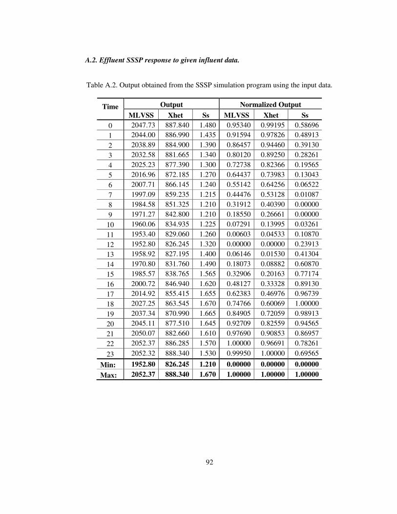
92
A.2. Effluent SSSP response to given influent data.
Table A.2. Output obtained from the SSSP simulation program using the input data.
Output Normalized Output Time MLVSS Xhet Ss MLVSS Xhet Ss
0 2047.73 887.840 1.480 0.95340 0.99195 0.58696 1 2044.00 886.990 1.435 0.91594 0.97826 0.48913 2 2038.89 884.900 1.390 0.86457 0.94460 0.39130 3 2032.58 881.665 1.340 0.80120 0.89250 0.28261 4 2025.23 877.390 1.300 0.72738 0.82366 0.19565 5 2016.96 872.185 1.270 0.64437 0.73983 0.13043 6 2007.71 866.145 1.240 0.55142 0.64256 0.06522 7 1997.09 859.235 1.215 0.44476 0.53128 0.01087 8 1984.58 851.325 1.210 0.31912 0.40390 0.00000 9 1971.27 842.800 1.210 0.18550 0.26661 0.00000
10 1960.06 834.935 1.225 0.07291 0.13995 0.03261 11 1953.40 829.060 1.260 0.00603 0.04533 0.10870 12 1952.80 826.245 1.320 0.00000 0.00000 0.23913 13 1958.92 827.195 1.400 0.06146 0.01530 0.41304 14 1970.80 831.760 1.490 0.18073 0.08882 0.60870 15 1985.57 838.765 1.565 0.32906 0.20163 0.77174 16 2000.72 846.940 1.620 0.48127 0.33328 0.89130 17 2014.92 855.415 1.655 0.62383 0.46976 0.96739 18 2027.25 863.545 1.670 0.74766 0.60069 1.00000 19 2037.34 870.990 1.665 0.84905 0.72059 0.98913 20 2045.11 877.510 1.645 0.92709 0.82559 0.94565 21 2050.07 882.660 1.610 0.97690 0.90853 0.86957 22 2052.37 886.285 1.570 1.00000 0.96691 0.78261
23 2052.32 888.340 1.530 0.99950 1.00000 0.69565
Min: 1952.80 826.245 1.210 0.00000 0.00000 0.00000 Max: 2052.37 888.340 1.670 1.00000 1.00000 1.00000
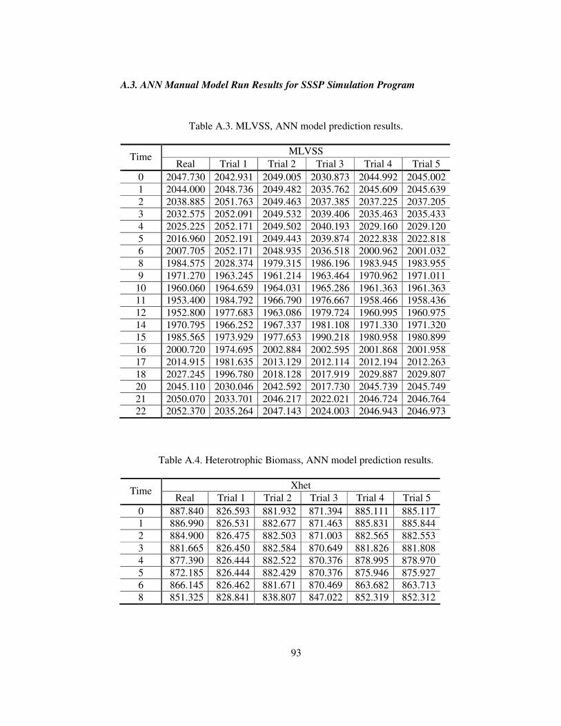
93
A.3. ANN Manual Model Run Results for SSSP Simulation Program
Table A.3. MLVSS, ANN model prediction results.
MLVSS Time Real Trial 1 Trial 2 Trial 3 Trial 4 Trial 5
0 2047.730 2042.931 2049.005 2030.873 2044.992 2045.002 1 2044.000 2048.736 2049.482 2035.762 2045.609 2045.639 2 2038.885 2051.763 2049.463 2037.385 2037.225 2037.205 3 2032.575 2052.091 2049.532 2039.406 2035.463 2035.433 4 2025.225 2052.171 2049.502 2040.193 2029.160 2029.120 5 2016.960 2052.191 2049.443 2039.874 2022.838 2022.818 6 2007.705 2052.171 2048.935 2036.518 2000.962 2001.032 8 1984.575 2028.374 1979.315 1986.196 1983.945 1983.955 9 1971.270 1963.245 1961.214 1963.464 1970.962 1971.011
10 1960.060 1964.659 1964.031 1965.286 1961.363 1961.363 11 1953.400 1984.792 1966.790 1976.667 1958.466 1958.436 12 1952.800 1977.683 1963.086 1979.724 1960.995 1960.975 14 1970.795 1966.252 1967.337 1981.108 1971.330 1971.320 15 1985.565 1973.929 1977.653 1990.218 1980.958 1980.899 16 2000.720 1974.695 2002.884 2002.595 2001.868 2001.958 17 2014.915 1981.635 2013.129 2012.114 2012.194 2012.263 18 2027.245 1996.780 2018.128 2017.919 2029.887 2029.807 20 2045.110 2030.046 2042.592 2017.730 2045.739 2045.749 21 2050.070 2033.701 2046.217 2022.021 2046.724 2046.764 22 2052.370 2035.264 2047.143 2024.003 2046.943 2046.973
Table A.4. Heterotrophic Biomass, ANN model prediction results.
Xhet Time Real Trial 1 Trial 2 Trial 3 Trial 4 Trial 5
0 887.840 826.593 881.932 871.394 885.111 885.117 1 886.990 826.531 882.677 871.463 885.831 885.844 2 884.900 826.475 882.503 871.003 882.565 882.553 3 881.665 826.450 882.584 870.649 881.826 881.808 4 877.390 826.444 882.522 870.376 878.995 878.970 5 872.185 826.444 882.429 870.376 875.946 875.927 6 866.145 826.462 881.671 870.469 863.682 863.713 8 851.325 828.841 838.807 847.022 852.319 852.312

94
Table A.4.(continued).
9 842.800 836.186 831.057 831.728 843.420 843.439 10 834.935 833.237 832.051 833.094 831.386 831.355 11 829.060 829.362 830.995 841.899 827.903 827.884 12 826.245 834.286 829.443 844.793 828.940 828.928 14 831.760 852.039 832.007 846.575 833.212 833.181 15 838.765 843.663 835.944 853.244 837.360 837.310 16 846.940 848.655 853.877 862.043 848.487 848.506 17 855.415 842.930 860.664 867.203 853.952 853.995 18 863.545 833.243 860.782 869.469 863.986 863.986 20 877.510 826.816 872.984 868.196 878.535 878.504 21 882.660 826.717 877.790 869.656 882.435 882.435 22 886.285 826.686 879.131 870.233 883.615 883.621
Table A.5. Suspended Solids, ANN model prediction results.
Ss Time Real Trial 1 Trial 2 Trial 3 Trial 4 Trial 5
0 1.480 1.226 1.670 1.511 1.483 1.483 1 1.435 1.221 1.670 1.519 1.481 1.481 2 1.390 1.215 1.670 1.519 1.349 1.349 3 1.340 1.214 1.670 1.521 1.332 1.332 4 1.300 1.213 1.670 1.521 1.292 1.292 5 1.270 1.213 1.670 1.520 1.268 1.268 6 1.240 1.213 1.670 1.514 1.229 1.229 8 1.210 1.216 1.670 1.334 1.218 1.218 9 1.210 1.219 1.670 1.245 1.216 1.216
10 1.225 1.222 1.670 1.252 1.224 1.224 11 1.260 1.236 1.669 1.300 1.273 1.273 12 1.320 1.348 1.666 1.314 1.342 1.342 14 1.490 1.589 1.657 1.320 1.486 1.487 15 1.565 1.567 1.661 1.362 1.550 1.550 16 1.620 1.630 1.644 1.420 1.624 1.624 17 1.655 1.619 1.645 1.461 1.637 1.637 18 1.670 1.527 1.660 1.483 1.649 1.649 20 1.645 1.235 1.670 1.476 1.627 1.626 21 1.610 1.232 1.670 1.489 1.600 1.600 22 1.570 1.231 1.670 1.495 1.586 1.587
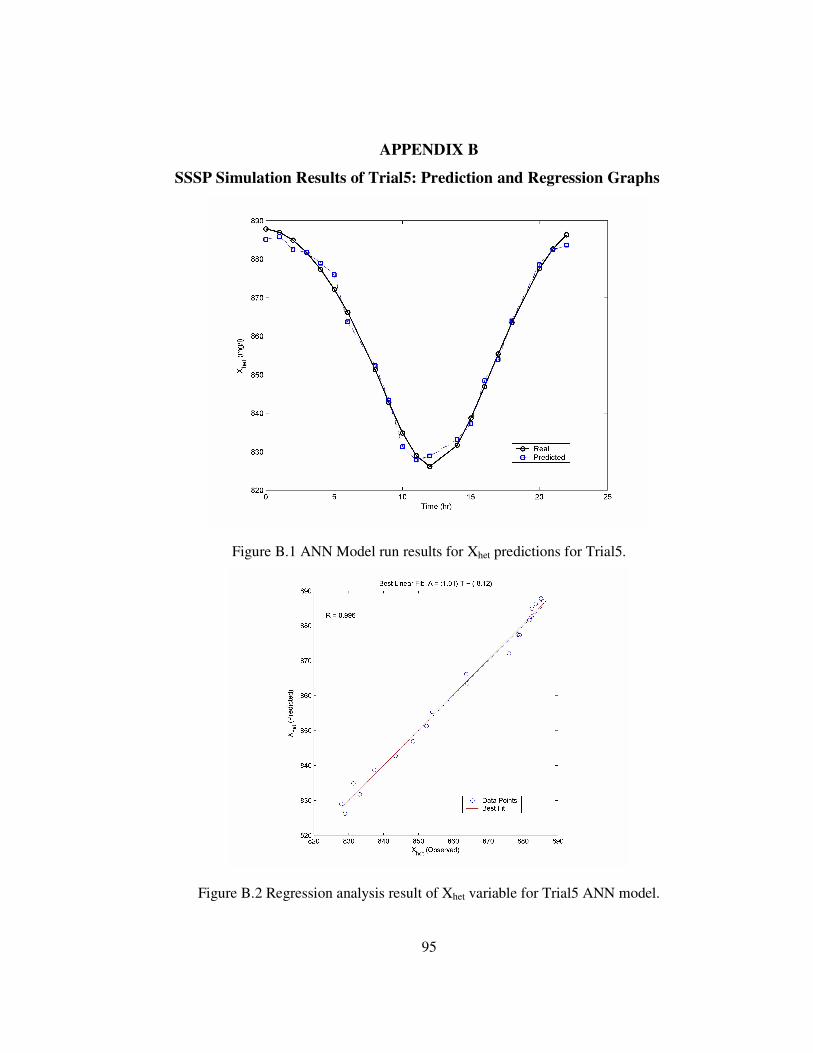
95
APPENDIX B
SSSP Simulation Results of Trial5: Prediction and Regression Graphs
Figure B.1 ANN Model run results for Xhet predictions for Trial5.
Figure B.2 Regression analysis result of Xhet variable for Trial5 ANN model.
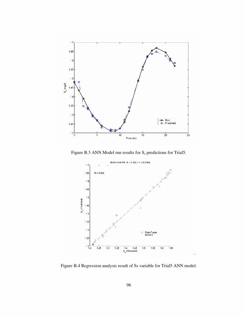
96
Figure B.3 ANN Model run results for Ss predictions for Trial5.
`
Figure B.4 Regression analysis result of Ss variable for Trial5 ANN model.
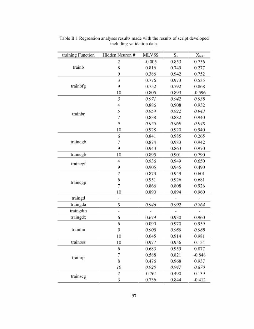
97
Table B.1 Regression analyses results made with the results of script developed including validation data.
training Function Hidden Neuron # MLVSS Ss Xhet
2 -0.005 0.853 0.756 8 0.816 0.749 0.277 trainb 9 0.386 0.942 0.752 3 0.776 0.973 0.535 9 0.752 0.792 0.868 trainbfg 10 0.805 0.893 -0.596 3 0.971 0.942 0.938 4 0.886 0.908 0.932 5 0.954 0.922 0.943 7 0.838 0.882 0.940 9 0.955 0.969 0.948
trainbr
10 0.928 0.920 0.940 6 0.841 0.985 0.265 7 0.874 0.983 0.942 traincgb 9 0.943 0.863 0.970
traıncgb 10 0.895 0.901 0.790 4 0.936 0.949 0.650 traincgf 9 0.905 0.945 0.490 2 0.873 0.949 0.601 6 0.951 0.926 0.681 7 0.866 0.808 0.926
traincgp
10 0.890 0.894 0.960 traingd - - - - traingda 8 0.946 0.992 0.864 traingdm - - - - traingdx 6 0.679 0.930 0.960
6 0.090 0.970 0.959 9 0.908 0.989 0.988 trainlm 10 0.645 0.914 0.981
trainoss 10 0.977 0.956 0.154 6 0.683 0.959 0.877 7 0.588 0.821 -0.848 8 0.476 0.968 0.937
trainrp
10 0.920 0.947 0.870 2 -0.764 0.490 0.139 trainscg 3 0.736 0.844 -0.412

98
Table B.1 (Continued).
4 0.511 0.238 -0.470 trainscg 5 0.925 0.697 -0.079 7 0.753 0.959 0.553 9 0.698 0.892 0.718 trainscg 10 0.606 0.790 0.854
Table B.2 Regression analyses results using the script developed discarding validation data.
Training Function Hidden Neuron # MLVSS Ss Xhet
5 0.932 0.910 0.911 6 0.928 0.881 0.958 9 0.860 0.971 0.964
trainb
10 0.987 0.928 0.950 3 0.985 0.993 943.000 4 0.985 0.964 0.977 5 0.992 0.988 0.998
trainbfg
6 0.988 0.967 0.950 8 0.990 0.988 0.928
trainbfg 10 0.986 0.965 0.978 2 0.982 0.992 0.937 3 0.988 0.992 0.946 4 0.992 0.993 0.982 5 0.992 0.994 0.980 6 0.993 0.994 0.992 7 0.991 0.994 0.991 8 0.996 0.990 0.995 9 0.996 0.991 0.994
trainbr
10 0.995 0.994 0.990 4 0.973 0.954 0.947 5 0.986 0.973 0.977 7 0.992 0.991 0.963 8 0.989 0.972 0.997 9 0.980 0.966 0.994
traincgb
10 0.998 0.987 0.995 3 0.985 0.993 0.943 4 0.985 0.993 0.943 traincgf 5 0.992 0.976 0.993
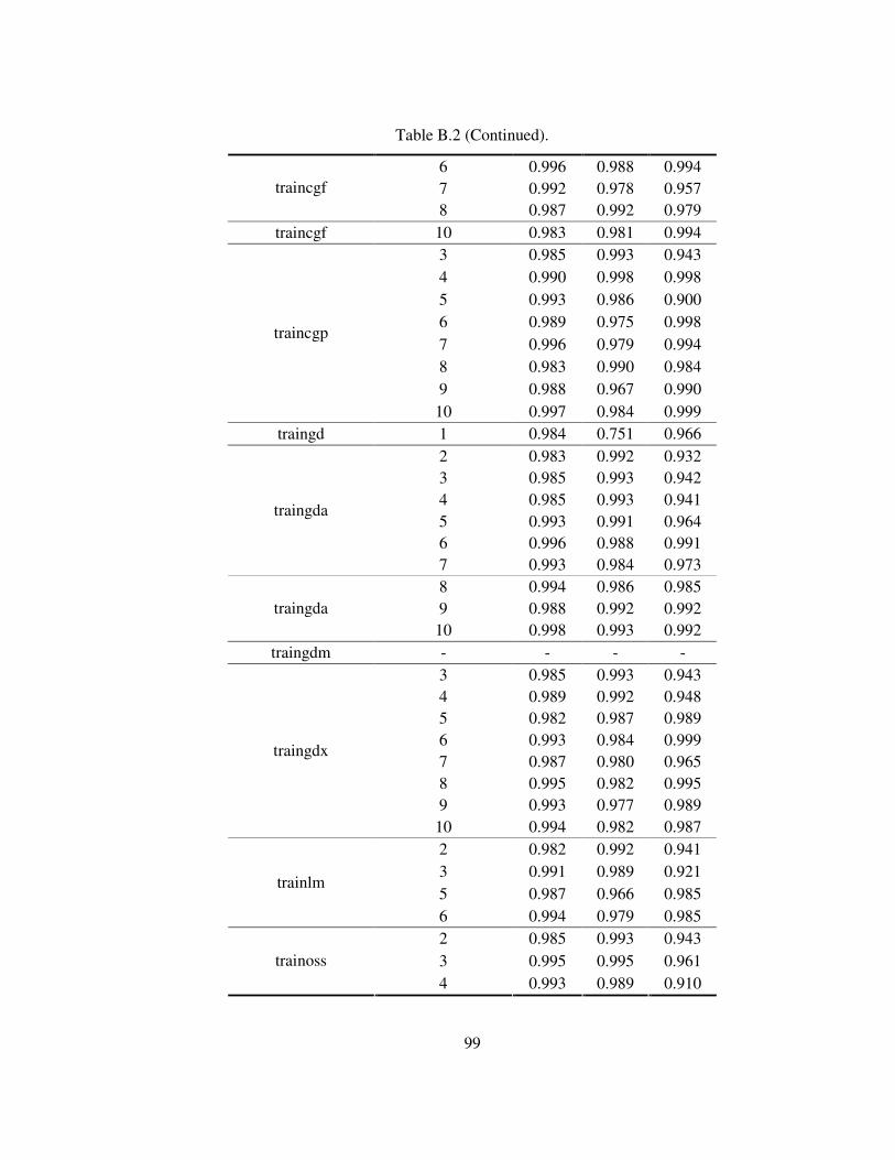
99
Table B.2 (Continued).
6 0.996 0.988 0.994 7 0.992 0.978 0.957 traincgf 8 0.987 0.992 0.979
traincgf 10 0.983 0.981 0.994 3 0.985 0.993 0.943 4 0.990 0.998 0.998 5 0.993 0.986 0.900 6 0.989 0.975 0.998 7 0.996 0.979 0.994 8 0.983 0.990 0.984 9 0.988 0.967 0.990
traincgp
10 0.997 0.984 0.999 traingd 1 0.984 0.751 0.966
2 0.983 0.992 0.932 3 0.985 0.993 0.942 4 0.985 0.993 0.941 5 0.993 0.991 0.964 6 0.996 0.988 0.991
traingda
7 0.993 0.984 0.973 8 0.994 0.986 0.985 9 0.988 0.992 0.992 traingda 10 0.998 0.993 0.992
traingdm - - - - 3 0.985 0.993 0.943 4 0.989 0.992 0.948 5 0.982 0.987 0.989 6 0.993 0.984 0.999 7 0.987 0.980 0.965 8 0.995 0.982 0.995 9 0.993 0.977 0.989
traingdx
10 0.994 0.982 0.987 2 0.982 0.992 0.941 3 0.991 0.989 0.921 5 0.987 0.966 0.985
trainlm
6 0.994 0.979 0.985 2 0.985 0.993 0.943 3 0.995 0.995 0.961 trainoss 4 0.993 0.989 0.910
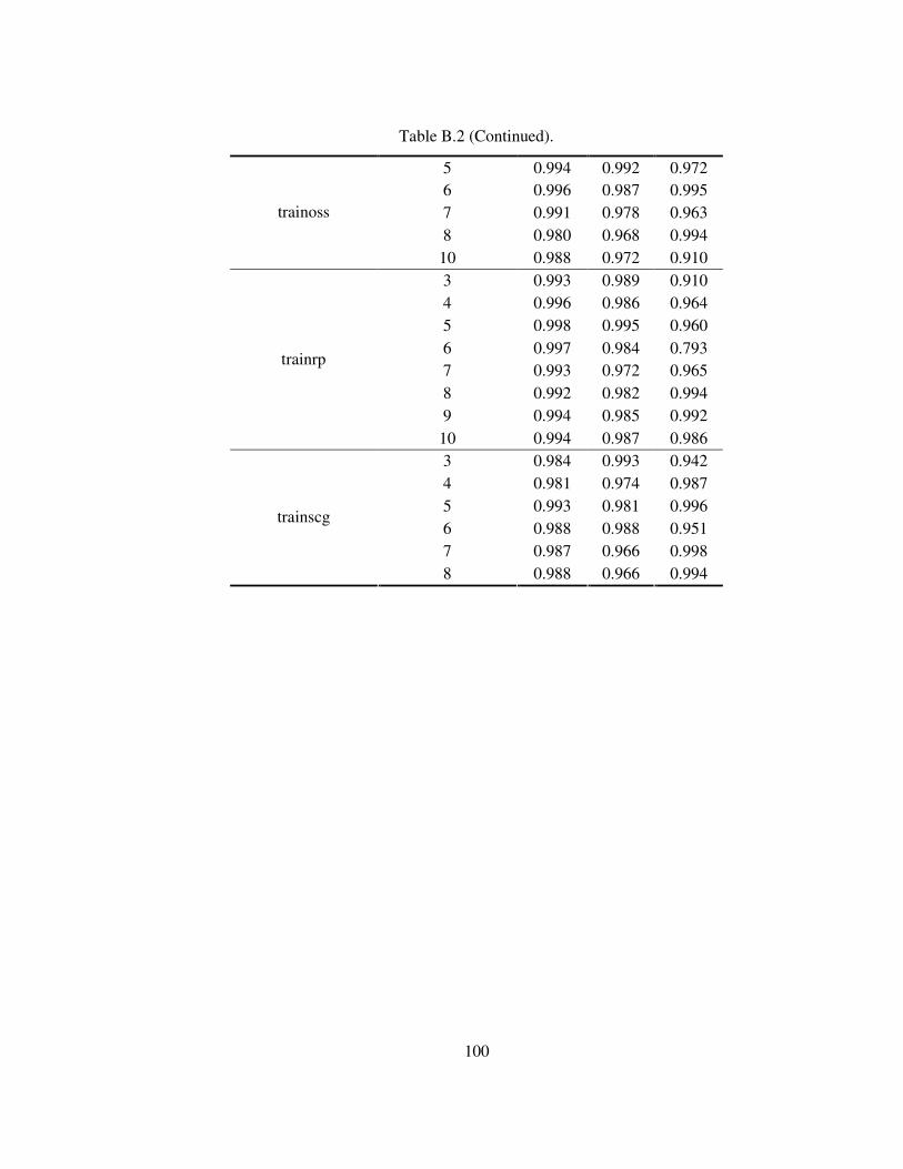
100
Table B.2 (Continued).
5 0.994 0.992 0.972 6 0.996 0.987 0.995 7 0.991 0.978 0.963 8 0.980 0.968 0.994
trainoss
10 0.988 0.972 0.910 3 0.993 0.989 0.910 4 0.996 0.986 0.964 5 0.998 0.995 0.960 6 0.997 0.984 0.793 7 0.993 0.972 0.965 8 0.992 0.982 0.994 9 0.994 0.985 0.992
trainrp
10 0.994 0.987 0.986 3 0.984 0.993 0.942 4 0.981 0.974 0.987 5 0.993 0.981 0.996 6 0.988 0.988 0.951 7 0.987 0.966 0.998
trainscg
8 0.988 0.966 0.994

101
APPENDIX C
Results of runs with IskWTP Data
Table C.1. Complete results of IskWTP run NO:25.
training function Set HNs R trainbfg 5 5 0.622 trainbfg 6 3 0.620 trainbfg 6 4 0.673 trainbfg 6 6 0.640 traincgb 5 3 0.603 traincgb 5 6 0.795 traincgb 6 4 0.616 traincgb 6 6 0.694 traincgf 5 4 0.648 traincgf 6 6 0.649 traincgp 5 5 0.664 traincgp 6 2 0.653 traingd 6 4 0.639 trainlm 6 1 0.670 trainoss 5 3 0.628 trainscg 6 6 0.668
Table C.2. Complete results of IskWTP run NO:26.
training function Set HNs R trainb 4 2 0.696 trainb 4 6 0.658
trainbfg 4 3 0.650 trainbfg 4 5 0.648 trainbfg 5 3 0.673 trainbfg 5 5 0.653 trainbfg 5 6 0.673
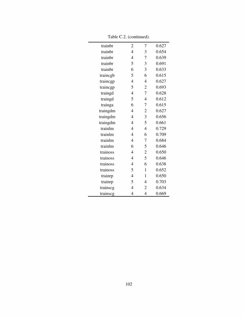
102
Table C.2. (continued).
trainbr 2 7 0.627 trainbr 4 3 0.654 trainbr 4 7 0.639 trainbr 5 3 0.691 trainbr 6 3 0.633
traincgb 5 6 0.615 traincgp 4 4 0.627 traincgp 5 2 0.693 traingd 4 7 0.628 traingd 5 4 0.612 trainga 6 7 0.615
traingdm 4 2 0.627 traingdm 4 3 0.656 traingdm 4 5 0.661 trainlm 4 4 0.729 trainlm 4 6 0.709 trainlm 4 7 0.684 trainlm 6 5 0.646 trainoss 4 2 0.650 trainoss 4 5 0.646 trainoss 4 6 0.638 trainoss 5 1 0.652 trainrp 4 1 0.650 trainrp 5 4 0.703
trainscg 4 2 0.634 trainscg 4 4 0.669

103
APPENDIX D
CODES & SCRIPTS WRITTEN
D.1. MATLAB Script Written for Automated Generation ANN Models
echo off
fortr='b' ;'bfg';'br' ;'cgb';'cgf';'cgp';'gd' ;'gda';'gdm';'gdx';'lm' ;'oss';'rp’ ;'scg';
trspaces=' ' ;'' ;' ' ;'' ;'' ;'' ;' ' ;'' ;'' ;'' ;' ' ;'' ;' ' ;'' ;
[numf1 numf2]=size(fortr);
tn=(norm01(TarAll))';
r=0;
for all=6:6 %input kombo sayisi
pn = eval(char(strcat(['(norm01(Orginp'],[num2str(all,'%02d')],['))'';'])));
[R,Q] = size(pn);
iitr = 1:floor(Q*0.50);
iival = ceil(Q*0.50):floor(0.75*Q);
iitst = ceil(0.75*Q):1:Q;
validation.P = pn(:,iival);
validation.T = tn(:,iival);
testing.P = pn(:,iitst);
testing.T = tn(:,iitst);
ptr = pn(:,iitr);
ttr = tn(:,iitr);
for y= 1:numf1
DizinYarat(y)=strcat(['mkdir(…
.\nettrain'],[fortr(y)],['_'],strcat([num2str(all,'%02d')]),[trspaces(y)],[';']);
DizinYaratti(y,:)=char(DizinYarat(y));
eval(DizinYaratti(y,:));
end
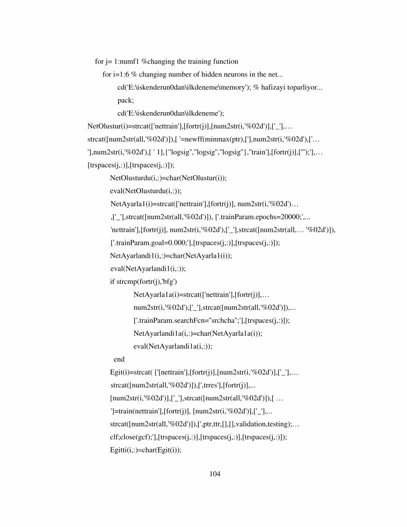
104
for j= 1:numf1 %changing the training function
for i=1:6 % changing number of hidden neurons in the net...
cd('E:\iskenderun0dan\ilkdeneme\memory'); % hafizayi toparliyor...
pack;
cd('E:\iskenderun0dan\ilkdeneme');
NetOlustur(i)=strcat(['nettrain'],[fortr(j)],[num2str(i,'%02d')],['_'],…
strcat([num2str(all,'%02d')]),[ '=newff(minmax(ptr),['],num2str(i,'%02d'),['…
'],num2str(i,'%02d'),[ ' 1],''logsig'',''logsig'',''logsig'',''train'],[fortr(j)],[''');'],…
[trspaces(j,:)],[trspaces(j,:)]);
NetOlusturdu(i,:)=char(NetOlustur(i));
eval(NetOlusturdu(i,:));
NetAyarla1(i)=strcat(['nettrain'],[fortr(j)], num2str(i,'%02d')…
,['_'],strcat([num2str(all,'%02d')]), ['.trainParam.epochs=20000;',...
'nettrain'],[fortr(j)], num2str(i,'%02d'),['_'],strcat([num2str(all,… '%02d')]),
['.trainParam.goal=0.000;'],[trspaces(j,:)],[trspaces(j,:)]);
NetAyarlandi1(i,:)=char(NetAyarla1(i));
eval(NetAyarlandi1(i,:));
if strcmp(fortr(j),'bfg')
NetAyarla1a(i)=strcat(['nettrain'],[fortr(j)],…
num2str(i,'%02d'),['_'],strcat([num2str(all,'%02d')]),...
['.trainParam.searchFcn=''srchcha'';'],[trspaces(j,:)]);
NetAyarlandi1a(i,:)=char(NetAyarla1a(i));
eval(NetAyarlandi1a(i,:));
end
Egit(i)=strcat( ['[nettrain'],[fortr(j)],[num2str(i,'%02d')],['_'],…
strcat([num2str(all,'%02d')]),[',trres'],[fortr(j)],...
[num2str(i,'%02d')],['_'],strcat([num2str(all,'%02d')]),[ …
']=train(nettrain'],[fortr(j)], [num2str(i,'%02d')],['_'],...
strcat([num2str(all,'%02d')]),[',ptr,ttr,[],[],validation,testing);…
clf;close(gcf);'],[trspaces(j,:)],[trspaces(j,:)],[trspaces(j,:)]);
Egitti(i,:)=char(Egit(i));
105
eval(Egitti(i,:));
Dene(i)=strcat(['[restrain'],[fortr(j)], num2str(i,'%02d'),['_'], …
strcat([num2str(all,'%02d')]), [']'],['=sim(nettrain' ],[fortr(j)], ...
num2str(i,'%02d'),['_'],strcat([num2str(all,'%02d')]),…
[',pn);'],['Prestrain'],[fortr(j)], num2str(i,'%02d'),['_'],...
strcat([num2str(all,'%02d')]),['= unnorm01(TarAll …
'],[',restrain'],[fortr(j)],[num2str(i,'%02d')],['_'],...
strcat([num2str(all,'%02d')]),[');'],[trspaces(j,:)],…
[trspaces(j,:)],[trspaces(j,:)],[trspaces(j,:)]);
Denedi(i,:)=char(Dene(i));
eval(Denedi(i,:));
HesaplaCizdir3(i)=strcat(['fig'],[fortr(j)], [num2str(i,'%02d')],…
['_'],strcat([num2str(all,'%02d')]),['Reg=figure;'],...
['[m'],[fortr(j)],num2str(i,'%02d'), [',b'],[fortr(j)], …
num2str(i,'%02d'),[',r'],[fortr(j)],num2str(i,'%02d'),...
[']=postreg(Prestrain'],[fortr(j)], num2str(i,'%02d'),['_'],…
strcat([num2str(all,'%02d')]),[''',TarAll'],[');'],…
['title(''Regression analysis for (train'],fortr(j),['_'],…
strcat([num2str(all,'%02d')]),[')'],['(#of HNs:'],[num2str(i,'%02d')],…
[') '');'],trspaces(j),trspaces(j),trspaces(j),trspaces(j),trspaces(j),trspaces(j));
Hesapladi3(i,:)=char(HesaplaCizdir3(i));
eval(Hesapladi3(i,:));
regresValue=eval(char(strcat(['r'],[fortr(j)],num2str(i,'%02d'))));
if regresValue>=0.40
Kaydet3(i)=strcat(['print(''-r300'',''-djpeg'',''.\nettrain'],
[fortr(j)],['_'],strcat([num2str(all,'%02d')]),...
['\fig'],[fortr(j)],num2str(i,'%02d'),['Reg''' '
);'],['close(gcf);'],trspaces(j),trspaces(j));
Kaydetti3(i,:)=char(Kaydet3(i));
eval(Kaydetti3(i,:));
HesaplaCizdir1(i)=strcat(['fig'],[fortr(j)], num2str(i,'%02d'),…

106
['_'],strcat([num2str(all,'%02d')]),['=figure; plot(trres'],…
[fortr(j)], num2str(i,'%02d'), ['_'],strcat([num2str(all,'%02d')]),...
['.epoch,trres'], [fortr(j)], num2str(i,'%02d'), ['_'],…
strcat([num2str(all,'%02d')]), ['.perf,''r'', trres'],[fortr(j)],…
num2str(i,'%02d'),['_'],strcat([num2str(all,'%02d')]), ...
['.epoch,trres'], [fortr(j)], num2str(i,'%02d'), ['_'],…
strcat([num2str(all,'%02d')]),['.vperf,'':g'',trres'],[fortr(j)],…
num2str(i,'%02d'),['_'],strcat([num2str(all,'%02d')]),...
['.epoch,trres'], [fortr(j)], num2str(i,'%02d'),…
['_'],strcat([num2str(all,'%02d')]),...
['.tperf,''-.b'');'],['xlabel(''# of epoch'');'],...
[trspaces(j,:)],[trspaces(j,:)],[trspaces(j,:)],[trspaces(j,:)],…
[trspaces(j,:)],[trspaces(j,:)],[trspaces(j,:)]);
Hesapladi1(i,:)=char(HesaplaCizdir1(i));
eval(Hesapladi1(i,:));
HesaplaCizdir11(i)=strcat(['title(''MSE vs # of Epochs (train'] ,…
[fortr(j)],['_'],strcat([num2str(all,'%02d')]),...
[')'],[' (# of HNs:'],num2str(i,'%02d'),[')'');'],[trspaces(j)],…
['legend(''training'',''Validation'',''Test'',0);…
ylabel(''Mean Squared Error'');']);
Hesapladi11(i,:)=char(HesaplaCizdir11(i));
eval(Hesapladi11(i,:));
Kaydet1(i)=strcat(['print(''-r300'',''-djpeg'',''.\nettrain'],…
[fortr(j)],['_'],strcat([num2str(all,'%02d')]),['\fig'],[fortr(j)], ...
num2str(i,'%02d'),['_'],strcat([num2str(all,'%02d')]),[''');…
close(gcf);'],[trspaces(j,:)],[trspaces(j,:)]);
Kaydetti1(i,:)=char(Kaydet1(i));
eval(Kaydetti1(i,:));
HesaplaCizdir2(i)=strcat(['fig'],[fortr(j)], num2str(i,'%02d'),…
['OwP'], ['=figure; plot(DATE,Prestrain'],[fortr(j)],...
107
num2str(i,'%02d'),['_'],strcat([num2str(all,'%02d')]),[',''.-r''…
'],[',DATE,TarAll,''-b'');'],...
['legend(''Predicted'',''Observed'',0); '],['ylabel(''COD_eff…
(mg/l)'');'],['xlabel(''Date'');'],...
['title(''Pred & Obs COD_eff (mg/l) vs Date w/ train '], …
[fortr(j)],['_'],strcat([num2str(all,'%02d')]), ['(# of HNs:',…
num2str(i,'%02d'),')'');'],[trspaces(j)],[trspaces(j)],[trspaces(j)]);
Hesapladi2(i,:)=char(HesaplaCizdir2(i));
eval(Hesapladi2(i,:));
Kaydet2(i)=strcat(['print(''-r300'',''-djpeg'',''.\nettrain'],…
[fortr(j)],['_'],strcat([num2str(all,'%02d')]),['\fig'],…
[fortr(j)], num2str(i,'%02d'),['OwP''' '); close(gcf);'],…
[trspaces(j)],[trspaces(j)]);
Kaydetti2(i,:)=char(Kaydet2(i));
eval(Kaydetti2(i,:));
end
Kaydet4(i)=strcat([ 'save .\nettrain'],[fortr(j)] ,['_'],…
strcat([num2str(all,'%02d')]), ['\nettrain'],[fortr(j)],…
num2str(i,'%02d'),['_'],strcat([num2str(all,'%02d')]),… [' net* …
Prestrain* restrain* trres*'],[' m'],fortr(j),['*'],[' b'],fortr(j),...
['* r'],fortr(j),['*'],[';close(gcf);'],['clear net* Prestrain* restrain*…
trres* fig* m'],fortr(j),['* b'],fortr(j), ['* r'],fortr(j),['*'],…
trspaces(j),trspaces(j),trspaces(j),trspaces(j),…
trspaces(j),trspaces(j),trspaces(j),trspaces(j));
Kaydetti4(i,:)=char(Kaydet4(i));
eval(Kaydetti4(i,:));
cd('E:\iskenderun0dan\ilkdeneme\memory');
pack;
cd('E:\iskenderun0dan\ilkdeneme');
end
end end
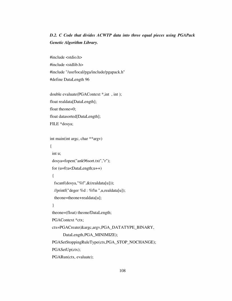
108
D.2. C Code that divides ACWTP data into three equal pieces using PGAPack
Genetic Algorithm Library.
#include <stdio.h>
#include <stdlib.h>
#include "/usr/local/pga/include/pgapack.h"
#define DataLength 96
double evaluate(PGAContext *,int , int );
float realdata[DataLength];
float theone=0;
float datasorted[DataLength];
FILE *dosya;
int main(int argc, char **argv)
int u;
dosya=fopen("ank96sort.txt","r");
for (u=0;u<DataLength;u++)
fscanf(dosya,"%f",&(realdata[u]));
//printf("deger %d : %f\n ",u,realdata[u]);
theone=theone+realdata[u];
theone=(float) theone/DataLength;
PGAContext *ctx;
ctx=PGACreate(&argc,argv,PGA_DATATYPE_BINARY,
DataLength,PGA_MINIMIZE);
PGASetStoppingRuleType(ctx,PGA_STOP_NOCHANGE);
PGASetUp(ctx);
PGARun(ctx, evaluate);

109
PGADestroy(ctx);
dosya=fopen("result.txt","w");
for (u=0;u<DataLength;u++)
fprintf(dosya,"%f\n",datasorted[u]);
fclose(dosya);
return EXIT_SUCCESS;
double evaluate(PGAContext *ctx,int p, int pop)
int i,j=0,k=0,t=0;
int stringlen;
float data1=0.0f,data2=0.0f,data3=0.0f;
for(i=0;i<DataLength;i++) //sort the array
if(PGAGetBinaryAllele(ctx,p,pop,i))
datasorted[j]=realdata[i];
j++;
else
datasorted[DataLength-k-1]=realdata[i];
k++;
for (i=0;i<DataLength;i++)
if(i<(DataLength/3))
data1=data1+datasorted[i];
else if (i>=(DataLength/3) && (i<(2*DataLength/3)))
data2=data2+datasorted[i];
else if (i>=(2*DataLength/3))
data3=data3+datasorted[i];
data1=(float) (data1/((float)(DataLength/3)));

110
data2=(float) (data2/((float)(DataLength/3)));
data3=(float) (data3/((float)(DataLength/3)));
//printf("difference : %f \n",(double)(pow(theone-data1,2)+pow(theone-
// data2,2)+pow(theone-data3,2)));
return (double) (pow(theone-data1,2)+pow(theone-data2,2)+pow(theone-
data3,2));