modeling land use change in the brazilian - dpi - inpe
TRANSCRIPT

MODELING LAND USE CHANGE IN THE BRAZILIAN AMAZON: EXPLORING
INTRA-REGIONAL HETEROGENEITY
Ana Paula Dutra de Aguiar
Doctorate Thesis in Remote Sensing, advised by Dr. Gilberto Câmara
INPE São José dos Campos
2006


“Nothing is less real than realism… Details are confusing. It is only by selection, by
elimination, by emphasis that we get at the real meaning of things”.
Georgia O'Keeffe, 1922


Dedico a meus filhos,
José Guilherme e Ana Elisa.
Tudo é uma questão de saber escolher,
dar ênfase às coisas certas.
E transformar pedras e ossos em arte...


AGRADECIMENTOS
Agradeço em especial a duas pessoas: ao Gilberto, a quem eu devo muito mais do que
esse Doutorado, e que sempre confiou em mim. E a minha amiga e colega Isabel, que
com seu bom senso e serenidade tanto me ensinou e ajudou. Agradeço ao Miguel, não
apesar, mas justamente pelas nossas divergências, que me fizeram refletir e ter certeza
do caminho a seguir. Aos meus demais companheiros de grupo, Silvana, Tiago, Felix e
Luciana, pelo apoio, troca construtiva de idéias, e amizade. Que a gente continue
trabalhando junto por muito tempo! Ao Dalton, pelas sugestões e idéias. Agradeço ao
Kasper, por tudo que me ensinou. E ao Diógenes, por ter me aberto os olhos para as
coisas que deviam ser enfatizadas.
Agradeço ao Cartaxo, Lúbia e todo o pessoal da Terralib, pelo apoio no
desenvolvimento de software. Ao Simeão e ao Consórcio ZEE/Brasil pelo banco de
dados da Amazônia. À equipe do CLUE em Wageningen por ter cedido o código para
que pudéssemos adaptá-lo para a Amazônia.
Agradeço à Rede de Pesquisa GEOMA que financiou parcialmente este trabalho. E aos
colegas do GEOMA, em especial aos companheiros do Museu Goeldi, INPA e
EMBRAPA nos trabalhos de campo, pela experiência e ótimos momentos. E, como uma
pequena homenagem, agradeço às pessoas ligadas à Comissão Pastoral da Terra que
conheci na Amazônia, em especial o Manu e o Tarcísio, que tanto me impressionaram
pelo exemplo de desprendimento e dedicação aos outros.
Agradeço à Etel, e a todos os professores e coordenadores da Pós Graduação. Aos
colegas de curso (e de “infortúnio”), em especial ao Fábio e Eduardo, pelo bom humor e
companheirismo nas intermináveis listas de exercício.... Ao Cláudio, por ser tão
prestativo sempre. À Helen, Luciana, Dinha e todas as secretárias da OBT, pela ajuda e
delicadeza sempre.
Agradeço muito a meus pais pela ajuda com as crianças, e principalmente pele incentivo
e apoio incondicional sempre, mesmo quando achavam que eu estava errada... Às
minhas irmãs e cunhados, por todo o carinho e amizade (e chopes no Heinz!!!). Em

especial minha querida Cecília, que esteve tão presente mesmo tão distante. Às minhas
sobrinhas, por alegrar nossas vidas. Agradeço ao Graco, pelo apoio com as crianças
sempre que preciso. À D. Elda e Seu José pela ajuda e carinho. Aos meus amigos que
me ajudaram a atravessar os momentos difíceis, e a entender o valor de saber pedir
ajuda quando a gente precisa. Em especial, Sueli, Isabel, Tiago, Nuno e Nei. Obrigada.
E também ao Sidnei pela inestimável e alegre companhia, e pelas músicas!
A todos da DPI pelos muitos e muitos momentos de alegria, descontração e carinho.
Tenho muito orgulho de trabalhar aqui, e ser parte deste time. Agradeço também à D.
Amélia, por cuidar de nós, e finalmente, mas não menos, ao Marcelo, pelo exemplo de
vida, com certeza alegrando as festas do céu agora...

MODELAGEM DE MUDANÇA DO USO DA TERRA NA AMAZÔNIA: EXPLORANDO A HETEROGENEIDADE INTRA-REGIONAL
RESUMO
Este trabalho descreve os resultados da aplicação de um arcabouço de modelagem
dinâmica para explorar como fatores alternativos, políticas públicas e condições de
mercado influenciam o processo de ocupação da Amazônia. Trabalhos anteriores na
Amazônia enfatizaram aspectos como distância a estradas, e desconsideraram a enorme
heterogeneidade biofísica e sócio-econômica da região. A análise estatística apresentada
usa um banco de dados espacial (células de 100 x 100 km2 e 25 x 25 km2) com 40
variáveis organizadas em células de ambientais, demográficas, de estrutura agrária,
tecnológicas, e indicadores de conectividade a mercados como variáveis independentes,
e variáveis de uso e cobertura (pastagem, agricultura temporária e permanente, floresta)
como variáveis dependentes. Os fatores determinantes dos padrões de uso foram
identificados usando modelos de regressão (spatial lag e regressão linear múltipla) para
toda a região e três sub-regiões. Os resultados dos modelos de regressão demonstram
quantitativamente que a importância relativa dos fatores determinantes apresenta grande
variação na região. Modelos de regressão enfatizam fatores associados a conexão a
mercados, conexão a portos e áreas protegidas. Os modelos foram utilizados para
realizar diferentes explorações de cenários de mudança de uso até 2020. Explorações
incluem a análise da influência de diferentes fatores na dinâmica das novas fronteiras na
Amazônia, de possíveis impactos políticas públicas, e aumento e diminuição da
demanda. As principais conclusões são: (a) conexão a mercados nacionais é o fator mais
importante para capturar os padrões espaciais das novas fronteiras; (b) a interação entre
os fatores de conexão e demais fatores biofísicos e sócio-econômicos que influencia a
dinâmica intra-regional heterogênea; (c) estas diferenças levam a impactos
diferenciados de políticas públicas na região. Este trabalho reflete a importância da
exploração de cenários como uma ferramenta para auxiliar o entendimento do processo
de ocupação da Amazônia.


MODELING LAND USE CHANGE IN THE BRAZILIAN AMAZON: EXPLORING INTRA-REGIONAL HETEROGENEITY
ABSTRACT
This work describes the results of applying a dynamical LUCC modeling framework to
explore how alternative determining factors, policies and market constraints influence
the process of land occupation in Amazonia. Previous work regarding deforestation in
Amazonia has emphasized aspects such as distance to roads, and has disregarded the
region’s enormous biophysical and socio-economical heterogeneity. The statistical
analysis uses a spatially-explicit database (cells of 100 x 100 km2 and 25 x 25 km2)
with 40 environmental, demographical, agrarian structure, technological, and market
connectivity indicators as independent variables, and land-use (pasture, temporary and
permanent crops, non-used agricultural land) patterns as dependent variables. The
determinant factors of land patterns were identified regression models (spatial lag and
multiple linear regressions) at multiple spatial resolutions for the whole region and for
three sub-regions. Regression models results showed quantitatively that the relative
importance and significance of land use determining factors greatly vary across the
Amazon. Models emphasize policy-relevant factors, especially those related to
connection to national markets, connection to ports, and protected areas. The models
were used to build different exploration scenarios of land use change until 2020.
Explorations include an analysis of the influence of different factors in the new Amazon
frontiers dynamics, the possible impacts public policies, and increasing or decreasing
demand. The main conclusions drawn from the scenario explorations are: (b) connection
to national markets is the most important factor for capturing the spatial patterns of the
new Amazonian frontiers; (b) it is the interaction between connectivity and other factors
that influence the heterogeneous intra-regional dynamics; (c) these differences led to
heterogeneous impact of policies across the region. This work reflects the importance of
scenario exploration as a tool to understand the process of occupation in the Brazilian
Amazonia.


ii
SUMÁRIO
Pág.
FIGURE LIST............................................................................................................ iv
TABLE LIST ............................................................................................................. vi
ABBREVIATION LIST ...........................................................................................vii
CHAPTER 1................................................................................................................ 1
INTRODUCTION ...................................................................................................... 1 1.1 Introduction ............................................................................................................ 1 1.2 LUCC models and the Amazonia ............................................................................ 4 1.3 Thesis hypotheses and objectives ............................................................................ 8 1.4 Document structure ............................................................................................... 10
CHAPTER 2.............................................................................................................. 13
BRAZIAN AMAZONIA: REVIEW OF HUMAN OCCUPATION PROCESS AND PREVIOUS LUCC MODELING............................................................................. 13 2.1 Human occupation and new frontiers .................................................................... 13 2.1.1 Occupation history: 1950-2000........................................................................... 13 2.1.2 Government policies for Amazonia: 1995-2005.................................................. 16 2.1.3 New expansion areas and future axes of development ........................................ 17 2.2 Review of previous LUCC modeling in the Brazilian Amazonia ........................... 21 2.2.1 Land use factors statistical analyses.................................................................... 21 2.2.2 Recent projective modeling and scenario building .............................................. 24
CHAPTER 3.............................................................................................................. 31
STUDY AREA AND DATABASE CONTRUCTION............................................. 31 3.1 Study Area ............................................................................................................ 31 3.2 Land use patterns .................................................................................................. 32 3.2.1 Deforested area patterns ..................................................................................... 32 3.2.2 Agricultural land use patterns ............................................................................. 32 3.3 Potential determinant factors ................................................................................. 37 3.3.1 Accessibility to market factors ........................................................................... 41 3.3.2 Economical attractiveness factors ....................................................................... 42 3.3.3 Demographical factors ....................................................................................... 42 3.3.4 Technological factors ......................................................................................... 42 3.3.5 Agrarian Structure factors .................................................................................. 43 3.3.6 Public Policy factors........................................................................................... 43 3.3.7 Environmental factors ........................................................................................ 44

iii
CHAPTER 4.............................................................................................................. 65
SPATIAL MODELING OF LAND-USE DETERMINANTS IN THE BRAZILIAN AMAZONIA ............................................................................................................. 65 4.1 Introduction .......................................................................................................... 65 4.2 Methods ................................................................................................................ 65 4.2.1 Exploratory analysis and selection of variables................................................... 65 4.2.2 Spatial regression modeling................................................................................ 69 4.3 Results and discussion........................................................................................... 71 4.3.1 Deforestation factors in the whole Amazonia...................................................... 71 4.3.2 Comparison of deforestation determining factors across space partitions ............ 75 4.3.3 Comparison of land-use determining factors in the Arch partition ...................... 82
CHAPTER 5.............................................................................................................. 87
EXPLORING SCENARIOS OF LAND-USE CHANGE IN THE BRAZILIAN AMAZONIA ............................................................................................................. 87 5.1 Introduction .......................................................................................................... 87 5.2 Methods ................................................................................................................ 88 5.2.1 The CLUE framework and its adaptation to Amazonia ....................................... 88 5.2.2 Basic modeling decisions ................................................................................... 90 5.2.3 Statistical analysis .............................................................................................. 90 5.2.3.1 Adequacy of Linear Regression models in LUCC models................................ 90 5.2.3.2 Statistical analysis procedure........................................................................... 91 5.2.4 Allocation module modifications........................................................................ 96 5.2.5 Scenario building ............................................................................................... 97 5.2.5.1 Overview......................................................................................................... 97 5.2.5.2 Demand scenarios ........................................................................................... 99 5.2.5.3 Allocation scenarios ...................................................................................... 100 5.2.5.4 Law enforcement scenarios ........................................................................... 106 5.3 Results and discussion......................................................................................... 107 5.3.1 Exploration A – Analysis of alternative factors: accessibility............................ 109 5.3.2 Exploration B – Analysis of alternative factors: local markets .......................... 117 5.3.3 Exploration C - Policy analysis: paving and protected areas ............................. 119 5.3.4 Exploration D - Policy analysis: law enforcement............................................. 125 5.3.5 Exploration E: Alternative demand scenarios ................................................... 132
CHAPTER 6............................................................................................................ 142
CONCLUSIONS ..................................................................................................... 142 6.1 Spatial statistical analysis conclusions................................................................. 142 6.2 Dynamic modeling conclusions........................................................................... 143 6.3 Suggestions for future work ................................................................................ 144
BIBLIOGRAPHICAL REFERENCES ................................................................. 147
iv
FIGURE LIST
FIGURE 2.1 - Human occupation in 1976 and 1987 (source: IBGE). .......................... 14 FIGURE 2.2 - New frontiers and future axes of development in the Brazilian Amazonia
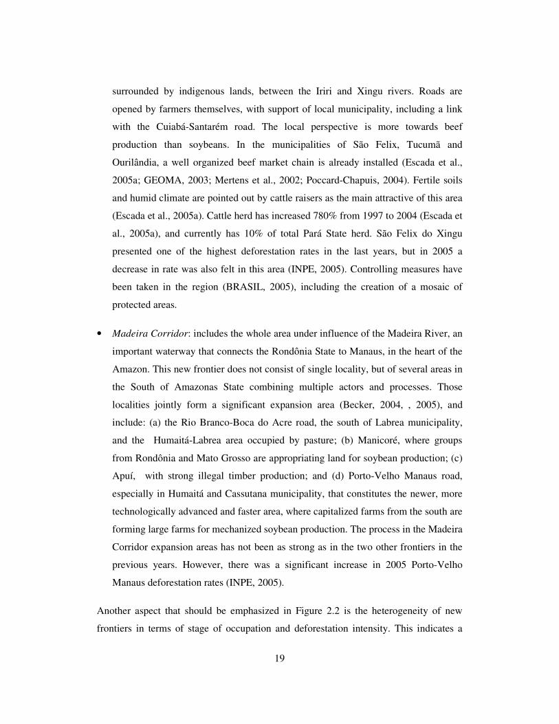
(source: adapted (Escada et al., 2005b))............................................................... 18 FIGURE 2.3 - Deforestation hot-spots in 2005 (source: (INPE, 2005)). ...................... 21 FIGURE 3.1 – Study area: (a) 25 x 25 km2; (b) 100 x 100 km2 cells. .......................... 31 FIGURE 3.2 – Deforested areas spatial pattern in 1997 (25 x 25 km2)......................... 33 FIGURE 3.3 – Pasture pattern in 1996/1997 (25 x 25 km2). ........................................ 33 FIGURE 3.4 – Temporary agriculture pattern in1996/1997 (25 x 25 km2)................... 35 FIGURE 3.5 Permanent Agriculture pattern in 1996/1997 (25 x 25 km2). ................... 35 FIGURE 3.6: Indicator of connectivity to national markets (São Paulo and Northeast) in
1997 (source of road network: IBGE).................................................................. 45 FIGURE 3.7 – Indicator of connectivity to Amazonia ports in 1997 (source of road
network: IBGE)................................................................................................... 45 FIGURE 3.8 – Distance to urban centres in 1997 (data source: IBGE). ....................... 47 FIGURE 3.9 – Distance to roads in 1997 (data source: IBGE).................................... 47 FIGURE 3.10 – Distance to paved roads in 1997 (data source: IBGE)........................ 49 FIGURE 3.11 – Distance to main rivers (data source: IBGE). .................................... 49 FIGURE 3.12 –Distance to timber production sites in 1997 (data source: MMA)....... 51 FIGURE 3.13 – Distance to mineral deposits (data source: CPRM)............................ 51 FIGURE 3.14 - Population density in 1996 (data source: IBGE Population Counting
1996)................................................................................................................... 53 FIGURE 3.15 – Technological indicator: average number of tractors per property in
1996 (data source: IBGE Agricultural Census 1996). .......................................... 55 FIGURE 3.16 - Technological indicator: percentage of farms that received technical
assistance in 1996 (data source: IBGE Agricultural Census 1996). ...................... 55 FIGURE 3.17 – Agrarian structure indicator: percentage of small farm area in relation
to the area of farms (data source: IBGE Agricultural Census 1996)..................... 57 FIGURE 3.18 - Agrarian structure indicator: percentage of small farms in relation to
the number of farms (data source: IBGE Agricultural Census 1996). ................... 57 FIGURE 3.19 – Number of settled families from 1970 to 1999 (data source: INCRA).
............................................................................................................................ 59 FIGURE 3.20 – Percentage of protected areas in 1997: Indigenous Lands and Federal
and State Conservation Units (data sources: MMA and FUNAI). ........................ 59 FIGURE 3.21 – Percentage of fertile soils (data source: IBGE).................................. 61 FIGURE 3.22 – Percentage of wet soils (data source: IBGE). .................................... 61 FIGURE 3.23 - Average humidity in the three driest consecutive months of the year
(data source: INMET). ........................................................................................ 63 FIGURE 3.24 - Average precipitation in the three less rainy consecutive months of the
year (data source: INMET).................................................................................. 63 FIGURE 4.1 - Graphical comparison of main deforestation factors across macro-
regions. Values shown are the average of significant beta coefficients. Empty values are non-significant coefficients in any of the models for that partition. ..... 78

v
FIGURE 4.2 - Agrarian structure and deforestation patterns in the Arch. ................... 81 FIGURE 5.1 - Structure of the main components of the CLUE modeling framework
(source: adapted from Verburg et al. (1999b)). .................................................... 89 FIGURE 5.2 - Temporal deforestation rate distribution among macro-regions. ......... 100 FIGURE 5.3 - Paving and protecting scenario changes in: (a) protected areas; (b) road
network. ............................................................................................................ 101 FIGURE 5.4 – Connection to national markets (São Paulo and Northeast) in 1997.... 103 FIGURE 5.5 - – Connection to national markets (São Paulo and Northeast) in 2010. 103 FIGURE 5.6 – Connection to Amazonia ports in 1997. ............................................. 105 FIGURE 5.7 – Connection to Amazonia ports in 2010. ............................................. 105 FIGURE 5.8 – Sites for quantitative comparison of results....................................... 107 FIGURE 5.9 – Exploration A: amazon25. ................................................................. 111 FIGURE 5.10 – Exploration A: arch25, central25, occidental25............................... 111 FIGURE 5.11 – Exploration A and B: arch25, amazon_roads_100........................... 113 FIGURE 5.13 – Exploration A: quantitative comparison among selected test sites. ... 115 FIGURE 5.15 - Exploration C – Paving and Protecting allocation scenario: arch25,
amazon_roads100. ............................................................................................ 121 FIGURE 5.16 - Exploration C – Paving and Protecting allocation scenario: arch25,
amazon_urban100............................................................................................. 121 FIGURE 5.17 - Exploration C: quantitative comparison among selected test sites
(outside protected areas).................................................................................... 123 FIGURE 5.18 - Exploration D – Private Reserve Partial Law Enforcement scenario:
arch25, amazon_urban100 ................................................................................ 127 FIGURE 5.19 - Exploration D: quantitative comparison among selected test sites in the
Private Reserves Partial law enforcement scenario. .......................................... 127 FIGURE 5.20 - Exploration D - No law enforcement scenario: arch25,
amazon_urban100............................................................................................. 129 FIGURE 5.21 - Exploration D - Local Command and Control scenario: arch25,
amazon_urban100............................................................................................. 129 FIGURE 5.22 - Exploration D: quantitative comparison among selected test sites in the
Command and Control law enforcement scenario.............................................. 131 FIGURE 5.23 - Exploration D: quantitative comparison among selected test sites in the
Private Reserves Partial law enforcement scenario. .......................................... 132 FIGURE 5.24 - Exploration E – Decreasing demand: arch25, amazon_roads100. .... 135 FIGURE 5.25 - Exploration E – Decreasing demand: arch25, amazon_urban100..... 135 FIGURE 5.26 - Exploration E – Increasing demand: arch25, amazon_roads100. ..... 137 FIGURE 5.27 - Exploration E – Increasing demand: arch25, amazon_urban100. ..... 137 FIGURE 5.28 - Exploration E: quantitative comparison among selected test sites
(outside protected areas).................................................................................... 139 FIGURE 5.29 - Exploration E: quantitative comparison among test sites (inside
protected areas). ................................................................................................ 139

vi
TABLE LIST
TABLE 3.1 - Comparison of quantitative indicators of land use heterogeneity across the region. The indicator is the number of 25 x 25 km2 cells occupied by different land uses. .................................................................................................................... 36
TABLE 3.2 – Potential land use determining factors in the cellular database (25 x 25 km2 cells and 100 x 100 km2 cells) ...................................................................... 39
TABLE 4.1 – Subset of potential explanatory variables selected for the spatial statistical analysis. .............................................................................................................. 67
TABLE 4.2 - Groups of non-correlated explanatory variables for the spatial statistical analysis. .............................................................................................................. 69
TABLE 4.3 - Linear and spatial lag regression models of (log) deforestation determining factors in the whole Amazon............................................................ 73
TABLE 4.4 - Main deforestation determining factors comparison (whole Amazonia). 74 TABLE 4.5 - Spatial lag regression models of deforestation determining factors across
space partitions.................................................................................................... 77 TABLE 4.6 - Spatial lag regression models of pasture, temporary and permanent
agriculture in the Arch......................................................................................... 83 TABLE 5.1 – Subset of potential explanatory variables selected to run the CLUE
model. ................................................................................................................. 93 TABLE 5.2 - Groups of non-correlated explanatory variables used to construct the
regression models................................................................................................ 95 TABLE 5.3 - Scenario exploration summary............................................................... 98 TABLE 5.5 – Law enforcement scenario parameters................................................. 106 TABLE 5.6 – Sites for quantitative assessments of intra-regional differences outside
protected areas. ................................................................................................. 108 TABLE 5.7 – Sites for quantitative assessments of intra-regional differences inside
protected areas. ................................................................................................. 108 TABLE 5.8 - Three most important deforestation determining factors in terms of
standardized betas. Variables are listed in order of importance. Plus or minus signal indicate a positive or negative impact on increasing or decreasing deforestation.110

vii

viii
ABBREVIATION LIST
CPRM – Brazilian Geological Service
FUNAI – Brazilian National Foundation for Indigenous Peoples
G7 - Group of Seven (Canada, France, Germany, Italy, Japan, United Kingdom, United
States of America)
GEOMA – Rede Temática de Modelagem Ambiental na Amazônia
IBAMA – Brazilian Institute of Environment and Natural Resources
IBGE – Brazilian Institute of Geography and Statistics
INCRA – Brazilian Institute of Colonization and Homestead
INMET – Brazilian Institute of Meteorology
LUCC - Land use and cover change
MMA – Brazilian Ministry for the Environment
PPG7 - Pilot Program for the Protection of Tropical Forests

ix

1
CHAPTER 1
INTRODUCTION
1.1 Introduction
The Brazilian Amazonia rain forest covers an area of 4 million km2. Due to the intense
human occupation process in the last decades, about 16% of the original forest has been
removed, and the current rates are still very high (INPE, 2005). Deforestation in
Amazonia is one of largest single contributors to CO2 emissions worldwide (Santilli et
al., 2005). Amazonia possesses valuable biodiversity resources threatened by
deforestation. The process of human occupation in the region during the last decades
has also been associated with a concentration of land ownership, social inequalities,
land conflicts, violence, and illegal activities (Brito, 1995; GEOMA, 2003; Machado,
1998). Growing regional and external demand for beef (Arima et al., 2005; Faminow,
1997; Margulis, 2004), and the potential expansion of mechanized crops are the main
threats to the forest (Becker, 2005; Fearnside, 2001).
The process of human occupation in Brazilian Amazonia is heterogeneous in space and
time. According to Becker (2001), sub-regions with different speed of change coexist in
the Amazon, due to the diversity of ecological, socio-economic, political and
accessibility conditions. Until the 1960s human occupation was concentrated along the
rivers and coastal areas (Becker, 1997; Machado, 1998). The biggest changes in the
region started in the 1960s and 1970s during the military regime, due to an effort to
populate the region and integrate it into the rest of the country (Becker, 1997; Costa,
1997; Machado, 1998). After the 1990s, occupation continued intensely, but more
driven by regional economic interests than subsided by the Federal Government
(Becker, 2005).
According to (Alves, 2001; Alves, 2002), deforestation tends to occur close to
previously deforested areas, showing a marked spatially-dependent pattern, most of it

2
concentrated within 100 km from major roads and 1970´s development zones, as
illustrated in Figure 1.1. Roads that offer an easier access to other parts of Brazil
concentrate a greater proportion of deforestation, indicating that deforestation was
initially associated with the creation of development zones and roads during the military
government, but continued more intensely in areas that established productive systems
connected to more prosperous areas of Brazil (Alves, 2001; Alves, 2002). Figure 1.1
also shows the three macro-regions proposed by (Becker, 2005) with distinct
characteristics regarding the human occupation process: Densely Populated Arch,
Central Amazonia, and Occidental Amazonia.
FIGURE 1.1 – Amazonia deforested areas and three macro-zones (source: (Becker,
2005; INPE, 2005))
As Figure 1.1 illustrates, most of the deforested areas concentrate in the south-eastern
part of the Amazonia, the area usually known as the “Deforestation Arch”, or the

3
Densely Populated Arch as proposed by Becker (2005), where most urban centres, roads
and core activities are located. Currently, however, the more vulnerable area is the
Central Amazonia. This is the area crossed by the new axes of development, from the
centre of the Pará state to the eastern part of the Amazonas state, where the new
occupation frontiers are located (Becker, 2005; GEOMA, 2003). The Occidental
Amazonia is the most preserved region outside the influence of the main road axes
(Becker, 2005).
Given the importance of the Brazilian Amazonia region, both at the national and
international scales, it is important to derive sound indicators for public policy making.
Informed policymaking requires a quantitative assessment of the factors that bring about
change in Amazonia, and should take this intra-regional heterogeneity into account. As
stated by Becker (2000): “understanding the differences is the first step to appropriate
policy actions”. Quantifying deforestation and, in a broader sense, land use and land
cover change1 (LUCC) determinant factors, is also a requirement for the development
of LUCC models. Computational models are useful tools to supplement our mental
modeling capabilities, in order to make more informed decisions (Costanza and Ruth,
1998). LUCC models can help the evaluation of possible impacts of alternative policies
through scenario building, and contribute to the decision making process. That is the
scope of this thesis: the use of LUCC models in the Brazilian Amazonia to explore
intra-regional heterogeneity and the policy impacts.
The remainder of this section is organized as follows. Section 1.2 presents a brief
review about LUCC models, and discusses the main issues regarding their application in
Amazonia. Section 1.3 presents the hypothesis and goals of this thesis. Section 1.4
presents the structure of the document.
1 Land cover refers to the land’s physical attributes (for instance, forest, water, grassland, desert, built areas, etc.). Land use refers to the human use of such attributes (for instance, recreation, protection, pasture, residential areas). Land use and cover change refers both to conversion between classes (e.g., deforestation or desertification processes), and to alterations (such as agricultural intensification, and forest degradation). Briassoulis, H., 2000, Analysis of Land Use Change: Theoretical and Modeling Approaches, Regional Research Institute, West Virginia University presents a broad discussion about these concepts and related theories.

4
1.2 LUCC models and the Amazonia
A great variety of LUCC models can be found in the literature, with distinct goals,
approaches, theoretical background and modeling traditions. An extensive review of
land use theories and modeling approaches is provided by Briassoulis (2000). Irwin
(2001) present a review of land use models based on economic theory. Agent-based
model reviews are found in Parker (2001). Brown and Pearce (1994), Lambin (1997),
Kaimowitz and Angelsen (1998) and Barbier and Burgess (2001) present reviews of
deforestation models. A technical comparison of the internal mechanisms of nine land
use change models is found in (Eastman et al., 2005). Lambin (2000) discusses the
application of LUCC models in land use intensification studies. (Veldkamp and
Lambin, 2001) and (Verburg et al., 2004) discuss LUCC modeling research priorities,
focusing on projective spatially-explicit models. (Veldkamp et al., 2001) discusses scale
issues also on spatially-explicit models.
In the scope of this thesis, we focus on spatially-explicit LUCC models with the
following aims:
• Explain and test hypothesis about past changes, through the identification of
determining factors of land use change;
• Envision which changes will happen, and their intensity, location and time;
• Assess how choices in public policy can influence change, by building different
scenarios considering different policy options.
In this section, we discuss five issues related to LUCC models and their application in
the Amazon: selection of driving factors; the distinction between models that project
quantity and location; the approaches to quantify the relationships between land use
change and driving forces; and finally scale issues.

5
The selection and assessment of driving forces of change is one of the main issues in
LUCC modeling (Geist and Lambin, 2001; Lambin and Geist, 2003; Lambin and Geist,
2001; Lambin et al., 2001). Current understanding moves away from simplifying single
factor explanations (such as population growth), and points out that land use and cover
changes are determined by a complex web of biophysical and socio-economic factors
that interact in time and space, in different historical and geographical contexts, creating
different trajectories of change. It is people’s response to economic opportunities
mediated by institutional factors that drives changes. Such opportunities and constraints
are created by local, national and international markets and policies (Lambin et al.,
2001).
In the Amazon, few studies analyzed intra-regional differences on driving factors.
Several econometric models2 were developed (Andersen et al., 2002; Andersen and
Reis, 1997; Pfaff, 1999; Reis and Guzmán, 1994; Reis and Margulis, 1991), using
municipal level data for the whole Amazonia, to analyze the importance of deforestation
factors such as credit, population pressure, presence of roads, biophysical factors, etc.
Spatially explicit analyses of 10 deforestation determining factors were conducted by
Kirby (2006) and Laurance (2002) using regular cells as the unit of analysis at two
spatial resolutions: 50 x 50 km2 and 20 x 20 km2. Of the previous studies, only Perz
(2003) conducted a comparative analysis in three space partitions (remote, frontier,
consolidated), but focusing specifically on social determinants of secondary growth.
Besides, most previous works focus on deforestation as a unified measure, disregarding
the heterogeneity of actors and agricultural uses, which may have different driving
forces and develop specific trajectories of change. An exception is the work of
Margulis (2004), which presents an econometric model that quantifies the relationships
in space and time of the main agricultural activities (wood extraction, pasture and
crops).
2 Econometric models explain land use changes using one or more equations that express the relationship between demand and/or supply and their determinant factors, normally through multiple regression models, with an emphasis on economic factors (Briassoulis, 2000).

6
Another relevant aspect in LUCC modeling is the distinction between models that
project the quantity of change and models that identify possible location of change
(Lambin et al., 2000; Veldkamp and Lambin, 2001). This requires the clear
differentiation between spatial determinants of change, i.e., local proximate causes
directly linked to land use changes (in the case of deforestation, soil type, distance to
roads, for instance) from underlying driving forces, which are normally remote in space
and time, and operate at higher hierarchical levels, including macro-economic changes
and policy changes. Projecting the temporal distribution of change (how much and
when changes will happen) requires a deeper understanding of underlying forces,
including demand for land-based commodities. Possible location of change is simpler to
project, and basically requires the identification of the spatial determinants of change
(proximate causes). The confusion between spatial determinants and underlying causes
has led to an over-emphasis in factors such as roads, soil types or topography as causes
of deforestation (Veldkamp and Lambin, 2001).
Previous spatially-explicit projective deforestation models in Amazonia (Laurance et
al., 2001; Nepstad et al., 2001) mixed both concepts, using spatial patterns of
deforestation close to roads in the Arch to project future quantity of deforestation in
other areas. Recent work of Soares-Filho (2006) uses two separate models to project
location and quantity of change. But underlying and proximate causes are also mixed:
the quantity model uses spatial factors (such as road paving) to increase the rate, based
on past spatial patterns of deforestation in the Arch.
A third relevant aspect related to LUCC modeling is the approach to quantify relations
between land use change and its driving forces. According to Verburg (2004) three
distinct approaches can be adopted: (a) process theories and physical laws; (b) empirical
methods, especially regression analysis; (c) and expert knowledge. When modeling the
whole Amazon, due to the complexity of processes and actors across the region, and the
lack of theories that would explain such heterogeneous occupation process, the use of
empirical data is the most indicated approach. However, LUCC models could
potentially verify hypotheses about the Amazonia occupation process, by combining

7
such approaches, for instance, combining alternative regression models, or modifying
regression coefficients by using expert knowledge.
Empirical relationships can be obtained in two ways (Verburg et al., 2004): (a) using
cross-section data (one point in time) to analyze the relationships between determining
factors and land use/cover structure (or pattern); (b) using panel data (several points in
time) to analyze the relationship between determining factors and land use/cover change
in that period. The relationships established through empirical methods cannot be taken
for causal relationships and should not be applied to long term projections, as processes
are non-stationary (Veldkamp and Lambin, 2001; Veldkamp et al., 2001). However,
cross-section analyses of the land use system result in more stable relationships, as they
relate to the resulting structure a long history of changes, not of a specific period
(Verburg et al., 2004).
Finally, the last aspect to be discussed is the scale of analysis and regional interactions.
The scale3 on which a process is studied affects the explanation found to the
phenomenon. Relationships between land use change and driving forces established in
local studies cannot directly be extrapolated to regional scales, due to properties such as
non-linearity, emergence and collective behaviour (Verburg et al., 2004). At different
scales, a different process may have a dominant influence on the land use system
(Gibson et al., 2000). Regional dynamics affect (and are affected by) local conditions in
top-down and bottom-up interactions (Verburg et al., 2004). According to Becker
(2005): “it is impossible today, more than ever, to understand what happens in one
place, and consequently, to conceive and implement adequate public policies, without
considering the interests and conflicting actions at different geographical scales”.
Latest evidence from deforestation data (INPE, 2005) indicates the existence of intra-
regional interaction in relation to the effects of policies. Governance policies applied to
3 According to Gibson, C.; Ostrom, E.; Ahn, T. K. The concept of scale and the human dimensions of global change: a survey. Ecological Economics, 32: 217–239, 2000., scale is “the spatial, temporal, quantitative, or analytical dimension used to measure and study any phenomenon”. All scales have extent and resolution. In the case of spatial scales, extension refers to the dimension of the study area, and resolution to the measurement precision (e.g., pixel resolution, administrative unit in the case of census data).

8
one region, such as the creation of protected areas or command and control actions,
(BRASIL, 2005) might induce the occupation of another area. Thus, the creation of a
protected area does not necessarily result in an overall decrease of deforestation rates,
since there are pristine areas to be occupied. On the other hand, the improvement of
conditions in a given area, such as the paving of roads and the strengthening of
productive chains, can favor occupation of that area in detriment of another. No
previous work about the Amazonia has explored such intra-regional interactions,
resulting from processes that act on different hierarchical levels, including demand for
land. In fact, previous works (Laurance et al., 2001; Nepstad et al., 2001; Soares-Filho
et al., 2006) adopted such rigid premises about positive or negative impacts of local
policies on the overall regional quantity of change that such interactions are not
possible in their models.
Given these considerations, next section presents the hypotheses and specific goals of
this thesis and its contribution in relation to previous works.
1.3 Thesis hypotheses and objectives
This thesis explores two main hypotheses about the human occupation process in the
Amazonia using quantitative spatial modeling approaches:
1. The heterogeneity of land use spatial determining factors and policy effects
across the Amazonia.
2. The importance of measures of connectivity to markets to explain intra-
regional differences in the Amazonia occupation process.
The hypothesis of heterogeneity of factors is based on the macro-regions proposed by
Becker (2005). In the second hypothesis, connectivity to markets is a proxy to insertion
in the national productive system. This hypothesis is derived from the conclusions of
Alves (2001; 2002)).

9
The specific goals of this work are:
1. Quantify the intra-regional heterogeneity in the relative importance of
determining factors using spatial statistical analysis methods. This work
comparatively quantifies the determining factors of deforestation and main land
uses (pasture, temporary agriculture and permanent agriculture) in the whole
Amazonia and in the three macro-regions.
2. Explore how alternative determining factors, policies and market constraints
could potentially influence the process of human occupation in Amazonia using
a dynamic LUCC modeling framework. Alternative regression models are
compared to assess the relative importance of different factors in capturing the
new Amazonia frontiers. Policies analyzed include the paving of roads, the
creation of protected areas and actions of law enforcement. Scenarios of
increasing and decreasing demand allow the analysis of the impact of alternative
market constraints on the occupation process.
In order to achieve the second goal, the CLUE modeling framework was selected and
adapted to the Amazon characteristics. This modeling framework was selected for the
following reasons:
a) the projected changes are spatially explicit;
b) the framework allows the incorporation of a broad range of determining factors,
with relationships to land use patterns based on empirical methods;
c) it was conceived for large-area applications and low-resolution data, such as
census data;
d) the use of a multi-scale allocation approach, in which the changes projected in a
coarser resolution influence changes in the finer resolution;
e) in each scale, different statistical relationships and factors may be used; and
f) the clear separation of the aspects of temporal and spatial change projections.

10
The main modification added in this thesis to the original CLUE model is the inclusion
of indicators of the non-uniform governance levels across the region, which allows the
exploration of law enforcement scenarios. The premise incorporated in the model is that
active presence of the government in an area inhibits illegal activities, and thus can slow
down the forest conversion pace in those areas.
In summary, this thesis adds to previous LUCC modeling efforts in the Amazonia:
• The broad category of biophysical and socio-economic spatially explicit factors we
used, including connectivity measures and agrarian structure indicators;
• The analysis of heterogeneity of land-use determinant factors across the region;
• The use of a dynamic modeling framework to refine the understanding of the
contribution of different factors in the occupation process, through the comparison
of projections using alternative regression models;
• The inclusion of indicators of the presence of the state in the dynamic model to
explore law enforcement police scenarios;
• The adoption of flexible premises regarding the distribution of change in scenario
explorations to allow the emergence of intra-regional interaction effects.
The next section describes the document structure.
1.4 Document structure
This thesis is structured as follows:
• Chapter 2 presents an overview of the Amazonia occupation process, and a more
detailed review of previous LUCC works in the Amazonia, already mentioned in
this introduction.
• Chapter 3 presents the study area and the spatially-explicitly database constructed to
support the analyses presented in Chapters 4 and 5.

11
• Chapter 4 presents the spatial statistical analysis methods and results. The statistical
analysis part corresponds to the first goal stated above;
• Chapter 5 presents the CLUE modeling methods and results, corresponding to the
second goal stated above;
• Chapter 6 presents the conclusions of this thesis and suggestions for future work.

12

13
CHAPTER 2
BRAZIAN AMAZONIA: REVIEW OF HUMAN OCCUPATION PROCESS AND
PREVIOUS LUCC MODELING
2.1 Human occupation and new frontiers
2.1.1 Occupation history: 1950-2000
Up to the 1950s, human presence in Amazonia was limited to the coastal areas, and to
the riverside areas in the main navigable rivers, and to the large settlement in the city of
Manaus. Migration from other Brazilian regions to Amazonia increased in the 1950’s,
due to government-induced actions such as the building of the Belém-Brasilia (BR 153)
and Cuiabá-Porto Velho (BR 364) roads. From 1950 to 1965 the population in
Amazonia increased from 1 to 5 million people (Becker, 1997). The biggest changes
occurred from 1965 to 1985 (Becker, 1997; Costa, 1997; Machado, 1998), during the
military regime, which consider occupation in Amazonia a national priority and
included the region in its national plans. The government carried out major public
projects in the region, through three major strategic axes (Becker, 1997):
• Establishment of integrative connections: a large road network, a communications
infrastructure, and large hydroelectric plants.
• Induced migratory and capital flows: the government established many colonization
programs, which led to large migration flows and to the establishment of new urban
centres; tax breaks and capital subsidies induced major private investments in the
region.
• Creation of federal lands: the government determined that a buffer of 100 km
around all federal roads were publicly-owned, and used this land to induce
colonization projects.

14
The extent of human occupation in this period is illustrated in Figure 2.1. After the end
of the military regime, state intervention was reduced and the occupation in Amazonia
has been more driven by regional economical interests (Becker, 2005).
FIGURE 2.1 - Human occupation in 1976 and 1987 (source: IBGE).
To understand the recent process of land use change in Amazonia, the regions’
biophysical and socio-economic heterogeneity has to be considered. Regional society
includes indigenous and traditional populations, urban and rural workers, small,
medium and large farmers, and capitalized agribusiness entrepreneurs, in a complex
mosaic of actors, economic activities and conflicting interests (Becker, 2005; Brito,
1995). According to the last census, Amazonia population reached 21 million people in
2000, most of them living in urban areas (IBGE, 2000). In the last 20 years, four major
activities related to the land use change have been: timber extraction, cattle rising, large-
scale and small-scale agriculture. These activities have occurred in different parts of the
region. Each type of activity is induced by a combination of occupation history,
geophysical conditions, connection to markets, and a mix of government and private
actions.
Timber extraction is associated mostly with predatory forest exploitation. According to
(Schneider, 2000), the timber extraction sector is a major economical activity in the
region, and accounts for 15% of the economy of the states of Pará, Mato Grosso e

15
Rondônia, and generates 500 thousand jobs. According to Lentini (2005), at least 5% of
the economic active population in the Brazilian Amazon works either directly or
indirectly in the logging activity. According to Nepstad (1999), 90% of timber
extraction is illegal and contributes to the impoverishment of the forest and makes it
more susceptible to fire. After exhaustion of the forest in a region, the timber extraction
industries migrate to the new areas. In the early 1990s, the timber industry was
concentrated in Southern Pará, North of Mato Grosso state, and Rondônia. Lately, there
has been a migration to the West of Pará and to the South of Amazonas. According to
recent surveys (Lentini et al., 2005), 36% of the wood production was sold to the
international market.
After the forest has been cut, the resulting land is often appropriated for private
ownership, mostly by using corruption in the land cadastral system (GEOMA, 2003). It
was only very recently, in 2005, that the Brazilian government started to act to avoid
misuses of the cadastral system. When the forest is removed, it is mostly used for cattle
rising. Margulis (2004) points out that cattle raising accounts for 70% of converted
forest areas after clear cut, due to the high private profitability of cattle rising associated
with reasonable transportation costs. From 1990 to 2003, Amazonia cattle herd rise
went from 26.6 million to 64 million (IBGE, 2006b). National market absorbs most of
the meet produced in Amazonia, especially the Northeast and Southeast regions (Arima
et al., 2005). Faminow (1997) showed that the local demand for cattle products such as
beef and milk is also a cause of cattle production increase. Until the early 1990s, when
the forest was converted to small farms, the settlers used it for temporary agriculture
and later for pasture. Lately, there is a tendency of even small farmers convert clear cut
forest directly into pasture.
From the 1990s onwards, capitalized agriculture also expanded into the region
(especially soybeans). The initial expansion of large-scale agriculture occurred in the
cerrado areas in the South of Amazonia. Lately, the expansion moved into the forest
area. According to Margulis (2004) agriculture does not compete with cattle rising for
forest conversion. There geographical and ecological barriers for the expansion of large-
scale agriculture. Areas with annual rainfall greater than 2000 mm are not suitable for

16
soybeans. Large-scale agriculture tends to occupy regions with better soils and flat
terrain.
Small scale agriculture occurs in old occupation areas such as the North-east of Pará,
and Maranhão, and in the areas of Pará (especially along the Transamazônica road)
Mato Grosso and Rondonia that have been colonized by government land reform
projects.
2.1.2 Government policies for Amazonia: 1995-2005
After a decade of non direct involvement in Amazonia, the significant extent of
deforestation from 1985 to 1995 (circa 200,000 km2) forced the Brazilian federal
government to take action to organize development and to protect endangered areas. In
1996, the “Avança Brasil” plan established corridors of production flow in the region,
including paving the Cuiabá-Santarém road, new hydroelectric dams, and a combination
of road and waterways in the region of the Madeira river. The basic motivation was to
stimulate grain exports for the North Hemisphere. These plans fuelled major land
speculation in some areas, and also a strong reaction from the environmental sector. The
“Avança Brasil” plans ended up being delayed, but are still part of current government
plans (PPA 2004-2007) as discussed in Becker (2004) and Thery (2005).
Meanwhile, the Ministry for the Environment set up a strong policy for forest
preservation, including the creation of 170,000 km2 of protected areas (BRASIL, 2005),
many in regions where rapid land use change is occurring. Currently, indigenous lands
and conservation units comprise, respectively, 22% and 8% of Amazonia. A network of
socio-environmental initiatives was also established in the region, based on local
populations, sustainable alternative activities and international support. The PPG7 (Pilot
Program for the Protection of Tropical Forests) projects, financed by the Word Bank,
the G7 (Group of Seven) and the Brazilian government, are examples of such initiatives.
Currently, he environmental sector, including NGO, religious organizations, national
and international scientists, and governmental institutions, have active voice and are
able to influence public policies in the Amazonia (Becker, 2005).

17
The combined action of these global, national and local processes, and contradiction
between environmental and development government polices, are expressed by three
main land-uses: (a) the reproduction of the wood extraction and cattle rising expansion
cycle; (b) protected forest areas and alternative uses experiences; (c) expansion of
capitalized agriculture (Becker, 2004). The challenge for land use models is to include
these forces in the model.
2.1.3 New expansion areas and future axes of development
This section presents a summary of current deforestation process in Amazonia, focusing
on the spatial distribution of new expansion areas and future possible axes of
development, (INPE, 2005). Currently, the main area of deforestation is the Densely
Populated Arch, especially in the north of Mato Grosso state and southeast of Pará
States (INPE, 2005). However, as the availability of land decreases in the Arch and
societal controls and protected reserves increase in the region, the deforestation process
tends to migrate to new occupation areas. These new occupation areas are mostly
concentrated in Central Amazonia, as illustrated in Figure 4. Figure 4 also illustrates
more consolidated areas still active in the Arch, and future possible axes of
development, as initially presented in Escada (2005b), combining recent deforestation
data (INPE, 2005) to the new frontiers assessment of (Becker, 2004, , 2005).
These new frontiers are different from the ones in the 1960s and 1970s (Becker, 2004, ,
2005). They are promoted by private actors (timber industry, cattle raisers and soybean
producers) installed in the region. The three main new expansion areas are (Becker,
2005):

18
FIGURE 2.2 - New frontiers and future axes of development in the Brazilian Amazonia (source: adapted (Escada et al., 2005b)).
• Cuiabá-Santarém: consists of the area in Pará-State crossed by BR 163 road, an
extension of the timber/cattle frontiers coming from Mato Grosso state that has been
intensified in the last years by the perspective of paving the road, since the Avança-
Brasil plan, as discussed in Section 2.2. There is also a convergence of cattle raisers
from Pará coming from the Transamazônica road. In 2003, the announcement of the
Federal Government’s intention to pave the BR 163 road led to a land speculation
process. Large tracts of area were appropriated for soybean production. There was a
strong reaction from the environmental sector. This debate lead to the proposal of a
set of integrated polices for the area. Other factors, such as soybean prices in
external markets may also have contributed to the decrease of deforestation rates in
this area.
• Iriri/SãoFelix: cattle raisers from São Felix do Xingu, Tocantins State and Goiás
state lead this expansion process into the area know as “Terra do Meio”, an area
19
surrounded by indigenous lands, between the Iriri and Xingu rivers. Roads are
opened by farmers themselves, with support of local municipality, including a link
with the Cuiabá-Santarém road. The local perspective is more towards beef
production than soybeans. In the municipalities of São Felix, Tucumã and
Ourilândia, a well organized beef market chain is already installed (Escada et al.,
2005a; GEOMA, 2003; Mertens et al., 2002; Poccard-Chapuis, 2004). Fertile soils
and humid climate are pointed out by cattle raisers as the main attractive of this area
(Escada et al., 2005a). Cattle herd has increased 780% from 1997 to 2004 (Escada et
al., 2005a), and currently has 10% of total Pará State herd. São Felix do Xingu
presented one of the highest deforestation rates in the last years, but in 2005 a
decrease in rate was also felt in this area (INPE, 2005). Controlling measures have
been taken in the region (BRASIL, 2005), including the creation of a mosaic of
protected areas.
• Madeira Corridor: includes the whole area under influence of the Madeira River, an
important waterway that connects the Rondônia State to Manaus, in the heart of the
Amazon. This new frontier does not consist of single locality, but of several areas in
the South of Amazonas State combining multiple actors and processes. Those
localities jointly form a significant expansion area (Becker, 2004, , 2005), and
include: (a) the Rio Branco-Boca do Acre road, the south of Labrea municipality,
and the Humaitá-Labrea area occupied by pasture; (b) Manicoré, where groups
from Rondônia and Mato Grosso are appropriating land for soybean production; (c)
Apuí, with strong illegal timber production; and (d) Porto-Velho Manaus road,
especially in Humaitá and Cassutana municipality, that constitutes the newer, more
technologically advanced and faster area, where capitalized farms from the south are
forming large farms for mechanized soybean production. The process in the Madeira
Corridor expansion areas has not been as strong as in the two other frontiers in the
previous years. However, there was a significant increase in 2005 Porto-Velho
Manaus deforestation rates (INPE, 2005).
Another aspect that should be emphasized in Figure 2.2 is the heterogeneity of new
frontiers in terms of stage of occupation and deforestation intensity. This indicates a

20
temporal heterogeneity in the new frontiers, and the existence of differentiated local
conditions in the different areas.
As mentioned above, in 2005 the government executed several localized “command and
control” actions in Amazonia, to illegal deforestation ((BRASIL, 2004, , 2005)).
Deforestation rates had increased from 2001 to 2004 from 18.165 km2 to 27.971 km2.
In 2005, the estimated rate dropped to 18.900 km2. The federal policy actions in the
region and lower soybeans prices in the international market may explain the 2005
decrease, which does not necessarily imply in decreasing trend. The command and
control actions were mostly concentrated in the Cuiabá-Santarém road, in the north of
Mato Grosso, in the São Felix/Iriri area, and also in some areas in the south of
Amazonas. According to (INPE, 2005), a decrease in the intensity of deforestation was
identified in such areas, but pressure increased in other areas, such as in the south of
Pará, as illustrated in Figure 2.3.
Other area in Central Amazon that deserves attention is the riverbanks of the Amazon
river close to Santarém, where a new soybean production area is being organized
(Becker, 2005). The knowledge about new frontiers and future axes of development will
be used in our modeling approach to select and refine statistical models that correctly
capture areas more susceptible to change. Models that best capture this new region
dynamics will be adopted for alternative police action analysis, as discussed in Chapter
5.

21
FIGURE 2.3 - Deforestation hot-spots in 2005 (source: (INPE, 2005)).
2.2 Review of previous LUCC modeling in the Brazilian Amazonia
2.2.1 Land use factors statistical analyses
This section considers previous work on assessment of factors associated to land use
change in Amazonia, focusing mainly on studies that cover the whole region. For other
tropical forest areas, Kaimowitz and Angelsen (1998) present a broad review of
deforestation models. One of the approaches reviewed is the use of econometric
methods. Along this line, Reis and Guzmán (1994) developed a non-spatial econometric
analysis of deforestation at the region wide level using municipal data. They found out
that population density, road network density and extension of cultivated areas were the
most important factors.
Also using econometric methods, Andersen and Reis (1997) analyzed the determining
factors of deforestation from 1975 to 1995, using municipal data at a region-wide level.
Results indicate that deforestation started by a governmental action associated to road

22
construction and establishment of development programs. Later on, local market forces
turned out to be the more important factor, replacing government action as the main
drivers for deforestation. Their model indicates that land use change is caused by eleven
factors: distance to the federal capital, road length, earlier deforestation in the area,
earlier deforestation in neighboring municipalities, rural population density, land
prices, urban GDP growth, size of cattle herd, change in the size of cattle herd, change
in agricultural production, and change in land prices.
Pfaff (1999) analyzed the determining factors of deforestation using an econometric
model based on municipal data from 1978 to 1988, associated to deforestation data
obtained from remote sensing surveys, covering the whole region. His results indicate
the relevance of biophysical variables (soil quality and vegetation type), transportation-
related variables (road network density in the area and in its neighbours), and
government-related variables (development policies). Population density was only
considered a significant factor when the model used a non-linear (quadratic)
formulation. The author concluded that, in a newly occupied area, earlier migration has
a stronger impact on deforestation than latter settlements.
Margulis (2004) presents an econometric model that analyses the Amazon occupation
quantifying the relationships in space and time of the main agricultural activities (wood
extraction, pasture and crops), and their effects in the region deforestation. He also
considers the ecological and economic factors conditioning these relationships. Models
are based on municipal panel data from five agricultural census, from 1970 to 1996,
complemented by geo-ecological information (vegetal cover, relief, average rainfall
and rainfall in June), and transport costs (transport cost to São Paulo by roads). Results
indicate: (a) no evidence of precedence between the wood extraction and pasture
activities; (b) rainfall seems to be the major agro-ecological determinant; (c) reducing
transportation cost induces intensification, but results were not conclusive in relation to
intensification increasing or decreasing deforestation.
The second type of research on causes of land use change in Amazonia studies social
factors based on municipal data and remote sensing. Perz and Skole (2003) developed a

23
spatial regression model for secondary vegetation using social indicators as determining
factors. They used demographic (1980 and 1991) and agricultural (1980 and 1985)
census data, aggregated at the municipal level. The results show that the factors have a
significant spatial variation among the three sub-regions considered by the authors
(remote, frontier, consolidated). Their study points out that analysis of factors that
influence land use change in Amazonia should consider regional differences.
A third line of work use regular cells as analysis units. Laurance et al. (2002) performs
statistical analysis to assess the relative importance of 10 factors at two spatial
resolutions: 50 x 50 km2 and 20 x 20 km2. Their main conclusions were that, both at
the coarser and finer scales, three factors are most relevant for deforestation: population
density, distance to roads and dry season extension. Kirby et al. (2006) refines this
analysis, and reinforce that both paved and non-paved roads are the main factor
determining deforestation.
A fourth like of work are sub-regional analysis that consider specific areas and localized
factors. Soares-Filho et al. (2002) analyzed a small colonist’s area in North Mato
Grosso during two time periods: 1986-1991 e 1991-1994. He constructed logistic
regression models to analyze the determining factors for the following transitions: forest
to deforested, deforested to secondary vegetation, and secondary vegetation to removal
of secondary vegetation. The factors considered were: vegetation type, soil fertility,
distance to rivers, distance to main roads, distance to secondary roads, distance to
deforestation, distance to secondary vegetation, urban attractiveness factor. Mertens et
al. (2002) studied the deforestation patterns in the São Felix do Xingu region (Pará
State). He divided the study area in sub-regions according to patterns identified by
remote sensing and identified different types of social actors. Then he applied logistic
regression to analyze deforestation determining factors by type of actor in three time
periods (before 1986, 1986-1992, 1992-1999). The factors analyzed were: presence of
colonization areas, presence of protected areas, presence of relief, distance to cities,
distance to villages, distance to dairy industries, distance to main roads, distance to
secondary roads, and distance to rivers.

24
The statistical analysis performed in this thesis adds to these efforts in three aspects.
Most studies in Amazonia are restricted to deforestation factors, while this work goes a
step further, decomposing deforestation patterns into pasture, temporary and permanent
agriculture. The Amazonian region is divided into three macro-regions to assess intra-
regional differences in the relative importance of determining factors. In addition to the
socio-economic and biophysical factors adopted in previous works, the model includes
measures of connectivity to national markets and to ports, and introduces agrarian
structure indicators that have not been used before. The approach will be fully described
in Chapter 4.
2.2.2 Recent projective modeling and scenario building
In this section we focus on recent LUCC modeling efforts aiming at projecting land use
change for the next decades in Amazonia. These studies analyze the impacts of the
Federal Government infra-structure plans and include work by (Laurance et al., 2001),
(Nepstad et al., 2001), (Andersen et al., 2002) and (Soares-Filho et al., 2006). For each
model, we review the factors considered, the scenarios constructed, and the main
results. We also discuss their different projective approaches.
Laurance et al. (2001) discuss the future of the Amazon using a simple GIS model based
on the assumption that road infrastructure is the prime factor driving deforestation. Two
alternative scenarios are considered, according to: (1) the extent of estimated degraded
areas around existing and planned infra-structure; (2) the estimated impact of protected
areas. The authors extrapolate linearly the empirical relationship between past spatial
patterns of deforestation and distance to roads into the medium term future (2020). The
model does not consider Amazonia’s biophysical and socio-economic heterogeneity.
Projected maps show uniform buffer shapes around existing and planned roads and
other infra-structure across the whole region. Model results that included planned roads
indicate that in 2020, 28% of the Amazon will be deforested or highly degraded in the
optimist scenario, and 42% in the non-optimist scenario. The new infra-structure plans
are responsible for an increase in the deforestation rate of 2,690 km2 per year in the
optimist scenario, and 5,060 km2 per year in the pessimist scenario. The work is an

25
example of confusing spatial determinants of land-use patterns with subjacent factors
that condition the quantity of change.
Nepstad et al. (2001) also extrapolate past spatial patterns of deforestation to predict
future rates, taking roads as the single predictor of deforestation. Based on corridors of
100 km centered at roads, the model predicts that the 6,245 km of planned federal roads
would cause additional deforested area between 120,000 km2 (supposing the lower
deforestation historical rates along major paved highways, 29%) and 270,000 km2
(supposing the lower deforestation historical rates along major paved highways, 58%) in
the next 20 to 30 years.
Andersen et al. (2002) developed an econometric model of the deforestation dynamics
in Amazonia, also employed to analyze the impacts of planned federal infrastructure.
Using municipality level data from 1970 to 1999, the authors propose a dynamic spatial
econometric model with six endogenous (dependent) variables: land clearing, rural and
urban GDP growth, rural and urban population growth and cattle herd growth. The
model uses socio-economic data and federal credit as independent variables. The results
are different from those of Laurance et al. (2001) and Nepstad et al. (2001). Model
results indicate that the planned federal infrastructure will encourage agricultural
intensification and urban growth, and reduce the total cleared area compared to the
situation when the plan is not implemented. The main differences between Andersen et
al. (2002) and the other two models are: (a) the inclusion of socio-economic variables,
such as population, income and land prices; and (b) the clear separation of the effects of
road building and the effects of subsided credit. Inclusion of existing cleared land in the
equations enables a distinction between infra-structure impact in pristine areas and in
settled areas. The model results point out that the improvement of existing roads drives
up land prices, encourages more intensive land use, and thus leads to economic gains.
The main disadvantage of such modeling approach is not being spatially-explicit.
A different approach was adopted by Soares-Filho et al (2006, 2005). The authors
developed a two component model, separating the computation of deforestation rates
from the allocation of such rates in space. The authors analyzed six scenarios

26
representing different levels of governance. Scenarios differ through the impact of law
enforcement in private areas and expansion of protected areas. There are two extreme
scenarios: the total governance scenario and the business as usual one. The total
governance scenario hypothesizes a gradual decrease in deforestation rates and that
deforestation in private lands is limited to 50% of forest areas. This scenario also
envisages the expansion of protected areas to 41% of the total forest area and that 100%
of the forest in protected areas is kept intact. In the extreme business as usual scenario,
protected areas lose up to 40% of their forest areas. Intermediary scenarios incorporate a
subset of the governance measures into a business as usual scenario.
To compute the deforestation rates, the Amazon basin was subdivided into 40 sub-
regions. The model projects deforestation rates for each sub-region using historical
trends and an additional positive factor to incorporate the effect of new infrastructure.
Rates vary according to the scenario assumption regarding the expected trend
(increasing or decreasing) and the level of law enforcement in private and protected
areas. Overall rates for the whole Amazonia are a composition of individual sub-region
rates. The allocation model considers that proximity to urban centers increase
deforestation. Deforestation is smaller closer to low flooded terrain and elevated and
steep slopes. It is not influenced by soil quality and vegetation type, and does not
necessarily follow the major river networks. Distance to previously deforested land and
distance to roads (including both paved and non-paved) are the strongest predictors of
deforestation, and indigenous reserves are important in hindering deforestation.
Model results indicate that paving the Manaus–Porto Velho road, which traverses a
region with few protected areas and little human settlements, promotes more
deforestation than paving the Cuiabá–Santarém road. The business as usual model
predicts removal of 40% of total forest cover by 2050; around 250,000 km2 of this
deforestation would be credited to new paving projects. The intermediary governance
scenarios indicate that expansion and enforcement of protected areas could avoid one-
third of projected deforestation, but private land conservation is also necessary to reduce
deforestation. The authors suggest that international community can play a role in
reducing deforestation, through international market pressures for ecological sound land

27
management for beef, soybeans and other food commodities. This work is a step
forward, since it incorporates the concept of governance in the scenario modeling. From
a modeling perspective, the authors use the same assumption as Laurance (2001) and
Nepstad (2001), about the effects of local spatial determinants of change (roads and the
existence protected areas) into overall deforestation rates, as will be discussed below.
In summary, the projection of quantity of change presented by Laurance (2001) and
Nepstad (2001) assumes that past spatial patterns of deforestation will occur again in
pristine areas. They also assume that spatial determinants are a cause per se of
deforestation. Soares-Filho et al. (2005) also adopt as a premise that the overall
deforestation rate increases when roads are paved, according to past spatial patterns, and
decreases as a overall measure when protected areas are created. On the other hand,
Andersen (2002) and Margulis (2004) indicate that paving roads does not always cause
an increase in deforestation rates, since this might cause intensification of land use in
more consolidated areas. The model of Soares-Filho et al. (2005) assumes that the
impact of road paving is stronger in pristine areas, but does not account for
intensification and possible negative feedbacks on deforestation rates in more
consolidated areas.
Using past patterns to determine the amount of change does not take into consideration
that new Amazon frontiers are different from the frontiers of the 1970s (Becker, 2005).
The amount of change over the whole region is conditioned by a web of subjacent
factors, including international, national and local demand for beef, wood and soybeans,
that act as a counterforce to institutional, law enforcement, monitoring and control
measures. Local political and economical forces are also important players (Becker,
2004). Latest evidence from deforestation data (INPE, 2005) indicates the existence of
intra-regional interaction. Governance policies applied to one region, such as the
creation of protected areas, might induce the occupation of another area. Thus, the
creation of protected areas does not necessarily result in an overall decrease of
deforestation rates, since there are pristine areas to be occupied. Improving conditions in
a given area, such as paving roads and strengthening productive chains, can favour
occupation of that area in detriment of another. Previous studies do not capture these

28
processes, as they are based on rigid premises regarding the effects of public policies.
Such intra-regional interactions need to be better understood. In our model, the intra-
regional interactions emerge as a result of the following premises:
• The Amazonian region is divided into three large macro-regions: the Densely
Populated Arch, the Central Amazonia and Occidental Amazonia (Becker, 2005).
The three macro-regions are used to explore the non-uniform temporal and spatial
distribution of change across the region, through regionalized demand scenarios.
(Soares-Filho et al., 2006) divides their study area into 40 sub-regions, thus limiting
the possible spatial interactions to smaller areas. The use of larger regions also
allows the emergence of internal differences in terms of speed of change, not
constrained by past trends.
• The demand for deforestation is an exogenous variable for the model. The model
considers that the demand for deforestation is related to external market forces.
Demand increase and decrease are proxies of market constraints, representing higher
or lower pressure for forest conversion determined by the national and international
agribusiness. This premise contrasts with previous work (Laurance et al., 2001)
(Nepstad et al., 2001), where the demand for deforestation is calculated based on
road expansion and impact on protected areas.
• Separation between the spatial aspects of change and the temporal distribution of
the amount of change. In the model of Soares-Filho et al. (2005), the deforestation
rates are calculated based on a combination of external market forces and the effects
of road paving, law enforcement and creation of protected areas. By contrast, in this
work, roads and protected areas are incorporated only as spatial determinants of
location of change. They do not influence overall deforestation rates. This approach
allows the analysis of both local and regional effects related to road paving and law
enforcement across the different regions.
This thesis analyzes the impact on projected deforestation patterns of accessibility
factors, alternative policies, and market constraints in five alternative scenario

29
explorations. Each exploration emphasizes a different aspect of the Amazonia
occupation process. The modeling approach is presented in Chapter 5.

30

31
CHAPTER 3
STUDY AREA AND DATABASE CONTRUCTION
3.1 Study Area
The study area is the whole Brazilian Amazonia rain forest area. All variables
representing land use patterns and their potential determining factors are decomposed
into regular cells of 25 x 25 km2 (fine scale resolution) and 100 x 100 km2 (coarse scale
resolution) covering the whole study area, as illustrated in Figure 3.1. The study area
excludes cells with a major proportion of non-forest vegetation, outside the Brazilian
Amazon, and clouded areas, according to the 1997 deforestation map compiled by INPE
(INPE, 2005)). The fine scale resolution has 5.682 cells of 625 km2 each, and the coarse
resolution 363 cells of 10.000 km2 each.
FIGURE 3.1 – Study area: (a) 25 x 25 km2; (b) 100 x 100 km2 cells.
The remaining of this section is organized as follow. Section 3.2 presents the land use
data sources and the process of combining them into the regular cells. Section 3.3
presents the potential determinant factor data sources and the process of computing the
cell values.

32
3.2 Land use patterns
3.2.1 Deforested area patterns
Using a map that presents the accumulated deforestation until 1997 derived by INPE
using LANDSAT TM images (INPE, 2005), the proportion of forest and deforested for
each 25 x 25 km2 and 100 x 100 km2 cells were computed. Figure 3.2 illustrates the
fine resolution resulting patterns.
3.2.2 Agricultural land use patterns
The deforested area pattern of were decomposed into the main agricultural uses
(pasture, temporary agriculture, permanent agriculture, non-used agricultural areas, and
planted forest), combining the remote sensing based data from INPE (INPE, 2005) and
census information from Agricultural Census of 1996 (IBGE, 1996). Municipality based
census data was converted from polygon-based data to the cell space of 25 x 25 km2.
Comparison between agricultural areas reported by census data and measured by remote
sensing showed disagreements in total area (INPE, 2005). The total agricultural area for
each municipality was taken from the remote sensing survey, and the proportion of each
agricultural land-use category was taken from the census. The conversion process
assumed that the proportion of land-use types is uniformly distributed over the
deforested areas of the municipality. Figures 3.3, 3.4 and 3.5 present the resulting
pasture, temporary agriculture and permanent agriculture patterns, respectively.
Pasture is spread over the whole deforested area, being the major land use in 1996/1997.
It covers approximately 70% of total deforested area, in agreement with the estimates
presented by Margulis (2004). Temporary crops represent approximately 13% of the
deforested area, and permanent crops approximately 3% of the deforested area.
Agricultural patterns are considerably more concentrated than pasture. Table 3.1
presents quantitative indicators of the heterogeneity of distribution of the three land use
patterns across the region, considering different Federative States.
33
FIGURE 3.2 – Deforested areas spatial pattern in 1997 (25 x 25 km2).
FIGURE 3.3 – Pasture pattern in 1996/1997 (25 x 25 km2).

34

35
FIGURE 3.4 – Temporary agriculture pattern in1996/1997 (25 x 25 km2).
FIGURE 3.5 Permanent Agriculture pattern in 1996/1997 (25 x 25 km2).

36
TABLE 3.1 - Comparison of quantitative indicators of land use heterogeneity across the region. The indicator is the number of 25 x 25 km2 cells occupied by
different land uses.
State Number of valid
cells
Number of cells with
more than 10% deforested
Number of cells with
more than 10% pasture
Number of cells with
more than 10% temporary agriculture
Number of cells with
more than 10% permanent agriculture
Amazonas 2117 102 25 19 6 Pará 1559 485 407 99 13 Mato Grosso 842 507 450 54 0 Rondônia 348 186 166 1 9 Acre 232 43 36 0 0 Maranhão 170 153 140 104 0
Roraima 156 31 21 0 0
Amapa 99 6 1 0 0
Tocantins 59 56 56 6 0
Total 5582 1569 1302 283 28
Temporary crops are mostly concentrated the north-eastern area of the Pará and in
Maranhão states. The state of Mato Grosso and the areas along the main rivers in the
Amazonas state also present a significant area proportion of the temporary agriculture
pattern. The temporary agriculture class we adopted encompasses around 80 types of
temporary crops, and includes both subsistence and capitalized agriculture. According
to the 1996 IBGE census information (IBGE, 1996), the temporary agriculture pattern
seen in the south border of Mato Grosso is already related to the capitalized agriculture
(especially soybeans) expansion in forest areas (Becker, 2001). On the other hand, in
old occupation areas such as the North-east of Pará and Maranhão, and also in some
municipalities in the north of Mato Grosso, agrarian structure is dominated by small
holders. According to IBGE database (IBGE, 1996), dominant temporary crops were
manioc and corn in 1996. Permanent crops occupy a smaller area than the other two
land uses, concentrated in the old occupation areas of the north-eastern of Pará state and
along the Amazon River, and in Rondônia, where most occupation is related to official
settlement projects (Becker, 2005). These specific characteristics of the distribution of
the temporary and permanent agriculture patterns reinforced the need to include
agrarian structure indicators in our analysis, as discussed in the next section.

37
3.3 Potential determinant factors
The spatially explicit database includes 50 environmental and socio-economic variables
that could potentially explain macro and intra-regional differences in land use patterns.
The complete list of variables is shown in Table 3.1 . These variables are grouped into
seven categories:
• Accessibility to markets: distance to roads, rivers and urban centres, connection
to national markets and ports, derived from IBGE (Brazilian Institute for
Geography and Statistics) cartographic maps.
• Economic attractiveness: capacity to attract new occupation areas, measured as
distance to timber-production facilities and to mineral deposits. Timber-
production facility data was provided by IBAMA (Brazilian Institute of
Environment and Natural Resources) and mineral deposit data by CPRM
(Brazilian Geological Service).
• Demographical: population density and recent migration, based on the 1991
municipal census and the 1996 municipal population count by IBGE.
• Technological: technological level of farmers, using indicators such as
density of tractors per area and quantity of fertilizers per area. These measures
use the IBGE 1996 agricultural census.
• Agrarian Structure: land distribution indicators, indicating the proportion (in
terms of number of properties and in terms of area inside the municipality) of
small (less than 200 ha), medium (200 ha to 1000 ha) and large (greater than
1000 ha) farms. These measures use the IBGE 1996 agricultural census.
• Public Policy: factors related to governmental actions, such as indicators
associated to planned settlements, and protection areas. Settlements information
is provided by INCRA (Brazilian Institute of Colonization and Homestead).
Protected areas combine information from IBAMA, regarding Conservation

38
Units, and FUNAI (Brazilian National Foundation for Indigenous Peoples),
regarding Indigenous Lands.
• Environmental: variables related to land conditions such as soil fertility and
climate. Fertility data is derived from IBGE natural resources maps, integrating
soil type, morphology, texture, and drainage information. Climate data source is
INMET (Brazilian Institute of Meteorology).

39
TABLE 3.2 – Potential land use determining factors in the cellular database (25 x 25 km2 cells and 100 x 100 km2 cells)
Category Cellular database variable
Description Source
Accessibility to
Markets
dist_non_paved_road Euclidean distance to nearest non-paved road IBGE
dist_paved_roads Euclidean distance to nearest paved road IBGE
dist_roads Euclidean distance to nearest road IBGE
dist_rivers Euclidean distance to nearest large river IBGE
dist_urban Euclidean distance to nearest urban centre IBGE
conn_sp_noweight Connection to SP (national market) though the road network
conn_sp Connection to SP (national market) though the road network considering the type pf road
IBGE
conn_ne_noweight Connection to Northeast (national market) though the road network
IBGE
conn_ne Connection to the Northeast (national market) though the road network considering the type pf road
IBGE
conn_mkt_noweight Maximum connection to one of the two markets: SP or Northeast
IBGE
conn_mkt Maximum connection to one of the two markets: SP or Northeast, considering the type of road
IBGE
conn_ports noweight Maximum connection to ports IBGE
conn_ports Maximum connection to port considering the type of road
IBGE
Economical dist_wood IBAMA
attractiveness dist_mineral Euclidean distance to all types of mineral deposits CPRM
Demographical demo_dens_91 Population density in 1991 IBGE
demo _dens_96 Population density in 1996 IBGE
demo _migr_91 Percentage of migrants in 1991 IBGE
demo _migr_96 Percentage of migrants in 1996 IBGE
demo _tx_urban_96 Proportion of urban population in 1996 IBGE
Technological tec_trat_prop Number of tractor per number of property owners IBGE
tech_trat_area_plan
t Number of tractor per total planted area in the municipality
IBGE
tech_ass_prop Number of properties that receive technical assistance per number of property owners
IBGE
tech_ass_area_plant Number of properties that receive technical assistance per total planted area in the municipality
IBGE
Agrarian agr_small Percentage of small, medium and large properties IBGE
Structure agr_medium in terms of municipalities area IBGE
agr_large IBGE
agr_nr_small Percentage of small, medium and large properties IBGE
agr_nr_medium in terms of number of properties in the municipalities IBGE
agr_nr_large IBGE
Political settl_nfamilies_70_
99 Number of settled families until 1999 INCRA
setl_area_70_99 Area of settlements until 1999 INCRA
prot_all Percentage of protected area (any type of CU or IL) IBAMA FUNAI
prot_il Percentage of indigenous lands area

40
prot_cu Percentage of Conservation Units
Environmental soil_fert Percentage of soils of high and medium fertility IBGE
soil_fert_low Percentage of soils of low fertility IBGE
soil_wet Percentage of soils of "várzea" IBGE
clima_q1_temp Jan, Feb, Mar, Apr temperature average INMET
clima_q2_temp May, Jun, Jul, Aug temperature average INMET
clima_q3_temp Sep, Oct, Nov, Dec temperature average INMET
clima_q1_umidade Jan, Feb, Mar, Apr humidity average INMET
clima_q2_umidade May, Jun, Jul, Aug humidity average INMET
clima_q3_umidade Sep, Oct, Nov, Dec humidity average INMET
clima_q1_precip Jan, Feb, Mar, Apr precipitation total INMET
clima_q2_precip May, Jun, Jul, Aug precipitation total INMET
clima_q3_precip Sep, Oct, Nov, Dec precipitation total INMET
clima_precip Average precipitation in the three drier subsequent months of the year
INMET
clima_humid Average humidity in the three drier subsequent months of the year
INMET
clima_temp Average humidity in the three lowest temperature subsequent months of the year
INMET
Sections 3.3.1 to 3.3.7 present the process of aggregating such variables into the regular
25 x 25 km2 cells, and illustrate graphically the main factors in each category. Once
computed in the fine resolution, all the variables were aggregated to the coarse
resolution. For each variable, each 100 x 100 km2 cell receives the average value of
sixteen fine resolution 25 x 25 km2 cells.
These variables were compiled initially to support the statistical analysis of land use
determining factors. As land use data relates to the 1996/1997 period, the data sources
used to construct the cellular database are compatible with theses dates, according to
availability. However, some of the variables are multi-temporal to support the dynamic
modeling and scenario construction discussed in Chapter 5. These dynamic variables
are: connection to markets, connection to ports, distance to roads, distance to paved
roads, distance to unpaved roads and protected areas. Section 5.2.5.3 presents the
temporal changes in these variables, in the scope of the scenarios explored in this thesis.

41
3.3.1 Accessibility to market factors
The measures of accessibility to markets include connections to markets and ports.
These variables deserved special attention, as they allow exploration of one of the basic
hypotheses of this paper: insertion in the Brazilian productive system is essential to
explain deforestation patterns and intra-regional heterogeneity. Each cell has
connectivity indicators that are inversely proportional to the minimum path distance
from each cell to national markets and to ports, using the roads network. We
distinguished paved from non-paved roads (non-paved roads are supposed to double the
distances). Figure 3.6 illustrate the connection to markets variable. Figure 3.7
illustrates the connection to ports variable. These measures were computed using the
generalized proximity matrix (GPM), described in (Aguiar et al., 2003). The GPM is an
extension of the spatial weights matrix used in many spatial analysis methods (Bailey
and Gattrel, 1995) where the spatial relations are computed taking into account not only
absolute space relations (such as Euclidean distance), but also relative space relations
(such as topological connection on a network). Currently, most spatial data structures
and spatial analytical methods used in GIS, and also in LUCC modeling, embody the
notion of space as a set of absolute locations in a Cartesian coordinate system, thus
failing to incorporate spatial relations dependent on topological connections and
network fluxes. The connectivity measures incorporate topological spatial relations and
fluxes in road networks in the analysis of land use determining factors. As pointed by
Verburg et al., (2004), understanding the role of networks is essential to understanding
land-use structure.
Additional measures of accessibility to markets include Euclidean distances to paved
and unpaved roads, rivers and urban centres. Distance to urban centres is a proxy of
accessibility to local markets and basic services. As illustrated in Figure 3.8, most urban
centres concentrate in the Arch macro-region, and along the main rivers. In the Central
area, few localities are identified. Figures 3.7 to 3.9 illustrate, respectively, the distance
to road, distance to paved roads and distance to main rivers variables.
42
3.3.2 Economical attractiveness factors
Distance to timber-production facilities and to mineral deposits the minimum are
measured as Euclidean distance from each cell to the nearest timber-production
facilities. Distances from each cell to mineral deposits were measured in the same way.
Figures 3.10 and 3.13 illustrate these two factors. Timber production sites were
concentrated in Rondônia, Mato Grosso and northeast Pará States. Mineral deposits
present a more intense concentration in southeastern Pará and Rondônia States.
3.3.3 Demographical factors
Demographical derived from municipality level data. Variable values in the 25 km2
cells were computed taking the average of the corresponding values in each
municipality weighted by the area intersection between the municipalities and the cell.
Figure 3.14 illustrates the population density according to the 1996 IBGE census. Cells
with population density higher than 3 people per km2 are highlighted. Population
densities are low, as Figure 3.14, with concentration in Belém and Manaus, in old
occupation areas (such as in the north-eastern part of Pará and Maranhão States), and
areas of governmental settlement projects (Rondônia, for instance).
3.3.4 Technological factors
Technological variables are also derived from municipality level data. Variable values
in the 25 km2 cells were computed taking the average of the corresponding values in
each municipality (e.g., average number of tractors per farm) weighted by the area
intersection between the municipalities and the cell. Figures 3.15 illustrate average
number of tractors per farm variable and 3.16 illustrate the technical assistance variable.
They highlight, respectively, areas in which the average number of tractors per farm is
greater than 0.50, and areas in which more than 30% of the farms received technical
assistance in 1996. As the figures show, according to 1996 data, both conditions hold in
the southern part of Mato Grosso State.

43
3.3.5 Agrarian Structure factors
The agrarian structure indicators are based on municipality level information. The
percentage of small, medium and large farms in area was computed in relation to the
total area of farms inside the municipality. It disregards non-farm areas inside the
municipality such as protected areas, or land owned by the Federal government. Thus
the small, medium and large categories sum 100%. Alternative variables were also
computed giving the proportion of the number small, medium and large farms in
relation to the total number of farms in the municipality. These six variables are
indicators of the dominance of a certain type of actor in a certain region.
Figure 3.17 and 3.18 illustrate two of these variables: percentage of small farms in area
and number. Analyzed together they are also indicators the land concentration. Figure
3.17 highlights areas with less than 40% of small farms in relation to the area of farms
in the municipality. Figure 3.18 highlights areas with less than 40% of small farms in
relation the number of farms in the municipality. In the Arch, in general, only in
Rondônia and north-eastern Pará small farms have a major proportion of the land. On
the other hand, only in the south of Mato Grosso State they are minority in number.
3.3.6 Public Policy factors
Settlements variables are also derived from municipality level data. Variable values in
the 25 km2 cells were computed taking the average of the corresponding values in each
municipality (e.g., number of settled families, area of settled families) weighted by the
area intersection between the municipalities and the cell. Figure 3.19 illustrates the
number of settled families’ variable, highlighting areas in which more than 50 families
were settled from 1970 to 1999.
The measure of environmental protection areas uses the percentage of each cell that
intercepts a protected area. Protected areas includes: Indigenous Lands and Federal and
State Conservation Units. Figure 3.20 illustrate the protected areas variable.

44
3.3.7 Environmental factors
Soil variables use a fertility classification based on IBGE (Brazilian Institute for
Geography and Statistics) soils map that considers soil type, morphology, texture, and
drainage information. Based on this classification, we grouped the soils into three
categories: fertile soils, non-fertile soils, and wetland soils. The soil variables
considered in our analysis represent the proportion of each of these categories in the 25
km2 cells. Figure 3.20 illustrate the fertile soils variable, and Figure 3.21 the wet soils
variable. Fertile soils are concentrated on Mato Grosso, Rondônia, and several parts of
Pará (including the Transamazônica, São Felix, and the old occupation area in the north-
eastern part of the State, ). In the Amazonas State, Apuí has better soils. Wet soils are
mostly located in the Occidental Amazonia.
Climate data uses monthly averages of precipitation, humidity and temperature from
1961 to 1990, on a grid with a spacing of 0.25 degrees of latitude and longitude. The
humidity and precipitation data was converted into 25 km2 cells by computing the
intensity of the dry season in each cell. The dry season does not occur at the same
period in each cell, and varies from June-July-August in the state of Mato Grosso region
to November-December-January on the state of Roraima. The climate indicator for each
cell is a measure that accounts for these differences, by taking the average of the three
drier and consecutive months in each cell. Figure 3.23 and 3.24 illustrate the humidity
and precipitation variables computed this way.

45
FIGURE 3.6: Indicator of connectivity to national markets (São Paulo and Northeast) in 1997 (source of road network: IBGE).
FIGURE 3.7 – Indicator of connectivity to Amazonia ports in 1997 (source of road network: IBGE).

46

47
FIGURE 3.8 – Distance to urban centres in 1997 (data source: IBGE).
FIGURE 3.9 – Distance to roads in 1997 (data source: IBGE).

48

49
FIGURE 3.10 – Distance to paved roads in 1997 (data source: IBGE).
FIGURE 3.11 – Distance to main rivers (data source: IBGE).

50
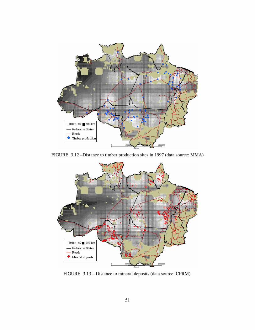
51
FIGURE 3.12 –Distance to timber production sites in 1997 (data source: MMA)
FIGURE 3.13 – Distance to mineral deposits (data source: CPRM).

52

53
FIGURE 3.14 - Population density in 1996 (data source: IBGE Population Counting 1996).

54

55
FIGURE 3.15 – Technological indicator: average number of tractors per property in 1996 (data source: IBGE Agricultural Census 1996).
FIGURE 3.16 - Technological indicator: percentage of farms that received technical assistance in 1996 (data source: IBGE Agricultural Census 1996).

56
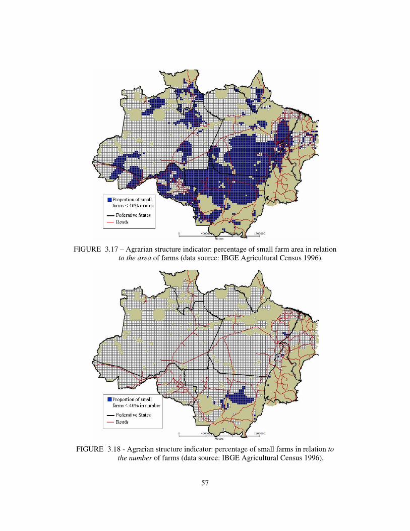
57
FIGURE 3.17 – Agrarian structure indicator: percentage of small farm area in relation to the area of farms (data source: IBGE Agricultural Census 1996).
FIGURE 3.18 - Agrarian structure indicator: percentage of small farms in relation to
the number of farms (data source: IBGE Agricultural Census 1996).

58

59
FIGURE 3.19 – Number of settled families from 1970 to 1999 (data source: INCRA).
FIGURE 3.20 – Percentage of protected areas in 1997: Indigenous Lands and Federal and State Conservation Units (data sources: MMA and FUNAI).

60
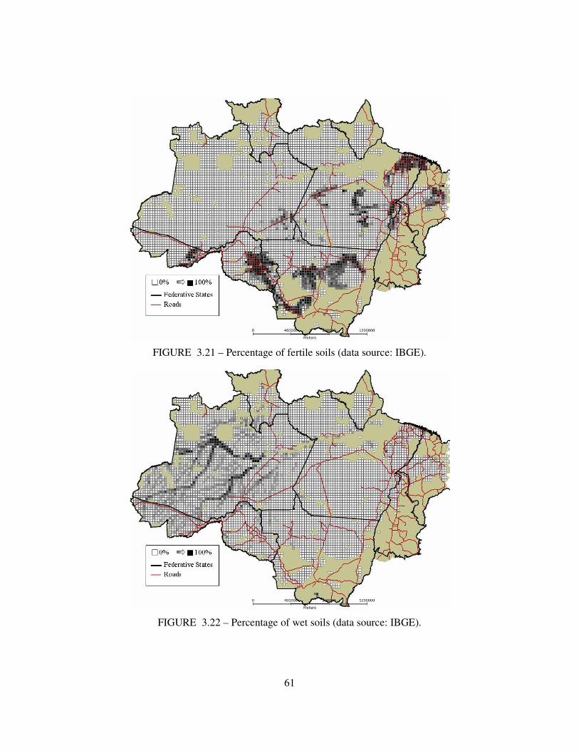
61
FIGURE 3.21 – Percentage of fertile soils (data source: IBGE).
FIGURE 3.22 – Percentage of wet soils (data source: IBGE).

62

63
FIGURE 3.23 - Average humidity in the three driest consecutive months of the year (data source: INMET).
FIGURE 3.24 - Average precipitation in the three less rainy consecutive months of the year (data source: INMET).

64

65
CHAPTER 4
SPATIAL MODELING OF LAND-USE DETERMINANTS IN THE BRAZILIAN
AMAZONIA
4.1 Introduction
This chapter presents the development of a spatial explicit model of the determinants
associated to land use change in Amazonia, using the 25 x25 km2 cells of the database
presented in Chapter 3.
The model explores the relative importance of the determining factors related to
deforestation, pasture, temporary and permanent agriculture patterns, and the intra-
regional differences between these factors. Four spatial partitions are compared: the
whole Brazilian Amazonia and three macro-regions defined by Becker (2005), namely
the Densely Populated Arch, the Central Amazonia and the Oriental Amazonia (Figure
1.1). Results are consistent with the hypothesis of heterogeneity adopted in this thesis.
This chapter is organized as follows. Section 4.2 presents the methods used in the
assessment of determinant factors for land use patterns in Amazonia. Section 4.3
presents the results and discusses them.
4.2 Methods
4.2.1 Exploratory analysis and selection of variables
In the statistical models of this chapter, dependent variables are those associated to land
use (deforestation, pasture, temporary and permanent agriculture). The potential
explanatory variables were grouped into seven types: accessibility to markets,
economical attractiveness, demographical, technological, agrarian structure, public
policies, and environmental, as described in Chapter 3.

66
An initial exploratory statistical analysis showed that some of the relationships between
potential explanatory variables and the land use variables were not linear. We applied a
logarithmic transformation to the land use variables and to some explanatory variables.
The log transformation improved the regression results significantly. This improvement
suggests that the explanatory variables are related to the initial choice of areas to be
occupied. After the initial choice, land use change behaves as a spatial diffusion process
because deforestation tends to occur close to previously deforested areas (Alves, 2002).
There was a high degree of correlation among potential explanatory factors. This led to
the selection of a subset of the initial 50 potential variables. When choosing between
highly correlated variables, those related to accessibility and public policies had
preference. For the same category, alternative possibilities were tested. For instance, out
of the many environmental variables, we chose the average humidity in the drier
months. The final choice of explanatory variables for regression analysis does not
include demographical or technological factors, which are captured indirectly by other
variables. As a result, the statistical analysis used only a representative subset of all
variables, as shown in Table 4.1. This subset was selected to cover the broadest possible
range of categories, while minimizing correlation problems.

67
TABLE 4.1 – Subset of potential explanatory variables selected for the spatial statistical analysis.
Even in the subset of variables presented above, there was still a high degree of
correlation, which varied across the spatial partitions. We decided to build different
spatial regression models, where each model had potentially explanatory variables with
less than 50% correlation between them. To build the regression models, we selected as
primary variables those with potentially greater explanatory power in relation to
deforestation: distance to urban centres, distance to roads, climatic conditions and
connection to markets. Then we tested these three variables for correlation to select the
Category Variable Description Unit Source Accessibility to markets
conn_mkt Indicator of strength of connection to national markets (SP and NE) through roads network
- IBGE
conn_ports Indicator of strength of connection to ports through roads network
- IBGE
log_dist_rivers Euclidean distance to large rivers (log)
km IBGE
log_dist_roads Euclidean distance to roads (log)
km IBGE
log_dist_urban Euclidean distance to urban centers (log)
km IBGE
Economic Attractiveness
log_dist_wood Euclidean distance to wood extraction poles (log)
km IBAMA
log_dist_mineral Euclidean distance to mineral deposits (log)
km CPRM
Public policies prot_area Percentage of protected areas % of cell area
IBAMA FUNAI
log_settl Number of settled families from 1970 to 1999 (log)
Number of families (log)
INCRA
Agrarian Structure
agr_small Percentage of area of small properties
% of cell area
IBGE
Environmental soil_fert Percentage of high and medium to high fertility soils in
% of cell area
IBGE
soil_wet Percentage of wetland soils (“várzea” soils)
% of cell area
IBGE
clim_humid Average humidity in the three drier months of the year
% INMET

68
leading variables for each model. Distance to urban centres and distance to roads were
correlated in all spatial partitions, except in the Occidental one. Distance to roads and
connection to national markets could not be placed in the same subgroup for the whole
Amazon. Climatic conditions and connection to national markets were also highly
correlated, except in the Central region. This cross-correlation analysis between the
potentially explanatory variables led to the models summarized in Table 4.2. An
automatic linear forward stepwise regression was applied to refine the models and
discard non-significant variables. Some variables were found to be significant in some
of the models and non-significant in others, as shown in Table 4.2. The resulting models
are:
1. Amazonia: for the whole region, three models were considered: one including
distance to urban centres and connection to markets (urban+connection), one
including distance to urban centres and climatic conditions (urban+climate), and
a third one including distance to roads and climatic conditions (roads+climate).
2. Densely Populated Arch: for this region, two models are considered. The first is
lead by distance to urban centres and connection to markets (urban+connection)
and the second includes distance to roads and connection to markets
(roads+connection).
3. Central Amazonia: for this region, two models are considered. The first is lead
by distance to urban centres and connection to markets (urban+connection) and
the second includes distance to roads and connection to markets
(roads+connection).
4. Central Amazonia: for this region, a single model that includes distance to urban
centres, distance to roads, and connection to markets (urban+roads+connection)
was considered.

69
TABLE 4.2 - Groups of non-correlated explanatory variables for the spatial statistical analysis.
4.2.2 Spatial regression modeling
Spatial regression models were used to establish the relative importance of the
determining factors for different land-uses. One of the basic hypotheses in linear
regression models is that observations are not correlated, and consequently the residuals
of the models are not correlated too. In land use data, this hypothesis is frequently not
true. Land use data has the tendency to be spatially autocorrelated. The land use changes
in one area tend to propagate to neighbouring regions. Spatial dependence could be seen
as a methodological disadvantage, as it interferes on linear regression results, but on the
other hand is exactly what gives us information on spatial pattern and structure and
Amazonia Arch Central Occidental
urba
n+co
nnec
tion
urba
n+cl
imat
e
road
s+cl
imat
e
urba
n+cl
imat
e
road
s+co
nnec
tion
urba
n+cl
imat
e+co
nnec
tion
road
s+cl
imat
e+co
nnec
tion
urba
n+ro
ads
log_dist_urban x x x x x
log_dist_roads x x x x
conn_mkt x x x x n/s
clima_humid x x x x x n/s
conn_ports x x x n/s n/s x x n/s
log_dist_rivers x x x n/s n/s x x x
log_dist_wood x x
log_dist_mineral x x x x x
prot_area x x x x x x x x
agr_small x x x x x x n/s n/s
log_settl x x x x x x x x
soil_fert x x x x x x x n/s
soil_wet x n/s x n/s n/s x x n/s

70
process (Overmars et al., 2003). This work applies a spatial lag regression model
(Anselin, 2001) to assess the relative importance of potential explanatory factors. In this
method, the spatial structure is supposed to be captured in one parameter.
The linear regression model formulation can be described as:
),N(~,ε 20 σε+= XβY , or (4.1)
+
=
−−
−
−
nknkn
k
k
n
..
..
..
..
x..x
........
........
x..x
x..x
y
..
..
y
y
ε
ε
ε
β
β
β
2
1
1
1
0
11
1221
1111
2
1
1
1
1
(4.2)
where Y is an (n x 1) vector of observations on a dependent variable taken at each of n
locations, X is an (n x k) matrix of exogenous variables, ββββ is an (k x 1) vector of
parameters, and εεεε is (n x 1) an vector of disturbances. The spatial lag model includes a
spatial dependence term, through a new term that incorporates the spatial
autocorrelation as part of the explanatory component of the model:
ερ ++= XβWYY (4.3)
where W is the spatial weights matrix, and the product WY expresses the spatial
dependence on Y, where ρ is the spatial autoregressive coefficient. The spatial
autoregressive lag model aims at exploring the global patterns of spatial autocorrelation
in the data set. This spatial model considers that the spatial process whose observations
are being analyzed is stationary. This implies that the spatial autocorrelation patterns
can be captured in a single regression term. This method was employed by Overmars et
al. (2003) in a study in Equador. In the Brazilian Amazon, Perz and Skole (2003) used a
spatial lag model, focusing on social factors related to secondary vegetation.
In this work, we compare the results of the spatial lag models with those of a non-spatial
linear regression model for the whole Amazonia. This helps to understand how

71
explanatory factors contribute to spatial dependence in this case. These results will be
presented in the next section. In order to compare the models, we will present the R2
value (coefficient of multiple determination) and the Akaike information criteria (AIC).
As stated by Anselin (2001), the R2 value is not a reliable indicator of goodness of fit
when the data is spatially autocorrelated. The Akaike information criteria (Akaike,
1974) is a more suitable performance measure than the R2 value for spatially correlated
data. The model with the highest AIC absolute value is the best. To compare the
determining factors relative importance in each model, the standardized regression
coefficients (beta) and associated significance level (p-level) for each variable will be
presented.
4.3 Results and discussion
This section summarizes the main findings, organized as follows. Section 4.1 presents
the deforestation determining factors for whole Amazonia. It compares the results
obtained by linear regression to those of spatial regression. The comparison shows how
determinants change their importance when spatial autocorrelation is considered, and
what this indicates in terms of spatial dependence and land-use structure. Section 4.2
presents a comparison of deforestation factors across the four spatial partitions
(Amazonia, Densely Populated Arch, Central and Occidental macro-zones), using
spatial regression models. Section 4.3 presents a comparison of the main land-use
(pasture, temporary and permanent agriculture) determinants, also using spatial
regression models. The results of pasture and agriculture determinants are presented
only for the Arch macro-zone, where occupation is more consolidated.
4.3.1 Deforestation factors in the whole Amazonia
This section presents and discusses the regression models for whole Amazonia. A pre-
processing step maintained in the models only variables less than 50% correlated to
each other, and eliminated those non-significant according to an automatic forward
stepwise procedure (see Table 4.2). The three models have the following explanatory
variables:

72
• urban+connection: distance to urban centres (log), connection to markets,
connection to ports, distance to rivers (log), protected areas, percentage of small
farmers, number of families in settlements (log), soil fertility, and soil wetness.
• urban+climate: distance to urban centres (log), humidity, connection to ports,
distance to rivers (log), distance to mineral deposits (log), protected areas,
percentage of small farmers, number of families in settlements (log), soil
fertility, and soil wetness.
• roads+climate: distance to roads (log), humidity, connection to ports, distance to
rivers (log), protected areas, percentage of small farmers, number of families in
settlements (log), soil fertility, and soil wetness.
Table 4.3 presents the statistical analysis results for the three models and compares the
non-spatial linear regression model with the spatial lag model, where the dependent
variable is the log percentage of deforestation for each 25 x 25 km2 cell. The spatial lag
model includes one additional variable (w_log_def) that measures the extent of
spatial autocorrelation in the deforestation process. In Table 4.3, we present the R2 value
(coefficient of multiple determination) and the Akaike information criteria (AIC) for all
models. In both indicators, the spatial regression models showed a better performance
than the non-spatial linear model. The spatial coefficient of the spatial lag models is
significant and higher than 0.70 in all models. This is a quantitative evidence that
corroborates of earlier assessments that deforestation is a diffusive process in the
Amazon, and tends to occur close of previously opened areas (Alves, 2002). The other
variables found to be important (with higher betas) are distance to urban centres (log),
distance to roads (log), connection to markets, humidity, and protected areas.

73
TABLE 4.3 - Linear and spatial lag regression models of (log) deforestation determining factors in the whole Amazon.
We also compared the strength of the most important factors considering the linear
regression model and the spatial lag model, as shown in Table 4.4. It groups the distance
to urban centres and distance to roads variables that are highly correlated, and then
connection to markets and climate variables, also highly correlated. As expected, using
the spatial lag regression model, all betas get lower, but not in a uniform way. When
considering the intrinsic spatial dependence of deforestation, the ‘connection to
markets’ variable (and the climate one) decreases proportionally more than the others,
although it is still one of the main factors. Therefore, these variables carry a large part
Subgroup urban+connection Subgroup urban+climate Subgroup roads+clima
Linear Regression R-squared: 0.66 R-squared: 0.65 R-squared: 0.58 AIC: -39144.50 AIC: -38944.9 AIC: -37928.6 Beta p-level Beta p-level Beta p-level log_dist_urban -0.45 0.00 log_dist_urban -0.48 0.00 log_dist_road -0.39 0.00 conn_mkt 0.26 0.00 clim_humid -0.18 0.00 clim_humid -0.24 0.00 prot_area -0.14 0.00 log_settl 0.12 0.00 prot_area -0.19 0.00 log_settl 0.10 0.00 prot_area -0.15 0.00 soil_fert 0.16 0.00 soil_fert 0.09 0.00 soil_fert 0.12 0.00 log_settl 0.13 0.00 conn_ports 0.07 0.00 agr_small -0.10 0.00 soil_wet 0.10 0.00 agr_small -0.09 0.00 conn_ports 0.07 0.00 log_dist_rivers -0.07 0.00 log_dist_rivers -0.04 0.00 log_dist_mineral -0.05 0.00 conn_ports 0.05 0.00 soil_wet -0.02 0.02 log_dist_rivers -0.03 0.00 agr_small -0.06 0.00
Spatial Lag R-squared: 0.81 R-squared: 0.81 R-squared: 0.81 AIC: -41876.2 AIC: -41871 AIC: -41781.5 Beta p-level Beta p-level Beta p-level w_log_def 0.73 0.00 w_log_def 0.74 0.00 w_log_def 0.78 0.00 log_dist_urban -0.15 0.00 log_dist_urban -0.16 0.00 log_dist_road -0.13 0.00 conn_mkt 0.05 0.00 clim_humid -0.04 0.00 clim_humid -0.05 0.00 prot_area -0.07 0.00 log_settl 0.03 0.00 prot_area -0.07 0.00 log_settl 0.03 0.00 prot_area -0.07 0.00 soil_fert 0.04 0.00 soil_fert 0.03 0.00 soil_fert 0.03 0.00 log_settl 0.02 0.01 conn_ports 0.02 0.00 agr_small -0.03 0.00 soil_wet 0.05 0.00 agr_small -0.03 0.00 conn_ports 0.02 0.00 log_dist_rivers -0.03 0.00 log_dist_rivers -0.03 0.00 log_dist_mineral -0.02 0.01 conn_ports 0.01 0.14 soil_wet 0.01 0.05 log_dist_rivers -0.02 0.00 agr_small -0.01 0.18

74
of the spatial dependence. This corroborates with earlier assessments (Alves, 2002) that
showed that deforestation tends to occur along roads that provide an easier connection
to the more developed areas in Brazil. These areas also present the driest climate in
Amazon, with more favourable conditions to agriculture (and also to infra-structure
construction and maintenance) than the more humid areas in the western Amazonia, in
accordance with previous results (Schneider, 2000). Our statistical results indicate that
these factors (the diffusive nature of deforestation, distance to roads and to urban
centres, climate and connection to markets), and the interaction among them,
contributed significantly for the pattern of deforestation in 1996/1997. The existence of
protected areas also plays an important role in avoiding deforestation in high pressure
areas, as will be further discussed in the next section.
TABLE 4.4 - Main deforestation determining factors comparison (whole Amazonia).
Previous studies of causes of land-use change in Amazonia tended to emphasize
distance to roads as the main determinant (Kirby et al., 2006; Laurance et al., 2002).
The results from this paper indicate that distance to urban centres is as important as
distance to roads as a determinant factor for land-use change. Distance to urban centres
is a population indicator and also a proxy of local markets. In 1996, 61% of the
Variable Subgroup Beta % of Linear Spatial lag decrease
w_log_def urban+connection - 0.73 - w_log_def urban+climate - 0.74 - w_log_def roads+climate - 0.78 - log_dist_urban urban+connection -0.45 -0.15 67% log_dist_urban urban+climate -0.48 -0.16 67% log_dist_roads roads+climate -0.39 -0.13 67% conn_mkt urban+connection 0.26 0.05 81% clim_humid urban+climate -0.18 -0.04 78% clim_humid roads+climate -0.24 -0.05 79% prot_area urban+connection -0.14 -0.07 50% prot_area urban+climate -0.15 -0.07 53% prot_area roads+climate -0.19 -0.07 63%

75
approximately 20 million people lived in Amazonian urban areas; in 2000, 69% of the
total population (Becker, 2004). Urban population growth rates increase faster in
Amazonia than in other parts of Brazil, not only in the larger cities but also in those with
less than 100.000 people (Becker, 2001). Faminow (1997) showed that the local
demand for cattle products such as beef and milk is an overlooked cause of cattle
production increase, and consequently, deforestation. Our results reinforce the need to
further understand the relationship between land use change and this process of urban
population growth in Amazônia.
In summary, our results indicate that strong spatially concentrated pattern of
deforestation in Amazonia is related to the diffusive nature of the land use change
process. The concentration of this pattern in the Southern and Eastern parts of the
Amazonia is related to proximity to urban centres and roads, reinforced by the higher
connectivity to the more developed parts of Brazil, and more favourable climatic
conditions in comparison to the rest of the region. Therefore, more favourable
production conditions in terms of climate, connection to national markets, and
proximity to local markets seem to be the key factors in explaining the deforestation
process.
4.3.2 Comparison of deforestation determining factors across space partitions
This section presents and discusses the regression models for three spatial partitions:
Densely Populated Arch, Central Amazonia and Occidental Amazonia. For each space
partition, two alternative models were considered, one including the distance to urban
centres variable, and one with the distance to roads variable (except in the Occidental
partition where they were allowed to be in the same model). A pre-processing step
maintained in the models only variables less than 50% correlated to each other, and
eliminated those non-significant according to an automatic forward stepwise procedure
(see Table 4.2). The models have the following explanatory variables:
• Arch: urban+climate: distance to urban centres (log), climate, distance to timber
production (log) distance to mineral deposits (log), protected areas, percentage
of small farmers, number of families in settlements (log), and soil fertility;

76
• Arch: roads+connection: distance to roads (log), connection to markets, distance
to timber production (log), distance to mineral deposits (log), protected areas,
percentage of small farmers, number of families in settlements (log), and soil
fertility.
• Central: urban+climate+connection: distance to urban centres (log), connection
to markets, humidity, connection to ports, distance to rivers (log), distance to
timber production (log), distance to mineral deposits (log), protected areas,
percentage of small farmers, number of families in settlements (log), soil
fertility, and soil wetness;
• Central: roads+climate+connection: distance to roads (log), connection to
markets, humidity, connection to ports, distance to rivers (log), distance to
timber production (log), distance to mineral deposits (log), protected areas,
number of families in settlements (log), soil fertility, and soil wetness.
• Occidental: urban+roads: distance to urban centres (log), distance to roads
(log), distance to rivers (log), protected areas, and number of families in
settlements (log).
Table 4.5 presents the statistical analysis results for these models, including the R2 and
the Akaike information criteria (AIC). Both criteria indicate that the Arch models are
the best fit. The spatial autoregressive coefficient (w_log_def) is significant and
higher than 0.67 in all models of the Arch and Central regions. In the Occidental region,
it is also significant, but presents a lower value (0.54), indicating a less marked spatial
pattern. The Occidental region is still quite undisturbed, except by the areas close to the
main rivers, and around Manaus. As stated by Becker (2001) the Amazonia presents
regions with different speeds of modification. The lower spatial dependence is an
indicator that occupied areas in the Occidental region do not spread to the neighbouring
cells at the same pace as the ones in the main axes of development in the Arch and
Central region. The other variables found to be important (with higher betas) - or that
present some relevant variation among the spatial partitions - are: distance to urban

77
centres (log), distance to roads (log), protected areas, connection to markets, connection
to ports, distance to large rivers, soil fertility, number of settled families, and agrarian
structure. Figure 4 illustrates graphically the most important differences found among
these eight factors.
TABLE 4.5 - Spatial lag regression models of deforestation determining factors across space partitions.
ARCH CENTRAL OCCIDENTAL Distance to roads models
R-squared: 0.80 R-squared: 0.71 R-squared: 0.50
AIC : -14783.70 AIC : -12413.10 AIC : -12023.00
Beta p-level Beta p-level Beta p-level
w_log_def 0.71 0.00 w_log_def 0.72 0.00 w_log_def 0.54 0.00
conn_mkts 0.07 0.00 log_dist_roads -0.16 0.00 log_dist_urban -0.24 0.00
prot_areas -0.19 0.00 conn_ports 0.07 0.00 log_dist_roads -0.15 0.00
log_dist_roads -0.12 0.00 log_dist_rivers -0.07 0.00 log_dist_rivers -0.08 0.00
log_dist_wood -0.04 0.00 log_settl 0.04 0.01 prot_area -0.02 0.17
soil_fert 0.04 0.00 prot_area -0.06 0.00 log_settl 0.00 0.81
log_settl 0.02 0.05 soil_wet 0.07 0.00 agr_small -0.03 0.01 log_dist_mineral -0.05 0.00 log_dist_mineral -0.01 0.20 conn_mkt 0.03 0.06 clim_humid -0.07 0.00
soil_fert 0.03 0.06
Distance to urban models
R-squared: 0.80 R-squared: 0.71
AIC : -13942.20 AIC : -12405.10
Beta p-level Beta p-level
w_log_def 0.70 0.00 w_log_def 0.67 0.00
log_dist_urban -0.16 0.00 log_dist_urban -0.17 0.00
prot_areas -0.19 0.00 conn_ports 0.09 0.00
clim_humid -0.05 0.00 conn_mkt 0.07 0.00
log_settl 0.03 0.00 prot_area -0.07 0.00
soil_fert 0.03 0.00 log_dist_mineral -0.05 0.00
log_dist_mineral -0.03 0.02 log_settl 0.04 0.00
agr_small -0.03 0.01 soil_wet 0.05 0.00
log_dist_wood -0.02 0.05 clim_humid -0.06 0.00
log_dist_rivers -0.05 0.00
soil_fert 0.03 0.04
agr_small 0.01 0.68

78
FIGURE 4.1 - Graphical comparison of main deforestation factors across macro-regions. Values shown are the average of significant beta coefficients. Empty values are non-significant coefficients in any of the models for that partition.
The first main difference is the relative higher values of the protected areas variable (%
of all types of protected areas in each cell, including Indigenous Lands and Federal and
State Conservation Units). In the Arch, it is the second most important factor (after the
spatial autocorrelation coefficient), preceding distance to roads and distance to urban
centers. Indigenous lands and conservation units correspond, respectively, to 22% and
6% of the Amazon region (Becker, 2001), spread over the region (see Figure 3.20). Our
results indicate quantitatively that protected areas can be important instruments in
avoiding deforestation in high pressure areas such as the Arch. This is in accordance
with earlier results that showed that protected areas are in general effective in refraining
deforestation even if some level of deforestation is found inside of them Ferreira et al.
(2005). Their efficacy depends on the clear demarcation of its limits, on the socio-
economic context in which they are created, and on appropriate monitoring and
controlling measures, as discussed by Ribeiro et al. (2005) and Escada et al. (2005a).
Distance to roads and distance to urban centers are not the most important determinants
in all macro-regions. Also, they do not explain intra-regional differences, as they are
both similarly important in all macro-zones, except in the Occidental macro-zone,

79
where distance to urban centers is considerably more important. In the Occidental
macro-zone, distance to large rivers also plays an important role. This result is coherent
with the small disturbance of the area, concentrated mostly in Manaus and close to the
rivers.
On the other hand, connection measures (connection to markets and connection to ports)
play different roles across the partitions. Connection to markets is important in
explaining Arch deforestation patterns, but not in the other macro-regions. In the
Central macro-region it looses significance in one of the models, when distance to roads
is also used. Connection to ports is important only in the Central region, whose
historical occupation process is related to the rivers. Climate (intensity of dry season) is
also important in explaining deforestation in the Arch and Central partitions. In the
Central spatial partition, the climate variable did not present correlation to the
connection to markets variable, and both could be placed in the same regression model.
In the Arch, climate and connection to markets are correlated, and were analyzed in
different models, both presenting significant coefficient values. This indicates that both
factors created favourable conditions to occupation in the Eastern part of the Amazon.
The differences between the models for the Arch and the Central regions are important.
They point out to an occupation process in the Arch that uses roads as its main
connections. In the Arch, the existence of protected areas is the main factor that is
statistically significant as an impediment to deforestation. A second deterrent is
unfavourable climatic conditions, in areas where the dry season is more intense. Since
the area on the south of the Arch still has a considerable extension of primary forest
areas outside protected areas, close to the mechanized agriculture belt in the south of
Mato Grosso, and also benefits from drier climate, the creation of protected areas in that
region would be an important factor for deterrence of the deforestation process.
In the Central region, due to its historical occupation process, connection to national
markets is not significant in one of the models. There is a stronger influence of rivers
connections (variables distance to rivers and connection to ports). The Central region is
currently the most vulnerable region, where new frontiers are located (Becker, 2004).

80
As the agricultural production systems of the new occupied areas in the Central region
became stronger, these statistical relationships will be modified to reflect the new
reality, but not necessarily replicating the Arch relationships. For instance, connection
to ports may continue to be important in the Central region due to the presence of
exportation ports in the Amazon River, but road connection to the rest of the country
may also gain importance, linking productive areas to their markets. In relation to
protected areas, the statistical relationship was not as strong as in the Arch in the period
of analysis. However, the creation of protected areas in the Central region, in
appropriate socio-economic contexts (Escada et al., 2005a), would also be an important
instrument for conservation of areas that may become threatened by the new frontiers.
In the next paragraphs we discuss results related to other significant variables: soils
fertility, number of settled families and agrarian structure indicators. The soils fertility
indicator (percentage of fertile soils in each cell) has a positive relationship to
deforestation in the Arch and in the whole Amazonia models. Comparing the
deforestation patterns and the patterns of medium and high fertility soils in the 25 x 25
km2 cell space shown 3.21, one can notice the existence of better quality soils in
Rondônia and the Transamazônica, where most colonization programs were placed.
Better soils are also found in Mato Grosso. Federal Government possibly took into
consideration existing soil surveys when planning the development projects and
colonization settlements of the 70’s and 80’s (the RADAM project in the 70’s mapped
vegetation, soils, geology and geomorphology).
As expected, the number of settled families by official colonization programs
(accumulated from 1970 to 1999) has a positive and significant relationship in the Arch
and Central regions (and also in the whole Amazonia, as Table 4.3 shows). On the other
hand, the agrarian structure indicator (percentage in area of farms smaller than 200 ha)
is also significant in the Arch, but presents a negative signal, indicating that
deforestation is more associated with areas with a greater proportion of medium and
large farms, than areas occupied by small farms. This relationship is also significant in
the whole Amazonia.

81
Many authors have presented diverse estimates of the share of small and large farmers
in relation to deforestation (for instance, Fearnside (1993); Walker et al. (2000). As
stated by Walker et al. (2000) and Margulis (2004), the relative importance of small,
medium and large farms on deforestation varies from one region to the other, as the
dynamics of deforestation are very distinct at different localities. However most of
previous works show that when considering the overall deforestation extent in the
Amazon a more significant impact is caused by large farms (Margulis, 2004). Our
results provide further evidence that areas occupied by large and medium farms have a
higher impact on deforestation than areas occupied by small farms, when the whole
Arch macro-region is analyzed. This can be explained by the relative contribution of
Pará, Tocantins and Mato Grosso states. As Figure 4.2 illustrates, small farm areas are
concentrated in Rondônia, northeast of Pará and Maranhão. In most of the Arch area,
the agrarian structure is predominantly of medium and large farms. For instance, in
Mato Grosso the mean value for the agrarian structure indicator is 0.07 (0.07 standard
deviation), meaning that in average only 7% of the farm lands are occupied by
properties with less than 200 ha.
FIGURE 4.2 - Agrarian structure and deforestation patterns in the Arch.

82
4.3.3 Comparison of land-use determining factors in the Arch partition
This section presents and discusses the results of the spatial lag models for the Arch
partition, in which the dependent variables are the log percentage of pasture, temporary
agriculture and permanent agriculture in each 25 x 25 km2 cell. For each of these three
types of land use, we consider two alternative models, one including the distance to
urban centres variable, and one with the distance to roads:
• urban+climate: distance to urban centres (log), climate, distance to timber
production (log) distance to mineral deposits (log), protected areas, percentage
of small farmers, number of families in settlements (log), and soil fertility;
• roads+connection: distance to roads (log), connection to markets, distance to
timber production (log), distance to mineral deposits (log), protected areas,
percentage of small farmers, number of families in settlements (log), and soil
fertility.
Table 4.6 presents the statistical analysis results for the six models. The R2 and the
Akaike information criteria (AIC) are presented as measures of goodness of fit to
compare the models. All indices are similar, but temporary agriculture models perform
slightly better according to the log likelihood. The spatial auto-regressive coefficient of
the spatial lag models is significant and higher than 0.70 in all models, presenting the
higher values in the permanent agriculture models (above 0.80), indicating a stronger
clustering of such use (see Figure 2). The other relevant factors that will be analyzed in
this section are: distance to urban centres (log), distance to roads (log), protected areas,
connection to markets, and agrarian structure. Figure 4.3 illustrates graphically the most
important differences found among these eight factors.
As with deforestation in the Arch macro-region, protected areas, distance to roads and
distance to urban centres are the most important variables in explaining the distribution
of land-use patterns. Connection to markets is significant to temporary agriculture and
pasture, but not to permanent agriculture. The main difference is the signal in relation to
agrarian structure variable (percentage in area of farms smaller than 200 ha). The beta

83
value for the agrarian structure has a positive value in both temporary agriculture and
permanent agriculture models. In the pasture model, the beta is negative.
TABLE 4.6 - Spatial lag regression models of pasture, temporary and permanent agriculture in the Arch.
ARCH CENTRAL OCCIDENTAL Distance to roads models
R-squared: 0.80 R-squared: 0.71 R-squared: 0.50
AIC : -14783.70 AIC : -12413.10 AIC : -12023.00
Beta p-level Beta p-level Beta p-level
w_log_def 0.71 0.00 w_log_def 0.72 0.00 w_log_def 0.54 0.00
conn_mkts 0.07 0.00 log_dist_roads -0.16 0.00 log_dist_urban -0.24 0.00
prot_areas -0.19 0.00 conn_ports 0.07 0.00 log_dist_roads -0.15 0.00
log_dist_roads -0.12 0.00 log_dist_rivers -0.07 0.00 log_dist_rivers -0.08 0.00
log_dist_wood -0.04 0.00 log_settl 0.04 0.01 prot_area -0.02 0.17
soil_fert 0.04 0.00 prot_area -0.06 0.00 log_settl 0.00 0.81
log_settl 0.02 0.05 soil_wet 0.07 0.00 agr_small -0.03 0.01 log_dist_mineral -0.05 0.00 log_dist_mineral -0.01 0.20 conn_mkt 0.03 0.06 clim_humid -0.07 0.00
soil_fert 0.03 0.06
Distance to urban models
R-squared: 0.80 R-squared: 0.71
AIC : -13942.20 AIC : -12405.10
Beta p-level Beta p-level
w_log_def 0.70 0.00 w_log_def 0.67 0.00
log_dist_urban -0.16 0.00 log_dist_urban -0.17 0.00
prot_areas -0.19 0.00 conn_ports 0.09 0.00
clim_humid -0.05 0.00 conn_mkt 0.07 0.00
log_settl 0.03 0.00 prot_area -0.07 0.00
soil_fert 0.03 0.00 log_dist_mineral -0.05 0.00
log_dist_mineral -0.03 0.02 log_settl 0.04 0.00
agr_small -0.03 0.01 soil_wet 0.05 0.00
log_dist_wood -0.02 0.05 clim_humid -0.06 0.00
log_dist_rivers -0.05 0.00
soil_fert 0.03 0.04
agr_small 0.01 0.68

84
FIGURE 4.3 - Graphical comparison of main land-use factors in the Arch macro-region.
Values shown are the average of significant beta coefficients. Empty values are non-
significant coefficients in any of the models for that partition.
Pasture is spread over the region (see Figure 3.3), and its determining factors are very
similar to deforestation ones, discussed in previous section. Our results indicate that
medium and large farms have a larger proportion of pasture areas when considering the
whole Arch extent. The relative share of small, medium and large farms in terms of
pasture area varies according different localities. Rondônia, for instance, have a
significant pasture area (see Table 3.1) and an agrarian structure related to small
farmers. The negative signal our model captures is related to the proportionally larger
area of Mato Grosso and Pará States, in which the agrarian structure is predominantly
of large farms.
On the other hand, temporary and permanent agriculture present differentiated and
concentrated patterns, as discussed in Section 3.2. Our results indicate a tendency for
temporary and permanent agriculture to occupy areas associated to small farms, when
considering the whole Arch, in our period of analysis. Permanent crops are present in
North-eastern Pará, Rondônia and along the Amazon River. These three areas have a
land structure related mostly to small properties, what explains the positive signal in the
permanent agriculture model. In the temporary agriculture model, the positive signal

85
can be explained by the fact that the temporary agriculture practiced in Pará and
Maranhão by small farmers occupy a larger area than the mechanized agriculture found
in the south of Mato Grosso (see Table 3.1). Although this statistical relationship may
change with the expansion of mechanized agriculture into forest areas (Becker, 2005),
that requires large tracts of plain land, and is practiced by a capitalized type of actor, our
results indicate the existence of a land use system based on temporary agriculture
practiced by small farms, especially in old occupation areas such as Maranhão and
Northeast Pará.
This land use pattern analysis we conducted provide further evidence of the
heterogeneity of the region, both in terms of agrarian structure and land use trajectories
adopted in different localities. For instance, both Rondônia and the north-eastern part of
Pará State have a dominance of small farms. However, in Rondônia temporary crops are
not as significant as in north-eastern Pará. On the other hand, there is a significant
pattern of permanent crops in Rondônia. Soybean expansion may change the statistical
relationship with the agrarian structure as we obtained for temporary crops, but not the
fact that these other land use systems exist, and that effective policy action may take this
heterogeneity into consideration.

86

87
CHAPTER 5
EXPLORING SCENARIOS OF LAND-USE CHANGE IN THE BRAZILIAN
AMAZONIA
5.1 Introduction
In this chapter a dynamic spatially explicit model (the CLUE model (Kok et al., 2001;
Veldkamp and Fresco, 1996; Verburg et al., 1999a)) is applied to explore possible
scenarios of land use change in the Brazilian Amazonia. The concept of “scenario
exploration” is introduced. Each exploration emphasizes a different aspect of the
Amazonia occupation process. Out of many possibilities, this work presents the results
of five explorations which analyze the effects on future deforestation patterns of
alternative accessibility factors, policies and market constraints, as follows.
The two first explorations analyze the use of alternative regression models in the CLUE
framework to identify factors that best capture the new Amazon frontiers and future
possible axes of development. This comparison aims at understanding the importance of
different accessibility determining factors in process of land use change. In the first
exploration, the focus is on connectivity factors. In the second, accessibility to local
markets (distance to urban centres). Then, the impacts of alternative public policies are
analyzed in two other explorations. Two types of policies are considered: (a) policies
that influence intra-regional conditions for agricultural use, such as road paving and the
creation of protected areas; and (b) law enforcement policies, such as deforestation
limits inside private properties. Last exploration analyzes scenarios of increasing and
decreasing demand for land in Amazonia, corresponding to higher or lower pressure for
forest conversion determined by the national and international agribusiness.
From each of the five explorations very different patterns may emerge. Each exploration
comprises two or three alternative results (hot-spots of change from 1997 to 2020) to be

88
compared. Together, the results of the five explorations are complementary, and
contributing to the understanding of different aspects of the occupation process.
This chapter is organised as follows. Section 5.2 presents the methodology. Section 5.3
presents the results and discussion of the different scenario explorations.
5.2 Methods
5.2.1 The CLUE framework and its adaptation to Amazonia
This paper uses the CLUE framework adapted to the Amazonia characteristics. The
CLUE framework consists of two main components, as illustrated in Figure 5.1 6: (1)
the Demand module, that projects the amount of change for each land-use class; (2) the
Allocation module, the spatial component that acts in two scales (a coarse and a fine
resolution grid) to localize such changes. The demand module is application specific
(see, for instance, previous CLUE applications in Ecuador (De Koning et al., 1999)
China (Verburg and Veldkamp, 2001; Verburg et al., 1999b), and Central America (Kok
and Veldkamp, 2001.)). Demand calculation is based either on trend analysis of past
change rates, scenario constructions, or more elaborate economical models. The amount
of change for each land use is passed on to the allocation module. The allocation
module uses one cellular space consisting of fixed size cells for each spatial scale.
Allocation of changes depends on the suitability of each cell, defined by empirical
relationships between land use patterns and determining factors.

89
FIGURE 5.1 - Structure of the main components of the CLUE modeling framework (source: adapted from Verburg et al. (1999b)).
The CLUE multi-scale allocation module works as follows. Relations between land uses
and explanatory factors are quantified by multiple regressions based on land use
patterns in a given date. Different regression models are adopted at the coarse and fine
resolution. Such regression models are used to establish the suitability of each cell in
relation to a certain land use. The model first allocates changes at coarse resolution cells
trying to reach the total amount of change determined by the demand module for each
land-use in each year. Then the same process is repeated at fine scale. The difference,
besides the use of different regression models, is that the amount of change in each cell
at fine scale is also influenced by the change projected at the corresponding cell at
coarse scale. Details about the allocation mechanism can be found in Verburg et al.
(1999a).
Adapting the CLUE framework to Amazonia required: (a) initial modeling decisions,
such as the choice of land use classes, potential determining factors, spatial and

90
temporal scales of analysis; (b) statistical analysis for both resolutions; (c) changes in
the internal CLUE allocation model; and (d) establishment of a combination of demand
and allocation scenarios that would allow exploration of how alternative determining
factors, policies and market constraints influence the Amazonia occupation process.
These steps are described in the next sections.
5.2.2 Basic modeling decisions
Land use classes (dependent variables) are the percentage of forest and main
agricultural uses (pasture, temporary agriculture, permanent agriculture, planted forest,
and non-used agricultural areas) in each 25x25 km2 and 100x100 km2 cell, as discussed
in Section 3.2.2. The potential explanatory variables compiled to support this work are
described in Section 3.3, and include accessibility to markets, economical
attractiveness, demographical, technological, agrarian structure, public policies, and
environmental factors.
In the fine scale resolution, four spatial partitions are considered for the statistical
analysis: the whole Brazilian Amazonia and three macro-zones, namely the Densely
Populated Arch, the Central Amazonia and the Oriental Amazonia. In the coarse
resolution, only the whole Amazonia is considered. The time frame of analysis is 1997
to 2020. Temporal resolution is one year.
5.2.3 Statistical analysis
5.2.3.1 Adequacy of Linear Regression models in LUCC models
The statistical analysis aims at establishing the relationship between the land use
patterns (dependent variables) and their determining factors (independent variables),
obtained though a linear regression analysis. The adequacy of conventional linear
multiple regressions models was analyzed. One of the basic hypotheses in linear
regression models is that observations are not correlated, and consequently the residuals
of the models are not correlated as well. In land use data, this hypothesis is usually not
true. Land use data has the tendency to be spatially autocorrelated, as land use changes

91
in one area tend to propagate to neighboring regions. Spatial dependence could be seen
as a methodological disadvantage, as it interferes on linear regression results, but on the
other hand is exactly what gives us information on spatial pattern and structure and
process (Overmars et al., 2003).
Chapeter 4 presents a statistical analysis using the spatial lag regression model (Anselin,
2001), a modified linear regression model in which the spatial dependence is captured in
one parameter (the auto-regressive coefficient). We compared the results of the spatial
lag models with those of a non-spatial linear regression model for the whole Amazonia
to understand how explanatory factors contribute to spatial dependence. Results show
that the spatial coefficient of the spatial lag models is significant and higher than 0.70 in
all models, a quantitative evidence that corroborates of earlier assessments that
deforestation is a diffusive process in the Amazon, and tends to occur close of
previously opened areas (Alves, 2002). Results also show that when using the spatial
lag regression model, the determining factors coefficients in the regression equation get
lower, but not in a uniform way. Connectivity to markets factors carry a larger part of
the spatial dependence, and reinforce the diffusive pattern of deforestation (see Table
4.4 ).
There is a risk of using the spatial lag model for dynamical LUCC modeling. The spatial
autocorrelation parameter is related to the previous deforestation in the neighborhood.
The resulting model would have a tendency to concentrate changes in previously
occupied areas, not allowing new patterns to emerge. Thus, we considered more
appropriate to tie the diffusive aspect of deforestation to scenario-dependent variables
such as connectivity to markets and distance to roads. New patterns could emerge as
connectivity characteristics are changed. Similar considerations are presented by
Overmars et al. (2003). In this way, we chose to use the linear regression model
coefficients to feed the CLUE model.
5.2.3.2 Statistical analysis procedure
An initial exploratory statistical analysis showed that some of the relationships between
potential explanatory variables and the land use variables were not linear. We applied a

92
logarithmic transformation to the land use variables and to some explanatory variables.
The log transformation improved the regression results significantly. This improvement
suggests that the explanatory variables are related to the initial choice of areas to be
occupied. After the initial choice, occupation tends to concentrate close to previously
opened areas (Alves, 2002).
The explanatory analysis identified a high degree of correlation among the potential
explanatory factors presented in Chapter 3. A subset of 15 variables was selected for the
regression analysis required to run the CLUE model. This subset is presented in Table
5.1. These variables cover the broadest possible range of categories, while minimizing
correlation problems. Within the same category, alternative possibilities were tested.
For instance, out of the many climate variables, we selected the average humidity in the
drier months of the year in each cell. The final choice of explanatory variables does not
include any variables from the demographical or technological categories, which are
captured indirectly by other correlated variables. We gave preference to variables in the
accessibility to markets and public policy categories that could be used for policy
scenario analysis.

93
TABLE 5.1 – Subset of potential explanatory variables selected to run the CLUE model.
Category Variable Description Unit Source Accessibility to markets
conn_mkt Indicator of strength of connection to national markets (SP and NE) through roads network
- IBGE1
conn_ports Indicator of strength of connection to ports through roads network
- IBGE
log_dist_rivers Euclidean distance to large rivers (log)
km IBGE
log_dist_roads Euclidean distance to roads (log)
km IBGE
log_dist_pav_roads Euclidean distance to paved roads (log)
km IBGE
log_dist_unpav_roads Euclidean distance to unpaved roads (log)
km IBGE
log_dist_urban Euclidean distance to urban centers (log)
km IBGE
Economic Attractiveness
log_dist_wood Euclidean distance to wood extraction poles (log)
km IBAMA2
log_dist_mineral Euclidean distance to mineral deposits (log)
km CPRM3
Public policies prot_area Percentage of protected areas
% of cell area
IBAMA FUNAI4
log_settl Number of settled families from 1970 to 1999 (log)
Number of families (log)
INCRA5
Agrarian Structure
agr_small Percentage of area of small properties
% of cell area
IBGE
Environmental soil_fert Percentage of high and medium to high fertility soils in
% of cell area
IBGE
soil_wet Percentage of wetland soils (“várzea” soils)
% of cell area
IBGE
clim_humid Average humidity in the three drier months of the year
% INMET6

94
Even in the subset of variables presented in Table 5.1, there was still a high degree of
correlation, which varied across the spatial partitions and resolution. For instance, at
both scales, distance to urban centres and distance to roads were highly correlated in all
spatial partitions, except in the Occidental one. Climatic conditions and connection to
national markets were also highly correlated, except in the Central region. Distance to
roads and connection to national markets were highly correlated in the whole Amazon.
We decided to build different regression models, where each model had potentially
explanatory variables with less than 50% correlation between them.
Several alternative models were constructed for each spatial partition. To build the
regression models, we selected as primary variables those with potentially greater
explanatory power in relation to deforestation: distance to urban centres and distance to
roads, followed by connection to markets and climate variables. This led to the models
summarized in Table 5.2:
• Coarse resolution: We consider two models, one including distance to urban
centres (amazon_urban_100) and another including distance to roads
(amazon_roads_100). Both models were derived considering the whole
Amazonia.
• Fine resolution:
o One model for the whole Amazonia, including distance to roads
(amazon25).
o Three models for three different sub-regions (the Arch, Central and
Occidental macro-zones), all including by distance to roads (arch25,
central25, occidental25).

95
TABLE 5.2 - Groups of non-correlated explanatory variables used to construct the regression models.
An automatic linear forward stepwise regression was applied to refine the models and
discard non-significant variables for all land uses. In the fine resolution models, we
attempted to distinguish between distance to paved and unpaved roads in all spatial
partitions. However, in the Central and Occidental regions, paved roads were not
significant, as few paved roads existed in 1997. In these cases, we used the variable
distance to roads (that aggregates both paved and unpaved roads).
Coarse resolution Fine resolution
amaz
on_u
rban
100
amaz
on_r
oads
100
amaz
on25
arch
25
cent
ral2
5
occi
dent
al25
log_dist_urban x x
log_dist_roads x x x
log_dist_paved_roads x x
log_dist_unpaved_roads x x
conn_mkt x x x
clima_humid x x x x x
conn_ports x x x x x x
log_dist_rivers x x x x x x
log_dist_wood x
log_dist_mineral x x x
prot_area x x x x x x
agr_small x x x x x x
log_settl x x x x x x
soil_fert x x x x x x
soil_wet x x x x x x

96
The relative importance of different factors varies in the resulting regression models
derived for different spatial partitions. These differences are explored to understand the
impact of different factors on the deforestation process, as described in Section 5.2.5.
5.2.4 Allocation module modifications
Three main modifications were added to the CLUE allocation module (Verburg et al.,
1999a) to adapt it to specific Amazonia characteristics. These modifications allow the
analysis of law enforcement scenarios, as follows:
1. Adoption of an alternative allocation procedure after forest cover reaches a
minimum threshold in each cell. After a given limit, only very small and slow
changes are allowed to occur in the forest cover. This parameter can be used in
scenario explorations regarding obedience (or not) to the Federal law that imposes
that 80% of forest inside private properties must be preserved. This law is currently
largely disrespected. Scenario alternatives regarding the possible impacts of the law
enforcement can be constructed through a new parameter (forest_threshold)
added to the allocation module.
2. Control of the maximum amplitude of change in a single cell in a given time step.
We calibrated the allocation parameters using 2003 deforestation data (INPE, 2005),
and concluded that the CLUE model had a tendency to concentrate changes on a few
cells, which presented higher levels of suitability than the others. This was leading
to unrealistic large forest removal concentrated on a few cells. We imposed an upper
limit to the amplitude of change in each cell through a new parameter
(change_max_lim). By controlling this parameter we can also impose different
levels of forest conversion pace in each cell. This can be used to construct scenarios
regarding the possible effects of government actions to control illegal deforestation
and land appropriation practices.
3. Heterogeneity of parameter values representing different levels of control. We
created a mechanism to allow these two parameters (forest_threshold and
change_max_lim) to assume unique values for the whole Amazonia or

97
regionalized values. Regionalized values can be used to simulate “command and
control” actions to inhibit illegal activities at selected locations, or non-uniform
levels of governance across the region.
5.2.5 Scenario building
5.2.5.1 Overview
The paper proposes five alternative scenario explorations summarized in Table 3. Each
exploration emphasizes a different aspect of the occupation process: the importance of
determining factors, the effects of policies and the effect of market constraints.
Exploration A and B analyze the relative importance of accessibility to markets factors
in capturing the new Amazonia frontiers. These explorations compare alternative
regression models. Exploration A compares models based only on distance to roads to
models that include connectivity factors. Exploration B analyzes the effects of using
distance to urban centres in the coarse resolution. Explorations C and D analyze the
effects of public policies in the projected deforestation patterns. Exploration C analyzes
the impacts of road paving and creation of protected areas. Exploration D considers law
enforcement polices. Finally, Exploration E analyzes the effects of increasing or
decreasing the demand, to understand how market constraints can alter the projected
deforestation patterns.
Explorations use a combination of alternative regression models, demand and allocation
scenarios. Allocation scenarios encompass changes in dynamic spatial determining
factors (due to road paving and creating protected areas). Law enforcement scenarios
refer to possible values of the allocation parameters described in Section 5.2.4.

98
TABLE 5.3 - Scenario exploration summary
This remainder of section is organized as follows. Section 5.2.5.2 presents the premises
regarding the demand scenarios used in the explorations. Section 5.2.5.3 describes the
alternative allocation scenarios. Section 5.2.5.4 describes the alternative law
enforcement scenarios.
EXPLORATION REGRESSION MODELS SCENARIOS
25km
100km
Arco Central Ocidental Allocation Demand Law
enforcement
A Alternative factors: amazon_roads100 amazon25 amazon25 amazon25 No-change Baseline No
Accessibility amazon_roads100 arch25 central25 occidental25 No-change Baseline No
amazon_roads100 arch25 arch25 arch25 No-change Baseline No
B Alternative factors: amazon_roads100 arch25 arch25 arch25 No-change Baseline No
Local markets amazon_urban100 arch25 arch25 arch25 No-change Baseline No
C Policy analysis: Road paving
amazon_roads100 arch25 arch25 arch25 Paving and Protection
Baseline No
and protected areas amazon_urban100 arch25 arch25 arch25 Paving and Protection
Baseline No
D Policy analysis: Law enforcement
amazon_roads100 arch25 arch25 arch25 No-change Baseline Private reserves
50% amazon_roads100 arch25 arch25 arch25 No-change Baseline Local
command and control
E Market constraints amazon_roads100 arch25 arch25 arch25 Paving and Protection
Decrease No
amazon_roads100 arch25 arch25 arch25 Paving and Protection
Increase No
amazon_urban100 arch25 arch25 arch25 Paving and Protection
Decrease No
amazon_urban100 arch25 arch25 arch25 Paving and Protection
Increase No

99
5.2.5.2 Demand scenarios
The CLUE demand module for this study is based on past and current deforestation
rates (INPE, 2005). Actual deforestation rates are used from 1997 to 2004 (INPE,
2005). The baseline scenario assumes the current level of deforestation (approximately
~25,000 km2) will be maintained until 2020. The baseline scenario is used for
Explorations A, B, C and D. Exploration E uses two alternative demand scenarios. In
the first demand scenario, the rate decreases until 15,000 km2 per year in 2015, and then
stabilizes at this level until 2020. In the second demand scenario, deforestation rate
increases to 35,000 km2 in 2015, and then stabilizes until 2020. Other premises adopted
in the demand scenarios include:
• The relative percentages of the different land-use classes (IBGE, 1996) are
maintained until 2020. Pasture represents 68% of the deforested area, and
temporary agriculture, 14%. Although there is a reported increase in soybean in
forest areas in the last years, cattle herd in the Amazonia is also increasing
(IBGE, 2006a). Changes in these assumptions are left for future work, as the
new agricultural census is planned for 2006.
• To distribute the quantity of change in the three macro-regions, we assume that
the annual deforestation rates will significantly decrease in the Arch and
increase in the Central area, according to the percentages shown in Figure 5.2.
The premise behind the demand regionalization is that the Amazonian new
frontiers are driven by regional forces acting in the Central Amazon (Becker,
2005). In the Occidental region, a smaller demand increase than in the Central
area is assumed. The projected distributed rates in each spatial partition were
checked against 2003 deforestation data (INPE, 2005) to assure compatibility
with current land use process.

100
0%
10%
20%
30%
40%
50%
60%
70%
80%
90%
100%
1998 2000 2002 2004 2006 2008 2010 2012 2014 2016 2018 2020
Arch
Central
Occidental
FIGURE 5.2 - Temporal deforestation rate distribution among macro-regions.
5.2.5.3 Allocation scenarios
Allocation scenarios account for the temporal change in factors influenced by road
paving and creation of protected areas. These factors are connection to markets,
connection to ports, distance to roads, distance to paved roads, distance to unpaved
roads and protected areas. These factors take different values in the cellular database in
both fine and coarse scales, according to two different allocation scenarios:
• No change in roads and protected areas, except the inclusion of some unpaved
roads after 2000 (the Canopus unpaved road in São Felix do Xingu (Escada et
al., 2005a), and three new unpaved roads in the north-western part of Mato
Grosso state).
• Paving and protection scenario: five roads are paved according to the schedule
shown in Table 5.4, and new protected areas are created in 2004. Figure 5.3
illustrates the changes in the protected areas and road network in this scenario.

101
TABLE 5.4 - Paving and protecting allocation scenario schedule.
Road Segment to be paved State Year of completion
BR 163 (Cuiabá-Santarém) Itaúba-Santarém Pará 2007
BR 364 Bujari-Cruzeiro do Sul Acre 2007
PA 279 Xinguara-São Felix doXingu Pará 2007
BR 230 (Transamazônica) Humaitá-Labrea Amazonas 2007
BR 319 (Porto Velho-Manaus) Humaitá-Careiro Amazonas 2010
FIGURE 5.3 - Paving and protecting scenario changes in: (a) protected areas; (b) road
network.
Figures 5.4 and 5.5 illustrate, respectively, the temporal evolution (1997, 2010) of the
connection to markets and ports variables in the “Paving and Protecting” scenario.

102

103
FIGURE 5.4 – Connection to national markets (São Paulo and Northeast) in 1997.
FIGURE 5.5 - – Connection to national markets (São Paulo and Northeast) in 2010.

104
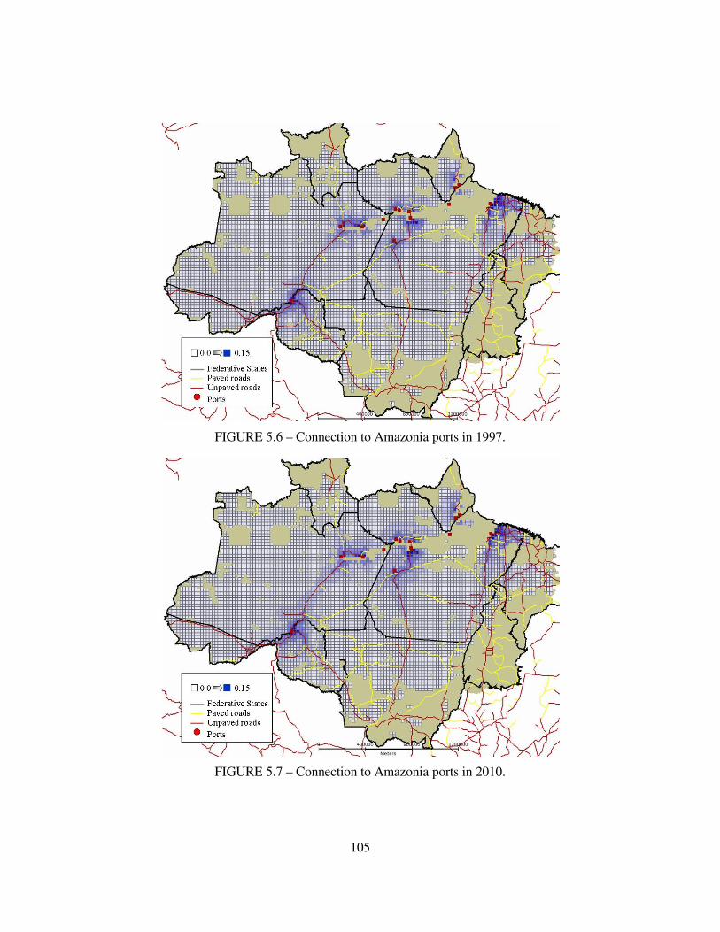
105
FIGURE 5.6 – Connection to Amazonia ports in 1997.
FIGURE 5.7 – Connection to Amazonia ports in 2010.

106
5.2.5.4 Law enforcement scenarios
Three alternative scenarios are considered, summarized in Table 5.5:
• No law enforcement. Private reserves continue to be largely disrespected.
Deforestation pace only slows down after 80% of forest cover in each cell has
been removed. This is the scenario considered in most explorations: A, B, C, and
E.
• Private reserves enforcement. An overall increase in the maintenance of private
forest reserves is assumed in this scenario. The premise is that after 50% of
original forest has been removed in each cell, deforestation pace slows down,
due to law enforcement practices. This scenario is analyzed in Exploration D.
• Local command and control: In certain high pressure areas, command and
control actions take place. In these controlled areas, two premises are adopted:
(a) private forest reserves are more respected; (b) illegal land appropriation
practices are inhibited, slowing the deforestation process. This scenario can also
be seen as the presence of the State, or a “governance” level, non-uniformly
distributed across the region. Outside the controlled areas, allocation parameters
represent the current low level of law enforcement in the Amazonia, as Table 5.5
this scenario is also analyzed in Exploration D.
TABLE 5.5 – Law enforcement scenario parameters.
Forest cover threshold (forest_ threshold)
Maximum allowed change (change_max_lim)
No law enforcement 20% 50% Private Reserve partial enforcement 50% 50% Local Command and Control:
Controlled areas 50% 20% Outside controlled areas 20% 50%

107
5.3 Results and discussion
This section compares the results of the five explorations using maps of hot spots of
change in the forest cover from 1997 to 2020 resulting from the CLUE application.
Besides the visual comparison of the hot-spot maps, selected sites are used to assess
quantitatively the intra-regional differences in the results. Figure 5.8 illustrates these
sites. This quantitative assessment analyzes results inside and outside of protected areas
separately. Thirteen sites are used outside protected areas, distributed in the new
frontiers and more consolidated areas, as Table 5.6 shows. Table 5.7 describes the sites
selected inside protected areas. The two areas in the Central macro-region are only
created in 2004 in the paving and protecting allocation scenario.
FIGURE 5.8 – Sites for quantitative comparison of results.

108
TABLE 5.6 – Sites for quantitative assessments of intra-regional differences outside protected areas.
TABLE 5.7 – Sites for quantitative assessments of intra-regional differences inside protected areas.
Site number Site name Macro-region State
1 Terra do Meio Central Pará
2 Sul do Amazonas Central Amazonas
3 Xingu IL Arch Mato Grosso
4 MT Arch Mato Grosso
Sites outside protected area have the same size (15.000 km2, containing 24 cells of
25x25 km 2). The comparison indicator in this case is percentage of the overall change
allocated in each test site (change in deforestation from 1997 to 2020 in the test site
divided by change in the whole Amazon). Minimum value of the indicator is 0%, and
maximum value is 2.5% (in the baseline demand scenario, this maximum value
Site number Site name Description/Location Macro-region State
1 São Felix/Iriri New frontier - São Felix/Iriri Central Pará
2 BR 163 - South New frontier – Cuiaba-Santarém (South of Novo Progresso) Central Pará
3 BR 163 - North New frontier - Cuiaba-Santarém (North of Novo Progresso) Central Pará
4 BR 163/BR 230 New frontier - Cuiaba-Santarém Central Pará
5 BR 230 - Ruropólis/Trairão Traditional occupation area Central Pará
6 BR 230 - Apuí New frontier - South of Amazonas Central Amazonas
7 BR 319 - Humaitá New frontier - South of Amazonas Central Amazonas
8 BR 319 - Manicoré New frontier - South of Amazonas Central Amazonas
9 BR 319 - Manaus Traditional occupation area Central Amazonas
10 Marabá Traditional occupation area Arch Pará
11 Cumaru/São Felix Unoccupied area in Southern Pará Arch Pará
12 Terra Nova do Norte Traditional occupation area Arch Mato Grosso
13 Aripuanã Unoccupied area in Northern Mato Grosso Arch Mato Grosso

109
corresponds to a deforestation of 12.500 km inside the test site in the period, i.e., 83%
of change). Although absolute values and range of the indicators are small, relative
differences among sites are clear. The goal of the comparison is to use better assess
which areas gained preference over others in the allocation procedure in each
exploration. For the test sites inside protected areas, as their sizes vary, the percentage
of total area deforested in 2020 is use as the comparison indicator.
5.3.1 Exploration A – Analysis of alternative factors: accessibility
This exploration compares the effects of using alternative regression models to assess
the relative importance of different accessibility factors. We employ the
amazon_roads_100 model at coarse resolution, and compare the spatial patterns derived
from using different models at the fine scale. The focus is especially in the Central
macro-zone, where the new Amazonia frontiers are located (Section 2.3). This
exploration compares the use of the amazon25, arch25 and central25 regression
models. Table 5.8 compares the three most significant regression coefficients in each
model. Regarding accessibility factors, the models differ as follows:
• In the amazon25 model, only distance to roads is one of the three most
significant variables. Connection to ports and distance to rivers are also
significant in the model. Connection to markets was not included in this model
due to the high correlation to distance to roads (see Table 5.2).
• In the arch25 model, connection to markets and distance to roads are considered,
and connection to market presents greater importance than distance to roads.
• In the central25 model, connection to ports and distance to rivers are more
important than connection to markets. Distance to roads is the most significant
variable.
This exploration uses the baseline demand scenario, the no change allocation scenario,
and the no law enforcement scenario.

110
TABLE 5.8 - Three most important deforestation determining factors in terms of standardized betas. Variables are listed in order of importance. Plus or
minus signal indicate a positive or negative impact on increasing or decreasing deforestation.
Coarse scale models
amazon_roads100 amazon_urban100
Distance to roads
- Distance to urban centres
-
Humid climate
- Number of settled families
+
Fertile soils
+ Humid climate -
Fine scale models amazon25 arch25 central25 occidental25
Distance to roads: Paved
Unpaved
- -
Protected areas - Distance to roads - Distance to urban centers
-
Protected areas
- Connection to markets
+ Connection to ports + Distance to roads -
Humid climate - Distance to roads: Paved
Unpaved
- -
Distance to rivers - Distance to rivers -
Figures 5.9 to 5.11 show alternative forest change patterns from 1997 to 2020 (hot spots
of change) resulting from the three CLUE model runs. Figure 5.9 shows the resulting
hot-spots of change of using the amazon25 in all spatial partitions. Figure 5.9.b shows
the results of different models for each spatial partition (arch25, central25 and
occidental25). Figure 5.9.c shows the outcome of use of the arch25 model in all spatial
partitions. Figure 5.13 presents a quantitative comparison for some of the test sites.
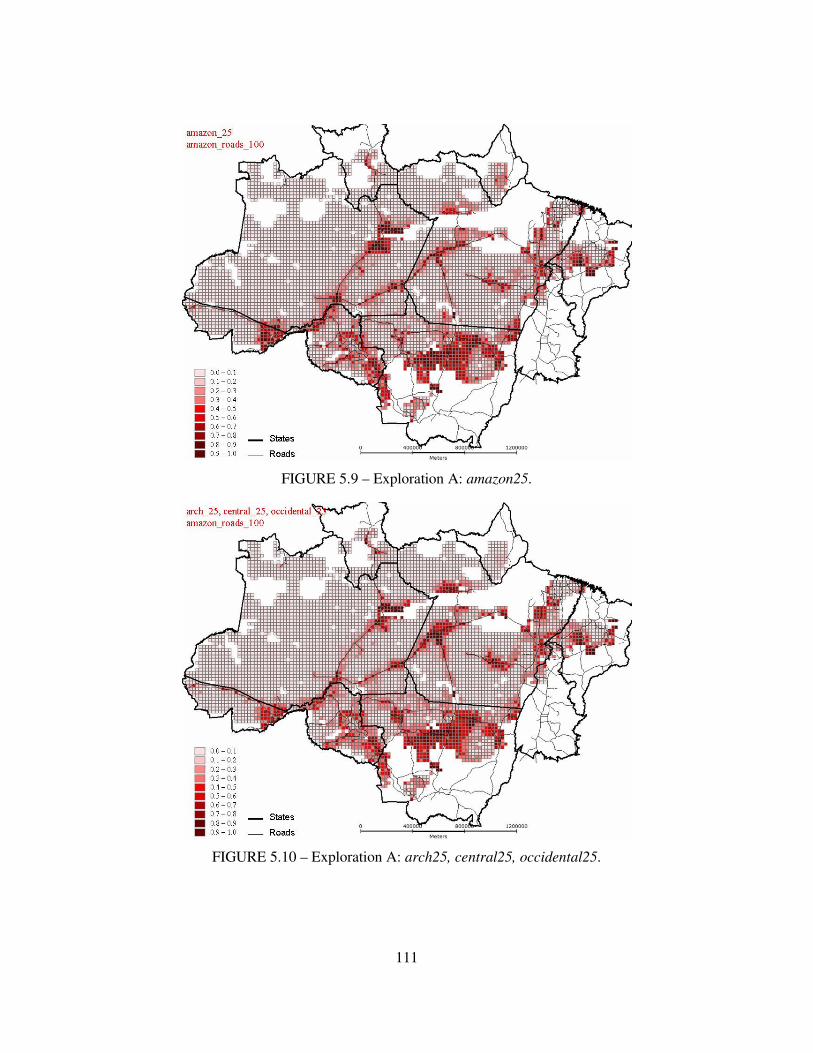
111
FIGURE 5.9 – Exploration A: amazon25.
FIGURE 5.10 – Exploration A: arch25, central25, occidental25.

112

113
FIGURE 5.11 – Exploration A and B: arch25, amazon_roads_100.
FIGURE 5.12 – Exploration B: arch25, amazon_urban_100.

114

115
Exploration A
0.00%
0.50%
1.00%
1.50%
2.00%
2.50%
tota
l ch
%
%
BR 319 - Manaus
BR 163 - South
BR 230 - Ruropólis/Trairão
Sáo Felix/Iriri
BR 319 - Humaitá
BR 319 - Manicoré
BR 230 - Apuí
BR 319 - Manaus 1.81% 1.94% 2.09%
BR 163 - South 1.79% 0.79% 0.86%
BR 230 - Ruropólis/Trairão 1.58% 1.75% 1.37%
Sáo Felix/Iriri 1.38% 1.16% 0.97%
BR 319 - Humaitá 1.37% 0.93% 1.30%
BR 319 - Manicoré 0.87% 0.67% 0.93%
BR 230 - Apuí 0.85% 0.83% 1.05%
arch_25 central_25 amazon_25
FIGURE 5.13 – Exploration A: quantitative comparison among selected test sites.
When the amazon25 model is used (Figure 5.9), resulting patterns at the Central macro-
region tend to concentrate around the Amazon river and ports, and distribute unevenly
along existing roads, with a dominance in the Porto Velho-Manaus road (BR 319).
When the central25 models is used in the Central area (Figure 5.10), resulting patterns
tend to concentrate even more around the Amazon river and close to ports, due to the
importance of connection to ports and distance to rivers in this model. These two
models do not capture the dynamics of the Amazonian new frontiers appropriately.
Currently active areas, such as the Cuiabá-Santarém show a less marked pattern than the
PortoVelho-Manaus, for instance, where the process is starting only now. The pressure
in São Felix/Iriri is also not captured in both models.
Using the arch25 model in all regions (Figure 10.c) captures the different temporal
stage of occupation among different new frontiers, with a stronger process both in the
Cuiabá-Santarém and São-Felix/Iriri areas (see comparison in Figure 5.13). Resulting
patterns reflect the importance of the connectivity to national markets (São Paulo and

116
Northeast) to explain the higher pressure in these areas. This heterogeneity (in space and
time) could not be captured using only measures of distance to roads.
Based on these results, the arch25 model is used as the fine resolution model for the
other explorations presented below. This does not mean an assumption that the process
that happened in the Arch is going to be repeated in the other areas. Instead, the
assumption is that the arch25 model better captures the current and possible axes of
development presented in Section 2.4, especially due to the inclusion of the connection
to markets variable. The arch25 model presents another advantage for scenario
building: protected areas have a higher importance in comparison to the other models,
increasing their effectiveness as a deterrent to the deforestation process. The arch25
model also includes important variables such as distance to timber production areas and
percentage of fertile soils.
In the arch_25 model, climate variables are not used. This may also explain the
difference among the amazon25, central 25, and arch_25 results in the Central macro-
region. The amazon25 and central25 include climate conditions as important deterrents
of occupation, and this may reinforce the concentrated patterns around the Amazon
river in both models (see climate condition variables in Figures 3.22 3.23). Connection
to markets and climate conditions are highly correlated in the Arch and in the whole
Amazonia, and could not be placed in the same regression models. Chapter 4 discusses
the importance of such variables in the occupation process of Amazonia, and concludes
that the diffusive nature of deforestation, distance to roads and to urban centres, climate
and connection to markets, and the interaction among them, contributed significantly
for the pattern of deforestation in 1996/1997. In the following explorations, connection
to markets is used in the fine resolution (arch25 model). Climate conditions influence is
maintained in the large scale, through both coarse resolution models (amazon_roads100
and amazon_urban100), as shown in Table 5.8. In this way, we use the CLUE model
multi-scale approach to incorporate the complementary influence of important and
correlated variables. The multi-scale approach is also explored in relation to other pair
of highly correlated variables, distance to roads and distance to urban centres, as
discussed in the next Exploration.

117
5.3.2 Exploration B – Analysis of alternative factors: local markets
This exploration analyzes the effects of including distance to urban centres in the coarse
resolution model. Distance to urban centres is a proxy of the accessibility to local
markets. The aim of exploration B is to explore how the local markets contribute to the
new frontiers, and to assess the difference between the large-scale influence of the
distance to roads and that of the distance to urban centres.
Exploration B uses the arch25 model in the fine resolution, and compares the use of the
distance to roads model (amazon_roads100) with the distance to urban centres model
(amazon_urban100), in the coarse resolution. Table 5.8 compares the three most
significant regression coefficients in each model. This exploration uses the baseline
demand scenario, the no change allocation scenario, and the no law enforcement
scenario. The result of the amazon_roads100 model is shown in Figure 5.11, and that of
the amazon_urban100 model is shown in Figure 5.12. Figure 5.14 presents a
quantitative comparison for some of the test sites.

118
Exploration B
0.00%
0.20%
0.40%
0.60%
0.80%
1.00%
1.20%
1.40%
1.60%
1.80%
2.00%
To
tal
ch
%
BR 319 - Manaus
BR 230 - Ruropólis/Trairão
BR 163 - South
BR 163 - North
Sáo Felix/Iriri
BR 230 - Apuí
BR 319 - Humaitá
BR 319 - Manicoré
BR 163/BR 230
BR 319 - Manaus 1.81% 1.81%
BR 230 - Ruropólis/Trairão 1.64% 1.58%
BR 163 - South 1.16% 1.79%
BR 163 - North 0.95% 0.76%
Sáo Felix/Iriri 0.95% 1.38%
BR 230 - Apuí 0.81% 0.85%
BR 319 - Humaitá 0.57% 1.37%
BR 319 - Manicoré 0.46% 0.87%
BR 163/BR 230 0.45% 0.28%
urban_roads100 amazon_roads100
FIGURE 5.14- Exploration B: quantitative comparison among selected test sites.
In the amazon_urban100 model, that includes distance to urban centres in the coarse
resolution, distance to roads loses importance in the overall pattern, and importance of
connection to the rest of the country is reinforced. The incorporation of the distance to
urban centres reinforces the heterogeneity of projected patterns. The model result
concentrates the deforestation in the Cuiabá-Santarém area, especially in the central
portion of the road, and creates a connection to the eastern part of the Transamazônica
road, as shown in Figure 5.12. The area close to the Porto Velho–Manaus road is kept
almost undisturbed, except at its extremes. The Apuí and Nova Aripuanã areas, in the
eastern Transamazônica, are identified as occupation hotspots under both explorations.
The differences between model results illustrated in Figures 11, 12 and 14 are a result of
the interaction between the two scales in the CLUE allocation module (Section 5.2.1).
When the amazon_roads100 model is used at the coarse scale, and arch25 at the fine
scale, distance to roads is emphasized at both scales, and led the allocation process. But,
when the amazon_urban100 is used instead, other factors may be indirectly favoured at

119
the fine scale, as the influence from the coarse scale favours other cells. Another
interesting aspect in Figure 12 is that distance to urban centres has an influence on
resulting patterns, but does not determine them. For instance, the urban centres (see
Figure 3.8) in the south of Amazonas (e.g., Humaitá), or along the western part of the
Transamazônica (e.g., Apuí), do not influence the resulting patterns as much as the
single one in the Cuiabá-Santarém (Novo Progresso), due to the interactions with other
factors, especially connection to markets.
Exploration B does not incorporate the hypothesis of paving for any of the existing
roads in the Central area. Even so, the Cuiabá-Santarém, Apuí, and SãoFelix areas
exhibit strong occupation pressure, under all regression models. The Amazon
riverbanks, close to Santarém and Manaus, also exhibit strong deforestation in all
models.
5.3.3 Exploration C - Policy analysis: paving and protected areas
This exploration considers the impact of public policies on projected deforestation
hotspots. This analysis complements explorations A and B, by assessing the relative
importance of different factors when new infra-structure and protected areas are created.
Exploration C uses the same regression models as Exploration B: the arch_25 model in
at the fine resolution, and compares the use of the amazon_roads_100 and
amazon_urban_100 models at the coarse resolution. This exploration also uses the
baseline demand and the no law enforcement scenarios, but the paving and protection
allocation scenario instead.
Figure 5.15 illustrates the results for the amazon_roads100 and Figure 5.16 illustrates
the results for the amazon_urban100 models. Results should also be compared to
Figures 5.10 and 5.11 respectively, in which the no change allocation scenario is
employed. Figure 5.17 presents a quantitative comparison for some of the test sites
outside protected areas.

120

121
FIGURE 5.15 - Exploration C – Paving and Protecting allocation scenario: arch25,
amazon_roads100.
FIGURE 5.16 - Exploration C – Paving and Protecting allocation scenario: arch25,
amazon_urban100.

122

123
Exploration C - amazon_roads100
-0.50%
0.00%
0.50%
1.00%
1.50%
2.00%
No_change
Paving and Protecting
Difference
No_change 1.38% 1.58% 0.87% 0.76% 0.28% 1.79% 1.37% 0.85% 1.81%
Paving and Protecting 1.85% 1.88% 1.12% 1.01% 0.40% 1.88% 1.37% 0.64% 1.56%
Difference 0.47% 0.29% 0.25% 0.25% 0.12% 0.09% 0.00% -0.21% -0.25%
Sáo
Felix/Iriri
BR 230 -
Ruropóli
s/Trairão
BR 319 -
Manicor
é
BR 163 -
North
BR
163/BR
230
BR 163 -
South
BR 319 -
Humaitá
BR 230 -
Apuí
BR 319 -
Manaus
Exploration C - amazon_urban100
-0.50%
0.00%
0.50%
1.00%
1.50%
2.00%
No_change
Paving and Protecting
Difference
No_change 1.64% 0.95% 0.45% 0.95% 1.16% 0.46% 0.57% 0.81% 1.81%
Paving and Protecting 1.89% 1.17% 0.63% 1.12% 1.29% 0.56% 0.52% 0.69% 1.64%
Difference 0.25% 0.22% 0.17% 0.17% 0.13% 0.10% -0.05% -0.11% -0.17%
BR 230 -
Ruropóli
s/Trairão
Sáo
Felix/Iriri
BR
163/BR
230
BR 163 -
North
BR 163 -
South
BR 319 -
Manicor
é
BR 319 -
Humaitá
BR 230 -
Apuí
BR 319 -
Manaus
FIGURE 5.17 - Exploration C: quantitative comparison among selected test sites (outside protected areas)
As Figure 5.17 illustrates, results show heterogeneous impacts of these policies in
different areas. In both models, road paving has a larger impact in the Cuiabá-Santarém
road in comparison to the Porto Velho-Manaus road.
In the Porto Velho-Manaus road, when the amazon_road100 model is used, the road
paving brings a greater overall impact that in the amazon_urban100. The latter model
tends to concentrate deforestation in the extremes of the Porto Velho-Manaus road. This

124
difference is explained by increased importance of the connection to cities and ports in
the amazon_urban100 model. Besides, as discussed in the last section, when combining
different models in different scales, distance to roads loses importance in the overall
pattern, and importance of connection to the rest of the country is reinforced.
Considering the occupation history of the region, and the fact that the Porto Velho-
Manaus road traverses a remote region, without any cities of significant sizes, and the
results of the amazon_urban100 model seems more appropriated than the
amazon_roads100 model for experiment C. However, the arch25 model used in the
fine resolution does not emphasize the connection to ports variable influence in this
region. If a modified model were used in the fine resolution giving more importance to
connection to ports than in the current arch_25 model (which reinforces connection to
national markets) a stronger deforestation pressure would possibly result in the Porto
Velho Manaus. Figure 5.6 and 5.7 show the temporal evolution of the connection to
ports variable when the roads are paved. These effects of paving are stronger in the
Porto Velho-Manaus area. This indicates that the dynamics in this region differs from
the other new frontiers (e.g, SãoFelix, for instance), given its specific connectivity and
also biophysical conditions (see Figures 3.20 3.21 3.22 3.23), so uniform projections
based on the same factors may be misleading.
The results of Exploration C indicate a migration of the deforestation from one area to
another, since the regional demand for land is kept constant. Compared to Exploration B
(where roads are not paved), results show that deforestation increases in cells closer to
the newly paved roads, and decreases in non-paved roads. For example, deforestation
decreases in the Apuí region, in the Eastern part of Transamazônica road, which is not
paved in Exploration C. The same holds for protected areas: where new protected areas
are created, the occupation process slows down (see also Figure 5.29). But, as demand
is kept constant, creation of protected areas induces the migration of deforestation to
other areas. For instance, the deforestation in the Terra do Meio decreases due to the
creation of protected areas, but it compensated by an increase in other areas, such as the
western side of the Cuiabá-Santarém road.

125
Although the spatial interactions seen in the model results are a direct consequence of
our premises regarding demand (demand for land is fixed, so it will be allocated
somewhere by the model), they are useful as they clearly illustrate how these
interactions may occur. Results illustrate how the local policies effects may be felt in
other areas, not necessarily in a beneficial way, according to the actor’s perceptions of
new constraints and opportunities created by policies. They also facilitate the
envisioning of how the productive system that generates such demand can influence the
occupation process. The productive system (e.g., the soybean market chain, the beef
market chain) act in several spatial and temporal scales; in the medium and long run it
may reorganize, and contribute to the occupation of new locations to attend a growing
demand for agricultural products. Intensification would be another possible reaction to
policy imposed constraints in the access to land (especially in the case of an overall
decrease in land availability), and this is not treated in our current model. The results of
Exploration C indicate that these intra-regional interactions must be taken into account
for public policy making, and that understanding these market chains is essential to the
design of effective policies for the Amazonia.
5.3.4 Exploration D - Policy analysis: law enforcement
Exploration D consists of analyzing the results of two law enforcement scenarios
presented in Table 5.5: the Private Reserves Enforcement and the Local Command and
Control scenarios. In this exploration, we use the same models as Exploration A (the
amazon_roads100 model at coarse resolution and the arch25 model at fine resolution),
the baseline demand scenario and the no change allocation scenario. Figure 5.18 present
the results of the “Private Reserves” law enforcement scenario. Figure 5.20 illustrates
the controlled areas used “Local Command Control” scenario, on top of Exploration A
results (amazon_roads100, arch_25, No law enforcement scenario). Figure 5.21 shows
the “Local Command Control” scenario results. Figures 5.19 and 5.22 present
quantitative assessments of change in selected test sites the two scenarios.

126

127
FIGURE 5.18 - Exploration D – Private Reserve Partial Law Enforcement scenario: arch25, amazon_urban100
Exploration D - Private reserves enforcement
-0.50%
0.00%
0.50%
1.00%
1.50%
2.00%
tota
l ch
%
No law enforcement
Private reserves partial enforcement
Difference
No law enforcement 1.55% 1.38% 0.39% 0.84%
Private reserves partial
enforcement
1.45% 1.29% 0.48% 1.17%
Difference -0.11% -0.09% 0.09% 0.33%
Terra Nova
do NorteSáo Felix/Iriri
Cumaru/São
FelixAripuanã
FIGURE 5.19 - Exploration D: quantitative comparison among selected test sites in the Private Reserves Partial law enforcement scenario.

128

129
FIGURE 5.20 - Exploration D - No law enforcement scenario: arch25,
amazon_urban100
FIGURE 5.21 - Exploration D - Local Command and Control scenario: arch25,
amazon_urban100

130

131
Exploration D - Local command and Control
-1.00%
-0.50%
0.00%
0.50%
1.00%
1.50%
2.00%
tota
l c
h %
No command and control
Command and control actions
Difference
No command and control 1.79 1.55 1.37 0.84 1.38 0.39 0.76 0.87 1.58 0.85
Command and control actions 1.01 0.92 1.15 0.64 1.36 0.40 0.79 0.91 1.63 0.89
Difference -0.78 -0.63 -0.22 -0.20 -0.02 0.02 0.03 0.05 0.05 0.05
BR
163 -
Sout
h
Terra
Nova
do
Norte
BR
319 -
Hum
aitá
Aripu
anã
Sáo
Felix/
Iriri
Cum
aru/S
ão
Felix
BR
163 -
North
BR
319 -
Mani
coré
BR
230 -
Ruro
pólis/
Trair
BR
230 -
Apuí
FIGURE 5.22 - Exploration D: quantitative comparison among selected test sites in the Command and Control law enforcement scenario.
Exploration D shows the same intra-regional interaction patterns as previous results, as
demand is kept constant. The enforcement of private forest reserves across the region
decreases the change in previously occupied areas, but creates an overall pressure in
other areas (Figures 5.18 and 5.19). Compare Rondônia and the north of Mato Grosso,
for instance, as marked in Figure 5.18. Local command and control actions results
show that localized actions are effective in the areas where they are applied (Figures
3.21 and 3.22), but create a pressure somewhere else. For instance, deforestation
increases in the northern part of Cuiabá-Santarém road when actions are concentrated in
its southern part. These results can be interpreted as a hypothetical “governance level”
heterogeneously distributed in space. They show that localized command and control
actions are not sufficient to reduce deforestation, if the demand is not reduced.
This exploration show interesting results about the Arch macro-region. In the Private
Reserves scenario, there is less saturation (cells 100% deforested), for instance in
Rondônia, but occupation spreads over the whole Arch area. In this scenario, higher
pressure is also felt in the protected areas, specially the ones in areas with higher
connectivity level, as the Xingu Indigenous Land in the Mato Grosso state. Figure 5.29
illustrates these heterogeneous impacts quantitatively.

132
Exploration D - Effect on protected areas of private reserves law
enforcement
0%
5%
10%
15%
20%
25%
30%
35%
No law enforcement
Private reserves partial enforcement
No law enforcement 13% 13% 22% 14%
Private reserves partial
enforcement
13% 15% 29% 21%
Terra do MeioSouth of
Amazonas
Xingu
Indigenous LandMato Grosso
FIGURE 5.23 - Exploration D: quantitative comparison among selected test sites in the Private Reserves Partial law enforcement scenario.
Although this is a very improbable scenario (law enforcement in private reserves but not
in the protected areas), results should be analyzed under another perspective, as a
warning: if demand for land is constant, and private reserves are enforced, occupation
pressure will increase in other areas, including the protected areas. We ran an
alternative simulation, maintaining the same demand level for the Arch, but pushing the
forest threshold to 80%, as would be required by current Brazilian legislation. The
model failed to allocate the demand. These results indicate that occupation level in the
Arch will be reaching a limit in 2020, and reinforce that to preserve the remaining forest
areas in the Arch, in public and private lands, effective and generalized command and
control measures will be necessary. In next section, this aspect is further discussed, as
we present results related to the market constraints on demand for land.
5.3.5 Exploration E: Alternative demand scenarios
Exploration E considers the impact of increasing and decreasing the demand,
representing the expansion or retraction of market forces that act on the Amazonia. It
uses the paving and protecting allocation scenario. This analysis complements
Exploration C, exploring the potential outcomes of the new infra-structure and protected
areas in alternative market constraint scenarios. As in Exploration C, it uses the arch25

133
model at fine resolution, and compares the results of roads model (amazon_roads100)
and the distance to urban centres model (amazon_urban100) at coarse resolution. Roads
are paved according to the schedule shown in Table 5.4 according to the Paving and
Protecting allocation scenario. The no law enforcement scenario is adopted.
The results for decreasing demand are shown in Figure 5.24 (amazon_roads100 model)
and Figure 5.25 (amazon_urban100 model). The results of increasing demand are
shown in Figure 5.26 (amazon_roads100 model) and Figure 5.27 (the
amazon_urban100). It is useful to compare the results with the results of Exploration C.

134

135
FIGURE 5.24 - Exploration E – Decreasing demand: arch25, amazon_roads100.
FIGURE 5.25 - Exploration E – Decreasing demand: arch25, amazon_urban100.

136
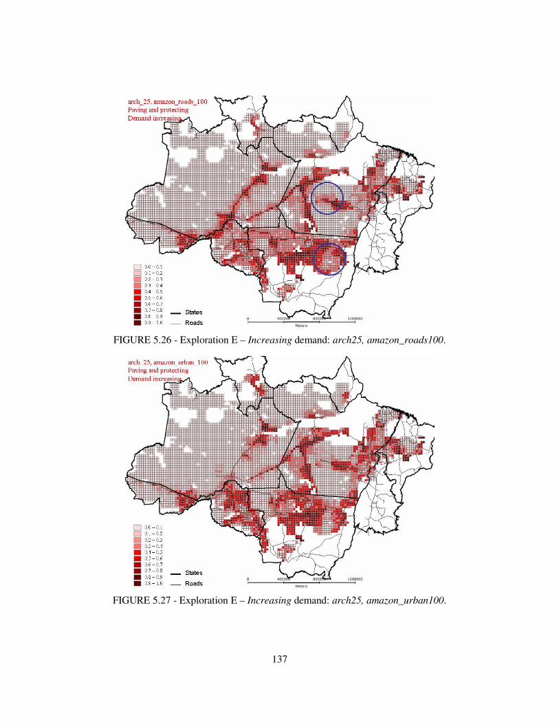
137
FIGURE 5.26 - Exploration E – Increasing demand: arch25, amazon_roads100.
FIGURE 5.27 - Exploration E – Increasing demand: arch25, amazon_urban100.

138

139
Exploration E
0
2000
4000
6000
8000
10000
12000
Increasing Baseline Decreasing
ch
an
ge
(km
2)
BR 319 - Manaus
BR 163 - South
BR 230 - Ruropólis/Trairão
Terra Nova do Norte
Sáo Felix/Iriri
BR 319 - Humaitá
BR 319 - Manicoré
FIGURE 5.28 - Exploration E: quantitative comparison among selected test sites (outside protected areas)
Exploration E - Increased demand effect on protected areas
0%
5%
10%
15%
20%
25%
30%
35%
No-change allocation and Baseline
demand
Paving and protection allocation and
Baseline demand
Paving and protection allocation and
Increased demand
No-change allocation
and Baseline demand
13% 13% 22% 14%
Paving and protection
allocation and Baseline
demand
9% 8% 21% 14%
Paving and protection
allocation and Increased
demand
14% 10% 29% 21%
Terra do
Meio
South of
Amazonas
Xingu
Indigenous
Land
Mato
Grosso
FIGURE 5.29 - Exploration E: quantitative comparison among test sites (inside protected areas).

140
Compared to Exploration C (constant demand), Exploration E results show similar
patterns, both when demand increases and decreases. For increased demand (Figures
5.26 and 5.27), the added quantity of change is not uniformly distributed over the
region, especially in the Central area, as illustrated in as Figure 5.28. In the Cuiabá-
Santarém and São Felix/Iriri the impact is stronger, due to better connectivity
characteristics than other areas. However under any demand scenario (considering the
paving and protection scenario), the following test sites presented the largest changes,
even if the relative order changed: BR163–South, BR230-Ruropólis/Trairão and São
Felix/Iriri in Pará State; BR319–Manaus, BR 319–Humaitá, BR 319–Manicoré in
Amazonas State; and Terra Nova do Norte in Mato Grosso State.
Increased demand also causes a higher pressure on protected areas, in a non-uniform
way, as pointed out in Figures 5.26 and 5.29. This pressure is stronger in the Arch
protected areas (for instance in the Xingu Indigenous Land), but it can also be felt in the
more connected areas in Central region, for instance in Terra do Meio. As Figure 5.29
show, the decrease in the deforestation rate in the Terra do Meio area obtained by the
creation of the protected areas could be lost if the overall demand for land is increased.
Results indicate that the vulnerability of protected areas is non-homogeneous across the
region, and command and control actions should take this into consideration.
In the situation where demand decreases, the stronger impact is felt in the hotspots of
the Central area of Amazonia. The regions along the Cuiaba-Santarém, Porto Velho-
Manaus and western Transamazônica roads show a significant decrease in deforestation
rates. This is a significant result, since it is the only scenario where the crucial Central
region of Amazonia suffers less impact. It indicates that, unless demand for land use is
controlled and reduced in the whole of Amazonia, law enforcement policies and
creation of protected area will have limited overall impact on the deforestation process.

141

142
CHAPTER 6
CONCLUSIONS
6.1 Spatial statistical analysis conclusions
Chapter 4 presented a spatial regression analysis to explore intra-regional differences in
the relative importance of land-use determining factors in the Amazon. The analysis
was based on a cellular database including several environmental, socio-economic and
political potential factors, presented in Chapter 3. The results confirm the first
hypothesis explored in this thesis: the relative importance and significance of land use
determining factors greatly vary across the Amazon. The quantitative results obtained
using this methodology corroborate with the statement of Becker (2001): “in the
Amazon coexist sub-regions with different speed of change, due to the diversity of
ecological, socio-economic, political and of accessibility conditions”. The use of spatial
regression models also corroborated earlier assessments about the diffusive nature of
land-use change in the Amazon (Alves, 2002) as showed by the high values of the
autocorrelation coefficient in all models. Only in the Occidental region values were
slightly lower, indicating a less intense diffusive pattern and speed of change.
The models show the significance of several of the potential determining factors,
demonstrating that focusing on single factor analysis can be misleading. It is the
interaction of many factors that can explain the land-use patterns in the Amazon. And
the relative importance of such factors varies from one region to another, and unravels
the region heterogeneity in terms of patterns and speed of change. For instance, when
only the Arch is analyzed, protected areas becomes the second most important factor,
after the deforestation spatial dependence coefficient, preceding distance to roads and to
urban centers, indicating how they play an important role in avoiding deforestation in
high pressure areas. On the other hand, distance to roads is an important factor in all
space partitions. But the multi-factor analysis shows that the heterogeneous occupation
patterns of the Amazon can only be explained when combining roads to other factors

143
related to the organization of the productive systems in different regions, such as
favourable environmental conditions and access to local and national markets. This
provides further evidence that the implantation of roads and development poles in the
70s was a first incentive to deforestation, but it continued more elevated in regions that
established productive systems linked to the Center, South and Northeast of Brazil
(Alves, 2001; Alves, 2002).
The municipality of São Felix do Xingu, a current deforestation hot-spot, is exemplary
of this: it has been the lead in deforestation rates in the last years (INPE, 2005),
although it is not served by a paved road. Land market plays an important role there,
and also lack of State presence, but it also has a very well organized beef market chain
(Escada et al., 2005a). The agrarian structure and specific land-use analysis results
reinforce the conclusions in relation to the importance of the productive systems, as they
point out the heterogeneity of land use systems adopted by different actors, and the
influence of the agrarian structure on land-use pattern distribution across the region.
Incorporating this heterogeneity of factors, actors, land-use and productive systems is
essential to a sound understanding of the land-use change process in the region,
especially to subside policy decisions appropriated for each sub-region in a non-uniform
and non-misleading way.
6.2 Dynamic modeling conclusions
Chapter 5 presented the results of a modified version of the CLUE modeling framework
to explore scenarios of land use change in the Brazilian Amazonia. The concept of
“scenario exploration” was introduced. Each exploration emphasized a different aspect
of the Amazonia occupation process. Out of many possibilities, this work presented the
results of five explorations which analyze the effects of alternative accessibility factors,
policies and market constraints.
Three main conclusions can be drawn from the results. First, connection to national
markets is the most important factor for capturing the spatial patterns and different stage
of occupation of the new Amazonian frontiers. Second, it is the interaction between
connectivity and other factors, which may act in different scales (such as climate and

144
proximity to local markets) that influence the intra-regional dynamics, and creates
differentiated local conditions in the new expansion axes. Such patterns cannot be
explained by single factor that focus on the role of roads, for instance. And third, these
intra-regional differences led to heterogeneous impact of policies across the region.
These three conclusions corroborate with this thesis hypotheses, about the heterogeneity
of land use determining factors and the importance of connection to markets in the
occupation process.
Results also point out that public policies for the Amazonia must take into consideration
the spatial and temporal interaction between localized policies and regional processes.
Our models do not incorporate any assumptions regarding how policies affect
(positively or negatively) the overall deforestation rates. Instead, we analyzed the
patterns emerging from changing three constraints separately: (a) infra-structure; (b) law
enforcement and conservation policies; and (c) market forces. The interaction among
these three constraints is not well understood at this moment. Results illustrate how the
local policies effects may be felt in other areas, not necessarily in a beneficial way,
according to the actor’s perceptions of new constraints and opportunities created by
policies. Besides, the productive system acts in several spatial and temporal scales. In
the medium and long run, market chains may reorganize, according to the constraints
imposed by policy action, and contribute to the occupation of new areas to attend a
growing demand for agricultural products Such processes and interactions happen at
different hierarchical levels, so multi-scale and multi-localities studies are necessary.
The results also indicate that, in complex regions such as Amazonia, scenario
exploration is a powerful tool for comparing the results of land use models. Given the
inbuilt uncertainties of LUCC model, controlled scenarios where one key parameter
changes at a time are very useful to gain insight over the occupation process.
6.3 Suggestions for future work
Based on the results and conclusions of this thesis, the suggestions of future work about
the whole Amazonia occupation process are:

145
• Intra-regional interactions in the Amazonia need to be better understood. Future
work should primarily aim at understanding how the balance between public
policies and market constraints, mediated by heterogeneous local conditions,
can affect the future of the Amazonia occupation process. This requires multi-
scale and multi-localities studies, as these processes and interactions happen at
different hierarchical levels.
• Different market chains may influence the occupation process in different ways.
The suggestion is to continue this work by refining the pasture and temporary
agriculture studies, focusing on cattle and soybeans expansion in the Amazonia.
A new IBGE agricultural census is planned for 2006.
• The connectivity measures proposed in this thesis are based on the road network.
Future work should refine these measures, and include river and train transport
networks, in compound measures of connectivity considering the whole
transport network system. Other types of network could also be explored, such
as the telecommunication and urban networks.
• This thesis explores the use of empirical derived relationships combined with
knowledge about the occupation processes. This was achieved mainly by
comparing the effects of alternative regression models on projected patterns. A
step beyond would be to change regression coefficients based on expert
knowledge in controlled explorations. For instance, increasing the importance of
connection to ports in the arch25 model to explore its effects.
• In this work, we introduced a mechanism in the CLUE framework to incorporate
the heterogeneous presence of the State across the region, tested in the law
enforcement scenarios. We used a spatial indicator to refrain or speed up
processes of change on top of (and interacting with) the spatial determining
factors empirically derived. This concept could further explored as a mean of
incorporating other subjective/qualitative indicators not easily derived from
empirical evidence in the modeling framework. For instance, to explore the

146
effectiveness of the presence of IBAMA or INCRA in different regions; the
aspirations of different States towards conservation and development; the level
of social organization of small farmers, indigenous peoples, etc.
• The allocation scenarios built in this thesis were based on the temporal evolution
of the accessibility and protection factors. Allocation scenarios related to other
factors could also be explored, for instance: the creation and growth of urban
centres; the migration of timber production sites; the changes in the agrarian
structure related to the soybeans expansion in the Amazon; the evolution of
technological variables in the Arch related to agricultural intensification, etc.
Finally, we conclude that statistical and dynamic models, when used with knowledge
about the underlying processes, and based on clear premises, can be useful tools to
provide insights about the occupation process of the Amazonia, and properly subside
public policies.

147
BIBLIOGRAPHICAL REFERENCES
Aguiar, A. P. D.; Câmara, G.; Souza, R. C. M., 2003. Modeling Spatial Relations by Generalized Proximity Matrices. In: GeoInfo 2003 - V Brazilian Symposium on Geoinformatics. Campos do Jordao. p.
Akaike, H. A new look at the statistical model identification. IEEE Transactions on Automatic Control, 19 (6): 716- 723, 1974.
Alves, D. S. O Processo de desmatamento na Amazônia. Parcerias Estratégicas (12): 259-275, 2001.
Alves, D. S. Space-time Dynamics of Deforestation in Brazilian Amazônia. International Journal of Remote Sensing, 23 (14): 2.903-2.908, 2002.
Andersen, L.; Granger, C.; Reis, E.; Winhold, D.; Wunder, S., The dynamics of Deforestation and Economic Growth in the Brazilian Amazon. Cambridge: Cambridge University Press, 2002.
Andersen, L.; Reis, E., 1997, Deforestation, development, and government policy in the Brazilian Amazon: an econometric analysis (IPEA Report 76-1997), Rio de Janeiro, IPEA.
Anselin, L., 2001. Spatial Econometrics. In: BALTAGI, B., ed., A Companion to Theoretical Econometrics: Oxford, Basil Blackwell, pp. 310-330.
Arima, E.; Barreto, P.; Brito, M., Pecuária na Amazônia: tendências e implicações para a conservação ambiental. Belém: Instituto do Homem e Meio Ambiente na Amazônia, 2005.
Bailey, T.; Gattrel, A., Spatial Data Analysis by Example. London: Longman, 1995.
Barbier, E. B.; Burgess, J. C. The economics of tropical deforestation. Journal of Economic Surveys, 15 (3): 413-433, 2001.
Becker, B., Amazönia. Ática, 1997.
Becker, B., Amazônia: geopolítica na virada do III milênio (Amazônia: geopolitics in the turn of the third millenium). Rio de Janeiro: Garamnd. 172 pp, 2004.
Becker, B. Cenários de Curto Prazo para o Desenvolvimento da Amazônia. Cadernos IPPUR, Ano XIV (1), 2000.
Becker, B. Geopolítica da Amazônia (Amazonian Geopolitics). Estudos Avancados (Journal of the Institute of Advanced Studies of the University of Sao Paulo) - Dossiê Amazônia Brasileira I, 19 (53): 71-86, 2005.

148
Becker, B. Revisão das Políticas de Ocupação da Amazônia: é possível identificar modelos para projetar cenários? (Revision of Amazon occupation policies: it is possible to identify models for scenario building?). Parcerias Estrategicas, 12: 135-159, 2001.
Brasil. Plano de Ação para a prevenção e controle do desmatamento na Amazônia Legal - Grupo Permanente de Trabalho interministerial para a redução dos índices de desmatamento da Amazônia Legal 2004.www.presidencia.gov.br/casacivil/desmat.pdf.
Brasil. Tendências Desmatamento 2004/2005 - Plano de Ação para Prevenção e Controle do Desmatamento na Amazônia. 2005.http://www.mma.gov.br/doc/tendencias_desmatamento2004_2005.pdf.
Briassoulis, H., 2000, Analysis of Land Use Change: Theoretical and Modeling Approaches, Regional Research Institute, West Virginia University
Brito, M. S. Políticas Públicas e Padröes de Uso da Terra na Amazönia Legal. Revista Brasileira de Geografia, 57 (3): 73-93, 1995.
Brown, K.; Pearce, D., The causes of tropical deforestation, the economic and statistical analysis of factors giving rise to the loss of tropical forests. London: University College London Press, 1994.
Costa, W. M., O Estado e as Políticas Territoriais no Brasil. Contexto, 1997.
Costanza, R.; Ruth, M. Using Dynamic Modeling to Scope Environmental Problems and Build Consensus. Environemental Management, 22: 183-195, 1998.
De Koning, G. H. J.; Verburg, P.; Veldkamp, A.; Fresco, L. O. Multi-scale modeling of land use change dynamics in Ecuador. Agricultutal Systems: 77-93, 1999.
Escada, M. I.; Vieira, I. C.; Kampel, S.; Araújo, R.; Veiga, J. B.; Aguiar, A. P. D.; Veiga, I.; Oliveira, M.; Pereira, J. G.; Carneiro, A.; Fearnside, F. M.; Venturieri, A.; Carriello, F.; Thales, M.; Carneiro, T. S.; Monteiro, A. M.; Câmara, C. Processos de ocupação nas novas fronteiras da Amazônia (o interflúvio do Xingu/ Iriri) (Occupation process in the new frontiers of the Amazon (the Xingu/Iriri region)
Estudos Avancados (Journal of the Institute of Advanced Studies of the University of Sao Paulo) - Dossiê Amazônia Brasileira II, 19 (54): 9-24, 2005a.
Escada, M. I. S.; Aguiar, A. P. D.; Monteiro, A. M. V. O Avanço do Desmatamento na Amazônia no Contexto das Novas Fronteiras (The deforestation process in Amazönia in the context of the new frontiers). 2005b.http://www.obt.inpe.br/prodes/seminario2005/.
Faminow, M. Spatial economics of local demand for cattle products in Amazon development. Agriculture, Ecosystems & Environment, 62 (1): 1-11, 1997.
Fearnside, F. M. Soybean cultivation as a threat to the environment in Brazil. Environemental Conservation, 28 (1): 23-38, 2001.

149
Fearnside, P. Deforestation in Brazilian Amazon: the effect of population and land tenure. Ambio, 8: 537-545, 1993.
Ferreira, V. L. V., E., Almeida, S. . O desmatamento na Amazônia e a importância das áreas protegidas (Amazon deforestation and the importance of protected areas). Estudos Avancados (Journal of the Institute of Advanced Studies of the University of Sao Paulo) - Dossiê Amazônia Brasileira I, 19 (53): 157-166., 2005.
Geist, H.; Lambin, E. F., 2001, What Drives Tropical Deforestation?A meta-analysis of proximate and underlying causes of deforestation based on subnational case study evidence, in OFFICE, L. I. P., ed., LUCC Report Series No. 4.
Geoma, 2003, Dinâmica Territorial e sócio-ambiental nas frentes de ocupação e áreas consolidadas: os casos deSão Felix do Xingu-Iriri e da região de Marabá, Relatório do Seminário de Marabá, Ministério da Ciência e Tecnologia.
Gibson, C.; Ostrom, E.; Ahn, T. K. The concept of scale and the human dimensions of global change: a survey. Ecological Economics, 32: 217–239, 2000.
Ibge, 1996, Censo Agropecuario 1996 (Agricultural Census 1996), Instituto Brasileiro de Geographia e Estatistica (Brazilian Census Bureau).
Ibge, 2000, Censo Demografico 2000 (Demographical Census 2000), Instituto Brasileiro de Geographia e Estatistica (Brazilian Census Bureau).
Ibge, 2006a, Pesquisa Agrícola Municipal (Municipal Agricultural Research), Instituto Brasileiro de Geographia e Estatistica (Brazilian Census Bureau).
Ibge, 2006b, Pesquisa Pecuária Municipal Instituto Brasileiro de Geographia e Estatistica (Brazilian Census Bureau).
Inpe. Monitoramento da Floresta Amazônica Brasileira por Satélite (Monitoring the Brazilian Amazon Forest by Satellite). São José dos Campos, Brazil: Instituto Nacional de Pesquisas Espaciais (National Institute for Space Research), 2005.http://www.obt.inpe.br/prodes/.
Irwin, E.; Geoghegan, J. Irwin, E., Geoghegan, J. Theory, data, methods: developing spatially-explicit economic models of land use change. Agric. Ecosyst. Environ. 85, 7–24, 2001. Agriciculture, Ecosystems and Environonment, 85: 7–24, 2001.
Kaimowitz, D., Angelsen, A., Economic Models of Tropical Deforestation: A Review. Bogor, Indonesia: Center for International Forestry Research (CIFOR) 1998.
Kirby, K. R.; Laurance, W. F.; Albernaz, A. K.; Schroth, G.; Fearnside, P. M.; Bergen, S.; Venticinque, E. M.; Costa, C. D. The future of deforestation in the Brazilian Amazon. Futures, in press, 2006.

150
Kok, K.; Farrow, A.; Veldkamp, A.; Verburg, P. H. A method and application of multi-scale validation in spatial land use models. Agriculture, Ecosystems and Environment, 85: 223-238, 2001.
Kok, K.; Veldkamp, A. Evaluating impact of spatial scales on land use pattern analysis in Central America. . Agriciculture, Ecosystems and Environonment, 85: 205–221, 2001.
Lambin, E. Modeling and Monitoring land-cover change processes in tropical regions. Progress in Physical Geography 21 (3): 375-393, 1997.
Lambin, E.; Geist, H. J. Regional Differences in Tropical Deforestation. Environemt, 45 (6): 22-36, 2003.
Lambin, E.; Rounsevell, M. D. A.; Geist, H. J. Are agricultural land-use models able to predict changes in land-use intensity? Agriculture, Ecosystems and Environment, 82: 321–331, 2000.
Lambin, E. F.; Geist, H. J. "Global land-use and cover change: What have we learned so far?" Global Change Newsletter, 46, 2001.
Lambin, E. F.; Turner, B. L. I.; Geist, H. J.; Agbola, S. B.; Angelsen, A.; Bruce; J.W.; Coomes, O.; Dirzo, R.; Fischer, G.; Folke, C.; George, P. S.; Homewodd, K.; Imbernon, J.; Leemans, R.; Li, X.; Moran, E. F.; Mortimore, M.; Ramakrishnan, P. S.; Richards, J. F.; Skånes, H.; Steffen, W.; Stone, G. D.; Svedin, U.; Veldkamp, T. A.; Vogel, C.; Xu, J. The Causes of Land-Use and Land-Cover Change. Moving Beyond the Myths. Global Environmental Change:Human and Policy Dimensions, 4, 2001.
Laurance, W.; Albernaz, A. K.; Schroth, G.; Fearnside, P. M.; Bergen, S.; Venticinque, E.; Dacosta, C. Predictors of deforestation in the Brazilian Amazon. Journal of Biogeography, 29: 737-748, 2002.
Laurance, W.; Cochrane, M.; Bergen, S.; Fearnside, P.; Delamonica, P.; Barber, C.; D'angelo, S.; Fernandes, T. The future of the Brazilian Amazon. Science, 291: 438-439, 2001.
Lentini, M.; Veríssimo, A.; Pereira, D. The expansion of logging in the Brazilian Amazon. State of the Amazon, 2, 2005.
Machado, L., 1998. A fronteira agrícola na Amazônia. . In: BECKER, B. K.; CHRISTOFOLETTI, A.; DAVIDOCH, F. R.; GEIGER, R. P. P., eds., Geografia e meio ambiente no Brasil, pp. 181-217.
Margulis, S., 2004, Causes of deforestation in Brazilian Amazon (World Bank Working Paper 22), Washington, World Bank.
Mertens, B.; Poccard-Chapuis, R.; Piketty, M. G.; Lacques, A. E.; Venturieri, A. Crossing spatial analyses and livestock economics to understand deforestation process

151
in the Brazilian Amazon: the case of São Felix do Xingu in South Pará. Agricultural Economics, 27: 269-294, 2002.
Nepstad, D.; Carvalho, G.; Barros, A. C.; Alencar, A.; Capobianco, J. P.; Bishop, J.; Moutinho, P.; Lefebvre, P.; Silva-Jr., U. L.; Prins, E. Road Paving, fire regime feedbacks, and the future of Amazon Forests. Forest Ecology and Managment, 154: 395-407, 2001.
Nepstad, D.; Verissimo, A.; Alencar, A.; Nobre, C.; Lima, E.; Lefebvre, P.; Schlesinger, P.; Potter, C.; Moutinho, P.; Mendoza, E. Large-scale impoverishment of Amazonian forests by logging and fire. Nature, 6727: 505-507, 1999.
Overmars, K. P.; Koning, G. H. J. D.; Veldkamp, A. Spatial autocorrelation in multi-scale land use models. Ecological Modeling, 164: 257-270, 2003.
Parker, D. C.; Berger, T.; Manson, S.; Mcconnel, S., 2001. Report and Review of the International Workshop. In: Agent-Based Models of Land-Use /Land-Cover Change.LUCC Report Series no 6. Irvine, California, USA. p.
Perz, S. G.; Skole, D. L. Social determinants of secondary forests in the Brazilian Amazon. Social Science Research, 32: 25-60, 2003.
Pfaff, A. What drives deforestation in the Brazilian Amazon? Evidence from Satellite and Socio-economic data. Journal of Environmental Economics and Management, 37: 26-43, 1999.
Poccard-Chapuis, R. Les réseaux de la conquête. Filières bovines et structuration de l’espace sur les fronts pionniers d’Amazonie Orientale brésilienne.Paris: Paris, 2004.Géographie, 2004.
Reis, E.; Guzmán, R., 1994. An econometric model of Amazon Deforestation. In: BROWN, K.; PEARCE, D., eds., The causes of tropical deforestation, the economic and statistical analysis of factors giving rise to the loss of tropical forests: London, University College London Press, pp. 172-91.
Reis, E.; Margulis, S., 1991. Options for slowing Amazon jungle clearing. In: DORNBUSCH, R.; POTERBA, J. M., eds., Global Warming: economic policy responses: Cambridge, Massachusetts, MIT Press, pp. 335-80.
Ribeiro, B., Veríssimo, A., Pereira, K., 2005, O Avanço do Desmatamento sobre as Áreas Protegidas em Rondônia, O Estado da Amazônia, Imazon.
Santilli, M.; Moutinho, P.; Schwartzman, S.; Nespstad, D.; Curran, L.; Nobre, C. Tropical Deforestation and the Kyoto Protocol: an editorial essay Climate Change, 71: 267-276, 2005.

152
Schneider, R. R., Arima, E., Veríssimo, A., Barreto, P., Souza, Jr, 2000, Amazônia Sustentável: limitantes e oportunidades para o desenvolvimento rural., in IMAZON, W. B. A., ed., Série Parcerias.
Soares-Filho, B.; Cerqueira, G.; Pennachin, C. DINAMICA – a stochastic cellular automata model designed to simulate the landscape dynamics in an Amazonian colonization frontier. Ecological Modeling, 154 (3): 217 – 235, 2002.
Soares-Filho, B.; Nepstad, D.; Curran, L.; Cerqueira, G.; Garcia, R.; Ramos, C. A.; Voll, E.; Mcdonald, A.; Lefebvre, P.; Schlessinger, P. Modeling conservation in the Amazon basin. Nature, 4389, 2006.
Thery, H. Situações da Amazônia no Brasil e no continente (Amazonia situation in Brazil and in the continent). Estudos Avancados (Journal of the Institute of Advanced Studies of the University of Sao Paulo) - Dossiê Amazônia Brasileira I, 19 (53): 37-49, 2005.
Veldkamp, A.; Fresco, L. CLUE-CR: an integrated multi-scale model to simulate land use change scenarios in Costa Rica. Ecological Modeling, 91: 231-248, 1996.
Veldkamp, A.; Lambin, E. Predicting land-use change. A. Veldkamp a,∗, E.F. Lambinb,, 85: 1-6, 2001.
Veldkamp, A.; Verburg, P.; Kok, K.; De Koning, G.; Priess, J.; Bergsma, A. The need for scale sensitive approached in spatially explicit land use change modeling. . Environmental Modeling and Assessment, 6: 111-121, 2001.
Verburg, P.; De Koning, G.; Kok, K.; Veldkamp, A.; Bouma, J. A spatial explicit allocation procedure for modeling the pattern of land use change based upon actual land use. Ecological Modeling, 116: 45-61, 1999a.
Verburg, P.; Veldkamp, A. The role of spatially explicit models in land-use change research: a case study for cropping patterns in China. Agriculture, Ecosystems and Environment, 85: 177–190, 2001.
Verburg, P.; Veldkamp, A.; Fresco, L. O. Simulation of changes in the spatial pattern of land use in China. Applied Geography, 19 211–233, 1999b.
Verburg, P. H.; Schot, P. P.; Dijst, M. J.; Veldkamp, A. Land use change modeling: current practice and research priorities. GeoJournal, 61 (4): 309-324, 2004.
Walker, R. T.; Moran, E.; Anselin, L. Deforestation and Cattle Ranching in the Brazilian Amazon: External Capital and Household Processes. World Development, 28 (4): 683-69, 2000.

153