modeling income in the near term - projections of
TRANSCRIPT

THE URBAN INSTITUTE 2100 M Street N.W. / Washington, D.C. 20037 / (202) 833-7200
FINAL REPORT
FINAL REPORT
Modeling Income in the Near Term - Projectionsof Retirement Income
Through 2020 for the 1931-60 Birth Cohorts
by
Eric Toder, Cori Uccello, John O’Hare, Melissa Favreault, Caroline Ratcliffe, and Karen Smith
Urban Institute
and
Gary Burtless and Barry BosworthThe Brookings Institution
The Urban Institute2100 M Street N.W.
Washington, D.C. 20037
September 1999
This research was funded by the Social Security Administration, Office of Research, Evaluation andStatistics, Division of Policy Evaluation (Contract No.: 600-96-27332). We remain solely responsiblefor all errors and omissions. The nonpartisan Urban Institute publishes studies, reports, and bookson timely topics worthy of public consideration. The views expressed are those of the authors andshould not be attributed to the Urban Institute, its trustees, or its funders.

i
PREFACE
This report was prepared by the Urban Institute for the Social Security Administration,Office of Research, Evaluation, and Statistics, Division of Policy Evaluation (SSA/ORES/DPE)under Task Order 0440-98-33515, pursuant to Contract No. 600-96-27332 and by the BrookingsInstitution, under subcontract to the Urban Institute.
Many people, both at the Urban Institute and the Brookings Institution, contributed to thisreport. Eric Toder of the Urban Institute directed the day to day research on the project andcontributed to writing several of the chapters. Principal authors of the main chapters in thereport were:
Chapter 2 Gary Burtless, Brookings InstitutionChapter 3 Cori Uccello, Urban InstituteChapter 4 John O’Hare, Urban InstituteChapter 5 Melissa Favreault, Urban InstituteChapter 6 Caroline Ratcliffe, Urban InstituteChapter 7 Karen Smith, Urban InstituteChapter 8 Barry Bosworth, Brookings InstitutionChapter 8, Appendix Adam Carasso and Eugene Steuerle, Urban Institute
Major contributions to preparing and programming the basic data files used in the reportwere made by John Coder, Karen Smith, and Stacy Sneeringer. Others who performedprogramming and research assistance for the various tasks were Laura Chadwick, Norma Coe,Daniel Dowhan, Edgar Lee, Kevin Perese, and Rumki Saha.
Many of our colleagues at the Urban Institute and at the Brookings Institution alsoprovided valuable assistance and guidance during the course of the project. These includedHenry Aaron, Leonard Burman, William Gale, Richard Johnson, Rudolph Penner, LawrenceThompson, Douglas Wissoker, and Sheila Zedlewski. Adam Carasso assisted in organizing theproject and handling the administrative aspects of the contract. Theresa Plummer and BrendaBrown prepared the manuscript for circulation.
The model developed in this report relied on projections of births, deaths, marriages, anddivorces by the RAND corporation under a separate Task Order. These projections and relatedwork performed by RAND are described in Lillard and Panis (1999).

ii
The overall design of the project to model retirement income through 2020 was developedby Howard Iams and Steven Sandell of SSA/ORES/DPA. Iams and Sandell provided many usefulsuggestions during the course of the research. The Urban/Brookings team also benefited fromdiscussions with others at SSA, including Barbara Butrica, Lee Cohen, James Moore, and MikkiWaid.
Finally, the authors acknowledge the contribution of a panel of outside experts, includingChristopher Bone, Alan Gustman, John Rust, and Finis Welch, who reviewed the initial projectdesign and provided comments on the draft final report. While these outside experts providedmany helpful and insightful suggestions, they are not responsible for the methodological choicesand conclusions in this Report.

TABLE OF CONTENTS
PREFACE . . . . . . . . . . . . . . . . . . . . . . . . . . . . . . . . . . . . . . . . . . . . . . . . . . . . . . . . . . . . . . . . i
CHAPTER 1: INTRODUCTION . . . . . . . . . . . . . . . . . . . . . . . . . . . . . . . . . . . . . . . . . . . . . 1
I. GOALS OF MINT PROJECT . . . . . . . . . . . . . . . . . . . . . . . . . . . . . . . . . . . . . . . . . . . . 1
II. SEQUENCING OF TASKS IN DEVELOPING THE 2020 DATA BASE . . . . . . . . . . 3
III. ORGANIZATION OF CHAPTERS . . . . . . . . . . . . . . . . . . . . . . . . . . . . . . . . . . . . . . . 4
CHAPTER 1: REFERENCES . . . . . . . . . . . . . . . . . . . . . . . . . . . . . . . . . . . . . . . . . . . . . . . . . . 5
CHAPTER 1: ENDNOTES . . . . . . . . . . . . . . . . . . . . . . . . . . . . . . . . . . . . . . . . . . . . . . . . . . . . 5
CHAPTER 2: ESTIMATION AND PROJECTION OF LIFETIME EARNINGS . . . . . . . 7
ABSTRACT . . . . . . . . . . . . . . . . . . . . . . . . . . . . . . . . . . . . . . . . . . . . . . . . . . . . . . . . . . . . . . . 7
I. INTRODUCTION . . . . . . . . . . . . . . . . . . . . . . . . . . . . . . . . . . . . . . . . . . . . . . . . . . . . . 7
II. DESCRIPTION OF ESTIMATION PROCEDURES . . . . . . . . . . . . . . . . . . . . . . . . . . . 81. Basic Specification . . . . . . . . . . . . . . . . . . . . . . . . . . . . . . . . . . . . . . . . . . . . . . 102. Employment Patterns . . . . . . . . . . . . . . . . . . . . . . . . . . . . . . . . . . . . . . . . . . . . 123. Estimation Procedures . . . . . . . . . . . . . . . . . . . . . . . . . . . . . . . . . . . . . . . . . . . 14
III. ESTIMATES AND EARNINGS FORECASTS . . . . . . . . . . . . . . . . . . . . . . . . . . . . . 161. Coefficient Estimates . . . . . . . . . . . . . . . . . . . . . . . . . . . . . . . . . . . . . . . . . . . . 162. Adjustments for Disability Onset . . . . . . . . . . . . . . . . . . . . . . . . . . . . . . . . . . . . 223. Estimation Issues and Possible Extensions . . . . . . . . . . . . . . . . . . . . . . . . . . . . 27
IV. PATTERN OF FUTURE EARNINGS GROWTH . . . . . . . . . . . . . . . . . . . . . . . . . . . 281. Methodology . . . . . . . . . . . . . . . . . . . . . . . . . . . . . . . . . . . . . . . . . . . . . . . . . . 282. Qualifications and Alternative Approaches . . . . . . . . . . . . . . . . . . . . . . . . . . . . 29
Selection of Error Terms . . . . . . . . . . . . . . . . . . . . . . . . . . . . . . . . . . . . 29Two Equation Model of Employment and Earnings . . . . . . . . . . . . . . . . 29Implications of Model’s Treatment of Retirement . . . . . . . . . . . . . . . . . 30

TABLE OF CONTENTS (Continued)
3. Projection Results . . . . . . . . . . . . . . . . . . . . . . . . . . . . . . . . . . . . . . . . . . . . . . . 31Average Lifetime Earnings . . . . . . . . . . . . . . . . . . . . . . . . . . . . . . . . . . 31The distribution of lifetime earnings . . . . . . . . . . . . . . . . . . . . . . . . . . . 35Problems with the projections . . . . . . . . . . . . . . . . . . . . . . . . . . . . . . . . 39
APPENDIX A: PROCEDURE FOR ESTIMATING EARNINGS FOR UNOBSERVED FORMER HUSBANDS OF DIVORCED WOMEN . . . . . . . . . . . . . . . . . . . 40
I. INTRODUCTION . . . . . . . . . . . . . . . . . . . . . . . . . . . . . . . . . . . . . . . . 40
II. BACKGROUND . . . . . . . . . . . . . . . . . . . . . . . . . . . . . . . . . . . . . . . . . 41
III. METHODOLOGY . . . . . . . . . . . . . . . . . . . . . . . . . . . . . . . . . . . . . . . . 41
IV. RESULTS . . . . . . . . . . . . . . . . . . . . . . . . . . . . . . . . . . . . . . . . . . . . . . 43
V. FILE STRUCTURE . . . . . . . . . . . . . . . . . . . . . . . . . . . . . . . . . . . . . . . 45
VI. CONCLUSIONS . . . . . . . . . . . . . . . . . . . . . . . . . . . . . . . . . . . . . . . . . 46
CHAPTER 2: REFERENCES . . . . . . . . . . . . . . . . . . . . . . . . . . . . . . . . . . . . . . . . . . . . . . . . 46
CHAPTER 2: LIST OF TABLES . . . . . . . . . . . . . . . . . . . . . . . . . . . . . . . . . . . . . . . . . . . . . . 47
CHAPTER 2: LIST OF FIGURES . . . . . . . . . . . . . . . . . . . . . . . . . . . . . . . . . . . . . . . . . . . . . 47
CHAPTER 2: ENDNOTES . . . . . . . . . . . . . . . . . . . . . . . . . . . . . . . . . . . . . . . . . . . . . . . . . . . 48
CHAPTER 3: PROJECTING RETIREMENT INCOME FROM PENSIONS . . . . . . . . . 50
I. OVERVIEW . . . . . . . . . . . . . . . . . . . . . . . . . . . . . . . . . . . . . . . . . . . . . . . . . . . . . . . . 50
II. DEFINED BENEFIT (DB) PLAN ESTIMATES . . . . . . . . . . . . . . . . . . . . . . . . . . . . . 511. Replacement Rates . . . . . . . . . . . . . . . . . . . . . . . . . . . . . . . . . . . . . . . . . . . . . . 512. Final Salary . . . . . . . . . . . . . . . . . . . . . . . . . . . . . . . . . . . . . . . . . . . . . . . . . . . 523. Accounting for Retirement Prior to Age 62 (67) . . . . . . . . . . . . . . . . . . . . . . . . 524. Cost-of-Living Adjustments (COLAs) . . . . . . . . . . . . . . . . . . . . . . . . . . . . . . . 52
Private Sector Employees . . . . . . . . . . . . . . . . . . . . . . . . . . . . . . . . . . . 54State and Local Employees . . . . . . . . . . . . . . . . . . . . . . . . . . . . . . . . . . 54Federal Employees . . . . . . . . . . . . . . . . . . . . . . . . . . . . . . . . . . . . . . . . 55Military Personnel . . . . . . . . . . . . . . . . . . . . . . . . . . . . . . . . . . . . . . . . . 55

TABLE OF CONTENTS (Continued)
5. Benefit Reductions for Job Changes . . . . . . . . . . . . . . . . . . . . . . . . . . . . . . . . . 56Determining Who Changes Jobs and How Often. . . . . . . . . . . . . . . . . 56Distribution of Job Tenure . . . . . . . . . . . . . . . . . . . . . . . . . . . . . . . . . . 57Reduction in Pension Income . . . . . . . . . . . . . . . . . . . . . . . . . . . . . . . . 57Workers with Intervening Years of Zero Earnings . . . . . . . . . . . . . . . . . 58
6. Inclusion of Widow(er) Benefits . . . . . . . . . . . . . . . . . . . . . . . . . . . . . . . . . . . . 597. Current Retirement Income . . . . . . . . . . . . . . . . . . . . . . . . . . . . . . . . . . . . . . . 598. Benefits Expected from a Prior Job . . . . . . . . . . . . . . . . . . . . . . . . . . . . . . . . . . 59
III. DEFINED CONTRIBUTION (DC) PLAN AND IRA ESTIMATES . . . . . . . . . . . . . . 601. Employee Contribution Rates . . . . . . . . . . . . . . . . . . . . . . . . . . . . . . . . . . . . . . 612. Employer Match Rates . . . . . . . . . . . . . . . . . . . . . . . . . . . . . . . . . . . . . . . . . . . 61
401(k) Plans . . . . . . . . . . . . . . . . . . . . . . . . . . . . . . . . . . . . . . . . . . . . . 61Non-401(k) Plans . . . . . . . . . . . . . . . . . . . . . . . . . . . . . . . . . . . . . . . . . 62
3. Rate of Return on Account Balances . . . . . . . . . . . . . . . . . . . . . . . . . . . . . . . . 634. Annuitization Assumptions . . . . . . . . . . . . . . . . . . . . . . . . . . . . . . . . . . . . . . . . 635. Transfer of Account Balances to Widow(er)s . . . . . . . . . . . . . . . . . . . . . . . . . . 64
IV. INCREASING FUTURE DB AND DC PENSION PLAN PARTICIPATION . . . . . . . 64
V. RESULTS . . . . . . . . . . . . . . . . . . . . . . . . . . . . . . . . . . . . . . . . . . . . . . . . . . . . . . . . . . 661. Pension Coverage . . . . . . . . . . . . . . . . . . . . . . . . . . . . . . . . . . . . . . . . . . . . . . . 662. DB Benefits . . . . . . . . . . . . . . . . . . . . . . . . . . . . . . . . . . . . . . . . . . . . . . . . . . . 703. DC Balances and Potential Annuitized Benefits . . . . . . . . . . . . . . . . . . . . . . . . . 764. IRA Balances and Potential Annuitized Benefits . . . . . . . . . . . . . . . . . . . . . . . . 79
VI. SUMMARY OF IMPROVEMENTS OVER PREVIOUS MODEL . . . . . . . . . . . . . . . 79
VII. POTENTIAL FUTURE IMPROVEMENTS TO THE MODEL . . . . . . . . . . . . . . . . . 87
CHAPTER 3: REFERENCES . . . . . . . . . . . . . . . . . . . . . . . . . . . . . . . . . . . . . . . . . . . . . . . . . 89
CHAPTER 3: LIST OF TABLES . . . . . . . . . . . . . . . . . . . . . . . . . . . . . . . . . . . . . . . . . . . . . . 90
CHAPTER 3: ENDNOTES . . . . . . . . . . . . . . . . . . . . . . . . . . . . . . . . . . . . . . . . . . . . . . . . . . . 91
CHAPTER 4: PROJECTIONS OF NON-PENSION WEALTH AND INCOME . . . . . . . 92
I. OVERVIEW . . . . . . . . . . . . . . . . . . . . . . . . . . . . . . . . . . . . . . . . . . . . . . . . . . . . . . . . 92
II. METHODOLOGY . . . . . . . . . . . . . . . . . . . . . . . . . . . . . . . . . . . . . . . . . . . . . . . . . . . 93

TABLE OF CONTENTS (Continued)
1. Overall Approach and Data Sources . . . . . . . . . . . . . . . . . . . . . . . . . . . . . . . . . 93Selection of Overall Approach . . . . . . . . . . . . . . . . . . . . . . . . . . . . . . . 93Choice of Panel Survey of Income Dynamics (PSID) for Estimates . . . . 94Comparison of SIPP and PSID . . . . . . . . . . . . . . . . . . . . . . . . . . . . . . . 94
2. Procedure for Deriving Wealth Projections at Ages 62 and 67 . . . . . . . . . . . . . 97Estimation Methodology . . . . . . . . . . . . . . . . . . . . . . . . . . . . . . . . . . . . 97Calibration and Projection . . . . . . . . . . . . . . . . . . . . . . . . . . . . . . . . . . . 98
III. ESTIMATES OF WEALTH AT AGES 62 AND 67 . . . . . . . . . . . . . . . . . . . . . . . . . . 991. Housing Wealth . . . . . . . . . . . . . . . . . . . . . . . . . . . . . . . . . . . . . . . . . . . . . . . . 99
Probability of Positive Housing Wealth . . . . . . . . . . . . . . . . . . . . . . . . 100Estimation of Housing Wealth At Ages 62 and 67 . . . . . . . . . . . . . . . 100
2. Non-Housing Wealth . . . . . . . . . . . . . . . . . . . . . . . . . . . . . . . . . . . . . . . . . . . 100Probability of Positive Non-Housing Wealth. . . . . . . . . . . . . . . . . . . . 100
IV. PROJECTIONS OF WEALTH AT AGES 62 AND 67 . . . . . . . . . . . . . . . . . . . . . . . 1051. Projections of Housing Wealth . . . . . . . . . . . . . . . . . . . . . . . . . . . . . . . . . . . . 1052. Projections of Other (Non-Housing Wealth) . . . . . . . . . . . . . . . . . . . . . . . . . . 1103. Qualifications and Suggested Improvements . . . . . . . . . . . . . . . . . . . . . . . . . . 114
Variance of the Estimates . . . . . . . . . . . . . . . . . . . . . . . . . . . . . . . . . . 114Other Issues . . . . . . . . . . . . . . . . . . . . . . . . . . . . . . . . . . . . . . . . . . . . 115
Definition of the Earnings Variable . . . . . . . . . . . . . . . . . . . . . 115Age-Wealth Profile . . . . . . . . . . . . . . . . . . . . . . . . . . . . . . . . . 116Housing Wealth . . . . . . . . . . . . . . . . . . . . . . . . . . . . . . . . . . . . 116
APPENDIX A : ALTERNATIVE ECONOMETRIC SPECIFICATIONS . . . . . . . . . . . . . . 117
APPENDIX B: ALTERNATIVE SPECIFICATION OF AGE EFFECTS . . . . . . . . . . . . . . . 122
CHAPTER 4: REFERENCES . . . . . . . . . . . . . . . . . . . . . . . . . . . . . . . . . . . . . . . . . . . . . . . . 125
CHAPTER 4: LIST OF TABLES . . . . . . . . . . . . . . . . . . . . . . . . . . . . . . . . . . . . . . . . . . . . . 125
CHAPTER 4: ENDNOTES . . . . . . . . . . . . . . . . . . . . . . . . . . . . . . . . . . . . . . . . . . . . . . . . . . 127
CHAPTER 5: PROJECTIONS OF RETIREMENT DECISION . . . . . . . . . . . . . . . . . . . 128
I. OVERVIEW . . . . . . . . . . . . . . . . . . . . . . . . . . . . . . . . . . . . . . . . . . . . . . . . . . . . . . . 128
II. TIMING OF RECEIPT OF SOCIAL SECURITY RETIREMENT BENEFITS . . . . . 128

TABLE OF CONTENTS (Continued)
1. Estimation Strategy . . . . . . . . . . . . . . . . . . . . . . . . . . . . . . . . . . . . . . . . . . . . 1282. Coefficient Estimates . . . . . . . . . . . . . . . . . . . . . . . . . . . . . . . . . . . . . . . . . . . 1313. Simulation of Eligibility Screen . . . . . . . . . . . . . . . . . . . . . . . . . . . . . . . . . . . . 1334. Assignment of Retirement Timing with Scheduled Increases in the Normal
Retirement Age . . . . . . . . . . . . . . . . . . . . . . . . . . . . . . . . . . . . . . . . . . . . . . . 1345. Results from Simulation Analyses . . . . . . . . . . . . . . . . . . . . . . . . . . . . . . . . . . 1366. Forces Generating Changes in Timing of Social Security Benefit Receipt . . . . 1417. Potential Inconsistencies in the Estimates . . . . . . . . . . . . . . . . . . . . . . . . . . . . 1418. Current Integration of these Results into Other Parts of MINT . . . . . . . . . . . . 142
III. CALCULATION OF SOCIAL SECURITY BENEFITS FOR CHAPTER 7 . . . . . . . 142
APPENDIX A: MEASUREMENT ISSUES . . . . . . . . . . . . . . . . . . . . . . . . . . . . . . . . . . . . . 144
SUPPLEMENTAL TABLES . . . . . . . . . . . . . . . . . . . . . . . . . . . . . . . . . . . . . . . . . . . 147
CHAPTER 5: REFERENCES . . . . . . . . . . . . . . . . . . . . . . . . . . . . . . . . . . . . . . . . . . . . . . . . 153
CHAPTER 5: LIST OF TABLES . . . . . . . . . . . . . . . . . . . . . . . . . . . . . . . . . . . . . . . . . . . . . 153
CHAPTER 5: LIST OF FIGURES . . . . . . . . . . . . . . . . . . . . . . . . . . . . . . . . . . . . . . . . . . . . 154
CHAPTER 5: ENDNOTES . . . . . . . . . . . . . . . . . . . . . . . . . . . . . . . . . . . . . . . . . . . . . . . . . . 154
CHAPTER 6: PROJECTING PARTIAL RETIREMENT EARNINGS . . . . . . . . . . . . . 158
I. OVERVIEW . . . . . . . . . . . . . . . . . . . . . . . . . . . . . . . . . . . . . . . . . . . . . . . . . . . . . . . 158
II. ESTIMATING PARTIAL RETIREMENT EARNINGS . . . . . . . . . . . . . . . . . . . . . . 1581. Data Set and Sample . . . . . . . . . . . . . . . . . . . . . . . . . . . . . . . . . . . . . . . . . . . 1582. Estimating Model . . . . . . . . . . . . . . . . . . . . . . . . . . . . . . . . . . . . . . . . . . . . . . 164
Ordered Probit Model Results for 62-63 Year Old Beneficiaries, 1990-92 SIPP . . . . . . . . . . . . . . . . . . . . . . . . . . . . . . . . . . . . . . . . . . . 166Ordered Probit Model Results for 65-68 Year Old Beneficiaries, 1990-92 SIPP . . . . . . . . . . . . . . . . . . . . . . . . . . . . . . . . . . . . . . . . . . . 169
Unmarried Beneficiaries . . . . . . . . . . . . . . . . . . . . . . . . . . . . . . 169Married Male Beneficiaries . . . . . . . . . . . . . . . . . . . . . . . . . . . 172Married Female Beneficiaries . . . . . . . . . . . . . . . . . . . . . . . . . . 172
Results for 65-68 Year Old Beneficiaries Using the 1984 SIPP . . . . . . 172

TABLE OF CONTENTS (Continued)
III. PROJECTING PARTIAL RETIREMENT EARNINGS . . . . . . . . . . . . . . . . . . . . . . 1761. Procedure Used to Project Partial Retirement Earnings . . . . . . . . . . . . . . . . . . 176
Projecting Individuals' Earnings Group . . . . . . . . . . . . . . . . . . . . . . . 177Projecting Individuals' Level of Earnings . . . . . . . . . . . . . . . . . . . . . . . 178
2. Projections for 62 Year Old Beneficiaries . . . . . . . . . . . . . . . . . . . . . . . . . . . 179Projected Earnings Group . . . . . . . . . . . . . . . . . . . . . . . . . . . . . . . . . 179Projected Partial Retirement Earnings . . . . . . . . . . . . . . . . . . . . . . . . 183
3. Projections for 67 Year Old Beneficiaries . . . . . . . . . . . . . . . . . . . . . . . . . . . . 184Projected Earnings Group . . . . . . . . . . . . . . . . . . . . . . . . . . . . . . . . . . 184Projected Partial Retirement Earnings . . . . . . . . . . . . . . . . . . . . . . . . . 187
APPENDIX A: ESTIMATING MODELS . . . . . . . . . . . . . . . . . . . . . . . . . . . . . . . . . . . . . . 190
APPENDIX B: PROBIT/EARNINGS MODELS . . . . . . . . . . . . . . . . . . . . . . . . . . . . . . . . . 192
APPENDIX C: VARIABLES . . . . . . . . . . . . . . . . . . . . . . . . . . . . . . . . . . . . . . . . . . . . . . . . 194
APPENDIX D: ESTIMATION AND PROJECTION RESULTS THAT INCLUDE RETIREMENT ACCOUNT BALANCES . . . . . . . . . . . . . . . . . . . . . . . . . . 196
APPENDIX E: SIMULATING WORK BEHAVIOR FROM AGES 63 TO 66 AND AFTER 67 . . . . . . . . . . . . . . . . . . . . . . . . . . . . . . . . . 198
I. OVERVIEW . . . . . . . . . . . . . . . . . . . . . . . . . . . . . . . . . . . . . . . . . . . 1981. Person Starts to Receive Social Security at or before age 62 . . . . 1992. Person Starts to Receive Social Security between ages 63 and 66 . . . . . . . . . . . . . . . . . . . . . . . . . . . . . . . . . . . . . . . . . . . . . 1993. Start to Receive Social Security at age 67 . . . . . . . . . . . . . . . . . . 1994. Never Receive Social Security . . . . . . . . . . . . . . . . . . . . . . . . . . . 200
II. EQUATIONS FOR GENERATING PROBABILITY OF REMAINING IN PARTIAL RETIREMENT . . . . . . . . . . . . . 200
III. COEFFICIENT ESTIMATES . . . . . . . . . . . . . . . . . . . . . . . . . . . . . . 201
IV. RESULTS FROM SIMULATION ANALYSES . . . . . . . . . . . . . . . . . 202
CHAPTER 6: REFERENCES . . . . . . . . . . . . . . . . . . . . . . . . . . . . . . . . . . . . . . . . . . . . . . . . 204
CHAPTER 6: LIST OF TABLES . . . . . . . . . . . . . . . . . . . . . . . . . . . . . . . . . . . . . . . . . . . . . 204

TABLE OF CONTENTS (Continued)
CHAPTER 6: LIST OF FIGURES . . . . . . . . . . . . . . . . . . . . . . . . . . . . . . . . . . . . . . . . . . . . 206
CHAPTER 6: ENDNOTES . . . . . . . . . . . . . . . . . . . . . . . . . . . . . . . . . . . . . . . . . . . . . . . . . . 207
CHAPTER 7: PROJECTING RETIREMENT INCOMES TO 2020 . . . . . . . . . . . . . . . . 210
I. OVERVIEW . . . . . . . . . . . . . . . . . . . . . . . . . . . . . . . . . . . . . . . . . . . . . . . . . . . . . . . 210
II. ESTIMATES OF POST-RETIREMENT CHANGES IN FINANCIAL ASSETS WITH AGE . . . . . . . . . . . . . . . . . . . . . . . . . . . . . . . . . . . . . . . . . . . . . . . . 2111. Description of the Estimating Equation . . . . . . . . . . . . . . . . . . . . . . . . . . . . . . 2112. Data . . . . . . . . . . . . . . . . . . . . . . . . . . . . . . . . . . . . . . . . . . . . . . . . . . . . . . . . 2143. Estimation Results . . . . . . . . . . . . . . . . . . . . . . . . . . . . . . . . . . . . . . . . . . . . . 216
III. METHODOLOGY . . . . . . . . . . . . . . . . . . . . . . . . . . . . . . . . . . . . . . . . . . . . . . . . . . 2231. Projecting Changes in Financial Wealth . . . . . . . . . . . . . . . . . . . . . . . . . . . . . . 2232. Measuring Income . . . . . . . . . . . . . . . . . . . . . . . . . . . . . . . . . . . . . . . . . . . . . 225
IV. RESULTS OF PROJECTIONS - CHARACTERISTICS AND INCOME AT FIRSTYEAR OF BENEFIT RECEIPT . . . . . . . . . . . . . . . . . . . . . . . . . . . . . . . . . . . . . . . . 2261. Universe for First Benefit Analysis . . . . . . . . . . . . . . . . . . . . . . . . . . . . . . . . . 2262. Characteristics of the Population at First Benefit Receipt . . . . . . . . . . . . . . . . 2273. Composition of Income in First Year of Social Security Benefit Receipt . . . . . 2314. Distribution of Income at First Benefit Receipt . . . . . . . . . . . . . . . . . . . . . . . 241
V. RESULTS OF PROJECTIONS: CHARACTERISTICS AND INCOME OF THERETIRED POPULATION IN THE YEAR 2020 . . . . . . . . . . . . . . . . . . . . . . . . . . . . 2431. Characteristics of the Retired Population in 2020 . . . . . . . . . . . . . . . . . . . . . . 2432. Sources of Income of Retirees in 2020 . . . . . . . . . . . . . . . . . . . . . . . . . . . . . . 2453. Changes in Poverty Rates of Retirees . . . . . . . . . . . . . . . . . . . . . . . . . . . . . . . 247
VI. CONCLUSIONS . . . . . . . . . . . . . . . . . . . . . . . . . . . . . . . . . . . . . . . . . . . . . . . . . . . . 255
APPENDIX A . . . . . . . . . . . . . . . . . . . . . . . . . . . . . . . . . . . . . . . . . . . . . . . . . . . . . . . . . . . 258
CHAPTER 7: REFERENCES . . . . . . . . . . . . . . . . . . . . . . . . . . . . . . . . . . . . . . . . . . . . . . . . 262
CHAPTER 7: LIST OF TABLES . . . . . . . . . . . . . . . . . . . . . . . . . . . . . . . . . . . . . . . . . . . . . 262
CHAPTER 7: LIST OF FIGURES . . . . . . . . . . . . . . . . . . . . . . . . . . . . . . . . . . . . . . . . . . . . 264
CHAPTER 7: ENDNOTES . . . . . . . . . . . . . . . . . . . . . . . . . . . . . . . . . . . . . . . . . . . . . . . . . . 264

TABLE OF CONTENTS (Continued)
CHAPTER 8: STYLIZED EARNINGS FOR BIRTH COHORTS 1931-60 . . . . . . . . . . . 266
I. INTRODUCTION . . . . . . . . . . . . . . . . . . . . . . . . . . . . . . . . . . . . . . . . . . . . . . . . . . . 266
II. BASIC METHODOLOGY . . . . . . . . . . . . . . . . . . . . . . . . . . . . . . . . . . . . . . . . . . . . 266
III. STYLIZED EARNINGS - 1931-40 BIRTH COHORT . . . . . . . . . . . . . . . . . . . . . . . 2671. Boundaries . . . . . . . . . . . . . . . . . . . . . . . . . . . . . . . . . . . . . . . . . . . . . . . . . . . 2702. Non-zero Earnings . . . . . . . . . . . . . . . . . . . . . . . . . . . . . . . . . . . . . . . . . . . . . 270
IV. STYLIZED EARNINGS, 1931-60 BIRTH COHORTS, USING PROJECTED EARNINGS . . . . . . . . . . . . . . . . . . . . . . . . . . . . . . . . 274
1. Classification Into 27 Earnings Patterns . . . . . . . . . . . . . . . . . . . . . . . . . . . . . 2742. Classification Into Nine Earnings Patterns of Level and Trend . . . . . . . . . . . . 2813. Earnings Patterns of Married Couples . . . . . . . . . . . . . . . . . . . . . . . . . . . . . . . 290
APPENDIX A: COMPARING MINT STYLIZED PROFILES WITH TRADITIONAL SOCIAL SECURITY WAGE PROFILES . . . . . . . . . . . . . 299
I. INTRODUCTION . . . . . . . . . . . . . . . . . . . . . . . . . . . . . . . . . . . . . . . 299
II. STYLIZED EARNINGS PATTERNS . . . . . . . . . . . . . . . . . . . . . . . . 299
III. PRINCIPAL FINDINGS . . . . . . . . . . . . . . . . . . . . . . . . . . . . . . . . . . 301
IV. DETAILED DISCUSSION OF RESULTS . . . . . . . . . . . . . . . . . . . . . 302
CHAPTER 8: LIST OF TABLES . . . . . . . . . . . . . . . . . . . . . . . . . . . . . . . . . . . . . . . . . . . . . 312
CHAPTER 8: LIST OF FIGURES . . . . . . . . . . . . . . . . . . . . . . . . . . . . . . . . . . . . . . . . . . . . 313
CHAPTER 8: ENDNOTES . . . . . . . . . . . . . . . . . . . . . . . . . . . . . . . . . . . . . . . . . . . . . . . . . . 314
CHAPTER 9: CONCLUSIONS . . . . . . . . . . . . . . . . . . . . . . . . . . . . . . . . . . . . . . . . . . . . . 315
CHAPTER 9: REFERENCES . . . . . . . . . . . . . . . . . . . . . . . . . . . . . . . . . . . . . . . . . . . . . . . . 320
CHAPTER 9: ENDNOTES . . . . . . . . . . . . . . . . . . . . . . . . . . . . . . . . . . . . . . . . . . . . . . . . . . 320

1
CHAPTER 1
INTRODUCTION
The Division of Policy Evaluation (DPE) at the Social Security Administration (SSA) isdeveloping a model to evaluate the distributional effects of Social Security policy changes. Themodel is referred to as Modeling Income in the Near Term, or MINT, because the project soughtto develop within a short time frame a model that could assess the effects of reforms through theearly retirement years of the early post-war birth cohorts. This technical report describes theresults of development work on the MINT model performed under contract to SSA by the UrbanInstitute (UI) and the Brookings Institution (Brookings). The report discusses the methods usedto project future incomes, presents regression results for equations explaining the path of differentsources of income, and displays tables that summarize the results of projections. It discusses howincome in retirement is projected to change for younger cohorts, relative to birth cohorts retiringin the 1990s, and discusses the sources of projected changes in the distribution of income ofretirees.
The base data sets used in the model are 1990-93 panels of the Survey of Income andProgram Participation (SIPP), matched to Social Security Earnings Records (SER) and MasterBeneficiary Records (MBR). The SERs give earnings histories for the years 1951-1996. Theproject uses data on the matched files for individuals in the 1931-60 birth cohorts to project theirincomes at ages 62 and 67 and post-retirement incomes to the year 2020. As part of thecontract, UI and Brookings have supplied the SSA with SAS export files and documentation ofall the projections and of the programs that create the projections. This report summarizes theresearch results that are contained in the data files.
Related work undertaken by the RAND Corporation (RAND) under contract to SSA isdescribed in a separate report1. This report uses some of the results of the RAND work as inputsin its simulations.
I. GOALS OF MINT PROJECT
The purpose of the MINT project is to estimate the baseline distribution of income of thepopulation of Social Security retirement beneficiaries from the 1931-60 birth cohorts at the age ofretirement (either 62 or 67) and in the year 2020. This baseline distribution can then be used bySSA to assess the impacts that proposed policy reforms would have on different income and othergroups. Social Security benefits of individuals depend on their lifetime earnings. But to obtain acomplete picture of the distribution of income of Social Security beneficiaries, MINT also createsprojections of income from other sources, including pension income, income from non-pension
Chapter 1: Introduction September 1999
2
saving, and partial retirement earnings, and then projects the path of income changes afterretirement. The projections of earnings, pension income, and non-pension wealth are performedassuming alternative retirement ages of 62 and 67. The estimate of post-retirement earningsincludes a projection of which individuals retire at each age between 62 and 67 and then asubsequent projection of partial retirement earnings for those who are retired, where being retiredis defined as receiving Social Security retirement benefits.2
As part of its output, this study used the MINT database to produce stylized profiles ofearnings for both newly retired and projected cohorts of workers. Analysts have in the past usedthe career earnings of three “representative” earners reported by SSA -- a high earner, a mediumearner, and a low earner -- to provide examples of the effects of the Social Security system onindividuals, including the fraction of lifetime earnings that benefits replace and the rate of returnpeople earn on Social Security taxes they (and their employers) pay.3 This report has producedstylized profiles for a wider variety of individuals from weighted averages of actual and projectedearnings profiles. The new stylized profiles have two purposes: 1) to illustrate how takingaccount of the actual age-earnings patterns of representative workers (as opposed to the “level”lifetime wage patterns selected for illustrative purposes by SSA) could affect calculations of theeffects of proposed changes in benefit formulas (including partial “privatization” plans thatsubstitute defined contribution accounts for a portion of current retirement benefits) and 2) toenable analysts outside of SSA who lack access to microeconomic data to make roughcalculations from appropriately weighted profiles of the budgetary and distributional effects ofchanges in the benefit formula.
Due to the need to produce a model that the SSA could use to analyze policy proposals bylate 1998, the MINT project created a baseline projection without employing a full-scale dynamicmicro simulation model. Instead, MINT relied on regression techniques to estimate incomes atretirement from different sources for later cohorts in the SIPP panels, based on the lifetime path ofincomes for earlier cohorts in the SIPP panels.4 Thus, the projections to some degree rely on anassumption that the future growth of income and assets of younger individuals will replicate thepast growth of income and assets of similarly situated individuals in earlier cohorts. Theprojected 2020 income distributions will differ from the current income distribution of retirees fortwo main reasons. First, younger cohorts have had different paths of earnings and saving in theirearly working years than older cohorts, which will be reflected in different lifetime earnings andlevels of wealth at retirement. Second, changes in birth rates (known) and mortality and divorcerates (projected based on recent experience) will change the future demographic composition ofthe population and thereby affect the shape of the income distribution and particular features ofthe distribution of concern to policymakers, such as the proportion of retirees with incomes belowthe poverty line.
MINT is not a forecast of the macro economy. The model uses the projections of theSocial Security Office of the Chief Actuary to derive future values of the average wage and theprice level in the economy. All economic variables in the forecasts are expressed as percentagesof the average wage in the economy. Thus, MINT seeks to forecast the distribution of outcomes

Chapter 1: Introduction September 1999
3
relative to the average wage instead of the overall path of incomes in the economy. Averagelifetime earnings and wealth for particular cohorts can, however, change relative to both theaverage wage and to average relative earnings and wealth of earlier cohorts.
II. SEQUENCING OF TASKS IN DEVELOPING THE 2020 DATA BASE
The forecasts of particular items of income proceed sequentially. The results of eachprojection depend on the previous steps. Due to the magnitude of the project and the time frameinvolved, we did not incorporate reverse feedbacks from the later projections to the earlier ones --thus, the different income sources are not estimated simultaneously.
The first step in the project was to project earnings for all workers in the 1931-60 birthcohorts to ages 62 and 67. These projections essentially replicate age-earnings profiles in earliercohorts and project them to the future, using estimates from a fixed-effects model applied torecords in Wave 2 of the 1990-93 SIPP panels. The earnings profiles were then matched with afile created by RAND that projects the year of mortality for individuals with full panel weights inthe 1990-93 SIPP panels. Earnings were censored at zero after the projected date of mortality. In addition, a separate model was estimated to predict disability onset, based on demographicvariables and a variable created by RAND that projects future health status. Earnings ofindividuals predicted to receive disability benefits are censored at zero in the year of disabilityonset.
The second step was to impute earnings records of missing spouses, using a hot-deckingprocedure that selects missing spouses for individuals from the pool of existing spouses based onmatching age and demographic characteristics. The SIPP panels identify the spouses of individuals married, newly divorced, or newly widowed in the year of the survey. There were twocategories of missing spouses. The first category was divorced ex-spouses from marriageslasting 10 years or more. Some individuals could claim Social Security benefits based on theearnings of their divorced ex-spouses. The second category was future spouses of those whowill marry (either a first marriage or re-marriage) in years subsequent to the SIPP panels used inthe study. The RAND projections of marital status impute the date of future marriages forindividuals on the 1990-93 SIPP panels who will marry before 2020, but do not select spouses forthem.
The third step was to project pension benefits from defined benefit (DB) plans and assets in employer defined contribution plans (DC) and self-directed tax-preferred retirement accounts(Individual Retirement Accounts and Keogh plans), all at ages 62 and 67. These projections usethe earnings histories as inputs, both for calculating benefits from DB plans and for calculatingannual contributions to DC plans.

Chapter 1: Introduction September 1999
4
The fourth step was to project non-pension wealth of all retirees. This projection wasbased on equations that forecast wealth outside of pension plans (including IRAs and Keoghs) atages 62 and 67 as a function of earnings, an indicator for the presence of pension income, anddemographic variables, using longitudinal data from the Panel Survey on Income Dynamics(PSID). Separate projections were made for housing wealth and financial assets. Theprojections use the estimated regression coefficients and values from the earlier projections ofearnings and whether the individual has pension income, from either a DB or DC (including IRAsand Keoghs) plan.
The fifth step was to project the year people retire. The projection was based on equations that relate the “hazard” of retirement at ages 62 through 66 to demographic variables,pension coverage, and earnings histories for workers and (where applicable) spouses. The sixthstep projects partial retirement earnings at ages 62 through 67 for the subset of people who areprojected to be retired, based on demographic variables, the level and composition of wealth, andearnings histories of workers.
The final step projects total income at retirement and in subsequent years. Income atretirement is simply the sum of all income sources projected in earlier steps -- Social Securitybenefits (based on earnings histories of the worker and, where applicable, his or her spouse),income from pension plans (including IRAs and Keogh plans), income from non-pension wealth,and partial retirement earnings. The path of post-retirement incomes is set by benefits formulasfor two sources of income -- Social Security benefits and DB plan benefits. For partial retirementearnings, we estimated a decay function for labor force participation after ages 62 and 67. Housing wealth was assumed to remain constant in real terms after-retirement. Financial assetsother than DB pension plans (including DC) plans were assumed to decay based on thecoefficients of regression equations (estimated using a synthetic panel from the 1984 and 1990-93SIPP files) that predict the decline (or increase) of financial assets with age for groups of peopleover age 62 with varying demographic characteristics, wealth at retirement, and career earnings.
III. ORGANIZATION OF CHAPTERS
The report is organized as follows. Chapters 2 through 6 summarize regression resultsand other methods used to predict income at retirement, explain how regression estimates andother assumptions were used to project future incomes, and summarize the results of projections. Chapter 2 presents the projections of earnings and disability benefit receipt. An Appendix toChapter 2 discusses the procedure for imputing earnings records of missing spouses. Chapter 3presents projections of income from DB pension plans and assets in DC pension plans. Chapter 4presents projections of financial assets outside of pension plans and housing wealth. Chapter 5presents projections of the year of retirement. Chapter 6 presents projections of partialretirement earnings. An Appendix to Chapter 6 presents the post-retirement decay function forpartial retirement earnings.

Chapter 1: Introduction September 1999
5
1. See Panis and Lillard (1999).
2. Retirement under our definition may not be the same as popular conceptions of what it meansto be retired. Individuals can be retired from their main career job (and receiving an employerprovided pension) and still not receive benefits, if their income from a “bridge” job between theirmain career and full retirement is too high for them to be eligible for Social Security retirementbenefits or if they choose to defer receipt of benefits in spite of being eligible for them. Individuals can still be working in their lifetime job and receive Social Security benefits if theyhave attained the early retirement age and applied for benefits and their earnings are sufficientlylow.
3. See, for example, Steuerle and Jon Bakija (1994).
Chapter 7 combines the results from previous chapters into a projection of total income atretirement and then presents projections of post-retirement incomes to the year 2020. Chapter 8presents stylized earnings profiles based on actual and projected earnings of individuals in birthcohorts between 1931-35 and 1956-60. An Appendix to Chapter 8 discusses how using thesestylized earnings profiles in place of the traditional high/medium/low earners with stable earningsreported by SSA would affect estimates of the winners and losers from replacing the currentSocial Security benefit formula with a defined contribution (DC) plan.
Chapter 9 summarizes the principal findings of the study.
CHAPTER 1: REFERENCES
Panis, Constantijn and Lee Lillard, Near-Term Model Development, Part II, Final Report, RAND,August 15, 1999.
Iams, Howard M. and Steven H. Sandell, “Projecting Social Security Earnings: Past is Prologue,”Social Security Bulletin, Vol. 60, No. 3, 1997.
Social Security Administration, “Preliminary SIPP/DPE Model Description,” Attachment toStatement of Work, Task Order No. 0600-96-27332, March 10, 1998.
Steuerle, C. Eugene and Jon M. Bakija, Retooling Social Security for the 21st Century - Rightand Wrong Approaches to Reform, Washington DC, Urban Institute Press, 1994.
CHAPTER 1: ENDNOTES

Chapter 1: Introduction September 1999
6
4. The MINT projections are extensions of earlier work by SSA/DPE in projecting earnings andpension benefits; MINT modifies and expands the methods in these earlier projections and addsprojections for other sources of income (income from non-pension wealth and partial retirementearnings). See Iams and Sandell (1997) and Social Security Administration (1998).

7
CHAPTER 2
ESTIMATION AND PROJECTION OF LIFETIMEEARNINGS
ABSTRACT
This chapter describes the estimation and prediction of age-earnings profiles for Americanmen and women born between 1931 and 1960. The estimates are obtained using lifetime earningsrecords maintained by the Social Security Administration. These data have been combined withdemographic information for the same individuals collected in the Survey of Income and ProgramParticipation. The estimates show a substantial rise in lifetime earnings inequality over time and inaverage lifetime wages earned by American women as compared with men. In addition they showthat Baby Boom workers born immediately after the Second World War are likely to enjoy higheraverage wages relative to economy-wide average earnings than generations born before or afterthem. The advantage of this cohort over earlier generations is in large measure attributable tomajor increases in educational attainment. The advantage over later generations is partly due to asmall advantage in educational attainment, especially among men, but is primarily due to the verypoor job market conditions facing younger members of the Baby Boom generation when theyentered the labor force. These adverse conditions persisted for nearly two decades. Under theassumptions of the earnings model estimated here, this early disadvantage will permanently reducerelative lifetime earnings of workers in later Baby Boom cohorts in comparison with the relativeearnings enjoyed by the oldest members of the Baby Boom.
I. INTRODUCTION
In order to make forecasts of future Social Security outlays, the future distribution ofSocial Security pensions and other retirement income, and future impacts on benefits andretirement incomes of changes in the Social Security program, it is necessary to make a predictionof the future level and distribution of labor earnings. Workers’ wages and self-employmentincome determine their eligibility for Social Security benefits and affect the level of benefits andother retirement income to which they will become entitled.
This chapter describes a method for estimating the earnings function that generates typicalpatterns of career earnings. It is based on a straightforward application of an individual effectsstatistical model, applied to a rich source of panel data on lifetime earnings. The chapter isorganized as follows. The next section describes the estimation problem and statistical approach

Chapter 2: Estimation and Projection of Lifetime Earnings September 1999
8
taken in this project, and the following section describes the data, the empirical estimates, and ourmethods for making earnings projections based on these estimates. The last section examinessome statistical properties of the forecasts.
II. DESCRIPTION OF ESTIMATION PROCEDURES
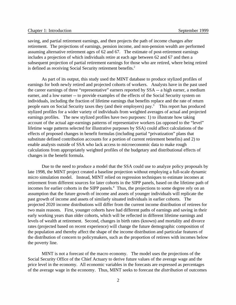
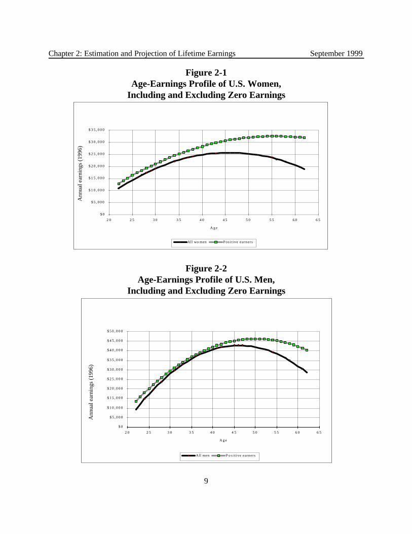
The profile of annual earned income over the lifetime has a characteristic hump-shapedpattern for typical Americans. Initial earnings are low, reflecting workers’ initially modest levelsof job tenure, skill, and experience. Earnings rise over time, often in an erratic pattern, as workersaccumulate human capital and find jobs that offer wages reflecting the workers’ greater skill andjob experience. Earnings then fall, either abruptly, as a result of worker retirement or disability,or more gradually, as a result of declining work hours, employer discrimination, or the erodingvalue of a worker’s skills
The characteristic pattern of lifetime earnings profiles is displayed in Figures 2-1 and 2-2,which show the cross-sectional pattern of earned income among women and men, respectively. The higher line in each figure shows the age profile of earnings among all workers who hadpositive earned incomes in 1996. The profile is estimated as a quadratic function of age usingCensus Bureau tabulations of average earnings within broad age categories (age 18-24, 25-34,35-44, and so on). For both women and men the age pattern of earned income, conditional onhaving positive earnings, shows a rapid rise from ages 22 through 40, slower earnings growth forworkers in their 40s, and earnings declines beginning sometime after age 50.
The lower and heavier line in the two figures shows the lifetime profile of average earningscalculated using information from all potential workers, including those who do not work. Thisline shows lower average earnings at each age, especially among women, but it reveals the samecharacteristic pattern of rapidly rising income when workers are in their 20s and 30s and decliningearnings when they are in their 50s and 60s. The estimated peak of expected earnings occurs atan earlier age when people with zero earnings are included in the tabulations. This is because theunconditional earnings profile also incorporates the effects of labor force withdrawal of workerswho become disabled or who retire. Since disability and early retirement become more commonas workers reach their 50s, the fall in unconditional earnings begins at a younger age.
The lines in the two figures clearly do not represent the earnings experiences of each U.S.worker. Instead they reflect the experiences in a single year of all workers when their experiencesare averaged together. The cross-sectional pattern of earnings differs widely for workers withdifferent characteristics. The figures show that the patterns for women and men differ noticeably,for example. In comparison with workers who have limited education, workers
Chapter 2: Estimation and Projection of Lifetime Earnings September 1999
9
$ 0
$ 5 , 0 0 0
$ 1 0 , 0 0 0
$ 1 5 , 0 0 0
$ 2 0 , 0 0 0
$ 2 5 , 0 0 0
$ 3 0 , 0 0 0
$ 3 5 , 0 0 0
2 0 2 5 3 0 3 5 4 0 4 5 5 0 5 5 6 0 6 5
A g e
Ann
ual e
arni
ngs
(199
6)
All wo men Posi t ive earners
$ 0
$ 5 , 0 0 0
$ 1 0 , 0 0 0
$ 1 5 , 0 0 0
$ 2 0 , 0 0 0
$ 2 5 , 0 0 0
$ 3 0 , 0 0 0
$ 3 5 , 0 0 0
$ 4 0 , 0 0 0
$ 4 5 , 0 0 0
$ 5 0 , 0 0 0
2 0 2 5 3 0 3 5 4 0 4 5 5 0 5 5 6 0 6 5
A g e
Ann
ual e
arni
ngs
(199
6)
All men P o s itive earners
Figure 2-1Age-Earnings Profile of U.S. Women,
Including and Excluding Zero Earnings
Figure 2-2Age-Earnings Profile of U.S. Men,
Including and Excluding Zero Earnings

Chapter 2: Estimation and Projection of Lifetime Earnings September 1999
10
with more schooling show a characteristic pattern of steeper earnings growth in their 20s and 30s,and their earnings typically reach a lifetime peak at a later age. The age profile of earnings has notremained fixed over the past few decades. In the 1960s, the cross-sectional age pattern ofearnings showed smaller earnings differences between 25-year-old and 45-year-old workers. Inother words, the age profile of earnings is now more steeply sloped than it was in the past. Finally, individual workers differ widely from one another. Even among workers with identicalobservable characteristics, including age, educational attainment, occupational attachment, andjob tenure, there are enormous variations in annual earnings and in the pattern of year-to-yearearnings change.
1. Basic Specification
To make a forecast of future earnings for workers who have only partially completed theircareers, it is necessary to make credible predictions about the structure of future age-earningsprofiles. We adopted a simple specification of the basic relation between workers’ ages and thechange in their earnings. Individual-level earnings is treated as a step-function of age. Inparticular,
yit = µ i + f(Age) + ,it, (1)where
f(Age) = $1 A1 + $2 A2 + $3 A3 + ... + $T AT , and A1 = 1 if Age is less than 25,
= 0, otherwise; A2 = 1 if Age is between 25 and 29,
= 0, otherwise; A3 = 1 if Age is between 30 and 34,
= 0, otherwise; A4 = 1 if Age is between 35 and 39,
= 0, otherwise; [This category is omitted in the estimation.] A5 = 1 if Age is between 40 and 44,
= 0, otherwise; A6 = 1 if Age is between 45 and 49,
= 0, otherwise; A7 = 1 if Age is between 50 and 54,
= 0, otherwise; A8 = 1 if Age is between 55 and 57,
= 0, otherwise; A9 = 1 if Age is between 58 and 59,
= 0, otherwise; A10 = 1 if Age is between 60 and 61,
= 0, otherwise; A11 = 1 if Age is 62,
= 0, otherwise; A12 = 1 if Age is between 63 and 64,

Chapter 2: Estimation and Projection of Lifetime Earnings September 1999
11
= 0, otherwise; A13 = 1 if Age is 65,
= 0, otherwise; A14 = 1 if Age is 66 or more,
= 0, otherwise.
Ignoring µ i and ,it , this specification implies that earnings rise by varying amounts, $A , at eachof the age breaks specified in the function f(Age). This specification is obviously far more flexiblethan the quadratic function used to estimate the cross-sectional age-earnings profiles in Figures 2-1 and 2-2.
Economists have scant basis for predicting the future trend of economy-wide averageearnings. This trend will obviously have a crucial influence on the earnings profile of workerswho are currently young or middle-aged. Rather than estimate the trend in economy-wideearnings directly, we estimate the relationship between workers’ relative earnings and their age. Relative earnings in this study is defined as the ratio of a worker’s earnings in a given year to theeconomy-wide average covered wage estimated by the Social Security Administration. Thus, thecoefficients $A in equation (1) refer to the change in a worker’s relative earnings at each of theage breaks in the age-earnings function, f(Age). If economy-wide average earnings climb rapidly,the $’s will be associated with steep growth in actual earnings during the phase in a worker’scareer when his or her relative earnings are climbing. If economy-wide real wages are stagnant ordeclining, the $’s will be associated with very modest or even shrinking annual earnings.
As noted above, the pattern of career earnings differs across population groups. Earningsprofiles differ between men and women and among workers with differing levels of educationalattainment. In this study, we estimated separate earnings functions for men and women, who inturn are divided into five educational groups: those who did not complete high school; those witha high school diploma but no schooling beyond high school; those with one to three years ofcollege education; those with a college diploma; and those with at least one year of educationbeyond college. Workers can of course be divided into even narrower categories, for example, byrace, occupational attachment, marital status, and geographic region. In order to keep theestimation and projection simple, we decided not to examine career earnings profiles in thesenarrower groups. Several of them, including occupation and marital status, can change over aworker’s career. Since we observe these time-varying variables only up through the time anindividual is last interviewed, we cannot reliably predict how these variables will change over theremainder of the worker’s career. For this reason, we do not think it makes sense to include themat this stage in the estimation model.
We estimated the earnings equation under a fixed-effect specification. That is, we assumethat each person in a given sub-population differs from other workers in his or her peer group bya fixed average amount. This individual-specific difference persists over a worker’s entire careerand is captured by the error term µ i in equation 1 above. Under the assumptions of the fixed-
Chapter 2: Estimation and Projection of Lifetime Earnings September 1999
12
effect model, we cannot obtain estimates of coefficients of variables that do not change over timefor a single observation. The effects of these variables are all captured by the person-specificindividual effect. Thus, we do not obtain coefficient estimates in the earnings regressions of theeffects of a person’s race or birth cohort, because these variables do not change over time forpeople in the sample. (If analysts want to know the average effects of these variables, they cancalculate the average value of the estimated fixed effects of respondents with the relevantcharacteristics.)
The coefficients of the age terms, $A ,are essentially determined by the average observedchange in relative earnings as workers move up from one age category to the next. For example,the coefficient $3 shows the average difference in earnings between ages 30-34 and the omittedage category, ages 35-39. This is determined by an estimate of the average gain in relativeearnings that persons actually experienced between ages 30-34, on the one hand, and ages 35-39,on the other. This kind of estimate can only be obtained with longitudinal information for asample of workers. (It is not an estimate of the average difference in earnings between peoplewho are 30-34 and people who are 35-39 in a given year.)
For estimates based on this model to be valid, it must be the case that future relativeearnings increases will mirror the pattern observed during the period covered by the estimationsample. Suppose the sample consists of people born between 1931 and 1960, and earnings areobserved for the period from 1981 to 1990. The oldest people in the sample are between 50 and60 years old during the estimation period. From the experiences of these people we can formestimates of the average increase or decline in earnings that takes place between ages 50-54, 55-57, and 58-59. Under the assumptions of the model, the relative earnings gains or lossesexperienced by this cohort will be duplicated by later cohorts when they reach ages 50-54, 55-57,and 58-59. Of course, the actual average earnings of younger cohorts will differ from those of theolder cohort. The model offers two possible explanations for the difference. First, if economy-wide earnings grow faster when the younger cohorts are between 50 and 60, their actual earningswill grow faster (or decline more slowly) than was the case for the older cohort. Second, theaverage value of the individual specific error term, µ i , may differ between the two cohorts,although the difference between two large birth cohorts will probably be small.
2. Employment Patterns
The specification defined by equation 1 represents a single-equation model of the earningsgeneration process. We emphasize that this approach does not adequately account for thephenomenon of worker retirement. It would be desirable to expand the model to produceseparate estimates of the career pattern of employment and the career path of earnings,conditional on employment. Some workers leave the labor force at a comparatively young age asa result of disability or early retirement. These workers may have rising earnings up through thepoint they leave the labor force. In a single-equation model of earnings, the effects of the labormarket withdrawal of these early retirees is combined with the effects of continued earnings gains

Chapter 2: Estimation and Projection of Lifetime Earnings September 1999
13
among workers who remain employed. The estimates of the $A will provide reasonable estimatesof the path of unconditional earnings, that is, earnings of workers and nonworkers alike. Unfortunately, they will obscure the potentially distinctive path of average earnings of thoseworkers who remain employed. Equally important, they fail to reflect the abrupt drop in earningsthat often accompanies worker retirement or disability.
Although we attempted to estimate a joint model that predicts employment status andaverage earnings conditional on employment, we encountered two problems implementing themodel for purposes of making predictions of future earnings. First, the estimates of theemployment equation did not produce very reliable predictions of employment. Unless we usedinformation about each person’s actual employment status in the past one or two years, we didnot reliably predict the person’s employment status in subsequent periods. While it might seemlogical to modify the basic employment specification to include additional information about eachperson’s actual employment status in past periods, we do not think this modification would beappropriate without thorough specification tests. Unless we can be confident that we know thecorrect specification of the effect of past employment status on current status, it is dangerous tomake long-range predictions of future employment status based on a specification that includeslagged employment status. (This is true whether the specification explicitly includes pastemployment status as a regressor or it includes an auto-regressive specification of the disturbanceterm.) Including such lagged employment information in the specification is helpful in producingreasonably accurate -- though possibly biased -- predictions of employment status in the nextperiod, or even in the next three or four periods. But small misspecification errors can generatelarge and systematic prediction errors in longer term forecasts. (In this project, we makepredictions 25 or more years into the future for some of the youngest sample members.) Tominimize the possibility of large out-of-sample prediction errors, analysts should closelyinvestigate the proper time-series specification of the employment equation. Given the time andresource limits of this project, we did not think this was feasible.
A second forecasting problem associated with the two-equation approach to estimationarises because of the logical relationship between the employment-prediction and earnings-prediction equations. The estimated employment-prediction equation explains less than 100percent of the actual variation in employment status. From the estimated employment equationwe can generate predictions of future employment status over the next one to twenty-five years byusing a sequence of random numbers to determine whether an individual has covered earnings insuccessive future years. This prediction method often produces the prediction that a person whohas a very low probability of employment -- and very low or negative expected earnings -- willnonetheless be employed. The problem of producing a reasonable prediction of earnings for suchan individual is formidable unless the employment-prediction and earnings-prediction equationshave been simultaneously estimated, an undertaking that is well beyond the scope of this project.
Chapter 2: Estimation and Projection of Lifetime Earnings September 1999
14
3. Estimation Procedures
The earnings equation is estimated with data from the 1990-1993 Survey of Income and ProgramParticipation (SIPP) panels matched to Social Security Summary Earnings Records (SER). Thesample consisted of 44,792 women and 40,794 men for whom matched SIPP and SER recordscould be obtained. The sample was restricted to SIPP respondents in the 1990-1993 waves whocompleted the second periodic interview. (By implication the sample of “full responders” to theSIPP interviews – persons who completed all interviews that were offered to them – represents asubsample of the respondents to the second periodic interview.) The sample was furtherrestricted to persons born between 1926 and 1965.1
The SER records contain information on Social-Security-covered earnings by calendaryear for the period from 1951 through 1996. These records do not contain information about alllabor earnings, but only on earnings up to the taxable wage ceiling. Censoring at the taxablemaximum wage is a major problem for men in the sample, though not for women. According toour tabulations of the estimation sample, less than 1 percent of the person-year observations ofwomen in the sample are affected by censoring. (For example, women attained the taxablemaximum earnings less than 1 percent of the time between 1974 and 1983.) The problem is muchmore serious for men in the sample. Men’s Social Security covered earnings were affected bycensoring in about 15 percent of person years between 1974 and 1983. Among men bornbetween 1921 and 1960 who were at least 22 years old, 23 percent earned wages above thetaxable maximum at least once between 1984 and 1993 (when the taxable maximum was higher)and 13 percent earned wages above the taxable maximum at least once between 1994 and 1996. Men with above-average expected earnings -- for example, college graduates between 35 and 55years old -- face a high likelihood of reaching the taxable maximum in a given year.
Censoring would not be a concern if the taxable maximum remained relatively constant. Unfortunately, it increased over the analysis period, possibly giving rise to an upward bias inestimates of the growth rate in earnings for men who have high expected earned incomes. Although we did not implement a formal censoring model, we thought it would be useful to takeaccount of the censoring problem in a less formal and less costly way (though only in the case ofmales). As part of the work on stylized earnings profiles reported in Chapter 8, we createdestimates of “expected earnings above the taxable maximum, but below 2.46 times averageeconomy-wide earnings” for all men with Social Security covered earnings at the taxablemaximum. For brevity, we shall refer to this transformed measure of earnings as “less censored”earnings. (This measure of earnings is also used in Chapter 8 of the project, where it wasoriginally developed for analysis of stylized lifetime earnings patterns.)
In adjusting the censored earnings data, we did not alter the wage data for years after1989, nor did we alter any wage reports when the reported wage was below the taxable ceiling. Starting in 1990, the Social Security taxable maximum reached 2.46 times average earnings,where it has remained. We adjusted the pre-1990 wage reports to reflect a hypothetical wage

Chapter 2: Estimation and Projection of Lifetime Earnings September 1999
15
ceiling equivalent to the average wage ceiling of the 1990-96 period -- that is, a ceiling equal to2.46 times average earnings.
For earnings in the 1951-77 period, the SER contains information on the quarter in whichan individual’s wages reached the taxable ceiling. This information is used to impute annualearnings for men at the taxable wage ceiling under the following rules:
Quarter reached Range of potential earnings Predicted maximum (multiples of taxable maximum) mean of class
4 1 < w < 4/3 1.143 4/3 < w < 2 1.532 2 < w < 4 2.361 4 < w 5.00
The first column shows the calendar quarter in which an individual is known to haveattained the taxable wage ceiling. The second shows the probable earnings range of the individualunder the assumption that he earns steady wages throughout the year. For example, a workerwho attains the taxable maximum in the fourth quarter might have attained the maximum on thelast day of the quarter (in which case he earned exactly the ceiling wage) or on the first day of thequarter (in which case he earned 4/3 times the ceiling wage). Given this estimate of the potentialearnings range of each worker, we then derived an estimate of his expected earnings if hisearnings were in the predicted range. The class means were derived from the observeddistribution of wages in the Current Population Surveys (CPS) of 1965, 1970, 1975. Theestimated class means were very similar for all three survey years. These average values wereused to impute wages to workers above the taxable maximum for all of the years between 1951and 1977. The resulting wage values were truncated at a value of 2.46 times the economy-wideaverage wage to make them consistent in their expected value with the reported data for 1990-96.
For the period 1978-89, the CPS of each year was used to obtain information on thedistribution of wages in excess of that year’s taxable maximum. Those wage distributions weretruncated at 2.46 times the average wage, and the resulting expected values used to compute anaverage wage in excess of each year’s taxable maximum but below 2.46 times average earnings. That conditional average wage was used in place of the value of the ceiling wage.
Once we obtained these estimates of earnings for men at the taxable wage ceiling, we stillhad to decide how they should be used in estimation and prediction. We chose to include “lesscensored earnings” as the dependent variable in an earnings regression otherwise specified in thesame way as our standard earnings regression. We then compared the predictive power of theresulting estimates with those of the standard regression equation (i.e, the equation estimated onSocial Security covered earnings censored at the taxable wage ceiling). The average absoluteprediction error is somewhat smaller using results obtained using “less censored earnings.”2

Chapter 2: Estimation and Projection of Lifetime Earnings September 1999
16
III. ESTIMATES AND EARNINGS FORECASTS
The dependent variable in the estimation is the worker’s annual Social-Security-coveredearnings divided by the economy-wide average wage for the relevant year. This ratio, which isdesignated yi in equation 1, is multiplied by 100 to convert it into percentage terms. For men inthe sample, “less censored earnings” is substituted for Social-Security-covered earnings incalculating the earnings ratio.
The period used in estimation is 1987 through 1996, the last ten years of availableearnings data on the SER. Since the SER records cover wages earned back through 1951, weexperimented with longer estimation periods. However, we have little confidence in thepredictions generated using a substantially longer estimation period. Between 1973 and thepresent, American workers have experienced dramatic changes in lifetime earnings patterns. Thegap between low-, middle-, and high-wage workers increased significantly after 1979. Paydifferentials between women and men narrowed sharply. Wages of young workers fell noticeablyin comparison with wages paid to middle-aged and older workers. These trends have slowed orleveled off since the late 1980s. When the estimation period includes the ten years from 1977-1986 as well as later years, the estimated coefficients imply that many of the trends observed inthe late 1970s and early 1980s will continue into the indefinite future. We do not think thisprediction is plausible. For that reason, we restricted the estimation period to the years since1986, when many earnings patterns have stabilized. For each birth cohort included in the sample,the 10-year estimation period allows each cohort to move between at least two and possibly asmany as six age categories defined in the age-earnings function, f(Age).
1. Coefficient Estimates
The basic earnings equation was separately estimated in eight different samples, defined bygender and educational attainment. Respondents in the highest two educational attainmentgroups were combined into a single estimation sample; the other three educational groups wereincluded in separate estimation samples. The coefficient estimates, their standard errors, and 95-percent confidence intervals are displayed in Tables 2-1 and 2-2, which contain results for womenand men, respectively.
Since separate age-earnings profiles are estimated for college graduates and people withpost-college education, we estimate a total of 10 earnings profiles, five for women and five formen. The average estimated age-earnings profiles are displayed in Figure 2-3. The top panelshows the age-earnings profiles for five educational classes of women; the lower panel shows theprofiles for men. Note that men and women with greater educational attainment have significantlyhigher earnings than lower education groups at all ages past about age 30. Their peak careerearnings are also achieved somewhat later in life.3 These estimates imply that relative earningsbegin to decline for men between ages 40 and 50. Among men with the least

Chapter 2: Estimation and Projection of Lifetime Earnings September 1999
17
Table 2-1Female Age-Earnings Profiles, by Educational Attainment
Fixed-Effect Model Estimates
Education = Less than four years of high school. Fixed-effects (within) regressionsd(u_id) = 31.40634 Number of obs = 74357sd(e_id_t) = 17.63622 n = 7687sd(e_id_t + u_id) = 36.01936 T-bar = 9.67308corr(u_id, Xb) = 0.0115 R-sq within = 0.0295 between = 0.0309 overall = 0.0277 F( 13, 66657) = 155.80 Prob > F = 0.0000------------------------------------------------------------------------------ yratio | Coef. Std. Err. t P>|t| [95% Conf. Interval]---------+-------------------------------------------------------------------- Age24 | -12.29271 .7160332 -17.168 0.000 -13.69613 -10.88928 Age29 | -7.413093 .4267999 -17.369 0.000 -8.24962 -6.576565 Age34 | -3.989375 .3190682 -12.503 0.000 -4.614749 -3.364002 Age44 | 1.516319 .3318492 4.569 0.000 .8658951 2.166744 Age49 | 1.498146 .4367033 3.431 0.001 .6422076 2.354084 Age54 | -.8577039 .526687 -1.628 0.103 -1.89001 .1746024 Age57 | -3.946682 .608706 -6.484 0.000 -5.139746 -2.753619 Age59 | -6.165832 .6629575 -9.300 0.000 -7.465228 -4.866435 Age61 | -8.670656 .6858993 -12.641 0.000 -10.01502 -7.326294 Age62 | -11.72871 .7600354 -15.432 0.000 -13.21837 -10.23904 Age64 | -16.46597 .7275347 -22.633 0.000 -17.89194 -15.04 Age65 | -19.38252 .8203293 -23.628 0.000 -20.99036 -17.77467 Age67 | -21.67292 .8536696 -25.388 0.000 -23.34611 -19.99973 _cons | 27.08451 .323921 83.615 0.000 26.44963 27.7194------------------------------------------------------------------------------ id | F(7686,66657) = 31.175
Education = Four years of high school.sd(u_id) = 43.81776 Number of obs = 174680sd(e_id_t) = 22.76773 n = 17769sd(e_id_t + u_id) = 49.37981 T-bar = 9.8306corr(u_id, Xb) = 0.0397 R-sq within = 0.0279 between = 0.0353 overall = 0.0292 F( 13,156898) = 346.19 Prob > F = 0.0000------------------------------------------------------------------------------ yratio | Coef. Std. Err. t P>|t| [95% Conf. Interval]---------+-------------------------------------------------------------------- Age24 | -10.89394 .5343841 -20.386 0.000 -11.94132 -9.846557 Age29 | -7.162824 .3191782 -22.441 0.000 -7.788407 -6.537241 Age34 | -4.314175 .2373817 -18.174 0.000 -4.779438 -3.848912 Age44 | 3.997877 .2495359 16.021 0.000 3.508791 4.486962 Age49 | 5.875282 .3386881 17.347 0.000 5.211461 6.539104 Age54 | 4.455451 .424028 10.507 0.000 3.624365 5.286537 Age57 | 1.000265 .5142488 1.945 0.052 -.0076523 2.008181 Age59 | -2.859324 .5814337 -4.918 0.000 -3.998922 -1.719726 Age61 | -6.803079 .615085 -11.060 0.000 -8.008633 -5.597525 Age62 | -12.33316 .7109171 -17.348 0.000 -13.72654 -10.93978 Age64 | -20.02395 .6727037 -29.766 0.000 -21.34243 -18.70546 Age65 | -24.95934 .8005149 -31.179 0.000 -26.52834 -23.39035 Age67 | -27.52117 .8508359 -32.346 0.000 -29.1888 -25.85355 _cons | 46.38095 .2162292 214.499 0.000 45.95714 46.80475------------------------------------------------------------------------------ id | F(17768,156898) = 36.405

Chapter 2: Estimation and Projection of Lifetime Earnings September 1999
18
Table 2-1 (continued)
Education = One to three years of college.sd(u_id) = 52.99556 Number of obs = 95846sd(e_id_t) = 28.36678 n = 9687sd(e_id_t + u_id) = 60.10993 T-bar = 9.89429corr(u_id, Xb) = -0.0288 R-sq within = 0.0211 between = 0.0113 overall = 0.0114 F( 13, 86146) = 143.02 Prob > F = 0.0000------------------------------------------------------------------------------ yratio | Coef. Std. Err. t P>|t| [95% Conf. Interval]---------+-------------------------------------------------------------------- Age24 | -16.69987 .8274249 -20.183 0.000 -18.32162 -15.07813 Age29 | -8.444023 .4972576 -16.981 0.000 -9.418643 -7.469402 Age34 | -4.359475 .3686321 -11.826 0.000 -5.081991 -3.636959 Age44 | 7.01602 .3840808 18.267 0.000 6.263225 7.768815 Age49 | 10.95157 .5347588 20.479 0.000 9.903446 11.99969 Age54 | 11.76471 .7147145 16.461 0.000 10.36387 13.16554 Age57 | 9.532564 .9227685 10.330 0.000 7.723946 11.34118 Age59 | 4.897057 1.08578 4.510 0.000 2.768937 7.025177 Age61 | -.1251351 1.16581 -0.107 0.915 -2.410112 2.159842 Age62 | -6.855312 1.392399 -4.923 0.000 -9.584402 -4.126221 Age64 | -12.16573 1.306853 -9.309 0.000 -14.72715 -9.604307 Age65 | -18.95678 1.614956 -11.738 0.000 -22.12208 -15.79148 Age67 | -23.27936 1.722018 -13.519 0.000 -26.6545 -19.90422 _cons | 59.27902 .3021222 196.209 0.000 58.68687 59.87118------------------------------------------------------------------------------ id | F(9686,86146) = 33.950
Education = Four or more years of college.sd(u_id) = 71.29666 Number of obs = 95633sd(e_id_t) = 36.67594 n = 9649sd(e_id_t + u_id) = 80.17691 T-bar = 9.91118corr(u_id, Xb) = -0.0931 R-sq within = 0.0412 between = 0.0018 overall = 0.0058 F( 26, 85958) = 141.94 Prob > F = 0.0000------------------------------------------------------------------------------ yratio | Coef. Std. Err. t P>|t| [95% Conf. Interval]---------+-------------------------------------------------------------------- Age24 | -36.01407 1.235241 -29.156 0.000 -38.43513 -33.59301 Age29 | -6.185295 .7504073 -8.243 0.000 -7.656087 -4.714503 Age34 | -3.943033 .5617955 -7.019 0.000 -5.044147 -2.841919 Age44 | 6.572365 .5919927 11.102 0.000 5.412064 7.732666 Age49 | 13.72039 .8280236 16.570 0.000 12.09747 15.3433 Age54 | 16.02367 1.136902 14.094 0.000 13.79535 18.25199 Age57 | 14.26148 1.495558 9.536 0.000 11.3302 17.19276 Age59 | 9.550628 1.769274 5.398 0.000 6.082866 13.01839 Age61 | 2.559956 1.899944 1.347 0.178 -1.163918 6.28383 Age62 | -5.300336 2.323021 -2.282 0.023 -9.853437 -.7472344 Age64 | -15.21764 2.173822 -7.000 0.000 -19.47832 -10.95697 Age65 | -23.69783 2.70219 -8.770 0.000 -28.9941 -18.40156 Age67 | -32.56209 2.897974 -11.236 0.000 -38.24209 -26.88208Ag24_Ed5 | -38.57714 2.69157 -14.333 0.000 -43.85259 -33.30169Ag29_Ed5 | -21.28159 1.529356 -13.915 0.000 -24.27911 -18.28406Ag34_Ed5 | -5.72276 1.086691 -5.266 0.000 -7.852666 -3.592854Ag44_Ed5 | 2.601815 1.018081 2.556 0.011 .6063849 4.597244Ag49_Ed5 | 2.579371 1.39273 1.852 0.064 -.1503689 5.30911Ag54_Ed5 | 5.545336 1.871429 2.963 0.003 1.877352 9.21332Ag57_Ed5 | 3.822669 2.504238 1.526 0.127 -1.085616 8.730954Ag59_Ed5 | -3.725834 2.981212 -1.250 0.211 -9.568984 2.117316Ag61_Ed5 | -4.334154 3.249751 -1.334 0.182 -10.70364 2.03533Ag62_Ed5 | -5.003977 3.939414 -1.270 0.204 -12.7252 2.717242Ag64_Ed5 | -12.50108 3.70212 -3.377 0.001 -19.75721 -5.24496Ag65_Ed5 | -14.97261 4.604314 -3.252 0.001 -23.99703 -5.948195Ag67_Ed5 | -10.07044 4.890624 -2.059 0.039 -19.65602 -.4848578 _cons | 82.99281 .3778786 219.628 0.000 82.25217 83.73345------------------------------------------------------------------------------ id | F(9648,85958) = 36.224

Chapter 2: Estimation and Projection of Lifetime Earnings September 1999
19
Table 2-2Male Age-Earnings Profiles, by Educational Attainment
Fixed-Effect Model Estimates
Education = Less than four years of high school. Fixed-effects (within) regressionsd(u_id) = 56.7756 Number of obs = 68975sd(e_id_t) = 31.80853 n = 7140sd(e_id_t + u_id) = 65.07881 T-bar = 9.66036corr(u_id, Xb) = -0.2280 R-sq within = 0.1053 between = 0.0235 overall = 0.0304 F( 13, 61822) = 559.40 Prob > F = 0.0000------------------------------------------------------------------------------ yratio | Coef. Std. Err. t P>|t| [95% Conf. Interval]---------+-------------------------------------------------------------------- Age24 | -18.09379 1.254757 -14.420 0.000 -20.55312 -15.63446 Age29 | -7.052151 .7727004 -9.127 0.000 -8.566645 -5.537656 Age34 | -2.235293 .5886969 -3.797 0.000 -3.38914 -1.081446 Age44 | -.7398771 .6387606 -1.158 0.247 -1.991849 .5120951 Age49 | -5.870017 .8451327 -6.946 0.000 -7.526479 -4.213555 Age54 | -13.09429 1.012529 -12.932 0.000 -15.07885 -11.10973 Age57 | -26.52734 1.164159 -22.787 0.000 -28.80909 -24.24558 Age59 | -34.78413 1.263135 -27.538 0.000 -37.25988 -32.30838 Age61 | -44.95629 1.305595 -34.434 0.000 -47.51526 -42.39732 Age62 | -56.97512 1.443249 -39.477 0.000 -59.80389 -54.14635 Age64 | -76.24629 1.382756 -55.141 0.000 -78.95649 -73.53608 Age65 | -88.4447 1.571482 -56.281 0.000 -91.52481 -85.36459 Age67 | -95.51312 1.626268 -58.731 0.000 -98.70061 -92.32563 _cons | 78.85383 .6119618 128.854 0.000 77.65439 80.05328------------------------------------------------------------------------------ id | F(7139,61822) = 28.748
Education = Four years of high school.sd(u_id) = 64.88506 Number of obs = 140285sd(e_id_t) = 35.38793 n = 14230sd(e_id_t + u_id) = 73.9079 T-bar = 9.8584corr(u_id, Xb) = -0.1640 R-sq within = 0.0756 between = 0.0291 overall = 0.0308 F( 13,126042) = 792.46 Prob > F = 0.0000------------------------------------------------------------------------------ yratio | Coef. Std. Err. t P>|t| [95% Conf. Interval]---------+-------------------------------------------------------------------- Age24 | -19.81902 .8722068 -22.723 0.000 -21.52853 -18.10951 Age29 | -7.842719 .5171317 -15.166 0.000 -8.856288 -6.82915 Age34 | -.9857611 .3810928 -2.587 0.010 -1.732696 -.2388258 Age44 | -1.930576 .4260428 -4.531 0.000 -2.765613 -1.09554 Age49 | -7.554708 .60333 -12.522 0.000 -8.737225 -6.372192 Age54 | -17.07835 .7593425 -22.491 0.000 -18.56665 -15.59005 Age57 | -30.66509 .9234691 -33.206 0.000 -32.47507 -28.85511 Age59 | -44.29774 1.055965 -41.950 0.000 -46.36741 -42.22806 Age61 | -59.72219 1.122345 -53.212 0.000 -61.92197 -57.52242 Age62 | -75.31036 1.314187 -57.306 0.000 -77.88614 -72.73457 Age64 | -94.51296 1.242308 -76.079 0.000 -96.94786 -92.07805 Age65 | -109.1274 1.49186 -73.149 0.000 -112.0514 -106.2034 Age67 | -117.2749 1.579743 -74.237 0.000 -120.3712 -114.1786 _cons | 107.1683 .3496285 306.521 0.000 106.4831 107.8536------------------------------------------------------------------------------ id | F(14229,126042) = 31.504

Chapter 2: Estimation and Projection of Lifetime Earnings September 1999
20
Table 2-2 (continued)
Males: Education = One to three years of college.sd(u_id) = 71.31912 Number of obs = 82523sd(e_id_t) = 39.21926 n = 8332sd(e_id_t + u_id) = 81.39145 T-bar = 9.90434corr(u_id, Xb) = -0.1384 R-sq within = 0.0677 between = 0.0220 overall = 0.0263 F( 13, 74178) = 414.62 Prob > F = 0.0000------------------------------------------------------------------------------ yratio | Coef. Std. Err. t P>|t| [95% Conf. Interval]---------+-------------------------------------------------------------------- Age24 | -35.40504 1.269636 -27.886 0.000 -37.89352 -32.91656 Age29 | -14.86891 .7660261 -19.410 0.000 -16.37032 -13.3675 Age34 | -3.431996 .5596867 -6.132 0.000 -4.52898 -2.335012 Age44 | -1.634919 .5545853 -2.948 0.003 -2.721904 -.5479341 Age49 | -7.925679 .7744412 -10.234 0.000 -9.44358 -6.407777 Age54 | -17.46588 1.043255 -16.742 0.000 -19.51066 -15.42111 Age57 | -34.90784 1.353062 -25.799 0.000 -37.55984 -32.25584 Age59 | -48.89085 1.583633 -30.873 0.000 -51.99476 -45.78693 Age61 | -65.27757 1.696596 -38.476 0.000 -68.60289 -61.95225 Age62 | -82.87883 2.035584 -40.715 0.000 -86.86856 -78.88909 Age64 | -102.2858 1.909873 -53.556 0.000 -106.0291 -98.54241 Age65 | -120.5922 2.404062 -50.162 0.000 -125.3042 -115.8803 Age67 | -131.7692 2.57832 -51.107 0.000 -136.8227 -126.7157 _cons | 121.7559 .4490658 271.132 0.000 120.8758 122.6361------------------------------------------------------------------------------ id | F(8331,74178) = 31.343
Males: Education = Four or more years of college.sd(u_id) = 80.13025 Number of obs = 109631sd(e_id_t) = 44.22211 n = 11092sd(e_id_t + u_id) = 91.52296 T-bar = 9.88379corr(u_id, Xb) = -0.0321 R-sq within = 0.1027 between = 0.0505 overall = 0.0594 F( 26, 98513) = 433.51 Prob > F = 0.0000------------------------------------------------------------------------------ yratio | Coef. Std. Err. t P>|t| [95% Conf. Interval]---------+-------------------------------------------------------------------- Age24 | -82.24171 1.525664 -53.906 0.000 -85.23199 -79.25143 Age29 | -33.71748 .9484911 -35.549 0.000 -35.57651 -31.85844 Age34 | -7.874092 .7164915 -10.990 0.000 -9.278407 -6.469777 Age44 | 2.157216 .7038325 3.065 0.002 .7777123 3.536719 Age49 | -.0161685 .9500128 -0.017 0.986 -1.878182 1.845845 Age54 | -8.21484 1.280029 -6.418 0.000 -10.72368 -5.705999 Age57 | -24.02843 1.673674 -14.357 0.000 -27.30881 -20.74805 Age59 | -40.89005 1.952824 -20.939 0.000 -44.71756 -37.06254 Age61 | -57.72099 2.093298 -27.574 0.000 -61.82383 -53.61815 Age62 | -74.04065 2.519158 -29.391 0.000 -78.97817 -69.10313 Age64 | -94.50082 2.361653 -40.015 0.000 -99.12963 -89.87201 Age65 | -113.0157 2.929603 -38.577 0.000 -118.7577 -107.2737 Age67 | -127.6937 3.144102 -40.614 0.000 -133.8561 -121.5313Ag24_Ed5 | -44.49208 3.286473 -13.538 0.000 -50.93353 -38.05063Ag29_Ed5 | -33.26033 1.767411 -18.819 0.000 -36.72443 -29.79623Ag34_Ed5 | -10.8658 1.247064 -8.713 0.000 -13.31003 -8.421567Ag44_Ed5 | 2.400491 1.154966 2.078 0.038 .1367715 4.66421Ag49_Ed5 | 5.193227 1.52304 3.410 0.001 2.208087 8.178367Ag54_Ed5 | 7.662023 1.97888 3.872 0.000 3.783441 11.5406Ag57_Ed5 | 13.7329 2.556489 5.372 0.000 8.722213 18.74359Ag59_Ed5 | 17.8258 2.980079 5.982 0.000 11.98488 23.66672Ag61_Ed5 | 19.80614 3.193394 6.202 0.000 13.54712 26.06515Ag62_Ed5 | 22.54329 3.834117 5.880 0.000 15.02846 30.05811Ag64_Ed5 | 23.14078 3.602377 6.424 0.000 16.08016 30.20139Ag65_Ed5 | 18.61051 4.451451 4.181 0.000 9.885717 27.3353Ag67_Ed5 | 19.18038 4.770205 4.021 0.000 9.830832 28.52992 _cons | 154.5912 .4682512 330.146 0.000 153.6735 155.509------------------------------------------------------------------------------ id | F(11091,98513) = 32.151

Chapter 2: Estimation and Projection of Lifetime Earnings September 1999
21
Women
0.00
0.20
0.40
0.60
0.80
1.00
1.20
20 30 40 50 60 70
Age
Ear
ning
s / E
cono
my-
wid
e E
arni
ngs
Dropouts
High School Grads.
Some College
College Graduate
Post College
Men
-0.20
0.00
0.20
0.40
0.60
0.80
1.00
1.20
1.40
1.60
1.80
20 30 40 50 60 70
Age
Ear
ning
s / E
cono
my-
wid
e E
arni
ngs
Dropouts
High School Grads.
Some College
College Graduate
Post College
Figure 2-3Estimated Age-Earnings Profiles
By Sex and Educational Attainment

Chapter 2: Estimation and Projection of Lifetime Earnings September 1999
22
schooling attainment, relative earnings begin to fall as early as age 40. Men who have completedcollege do not experience sizable relative earnings declines until their 50s. Earnings peak at alower level but at a later age among women. Peak lifetime earnings are only slightly higher thanthe economy-wide average wage for women with college and post-graduate educations. Incontrast, among men with similar educational levels, peak earnings are approximately 60 percenthigher than economy-wide earnings. Whereas men experience sizable or at least modest drops inaverage earnings by age 55, well-educated women do not attain their peak lifetime earnings untiltheir middle 50s. Bear in mind that the age-earnings profiles displayed in Figure 2-3 show thecombined effects of changing annual earnings among people who continue to work full time aswell as steep earnings reductions associated with disability and early retirement for workersaffected by these phenomena. If the estimates were based solely on earnings patterns among menand women who continue to work full time, we would see a later and higher peak in lifetimeearnings.
2. Adjustments for Disability Onset
RAND Corporation analysts associated with this project generated two kinds ofpredictions that affect our projections of future earnings. They produced both a prediction of theonset of a health problem that limits the kind or amount of work a person can do and a predictionof the calendar year of death. The latter prediction was used to zero out predicted Social Securitycovered earnings for all years after the predicted date of death. RAND’s prediction of a healthlimitation was used to help predict the onset of Social Security Disability Insurance (DI) receipt. In this section, we explain how our estimates of DI onset were obtained and how they are used tomodify our forecast of earnings for people predicted to receive DI pensions.
We used data in the Social Security Administration’s Master Beneficiary Record (MBR)to derive an estimate of the onset of DI payments for matched SIPP-SER sample members. These estimates range back to 1957 (when the DI program was established) up through 1998. Because the MBR data show an unexpected decline in the incidence of new DI awards beginningin 1995, the MBR file does not fully reflect new DI awards in the 1995-98 period. We thereforeused the data for the calendar years 1987 - 1994 as a basis for estimating a Probit equation thatpredicts DI onset.
The Probit coefficients are displayed in Table 2-3, titled “Probit Model of DisabilityInsurance Onset by Gender, 1987 - 1994.” The age category variables are the same as thosedescribed above. In addition, the independent variables include race or ethnicity indicatorvariables (“black” and “whhis” -- white Hispanic), an indicator variable (“disabl”) derived fromRAND’s prediction of the onset of a health problem that limits the kind or amount of work aperson can do (set equal to zero in years before RAND predicts a health limit and set equal to onein later years), educational attainment indicator variables (“Edc1” through “Edc5”) associatedwith five levels of schooling (less than four years of high school, one to three years of college,four years of college, and five or more years of college; the omitted category is four years of high

Chapter 2: Estimation and Projection of Lifetime Earnings September 1999
23
school), and indicator variables (“avernc1” through “avernc6” or “avernc8”) that reflect theperson’s average Social Security covered earnings in the 10-year period ending in the calendaryear before the year in the estimation.
We developed our specification of the effect of past indexed earnings after someexperimentation with alternative approaches. Our first approach was to attempt to measureprecisely the eligibility status (except for level of health impairment) of each person in the sample. According to the Social Security Act, a person’s eligibility is determined under a two-part testthat involves the person’s total credited quarters of covered earnings and the level of coveredearnings in the recent past. To be eligible for a DI pension, a person suffering serious healthimpairment must meet both these tests. We tried to apply the tests for each year in the estimationperiod based on earnings information in the SER. According to our calculations, there were ahandful of people who began to receive DI pensions even though they did not pass both tests. Itis of course possible that our program did not accurately reflect the two-part test for eligibility. Itis probable that the person’s eligibility was determined on the basis of earnings received in aperiod different from the one we assumed.
The failure of our program to distinguish accurately between eligible and ineligibleworkers led us to take a different approach to the specification of DI onset. Workers with no orvery low covered earnings in the recent past should be ineligible for DI benefits. However,eligible workers with moderately low earnings are often found to have the highest propensity toapply for benefits. There are two likely reasons for this. First, workers with low recent earningshave low potential earnings. Under the redistributive formula that determines DI pensions, theseworkers receive benefits that are very generous relative to their potential earnings. The high replacement rate makes it financially more attractive for low-potential-earnings workers to applyfor DI. Second, a disproportionately large percentage of low-wage jobs are in manualoccupations with physically demanding work requirements. Health impairments are more likely tomake it impossible or very unpleasant to continue to work in these jobs. A reasonablespecification of the effect of lagged past earnings is that lagged earnings will have a nonlineareffect on the probability of DI onset. Zero and very low past earnings levels should make DIonset very improbable, because the person is not likely to meet the two-part earningsrequirements. Somewhat higher past earnings levels should be associated with above-averageprobability of DI onset. Further increases in lagged earnings above some threshold level shouldbe associated with declining probability of DI onset.
Our final specification of DI onset reflects this reasoning. We divided 10-year-laggedaverage earnings into 6 to 8 categories. The first category represents a very low level of 10-year-average earnings (15 percent or less of economy-wide average earnings), while other categoriesreflect successively higher levels of 10-year-average earnings. For calendar years 1977 - 1996,actual earnings are used to derive our estimates of 10-year-average earnings; for calendar years1997-2024, our predicted Social Security covered earnings are used.

Chapter 2: Estimation and Projection of Lifetime Earnings September 1999
24
Table 2-3Probit Model of Disability Insurance Onset
by Gender, 1987 - 1994
Dependent variable is onset of Social Security Disability Insurance /Sample each year consists of persons who have not begun receiving
DI as of December 31 of the previous calendar year. Females: Probit model of DI onset.
(Sum of weights is 5.5827e+011)
Probit Estimates Number of obs = 339323 chi2(21) =2118.29 Prob > chi2 = 0.0000Log Likelihood = -5165.8543 Pseudo R2 = 0.2035
(standard errors adjusted for clustering on newid)------------------------------------------------------------------------------ | Robust DI | Coef. Std. Err. z P>|z| [95% Conf. Interval]---------+-------------------------------------------------------------------- black | .1654386 .0355755 4.650 0.000 .0957119 .2351653 whhis | -.0848271 .0561367 -1.511 0.131 -.1948531 .0251989 disabl | 1.074342 .030751 34.937 0.000 1.014071 1.134612 Age34 | .0606031 .0654301 0.926 0.354 -.0676374 .1888437 Age39 | .0499833 .0677031 0.738 0.460 -.0827124 .1826789 Age44 | .153239 .0658025 2.329 0.020 .0242684 .2822095 Age49 | .2056123 .0655228 3.138 0.002 .07719 .3340345 Age54 | .379617 .0637878 5.951 0.000 .2545952 .5046389 Age57 | .5084386 .0678361 7.495 0.000 .3754824 .6413948 Age59 | .517327 .0711581 7.270 0.000 .3778598 .6567943 Age61 | .4578733 .072932 6.278 0.000 .3149292 .6008174 Age67 | .1240795 .0825009 1.504 0.133 -.0376193 .2857784 Edc1 | .2479518 .0333937 7.425 0.000 .1825013 .3134023 Edc3 | -.0484136 .037074 -1.306 0.192 -.1210773 .0242502 Edc4 | -.1559035 .0530473 -2.939 0.003 -.2598744 -.0519327 Edc5 | -.2161441 .0749549 -2.884 0.004 -.363053 -.0692351 avernc1 | -.6339791 .0411518 -15.406 0.000 -.7146351 -.5533231 avernc2 | -.0300959 .0375582 -0.801 0.423 -.1037087 .0435169 avernc4 | .0144312 .0406474 0.355 0.723 -.0652362 .0940985 avernc5 | .0288912 .0517097 0.559 0.576 -.072458 .1302405 avernc6 | -.0621247 .062069 -1.001 0.317 -.1837777 .0595283 _cons | -3.179644 .0578709 -54.944 0.000 -3.293069 -3.066219------------------------------------------------------------------------------
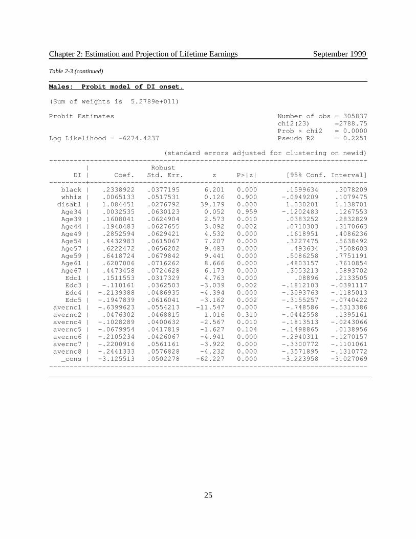
Chapter 2: Estimation and Projection of Lifetime Earnings September 1999
25
Table 2-3 (continued) Males: Probit model of DI onset.
(Sum of weights is 5.2789e+011)
Probit Estimates Number of obs = 305837 chi2(23) =2788.75 Prob > chi2 = 0.0000Log Likelihood = -6274.4237 Pseudo R2 = 0.2251
(standard errors adjusted for clustering on newid)------------------------------------------------------------------------------ | Robust DI | Coef. Std. Err. z P>|z| [95% Conf. Interval]---------+-------------------------------------------------------------------- black | .2338922 .0377195 6.201 0.000 .1599634 .3078209 whhis | .0065133 .0517531 0.126 0.900 -.0949209 .1079475 disabl | 1.084451 .0276792 39.179 0.000 1.030201 1.138701 Age34 | .0032535 .0630123 0.052 0.959 -.1202483 .1267553 Age39 | .1608041 .0624904 2.573 0.010 .0383252 .2832829 Age44 | .1940483 .0627655 3.092 0.002 .0710303 .3170663 Age49 | .2852594 .0629421 4.532 0.000 .1618951 .4086236 Age54 | .4432983 .0615067 7.207 0.000 .3227475 .5638492 Age57 | .6222472 .0656202 9.483 0.000 .493634 .7508603 Age59 | .6418724 .0679842 9.441 0.000 .5086258 .7751191 Age61 | .6207006 .0716262 8.666 0.000 .4803157 .7610854 Age67 | .4473458 .0724628 6.173 0.000 .3053213 .5893702 Edc1 | .1511553 .0317329 4.763 0.000 .08896 .2133505 Edc3 | -.110161 .0362503 -3.039 0.002 -.1812103 -.0391117 Edc4 | -.2139388 .0486935 -4.394 0.000 -.3093763 -.1185013 Edc5 | -.1947839 .0616041 -3.162 0.002 -.3155257 -.0740422 avernc1 | -.6399623 .0554213 -11.547 0.000 -.748586 -.5313386 avernc2 | .0476302 .0468815 1.016 0.310 -.0442558 .1395161 avernc4 | -.1028289 .0400632 -2.567 0.010 -.1813513 -.0243066 avernc5 | -.0679954 .0417819 -1.627 0.104 -.1498865 .0138956 avernc6 | -.2105234 .0426067 -4.941 0.000 -.2940311 -.1270157 avernc7 | -.2200916 .0561161 -3.922 0.000 -.3300772 -.1101061 avernc8 | -.2441333 .0576828 -4.232 0.000 -.3571895 -.1310772 _cons | -3.125513 .0502278 -62.227 0.000 -3.223958 -3.027069------------------------------------------------------------------------------

Chapter 2: Estimation and Projection of Lifetime Earnings September 1999
26
The exact definitions of the earnings categories, for women and men, respectively, are asfollows:
Range of 10-year-average earnings as % of economy-wide earnings Variable name Women Men
avernc1 0 - 15 percent 0 - 15 percent avernc2 15 - 30 15 - 30[ Left out category: 30 - 70 30 - 70 ] avernc4 70 - 100 70 - 100 avernc5 100 - 130 100 - 130 avernc6 130 percent or more 130 - 180 avernc7 ------ 180 - 210 avernc8 ------ 210 percent or more
The Probit equations were estimated using weights reflecting the SIPP 2nd interview panelweights. The weighted estimates are virtually identical to those obtained with unweightedestimation, but the predictions of future DI incidence using weighted estimation appeared slightlypreferable to those generated with coefficients obtained with unweighted estimation. (Inparticular, the rise in the predicted incidence of DI as the population ages after 1994 wassomewhat smoother using the weighted rather than unweighted coefficient estimates.)
We used information from the MBR to predict DI onset for those persons found to beginreceiving DI benefits between 1995 and 1997, inclusive. The people with records in the MBRthat show they began receiving DI between 1995-1997 were “predicted” to begin receivingbenefits in those years. The probability that other persons in the sample would experience DIonset was adjusted (i.e., was reduced) to reflect the existence of those persons already“predicted” to begin receiving DI because the MBR showed that they actually began to receive DIbetween 1995-1997. In years starting in 1998, persons were predicted to begin receiving a DIpension based solely on the probabilities predicted by the coefficient estimates in Table 2-3. Assignment to DI status was generated by comparing the person’s predicted probability of DIonset to a randomly selected number in the unit interval. Persons with a random number belowthe probability threshold implied by the Probit prediction were identified as beginning to receiveDI; persons with a random number above the threshold were identified as non-DI recipients forthe year. This process was repeated for all calendar years before 2026 in which a person waspredicted to be alive and was age 64 or less. (Because people age 65-66 were not eligible for DIbenefits between 1987-1994, it is impossible to estimate reliably what fraction of them wouldbegin collecting DI benefits if the Normal Retirement Age were raised to 67, as it will be in thenext century.)
The MBR files show that 5.1 percent of males in the matched SIPP/SER sample and 3.6percent of females in the matched sample began receiving DI pensions between 1957 and 1994(the final year used to estimate the coefficients displayed in Table 3). Our predictions of DI onsetimply that another 15.8 percent of males and 12.9 percent of females will begin receiving DI after

Chapter 2: Estimation and Projection of Lifetime Earnings September 1999
27
1994 and before they attain age 65 or die. Thus, a total of 20.9 percent of all men and 16.5percent of all women in the matched sample are observed or predicted to collect DI benefitsbefore reaching age 65. For both sexes combined, the cumulative probability of collecting DI is18.6 percent, implying that the annual hazard of beginning a DI pension is about 0.47 percent. (That is, if the hazard of disability onset is 0.47 percent a year from age 22 through age 64, 18.6percent of people who survive through age 64 will collect a DI pension.)
The predictions of DI onset were used to modify our predictions of Social Securitycovered earnings in years in and after the year of predicted DI onset. We reduced our estimate ofpredicted earnings to zero. Some workers, of course, will continue to have modest coveredearnings, even after they start receiving a monthly DI check. Others will fully or partially recoverfrom their disability and resume regular work. These earnings are suppressed by our procedure ofzeroing out earnings after DI onset. It would take a more elaborate model of DI entry and exitthan we have developed here to predict the actual pattern of earnings of DI beneficiaries after theyhave first become eligible for DI pensions.
3. Estimation Issues and Possible Extensions
The predictions of DI onset as well as the integration of these predictions with othercomponents of the MINT model could certainly be improved. As noted above, in our estimationof DI onset we were unable to distinguish reliably between workers who were currently eligibleand ineligible for DI benefits, assuming their disability was sufficiently serious. This aspect of theestimation could be improved if more time and effort were devoted to determining whetherworkers meet the precise covered earnings requirements for current DI eligibility in each calendaryear.
The prediction of individual earnings could also be improved if health limitations and DIonset were explicitly taken into account in the estimation of the lifetime earnings function. Ourcurrent method of predicting earnings for people whom we predict to receive DI benefits maylead to a problem with the distributional characteristics of predicted earnings. Our one-equationearnings model is estimated using all respondents to the second SIPP interview who weresuccessfully matched to Social Security Earnings Records. Thus, the coefficient estimates reflectearnings patterns in this broad sample, including the members of the sample who begin to receiveDI benefits before 1995 and members predicted to receive DI benefits in or after 1995. Byimplication, our earnings predictions are strictly valid only for this entire sample.
After predicting the future DI status of sample members, however, we “zero out” earningsin years starting in the year people are predicted to begin receiving DI benefits. This procedureproduces revised predictions of earnings that will cause an understatement of future earnings forthe overall sample. The understatement does not affect future Social Security benefits undercertain assumptions. In particular, if the original predicted earnings of DI recipients wereaccurate and if we have accurately predicted the sample members who will receive DI benefits,then the predicted earnings that have been zeroed out will have little if any impact on Social

Chapter 2: Estimation and Projection of Lifetime Earnings September 1999
28
Security benefits. That is because the zeroed-out earnings will be received by people with DIpensions, and their pensions should not be affected by the modest wages they earn after DI onset. This assumption is unlikely to be entirely accurate, however. It seems probable that many of thepeople we predict to receive DI benefits will not receive benefits. Their earnings (before and afterthe predicted onset of DI benefits) will determine OAI pensions rather than DI pensions.
The magnitude of the prediction problem depends, in part, on the amount of predictedearnings which are zeroed out. People who are predicted to receive DI benefits have much lessearnings than average, even before their earnings are zeroed out. This is because the equationthat predicts DI onset includes workers’ health limitation and lagged earnings as independentvariables. Persons with below-average lagged earnings have a much higher predicted probability of obtaining DI benefits than persons with average or above-average earnings. Thus, the extent ofthe prediction problem is likely to be modest.
A straightforward way to improve the predictions is to estimate a second earningsfunction, one that is estimated using only the sample that is predicted to survive to age 62 withoutcollecting a DI pension. The coefficient estimates of such a function would produce earningspredictions that have somewhat higher average values than the predictions generated by thecurrent version of the model. Of course, even this is not a fully consistent or satisfactory solutionto the estimation problem. In principle, the best theoretical solution is to estimate a model inwhich workers’ annual earnings patterns and the onset of worker disability are simultaneouslyestimated. The theoretical and statistical demands of estimating such a model are beyond thescope of this project, however. The primary goal of estimating DI onset was to remove from themain MINT sample those people predicted to receive DI benefits before attaining age 65. Giventhis modest goal, the estimated model is probably adequate.
IV. PATTERN OF FUTURE EARNINGS GROWTH
1. Methodology
It is straightforward to generate predictions of earnings outside of the estimation period. An estimate of the individual-specific fixed effect (µ i) is added to estimates of Xit $ to produce anestimate of the person’s expected covered earnings in year t. In order to generate predictions thathave a similar variance to actual covered earnings, we also added a time-varying error term to theprediction. The error term was generated by forming estimates of each person’s time-varyingerror term for each year between 1987 and 1996. We then randomly selected an error term fromthe ten estimated error terms.
The predictions are similar in some ways to those generated by using simpler estimationmethods (e.g., see Iams and Sandell, 1997). As in previous attempts to measure future earningspatterns, the predictions are based on only ten years of past earnings rather than each person’s fullage-earnings history from age 22 through calendar year 1996. Like the earlier Iams-Sandell

Chapter 2: Estimation and Projection of Lifetime Earnings September 1999
29
estimates, the predictions are based on a fairly standard age-earnings pattern for representativeworkers from a handful of populations, in our case defined by sex and educational attainment. Our predictions differ in a couple of respects from earlier ones, however. The cohort-specificeffects are implicitly assumed to be part of the person-specific error term that is unique to eachsample member. The method of predicting future annual earnings introduces substantially moreyear-to-year variability in post-1996 earnings. It also allows year-to-year earnings fluctuations todiffer in a systematic way from one person to the next, based on the observed variability of eachperson’s past earnings during the estimation period. Tabulations performed by the Social SecurityAdministration suggest our predictions of future average indexed monthly earnings (AIME) aresimilar to those made earlier by Iams and Sandell.
2. Qualifications and Alternative Approaches
Selection of Error Terms
An alternative procedure to the one outlined above would be to select a random term froma normal distribution with mean zero and standard deviation equal to the estimated standarddeviation of the time-varying error term. (For female high school dropouts, for example, thisstandard deviation was estimated to be 17.636 percent of economy-wide average earnings.) Theprocedure we used is preferable to selecting a purely random error, because it permits thevariance of the time-varying error term to differ from one person to the next. Moreover, it doesnot impose the assumption that the time-varying error terms are normally distributed. (Statisticaltests suggest that the time-varying error term is not normally distributed.) On the other hand, ourprocedure takes no account of the fact that the variance of the time-varying error changes asworkers grow older. In particular, it is likely that the disturbance pattern for workers past age 55is different from what it was when the same workers were in their 20s or 30s. In an extension ofthe present work, it is desirable to investigate this possibility and to adjust the imputeddisturbances to reflect it.
Two Equation Model of Employment and Earnings
All of the predictions are obtained using a fixed-effect model of unconditional earnings. Although we attempted to estimate a version of a two-equation model that explained both theemployment relationship and the conditional earnings function, the predictions of future earningsproduced by this model proved unsatisfactory. Under the two-equation approach, we estimate afirst-round employment equation and then a second-round earnings equation for persons whohave positive earnings. The logic behind this approach is that much of the year-to-year variationin covered earnings, especially among women and older men, is produced by entry into or exitfrom covered employment (i.e., movements between no earnings at all and positive earnings). There may be much smaller variation in earnings among workers, conditional on the fact that theworkers have at least $1 of covered earnings. As noted above, the estimates of the first-roundemployment equation produced unreliable out-of-sample predictions of employment andconsequently very poor estimates of the year-to-year pattern of unconditional earnings.

Chapter 2: Estimation and Projection of Lifetime Earnings September 1999
30
Nonetheless, a useful extension of the current earnings model would take explicit account oflengthy periods of nonemployment, especially periods that begin with the worker’s retirement orpermanent disability.
A two-equation approach to estimating earnings offers potentially huge advantages inpredicting future patterns of retirement and labor market withdrawal. But if the goal of theforecast is to predict average OAI benefits accurately, the most conservative approach is to obtaingood estimates of a single-equation, unconditional earnings function and then to rely on thatmodel for long-term predictions.
Several implications of our choice of approach should be emphasized, however. First, themethod produces too few predictions of consistently low or zero earnings, especially amongworkers nearing typical ages of retirement. In policy simulations where the exact number of yearswith positive earnings is important (for example, in predicting the impact of increasing eligibilityquarters for disability and old-age benefits) this shortcoming can represent a serious problem. Second, the method will produce too few predictions of non-standard age-earnings profiles. Forexample, few people who are age 40 or younger in 1996 will be predicted to have a “slumped”pattern of lifetime earnings, even though such a pattern occurs fairly often in practice. Third, theabsence of an auto-regressive error pattern in the predictions means that the predictions of labormarket withdrawal late in life will not mirror actual patterns.
Implications of Model’s Treatment of Retirement
“Retirement” is generally interpreted to mean that people’s earnings go to zero and thenremain there. Although analysts have found that labor force re-entry after retirement is quitecommon, the popular conception of retirement (complete and permanent exit from the workforce) is probably the dominant pattern for most workers. The prediction method used here willunder-represent this dominant pattern.
As noted above, the use of a single-equation does not produce biased forecasts of adjusted indexed monthly earnings (AIME) and therefore is a reasonable method for SSA to use toforecast the distribution of Social Security retirement benefits. The failure of the forecasts tocapture the increased prevalence of zero or very low earnings (combined with higher averageearnings for those who do not retire) among workers between ages 55 and 61 does, however,reduce the quality of the forecasts of other sources of retirement income. In particular,theforecasts of both pension benefits of workers and of non-pension wealth accumulation betweenages 55 and 61 are conditional on the pattern of earnings as well as on the AIME. The quality ofthese projections would be improved, perhaps significantly, if the earnings projections adequatelyreflected the diversity of outcomes for workers between ages 55 and 61.
It is important to emphasize, however, that MINT does not totally ignore the retirementdecision. In Chapter 5, we present a model of the decision to accept Social Security retirementbenefits for workers aged 62-66. Chapter 6 presents a model of partial retirement earnings for

Chapter 2: Estimation and Projection of Lifetime Earnings September 1999
31
0.70
0.75
0.80
0.85
0.90
0.95
1.00
1931-35 1936-40 1941-45 1946-50 1951-55 1956-60
Birth-year cohort
Rat
io t
o E
cono
my-
wid
e E
arni
ngs
OAI + DI Claimants
OAI Claimants
those workers who are projected to accept retirement benefits. The earnings forecasts derived inChapters 5 and 6 for workers over age 62 who accept benefits supercede the tentative earningsforecasts for these workers that are derived from the methodology discussed in this chapter.
3. Projection Results
Average Lifetime Earnings
Overall, our predictions of future earnings look reasonable. Both the mean of predictedearnings and the variance of the predictions seem sensible in view of the observed trend anddistribution of actual earnings over the 1974-1996 period. The calculations displayed below arebased on our estimates of each worker’s AIME. Our predictions of annual covered earnings areconverted into indexed earnings and averaged over a career to calculate the AIME. For workerswho claim an Old-Age Insurance (OAI) pension at age 62, AIME is calculated by choosing thehighest 35 years of indexed earnings up through age 61 and then dividing by 35 × 12 (35 yearstimes 12 months per year). The AIME formula for workers claiming DI pensions uses a smallernumber of years in the calculation, because workers typically apply for benefits before reachingage 62, but the principle of the calculation is the same.4 After forecasting annual earnings for1997 and later years, we can create projected lifetime earnings histories for people in the matchedSIPP-SER sample. Combining these estimates with RAND’s predictions of the age of mortalityand our predictions of DI onset, we can make predictions of AIME for workers who obtainenough earnings credits to become eligible for benefits.
Figure 2-4 shows the trend in predicted AIME, measured as the fraction of economy-wideearnings in the year a worker attains age 62. The tabulations cover two groups of workers. Members of both groups must have full panel weights on the 1990-1993 SIPP surveys, must
Figure 2-4Trend in AIME by Birth-Year Cohort: Both Sexes

Chapter 2: Estimation and Projection of Lifetime Earnings September 1999
32
0.40
0.50
0.60
0.70
0.80
0.90
1.00
1.10
1.20
1931-35 1936-40 1941-45 1946-50 1951-55 1956-60
Birth-year cohort
Rat
io t
o E
cono
my-
wid
e E
arni
ngs
Both sexes
Men
Women
survive until age 62, and must accumulate enough quarters of Social Security covered earnings tobecome entitled to OAI or DI pensions. The lower line in the panel shows the AIME of membersof the six birth cohorts who qualify for either a DI or an OAI pension. The upper line shows theAIME of members of this same group except those workers who collect a DI pension before attaining age 62. Not surprisingly, the average earnings of the latter group are higher than thoseof the former. Workers who receive DI pensions are disproportionately drawn from the low-wage workforce. As a result, the overall level of AIME is about 4 percent smaller in the samplethat includes DI recipients than it is in the sample that includes only OAI recipients.
For both groups of workers, the average AIME increases for the first four birth cohortsand then declines for the two most recent cohorts (those born in 1951-55 and 1956-60). For thecombined sample of DI and OAI claimants, the average prediction of AIME rises more than 10percentage points of economy-wide average earnings before falling about 9 percentage points forthe two most recent cohorts. Figure 2-5 shows how this overall pattern of rising and then fallingaverage AIMEs is divided between men and women. (The calculations shown in Figure 2-5 andin all subsequent figures and tables are based on the combined sample of DI and OAI claimants.) The solid line in the middle of the figure shows the trend in overall average AIME for both sexescombined. It is identical to the dashed lower line in Figure 2-4. The top line in Figure 2-5 showsthe cohort trend in AIME for men. It shows a pattern of gradually rising AIME’s for the firstthree cohorts and somewhat sharper declines in the two most recent cohorts. The lowest line inFigure 2-5 shows the AIME trend among women. The average AIME rises sharply across theearliest four cohorts, increasing by 18 percentage points of economy-wide earnings (more thanone-third) in comparison with the AIME of women born between 1931 and 1935. The averageprojected AIME then declines slightly for women in the two most recent cohorts.
Figure 2-5Trend in AIME by Birth-Year Cohort: Both Sexes

Chapter 2: Estimation and Projection of Lifetime Earnings September 1999
33
In part the initial rise in predicted AIMEs is explained by increasing levels of schoolattainment in the work force. Workers with more education enjoy a steeper gain in earnings whenthey are young and reach their peak earnings at later ages. Figure 2-6 shows the distribution ofschooling attainment in three of the birth cohorts, the earliest (born 1931-35), the one with peakAIMEs (born 1946-1950), and the most recent (born 1956-60). The top panel shows theeducation distribution among women; the lower panel shows the distribution among men. Therewere clearly sharp drops in the proportion of workers who did not complete high school andsharp increases in the proportion with advanced levels of school attainment for the first BabyBoom cohort, born between 1946 and 1950. Gains in educational attainment are less clear for themost recent cohort. The proportions of women with some college and with a college degree orpost-college education continue to increase for the most recent cohorts. For men, however, there is a drop in the proportion of workers with a post-college education and there is even a dropin the fraction who have completed college. Part of these differences may be explained by thetiming of the SIPP surveys, which is the source of information on workers’ educationalattainment. The last SIPP interview for these workers was administered between 1992 and 1995,when workers born in 1960 were between 32 and 35 years old. In contrast, early Baby Boomworkers were at least 42 to 45 years old in those years. Some schooling obtained when laterBaby Boom workers were in their middle and late 30s will be missed by the SIPP interviews. Completed school attainment of the younger workers will probably be somewhat higher thanthese tabulations reflect. Nonetheless, it seems likely that men in the latter part of the Baby Boomgeneration will never attain the levels of advanced education received by early members of theBaby Boom. As a result, fewer of them may achieve the high earnings and steeper wage increasesthat have been received by the early Baby Boomers.
The decline in average AIMEs among more recent cohorts of workers is also the result oftheir low levels of relative earnings when they were young. Cross-sectional tabulations of theCurrent Population Survey (CPS) show that earnings of men in their 20s were sharply lowerduring the 1980s and early 1990s than was the case in the 1970s, especially for men with less thana college degree (see Levy and Murnane, 1992; Burtless, 1995; and Freeman, 1997). Since therelative earnings of these men were lower than those of earlier cohorts at the same age, these menwill be predicted to have lower relative lifetime earnings under the assumptions of the model. The AIME is simply the unweighted average of relative earnings for the 35 years of highestrelative earnings in a worker’s career. If the first 10 or 15 years of a worker’s career are scarredby low relative earnings, it will be impossible, under the assumptions of the model, for this poorperformance to be overcome. It might be the case, of course, that workers in more recent cohortswill experience a steeper rise in their relative earnings as they move from their 20s and 30s to their40s and 50s than earlier cohorts experienced. Alternatively, they may delay their retirement orexperience smaller relative earnings declines in their 50s and 60s than was the case with earliercohorts. But this kind of forecast seems to me no more likely than the prediction that their age-earnings profiles, after adjustment for their low initial earnings experiences, will be no steeperthan those of earlier cohorts. By implication, the later Baby Boom workers, especially men, willearn lower relative earnings over their lifetimes than the more advantaged Baby Boom workerswho were born immediately after World War II.

Chapter 2: Estimation and Projection of Lifetime Earnings September 1999
34
Women
0%
5%
10%
15%
20%
25%
30%
35%
40%
45%
50%
School dropout High schoolgraduate
Some college College grad Post college
Educational attainment
Per
cent
of
coho
rt
1931-35
1946-50
1956-60
Men
0%
5%
10%
15%
20%
25%
30%
35%
40%
45%
School dropout High schoolgraduate
Some college College grad Post college
Educational attainment
Per
cent
of
coho
rt
1931-35
1946-50
1956-60
Figure 2-6Distribution of Educational Attainment by Birth Cohort

Chapter 2: Estimation and Projection of Lifetime Earnings September 1999
35
0.0
0.2
0.4
0.6
0.8
1.0
1.2
1.4
1.6
1.8
2.0
1931-35 1936-40 1941-45 1946-50 1951-55 1956-60
Cohort
Rat
io t
o E
cono
my-
wid
e E
arni
ngs
Bottom
Second
Middle
Fourth
Top
All
The distribution of lifetime earnings
Our estimates can also be used to examine the distribution of lifetime earnings withincohorts. Figure 2-7 shows trends in the average AIME within fifths of the AIME distribution andfor entire cohorts. The estimates suggest that average AIMEs rose within each fifth of the AIMEdistribution through the cohort born from 1946 to 1950 and then declined within each fifth of theAIME distribution for the two most recent cohorts. This pattern is especially pronounced at thetop end of the AIME distribution, in part because the taxable maximum earnings threshold hasrisen sharply since the mid-1960s. The trend in AIME inequality may be somewhat clearer inFigure 2-8. This figure shows the average AIME in each fifth of the AIME distribution as a ratioof the average AIME in the middle fifth of the AIME distribution. (This ratio is always exactly1.00 for the middle fifth of the distribution.) Women have a less equal distribution of AIMEs thanmen. The average AIME in the top fifth of the female distribution is roughly 2.5 times theaverage AIME in the middle of the female distribution. Among men the same ratio is roughly1.75. At the other end of the AIME distribution, women in the bottom fifth earn about 28 percent of the average amount earned by women in the middle. Men at the bottom earn about 35percent of the amount earned by men in the middle.
Figure 2-7Trend in AIME by Birth Cohort and Fifths of AIME Distribution:
Both Sexes

Chapter 2: Estimation and Projection of Lifetime Earnings September 1999
36
Women
0.0
0.5
1.0
1.5
2.0
2.5
3.0
1931-35 1936-40 1941-45 1946-50 1951-55 1956-60
B irth cohort
Rat
io o
f A
IME
to
aver
age
AIM
E in
mid
dle
fift
h
Bottom
Second
Middle
Fourth
Top
Men
0.0
0.5
1.0
1.5
2.0
1931-35 1936-40 1941-45 1946-50 1951-55 1956-60
Birth cohort
Rat
io o
f A
IME
to
aver
age
AIM
E in
mid
dle
fift
h
Bottom
Second
Middle
Fourth
Top
Figure 2-8Trend in Relative AIME by Birth Cohort
Within Fifths of the AIME Distribution

Chapter 2: Estimation and Projection of Lifetime Earnings September 1999
37
The AIME distribution has grown more unequal over time both for men and women,though the pattern differs somewhat across the two sexes. Men at the top of the earningsdistribution have experienced an accelerating rise in the proportional distance between theirearnings and those of men in the middle. Men at the bottom suffer only a small decline in theirrelative earnings compared with men in the middle fifth. In contrast, among women the upwardtrend in relative earnings at the top of the distribution is more moderate, but the downward driftof relative earnings at the bottom is faster than it is among men. One explanation is that womenin the top four fifths experience gains in their average AIMEs. This is partly because women inmore recent cohorts are more steadily employed throughout their careers, and hence have feweryears with zero earnings than women in earlier cohorts. It is also partly due to the fact that, incomparison with more recent cohorts of men, more recent cohorts of women have experiencedfaster gains in both hourly earnings and hours worked if they are employed. Figure 2-9 shows thepercentage change in average AIME, within each fifth of the AIME distribution, if we comparethe more recent with the earliest cohorts in the sample. The right-hand side of the figures showsthe average change among workers in all parts of the distribution when comparing workers bornin 1956-1960 with those born in 1931-1935. The average AIME of women born in 1956-1960 is30 percent higher than the average AIME of women born between 1931 and 1935. In contrast,the average AIME of men born in 1956-1960 is 3 percent lower than the average AIME of menborn between 1931 and 1935. Both among men and women the AIME gains are fastest amongworkers in the top fifth of the AIME distribution. But in contrast to the poor performance of theAIME in the middle three fifths of the male AIME distribution, women in the same positions inthe female AIME distribution have experienced increases in their earnings relative to economy-wide average earnings.
In sum, these estimates show that women have made and will continue to make earningsgains compared with men. Workers of either sex will also experience substantial increases inlifetime earnings inequality, mirroring the annual pattern of growing earned income inequality thenation has witnessed over the past twenty years. Finally, workers born in the middle and towardthe end of the Baby Boom will experience smaller lifetime earnings gains compared with the firstBaby Boom cohort. Workers born immediately after World War II had significantly highereducational attainments than the generations born before them, but successive cohorts of BabyBoomers did not sustain the rapid gains in schooling attainment that earlier generations achieved. The later Baby Boom cohorts also faced the misfortune of entering the labor force when therelative earnings of young workers fell. Indeed, for men in these cohorts absolute as well asrelative earnings declined. The bad fortune will leave typical members of the later Baby Boomwith lower relative career wages than those earned by the first cohort born after the SecondWorld War.

Chapter 2: Estimation and Projection of Lifetime Earnings September 1999
38
AIME change comparing women born in 1956-60 with women born in 1931-35
-30%
-20%
-10%
0%
10%
20%
30%
40%
50%
Fifth of AIME distribution
Per
cent
cha
nge
in a
vera
ge A
IME
AIME change comparing men born in 1956-60 with men born in 1931-35
-30%
-25%
-20%
-15%
-10%
-5%
0 %
5 %
10%
15%
20%
Fifth of AIME distribution
Per
cent
cha
nge
in a
vera
ge A
IME
Figure 2-9Change in Average AIME
Within Fifths of AIME Distribution, by Sex and Birth Cohort

Chapter 2: Estimation and Projection of Lifetime Earnings September 1999
39
Problems with the projections.
There are two main problems with the predictions generated using our method. The moreserious problem is that while the procedure generates predictions that have approximately correctexpectations and error distributions for most people, the method probably does not generate accurate predictions of the number of years with positive earnings. We are also skeptical that theestimates of earnings can be used to generate wholly reliable estimates of the number of quartersof covered earnings that workers earn in given years. It would probably be preferable to estimatea separate equation to predict how many quarters of coverage a worker obtains for a givenexpected value of covered earnings in a year. Ultimately, of course, it is desirable to estimate alifetime earnings model that produces useful predictions of the age of retirement or permanentdisability as well as the pattern of pre-retirement annual earnings.
A less serious problem is that the procedure appears to generate excessive predictions ofearnings and employment for persons reaching their sixties between 1997 and 2010. The problemseems to be caused by our failure to take proper account of the effect of error truncation inmaking predictions. The problem is much more serious when expected earnings are very low (asthey are when workers reach their sixties) than when expected earnings are higher. The problemwill have only a small effect on estimates of the AIME at age 62, but the effect on estimates of theAIME at age 67 will be more noticeable, especially among women. As noted earlier, however,subsequent chapters in this report do not utilize all the estimates in this chapter of earningsbetween ages 62 and 67. Instead, in Chapters 5 and 6 of this report, we present separate modelsfor workers aged 62 to 67 which forecast the initial year of acceptance of Social Security benefitsand then forecast “partial retirement” earnings for those workers who have chosen to receivebenefits. The projections in this chapter are used only to forecast the earnings of those workersover aged 62 who do not receive retirement or disability benefits.

Chapter 2: Estimation and Projection of Lifetime Earnings September 1999
40
APPENDIX A
PROCEDURE FOR ESTIMATING EARNINGS FOR UNOBSERVEDFORMER HUSBANDS OF DIVORCED WOMEN
I. INTRODUCTION
An individual’s Social Security benefit is the highest among those determined by 1) theirown work, 2) their current spouse’s work, or 3) under some circumstances, the work history of adivorced or deceased spouse. Because of these alternative ways of computing benefits, it isnecessary to ascertain earnings records for multiple spouses to determine the individual’s SocialSecurity benefit. The projection file from Rand provides spouse identifiers for spouses observedat the time of the SIPP interview, but no spouse identifiers for marriages that ended before theSIPP panel started or marriages that are projected to occur after the SIPP panel ended. Theprojection sample does not reveal the earnings and qualification history for former or futurespouses. In order to determine Social Security entitlement, we must impute spouses for eachunobserved marriage.
Over half of all spouses are unobserved. The Rand projection file has 113,071 individualscomprising 149,445 marriages. About 6 percent (7,302 individuals) of individuals never getmarried. For about 42 percent (62,102 marriages) of marriages, we observe the real spouse. Allother spouses get imputed (87,343 marriages).
The initial RFTOP only required estimating earnings for unobserved former husbands ofdivorced women. The problem of unobserved spousal earnings extends beyond just divorcedwomen. It also extends to new spouses (i.e., marriages that occur after the SIPP panel) anddeceased spouses. On the projection sample, about 18 percent of women get married after thelast interview on the SIPP, about 9 percent of women in unobserved marriages get divorced after10 years of marriage, and about 6 percent of women in unobserved marriages are widowed beforeage 60.
We used a statistical matching algorithm to find a spouse from the projection sample withthe characteristics specified in the demographic projections from Rand (Part II of the TO). Forobserved marriages, we match to the actual spouse. For unobserved marriages, we impute aspouse. After matching spouses, Social Security entitlement for any individual for any spouse issimply a matter of looking at the marriage and work characteristics for each spouse to see if he orshe meets the Social Security entitlement rules. This match works for current spouses, divorcedspouses, and deceased spouses.

Chapter 2: Estimation and Projection of Lifetime Earnings September 1999
41
II. BACKGROUND
Rand’s projection file contains demographic and marriage information for each individualborn between 1926 and 1965. The demographic information includes the individual’s date ofbirth, race, educational attainment, hispanicity, a measure of permanent income, disability status,date of onset of disability, and date of death. The marriage information includes, for up to 9marriages, the marriage starting date, the marriage ending date, and the marriage terminationstatus. In addition, it includes the demographic information for each spouse (except for age ofdeath).
Where possible, Rand assigned this information from the SIPP core data and the marriagehistory topical module. When this information was not available, such as all information formarriage and mortality characteristics that occur after the SIPP panel ended and the demographicinformation for all marriages that ended before the SIPP panel began, Rand projected it. This filegives us a great deal of information about the characteristics of each spouse. For each person foreach marriage, we find the individual on the projection file that best matches Rand’s spousalcharacteristics. This person provides the missing earnings and work history characteristicsnecessary to calculate individuals’ Social Security benefits.
III. METHODOLOGY
To impute spouses, we used a statistical matching algorithm based on minimizing adistance function. We limited the pool of potential spouses to those individuals of the propergender born within two years of the desired birth year. Within the set of potential donors, weselected the “best” individual to be the spouse, where “best” is defined to be the individual withthe smallest distance measured by a distance function. The characteristics in the distance functionare limited to those that Rand projects: spouse’s birth date, marriage start date, marriage enddate, marriage termination status (divorce, widow, death), spouse’s disability status, disabilitydate, race, hispanicity, education, and permanent income.
The distance function is defined as follows: n
Dd = E wj*[(Xdj - Xrj)/Fj]2
j=1
where j is the number of measured attributes in the distance function, w is a weight factor, X is acharacteristic measure (permanent income, marriage start date, race, educational attainment, etc.),F is the standard deviation of the jth X variable in the dataset, d denotes the characteristic of thedonor, and r denotes the characteristic of the recipient. The statistical match finds the best matchamong all records in the donor pool.

Chapter 2: Estimation and Projection of Lifetime Earnings September 1999
42
The weight factor, wj, allows the analyst to decide which attributes are more important tomatch on. For example, if it is critical to get the race and educational attainment of the donorright, these attributes should get relatively higher weights. If race is more important thaneducational attainment, it should have a higher weight. We calculated the distance, D, for eachdonor record, and selected the donor record with the smallest value to be the spouse.5
We assigned weight factors to optimize the earnings match. Because the purpose of theimputation is essentially to impute a summary earnings record for each spouse, we selected largerweights on characteristics likely to affect earnings. These include permanent income, date ofdeath, and date of disability. Less important characteristics received lower weights. Theseinclude marriage start date, marriage termination status, race, and education. The standarddeviation in the distance function scales the differences to a common unit and reduces the impactof highly variable characteristics.6 These values are based on the standard deviation of the spousevariables for first marriages. The specific values used in the distance function are shown in Table2-A-1.
Table 2-A-1 Weights and Standard Deviations Used in the Distance Function
Variable Weight Standard Deviation
Birth date 3 4320.99
Hispanicity 1 0.2761
Education 1 0.6358
Race 1 0.6011
Death date 2 6580.35
Disability date 2 6258.08
Disability status 1 0.2973
Permanent income 5 0.7632
Marriage start date 1 5170.19
Marriage end date 5 8431.54
Marriage termination status 1 0.8090Source: The Urban Institute.
Date of death is a very important criterion in selecting a potential spouse. If a potentialspouse dies before the marriage ends, his or her earnings would be incorrectly censored at theindividual’s date of death. Rand did not project the date of death for spouses. Instead, they

Chapter 2: Estimation and Projection of Lifetime Earnings September 1999
43
projected the date of marriage termination and the termination status. When the terminationstatus is widowhood, we know the date of death. When the termination status is divorce, weknow only that the individual survived until the marriage termination date. In selecting spouses,we only consider individuals who survive at least to age 70 (after the completion of earnings formost individuals) or the marriage termination date.
Similarly, the date of onset of disability (work disability as opposed to Social Securitydisability) is another important criterion in selecting a potential spouse. If a potential spousebecomes unable to work due to a disability, his or her earnings would be censored or reduced atthe individual’s disability date. For individuals who do not become disabled, Rand did not assigna disability date. To prevent a missing value from entering the distance function, we assigneddisability date to the date of death for individuals not projected to become disabled.
Individuals married at the time of the SIPP panel always select their actual spouse in themarriage match. Rand did joint projections when they assigned marriage characteristics andmortality. Thus, husbands and wives marriage characteristics are internally consistent.
IV. RESULTS
The quality of the match can be evaluated by comparing what we wanted with what wereceived. A perfect match is one for which the donor record matched each specific criteria wematched against. For example, if we wanted a black, college graduate, born in 1950, we wouldsay we made a good match if we found a black, college graduate, born in 1950. Because many ofthe characteristics in the distance function are continuous variables, it is extremely unlikely that anexact match exists within the donor pool.
The projection data set consists only of individuals born between 1926 and 1965. Projected spouses, however, are not constrained to be from these birth cohorts. Because theindividuals of interest are those born between 1931 and 1960, most spouses will be within theprojection dataset. The exceptions are those individuals on the tails of the cohort distributionwith considerably older or younger spouses. The best match for these individuals will come fromindividuals in the tails. For example, if we want someone born in 1920, we match to someoneborn in 1926 (the earliest birth cohort in our sample). If we want someone born in 1970, we match to someone born in 1965 (the latest birth cohort in our sample). Earnings in every year aresystematically off by the difference in the number of years between the age of the imputed andprojected spouse. We align the dates of earnings on the imputed spouse to match the age of theprojected spouse. In the latter case, for example, the earnings on the matched record (imputedspouse) in 1985 is for a 20 year old, but the spouse I want (projected spouse) is only 15 years old. After the alignment, age 20 (year 1985) earnings from the imputed spouse is age 20 (year 1990)earnings on the projected spouse. We make this adjustment for every year of earnings. For ourprojection sample (born between 1931 and 1960 with a full panel weight) 1.6 percent are marriedto someone born before 1926 and 0.6 percent are married to someone born after 1965.

Chapter 2: Estimation and Projection of Lifetime Earnings September 1999
44
On basic demographic characteristics (race, hispanicity, education, birth date), the matchworks very well. For real spouses, these characteristics are observed, and we get a perfect match. For the imputed spouses, we find an exact match in almost 100 percent of marriages onhispanicity, 93 percent on educational attainment, and 96 percent on race (see Table 2-A-2). For91 percent of imputed marriages, we are within two years of the desired date of birth. The donorpool was limited to individuals within two years of birth. All births outside this range are formarriages to individuals born before 1926 or after 1965.
Table 2-A-2Percent of Imputed Spouses Who Match Specific Characteristics
Characteristic Imputed Spouse
Birth date (within 2 years) 90.6%
Hispanicity 99.9%
Education 92.6%
Race 96.3%
Death date (within 3 year) 83.2%
Disability date of those projected to becomedisabled (within 3 years)
36.4%
Disability status 99.6%
Permanent income (within 0.3) 87.9%
Marriage start date (within 3 years) 39.0%
Marriage end date (within 3 years) 47.4%
Marriage termination status 91.8%Source: The Urban Institute.
Match quality on mortality is comparatively poor. Eighty-three percent of imputedspouses die within three years of the date of death. This statistic is misleading, however, becausewe really only care about mismatched date of death when the individual dies before the earlier ofretirement age (62 or 67) or end of marriage date. For example, if we want a spouse who dies atage 80 and we find a spouse who dies at age 70, the match statistic would indicate that the datedifference is 10 years. The earnings history, however, for the spouse would, for the most part, becomplete. We limited donors to those individuals who die after age 69 or no sooner than one yearbefore the marriage termination date.

Chapter 2: Estimation and Projection of Lifetime Earnings September 1999
45
For almost all cases (99.6 percent) where Rand projects spousal disability (disability limitswork), we match to someone projected to become disabled. Thirty-six percent of these imputedspouses become disabled within three years of the projected date of onset, and 60 percent becomedisabled within five years of the projected date of onset. The probability of becoming disabled islower at younger ages. As with mortality, the match quality on date of disability is comparativelypoor for young disability because of small sample size.
We match very well on permanent income. Permanent income is a measure of the familyincome relative to the average wage. We heavily weighted this characteristic in hopes ofcapturing potential earnings of the matched spouse. For 88 percent of imputed spouses, thedifference in permanent income was less than 0.3.7
Earnings are less likely to be associated with marriage start and end dates than witheducational attainment and permanent income. Therefore, we gave marriage start and end datesrelatively low weights. As such, the match quality of these variables is comparatively poor. Forimputed spouses, only 39 percent of marriage start dates are within 3 years and only 47 percent ofmarriage end dates are within 3 years. This mismatch is unlikely to affect men’s earnings. Itmight affect the timing and duration of drop-out years due to women’s child bearing, though theseare largely correlated with age and education on which we match quite well.
Marriage termination status is really a measure of mortality. Marriages either end indivorce or death. The quality of the match on termination status is a direct reflection of thequality of the mortality match. As with mortality, we do well on termination status for likelyoutcomes (death in late years) and poorly on unlikely outcomes (death in early years). Forexample, the donor pool of individuals who get divorced at young ages is big compared to thedonor pool of individuals who die at young ages. If we want someone who divorces at a youngage, we match well. If we want someone who dies young, we match comparatively less well. For92 percent of imputed spouses, we match the marriage termination status.
V. FILE STRUCTURE
The spouse match program creates a file that can easily be used to access any spousalcharacteristic, including earnings, for multiple marriages. This file contains a random access pointer for each marriage (spindex1-spindex9), a spouse identifier for each marriage equal toPPID*10,000,000 + PPENT*10,000 + PPNUM*10 + PANEL (spid1-spid9) where PANELranges from 0 to 3 representing 1990 to 1993, and a spouse imputation flag for each marriage(simpute1-simpute9) where 0=not imputed and 1=imputed. In addition, the file has SIPP and IDfor matching to other files.

Chapter 2: Estimation and Projection of Lifetime Earnings September 1999
46
The strength of the random access spouse pointer is that it does not require multiplesorting and merging. For any spouse of interest, you can use the point option on the SAS setstatement to merge on the desired spousal characteristics. To do this requires two things: first,the file you point to must be sorted by SIPP and ID and have 113,071 observations, and second,every spousal characteristic of interest must be explicitly kept and renamed. The first requirementis due to the fact that the pointer to the spouse’s record number is based on the full universe ofrecords sorted as specified. The second requirement is due to the fact that any variable on thespouse file that shares a name with the base file will take on the spouse’s value. After renamingthe variable, the merged file has both the base characteristic and the spouse characteristic.
There is nothing in the data structure of the spouse file that precludes sorting and mergingspouses in the traditional fashion. In the case of a woman, for example, with Social Securityentitlement to three deceased spouses’ Social Security, the sort and merge method becomescumbersome. Random access pointers allow you to check each spouse’s characteristic in onedata pass. This allows for easier data management and simpler data processing.
VI. CONCLUSIONS
The quality of the spouse match seems quite high based on characteristic by characteristiccomparisons. The match is particularly good for the basic demographic characteristics(hispanicity, education, race). The match is worse in areas outside of our control, such as thelimited birth cohort inclusion. After adjusting the earnings series for these cases, this limitation isno longer problematic.
The use of random access spouse pointers simplifies the task of assessing spousalcharacteristics for multiple marriages. Random access pointers give the analyst access not only tospousal earnings, but also to pensions, wealth, Social Security participation, and partial retirementearnings. This data structure provides a flexible and powerful connection to spousalcharacteristics.
CHAPTER 2: REFERENCES
Burtless, G., 1995. “International Trade and the Rise in Earnings Inequality.” Journal ofEconomic Literature 33 (2) 800-16.
Freeman, R. B., 1997. When Earnings Diverge: Causes, Consequences, and Cures for the NewInequality in the U.S. Washington, DC, National Planning Association.

Chapter 2: Estimation and Projection of Lifetime Earnings September 1999
47
Iams, H.M., and Sandell, S.H., 1997. “Projecting Social Security Earnings: Past Is Prologue.”Social Security Bulletin 60 (2) 3-16.
Levy, F., and Murnane, R.J., 1992. “U.S. Earnings Levels and Earnings Inequality: A Review ofRecent Trends and Proposed Explanations.” Journal of Economic Literature 30 (3)1333-81.
O’Hare, John, 1997. “Impute or Match? Strategies for Microsimulation Modeling,” A paperpresented at Microsimulation in Government Policy and Forecasting InternationalConference on Combinatorics, Information Theory and Statistics. 1997.
CHAPTER 2: LIST OF TABLES
Table 2-1Female Age-Earnings Profiles, by Educational AttainmentFixed-Effect Model Estimates 17
Table 2-2Male Age-Earnings Profiles, by Educational AttainmentFixed-Effect Model Estimates 19
Table 2-3Probit Model of Disability Insurance Onsetby Gender, 1987 - 1994 24
Table 2-A-1 Weights and Standard Deviations Used in the Distance Function 42
Table 2-A-2Percent of Imputed Spouses Who Match Specific Characteristics 44
CHAPTER 2: LIST OF FIGURES
Figure 2-1Age-Earnings Profile of U.S. Women,Including and Excluding Zero Earnings 9
Figure 2-2Age-Earnings Profile of U.S. Men,Including and Excluding Zero Earnings 9

Chapter 2: Estimation and Projection of Lifetime Earnings September 1999
48
1. The out-of-sample projections described below pertain to the sample members born between1931 and 1960, since these people were the principal focus of the study. The estimates werederived using a sample that included people born between 1926 and 1965 to improve theestimation of the earnings function at older ages and to generate earnings predictions for peopleoutside the 1931-1960 frame. In other parts of this project, these estimates are needed toestimate the distribution of earnings among people who might marry or divorce people bornbetween 1931 and 1960.
2. The forecasts of Average Indexed Monthly Earnings, discussed below, are based on earningsreports and earnings predictions below the maximum taxable wage, that is, on the covered wagesthat are actually used by the Social Security Administration to calculate benefits.
3. The age-earnings profiles of college graduates and workers with post-college education havea somewhat different pattern (earnings of people with advanced degrees are sharply lower at earlyages, for example), but the two profiles seem to have a similar average level. This is
Figure 2-3Estimated Age-Earnings ProfilesBy Sex and Educational Attainment 21
Figure 2-4Trend in AIME by Birth-Year Cohort: Both Sexes 31
Figure 2-5Trend in AIME by Birth-Year Cohort: Both Sexes 32
Figure 2-6Distribution of Educational Attainment by Birth Cohort 34
Figure 2-7Trend in AIME by Birth Cohort and Fifths of AIME Distribution: Both Sexes 35
Figure 2-8Trend in Relative AIME by Birth Cohort Within Fifths of the AIME Distribution 36
Figure 2-9Change in Average AIMEWithin Fifths of AIME Distribution, by Sex and Birth Cohort 38
CHAPTER 2: ENDNOTES

Chapter 2: Estimation and Projection of Lifetime Earnings September 1999
49
misleading. The average value of the individual-specific effect probably differs for workers withcollege and post-graduate degrees, implying that the average level of earnings – not just thepattern of rise and fall over time – also differs between the two groups.
4. The actual AIME of a worker who is predicted to receive a DI pension is calculated at theage of predicted DI onset. This nominal earnings estimate is then indexed through the calendaryear that the worker attains 62 and is compared with economy-wide average earnings at age 62. Thus our estimate of the AIME for both DI and OAI beneficiaries is calculated relative toeconomy-wide earnings in the same year, the year the worker reaches age 62.
5. For a description of statistical matching techniques, see O’Hare (1997).
6. All dates on the file are stored as number of days since January 1, 1960.
7. Permanent income has a mean of 0.127 and a standard error of 0.750. We chose the criticalvalue for permanent income to be within a 90 percent confidence interval from a two-tailednormal distribution.

50
CHAPTER 3
PROJECTING RETIREMENT INCOME FROMPENSIONS
I. OVERVIEW
The pension projection module estimates pension income for future retirees under twoscenarios. The first assumes retirement at age 62 and the second assumes retirement at age 67.Two sets of output variables are produced. The first provides annual benefits from definedbenefit (DB) plans, annuitized benefits from defined contribution (DC) accounts (includingKeoghs) and IRAs, and account balances of DC accounts (including Keoghs) and IRAs, all as ofage 62 under the scenario that assumes retirement at age 62. The second provides similar outputas of age 67 under the scenario that assumes retirement at age 67.
The projections of future pension benefits are based primarily on information reported byeach adult in the Retirement Expectations and Pension Plan Coverage topical module of the SIPP. This module includes information regarding the type of pension and years of pension planparticipation, employee contributions toward pension plans, and 401(k) account balances. Inaddition, the Annual Income and Retirement Accounts topical module is used to obtaininformation on annual contributions to 401(k), IRA, and Keogh accounts. The Assets andLiabilities topical module is used to obtain information about IRA and Keogh account balances.
Because some workers who are not covered by a pension plan at the time of the SIPPsurvey will move into DB or DC pension plans over time, we increase future pension planparticipation among workers not currently participating. As people age and possibly earn moreincome, we randomly assign future pension coverage based on current pension participation ratesin the 1990-1993 SIPP based on gender and income quintile.
The pension module is written in the form of subroutines. The module consists of a mainprogram (PENSION.SAS) and other programs that perform the calculations for the differenttypes of pensions. These other programs are called automatically by the main program; there isno need to run the subroutines separately. Through edits in PENSION.SAS, changes can bemade easily to many of the underlying assumptions, including the following:
real rate of return on stock investmentsreal rate of return on bond investmentslong run CPI growth factorproportion of DC contributions (and initial account balances) allocated to stocks

Chapter 3: Projecting Retirement Income From Pensions September 1999
51
proportion of DC contributions (and initial account balances) allocated to bondspercentage of benefit paid to widow(er) in a joint and survivor planthe reduction factor applied to DC annualized benefits to account for risk aversionthe loading factor applied to DC annualized benefits
Separate documentation is available that provides more detail on the main pensionprogram and each of the other programs in the pension module. In addition, the programsthemselves are documented.
II. DEFINED BENEFIT (DB) PLAN ESTIMATES
DB benefits are projected using Bureau of Labor Statistics (BLS) replacement rates thatvary by years of service in the plan, final salary, age at retirement, occupation, and sector ofemployment. Rather than using replacement rates from BLS, we had considered matchingspecific pension plan information from the Health and Retirement Survey or the Pension BenefitGuarantee Corporation’s Pension Information Management System (PBGC’s PIMS) model. Thiswould provide more heterogeneity in pension benefits. However, after consultation with SSA, wedecided to focus our efforts on improving and enhancing the other components of the pensionmodel. Matching plans from other data sources onto SIPP pension plan participants is a possibleenhancement for future versions of the model.
The pension model also adjusts DB benefits to account for future job changes, cost-of-living adjustments, and labor force departures prior to attaining age 62 (67). Benefits expectedfrom pensions on previous jobs and current pension income are also included in the DB benefitestimates. We also include pre-retirement survivor benefits. Consistent with SSA’s previouspension projection model, we assume that all married workers take a joint and survivor benefit,and adjust initial benefit levels accordingly. We assume that survivors receive 50 percent of thebenefit the couple received while both spouses were alive.
One area that was not pursued for this version of the model is the emergence of cashbalance plans. Recently, some firms have converted their DB plans to cash balance plans, andcash balance plans may become more prevalent in the future. Among other differences, theaccrual patterns in cash balance plans are not as backloaded as accrual patterns in DB plans. However, at this time, the market penetration of cash balance plans is relatively small and data oncash balance plans are only recently becoming available. It may be desirable to incorporate cashbalance plans into future versions of the model.
More detail on the method for estimating defined benefits is provided below.
1. Replacement Rates
DB benefit levels are projected using replacement rates that vary by years of service in theplan, final salary, age at retirement, occupation, and sector of employment. These

Chapter 3: Projecting Retirement Income From Pensions September 1999
52
replacement rates, based on BLS tables, include adjustments for early retirement reductions andSocial Security integration. The BLS stopped determining occupation specific replacement ratesafter 1989. Therefore, we developed occupation specific replacement rates by adjusting thereplacement rates in 1993 (BLS, 1994, table 147), using the occupation specific replacement ratesin 1989 (BLS, 1990, table 85).
2. Final Salary
Final salary estimates vary by the sector of employment and reflect the earnings from theearnings projection module. For private sector workers, final salary is estimated as the average ofthe highest 5 consecutive years of earnings out of the 10 years preceding retirement. This is themodal method of determining final salary, according to the BLS (1998, table 116).
For federal, state, and local government workers, final salary is estimated as the average ofthe highest three consecutive years of earnings. For military personnel who joined in or before1980, the final salary is the last year of earnings. For those joining after 1980, the final salary isthe highest three years of earnings.
3. Accounting for Retirement Prior to Age 62 (67)
The pension model incorporates output from the earnings projection model to reflect thatsome people stop working prior to attaining age 62 (67). The model assumes that individualswork up to the time their earnings drop to zero (or until age 62 (67), whichever is less). Notehowever, that even for individuals who stop working prior to age 62 (67), we assume that they donot start collecting their pension benefits until age 62 (67).
We had considered allowing workers to begin receiving benefits prior to age 62 (67) sothat the commencement of benefits would coincide with labor force withdrawal. If this methodwere pursued, we would need to reduce pension benefits accordingly and also account for anyincrease in other non-pension assets due to this income. However, we decided that, at least tosome extent, our potential overstatement of pension benefits at age 62 (67) is offset by anunderstatement of other non-pension assets at age 62 (67). In other words, people who startcollecting their pension benefits early might save some of this income, thereby increasing theirassets, and therefore increasing their future income from assets at age 62 (67). Therefore, wedecided not to introduce the additional complexity of allowing for receipt of pension income priorto age 62 (67). We use this strategy to minimize bias in total wealth, rather than to minimize biasin any particular wealth source. However, it might be preferable to revise this strategy in futureversions of the model.
4. Cost-of-Living Adjustments (COLAs)
We incorporated COLAs for two reasons. First, in the pension projection module, weneed to project the pension income at ages 62 and 67 for persons already collecting pension
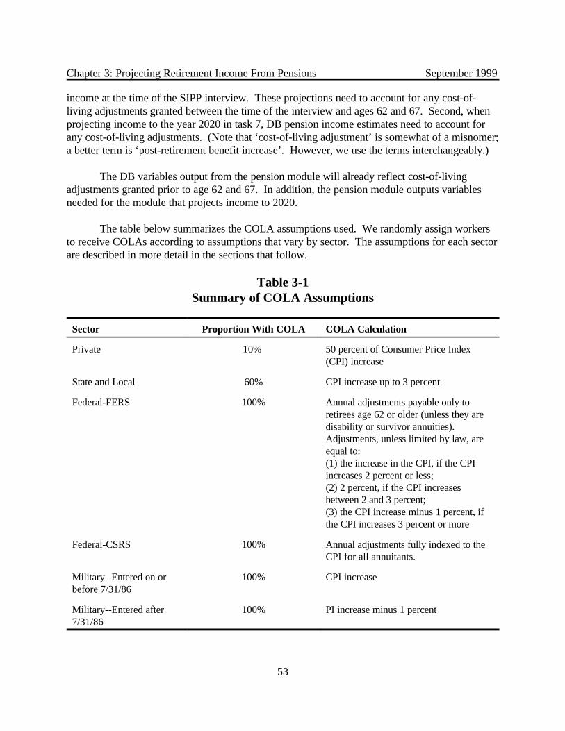
Chapter 3: Projecting Retirement Income From Pensions September 1999
53
income at the time of the SIPP interview. These projections need to account for any cost-of-living adjustments granted between the time of the interview and ages 62 and 67. Second, whenprojecting income to the year 2020 in task 7, DB pension income estimates need to account forany cost-of-living adjustments. (Note that ‘cost-of-living adjustment’ is somewhat of a misnomer;a better term is ‘post-retirement benefit increase’. However, we use the terms interchangeably.)
The DB variables output from the pension module will already reflect cost-of-livingadjustments granted prior to age 62 and 67. In addition, the pension module outputs variablesneeded for the module that projects income to 2020.
The table below summarizes the COLA assumptions used. We randomly assign workersto receive COLAs according to assumptions that vary by sector. The assumptions for each sectorare described in more detail in the sections that follow.
Table 3-1Summary of COLA Assumptions
Sector Proportion With COLA COLA Calculation
Private 10% 50 percent of Consumer Price Index(CPI) increase
State and Local 60% CPI increase up to 3 percent
Federal-FERS 100% Annual adjustments payable only toretirees age 62 or older (unless they aredisability or survivor annuities). Adjustments, unless limited by law, areequal to:(1) the increase in the CPI, if the CPIincreases 2 percent or less;(2) 2 percent, if the CPI increasesbetween 2 and 3 percent;(3) the CPI increase minus 1 percent, ifthe CPI increases 3 percent or more
Federal-CSRS 100% Annual adjustments fully indexed to theCPI for all annuitants.
Military--Entered on orbefore 7/31/86
100% CPI increase
Military--Entered after7/31/86
100% PI increase minus 1 percent

Chapter 3: Projecting Retirement Income From Pensions September 1999
54
Private Sector Employees
Although very few pension plan beneficiaries receive automatic COLAs, many receive adhoc pension increases. During the 1970s, a majority of DB beneficiaries received cost-of-livingadjustments, although most of these were granted on an ad hoc nature rather than automatically(Allen et al 1985). The post-retirement adjustments during this period amounted to about 40percent of the CPI increase.
During the 1980s, however, defined benefit plans became much less likely to grant ad hocpost-retirement increases (Allen et al, 1992, Weinstein, 1997). Part of the decline appears relatedto lower inflation; fewer plans grant increases in times of lower inflation. Even in the early 1990s,though, when inflation rates were similar to those in the late 1980s, there were further decreasesin the proportion of workers in plans which granted COLAs.
Weinstein (1997) examines the trends in the proportion of workers that are in DB plansthat granted post-retirement increases to their retirees. In 1983, 54 percent of full-time DBpension participants were in plans that either granted automatic COLAs or discretionary ad hocincreases to retirees in the last 5 years. This proportion decreased to 10 percent and 7 percent in1993 and 1995, respectively. We assume that 10 percent of all private sector DB beneficiariesreceive post-retirement benefit increases. This is slightly higher than the percentage in 1995, andwill therefore allow for a slightly higher proportion of plans that grant ad hoc increases in higherinflationary periods.
In the latest years for which information is available (1983-1988), post-retirementincreases amounted to about half of the CPI increase (Weinstein, 1997). Therefore, we assumethat post-retirement benefit increases (for those receiving them) are equal to one half of the CPIincrease. Although Weinstein (1997) finds that on average, workers with lower benefits receivehigher post-retirement increases relative to workers with higher benefits, for simplicity, we do notvary CPI increases by benefit level.
State and Local Employees
State and local employees are much more likely to receive a post-retirement benefitincrease than private sector workers. According to Weinstein (1997), 62 percent of state andlocal government workers were in plans that granted post-retirement benefit increases, themajority of which were automatic cost-of-living adjustments rather than ad hoc increases. Thehigher rate of increase among public employees is likely due in part to a higher proportion of stateand local employees not being covered by Social Security, which grants automatic COLAs. About one-quarter of state and local workers are not covered by Social Security, whereas nearlyall private sector workers are covered. It would be preferable to have separate COLAassumptions for covered and non-covered state and local workers. However, post-retirementpension increase information is not available for each group separately. Therefore, we assume

Chapter 3: Projecting Retirement Income From Pensions September 1999
55
that 60 percent of state and local workers receive post-retirement benefit increases, regardless ofwhether the worker is covered by Social Security.
Of the state and local plans that provide post-retirement benefit increases, about 60percent limit the increase to 3 percent or less per year (BLS 1988, table 69). Therefore, weassume that the state and local workers assigned to receive post-retirement benefit increasesreceive increases equal to the increase in CPI up to a maximum of 3 percent.
Federal Employees
COLA factors for federal employees are straightforward. Federal retirees receive cost-of-living adjustments according which plan they are in--FERS or CSRS.
FERS provides annual adjustments payable only to retirees age 62 or older (unless theyare disability or survivor annuities). Adjustments, unless limited by law, are equal to:
(1) the increase in the CPI, if the CPI increases 2 percent or less;(2) 2 percent, if the CPI increases between 2 and 3 percent;(3) the CPI increase minus 1 percent, if the CPI increases 3 percent or more.
CSRS provides annual adjustments fully indexed to the CPI for all annuitants.
The table below shows the actual cost-of-living adjustments for federal plans from 1990through 1997.
Table 3-2Actual COLAs for 1990-1997, Federal Plans
Month and Year of Increase FERS CSRS
January 1990January 1991January 1992January 1993April 1994April 1995April 1996January 1997
3.7%4.42.72.02.02.02.02.0
4.7%5.43.73.02.62.82.62.9
Military Personnel
COLA factors for military personnel depend on the date they entered service. Thoseentering service on or before 7/31/86 receive COLAs equal to the CPI increase. Those enteringafter 7/31/86 receive COLAs equal to the CPI increase minus one percent.

Chapter 3: Projecting Retirement Income From Pensions September 1999
56
5. Benefit Reductions for Job Changes
Few workers remain on the same job throughout their career. Workers with definedbenefit coverage who change jobs receive lower pension benefits than those who do not changejobs. This results in part because the salaries used in benefit computations are not indexed. Therefore, we adjust benefits to take into account future job changes among workers with DBcoverage. This involves two steps. First we determine who changes a job and if so how often. Second, we determine how benefits are reduced for those who change jobs.1
Determining Who Changes Jobs and How Often.
We base our estimates of who experiences a job change on the assumption that each year5 percent of workers in jobs with DB pension coverage will change jobs. This assumption isbased on Gustman and Steinmeier’s (1995) finding that the average annual rate of job changeamong male pension participants age 31-50 is 6 percent. We use a 5 percent rate rather than a 6percent rate to reflect multi-employer plans. That is, workers covered by multi-employer planswill be able to keep their DB coverage without disruption when they change jobs.
Although there is some evidence that the rate of job change is higher for some workers(e.g. younger workers, workers with shorter tenure, workers in certain industries) and lower forother workers (e.g. older workers, workers with longer tenure, workers in certain industries), forsimplicity we do not vary the job change rate by either worker or employment characteristics.
The table below shows the resulting distribution of workers across the number of jobchanges, by the number of years of service remaining in their career. (Years of service remainingis the number of years from a worker’s current age until retirement.)
Table 3-3Distribution of Workers Across Number of Job Changes
Number of Job Changes
Years of Service Remaining
35 30 25 20 15 10
0123+
16.6%30.627.425.4
21.5%33.925.918.7
27.7%36.523.012.8
35.8%37.718.9 7.6
46.3%36.613.5 3.6
59.9%31.5 7.5 1.1
We assume that all workers age 50 or older remain on their current job until retirement. We also assume that workers with fewer than 10 years of service remaining until retirementremain on their current job until retirement.

Chapter 3: Projecting Retirement Income From Pensions September 1999
57
Distribution of Job Tenure
Once we have determined how many jobs a worker has in his/her lifetime, we determinehow long the worker holds each of these jobs. We’ve decided to structure a worker’s career suchthat each job is twice as long as the job that preceded it. Two factors contributed to this decision. First, workers tend to change jobs earlier in their career rather than later. Second, the longer aperson works on his/her last job, the less changing jobs affects their total pension income.
When determining the length of each job, we ignore information on the amount of serviceto date on a worker’s present job as of the SIPP interview. Therefore, we will understate the timeon the first job if the worker has already been on the job longer than we specify through ourassumptions. For these workers, we will overstate the time on the last job, and thus, ourreductions to pension income due to job changes may be slightly understated. (On the other hand,by ignoring tenure on the current job, we could overstate the probability of job change for thosewith longer tenures, and thus overstate the reductions to pension income due to job changes.)
The table below shows the resulting years of service on each job by the number of jobchanges and years of service. (Here, the years of service is the sum of the years of serviceremaining and the years of service to date on the current job.) For instance, we assume that aworker with 35 years of service who changes jobs 3 times will work 2 years on the first job, 5years on the second, 9 years on the third, and 19 years on the fourth.
Table 3-4 Years of Service on Each Job, by Number of Job Changes
TotalYears ofService
Number of Job Changes
1 2 3
353025201510
12 years/23 years10 / 208 / 177 / 135 / 103 / 7
5 years/10 years/20 years4 / 9 / 174 / 7 / 143 / 6 / 112 / 4 / 91 / 3 / 6
2 years/5 years/9 years /19 years2 / 4 / 8 / 162 / 3 / 7 / 131 / 3 / 5 / 111 / 2 / 4 / 81 / 1 / 3 / 5
Reduction in Pension Income
We calculated pension reduction factors that are based on the total years of service (yearsof service remaining plus years of service on current job to date), the number of job changes, andoccupation. In calculating these factors we used a nominal wage growth rate of 4.4 percent. Thisassumption is based on the long-range intermediate wage growth assumption in the 1998 SocialSecurity Trustees’ Report.
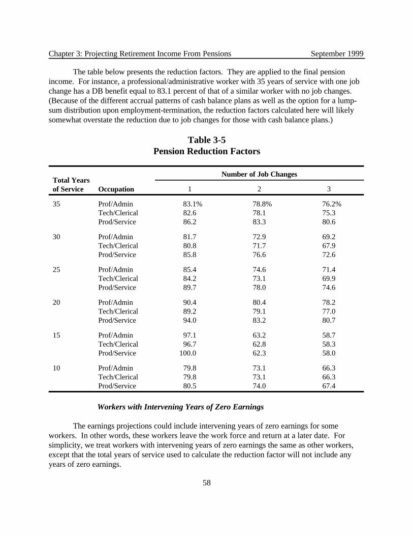
Chapter 3: Projecting Retirement Income From Pensions September 1999
58
The table below presents the reduction factors. They are applied to the final pensionincome. For instance, a professional/administrative worker with 35 years of service with one jobchange has a DB benefit equal to 83.1 percent of that of a similar worker with no job changes. (Because of the different accrual patterns of cash balance plans as well as the option for a lump-sum distribution upon employment-termination, the reduction factors calculated here will likelysomewhat overstate the reduction due to job changes for those with cash balance plans.)
Table 3-5Pension Reduction Factors
Total Yearsof Service Occupation
Number of Job Changes
1 2 3
35 Prof/AdminTech/ClericalProd/Service
83.1%82.686.2
78.8%78.183.3
76.2%75.380.6
30 Prof/AdminTech/ClericalProd/Service
81.780.885.8
72.971.776.6
69.267.972.6
25 Prof/AdminTech/ClericalProd/Service
85.484.289.7
74.673.178.0
71.469.974.6
20 Prof/AdminTech/ClericalProd/Service
90.489.294.0
80.479.183.2
78.277.080.7
15 Prof/AdminTech/ClericalProd/Service
97.196.7
100.0
63.262.862.3
58.758.358.0
10 Prof/AdminTech/ClericalProd/Service
79.879.880.5
73.173.174.0
66.366.367.4
Workers with Intervening Years of Zero Earnings
The earnings projections could include intervening years of zero earnings for someworkers. In other words, these workers leave the work force and return at a later date. Forsimplicity, we treat workers with intervening years of zero earnings the same as other workers,except that the total years of service used to calculate the reduction factor will not include anyyears of zero earnings.

Chapter 3: Projecting Retirement Income From Pensions September 1999
59
This may overstate the pension benefits for those with intervening years of zero earnings,but only for those who return to the work force in new jobs rather than returning to the same job. In any case, the projected pensions for workers with intervening years of zero earnings alreadypartly account for any job changes by using years of service that are reduced for years of zeroearnings.
6. Inclusion of Widow(er) Benefits
We include pre-retirement survivor benefits so that we do not understate the income forwidow(ers) whose spouses died prior to receiving their pension income. For workers who dieprior to age 62 (67), we determine what their pension would be at age 62 (67) if they had lefttheir job the day prior to the day they died. We assume that each of these workers would havetaken a 50 percent joint and survivor benefit. Then we assume that the surviving widow(er)begins to receive the survivor benefit when the worker would have attained age 62 (67), had he orshe lived. This last assumption is made to be consistent with our assumption that workers do notbegin to receive their pension benefits until they attain age 62 (67). For surviving spouses whostart receiving survivorship benefits prior to attainment of age 62 (67), we apply COLAadjustments up to age 62 (67), as described above.
7. Current Retirement Income
About 4 percent of persons in the projection sample are currently collecting pensionincome, with their annual pension benefit averaging about $12,000. We project current pensionincome to ages 62 and 67. We assume that everyone in this group is collecting income from a DBplan, and we randomly assign COLA increases according to the COLA methods discussed above.
We also make assumptions regarding the survivorship status of those receiving pensionbenefits. We assume that pension recipients who are not married and report that they have jointand survivor plans are in survivorship mode. For those who are married and report that they havejoint and survivor plans, we assume that they are collecting joint benefits. If a member of thecouple dies before reaching age 62 or 67, we switch the surviving spouse to survivorship modeand reduce the benefits accordingly.
8. Benefits Expected from a Prior Job
About 11 percent of the persons age 55 to 64 in the 1990 projection sample and 9 percentof those in the 1991 sample expect to receive pension benefits from a prior job. The potentialbenefits from prior pension coverage can be substantial since workers age 55 to 64 were coveredby these prior plans for an average of about 20 years.
The previous pension model already accounted for pensions from a prior job to the extent

Chapter 3: Projecting Retirement Income From Pensions September 1999
60
that these prior pension plan balances are rolled over and included in IRA balances reported in theSIPP. Unfortunately, the 1990 SIPP does not include questions regarding previous lump sumdistributions for those under age 62. In the 1991 SIPP, however, 25 percent of those ages 55-64who expect to receive a pension benefit from a prior job also indicate they previously received alump sum distribution. Of these, 38 percent claim to have rolled the distribution over. In otherwords, 10 percent (25% * 38%) of those expecting to receive pension benefits from a prior jobalso received a lump sum distribution that they then rolled over. This is probably the upper boundon any double counting that would occur if we ignore the possibility that some people who reportthey expect to receive pension income from a prior job have actually rolled over their pensionbenefits. Therefore, it is reasonable to accept this potential for double counting rather than to tryto impute the proportion of those in the 1990 SIPP who have taken and rolled over any lump sumdistributions.
For simplicity, we assume that all of those expecting benefits from a prior job have a DBplan. This is probably reasonable, since those with DC plans are more likely to be eligible for andreceive lump sum distributions. To calculate benefits at age 62 and 67, we use the years coveredunder the plan and the salary as of the quit date (using earnings information from the earningsprojection module) and apply the appropriate replacement rate as discussed above.
III. DEFINED CONTRIBUTION (DC) PLAN AND IRA ESTIMATES
The model separately projects account balances for 401(k) plans, non-401(k) DC plans,Keoghs, and IRAs. In general, the output variables for DC plans include 401(k), non-401(k) DCplans, and Keogh plans, but not IRA plans; IRA plan output variables are displayed separately. For plans where account balance information is available, the balance is projected to theretirement date. In addition, monthly contributions are accumulated from the time of the surveyuntil the time of retirement. These contributions reflect the reported employee contribution rates,assigned employer match rates, and earnings projections. For plans where account balanceinformation is not available, monthly contributions are accumulated over the entire period of planparticipation.
The model assumes that account balances are invested 50 percent in stocks and 50 percentin bonds. Similarly, it assumes that new contributions are allocated 50 percent to stocks and 50percent to bonds. Separate rates of return are applied to the stock and bond balances andcontributions. The real rates of return are set stochastically. In future versions of the model, itmight be desirable to allow for various allocation strategies by age, gender, tenure, and/or income,and to allow for portfolio rebalancing. Time and resource constraints made it impractical toincorporate such variations in this version of the model. The Employee Benefit ResearchInstitute/ICF (EBRI/ICF) database on 401(k) plans is a potential source for informing this type ofenhancement.

Chapter 3: Projecting Retirement Income From Pensions September 1999
61
Upon the pre-retirement death of a worker, we transfer the DC account balance to thespouse.
We annuitize account balances upon attainment of age 62 (67) under two sets of mortalityassumptions. The first uses unisex mortality assumptions based on the 1989-1991 Decennial LifeTables as published by the National Center for Health Statistics (NCHS). The second set usesmortality assumptions developed by RAND and based on Panel Study of Income Dynamics(PSID) data corrected for differences between the PSID and Vital Statistics. These mortalityrates vary by gender, birth year, race, and education.
1. Employee Contribution Rates
Employee contribution rates for each account balance type (401(k), non-401(k), Keogh,and IRA) are based on self-reported SIPP data. We assume that the percentage contributed toeach plan remains a constant percentage of earnings until retirement. We might want to relax thisassumption in future versions of the model, and allow contributions to vary by age, gender,tenure, and/or income.
2. Employer Match Rates
The SIPP does not ascertain employer match rate information. We estimate match ratesfor 401k and non-401k DC plans separately.
401(k) Plans
Using the 1995 Survey of Consumer Finances (SCF), we examined employer andemployee contribution rates for 401(k) plans. We found that the employer match decreases withincreases in the employee contribution rate. This is consistent with Papke (1997) who finds thatworker contribution rates decrease as the employer match increases.
Therefore, we vary employer match rates by the worker contribution rate. For those caseswhere we do not know whether the employer contributes, we randomly assign employer matchrates based on the following distribution:
Table 3-6Distribution of Workers by Employer Match Rate
Worker Contribution Rate 0% Match 50% Match 100% Match
0.01-5.00%5.01%+
20%20%
20%60%
60%20%

Chapter 3: Projecting Retirement Income From Pensions September 1999
62
For those cases where we know whether the employer contributes, we randomly assignemployer match rates to those workers whose employer contributes using the followingdistribution:
Table 3-7Distribution of Workers by Employer Match Rate
Worker Contribution Rate 0% Match 50% Match 100% Match
0.01-5.00%5.01%+
nana
25%75%
75%25%
For workers who do not contribute toward their 401(k) plan, we assume an employercontribution rate of 5 percent of salary.
Non-401(k) Plans
We also used the SCF to examine employee and employer contribution rates for non-401(k) contribution plans. Similar to our findings for 401(k) plans, we found that employermatch rates for non-401(k) plans vary by the worker contribution rate. Accordingly, we varyemployer match rates by the worker contribution rate. For those cases where we do not knowwhether the employer contributes, we randomly assign employer match rates based on thefollowing distribution:
Table 3-8Distribution of Workers by Employer Match Rate
Worker Contribution Rate 0% Match 50% Match 100% Match
0.01-4.00%4.01-8.00%8.01%+
25%10%40%
25%40%40%
50%50%20%
For those cases where we know whether the employer contributes, we randomly assignemployer match rates to those workers whose employer contributes using the followingdistribution:

Chapter 3: Projecting Retirement Income From Pensions September 1999
63
Table 3-9Distribution of Workers by Employer Match Rate
Worker Contribution Rate 0% Match 50% Match 100% Match
0.01-4.00%4.01-8.00%8.01%+
nanana
33%44%67%
67%56%33%
For workers who do not contribute to their non-401(k) DC plan, we assume an employercontribution rate of 4.5 percent of salary.
3. Rate of Return on Account Balances
We assume that account balances reported at the time of the SIPP survey are allocatedevenly between stocks and bonds and also that new contributions are allocated evenly betweenstocks and bonds. Based on input from ORES, we assume a CPI growth rate of 3.50 percent, areal rate of return for stocks of 6.98 percent, and a real rate of return for bonds of 3.00 percent. We subtract one percent from each of the stock and bond real rates of return to reflectadministrative costs. This is the same administrative fee assumption used in the Advisory Councilreport for the intermediate return PSA-401(k) plan (1997, vol. 1, page 171). (The pensionmodule programs are structured so that the rates of return can be easily modified.) We apply thestock rate of return to the stock allocations and the bond rate of return to the bond allocations. We vary the investment experience by individual and by year by setting the rates stochastically(i.e., drawing them from a normal distribution). Based on recommendations from RAND, weassume a standard deviation of 17.28 percent for stocks and 2.14 percent for bonds.
4. Annuitization Assumptions
Upon reaching age 62 (67), we calculate annuitized account balances for everyone. Theseannuitized benefits represent the annual benefits available if the workers choose to annuitize, andtherefore, are merely illustrative. When projecting income in the years past age 62 and 67, DCpension wealth is included with non-pension wealth and the decline in wealth is estimated by age. See Chapter 7 of this report for more detail on how wealth and income is projected past ages 62and 67.
We produce two sets of annuitized benefits. The first set uses unisex mortalityassumptions based on the 1989-1991 Decennial Life Tables, as published by the NCHS. Presumably, these would be the rates appropriate under a mandated annuitization scenario. Thecode has the ability to reduce benefits by a loading factor, which is currently set at 20 percent.

Chapter 3: Projecting Retirement Income From Pensions September 1999
64
The second set uses mortality assumptions developed by RAND and based on PSID datacorrected for differences between the PSID and Vital Statistics. These mortality rates vary bygender, birth year, race, and education. The idea here is that we are simulating withdrawals fromthe account balance rather than assuming the people actually use their account balances topurchase annuities. However, because we assume that people are risk averse, we assume thatpeople will withdraw less from their DC account in order to save in case they live longer than theyexpect. Therefore, we reduce the annualized benefit that results from the annuity factorcalculations by 20 percent to reflect this risk aversion. The annuity program was written such thatthis reduction factor can be easily modified.
Regardless of which set of assumptions are used, the estimates of annuitized benefitsreflect joint and survivor annuities for married persons. The amount payable to the survivor iscurrently set at 50 percent, but can easily be modified.
5. Transfer of Account Balances to Widow(er)s
We transfer the account balances of workers who die prior to age 62 (67) to theirsurviving spouses. The account balances continue to accrue interest until the surviving spouseattains age 62 (67), but no additional contributions are made. When the surviving spouse attainsage 62 (67), the account balance is annuitized. If the surviving spouse is already age 62 (67) orolder, we annuitize the balance as of the date of the worker’s death.
IV. INCREASING FUTURE DB AND DC PENSION PLANPARTICIPATION
Some workers who are not currently covered by a pension plan (either because they arenot participating or their employer does not offer a pension) will move into DB or DC pensionplans over time. In particular, pension plan participation increases with age (up to age 50 or so)and with earnings. We randomly increase future pension participation so that it incorporatescurrent trends in pension participation by age and earnings.
Using data from the 1990-1993 SIPP, we created the following matrices of pension planparticipation rates by age, gender, and income quintile (determined by gender).
Over time, workers move from one participation rate cell to another as they age andpossibly earn more income. As non-participating workers move from one cell to another, werandomly assign them to pension plans such that the overall participation rate for the cell ispreserved. (Since we increase pension coverage among nonparticipants only, we avoid having toaddress whether new coverage replaces or supplements already existing coverage.)

Chapter 3: Projecting Retirement Income From Pensions September 1999
65
Table 3-10Pension Plan Participation Rates
Earnings Quintile
First Second Third Fourth Fifth
Men
Age 30-32Age 33-37Age 38-42Age 43-47Age 48-52Age 53-57Age 58-62
19283539424135
34455357605853
51626973757469
62727881838278
68788386878683
Women
Age 30-32Age 33-37Age 38-42Age 43-47Age 48-52Age 53-57Age 58-62
15222528262522
25333841393733
43535760585653
59687275737269
68768082817977
We use the following formula to assign pension plan coverage to non-participatingworkers:
(participation rateage in x years, earnings quintile in x years - participation ratecurrent age and earnings quintile) _______________________________________________________________
(100-participation ratecurrent age and earnings quintile)
where current age and earnings quintile are those as of the time of the SIPP survey.
For instance, 45 percent of 35 year old working men with earnings in the second quintileparticipate in a pension plan. This means that 55 percent do not participate. If in five years,however, the workers who did not participate had earnings in the third quintile and are now age40, they are now included with the group that participates at a rate of 69 percent. Therefore, (69-45)/55=44% of these workers would become new pension participants at age 40.
We compare participation rates in five year intervals until the worker reaches age 53 orolder. In other words, a 35 year old who is not participating at the time of the SIPP survey firsthas the opportunity to newly participate in a pension plan at age 40. If we do not assign coverageat age 40, the worker has another opportunity to newly participate at age 45, and then again atage 50.
Chapter 3: Projecting Retirement Income From Pensions September 1999
66
Note that we do not include any explicit cohort effects in assigning participation rates. Inother words, we assume that current 35 year olds will have the same participation rate at age 50as current 50 year olds in the same position in the earnings distribution. However, the futurepension participation rates of more recent cohorts will differ from those of current older cohortsto the extent that their earnings distributions differ.
Consistent with current trends in pension plan coverage, we assume that two-thirds of newpension participants join DC plans and one-third join DB plans. (This assumption can be easilymodified within the pension module.)
It is also possible that individuals who are not working at the time of the SIPP surveyeventually enter the labor force and participate in an employment-based pension plan. To allowfor this possibility, we apply the rates in the above pension participation matrix to thoseindividuals who according to the earnings projections, enter the work force. Take for example, awoman who is not working at age 33 but subsequently enters the labor force at age 38. Weassign her a 38 percent probability of having pension coverage, the same probability as similarlysituated women. Again, we assume that two-thirds of new participants join DC plans and one-third join DB plans.
V. RESULTS
Tables 3-11 through 3-24 summarize the output of the pension module. Tables 3-11 and3-12 present the coverage rates and mean balance and benefit amounts by various characteristicsfor the age 62 and age 67 scenarios, respectively. Tables 3-13 through 3-17 present coveragerates by birth cohort, AIME quintile, gender, and retirement age scenario. Table 3-18 presentsthe mean DB benefits by birth cohort, AIME quintile, gender, and age retirement age scenario. Similarly, Tables 3-19 through 3-21 present mean DC balances and annuitized benefits, andTables 3-22 through 3-24 present mean IRA balances and annuitized benefits.
Note that under the age 62 scenario, all benefit coverage percentages and mean balanceand benefit amounts reflect coverage and amounts at age 62 assuming retirement andannuitization by age 62. Similarly, under the age 67 scenario, all benefit coverage percentagesand mean balance and benefit amounts reflect coverage and amounts at age 67 assumingretirement and annuitization by age 67. In these tables, mean balances and benefits reflect thosefor persons with coverage only.
1. Pension Coverage
The left panel of Table 3-11 presents pension coverage rates under the retirement age 62scenario. Coverage rates represent the proportion of people in the SIPP sample who will receivepension benefits at age 62. Forty-seven percent have pension coverage from a DB or DC

Chapter 3: Projecting Retirement Income From Pensions September 1999
67
(including Keoghs) plan. In addition, 20 percent have IRA coverage. Overall, 62 percent havepension coverage from any source at age 62 (including DB, DC, and IRA coverage).
The Income of the Aged Chartbook, 1996 (SSA ORES, 1998, p. 8) shows that 41 percentof aged units receive retirement benefits other than Social Security (includes private pensions andannuities, government employee pensions, railroad retirement, and IRA, Keogh, and 401(k)payments). Our percentages are higher by about 20 percentage points, presumably because weinclude all persons with DC and IRA account balances, regardless of whether they will actuallyreceive annuitized benefits. (Note also that the Chartbook uses aged units, whereas we look atpersons.)
The left panel of Table 3-12 presents pension coverage rates under the retirement age 67scenario. The overall proportion of persons receiving pension income is slightly higher under theage 67 scenario; overall coverage rates including IRA coverage are 63 percent under the age 67scenario and 62 percent under the age 62 scenario. However, coverage for each type of plan islower under the age 67 scenario. For example, DB coverage is 35 percent under the age 62scenario and 33 percent under the age 67 scenario. This suggests that there are fewer people withmultiple plan types under the age 67 scenario then there are under the age 62 scenario.
Regardless of the retirement age scenario used, some pension coverage patterns emerge. Although overall coverage rates are roughly similar by birth cohort, overall rates mask thedifferences by plan type. For instance, IRA coverage is lower among more recent cohorts,primarily because we have chosen not to assign future IRA coverage to those not currentlyparticipating in an IRA plan. However, since those with IRA coverage typically also have eitherDB or DC coverage, this does not change overall coverage rates by cohort. In addition, DBcoverage decreases and DC coverage increases among more recent cohorts. This results, in part,from our assumptions regarding new coverage. Our future pension participation module assumesthat two-thirds of new pension plan participants are in a DC plan. We feel this is appropriategiven current trends in plan types.
Pension coverage increases with lifetime income, as measured by one’s AIME as a portionof national average wages in the year one turns age 62 (67). Persons in the highest AIME quintilehave pension coverage rates over twice those in the first quintile. In addition, men are more likelyto have pension coverage than women, although participation in IRAs is nearly identical. Pensioncoverage is higher for married persons, those with more education, and whites and non-Hispanics.

Chapter 3: Projecting Retirement Income From Pensions September 1999
68
Coverage
DB Benefit DC Balance DC Benefit DC Benefit IRA Balance IRA Benefit IRA BenefitDB, DC, or IRA IRA DB or DC DB DC (unisex mort) (indiv mort) (unisex mort) (indiv mort)
ALL 61.5% 20.2% 47.2% 34.6% 21.0% 0.281 5.671 0.444 0.403 1.411 0.110 0.100
AIME QuintileQuintile 1 37.0 13.7 25.6 21.3 7.6 0.386 4.155 0.325 0.292 0.882 0.069 0.062 Quintile 2 45.0 14.2 32.1 24.8 10.8 0.153 2.783 0.218 0.196 1.443 0.112 0.101 Quintile 3 61.5 15.3 47.6 33.8 19.7 0.168 3.032 0.239 0.217 1.494 0.117 0.106 Quintile 4 75.9 22.1 59.8 42.4 27.2 0.246 4.801 0.377 0.343 1.490 0.117 0.106 Quintile 5 88.2 35.8 70.8 50.5 39.8 0.406 8.699 0.679 0.618 1.514 0.118 0.107
Birth Cohort<1931 59.5 32.4 45.6 41.6 7.4 0.474 1.653 0.127 0.119 0.008 0.001 0.001 1931-1935 62.5 32.8 46.5 39.0 15.6 0.416 2.298 0.177 0.166 0.119 0.009 0.009 1936-1940 62.4 27.8 45.2 34.6 20.6 0.355 3.263 0.251 0.235 0.522 0.040 0.038 1941-1945 63.2 24.7 46.9 34.8 22.7 0.294 4.451 0.346 0.317 1.012 0.079 0.072 1949-1950 64.7 22.1 49.2 35.6 24.1 0.265 5.598 0.436 0.398 1.619 0.126 0.114 1951-1955 62.5 17.9 47.8 33.5 23.8 0.230 6.181 0.484 0.440 2.342 0.183 0.166 1956-1960 60.6 13.5 47.5 32.6 22.9 0.199 7.543 0.592 0.534 3.114 0.242 0.219 1961-1965 57.6 8.3 46.7 30.9 21.9 0.174 7.030 0.555 0.498 3.609 0.284 0.255
GenderFemale 57.2 19.8 44.8 32.8 19.2 0.216 4.983 0.394 0.344 1.466 0.116 0.102 Male 66.5 20.6 49.6 36.4 22.9 0.341 6.276 0.487 0.455 1.355 0.105 0.098
Marital StatusSingle 60.2 13.8 39.1 29.4 17.0 0.258 5.982 0.466 0.419 1.777 0.138 0.123 Married 62.1 24.1 52.1 37.8 23.5 0.292 5.531 0.434 0.396 1.281 0.100 0.092
EducationHS dropout 37.0 6.2 28.4 22.5 8.4 0.188 2.595 0.202 0.203 0.513 0.040 0.040 HS grad 60.2 17.5 46.3 34.2 19.9 0.246 4.710 0.369 0.340 1.310 0.102 0.094 College 78.5 34.9 60.6 42.7 31.1 0.376 7.624 0.596 0.531 1.627 0.127 0.113
RaceWhite 63.2 22.3 48.0 35.0 21.8 0.287 5.790 0.453 0.411 1.396 0.109 0.099 Black 51.0 5.5 42.3 33.2 15.2 0.246 4.211 0.330 0.310 1.639 0.128 0.120 Native 52.6 9.3 42.9 32.3 16.2 0.206 4.066 0.318 0.289 1.240 0.096 0.087 Asian 54.3 17.1 42.7 29.8 20.4 0.235 6.403 0.503 0.453 1.667 0.130 0.117
HispanicNo 63.1 21.4 48.3 35.4 21.7 0.285 5.723 0.448 0.407 1.410 0.110 0.100 Yes 43.1 6.4 34.9 25.1 13.8 0.208 4.766 0.373 0.345 1.448 0.113 0.103
Pension TypeNo pension - - - - - na na na na na na naIRA only 100.0 100.0 - - - na na na na 1.102 0.087 0.079 DC only 100.0 - 100.0 - 100.0 na 5.408 0.426 0.388 na na naDC and IRA 100.0 100.0 100.0 - 100.0 na 7.457 0.585 0.523 2.050 0.158 0.144 DB only 100.0 - 100.0 100.0 - 0.234 na na na na na naDB and IRA 100.0 100.0 100.0 100.0 - 0.369 na na na 1.131 0.088 0.080 DB and DC 100.0 - 100.0 100.0 100.0 0.289 4.529 0.352 0.324 na na naDB DC and IRA 100.0 100.0 100.0 100.0 100.0 0.393 6.139 0.476 0.432 1.872 0.146 0.131
SIPP Wave1990 61.0 19.7 46.2 32.1 22.2 0.278 6.069 0.475 0.431 1.650 0.129 0.117 1991 62.6 20.0 47.8 36.2 19.5 0.277 5.082 0.397 0.362 1.457 0.113 0.103 1992 62.5 20.1 49.0 37.7 19.3 0.274 5.181 0.406 0.369 1.418 0.111 0.100 1993 59.9 20.9 45.6 32.3 23.0 0.296 6.194 0.484 0.440 1.133 0.089 0.080
Note:1. AIME Quintile Breaks are: 0.192, 0.498, 0.836, and 1.273 times the national average wage.
Benefit and Balance Means (as a percentage of average national wage)Employment-Based
Table 3-11 Pension Coverage Rates and Mean Benefits and Balances, Age 62 Scenario

Chapter 3: Projecting Retirement Income From Pensions September 1999
69
Coverage
Employment-Based DB Benefit DC Balance DC Benefit DC Benefit IRA Balance IRA Benefit IRA BenefitDB, DC, or IRA IRA DB or DC DB DC (unisex mort) (indiv mort) (unisex mort) (indiv mort)
ALL 62.5% 19.2% 44.7% 32.9% 19.9% 0.258 7.391 0.648 0.569 2.052 0.180 0.157
AIME QuintileQuintile 1 38.5 13.4 25.5 21.3 7.7 0.380 6.085 0.534 0.462 1.446 0.128 0.110 Quintile 2 45.6 13.3 30.8 24.1 10.1 0.144 3.723 0.327 0.280 2.018 0.179 0.153 Quintile 3 63.2 14.8 46.5 33.2 19.5 0.155 4.232 0.373 0.325 2.222 0.196 0.170 Quintile 4 76.9 21.2 56.0 40.0 25.5 0.219 6.324 0.557 0.490 2.223 0.195 0.171 Quintile 5 88.4 32.5 63.2 45.3 35.7 0.369 11.078 0.968 0.853 2.118 0.185 0.162
Birth Cohort<1931 61.8 31.9 44.3 40.3 7.6 0.416 2.545 0.221 0.196 0.162 0.014 0.013 1931-1935 64.5 30.7 43.2 36.4 14.8 0.379 3.866 0.337 0.304 0.543 0.048 0.043 1936-1940 63.5 26.0 43.0 33.4 19.6 0.343 4.714 0.407 0.368 1.051 0.092 0.082 1941-1945 64.0 23.5 44.2 32.9 21.4 0.276 6.129 0.532 0.474 1.615 0.141 0.125 1949-1950 65.4 20.9 46.4 33.9 22.7 0.249 7.255 0.632 0.559 2.348 0.206 0.179 1951-1955 63.2 16.9 45.1 31.9 22.3 0.213 7.905 0.694 0.610 3.255 0.286 0.247 1956-1960 61.2 12.8 45.0 31.1 21.7 0.181 9.486 0.833 0.727 4.118 0.362 0.312 1961-1965 58.3 7.9 44.3 29.5 20.6 0.157 9.012 0.800 0.688 4.529 0.402 0.344
GenderFemale 58.6 19.4 44.4 32.8 19.1 0.205 6.741 0.599 0.500 2.252 0.200 0.168 Male 67.4 18.9 44.9 33.1 20.7 0.314 8.017 0.695 0.635 1.836 0.159 0.145
Marital StatusSingle 61.7 12.9 35.1 26.6 15.2 0.242 7.807 0.678 0.587 2.619 0.228 0.194 Married 62.9 24.4 52.6 38.2 23.8 0.267 7.169 0.632 0.559 1.801 0.159 0.140
EducationHS dropout 38.2 5.9 26.2 20.9 7.7 0.170 3.428 0.297 0.294 0.814 0.071 0.070 HS grad 61.1 16.7 43.9 32.7 18.9 0.227 6.061 0.532 0.475 1.894 0.167 0.148 College 78.8 32.9 57.5 40.8 29.5 0.344 10.025 0.879 0.753 2.374 0.208 0.177
RaceWhite 64.2 21.2 45.5 33.3 20.7 0.264 7.554 0.662 0.580 2.041 0.179 0.156 Black 52.2 5.3 39.9 31.3 14.3 0.228 5.388 0.474 0.433 2.224 0.195 0.179 Native 53.5 8.1 39.7 30.7 13.9 0.200 5.230 0.461 0.410 1.885 0.163 0.142 Asian 55.4 16.1 40.7 28.7 19.1 0.223 8.298 0.732 0.634 2.220 0.195 0.168
HispanicNo 64.1 20.3 45.7 33.8 20.5 0.262 7.445 0.653 0.572 2.049 0.180 0.157 Yes 44.3 6.2 32.8 23.7 13.0 0.196 6.448 0.563 0.505 2.130 0.187 0.165
Pension TypeNo pension - - - - - na na na na na na naIRA only 100.0 100.0 - - - na na na na 1.570 0.139 0.122 DC only 100.0 - 100.0 - 100.0 na 6.919 0.608 0.539 na na naDC and IRA 100.0 100.0 100.0 - 100.0 na 9.723 0.852 0.741 2.826 0.248 0.215 DB only 100.0 - 100.0 100.0 - 0.214 na na na na na naDB and IRA 100.0 100.0 100.0 100.0 - 0.334 na na na 1.605 0.141 0.124 DB and DC 100.0 - 100.0 100.0 100.0 0.264 5.823 0.511 0.452 na na naDB DC and IRA 100.0 100.0 100.0 100.0 100.0 0.371 8.322 0.728 0.628 2.931 0.257 0.220
SIPP Wave1990 62.1 18.5 43.5 30.6 20.8 0.255 7.890 0.693 0.608 2.396 0.211 0.183 1991 63.8 19.2 45.2 34.4 18.4 0.253 6.823 0.598 0.525 2.001 0.176 0.153 1992 63.4 19.2 46.6 36.0 18.4 0.255 6.808 0.597 0.524 2.145 0.188 0.164 1993 60.8 19.8 43.3 30.9 21.9 0.270 7.883 0.691 0.606 1.689 0.149 0.129
Note:1. AIME Quintile Breaks are: 0.192, 0.498, 0.836, and 1.273 times the national average wage.
Benefit and Balance Means (as a proportion of average national wage)
Table 3-12Pension Coverage Rates and Mean Benefits and Balances, Age 67 Scenario

Chapter 3: Projecting Retirement Income From Pensions September 1999
70
Table 3-13 through 3-17 present coverage rates (DB/DC/IRA, IRA, DB/DC, DB, andDC) by birth cohort, gender, AIME quintile, and retirement age scenario. Among women, thepercentage with pension coverage from any source (including IRAs) remains fairly steady acrosscohorts (Table 3-13). However, an interesting trend emerges when examining the percentage ofwomen with either DB or DC coverage (Table 3-14). Although coverage rates by birth cohortremain fairly steady within AIME quintiles, coverage rates increase for more recent cohorts in theaggregate. This likely reflects a shift in the distribution of women by AIME quintile; women inmore recent birth cohorts are more likely to be in higher AIME quintiles, and therefore are morelikely to have pension coverage. This trend is consistent with Johnson (1999), who concludesthat the gender gap in pension coverage is due primarily to gender differences in income.
Among men, the percentage with pension coverage from any source (including IRAs)decreases slightly, both within AIME quintiles and overall (Table 3-13). Decreases within thelowest two AIME quintiles are more dramatic than those in the higher AIME quintile, suggestingthat low lifetime earners in more recent cohorts are relatively worse off than low lifetime earnersin older cohorts. Similar trends are evident when examining the percentage of men with eitherDB or DC coverage (Table 3-14).
When examining DB coverage in particular, coverage rates hold steady for women bybirth cohort (although in general, rates decrease by cohort within AIME quintiles) and decreasefor men by birth cohort, both within AIME quintiles and overall (Table 3-15). DC coverage ratesincrease by cohort, for both men and women, both overall and within AIME quintiles (Table 3-16). Again, however, these trends in overall coverage rates by coverage type reflect ourassumption that two-thirds of new pension participants will be in DC plans. Finally, IRAcoverage decreases by birth cohort for both women and men, both within AIME quintiles andoverall, reflecting that we do not assign future IRA coverage to those not currently participatingin an IRA plan (Table 3-17).
2. DB Benefits
The right panels of Tables 3-11 and 3-12 present the mean benefits and balances for thevarious pension types. Note again that means are for those with coverage only. Mean DBbenefits are 0.28 times and 0.26 times the national average salary, under the age 62 and age 67scenarios, respectively. Benefits are slightly lower under the age 67 scenario because workers aremore likely to leave their job prior to age 67 than they are to leave prior to age 62. Because finalsalaries used in DB benefit computations are not indexed, leaving a job prior to age 62 (67) willresult in lower benefits.
In general, patterns of DB benefits are similar to those in pension plan coverage. Amongthose receiving DB benefits, average DB benefits are higher among men, married persons, moreeducated persons, whites, and non-hispanics. Although DB benefits increase from AIME

Chapter 3: Projecting Retirement Income From Pensions September 1999
71
Percentage with DB, DC, or IRA Coverage at 62, by Birth Cohort and AIME QuintileAge 62 Scenario
1931- 1936- 1941- 1946- 1951- 1956-ALL <1931 1935 1940 1945 1950 1955 1960 1961+
ALL ALL 62 59 62 62 63 65 63 61 58AIME QuintileQuintile 1 37 39 41 39 38 40 37 32 30Quintile 2 45 54 52 50 48 45 39 42 41Quintile 3 61 61 67 64 63 62 63 61 57Quintile 4 76 77 73 73 75 79 78 76 74Quintile 5 88 90 89 89 89 90 88 87 85
Female ALL 57 50 56 56 58 60 59 58 57AIME QuintileQuintile 1 34 36 38 35 34 35 34 32 29Quintile 2 48 56 54 52 53 48 43 43 42Quintile 3 70 71 78 77 71 71 69 68 65Quintile 4 84 87 88 84 87 87 84 82 78Quintile 5 90 92 89 93 91 92 89 89 89
Male ALL 66 70 70 70 69 70 67 64 59AIME QuintileQuintile 1 47 54 58 60 54 55 43 32 35Quintile 2 38 46 47 42 36 34 30 41 39Quintile 3 50 50 52 46 49 48 54 52 47Quintile 4 71 75 68 68 68 72 74 71 70Quintile 5 88 90 89 88 89 89 88 86 83
Percentage with DB, DC, or IRA Coverage at 67, by Birth Cohort and AIME QuintileAge 67 Scenario
1931- 1936- 1941- 1946- 1951- 1956-ALL <1931 1935 1940 1945 1950 1955 1960 1961+
ALL ALL 63 62 65 64 64 65 63 61 58AIME QuintileQuintile 1 38 41 44 42 40 41 38 33 32Quintile 2 46 56 53 50 49 45 40 42 42Quintile 3 63 63 70 65 64 64 64 63 59Quintile 4 77 77 75 75 76 80 79 77 75Quintile 5 88 91 89 89 90 90 88 87 85
Female ALL 59 53 58 58 59 61 60 59 58AIME QuintileQuintile 1 36 37 41 37 36 36 35 33 30Quintile 2 48 58 54 52 53 49 44 43 43Quintile 3 71 74 79 76 71 72 71 70 67Quintile 4 84 86 89 85 86 87 84 82 80Quintile 5 90 95 91 93 91 92 90 89 87
Male ALL 67 72 72 71 70 70 67 64 59AIME QuintileQuintile 1 49 58 60 62 56 56 46 34 38Quintile 2 38 48 50 43 35 33 29 40 39Quintile 3 52 49 55 46 51 51 55 55 49Quintile 4 72 75 69 70 69 74 75 72 70Quintile 5 88 91 89 88 90 89 88 85 83
Birth Cohort
Birth Cohort
Table 3-13Percentage with DB, DC, or IRA Coverage

Chapter 3: Projecting Retirement Income From Pensions September 1999
72
Percentage with DB or DC Coverage at 62, by Birth Cohort and AIME QuintileAge 62 Scenario
1931- 1936- 1941- 1946- 1951- 1956-ALL <1931 1935 1940 1945 1950 1955 1960 1961+
ALL ALL 47 46 47 45 47 49 48 47 47AIME QuintileQuintile 1 26 25 25 24 25 29 27 25 24Quintile 2 32 40 37 35 32 31 27 31 32Quintile 3 48 50 52 46 48 48 48 48 45Quintile 4 60 63 57 54 59 60 61 61 61Quintile 5 71 74 73 71 69 71 70 70 72
Female ALL 45 35 39 40 43 48 47 48 49AIME QuintileQuintile 1 23 20 20 19 21 25 26 25 24Quintile 2 34 40 36 36 35 34 31 33 34Quintile 3 57 56 62 59 56 58 56 58 56Quintile 4 72 73 76 70 75 75 72 72 70Quintile 5 80 86 78 80 78 82 79 78 82
Male ALL 50 58 55 51 51 51 48 47 45AIME QuintileQuintile 1 35 50 47 46 40 42 30 24 26Quintile 2 27 39 39 30 25 23 20 27 29Quintile 3 36 43 39 30 35 34 37 37 35Quintile 4 53 62 51 47 50 51 54 53 54Quintile 5 68 73 73 70 67 68 67 67 67
Percentage with DB or DC Coverage at 67, by Birth Cohort and AIME QuintileAge 67 Scenario
1931- 1936- 1941- 1946- 1951- 1956-ALL <1931 1935 1940 1945 1950 1955 1960 1961+
ALL ALL 45 44 43 43 44 46 45 45 44AIME QuintileQuintile 1 26 24 25 25 25 29 27 24 25Quintile 2 31 40 33 33 31 29 26 30 32Quintile 3 47 48 50 44 46 46 47 48 45Quintile 4 56 58 52 51 55 57 57 57 56Quintile 5 63 69 63 63 62 64 63 63 63
Female ALL 44 36 39 40 43 47 47 47 48AIME QuintileQuintile 1 23 20 22 21 22 25 26 25 24Quintile 2 34 40 33 35 34 33 31 32 35Quintile 3 57 56 59 56 56 58 56 58 56Quintile 4 69 71 72 66 70 71 69 69 68Quintile 5 76 80 75 77 75 77 76 74 78
Male ALL 45 54 48 46 46 46 44 43 40AIME QuintileQuintile 1 33 48 39 43 37 37 30 22 25Quintile 2 25 37 33 28 22 20 17 25 27Quintile 3 34 37 37 28 32 32 37 37 34Quintile 4 48 55 44 44 46 48 49 48 47Quintile 5 60 68 62 61 59 60 58 58 56
Birth Cohort
Birth Cohort
Table 3-14Percentage with DB or DC Coverage

Chapter 3: Projecting Retirement Income From Pensions September 1999
73
Percentage with DB Coverage at 62, by Birth Cohort and AIME QuintileAge 62 Scenario
1931- 1936- 1941- 1946- 1951- 1956-ALL <1931 1935 1940 1945 1950 1955 1960 1961+
ALL ALL 35 42 39 35 35 36 34 33 31AIME QuintileQuintile 1 21 23 22 20 20 24 22 20 20Quintile 2 25 36 30 27 24 22 20 24 25Quintile 3 34 45 43 34 34 33 33 32 30Quintile 4 42 58 47 41 43 42 41 40 37Quintile 5 51 65 60 53 51 51 48 46 44
Female ALL 33 32 32 30 32 35 34 34 33AIME QuintileQuintile 1 19 19 17 15 17 20 21 20 20Quintile 2 26 36 29 27 26 24 22 26 25Quintile 3 40 50 51 42 42 39 38 38 37Quintile 4 50 66 61 53 52 54 49 48 43Quintile 5 56 78 60 63 56 63 55 52 51
Male ALL 36 53 47 39 38 37 33 31 29AIME QuintileQuintile 1 29 48 43 39 32 34 24 19 19Quintile 2 22 36 35 25 19 17 15 20 23Quintile 3 26 40 33 24 24 25 26 26 23Quintile 4 38 57 43 36 38 35 35 34 33Quintile 5 49 65 61 52 50 48 46 44 41
Percentage with DB Coverage at 67, by Birth Cohort and AIME QuintileAge 67 Scenario
1931- 1936- 1941- 1946- 1951- 1956-ALL <1931 1935 1940 1945 1950 1955 1960 1961+
ALL ALL 33 40 36 33 33 34 32 31 29AIME QuintileQuintile 1 21 23 21 21 20 23 22 20 20Quintile 2 24 36 28 26 23 22 20 23 24Quintile 3 33 43 42 33 34 32 33 32 29Quintile 4 40 53 43 40 41 41 39 38 35Quintile 5 45 62 52 48 45 46 43 41 39
Female ALL 33 32 32 31 32 34 33 33 33AIME QuintileQuintile 1 19 19 18 18 18 21 21 20 20Quintile 2 26 36 28 27 25 24 23 25 26Quintile 3 40 49 49 41 43 39 39 38 37Quintile 4 49 63 58 52 47 50 49 47 43Quintile 5 53 71 56 60 55 59 52 49 48
Male ALL 33 50 41 36 34 33 30 29 26AIME QuintileQuintile 1 27 46 36 37 29 30 23 17 19Quintile 2 20 35 29 23 17 16 13 18 22Quintile 3 25 35 31 22 21 23 26 26 22Quintile 4 35 51 38 34 37 34 33 31 29Quintile 5 43 61 52 46 43 43 40 38 35
Birth Cohort
Birth Cohort
Table 3-15Percentage with DB Coverage

Chapter 3: Projecting Retirement Income From Pensions September 1999
74
Percentage with DC Coverage at 62, by Birth Cohort and AIME QuintileAge 62 Scenario
1931- 1936- 1941- 1946- 1951- 1956-ALL <1931 1935 1940 1945 1950 1955 1960 1961+
ALL ALL 21 7 16 21 23 24 24 23 22AIME QuintileQuintile 1 8 3 6 8 9 11 9 8 6Quintile 2 11 7 12 14 13 12 11 10 9Quintile 3 20 8 17 21 22 22 21 20 20Quintile 4 27 10 18 24 27 30 31 31 32Quintile 5 40 17 31 38 40 40 42 44 45
Female ALL 19 5 13 18 20 23 23 22 21AIME QuintileQuintile 1 6 2 5 6 7 9 8 7 6Quintile 2 12 6 12 15 14 13 13 10 10Quintile 3 25 10 21 29 25 28 26 26 25Quintile 4 36 17 27 34 40 41 37 36 37Quintile 5 47 16 39 41 47 45 50 49 50
Male ALL 23 10 19 24 26 25 25 24 22AIME QuintileQuintile 1 12 5 8 19 17 16 13 10 8Quintile 2 9 7 11 9 11 8 8 10 8Quintile 3 14 5 10 11 17 14 15 14 15Quintile 4 22 8 15 19 20 24 27 27 28Quintile 5 38 17 31 38 39 39 40 42 43
Percentage with DC Coverage at 67, by Birth Cohort and AIME QuintileAge 67 Scenario
1931- 1936- 1941- 1946- 1951- 1956-ALL <1931 1935 1940 1945 1950 1955 1960 1961+
ALL ALL 20 8 15 20 21 23 22 22 21AIME QuintileQuintile 1 8 3 6 9 9 10 9 8 6Quintile 2 10 6 10 13 12 11 10 10 9Quintile 3 20 8 16 20 21 22 21 20 20Quintile 4 25 10 17 22 25 29 28 29 29Quintile 5 36 15 28 34 37 37 39 39 40
Female ALL 19 6 13 17 19 22 22 21 21AIME QuintileQuintile 1 7 3 6 6 8 9 8 7 5Quintile 2 11 6 10 14 13 12 12 10 11Quintile 3 25 11 20 28 25 28 26 26 24Quintile 4 34 18 27 30 37 38 35 34 35Quintile 5 46 20 40 43 46 44 49 47 48
Male ALL 21 9 17 22 23 23 22 22 20AIME QuintileQuintile 1 11 5 7 18 16 14 12 10 9Quintile 2 8 6 9 8 10 6 6 9 7Quintile 3 13 4 11 10 16 14 15 14 15Quintile 4 20 8 13 19 18 22 24 25 25Quintile 5 33 15 27 33 35 35 35 36 36
Birth Cohort
Birth Cohort
Table 3-16Percentage with DC Coverage

Chapter 3: Projecting Retirement Income From Pensions September 1999
75
Percentage with IRA Coverage at 62, by Birth Cohort and AIME QuintileAge 62 Scenario
1931- 1936- 1941- 1946- 1951- 1956-ALL <1931 1935 1940 1945 1950 1955 1960 1961+
ALL ALL 20 32 33 28 25 22 18 13 8AIME QuintileQuintile 1 14 23 24 20 16 13 10 6 3Quintile 2 14 28 27 23 19 15 11 9 4Quintile 3 15 27 30 24 21 16 14 10 7Quintile 4 22 38 32 30 26 24 20 16 10Quintile 5 36 63 56 44 40 37 33 26 20
Female ALL 20 29 31 28 24 22 18 14 8AIME QuintileQuintile 1 14 23 24 19 16 14 10 6 3Quintile 2 17 31 29 26 22 18 13 10 5Quintile 3 20 35 40 33 26 21 17 12 8Quintile 4 27 53 48 44 35 32 25 19 12Quintile 5 36 66 55 50 43 41 38 34 23
Male ALL 21 36 35 28 26 22 18 13 8AIME QuintileQuintile 1 12 22 26 22 17 13 9 4 2Quintile 2 8 16 20 11 10 10 5 7 3Quintile 3 9 18 16 14 13 9 9 7 5Quintile 4 20 35 27 24 21 18 17 14 9Quintile 5 36 63 56 43 39 36 31 24 18
Percentage with IRA Coverage at 67, by Birth Cohort and AIME QuintileAge 67 Scenario
1931- 1936- 1941- 1946- 1951- 1956-ALL <1931 1935 1940 1945 1950 1955 1960 1961+
ALL ALL 19 32 31 26 24 21 17 13 8AIME QuintileQuintile 1 13 22 24 19 16 13 9 6 3Quintile 2 13 25 25 21 18 15 11 8 4Quintile 3 15 28 27 22 20 16 13 10 6Quintile 4 21 36 31 29 26 23 19 15 10Quintile 5 32 58 48 38 36 34 30 24 18
Female ALL 19 29 30 27 23 22 18 13 8AIME QuintileQuintile 1 14 22 24 19 16 13 10 6 3Quintile 2 16 29 27 24 22 17 14 10 5Quintile 3 20 37 36 31 25 20 17 12 8Quintile 4 26 50 47 42 34 31 23 18 11Quintile 5 35 57 52 47 39 40 36 32 23
Male ALL 19 35 31 25 24 20 16 12 7AIME QuintileQuintile 1 11 22 23 21 15 13 9 5 2Quintile 2 7 14 18 11 9 8 4 6 2Quintile 3 9 16 15 11 14 9 9 7 5Quintile 4 18 32 24 23 21 17 16 13 9Quintile 5 32 58 48 37 35 32 27 21 15
Birth Cohort
Birth Cohort
Table 3-17Percentage with IRA Coverage

Chapter 3: Projecting Retirement Income From Pensions September 1999
76
quintile two up to AIME quintile five, average DB benefits for those in the lowest AIME quintileare nearly that of those in the highest AIME quintile. This counterintuitive result might becaused, in part, by workers who are not covered by Social Security. These noncovered workerswill have an AIME of zero, but will actually have nonzero lifetime earnings, and since they aremost likely to be government workers, they will have generous DB benefits. This could beartificially increasing the mean benefits of those in AIME quintile one. Average DB benefitsamong those receiving benefits decrease by birth cohort, for both women and men, within AIMEquintiles and overall (Table 3-18).
Average DB benefits are lower among more recent cohorts, which likely reflects themethod of projecting earnings. Earnings are projected based on a single-equation approach (usingearnings of persons reporting both positive earnings as well as those with zero earnings in givenyears) rather than a two-equation approach (the first equation estimates whether individuals havepositive covered earnings; the second estimates the level of earnings for those with earnings). Asa result of using the single-equation approach, earnings in later years will be understated for manyindividuals who continue to work and will be overstated for those who stop working.
Since DB benefits rely on the earnings projections to estimate final salary (defined in theDB pension model as the highest five consecutive years of earnings out of the last 10 years ofearnings), any over- or understatements in earnings will affect DB benefit levels. For olderworkers who continue working, the final salary used in the DB benefit estimation may be too low,and therefore their benefits may be understated. Any understatement of benefits will beconcentrated among the more recent cohorts because the potential for understating earningsamong older workers increases for more recent cohorts.
For those who left the labor force prior to reaching age 62 or 67, the single-equationapproach can result in several years of low, rather than zero, earnings at the end of a worker’scareer. Although this method may overstate earnings later in life, the final salary may actually beunderstated because it will reflect the artificially low earnings rather than the actual earnings thatpreceded labor force departure. Since the single-equation method may overstate the number ofyears of service, however, it is unclear whether the DB benefits will be over- or understated forthose who leave the labor force prior to age 62 or 67.
3. DC Balances and Potential Annuitized Benefits
Average DC balances under the retirement age 62 scenario are 5.67 times the nationalaverage wage (Table 3-11, middle panel). There is a 30 percent increase in DC balances from theage 62 scenario to the age 67 scenario, when balances are 7.39 times the national average salary. This is due in part to additional contributions between age 62 and 67. However, it is probablyprimarily due to our investment assumptions. The combination of a 50 percent stock/50 percentbond allocation of initial account balances and future contributions along with the higher rates of

Chapter 3: Projecting Retirement Income From Pensions September 1999
77
DB Benefit at 62 (as a Proportion of National Average Wages), by Birth Cohort and AIME QuintileAge 62 Scenario
1931- 1936- 1941- 1946- 1951- 1956-ALL <1931 1935 1940 1945 1950 1955 1960 1961+
ALL ALL 0.28 0.47 0.42 0.36 0.29 0.27 0.23 0.20 0.17 AIME QuintileQuintile 1 0.39 0.52 0.50 0.55 0.50 0.42 0.35 0.19 0.09 Quintile 2 0.15 0.32 0.30 0.21 0.16 0.14 0.09 0.08 0.07 Quintile 3 0.17 0.36 0.29 0.21 0.16 0.14 0.12 0.12 0.12 Quintile 4 0.25 0.43 0.37 0.29 0.22 0.21 0.19 0.19 0.19 Quintile 5 0.41 0.72 0.56 0.48 0.40 0.36 0.34 0.34 0.33
Female ALL 0.22 0.32 0.28 0.25 0.22 0.22 0.21 0.18 0.16 AIME QuintileQuintile 1 0.26 0.36 0.33 0.35 0.32 0.28 0.26 0.14 0.08 Quintile 2 0.11 0.19 0.18 0.13 0.10 0.11 0.09 0.08 0.07 Quintile 3 0.16 0.29 0.22 0.17 0.15 0.14 0.13 0.13 0.13 Quintile 4 0.24 0.48 0.41 0.29 0.23 0.21 0.21 0.20 0.20 Quintile 5 0.40 0.97 0.56 0.55 0.41 0.39 0.39 0.36 0.34
Male ALL 0.34 0.58 0.52 0.44 0.36 0.31 0.25 0.22 0.19 AIME QuintileQuintile 1 0.64 0.84 0.84 0.91 0.87 0.63 0.53 0.32 0.11 Quintile 2 0.26 0.70 0.64 0.46 0.34 0.24 0.08 0.09 0.06 Quintile 3 0.19 0.47 0.42 0.29 0.18 0.15 0.10 0.10 0.10 Quintile 4 0.25 0.42 0.35 0.30 0.21 0.20 0.16 0.17 0.18 Quintile 5 0.41 0.71 0.56 0.47 0.39 0.34 0.33 0.33 0.32
DB Benefit at 67 (as a Proportion of National Average Wages), by Birth Cohort and AIME QuintileAge 67 Scenario
1931- 1936- 1941- 1946- 1951- 1956-ALL <1931 1935 1940 1945 1950 1955 1960 1961+
ALL ALL 0.26 0.42 0.38 0.34 0.28 0.25 0.21 0.18 0.16 AIME QuintileQuintile 1 0.38 0.47 0.48 0.57 0.50 0.43 0.36 0.19 0.09 Quintile 2 0.14 0.29 0.29 0.20 0.15 0.15 0.09 0.08 0.06 Quintile 3 0.15 0.31 0.26 0.21 0.16 0.14 0.11 0.11 0.11 Quintile 4 0.22 0.35 0.34 0.27 0.21 0.19 0.17 0.17 0.17 Quintile 5 0.37 0.62 0.49 0.43 0.36 0.32 0.31 0.31 0.31
Female ALL 0.20 0.29 0.27 0.25 0.21 0.21 0.20 0.17 0.15 AIME QuintileQuintile 1 0.26 0.34 0.34 0.36 0.32 0.28 0.26 0.14 0.08 Quintile 2 0.11 0.18 0.18 0.13 0.10 0.12 0.09 0.08 0.07 Quintile 3 0.15 0.24 0.20 0.17 0.14 0.13 0.12 0.12 0.12 Quintile 4 0.22 0.39 0.35 0.25 0.22 0.19 0.20 0.19 0.19 Quintile 5 0.37 0.78 0.57 0.46 0.36 0.35 0.36 0.34 0.33
Male ALL 0.31 0.51 0.47 0.43 0.34 0.29 0.23 0.20 0.16 AIME QuintileQuintile 1 0.65 0.74 0.83 1.00 0.91 0.70 0.57 0.34 0.11 Quintile 2 0.24 0.65 0.62 0.46 0.35 0.26 0.08 0.08 0.06 Quintile 3 0.17 0.43 0.40 0.30 0.19 0.16 0.10 0.08 0.09 Quintile 4 0.22 0.34 0.33 0.29 0.20 0.19 0.14 0.15 0.15 Quintile 5 0.37 0.61 0.48 0.43 0.36 0.30 0.29 0.29 0.29
Birth Cohort
Birth Cohort
Table 3-18 DB Benefit

Chapter 3: Projecting Retirement Income From Pensions September 1999
78
return for stocks means that by the time people reach retirement age, a majority of their accountbalances are invested in stocks. This, in turn, means that a greater proportion of their accountsreceive the higher stock rates of return. In future revisions to this module, it may be preferable toassume periodic portfolio re-balancing.
Regardless of the retirement age scenario, DC balances are higher for men, single persons,more educated persons, whites and Asians, and non-Hispanics. DC balances are somewhat higherfor AIME quintile one then for quintile two, and then increase steadily from quintile two throughquintile five. DC balances are also higher among younger birth cohorts, primarily because of thestock/bond allocation assumptions mentioned above. More recent cohorts have had more time toaccumulate their balances, and therefore, have an even higher proportion of their portfoliosinvested in stocks (with their higher rate of return) by retirement age than do older cohorts. Thus,in the aggregate, while projected DB benefits among more recent cohorts may be biaseddownward, there could be an offsetting upward bias in projected DC balances.
We calculated potential annuitized DC benefits per dollar of DC balances using twomortality assumptions. The first assumes a unisex mortality under the 1989-1991 Decennial LifeTables, as published by the NCHS. The second set uses mortality assumptions developed byRAND and based on PSID data corrected for differences between the PSID and Vital Statistics. These mortality rates vary by gender, birth year, race, and education. We refer to these as thegroup-specific mortality assumptions.
Under the age 62 scenario, average annuitized DC benefits are 0.44 and 0.40 times thenational average salary using the unisex and group-specific mortality assumptions, respectively. The benefits under the group-specific mortality assumptions are lower than those under the unisexmortality assumptions because under the group-specific mortality assumptions, mortality isexpected to improve over time. The unisex mortality assumptions do not include a cohort effect,resulting in higher mortality rates, and therefore, higher benefits because they are expected to bepaid over a shorter period of time.
The use of group-specific annuity rates exacerbates the differences in mean DC benefits bygender. Women’s longer life expectancies translate into lower annual benefits. Although use ofthe group-specific annuity rates appears to narrow the differences in mean DC benefits byeducation and race, these results might also reflect correlations between education, race, andgender.
Annuitized benefits under the age 67 scenario are greater than those under the age 62scenario for two reasons. First, the account balances are greater. Second, the shorter lifeexpectancy at age 67 results in higher benefits.

Chapter 3: Projecting Retirement Income From Pensions September 1999
79
In general, DC balances and annuitized benefits increase for younger birth cohorts for bothwomen and men, both overall and within AIME cohorts (Tables 3-19 through 3-21). Asmentioned above, more recent cohorts have more time to accumulate their balances, andtherefore, have an even higher proportion of their portfolios invested in stocks (with their higherrate of return) by retirement age than do older cohorts.
4. IRA Balances and Potential Annuitized Benefits
Average IRA balances are only one-quarter of those for DC plans. Average IRA balancesare 1.41 and 2.10 times the national average wage under the age 62 and age 67 scenarios,respectively. Similar to the DC balances, there is a large increase from the age 62 scenario to theage 67 scenario, likely due primarily to our investment assumptions.
Potential average IRA annuitized benefits under the age 62 scenario are 0.11 and 0.10times the national average wage, under the unisex and individual mortality assumptions,respectively. Benefits under the age 67 scenario are almost two-thirds greater, reflecting largeraccount balances and shorter life expectancies.
IRA balances and annuitized benefits increase for younger birth cohorts for both womenand men, both overall and within AIME cohorts (Tables 3-22 through 3-24). This reflects thelonger period of time that more recent cohorts can contribute toward their IRA plans.
VI. SUMMARY OF IMPROVEMENTS OVER PREVIOUS MODEL
Much of the pension benefit model builds off of the previous pension model developed aspart of the SIPP/DPE model. We enumerate the major improvements to the model below.
1. Replacement Rates by Occupation. The previous pension model variedreplacement rates by years of service in the plan, final salary, age at retirement, andsector of employment, but not by occupation. We refined the replacement ratesused so that they also account for differences by occupation. For instance, bluecollar workers are likely to have flat dollar pension benefits that do not vary byfinal earnings. Therefore, their replacement rates decrease as final earningsincrease. In contrast, white collar workers are more likely to have replacementrates that either do not vary or increase with final earnings.
2. Earnings. Earnings used to calculate DB benefits and those used to calculate DC,Keogh, and IRA contributions reflect the new earnings projections.

Chapter 3: Projecting Retirement Income From Pensions September 1999
80
DC Balance at 62 (as a Proportion of National Average Wages), by Birth Cohort and AIME QuintileAge 62 Scenario
1931- 1936- 1941- 1946- 1951- 1956-ALL <1931 1935 1940 1945 1950 1955 1960 1961+
ALL ALL 5.67 1.65 2.30 3.26 4.45 5.60 6.18 7.54 7.03 AIME QuintileQuintile 1 4.16 1.54 2.56 3.79 5.23 4.29 5.26 4.74 2.38 Quintile 2 2.78 1.01 1.38 1.64 2.55 4.51 2.91 3.08 3.01 Quintile 3 3.03 1.59 1.88 2.23 2.75 2.69 3.03 3.62 3.69 Quintile 4 4.80 1.72 1.87 3.23 3.26 4.03 4.89 6.59 6.12 Quintile 5 8.70 2.04 3.09 4.22 6.18 8.37 9.45 11.73 12.08
Female ALL 4.98 1.90 2.14 2.81 4.03 4.45 5.32 6.77 6.06 AIME QuintileQuintile 1 3.79 2.18 2.67 3.15 5.23 4.02 3.74 4.79 2.29 Quintile 2 2.65 0.83 1.35 1.57 2.78 3.57 3.00 3.11 2.91 Quintile 3 3.08 1.90 2.16 2.31 3.05 2.69 3.13 3.56 3.77 Quintile 4 5.28 2.86 2.35 4.24 3.76 4.42 5.15 7.33 5.93 Quintile 5 9.77 6.03 3.60 3.99 6.72 7.63 9.74 12.16 11.79
Male ALL 6.28 1.49 2.41 3.61 4.79 6.65 6.97 8.25 8.00 AIME QuintileQuintile 1 4.75 0.22 2.22 4.68 5.23 4.70 7.30 4.66 2.54 Quintile 2 3.19 1.48 1.47 1.99 1.77 8.69 2.58 3.02 3.20 Quintile 3 2.93 0.92 1.10 1.94 2.07 2.70 2.84 3.74 3.58 Quintile 4 4.36 1.27 1.60 2.49 2.73 3.62 4.64 5.87 6.32 Quintile 5 8.35 1.91 3.05 4.25 6.07 8.61 9.32 11.54 12.24
DC Balance at 67 (as a Proportion of National Average Wages), by Birth Cohort and AIME QuintileAge 67 Scenario
1931- 1936- 1941- 1946- 1951- 1956-ALL <1931 1935 1940 1945 1950 1955 1960 1961+
ALL ALL 7.39 2.54 3.87 4.71 6.13 7.25 7.91 9.49 9.01AIME QuintileQuintile 1 6.08 5.7 4.51 6.11 7.18 6.09 6.93 7.09 2.99Quintile 2 3.72 1 2.46 1.94 5.06 4.67 4.02 4.35 3.37Quintile 3 4.23 1.64 4.1 2.88 3.79 4.39 4.06 4.96 4.7Quintile 4 6.32 2.45 2.92 4.49 4.84 5.71 6.56 7.82 8.07Quintile 5 11.08 2.55 4.66 6.24 7.91 10.31 11.79 14.85 16.1
Female ALL 6.74 3.34 4.1 4.23 5.67 6.26 6.92 8.72 8.04AIME QuintileQuintile 1 5.86 7.74 4.59 5.35 6.77 6.16 5.18 7.55 3.18Quintile 2 3.76 0.69 2.56 1.74 5.76 4.44 4.27 4.7 2.93Quintile 3 4.39 1.74 4.96 3.02 4.14 4.46 3.87 5.35 4.89Quintile 4 6.88 4.21 3.73 5.96 5.14 6.72 7.29 7.84 7.95Quintile 5 12.36 4.24 5.22 7.43 7.96 9.13 11.69 15.85 16.41
Male ALL 8.02 1.92 3.66 5.12 6.54 8.23 8.89 10.24 10.07AIME QuintileQuintile 1 6.49 0.47 4.15 7.34 7.91 5.99 9.35 6.29 2.69Quintile 2 3.59 1.97 2.03 3.05 2.66 5.83 2.81 3.64 4.37Quintile 3 3.9 1.28 1.8 2.36 3.01 4.2 4.45 4.17 4.41Quintile 4 5.76 1.5 2.25 3.4 4.47 4.55 5.81 7.8 8.2Quintile 5 10.59 2.44 4.59 6.03 7.9 10.74 11.84 14.36 15.92
Birth Cohort
Birth Cohort
Table 3-19DC Balance
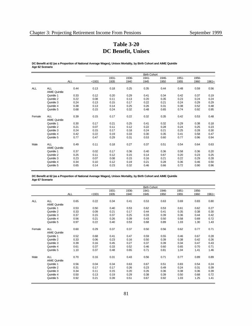
Chapter 3: Projecting Retirement Income From Pensions September 1999
81
DC Benefit at 62 (as a Proportion of National Average Wages), Unisex Mortality, by Birth Cohort and AIME QuintileAge 62 Scenario
1931- 1936- 1941- 1946- 1951- 1956-ALL <1931 1935 1940 1945 1950 1955 1960 1961+
ALL ALL 0.44 0.13 0.18 0.25 0.35 0.44 0.48 0.59 0.56 AIME QuintileQuintile 1 0.33 0.12 0.20 0.29 0.41 0.34 0.42 0.37 0.19 Quintile 2 0.22 0.08 0.11 0.13 0.20 0.35 0.23 0.24 0.24 Quintile 3 0.24 0.13 0.15 0.17 0.22 0.21 0.24 0.29 0.29 Quintile 4 0.38 0.13 0.14 0.25 0.26 0.31 0.38 0.52 0.48 Quintile 5 0.68 0.15 0.24 0.32 0.48 0.65 0.74 0.92 0.95
Female ALL 0.39 0.15 0.17 0.22 0.32 0.35 0.42 0.53 0.48 AIME QuintileQuintile 1 0.30 0.17 0.21 0.25 0.41 0.32 0.29 0.38 0.18 Quintile 2 0.21 0.07 0.11 0.12 0.22 0.28 0.24 0.25 0.23 Quintile 3 0.24 0.15 0.17 0.18 0.24 0.21 0.25 0.28 0.30 Quintile 4 0.42 0.22 0.19 0.33 0.30 0.35 0.41 0.58 0.47 Quintile 5 0.77 0.47 0.29 0.31 0.53 0.60 0.77 0.96 0.94
Male ALL 0.49 0.11 0.18 0.27 0.37 0.51 0.54 0.64 0.63 AIME QuintileQuintile 1 0.37 0.02 0.17 0.36 0.40 0.36 0.58 0.36 0.20 Quintile 2 0.25 0.11 0.12 0.15 0.14 0.67 0.20 0.23 0.25 Quintile 3 0.23 0.07 0.08 0.15 0.16 0.21 0.22 0.29 0.28 Quintile 4 0.34 0.10 0.12 0.19 0.21 0.28 0.36 0.46 0.50 Quintile 5 0.65 0.14 0.23 0.32 0.46 0.66 0.72 0.90 0.96
DC Benefit at 62 (as a Proportion of National Average Wages), Unisex Mortality, by Birth Cohort and AIME QuintileAge 67 Scenario
1931- 1936- 1941- 1946- 1951- 1956-ALL <1931 1935 1940 1945 1950 1955 1960 1961+
ALL ALL 0.65 0.22 0.34 0.41 0.53 0.63 0.69 0.83 0.80 AIME QuintileQuintile 1 0.53 0.50 0.40 0.53 0.62 0.53 0.61 0.62 0.27 Quintile 2 0.33 0.09 0.21 0.17 0.44 0.41 0.35 0.38 0.30 Quintile 3 0.37 0.15 0.37 0.25 0.33 0.39 0.36 0.44 0.42 Quintile 4 0.56 0.21 0.26 0.39 0.43 0.50 0.58 0.69 0.72 Quintile 5 0.97 0.22 0.40 0.53 0.68 0.89 1.03 1.30 1.43
Female ALL 0.60 0.29 0.37 0.37 0.50 0.56 0.62 0.77 0.71 AIME QuintileQuintile 1 0.52 0.68 0.41 0.47 0.59 0.55 0.46 0.67 0.28 Quintile 2 0.33 0.06 0.23 0.16 0.50 0.39 0.38 0.42 0.26 Quintile 3 0.39 0.16 0.45 0.27 0.37 0.39 0.34 0.47 0.43 Quintile 4 0.61 0.37 0.33 0.52 0.46 0.60 0.65 0.70 0.71 Quintile 5 1.10 0.37 0.48 0.65 0.71 0.81 1.04 1.41 1.46
Male ALL 0.70 0.16 0.31 0.43 0.56 0.71 0.77 0.89 0.89 AIME QuintileQuintile 1 0.56 0.04 0.34 0.63 0.67 0.51 0.83 0.54 0.24 Quintile 2 0.31 0.17 0.17 0.26 0.23 0.49 0.24 0.31 0.39 Quintile 3 0.34 0.11 0.15 0.20 0.26 0.36 0.38 0.36 0.39 Quintile 4 0.50 0.13 0.19 0.29 0.38 0.39 0.50 0.68 0.72 Quintile 5 0.92 0.21 0.39 0.51 0.67 0.92 1.03 1.25 1.41
Birth Cohort
Birth Cohort
Table 3-20DC Benefit, Unisex

Chapter 3: Projecting Retirement Income From Pensions September 1999
82
DC Benefit at 62 (as a Proportion of National Average Wages), Individual Mortality, by Birth Cohort and AIME QuintileAge 62 Scenario
1931- 1936- 1941- 1946- 1951- 1956-ALL <1931 1935 1940 1945 1950 1955 1960 1961+
ALL ALL 0.40 0.12 0.17 0.23 0.32 0.40 0.44 0.53 0.50 AIME QuintileQuintile 1 0.29 0.11 0.18 0.27 0.36 0.30 0.37 0.33 0.17 Quintile 2 0.20 0.07 0.10 0.12 0.18 0.32 0.20 0.22 0.21 Quintile 3 0.22 0.12 0.14 0.16 0.20 0.19 0.22 0.26 0.26 Quintile 4 0.34 0.12 0.14 0.23 0.23 0.29 0.35 0.47 0.44 Quintile 5 0.62 0.15 0.22 0.30 0.44 0.60 0.67 0.83 0.86
Female ALL 0.34 0.13 0.15 0.20 0.28 0.31 0.37 0.46 0.41 AIME QuintileQuintile 1 0.26 0.15 0.19 0.22 0.35 0.28 0.25 0.33 0.16 Quintile 2 0.18 0.06 0.10 0.11 0.19 0.25 0.21 0.21 0.19 Quintile 3 0.22 0.14 0.16 0.16 0.21 0.19 0.22 0.25 0.26 Quintile 4 0.37 0.20 0.17 0.30 0.27 0.31 0.36 0.50 0.41 Quintile 5 0.67 0.40 0.26 0.28 0.48 0.52 0.67 0.83 0.80
Male ALL 0.45 0.11 0.18 0.26 0.35 0.48 0.51 0.60 0.58 AIME QuintileQuintile 1 0.35 0.02 0.16 0.34 0.38 0.34 0.53 0.34 0.19 Quintile 2 0.24 0.11 0.11 0.15 0.13 0.66 0.19 0.22 0.23 Quintile 3 0.22 0.07 0.08 0.15 0.16 0.20 0.21 0.28 0.26 Quintile 4 0.32 0.10 0.12 0.19 0.20 0.26 0.34 0.43 0.46 Quintile 5 0.60 0.14 0.22 0.31 0.44 0.62 0.67 0.83 0.89
DC Benefit at 67 (as a Proportion of National Average Wages), Individual Mortality, by Birth Cohort and AIME QuintileAge 67 Scenario
1931- 1936- 1941- 1946- 1951- 1956-ALL <1931 1935 1940 1945 1950 1955 1960 1961+
ALL ALL 0.57 0.20 0.30 0.37 0.47 0.56 0.61 0.73 0.69 AIME QuintileQuintile 1 0.46 0.41 0.35 0.47 0.54 0.47 0.53 0.54 0.23 Quintile 2 0.28 0.08 0.19 0.16 0.37 0.35 0.30 0.33 0.25 Quintile 3 0.33 0.13 0.33 0.22 0.29 0.34 0.32 0.38 0.36 Quintile 4 0.49 0.19 0.23 0.35 0.38 0.44 0.51 0.60 0.62 Quintile 5 0.85 0.20 0.37 0.49 0.62 0.80 0.91 1.14 1.23
Female ALL 0.50 0.25 0.32 0.32 0.43 0.47 0.52 0.64 0.59 AIME QuintileQuintile 1 0.43 0.56 0.35 0.41 0.49 0.46 0.38 0.55 0.23 Quintile 2 0.28 0.05 0.20 0.14 0.42 0.33 0.31 0.34 0.21 Quintile 3 0.33 0.14 0.39 0.23 0.31 0.34 0.29 0.40 0.36 Quintile 4 0.52 0.32 0.29 0.44 0.40 0.50 0.55 0.58 0.59 Quintile 5 0.91 0.31 0.41 0.56 0.60 0.68 0.87 1.16 1.17
Male ALL 0.63 0.15 0.29 0.41 0.52 0.65 0.70 0.81 0.80 AIME QuintileQuintile 1 0.51 0.04 0.31 0.57 0.62 0.47 0.73 0.50 0.23 Quintile 2 0.29 0.16 0.17 0.24 0.22 0.47 0.23 0.29 0.35 Quintile 3 0.32 0.11 0.15 0.19 0.25 0.34 0.36 0.34 0.35 Quintile 4 0.46 0.13 0.19 0.28 0.36 0.37 0.47 0.63 0.66 Quintile 5 0.83 0.19 0.36 0.48 0.62 0.84 0.93 1.13 1.26
Birth Cohort
Birth Cohort
Table 3-21DC Benefit, Individual

Chapter 3: Projecting Retirement Income From Pensions September 1999
83
IRA Balance at 62 (as a Proportion of National Average Wages), by Birth Cohort and AIME QuintileAge 62 Scenario
1931- 1936- 1941- 1946- 1951- 1956-ALL <1931 1935 1940 1945 1950 1955 1960 1961+
ALL ALL 1.41 0.01 0.12 0.52 1.01 1.62 2.34 3.11 3.61 AIME QuintileQuintile 1 0.88 0.03 0.12 0.46 0.95 1.48 2.08 2.91 3.48 Quintile 2 1.44 - 0.10 0.49 1.06 1.69 2.34 4.53 3.28 Quintile 3 1.49 - 0.13 0.56 1.04 1.63 2.58 2.67 3.83 Quintile 4 1.49 - 0.12 0.56 1.05 1.59 2.47 3.06 3.43 Quintile 5 1.51 - 0.13 0.52 0.98 1.65 2.24 2.88 3.73
Female ALL 1.47 0.02 0.12 0.54 1.04 1.70 2.51 3.10 3.51 AIME QuintileQuintile 1 0.90 0.04 0.13 0.46 0.96 1.56 2.24 3.18 3.78 Quintile 2 1.25 - 0.10 0.50 1.02 1.67 2.43 3.03 3.59 Quintile 3 1.47 - 0.13 0.59 1.09 1.61 2.76 2.93 3.57 Quintile 4 1.82 0.01 0.11 0.64 1.13 1.73 2.77 3.42 3.24 Quintile 5 2.17 - 0.16 0.56 1.01 1.90 2.24 2.98 3.58
Male ALL 1.35 - 0.12 0.50 0.98 1.54 2.17 3.13 3.72 AIME QuintileQuintile 1 0.82 - 0.06 0.46 0.90 1.25 1.66 1.94 2.38 Quintile 2 2.37 - 0.10 0.41 1.26 1.80 1.79 8.50 2.41 Quintile 3 1.54 - 0.11 0.46 0.89 1.67 2.18 2.22 4.26 Quintile 4 1.24 - 0.13 0.50 0.98 1.44 2.18 2.70 3.61 Quintile 5 1.34 - 0.12 0.52 0.98 1.57 2.24 2.82 3.82
IRA Balance at 67 (as a Proportion of National Average Wages), by Birth Cohort and AIME QuintileAge 67 Scenario
1931- 1936- 1941- 1946- 1951- 1956-ALL <1931 1935 1940 1945 1950 1955 1960 1961+
ALL ALL 2.05 0.16 0.54 1.05 1.62 2.35 3.25 4.12 4.53 AIME QuintileQuintile 1 1.45 0.29 0.55 0.97 1.47 2.16 2.79 4.26 4.13 Quintile 2 2.02 0.11 0.52 0.96 1.70 2.37 3.79 4.26 4.39 Quintile 3 2.22 0.13 0.64 1.11 1.78 2.51 3.54 3.80 4.67 Quintile 4 2.22 0.13 0.53 1.11 1.63 2.50 3.52 4.09 4.66 Quintile 5 2.12 0.13 0.52 1.07 1.56 2.26 2.92 4.20 4.45
Female ALL 2.25 0.21 0.58 1.11 1.73 2.54 3.62 4.51 4.65 AIME QuintileQuintile 1 1.47 0.33 0.58 0.98 1.47 2.34 3.03 4.57 4.13 Quintile 2 2.01 0.10 0.54 0.98 1.67 2.41 3.92 4.20 4.74 Quintile 3 2.28 0.14 0.67 1.19 1.91 2.71 3.79 4.08 4.89 Quintile 4 2.70 0.19 0.55 1.32 1.88 2.74 4.04 4.79 4.83 Quintile 5 3.05 0.16 0.62 1.22 1.71 2.46 3.16 4.80 4.35
Male ALL 1.84 0.12 0.50 0.98 1.50 2.13 2.85 3.68 4.39 AIME QuintileQuintile 1 1.35 0.08 0.40 0.92 1.45 1.68 2.21 3.23 4.10 Quintile 2 2.07 0.16 0.44 0.75 1.91 2.14 2.91 4.44 3.23 Quintile 3 2.07 0.11 0.51 0.83 1.43 1.94 2.99 3.27 4.30 Quintile 4 1.81 0.11 0.52 0.93 1.40 2.20 3.00 3.40 4.49 Quintile 5 1.84 0.13 0.51 1.04 1.52 2.18 2.81 3.85 4.52
Birth Cohort
Birth Cohort
Table 3-22IRA Balance

Chapter 3: Projecting Retirement Income From Pensions September 1999
84
IRA Balance at 62 (as a Proportion of National Average Wages), by Birth Cohort and AIME QuintileAge 62 Scenario
1931- 1936- 1941- 1946- 1951- 1956-ALL <1931 1935 1940 1945 1950 1955 1960 1961+
ALL ALL 1.41 0.01 0.12 0.52 1.01 1.62 2.34 3.11 3.61 AIME QuintileQuintile 1 0.88 0.03 0.12 0.46 0.95 1.48 2.08 2.91 3.48 Quintile 2 1.44 - 0.10 0.49 1.06 1.69 2.34 4.53 3.28 Quintile 3 1.49 - 0.13 0.56 1.04 1.63 2.58 2.67 3.83 Quintile 4 1.49 - 0.12 0.56 1.05 1.59 2.47 3.06 3.43 Quintile 5 1.51 - 0.13 0.52 0.98 1.65 2.24 2.88 3.73
Female ALL 1.47 0.02 0.12 0.54 1.04 1.70 2.51 3.10 3.51 AIME QuintileQuintile 1 0.90 0.04 0.13 0.46 0.96 1.56 2.24 3.18 3.78 Quintile 2 1.25 - 0.10 0.50 1.02 1.67 2.43 3.03 3.59 Quintile 3 1.47 - 0.13 0.59 1.09 1.61 2.76 2.93 3.57 Quintile 4 1.82 0.01 0.11 0.64 1.13 1.73 2.77 3.42 3.24 Quintile 5 2.17 - 0.16 0.56 1.01 1.90 2.24 2.98 3.58
Male ALL 1.35 - 0.12 0.50 0.98 1.54 2.17 3.13 3.72 AIME QuintileQuintile 1 0.82 - 0.06 0.46 0.90 1.25 1.66 1.94 2.38 Quintile 2 2.37 - 0.10 0.41 1.26 1.80 1.79 8.50 2.41 Quintile 3 1.54 - 0.11 0.46 0.89 1.67 2.18 2.22 4.26 Quintile 4 1.24 - 0.13 0.50 0.98 1.44 2.18 2.70 3.61 Quintile 5 1.34 - 0.12 0.52 0.98 1.57 2.24 2.82 3.82
IRA Balance at 67 (as a Proportion of National Average Wages), by Birth Cohort and AIME QuintileAge 67 Scenario
1931- 1936- 1941- 1946- 1951- 1956-ALL <1931 1935 1940 1945 1950 1955 1960 1961+
ALL ALL 2.05 0.16 0.54 1.05 1.62 2.35 3.25 4.12 4.53 AIME QuintileQuintile 1 1.45 0.29 0.55 0.97 1.47 2.16 2.79 4.26 4.13 Quintile 2 2.02 0.11 0.52 0.96 1.70 2.37 3.79 4.26 4.39 Quintile 3 2.22 0.13 0.64 1.11 1.78 2.51 3.54 3.80 4.67 Quintile 4 2.22 0.13 0.53 1.11 1.63 2.50 3.52 4.09 4.66 Quintile 5 2.12 0.13 0.52 1.07 1.56 2.26 2.92 4.20 4.45
Female ALL 2.25 0.21 0.58 1.11 1.73 2.54 3.62 4.51 4.65 AIME QuintileQuintile 1 1.47 0.33 0.58 0.98 1.47 2.34 3.03 4.57 4.13 Quintile 2 2.01 0.10 0.54 0.98 1.67 2.41 3.92 4.20 4.74 Quintile 3 2.28 0.14 0.67 1.19 1.91 2.71 3.79 4.08 4.89 Quintile 4 2.70 0.19 0.55 1.32 1.88 2.74 4.04 4.79 4.83 Quintile 5 3.05 0.16 0.62 1.22 1.71 2.46 3.16 4.80 4.35
Male ALL 1.84 0.12 0.50 0.98 1.50 2.13 2.85 3.68 4.39 AIME QuintileQuintile 1 1.35 0.08 0.40 0.92 1.45 1.68 2.21 3.23 4.10 Quintile 2 2.07 0.16 0.44 0.75 1.91 2.14 2.91 4.44 3.23 Quintile 3 2.07 0.11 0.51 0.83 1.43 1.94 2.99 3.27 4.30 Quintile 4 1.81 0.11 0.52 0.93 1.40 2.20 3.00 3.40 4.49 Quintile 5 1.84 0.13 0.51 1.04 1.52 2.18 2.81 3.85 4.52
Birth Cohort
Birth Cohort
Table 3-23IRA Benefit, Unisex
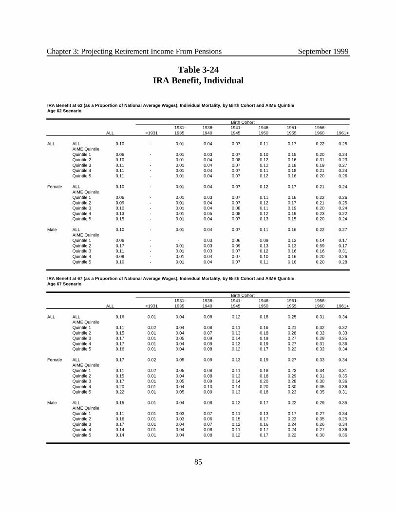
Chapter 3: Projecting Retirement Income From Pensions September 1999
85
IRA Benefit at 62 (as a Proportion of National Average Wages), Individual Mortality, by Birth Cohort and AIME QuintileAge 62 Scenario
1931- 1936- 1941- 1946- 1951- 1956-ALL <1931 1935 1940 1945 1950 1955 1960 1961+
ALL ALL 0.10 - 0.01 0.04 0.07 0.11 0.17 0.22 0.25 AIME QuintileQuintile 1 0.06 - 0.01 0.03 0.07 0.10 0.15 0.20 0.24 Quintile 2 0.10 - 0.01 0.04 0.08 0.12 0.16 0.31 0.23 Quintile 3 0.11 - 0.01 0.04 0.07 0.12 0.18 0.19 0.27 Quintile 4 0.11 - 0.01 0.04 0.07 0.11 0.18 0.21 0.24 Quintile 5 0.11 - 0.01 0.04 0.07 0.12 0.16 0.20 0.26
Female ALL 0.10 - 0.01 0.04 0.07 0.12 0.17 0.21 0.24 AIME QuintileQuintile 1 0.06 - 0.01 0.03 0.07 0.11 0.16 0.22 0.26 Quintile 2 0.09 - 0.01 0.04 0.07 0.12 0.17 0.21 0.25 Quintile 3 0.10 - 0.01 0.04 0.08 0.11 0.19 0.20 0.24 Quintile 4 0.13 - 0.01 0.05 0.08 0.12 0.19 0.23 0.22 Quintile 5 0.15 - 0.01 0.04 0.07 0.13 0.15 0.20 0.24
Male ALL 0.10 - 0.01 0.04 0.07 0.11 0.16 0.22 0.27 AIME QuintileQuintile 1 0.06 - - 0.03 0.06 0.09 0.12 0.14 0.17 Quintile 2 0.17 - 0.01 0.03 0.09 0.13 0.13 0.59 0.17 Quintile 3 0.11 - 0.01 0.03 0.07 0.12 0.16 0.16 0.31 Quintile 4 0.09 - 0.01 0.04 0.07 0.10 0.16 0.20 0.26 Quintile 5 0.10 - 0.01 0.04 0.07 0.11 0.16 0.20 0.28
IRA Benefit at 67 (as a Proportion of National Average Wages), Individual Mortality, by Birth Cohort and AIME QuintileAge 67 Scenario
1931- 1936- 1941- 1946- 1951- 1956-ALL <1931 1935 1940 1945 1950 1955 1960 1961+
ALL ALL 0.16 0.01 0.04 0.08 0.12 0.18 0.25 0.31 0.34 AIME QuintileQuintile 1 0.11 0.02 0.04 0.08 0.11 0.16 0.21 0.32 0.32 Quintile 2 0.15 0.01 0.04 0.07 0.13 0.18 0.28 0.32 0.33 Quintile 3 0.17 0.01 0.05 0.09 0.14 0.19 0.27 0.29 0.35 Quintile 4 0.17 0.01 0.04 0.09 0.13 0.19 0.27 0.31 0.36 Quintile 5 0.16 0.01 0.04 0.08 0.12 0.17 0.22 0.32 0.34
Female ALL 0.17 0.02 0.05 0.09 0.13 0.19 0.27 0.33 0.34 AIME QuintileQuintile 1 0.11 0.02 0.05 0.08 0.11 0.18 0.23 0.34 0.31 Quintile 2 0.15 0.01 0.04 0.08 0.13 0.18 0.29 0.31 0.35 Quintile 3 0.17 0.01 0.05 0.09 0.14 0.20 0.28 0.30 0.36 Quintile 4 0.20 0.01 0.04 0.10 0.14 0.20 0.30 0.35 0.36 Quintile 5 0.22 0.01 0.05 0.09 0.13 0.18 0.23 0.35 0.31
Male ALL 0.15 0.01 0.04 0.08 0.12 0.17 0.22 0.29 0.35 AIME QuintileQuintile 1 0.11 0.01 0.03 0.07 0.11 0.13 0.17 0.27 0.34 Quintile 2 0.16 0.01 0.03 0.06 0.15 0.17 0.23 0.35 0.25 Quintile 3 0.17 0.01 0.04 0.07 0.12 0.16 0.24 0.26 0.34 Quintile 4 0.14 0.01 0.04 0.08 0.11 0.17 0.24 0.27 0.36 Quintile 5 0.14 0.01 0.04 0.08 0.12 0.17 0.22 0.30 0.36
Birth Cohort
Birth Cohort
Table 3-24IRA Benefit, Individual

Chapter 3: Projecting Retirement Income From Pensions September 1999
86
3. Accounting for Retirement Prior to Age 62 (67). The previous pension modelassumed that all workers continue on their current job until age 62. However,some people stop working prior to attaining age 62. Therefore, we use outputfrom the earnings projections module to take into account retirement prior to age62 (67). Rather than assuming that workers continue to work up to age 62 (67), we assume that workers work up to the time their earnings drop to zero (or untilages 62 (67), whichever comes first). Note however, that even for workers whostop working prior to age 62 (67), we assume that they do not start collecting theirpension benefits until age 62 (67).
4. Incorporating Cost-of-living Adjustments (COLAs). The prior model did notinclude any provisions for cost-of-living adjustments (COLAs). We incorporatedCOLAs for two reasons. First, in the pension projection module, we need toproject the pension income at ages 62 and 67 for persons already collectingpension income at the time of the SIPP interview. These projections need toaccount for any cost-of-living adjustments granted between the time of theinterview and ages 62 and 67. Second, when projecting income to the year 2020in Chapter 7, DB pension income estimates need to account for any cost-of-livingadjustments.
5. Accounting for Job Changes. The prior model assumed that workers will continueat their current job until retirement. However, few workers remain on the samejob throughout their career. Workers with defined benefit coverage who changejobs receive lower pension benefits than those who do not change jobs. Thisresults in part because the salaries used in benefit computations are not indexed. Therefore, we adjust benefits to take into account future job changes amongworkers with DB coverage. This involves two steps. First we determine whochanges a job and if so how often. Second, we determine how benefits arereduced for those who change jobs.
6. Inclusion of Widow(er) Benefits. The previous pension model ignored any pre-retirement survivor benefits. This understates the income for widow(er)s whosespouses died prior to receiving their pension income. We revised the model toinclude pre-retirement DB survivor benefits. We also transfer the account balancesof workers who die prior to age 62 (67) to their surviving spouses. The accountbalances continue to accrue interest until the surviving spouse attains age 62 (67),but no additional contributions are made. When the surviving spouse attains age62 (67), the account balance is annuitized. If the surviving spouse is already age62 (67) or older, we annuitize the balance as of the date of the worker’s death.

Chapter 3: Projecting Retirement Income From Pensions September 1999
87
7. Inclusion of Benefits for Older Individuals in the Sample. The prior modelaccounted for neither the current receipt of pension income nor for pensions fromprevious jobs. Both of these omissions cause pension income to be understated inthe prior SIPP/DPE model, particularly for older individuals in the SIPP file. Werevised the pension module to include these pension benefits.
8. Refined Employer Match Rates. We updated the employer match assumptions. For 401(k) plans, the previous model assumed a 50 percent match rate for allemployee contributions. For non-401(k) contributory DC plans, the previousmodel assumed a 50 percent match rate for employees who contribute less than 16percent of pay and an employer contribution of 7 percent of pay for employeeswho contribute more than 16 percent of pay (the maximum combined contributionwas set at 25 percent of pay). We refined these assumptions so that they moreclosely parallel the distribution of employer match rates.
9. Refined Rate of Return. The prior model set the rate of return stochastically withan assumed rate of 3.5 percent (a blend of stock and interest bearing rates ofreturn) and a standard deviation equal to the assumed rate. The variation accountsfor differences in investment allocation across those with DC plans. We haveupdated the model to include assumptions regarding investment allocation. Weassume that 50 percent of account balances are invested in stocks and 50 percentare invested in bonds. We also assume that 50 percent of new contributions areallocated to stocks and 50 percent are allocated to bonds. Then we apply thestock rate of return to the stock allocations and the bond rate of return to the bondallocations. We continue to set these rates stochastically (i.e., we draw them froma normal distribution).
10. Refined Annuitization Assumptions. The prior model used insurance industryannuity rates to convert DC and IRA account balances at retirement into an annualflow of annuity income. We produce two estimates of annual annuitized benefitsfrom account balances at retirement. The first uses unisex mortality assumptionsbased on the 1989-1991 Decennial Life Tables, as published by the NCHS. Thesecond uses mortality assumptions, developed by RAND based on PSID data, thatvary by gender, birth year, race, and education.
VII. POTENTIAL FUTURE IMPROVEMENTS TO THE MODEL
1. Explicitly Modeling Different Retirement Dates From DB Plans. The currentmodel assumes that individuals do not begin collecting pension benefits until age62 (67) regardless of whether they left the labor force prior to attaining this age. In future versions of the model, it may be preferable to relax this assumption,

Chapter 3: Projecting Retirement Income From Pensions September 1999
88
which would require additional coordination with the assets projection module. This modification would complement a revision of the earnings model (describedin Chapter 2) to include a more explicit projection of the retirement decisionbetween ages 55 and 61.
2. Match Actual Plan Data to SIPP Pension Plan Participants. It may be preferable touse actual plan data rather than BLS replacement rates for workers with DBcoverage. Possible data sources are the Health and Retirement Study (HRS)pension plan data and PBGC’s PIMS model.
3. Incorporate Cash Balance Plans. The current model does not incorporate cashbalance plans. It might be desirable to include cash balance plans as more data onthese plans becomes available.
4. Incorporate a More Sophisticated Job Transition Subroutine. Rather than applyingbenefit reduction rates to account for benefits lost due to job transitions, it mightbe preferable to actually simulate a work history for each worker. The probabilityof changing jobs in any given year could reflect gender, age, tenure, industry,occupation, pension coverage, etc. This option, especially when combined withthe option for matching actual pension plans to workers, could enhance themodel’s ability to estimate pension benefits for workers who change jobs.
5. Varying DC Contribution Rates and Asset Allocations Over Time. In futureversions of the model, it might be desirable to allow for various contribution ratesby age, gender, tenure, and/or income. It might also be desirable to allow forvarious allocation strategies by age, gender, tenure, and/or income, and to allowfor portfolio rebalancing. Time and resource constraints made it impractical toincorporate such variations in this version of the model. The EBRI/ICF databaseon 401(k) plans is a potential source for informing these types of enhancement.
6. Lump Sum Distributions. In the event that a worker changes jobs or leaves thework force, the model assumes that all account balances are left to accumulate. Infuture versions of the model, it might be preferable to allow workers to take lumpsum distributions. This would require coordination with the non-pension assetaccumulation module described in Chapter 4.

Chapter 3: Projecting Retirement Income From Pensions September 1999
89
CHAPTER 3: REFERENCES
1994-1996 Advisory Council on Social Security. 1997. Report of the 1994-1996 AdvisoryCouncil on Social Security, Washington, DC.
Allen, Steven, Robert Clark, and Ann McDermed. 1992. "Postretirement Benefit Increases in the1980s," in John Turner (ed.) Trends in Pensions 1992, Washington: USGPO.
Allen, Steven, Robert Clark, and Daniel Sumner. 1985. "Inflation and Pension Benefits," inRichard Ippolito and Walter Kolodrubetz (eds.) The Handbook of Pension Statistics 1985,Washington: USGPO.
Board of Trustees, Federal Old-Age and Survivors Insurance and Disability Insurance TrustFunds. 1998. The 1998 Annual Report of the Board of Trustees of the Federal Old-Ageand Survivors Insurance and Disability Insurance Trust Funds. Washington: Author.
Gustman, Alan L. and Thomas L. Steinmeier. 1995. Pension Incentives and Job Mobility,Kalamazoo, MI: W.E. Upjohn Institute for Employment Research.
Johnson, Richard W. 1999. “The Gender Gap in Pension Wealth: Is Women’s Progress in theLabor Market Equalizing Retirement Benefits?”, The Urban Institute, The RetirementProject Issue Brief Series, No. 1.
Social Security Administration Office of Research, Evaluation, and Statistics. 1996. Income ofthe Aged Chartbook. Washington: Author.
Papke, Leslie E. 1997. “Are 401(k) Plans Replacing Other Employer-Provided Pensions?Evidence from Panel Data,” mimeo.
U.S. Bureau of Labor Statistics (BLS). 1998. Employee Benefits in Medium and Large PrivateEstablishments, 1995, BLS Bulletin No. 2496.
U.S. Bureau of Labor Statistics (BLS). 1996. Employee Benefits in State and LocalGovernments, 1994, BLS Bulletin No. 2477.
U.S. Bureau of Labor Statistics (BLS). 1994. Employee Benefits in Medium and Large PrivateEstablishments, 1993, BLS Bulletin No. 2456.
U.S. Bureau of Labor Statistics (BLS). 1990. Employee Benefits in Medium and Large PrivateEstablishments, 1989, BLS Bulletin No. 2363.

Chapter 3: Projecting Retirement Income From Pensions September 1999
90
U.S. Bureau of Labor Statistics (BLS). 1988. Employee Benefits in State and LocalGovernments, 1987, BLS Bulletin No. 2309.
Weinstein, Harriet. 1997. “Post-retirement Pension Increases,” Compensation and WorkingConditions, Fall 1997.
CHAPTER 3: LIST OF TABLES
Table 3-1Summary of COLA Assumptions 53
Table 3-2Actual COLAs for 1990-1997, Federal Plans 55
Table 3-3Distribution of Workers Across Number of Job Changes 56
Table 3-4 Years of Service on Each Job, by Number of Job Changes 57
Table 3-5Pension Reduction Factors 58
Table 3-6Distribution of Workers by Employer Match Rate 61
Table 3-7Distribution of Workers by Employer Match Rate 62
Table 3-8Distribution of Workers by Employer Match Rate 62
Table 3-9Distribution of Workers by Employer Match Rate 63
Table 3-10Pension Plan Participation Rates 65
Table 3-11 Pension Coverage Rates and Mean Benefits and Balances, Age 62 Scenario 68
Table 3-12Pension Coverage Rates and Mean Benefits and Balances, Age 67 Scenario 69
Table 3-13Percentage with DB, DC, or IRA Coverage 71
Table 3-14Percentage with DB or DC Coverage 72
Table 3-15Percentage with DB Coverage 73
Table 3-16Percentage with DC Coverage 74

Chapter 3: Projecting Retirement Income From Pensions September 1999
91
1. Rather than applying benefit reduction rates to account for benefits lost due to job transitions,we considered simulating a work history for each worker, with the probability of changing jobs inany given year reflecting gender, age, tenure, industry, occupation, pension coverage, etc. Because of the time and resource constraints we chose the former option. The latter option mightbe worth considering for future versions of the model.
Table 3-17Percentage with IRA Coverage 75
Table 3-18 DB Benefit 77
Table 3-19DC Balance 80
Table 3-20DC Benefit, Unisex 81
Table 3-21DC Benefit, Individual 82
Table 3-22IRA Balance 83
Table 3-23IRA Benefit, Unisex 84
Table 3-24IRA Benefit, Individual 85
CHAPTER 3: ENDNOTES

92
CHAPTER 4
PROJECTIONS OF NON-PENSION WEALTH ANDINCOME
I. OVERVIEW
It is quite likely, given recent changes in private pension coverage and uncertainty over thecourse of future Social Security reform efforts, that personal saving will play an increasinglyimportant role in the income security of future retirees. This chapter describes the methodologyand results of our projections of non-pension assets at age 62 and 67 for individuals contained onthe merged SIPP-SER data file.
We focus separately on housing and non-housing wealth, because it is likely thatindividuals perceive a clear distinction between both forms of savings. In addition, research(Hurd, 1990; Gustman and Juster, 1996) suggests retirees are less likely to spend down housingwealth, at least in the early stages of retirement. Calculation of the income flows associated withthese asset stocks are described in Chapter 7 of this report.
The existing economic literature on why people save is theoretically sophisticated, withmost research based on applications of the life-cycle hypothesis (LCH) (Modigliani andBrumberg, 1954). But empirical evidence on the LCH is mixed and no theory does a very goodjob of explaining data on wealth trajectories. While both demographic characteristics (race,education, marriage, divorce, and number of children) and income levels affect rates of wealthaccumulation, the data reveal substantial heterogeneity in wealth at retirement among individualswith similar demographic characteristics and earnings histories. This makes the development ofequations that provide reliable projections of future wealth accumulation a daunting task.
To project wealth of individuals for the MINT project, we developed an equation toexplain non-pension wealth as a function of age, demographic characteristics of individuals, andeconomic and demographic variables (marital status, earnings history, and availability of apension) projected in earlier stages of the project. This equation was then used to project wealthat ages 62 and 67 for individuals in the 1990-93 SIPP files. In keeping with the overallmethodology of the MINT project, all of the wealth figures presented are relative to the averagenational wage in the particular year for which the projections were made and the results areshown on an individual (per person) basis. To derive individual wealth for married couples, eachspouse was allocated one half of estimated total family wealth. Finally, the projection equationswere calibrated to actual wealth data on the 1990-93 SIPP files, so that the difference between

93
reported wealth of any individual on the SIPP file and predicted wealth of that individual at thecorresponding age was treated as an individual-specific error term. This error term was then usedto adjust the predictions of wealth at ages 62 and 67.
The outline of this chapter is as follows. The next section describes our overall approachand data sources used in the estimates and projections and then summarizes the methodology forestimation, calibration, and projection of wealth at ages 62 and 67. The following sectionpresents our econometric estimates for wealth at ages 62 and 67. The final section presents theresults of our projections of wealth at ages 62 and 67, based on the econometric estimates andcalibration to data on the 1990-93 SIPP files, and discusses qualifications and potentialimprovements. Two appendicies present the results of alternative econometric specifications.
II. METHODOLOGY
1. Overall Approach and Data Sources
Selection of Overall Approach
We considered two overall approaches to projecting lifetime wealth accumulation patternsof future retirees. The first approach relied on the simulation of annual consumption decisions,deriving wealth at retirement as the cumulative outcome of annual saving (income minusconsumption) and rates of return on assets. This approach was rejected on a number of grounds,including a concern that it would not be feasible to simulate such complex processes in the verytight time-frame of the MINT project. Also, it was believed that this approach presumed aknowledge of saving behavior that does not exist.
The second approach, which was the one we selected, used a reduced-form equation toestimate the wealth of individuals as a function of age, earnings histories, and demographiccharacteristics. The resulting age-wealth profiles reflect the combined effects of decisions on howmuch to save, portfolio allocations, and realized rates of return on assets. While this approach hasless detail than the first approach on the process of wealth accumulation, it does allowstraightforward estimation of the pattern of wealth changes over the life cycle.
In deriving age-wealth profiles, we developed separate econometric estimates andprojections for housing and non-housing wealth. We define housing wealth as the differencebetween home value and outstanding mortgage debt (i.e., home equity). Non-housing, non-pension wealth is calculated as the sum of the net value of: vehicles, other real estate, farm andbusiness equity (value - debt), stocks, mutual funds, bonds, checking accounts, savings accounts,money market accounts, and certificate of deposit account balances, less unsecured debt.

Chapter 4: Projections of Non-Pension Wealth and Income September 1999
94
Choice of Panel Survey of Income Dynamics (PSID) for Estimates
In performing these estimates, we utilized longitudinal data from the Panel Study onIncome Dynamics (PSID). We chose the PSID instead of the Survey of Income and ProgramParticipation (SIPP) to perform this estimation because the PSID enables us to observe thewealth-generating process for an individual over a longer period (approximately ten years) thanthe SIPP and to isolate individual-specific effects better. Once parameter estimates are obtainedfrom the PSID, they are used to impute wealth at ages 62 and 67 onto the merged SIPP data filescovering the years 1990 to 1993.
The PSID is a rich, longitudinal data set that tracks the income, demographic and familycharacteristics of approximately 5,000 households from 1968 to the present. Detailed informationon earnings, sources of income, health, marital status and education are available for mostmembers of the household. Beginning in 1984, a series of questions relating to the types andamounts of financial and non-financial assets were asked. These questions were asked every fiveyears (i.e., in 1984, 1989 and 1994) and they serve as the basis of our estimation. Because thePSID reports wealth on a family basis, we needed to allocate wealth among individual familymembers. We chose to divide assets equally between both spouses for purpose of estimating thetime profile of individual wealth accumulation.
Comparison of SIPP and PSID
One potential concern about using SIPP data in the projections is that SIPP respondentsmay underreport their wealth. As one check on both underreporting of wealth and potentialinconsistencies between the data files used for estimation and projection, we report comparisonsof housing and other wealth reported on both files in Tables 4-1 and 4-2 below. All figuresshown are weighted and are relative to the average economy-wide wage in the year of the survey.
Table 4-1Comparison of SIPP and PSID Family Wealth Data: Mean Housing
Wealth Divided by Economy-Wide Average Wage, by Age
Age of Family Head SIPP PSID
Under 35 0.52 0.4035 to 44 1.37 1.6045 to 54 2.13 2.4155 to 64 2.72 2.9665 to 74 2.85 2.5175 and Over N.A. 1.74Total 1.58 1.64

Chapter 4: Projections of Non-Pension Wealth and Income September 1999
95
Table 4-2Comparison of SIPP and PSID Family Wealth Data: Mean Other, Non-
Pension Wealth Divided by Economy-Wide Average Wage, by Age
Age of Family Head SIPP SIPP a/ PSID a/
Under 35 0.65 0.70 1.1535 Under 45 1.28 1.45 3.1245 Under 55 2.26 2.60 6.6955 Under 65 2.98 3.47 6.4165 Under 75 2.91 3.47 5.5075 and Over N.A. N.A. 4.27Total 1.66 1.90 3.83
a/ Includes IRA and Keogh balances for comparability across files.
For housing wealth, the two files are remarkably similar, with the average value of homeequity (as a fraction of the economy-wide wage in the year of the survey) generally rising with theage of the family head. The figures are not strictly comparable because the PSID is a ratherunique data set and includes families that were observed over the 1984 to 1994 period, while theSIPP figures are from the merged 1990 to 1993 panel files. In addition, the PSID sample includesall families in the panel while the SIPP estimates reflect only those in the MINT cohorts (1931-60), who ranged from ages 30 to 63 in 1990-93. This is why we do not report figures for olderheads of families on the SIPP.
A different picture emerges in the case of non-housing wealth, where the PSID reportsroughly twice the average value as the SIPP. This discrepancy is maintained across all agegroups. Similar findings have been reported by other researchers. (See, for example, Gustmanand Juster, 1996). Table 4-2 compares wealth reported on the SIPP and the PSID.
The PSID reported wealth variable includes wealth in IRAs and Keogh Plans, but does notreport these components of wealth separately, while the task order for this project requested thatwe estimate separately non-pension wealth excluding IRAs and Keogh plans. In order to providea consistent comparison, Table 4-2 reports both the SIPP wealth variable we used for theprojections and SIPP wealth including IRA and Keogh Plans. The difference in wealth definitionsaccounts for only a small fraction of the difference between PSID wealth and the SIPP wealthmeasure we used.
We use the wealth figures reported on the SIPP instead of PSID wealth in the projections,because they reflect the distribution of wealth of the population under study and provide theappropriate correlations between wealth and other variables. An issue is whether we should

Chapter 4: Projections of Non-Pension Wealth and Income September 1999
96
adjust the SIPP wealth data upward to reflect the understatement of wealth on the SIPP,compared with other data files such as the PSID and the Survey of Consumer Finances (SCF). Consistent with views of SSA, we relied on the unadjusted wealth data. One rationale for thischoice is that a substantial part of the understatement of wealth on the SIPP is for the highestwealth families and we are relatively less concerned with an accurate measure of retirementincome of these families for the purpose of analyzing the future adequacy of Social Securitybenefits.
An indication that the difference is mostly at the high end is that median wealth holdings inthe two files are quite similar, even though mean values are quite different. Table 4-3 reports themedian values (i.e., the 50th percentile) of family wealth on the SIPP and PSID files as well as thevalues at other percentiles of the wealth distribution on the two files. It shows that there is littledifference between reported wealth on the two files through the 90th percentile and that PSIDwealth is only about 40 percent higher than the SIPP wealth even for families at the 98thpercentile. The large discrepancy in mean wealth in the two files is due almost entirely todifferences in reported wealth for individuals in the top two percent of the wealth distribution.
Table 4-3Comparison of Family Wealth on the SIPP with the PSID
at Fixed Percentiles of the Wealth Distribution(in 1996 Dollars)
PercentileCutoff
SIPP PSID
10th Percentile 0 0
20th Percentile 2,279 2,880
30th Percentile 9,875 11,271
40th Percentile 26,479 25,672
50th Percentile 52,017 47,838
60th Percentile 84,352 76,390
70th Percentile 130,311 122,725
80th Percentile 197,791 199,116
90th Percentile 329,317 359,160
98th Percentile 728,620 1,030,267

Chapter 4: Projections of Non-Pension Wealth and Income September 1999
97
2. Procedure for Deriving Wealth Projections at Ages 62 and 67
The derivation of wealth projections at ages 62 and 67 involved three phases. In the firstphase (the estimation phase), we estimated a reduced-form equation relating family wealth in yeart, to a vector of income and demographic variables, using data from the PSID. In the secondphase (the calibration phase), we used these estimates to center predicted wealth estimates on theSIPP file. We calculated an individual-specific “residual” which placed each individual on his orher regression line in the year of the SIPP survey. This calibration phase was necessary to controlfor out-of-sample effects from using parameter estimates from a different data file and also to takeinto account unobserved heterogeneity. In the third phase (the projection phase), these individualresiduals were combined with the relevant income and demographic information (both actual andprojected in earlier phases of the MINT study) at ages 62 and 67 to obtain projections of housingand other wealth.
Estimation Methodology
The estimates involved a two-step process: (i) estimation and then imputation of aprobability of having positive wealth (both housing and other wealth) and (ii) estimation of andprojection of the level of wealth, conditional on having positive wealth. Whether or not animputation of positive wealth was made in step (i) was determined by comparing the imputedprobability using the estimated coefficients of the regression equation with a uniformly distributedrandom number between zero and one.
We chose this strategy after experimenting with a number of alternative reduced-formmodels of lifetime wealth accumulation. In particular, experiments with a Tobit specificationsuggested to us that the process which determines whether a family has positive wealth or not islikely to be quite different from the process which determines the level of that wealth. Appendix4-A contains a brief summary of the alternative specifications with which we experiment.
For the projections of wealth level, conditional on having positive wealth, at ages 62 and67, we estimate a reduced-form equations of the form for both housing and non-housing wealth:
Wi t = Xi t $ + µ i + ( t + Ca + , i t
where Wi t = wealth for family i in year t, Xi t = income and demographic variables individual i inyear five, ( t = a dummy variable for year (1984, 1989, or 1994), Ca = a dummy variable for foreach 5-year birth cohort beginning with the cohort born in 1931, µ i = an individual-specific errorterm to control for heterogeneity, and , i t is the usual regression residual. The dependent variable(Wi t) in each of the estimating equations is the natural logarithm of the dollar value of wealth(housing and other non-pension wealth) divided by the economy-wide average wage in the yearthe wealth was reported.

Chapter 4: Projections of Non-Pension Wealth and Income September 1999
98
In choosing variables to include in the X-array, we used an approach that is common inthe literature of predicting age-wealth profiles. The age of the family head and his or her agesquared were included to capture life-cycle trajectories of asset accumulation. Dummy variablesto indicate whether the head of the family was married, divorced, widowed or headed by a malewere included to control for these circumstances, all of which have important effects on lifetimewealth accumulation. A dummy variable to indicate whether the head of the family was white wasincluded because large disparities in wealth accumulation by race, even after adjusting for income,are apparent in reported data. Family size should also be an important predictor of wealth, giventhe added costs of raising children. Because the presence of young children can also affect thepath of wealth accumulation, the age of the youngest child interacted with marital status of thehousehold head was included. Health status of the family head was included because individualsin poor health are likely to have higher than average costs associated with maintaining ahousehold, and therefore accumulate less wealth at any given income level.
Dummy variables to represent the birth cohort of the family head starting in 1930 at five-year intervals were included to capture differences in wealth accumulation among cohorts. (Theexcluded cohorts are all cohorts born before 1930 or after 1960.)1 Parameter estimates werescaled to be measured relative to 1994 wealth by including the dummy variables for 1984 and1989.2
Average earnings for both spouses in the prior five years was chosen as a proxy forpermanent or lifetime income. We chose this variable because we believed it important to tie theprojections closely to the earnings histories. Other specifications were tested, and averageearnings over the previous five years appeared to perform well in comparison to other measures.A variable to capture transitory movements in current earnings was included and calculated as thedifference between current earnings and average earnings in the previous five years. A dummyvariable for married couples to indicate if both spouses worked was included to capture the addedcosts of maintaining two careers. The fraction of current wealth held in equities was included tocapture the fact that these assets generally have higher rates of return than less risky investments. Dummy variables were also included if the household received any pension income and if thehousehold owned (rather than rented) a home.
Calibration and Projection
Once parameter estimates were obtained, they were used to impute an estimate of familywealth onto the merged SIPP file in the base year of the survey for those families reportingpositive wealth.3 At this stage, an individual-specific “residual” (RESIDH and RESIDW) wascomputed as the difference between the actual wealth reported on the file and predicted wealthfrom the estimated equation. This residual was used to center the predicted wealth estimates tomatch reported wealth on the SIPP and was then added to projected wealth at ages 62 and 67 toobtain final wealth estimates. In cases where an individual has a change in marital status, theaverage of the residuals of both spouses (if present at age of projection) was used in theprojections.

Chapter 4: Projections of Non-Pension Wealth and Income September 1999
99
Use of a residual wealth component in this manner helps to ensure that the projections aretied to reported wealth in the base SIPP files. It has the added benefit of attempting to capture the“propensity” of certain individuals to be above- or below-average savers. One drawback of thisapproach is that it implicitly assumes this propensity is carried throughout an individual’s lifetime. This seems a particularly strong assumption for the younger cohorts, but is quite reasonable forthose in the SIPP data set (60 year-olds, say) who are nearing retirement or at mid-career.
In general, predictions were made using the coefficients of the estimated equation,adjusted for the calibrated individual-specific effect. Some of the variables which were includedto obtain better estimates of the age coefficient in the estimated equation required modification inthe projections equation.
One variable that needed to be modified for the projections was the variable for familysize. Because younger families are more likely to still have children living with them and this islikely to have a negative effect on their level of wealth, it is necessary to control for this in thewealth equations. But family compositional changes not being forecast in MINT are notnecessarily related to family size at the time of the MINT sample, so family size cannot be used asa variable to forecast future wealth of individuals in the 1990-93 SIPP panels. For purposes ofthe projections, we therefore set the value of the family size variable to two for married couplesand to one for single individuals. At ages 62 and 67, few families have children living in thehome, so setting the family size to or two only slightly overstates the projection of aggregatewealth.
Another variable that could not be used as is in the projections was the difference betweencurrent earnings and a measure of permanent income (WDELTA). The purpose of includingWDELTA was to control for unexpected, transitory movements in income which could(temporarily) affect wealth accumulation if consumption does not respond much to transitorymovements in income. A decline in earnings at older ages for anticipated life cycle reasons doesnot have the same interpretation as a transitory decline during working years, however, andshould not be expected to produce a similar decline in wealth. Therefore, for purposes of theprojections, we set WDELTA equal to zero.
III. ESTIMATES OF WEALTH AT AGES 62 AND 67
1. Housing Wealth
As described above, a two-stage procedure was used to project housing wealth at ages 62and 67. In the first stage, a probability of having positive home equity was determined. In thesecond stage, an amount conditional on having a positive value was imputed.

Chapter 4: Projections of Non-Pension Wealth and Income September 1999
100
Probability of Positive Housing Wealth
Table 4-4 contains the parameter estimates used in this equation. We chose a relativelyparsimonious model for the probability of having positive housing wealth. The results indicatethat the age of the family head increases the probability of having positive home equity; beingwhite and married also have strong, positive effects. Family size and average earnings in the priorfive years have strong positive effects on the accumulation of housing wealth. Having bothcouples in the labor force reduces this probability. All coefficients are statistically significant atthe 95 percent level.
Estimation of Housing Wealth At Ages 62 and 67
Table 4-5 contains the parameter estimates of a random effects model of housing wealth,conditional on having positive wealth. The dependent variable is the natural logarithm of housingwealth (housing value less home mortgage debt) divided by the economy-wide average wage. Theresults indicate that housing wealth increases with age, but with a decreasing rate as indicated bythe negative coefficient on the age-squared term. Divorce has a negative effect on housing wealthas does being widowed. Married couples with two earners have less housing wealth than anotherwise identical couple where only one is in the labor force. Average earnings in the prior fiveyears has a strong, positive effect on the value of housing wealth. Positive effects on housingwealth are also indicated by the fraction of assets held in equities, whether the household head ismale (but this effect is not statistically different from zero), and if the head is in good health.Family size is positively related to housing wealth. Cohort effects are generally positive, exceptfor the youngest cohort where housing wealth is lower, after controlling for other characteristics. (Recall that the missing cohorts have heads of household born before 1930 and after 1960.)
2. Non-Housing Wealth
Probability of Positive Non-Housing Wealth.
To determine whether an individual would have positive non-housing wealth at age 62 or67, a probability was calculated using a random effects probit model estimated from the PSID.We used a model similar to that used for the housing wealth imputation and the parameterestimates are shown in Table 4-6. The estimates indicate that the probability of having positivewealth increases with the age of the family head and with the size of average earnings. A negativeeffect on the probability of having positive non-housing wealth is observed for two-earnercouples. (This means that two-earner couples have a slightly lower probability of having positivehousing wealth after controlling for earnings, family size, age and race.) Finally, the resultssuggest this probability is also lower for larger families. All coefficients are statistically significantat the 95 percent level.

Chapter 4: Projections of Non-Pension Wealth and Income September 1999
101
Table 4-4Random Effects Model for Home Ownership
GENERAL ESTIMATING EQUATION FOR PANEL DATA NUMBER OF OBS = 22653GROUP VARIABLE: ENTRYID NUMBER OF GROUPS = 11620LINK: PROBIT OBS/GROUP, MIN = 1FAMILY: BINOMIAL AVG = 1.95CORRELATION: EXCHANGEABLE MAX = 3 CHI2(6) = 4865.71SCALE PARAMETER: 1 PROB > CHI2 = 0.0000PEARSON CHI2(22646): 22450.38 DEVIANCE = 23732.05DISPERSION (PEARSON): .9913617 DISPERSION = 1.047958
Variable Coeficient Std.Err. Description
AGEH .0318355** .0006646 AGE OF FAMILY HEAD
MARRIED .6684303** .0293448 MARITAL STATUS (1=MARRIED,0=OTHERWISE)
WHITE .2710493** .0193593 RACE OF FAMILY HEAD (1=WHITE,0=OTHERWISE)
TWOEARN .0740953** .0301678 TWO EARNER COUPLE (1=YES, 0=NO)
FAMSIZE .0818698** .007483 FAMILY SIZE
AVEW5 .4199301** .0133128 AVERAGE EARNINGS IN THE LAST 5 YEARS
_CONS 2.347942 .0419664 CONSTANT TERM
**SIGNIFICANT AT 95% CONFIDENCE LEVEL

Chapter 4: Projections of Non-Pension Wealth and Income September 1999
102
Table 4-5Random Effects Model for Home Equity
RANDOM-EFFECTS GLS REGRESSIONSD(U_ENTRYID) = .8447528 NUMBER OF OBS = 11730SD(E_ENTRYID_T) = .614591 N = 6324SD(E_ENTRYID_T + U_ENTRYID) = 1.044667 T-BAR = 1.47918CORR(U_ENTRYID, X) = 0 (ASSUMED) R-SQ WITHIN = 0.1773 BETWEEN = 0.2114 OVERALL = 0.2327------------------- THETA -------------------- MIN 5% MEDIAN 95% MAX CHI2( 23) = 2884.600.4117 0.4117 0.5425 0.6127 0.6127 PROB > CHI2 = 0.0000
Variable Coefficent Std.Err. Description
AGEH .0711246** .0049428 AGE OF FAMILY HEAD
AGESQU -.0004375** .000048 AGE OF FAMILY HEAD SQUARED
AGEYMS -.0010634 .0019232 AGE OF YOUNGEST CHILD * MARRIED
MARRIED -.0653245 .0524478 MARITAL STATUS (1=MARRIED,0=OTHERWISE)
DIVORCE -.243517** .0528379 DIVORCE STATUS (1=DIVORCED,0=OTHERWISE)
WHITE .2582437** .026842 RACE OF FAMILY HEAD (1=WHITE,0=OTHERWISE)
MALE .0771856* .0416846 SEX OF FAMILY HEAD (1=MALE,0=OTHERWISE)
FAMSIZE .030562** .0081368 FAMILY SIZE
HEALTH .1056517** .0217015 HEALTH STATUS OF HEAD(1=GOOD,0=OTHERWISE)
WDELTA .0953282** .0138442 CURRENT EARNINGS LESS AVERAGE EARNINGS
STOCKPCT .0707172** .0164373 FRACTION OF WEALTH HELD IN EQUITIES
C01 .1794287** .0544402 DUMMY VARIABLE FOR 1930-1934 BIRTH COHORT
C02 .1284095** .0577457 DUMMY VARIABLE FOR 1935-1939 BIRTH COHORT
C03 .1268119** .0528962 DUMMY VARIABLE FOR 1940-1944 BIRTH COHORT
C04 .1760489** .0445504 DUMMY VARIABLE FOR 1945-1949 BIRTH COHORT
C05 .0831315** .0423746 DUMMY VARIABLE FOR 1950-1954 BIRTH COHORT
C06 -.1154209** .043027 DUMMY VARIABLE FOR 1955-1959 BIRTH COHORT
Y1984 -.4925764** .028821 DUMMY VARIABLE FOR 1984
Y1989 -.3571948** .026782 DUMMY VARIABLE FOR 1989
AVEW5 .2126162** .0125009 AVERAGE EARNINGS IN PREVIOUS 5 YEARS
TWOEARN -.0895436** .026112 TWO EARNER COUPLE(1=YES,0=NO)
PENSION .2161221** .0250284 PENSION INCOME INDICATOR (1=YES,0=NO)
WIDOWED -.127434** .0592256 WIDOWED STATUS (1=YES,0=OTHERWISE)
_CONS -2.311579 .1206449 CONSTANT TERM
** SIGNIFICANT AT 95% CONFIDENCE LEVEL* SIGNIFICANT AT 90% CONFIDENCE LEVEL

Chapter 4: Projections of Non-Pension Wealth and Income September 1999
103
Table 4-6Random Effects Probit Model for Presence of Positive Other Wealth
GENERAL ESTIMATING EQUATION FOR PANEL DATA NUMBER OF OBS = 22653GROUP VARIABLE: ENTRYID NUMBER OF GROUPS = 11620LINK: PROBIT OBS/GROUP, MIN = 1FAMILY: BINOMIAL AVG = 1.95CORRELATION: EXCHANGEABLE MAX = 3 CHI2(6) = 2582.23SCALE PARAMETER: 1 PROB > CHI2 = 0.0000PEARSON CHI2(22646): 23490.44 DEVIANCE = 20896.35DISPERSION (PEARSON): 1.037289 DISPERSION = .922739
Variable Coefficient Std.Err. Description
AGEH .0112677** .0006371 AGE OF FAMILY HEAD
MARRIED .5361912** .0309842 MARITAL STATUS (1=MARRIED,0=OTHERWISE)
WHITE .4978503** .0225575 RACE OF FAMILY HEAD
TWOEARN -.0699946** .0336925 TWO EARNER COUPLE (1=YES, 0=NO)
FAMSIZE -.0451171** .0075319 FAMILY SIZE
AVEW5 .4157107** .0160942 AVERAGE EARNINGS IN THE LAST 5 YEARS
_CONS -.3150706 .0379231 CONSTANT TERM
**SIGNIFICANT AT 95% CONFIDENCE LEVEL
Estimation of Other (Non-Housing) Wealth At Ages 62 and 67.
Table 4-7 shows the results of a random effects model for other wealth, conditional on itbeing positive, estimated from the PSID.
The dependent variable in Table 4-7 is the natural logarithm of other wealth divided by theeconomy-wide average wage. The parameter estimates corroborate much of what has been foundby other researchers and are suggestive of the following:
C Coefficients on age and age-squared show the familiar curvature of empirical age-wealthprofiles -- the age term is positive and the age-squared term is negative;
C Married couples have higher wealth than families headed by persons who have never been
married;
C Divorce has a negative effect on asset accumulation;

Chapter 4: Projections of Non-Pension Wealth and Income September 1999
104
Table 4-7Random Effects Model For Other Wealth
RANDOM-EFFECTS GLS REGRESSIONSD(U_ENTRYID) = 1.211939 NUMBER OF OBS = 17335SD(E_ENTRYID_T) = 1.090656 N = 9486SD(E_ENTRYID_T + U_ENTRYID) = 1.630438 T-BAR = 1.4622CORR(U_ENTRYID, X) = 0 (ASSUMED) R-SQ WITHIN = 0.1428BETWEEN = 0.3369 OVERALL = 0.3271------------------- THETA -------------------- MIN 5% MEDIAN 95% MAX CHI2( 24) = 5902.010.3311 0.3311 0.4631 0.5389 0.5389 PROB > CHI2 = 0.0000
Variable Coefficient Std. Error Description
AGEH .0516739** .0064644 AGE OF FAMILY HEAD
AGESQU -.0002816** .000064 AGE OF FAMILY HEAD SQUARED
AGEYMS -.0095816** .0030315 AGE OF YOUNGEST CHILD * MARRIED
MARRIED .2154922** .0547575 MARITAL STATUS (1=MARRIED,0=OTHERWISE)
DIVORCE -.3043057** .0519517 DIVORCE STATUS (1=DIVORCED,0=OTHERWISE)
WHITE .5549008** .0346952 RACE OF FAMILY HEAD (1=WHITE,0=OTHERWISE)
MALE .3088287** .0462454 SEX OF FAMILY HEAD (1=MALE,0=OTHERWISE)
FAMSIZE -.0592723** .0108611 FAMILY SIZE
HEALTH .1842078** .0302921 HEALTH STATUS OF HEAD (1=GOOD,0=OTHERWISE
WDELTA .3420059** .0203431 CURRENT EARNINGS LESS AVERAGE EARNINGS
STOCKPCT .0780171** .0289176 FRACTION OF WEALTH HELD IN EQUITIES
C01 -.1114624 .0775325 DUMMY VARIABLE FOR 1930-1934 BIRTH COHORT
C02 .048001 .0815694 DUMMY VARIABLE FOR 1935-1939 BIRTH COHORT
C03 .080252 .0725842 DUMMY VARIABLE FOR 1940-1944 BIRTH COHORT
C04 .0738006 .0606003 DUMMY VARIABLE FOR 1945-1949 BIRTH COHORT
C05 -.0681498 .0532004 DUMMY VARIABLE FOR 1950-1954 BIRTH COHORT
C06 -.1244007** .0487746 DUMMY VARIABLE FOR 1955-1959 BIRTH COHORT
Y1984 -.9284874** .0384727 DUMMY VARIABLE FOR 1984
Y1989 -.7322598** .0362317 DUMMY VARIABLE FOR 1989
AVEW5 .5721058** .0183561 AVERAGE EARNINGS IN PREVIOUS 5 YEARS
TWOEARN -.115793** .036885 TWO EARNER COUPLE(1=YES,0=NO)
TENURE .5157948** .0295728 HOME OWNERSHIP INDICATOR (1=YES,0=NO)
PENSION .4029462** .0383109 PENSION INCOME INDICATOR (1=YES,0=NO)
WIDOWED -.1956565** .0715522 WIDOWED STATUS INCICATOR (1=YES,0=NO)
_CONS -3.042983 .1378594 CONSTANT TERM
** SIGNIFICANT AT 95% CONFIDENCE LEVEL

Chapter 4: Projections of Non-Pension Wealth and Income September 1999
105
C Being white and residing in a male-headed household has a strong positive effect onwealth;
C Increases in family size reduce wealth;
C Good health can have an important effect on lifetime wealth accumulation;
C The fraction of wealth held in equities has a positive impact on wealth, but this could justreflect the time period over which the estimates were obtained (1984-1994);
C Average earnings in the previous five years has an unambiguous, positive effect on wealthaccumulation;
C Married couples with two-earners have less wealth than one-earner couples with the sameincome, possibly reflecting the added costs of managing two careers; and
C Owning a home is positively correlated with wealth accumulation.
IV. PROJECTIONS OF WEALTH AT AGES 62 AND 67
Wealth projections were obtained by replacing values of the independent variables in theequations for estimating the determination of wealth with the appropriate values in place at ages62 and 67 for members of the MINT population. Wage histories were updated to reflectprojected earnings after 1996; marital status and family compositional changes were incorporated;homeownership status was updated; and the residual term was added to predicted wealth. Inorder to facilitate a discussion of the projections, Table 4-8 shows the mean values by five-yearbirth cohort of selected independent variables that were used in the projections for wealth at age62.
By reading across each row of the table, one can examine how certain economic anddemographic variables are likely to be affecting the projections. For example, more recentcohorts are less likely to be married; are more likely to reach age 62 divorced; and family headsare slightly less likely to be white males. Average wages in the five years leading up to retirementshow an interesting pattern, with the middle cohorts experiencing slightly higher wages (as afraction of the economy-wide average) than both the earlier and later cohorts.
1. Projections of Housing Wealth
We assumed that those households who were homeowners on the base SIPP file remainedhomeowners throughout the projection period. For those who were not homeowners in the baseperiod, a random effects probit model was used to determine a probability of having positivehousing wealth.

Chapter 4: Projections of Non-Pension Wealth and Income September 1999
106
Table 4-8Mean Values of Selected Independent Variables at Age 62, By Birth Cohort
Variable
1931 to
1935
1936 to
1940
1941 to
1945
1946 to
1950
1951 to
1955
1956 to
1960
MARRIED 0.7356 0.7016 0.6902 0.6850 0.6733 0.6648
DIVORCE 0.1020 0.1413 0.1547 0.1666 0.1654 0.1705
WHITE 0.8750 0.8722 0.8634 0.8523 0.8438 0.8305
MALE 0.8145 0.7931 0.7950 0.7930 0.7901 0.7834
HEALTH 0.4317 0.5146 0.5724 0.6326 0.6591 0.6912
STOCKPCT 0.0731 0.0686 0.0650 0.0622 0.0593 0.0506
AVEW5 1.2507 1.2714 1.3180 1.3420 1.2577 1.1689
TWOEARN 0.4150 0.4367 0.4396 0.4585 0.4567 0.4575
WIDOWED 0.1188 0.1137 0.1048 0.0897 0.0928 0.0922
RESIDH 0.1431 0.1838 0.2295 0.2583 0.2074 0.1862
RESIDW 0.7601 1.0301 1.1699 1.1380 1.0400 1.0300
Variable definitions: MARRIED = dummy variable for whether the head of household ismarried; DIVORCE = dummy variable for whether head of household is divorced; WHITE =dummy variable for whether head of household is white; MALE = dummy variable for whetherhousehold is headed by a male; HEALTH = dummy variable for health status of family head (1 ifgood; 0 otherwise); STOCKPCT = fraction of wealth held in equities ; AVEW5 = averageearnings for both spouses in the previous five years; TWO EARN = dummy variable to indicate ifboth spouses worked; WIDOWED = dummy for whether head of household is widowed;RESIDH = difference between housing wealth on SIPP file and predicted housing wealth; andRESIDW = difference between non-housing wealth on SIPP file and predicted non-housingwealth.

Chapter 4: Projections of Non-Pension Wealth and Income September 1999
107
For those individuals who were not homeowners on the base-year SIPP file, the probitvalue from the equation in Table 4-4 was compared with a uniformly distributed random numberto determine if the family would receive an imputed value for housing wealth at age 62. We thenassumed that homeownership status remained unchanged between the ages of 62 and 67. 4
Applying the coefficients from Table 4-4 to predict future homeownership of individualson the SIPP with no home equity results in an over-estimate of the number of individuals in theearliest cohorts (the oldest people in the 1990-93 SIPP files) who have positive home equitybecause it is unlikely that these individuals would purchase a home late in life if they have notalready done so. This over-estimate becomes less serious as the procedure is applied to eachsubsequent cohort because younger individuals who do not own homes in the 1990-93 SIPP are more likely to become homeowners than older non-homeowners. The correct probability to usein the projections is the conditional probability of purchasing a home at age 62 (or 67) given thatone was not a homeowner at the time of the SIPP interview. Because we do not know when a 62or 67 year old homeowner on the PSID purchased his or her home, we are unable to estimate thisconditional probability on the PSID. To compensate for the over-estimate we approximated theconditional probability by adding an age-specific constant adjustment to the projection equationthat makes the overall projected probabilities of home ownership by age in the projection equal tothe probability of home ownership by age in the base year SIPP data. Therefore, the equation isselecting which people in the SIPP will become homeowners, based on their characteristics, butdoes not provide an independent projection of the future rate of homeownership.
After we had projected whether housing wealth was positive, we then projected the levelof housing wealth at ages 62 and 67 for those with positive wealth. The equation for housingwealth, conditional on homeownership, from Table 4-5 was used in the projections at both age 62and at age 67, with all values of the independent variables updated to reflect earnings anddemographic changes consistent with the projections of the other tasks. Tables 4-9 to 4-11contain the results of the projections, showing the mean housing wealth at ages 62 and 67 for allindividuals on the file and the fraction with positive home equity by birth cohort, first for allindividuals and then separately for married couples and unmarried individuals.
The projections indicate that approximately 85 percent of families will have some housingwealth at ages 62 and 67. This seems a bit high compared with the baseline SIPP data where thefigure is about 77 percent for those in the earliest cohort. We suspect this result is a consequenceof our assumption that individuals who are homeowners in the base-year SIPP file remainhomeowners throughout the projection period. Additionally, this assumption means that for amarried couple who owns a home in the base year and subsequently gets divorced, each spousewill continue to be a homeowner in the projection period. It is difficult to say if this is a realisticassumption given projections that individuals in more recent cohorts are more likely to reachretirement age in a divorced state. We return to this issue later when we discuss the projectionsof non-housing wealth.

Chapter 4: Projections of Non-Pension Wealth and Income September 1999
108
Table 4-9Mean Housing Wealth as a Fraction of the Economy-Wide Average
Wage at Ages 62 and 67, by Birth Cohort — All Individuals
Birth Cohort Proportion With PositiveHousing WealthAge 62 Age 67
Average for All Individuals
Age 62 Age 67
1931 to 1935 0.84 0.85 1.89 1.931936 to 1940 0.84 0.85 1.78 1.791941 to 1945 0.85 0.85 1.79 1.781946 to 1950 0.84 0.84 1.78 1.771951 to 1955 0.82 0.82 1.66 1.651956 to 1960 0.80 0.80 1.40 1.39
Table 4-10Mean Housing Wealth as a Fraction of the Economy-Wide AverageWage at Ages 62 and 67, by Birth Cohort — Married Individuals
Birth Cohort Proportion With PositiveHousing WealthAge 62 Age 67
Average for All IndividualsAge 62 Age 67
1931 to 1935 0.92 0.92 1.84 1.751936 to 1940 0.91 0.90 1.72 1.641941 to 1945 0.91 0.91 1.67 1.581946 to 1950 0.92 0.92 1.68 1.611951 to 1955 0.89 0.88 1.61 1.531956 to 1960 0.88 0.87 1.34 1.27
Table 4-11 Mean Housing Wealth as a Fraction of the Economy-Wide Average
Wage at Age 62, by Birth Cohort — Single Individuals
Birth Cohort Proportion With PositiveHousing WealthAge 62 Age 67
Average for All Individuals
Age 62 Age 67
1931 to 1935 0.64 0.71 2.01 2.301936 to 1940 0.65 0.71 1.90 2.061941 to 1945 0.71 0.74 2.08 2.161946 to 1950 0.68 0.71 2.00 2.091951 to 1955 0.68 0.71 1.77 1.871956 to 1960 0.65 0.68 1.51 1.60

Chapter 4: Projections of Non-Pension Wealth and Income September 1999
109
The projections show lower mean housing wealth relative to the average wage for the twomore recent cohorts than for earlier cohorts. The decline in the ratio of housing wealth to theaverage wage is quite substantial. For all individuals, at age 62, mean housing wealth relative tothe average wage is over 20 percent lower for the 1956-60 birth cohort than for the 1946-50 birthcohort.
Examination of the mean values of the independent variables in Table 4-5 suggests twopossible sources of the decline in housing wealth -- 1) slightly lower wages in the previous fiveyears (about 7 percent below the preceding cohorts) and 2) a slightly larger proportion ofdivorced individuals than in the earlier cohorts.
The projections also indicate that the mean, per person housing wealth of singleindividuals is slightly above that of married couples. That is, while married couples are projectedto have higher mean housing wealth than do single individuals, they do not have twice as muchmore, on average. In contrast, the base year SIPP data for the oldest cohorts show that perperson hsouing wealth is about the same for married couples and single individuals. There aretwo explanations for this result. First, the coefficient on the MARRIED term enters the equationwith a negative sign (-0.065), indicating that, on the PSID, married couples have slightly lesshousing wealth per capita than single individuals, after controlling for other variables. Second,the treatment of divorced couples in the projections may overstate housing wealth of some singleindividuals at ages 62 and 67. This is because we assume that individuals who were homeownersin the base year SIPP, but subsequently divorce before reaching age 62 or 67, continue to behomeowners after they divorce. This assumption could raise the number of single homeowners inthe projections, relative to the base year SIPP, thereby causing overall average housing wealth forunmarried individuals to be slightly higher relative to the average for married couples than in thebase year SIPP.
Tables 4-12 and 4-13 show average housing wealth as a fraction of the economy-wideaverage wage at age 62 and 67, respectively, arrayed by birth cohort and income quintile. Forpurposes of these tables, the income measure used was income at first receipt of Social Securitybenefits. Income is defined as the sum of earnings, Social Security benefits, benefits from definedbenefit pension plans, the annuitized return on defined contribution plans and non-pensionfinancial wealth, and imputed rental income from owner-occupied housing. (Some of thesesources of income are projected in subsequent chapters of this report. A more completedescription of the income measure is provided in Chapter 7.)
The projections of housing wealth at age 62 and 67 by income quintile show averagehome equity in the top quintile is about three times the home equity for the lowest quintile in allcohorts, but the percentage differential between the top and bottom quintiles declines slightly forthe most recent cohorts. Home equity relative to the average wage at ages 62 and 67 remainsapproximately constant between the 1931-35 and 1946-50 birth cohorts for the bottom twoquintiles and declines for the top three quintiles. Home equity relative to the average wage atages 62 and 67 declines between the 1946-50 and 1956-60 cohorts in all five income quintiles.

Chapter 4: Projections of Non-Pension Wealth and Income September 1999
110
Table 4-12Mean Housing Wealth as a Fraction of the Economy-Wide Average Wage at
age 62, by Birth Cohort and Income Quintile - All Individuals
Income Quintile 1931 to 1935
1936 to 1940
1941 to 1945
1946 to 1950
1951 to 1955
1956to 1960
First Quintile 0.93 0.85 0.98 0.91 0.82 0.76
Second Quintile 1.32 1.32 1.32 1.28 1.16 1.02
Third Quintile 1.79 1.67 1.64 1.66 1.52 1.28
Fourth Quintile 2.27 2.03 2.01 2.02 1.90 1.56
Fifth Quintile 3.09 2.82 2.68 2.74 2.68 2.21
Table 4-13Mean Housing Wealth as a Fraction of the Economy-Wide Average Wage at
age 67, by Birth Cohort and Income Quintile - All Individuals
Income Quintile 1931to 1935
1936to 1940
1941to 1945
1946to 1950
1951to 1955
1956to 1960
First Quintile 0.99 0.89 1.03 0.96 0.86 0.80
Second Quintile 1.36 1.36 1.35 1.28 1.17 1.04
Third Quintile 1.80 1.68 1.63 1.63 1.50 1.25
Fourth Quintile 2.24 2.02 1.96 1.96 1.84 1.52
Fifth Quintile 2.97 2.76 2.58 2.61 2.55 2.09
2. Projections of Other (Non-Housing Wealth)
A similar procedure was employed to project other wealth at ages 62 and 67 as was usedto project housing wealth. First, a probability of having non-zero other wealth was determinedand compared with a uniformly distributed (pseudo-) random number to decide if a positive valuewas to be imputed. The calculated probability was compared with a uniform random number todetermine if the family should be given a wealth imputation at age 62. In the second stage, avalue of other wealth was imputed for those with positive wealth at both ages 62 and 67.
The results of the housing wealth projections were utilized in this stage of the processthrough a dummy variable indicating home ownership appears on the right hand side of theequation for non-housing wealth.

Chapter 4: Projections of Non-Pension Wealth and Income September 1999
111
After the independent variables were updated this equation was used to determine thelevel of non-housing wealth. Tables 4-14 to 4-16 contain the results of the projections, showingmean other wealth at ages 62 and 67 for all individuals on the file and the fraction with positiveamounts by birth cohort, first for all individuals and then separately for married and unmarriedpersons. Tables 4-17 and 4-18 show mean non-housing wealth by birth cohort and incomequintile at age 62 and 67 respectively. As before, the income measure used here is the income atfirst receipt of Social Security benefits. This is to ensure that a complete picture of the income offuture retirees is used.
Approximately 90 percent of individuals are projected to have positive non-housing, non-pension wealth at ages 62 and 67. The projections also indicate that single individuals will reachretirement age with significantly less wealth (on a per person basis) than married individuals. Thisresult is consistent across cohorts.
The percentage of individuals with positive wealth remains about the same for more recentbirth cohorts as for the earlier cohorts. But projected non-housing, non-pension wealth is muchlower in relation to the average wage for recent birth cohorts than for the earlier cohorts. Forexample, at age 62, the average wealth (relative to the average wage) for all individuals in the1956-60 birth cohorts is about 40 percent lower than the average non-housing non-pension wealthfor all individuals in the 1931-35 birth cohorts. While the decline in this component of wealth isstriking, we emphasize that it results mostly from a shift in the composition of financial wealthbetween pension and non-pension wealth instead of from a decline in total wealth. In particular,more recent birth cohorts are projected to accumulate more wealth in defined contributionpension plans, including 401(k) plans, and individual retirement accounts. The results reported inChapter 7 suggest that total income from financial wealth as a proportion of the average wage willin general remain stable across cohorts, although it will decline for the most recent (1956-60)birth cohort. But even for this cohort the decline in total financial wealth is much more modestthan the projected decline in non-pension wealth.
The lower projected wealth for most recent birth cohorts largely reflects the effect of theindividual-specific residual calculated as part of the calibration phase. More recent birth cohorts(the youngest individuals in the SIPP files) are further below their predicted age-wealth profilethan earlier cohorts at the time of the SIPP interview, based on the regression estimates shown inTable 4-6. Because we allow this residual to be carried forward to age 62, they will, on average,be projected to have less wealth than a member of the oldest cohort with similar characteristics. The lower average earnings later in life of the two most recent cohorts also contribute to theirlower projected wealth at ages 62 and 67.

Chapter 4: Projections of Non-Pension Wealth and Income September 1999
112
Table 4-14 Mean Other Wealth as a Fraction of the Economy-Wide Average
Wage at Ages 62 and 67, by Birth Cohort — All Individuals
Birth Cohort Proportion With PositiveOther Wealth
Age 62 Age 67
Average for All IndividualsAge 62 Age 67
1931 to 1935 0.91 0.90 2.15 1.68
1936 to 1940 0.90 0.89 1.84 1.49 1941 to 1945 0.91 0.90 1.83 1.42 1946 to 1950 0.91 0.90 1.66 1.31 1951 to 1955 0.90 0.89 1.47 1.14 1956 to 1960 0.90 0.89 1.26 0.99
Table 4-15 Mean Other Wealth as a Fraction of the Economy-Wide Average Wage at Ages 62 and 67, by Birth Cohort — Married Individuals
Birth Cohort Proportion With Positive Other Wealth
Age 62 Age 67
Average for All Individuals
Age 62 Age 67
1931 to 1935 0.95 0.94 2.28 1.801936 to 1940 0.95 0.94 2.05 1.621941 to 1945 0.95 0.95 1.96 1.471946 to 1950 0.95 0.94 1.84 1.381951 to 1955 0.95 0.94 1.64 1.221956 to 1960 0.94 0.93 1.36 1.01
Table 4-16 Mean Other Wealth as a Fraction of the Economy-Wide Average Wage at Ages 62 and 67, by Birth Cohort — Single Individuals
Birth Cohort Proportion With Positive Other Wealth
Age 62 Age 67
Average for All Individuals
Age 62 Age 67
1931 to 1935 0.80 0.81 1.81 1.431936 to 1940 0.80 0.81 1.36 1.261941 to 1945 0.81 0.80 1.53 1.341946 to 1950 0.83 0.81 1.29 1.161951 to 1955 0.80 0.82 1.13 1.011956 to 1960 0.82 0.82 1.05 0.96

Chapter 4: Projections of Non-Pension Wealth and Income September 1999
113
Table 4-17Mean Other Wealth as a Fraction of the Economy-Wide Average Wage at Age
62, by Birth Cohort and Income Quintile - All Individuals
Income Quintile 1931to 1935
1936to 1940
1941to 1945
1946to 1950
1951to 1955
1956to 1960
First Quintile 0.47 0.57 0.52 0.51 0.47 0.48
Second Quintile 0.83 0.83 0.73 0.72 0.67 0.62
Third Quintile 1.30 1.06 1.17 1.17 1.00 0.88
Fourth Quintile 2.05 1.79 1.89 1.77 1.52 1.32
Fifth Quintile 6.08 4.93 4.74 4.05 3.69 2.95
Table 4-18Mean Other Wealth as a Fraction of the Economy-Wide Average Wage at age
67, by Birth Cohort and Income Quintile - All Individuals
Income Quintile 1931to 1935
1936to 1940
1941to 1945
1946to 1950
1951to 1955
1956to 1960
First Quintile 0.44 0.53 0.49 0.48 0.46 0.45
Second Quintile 0.66 0.71 0.62 0.61 0.59 0.55
Third Quintile 1.07 0.87 0.96 0.93 0.80 0.72
Fourth Quintile 1.61 1.46 1.42 1.36 1.13 1.03
Fifth Quintile 4.33 3.84 3.49 3.04 2.68 2.17
Future wealth of more recent cohorts may be higher than we projected if they receive
larger inheritances, relative to the economy-wide average wage, than earlier cohorts. But ourmodel does not capture the effects of differential inheritances among cohorts. Projectinginheritances by cohort would require us to model the evolution of bequests as a function of wealthaccumulation and the disposition of bequests among successive cohorts. Such a model is beyondthe scope of this project.
Projections of wealth by income quintile are presented in Tables 4-17 and 4-18. Theprojections, as expected, show the ratio of mean wealth to wages is higher for higher incomegroups at both ages 62 and 67 in all birth cohorts. Mean other wealth in the highest incomegroup at age 62 is about 13 times as high as in the lowest group for the 1931-35 cohorts,reflecting a wider dispersion of non-housing, non-pension wealth than of housing wealth. The

Chapter 4: Projections of Non-Pension Wealth and Income September 1999
114
dispersion of other wealth remains larger than the dispersion of housing wealth in subsequentcohorts, but narrows over time. In the 1956-60 cohorts, mean other wealth in the top quintile atage 62 is about 6 times as high as mean other wealth in the bottom quintile.
Mean other wealth declines monotonically from earlier to more recent cohorts for the topquintile of families, who are by far the largest holders of wealth. In the other four quintiles, meanother wealth either increases or declines moderately between the 1931-35 and 1946-50 birthcohorts, but then it declines for all quintiles between 1946-50 and 1956-60.
3. Qualifications and Suggested Improvements
One major issue with the method is whether we are adequately capturing the variance inwealth at ages 62 and 67 among individuals. This is important because one concern of the entireMINT project is to project the number of individuals who will have inadequate income inretirement. For this purpose, a projection method that understates the variance in non-pensionwealth at retirement will underestimate the number of individuals who have little or no retirementincome from these assets, although some of these individuals may have other sources of income(from pensions, Social Security benefits, or earnings) that make up for the lack of income fromnon-pension saving.
Variance of the Estimates
There was some concern that the projection methods employed in this task wouldunderstate the true variance of the observed wealth distribution of future retirees. While thecalibration method captures the dispersion in wealth accumulation among individuals within eachage group of the 1990-93 SIPP samples, it does not capture any dispersion in future rates ofwealth accumulation beyond that explained by differences in right-hand side variables (such asaverage wages) that change over time in the projections. Thus, it is possible that the projectionsunderstate the dispersion of wealth at ages 62 and 67.
One potential test of whether the projections are showing too much or too little variance isto compare coefficients of variation (the ratio of the standard deviation to the mean) of wealth atages 62 and 67 for different birth cohorts. The variance for the 1931-35 cohorts at age 62 shoulddiffer little from the actual variance on the SIPP files because for these observations wealth at 62or 67 is determined mostly by the initial (actual) level of wealth and only marginally by the severalyears of wealth accumulation or decumulation after the date of the SIPP panel surveys. Incontrast, the age-wealth profile as determined by the projection equation has much more influencerelative to the initial starting point in projecting wealth to age 62 for the more recent birth cohortswho were younger at the time of the SIPP surveys. If the projections were systematicallyunderstating the dispersion of wealth, we should expect the coefficient of variation in theprojections to be declining from earlier to later cohorts.

Chapter 4: Projections of Non-Pension Wealth and Income September 1999
115
Table 4-19 compares the coefficients of variation of the wealth projections by birth cohortfor housing and other wealth. It reveals no clear downward trend in the coefficient of variationfor later birth cohorts. For housing wealth, the coefficient of variation is slightly higher for latercohorts than for earlier cohorts at ages 62 and 67. For other (non-housing, non-pension) wealth,the coefficient of variation rises through the 1941-45 cohorts and then declines in the most recentbirth cohorts.
Table 4-19Coefficient of Variation of Wealth Estimates, By Birth Cohort
Birth Cohort
Housing Wealth at Age 62
Housing Wealth at
Age 67
Other Wealth at
Age 62
Other Wealth at
Age 67
1931 to 1935 101.01 103.47 208.22 206.55
1936 to 1940 102.83 104.30 200.49 203.64
1941 to 1945 104.81 107.12 279.21 267.76
1946 to 1950 108.32 108.93 255.92 240.24
1951 to 1955 114.85 116.25 216.98 222.78
1956 to 1960 123.69 124.26 222.39 247.14
While the coefficient of variation is not decreasing over time, it still may be too low ifmore recent cohorts in fact will be experiencing more dispersion than earlier cohorts. Therefore,future refinements of the model might consider explicit ways of modeling the dispersion of wealth.
Other Issues
In addition to the concern about variance, there are a number of other areas where furtherrefinement of the model might be desirable.
Definition of the Earnings Variable. In the general reduced form framework, differencesin the path of earnings must be an important determinant of differences among individuals inwealth accumulation. Our choice in using the last five years of earnings in our estimationequation was not entirely arbitrary, because observations on the PSID were spaced at five yearintervals, but other measures could result in improved estimates, particularly for later cohorts. Thechoice of the previous five years of earnings was certainly appropriate for the earlier cohorts,where the projection horizon was quite short and observations on wealth were available.

Chapter 4: Projections of Non-Pension Wealth and Income September 1999
116
Age-Wealth Profile. Our estimates assume a quadratic relationship between age andwealth. The coefficient of age and age-squared imply that wealth increases monotonically withage until well past age 67 and is inconsistent with the life cycle model and with data showing thatwealth begins to decline at much younger ages than implied by our coefficients. In part, thisreflects the fact that the coefficient on earnings is picking up the effects of age for individuals overage 55 whose projected earnings are falling with age. Consequently, the coefficients on age andage-squared do not reveal the aggregate relationship between wealth and age in our projections,but only show the partial effect of age with all other variables constant.
Nonetheless, a more detailed specification with dummy variables may better capture theshape of the age-wealth relationship. Appendix 4-C discusses the effects of using alternativefunctional forms for the age variable in the estimating equation.
Housing Wealth. Our procedure for projecting housing wealth should most likely bereconsidered, especially for those individuals who change marital status during the projectionperiod. There is a difficult trade-off here, because we would like the projection method to beconsistent with the underlying SIPP data file with respect to home-ownership and housing wealth. Our assumptions about homeownership are probably more defensible for earlier cohorts.
Two adjustments to our methodology are worth considering. First, we need to model theeffects of divorce on homeownership. The current model assumes that both individuals remainhomeowners after a divorce, but that is likely not the case for many divorcing home-owningcouples. Second, we need to capture better the changes in aggregate homeownership by relaxingthe assumption that homeownership incidence among later cohorts at age 62 and 67 will be thesame as the incidence of homeownership among 62 and 67 year olds in the 1990-93 SIPP files. This would require developing a two-stage process to project total homeownership and then toassign probabilities of changing homeownership status among younger non-owners in the SIPPfiles.

Chapter 4: Projections of Non-Pension Wealth and Income September 1999
117
APPENDIX A ALTERNATIVE ECONOMETRIC SPECIFICATIONS
In the early phase of the project, we experimented with four different specifications of theprojection equations. This appendix presents results from the four specifications we estimated. The dependent variable in each equation is the natural logarithm of other (non-pension) wealth.
Preliminary testing of equations similar to the one reported in the text revealed severalcharacteristics of the underlying data that could necessitate the use of specifications other thanordinary least squares. First, a significant number of families (about 12 percent) reported zero ornegative wealth on the PSID. This clustering is likely to bias regression coefficients estimatedusing OLS. Second, OLS ignores individual-specific effects, and persistence in individual wealthholdings over time could create a bias in the estimates of $. Third, the data included smallnumber of households with very large wealth. These households could excessively influence theresults, making the equations worse predictors of the age-wealth profiles of most households.
To address these issues, we tested four different general specifications:
1) Ordinary least squares. OLS was used on the pooled observations for each year inwhich non-zero wealth was observed.
2) Quantile (median) regression. A median regression was estimated on the pooleddata with non-zero wealth. This is equivalent to minimizing the sum of the absolutedeviations of the residuals and reduces the effect of outliers.
3) Random effects model. A random effects model was estimated to isolate theindividual-specific effect contained in the µ i. Because the PSID represents a randomsample from a larger population, we chose this specification over the fixed effectsmodel.
4) Tobit model. A Tobit model was estimated on the pooled data using zero as thetruncation point. (A few households with negative reported wealth were assumed tohave zero wealth.)
Parameter estimates from the first three models are quite similar. Estimates from theTobit specification, however, are often very different. For example, coefficients on the age andage-squared terms reverse sign. This suggests that the process generating whether or not a familyhas positive wealth may be quite different than the process generating the amount of this wealth,conditional on it being positive. As a result of this preliminary analysis, we chose a two-stageapproach for predicting wealth where the probability of having non-zero wealth was estimated inthe first stage via a probit specification and a random effects model was used in the second stage.

Chapter 4: Projections of Non-Pension Wealth and Income September 1999
118
Table 4-A-1OLS Estimates of Non-Pension Wealth
Source | SS df MS Number of obs = 17337---------+------------------------------ F( 24, 17312) = 353.32 Model | 22199.2425 24 924.968436 Prob > F = 0.0000Residual | 45321.3674 17312 2.61791632 R-squared = 0.3288---------+------------------------------ Adj R-squared = 0.3278 Total | 67520.6099 17336 3.8948206 Root MSE = 1.618
------------------------------------------------------------------------------ lnwlth1 | Coef. Std. Err. t P>|t| [95% Conf. Interval]---------+-------------------------------------------------------------------- ageh | .0293287 .0063319 4.632 0.000 .0169176 .0417397 agesqu | -.0001017 .0000625 -1.628 0.104 -.0002242 .0000208 ageyms | -.0124633 .0034931 -3.568 0.000 -.0193101 -.0056165 married | .3054901 .0533615 5.725 0.000 .2008962 .410084 divorce | -.2874366 .0483523 -5.945 0.000 -.382212 -.1926612 white | .8109704 .035016 23.160 0.000 .7423356 .8796053 male | .2800115 .0415374 6.741 0.000 .1985941 .361429 famsize | -.099161 .0108279 -9.158 0.000 -.1203847 -.0779372 health | .4029935 .0334959 12.031 0.000 .3373381 .4686489 wdelta | .0001253 .0000996 1.258 0.208 -.0000699 .0003204stockpct | .1616533 .032601 4.959 0.000 .0977521 .2255546 c01 | -.1050892 .0619348 -1.697 0.090 -.2264876 .0163092 c02 | .0664632 .0654669 1.015 0.310 -.0618586 .194785 c03 | .1286764 .0596457 2.157 0.031 .0117647 .2455881 c04 | .1323134 .0506834 2.611 0.009 .0329689 .231658 c05 | -.032133 .0446253 -0.720 0.471 -.1196031 .0553371 c06 | -.06463 .0410617 -1.574 0.116 -.1451151 .0158552 y1984 | -1.233218 .0422172 -29.211 0.000 -1.315968 -1.150468 y1989 | -.9799199 .0411001 -23.842 0.000 -1.06048 -.8993595 avew5 | .0228808 .0006181 37.017 0.000 .0216692 .0240923 twoearn | -.1421335 .0372968 -3.811 0.000 -.215239 -.0690279 tenure | .722499 .0296725 24.349 0.000 .6643379 .78066 pension | .3633051 .0402741 9.021 0.000 .2843638 .4422463 widowed | -.2395633 .064252 -3.728 0.000 -.3655037 -.1136229

Chapter 4: Projections of Non-Pension Wealth and Income September 1999
119
Table 4-A-2 Median Regression Estimates of Non-Pension Wealth
Median Regression Number of obs = 17337 Raw sum of deviations 27014.95 (about 9.595603) Min sum of deviations 21281.79 Pseudo R2 = 0.2122
------------------------------------------------------------------------------ lnwlth1 | Coef. Std. Err. t P>|t| [95% Conf. Interval]---------+-------------------------------------------------------------------- ageh | .0304047 .0059682 5.094 0.000 .0187064 .042103 agesqu | -.0000824 .0000589 -1.399 0.162 -.0001978 .0000331 ageyms | -.0132126 .0032915 -4.014 0.000 -.0196642 -.006761 married | .2645963 .0502888 5.262 0.000 .1660251 .3631675 divorce | -.3671339 .0455654 -8.057 0.000 -.4564467 -.2778211 white | .6731704 .0330151 20.390 0.000 .6084576 .7378833 male | .2934008 .0391512 7.494 0.000 .2166606 .370141 famsize | -.1300097 .0101866 -12.763 0.000 -.1499765 -.110043 health | .3329332 .0315724 10.545 0.000 .2710482 .3948182 wdelta | 5.43e-06 .0000834 0.065 0.948 -.000158 .0001688stockpct | .8716776 .0307422 28.354 0.000 .8114198 .9319353 c01 | -.0048528 .0583433 -0.083 0.934 -.1192116 .109506 c02 | .1329323 .0617135 2.154 0.031 .0119677 .253897 c03 | .0876548 .0561895 1.560 0.119 -.0224823 .1977919 c04 | .1070763 .0477803 2.241 0.025 .013422 .2007305 c05 | -.0128076 .0420651 -0.304 0.761 -.0952595 .0696442 c06 | -.0290027 .0387059 -0.749 0.454 -.1048702 .0468648 y1984 | -1.064694 .0397995 -26.751 0.000 -1.142705 -.986683 y1989 | -.832094 .0387503 -21.473 0.000 -.9080486 -.7561394 avew5 | .0225327 .0005827 38.670 0.000 .0213906 .0236748 twoearn | -.176531 .0351404 -5.024 0.000 -.2454097 -.1076523 tenure | .6027899 .0279755 21.547 0.000 .547955 .6576247 pension | .4015276 .0379641 10.577 0.000 .3271142 .475941 widowed | -.2809615 .0605508 -4.640 0.000 -.3996471 -.1622759 _cons | 7.804974 .127691 61.124 0.000 7.554687 8.055261
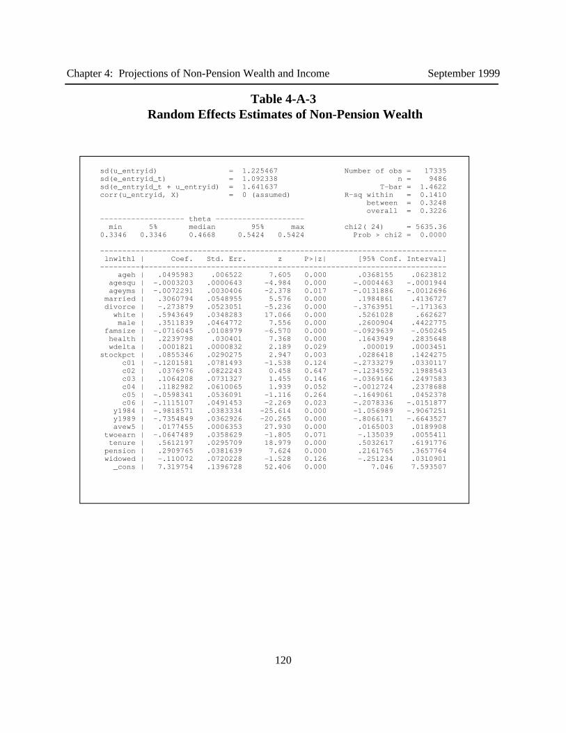
Chapter 4: Projections of Non-Pension Wealth and Income September 1999
120
Table 4-A-3 Random Effects Estimates of Non-Pension Wealth
sd(u_entryid) = 1.225467 Number of obs = 17335sd(e_entryid_t) = 1.092338 n = 9486sd(e_entryid_t + u_entryid) = 1.641637 T-bar = 1.4622corr(u_entryid, X) = 0 (assumed) R-sq within = 0.1410 between = 0.3248 overall = 0.3226------------------- theta -------------------- min 5% median 95% max chi2( 24) = 5635.360.3346 0.3346 0.4668 0.5424 0.5424 Prob > chi2 = 0.0000
------------------------------------------------------------------------------ lnwlth1 | Coef. Std. Err. z P>|z| [95% Conf. Interval]---------+-------------------------------------------------------------------- ageh | .0495983 .006522 7.605 0.000 .0368155 .0623812 agesqu | -.0003203 .0000643 -4.984 0.000 -.0004463 -.0001944 ageyms | -.0072291 .0030406 -2.378 0.017 -.0131886 -.0012696 married | .3060794 .0548955 5.576 0.000 .1984861 .4136727 divorce | -.273879 .0523051 -5.236 0.000 -.3763951 -.171363 white | .5943649 .0348283 17.066 0.000 .5261028 .662627 male | .3511839 .0464772 7.556 0.000 .2600904 .4422775 famsize | -.0716045 .0108979 -6.570 0.000 -.0929639 -.050245 health | .2239798 .030401 7.368 0.000 .1643949 .2835648 wdelta | .0001821 .0000832 2.189 0.029 .000019 .0003451stockpct | .0855346 .0290275 2.947 0.003 .0286418 .1424275 c01 | -.1201581 .0781493 -1.538 0.124 -.2733279 .0330117 c02 | .0376976 .0822243 0.458 0.647 -.1234592 .1988543 c03 | .1064208 .0731327 1.455 0.146 -.0369166 .2497583 c04 | .1182982 .0610065 1.939 0.052 -.0012724 .2378688 c05 | -.0598341 .0536091 -1.116 0.264 -.1649061 .0452378 c06 | -.1115107 .0491453 -2.269 0.023 -.2078336 -.0151877 y1984 | -.9818571 .0383334 -25.614 0.000 -1.056989 -.9067251 y1989 | -.7354849 .0362926 -20.265 0.000 -.8066171 -.6643527 avew5 | .0177455 .0006353 27.930 0.000 .0165003 .0189908 twoearn | -.0647489 .0358629 -1.805 0.071 -.135039 .0055411 tenure | .5612197 .0295709 18.979 0.000 .5032617 .6191776 pension | .2909765 .0381639 7.624 0.000 .2161765 .3657764 widowed | -.110072 .0720228 -1.528 0.126 -.251234 .0310901 _cons | 7.319754 .1396728 52.406 0.000 7.046 7.593507

Chapter 4: Projections of Non-Pension Wealth and Income September 1999
121
Table 4-A-4TOBIT Estimates of Non-Pension Wealth
Tobit Estimates Number of obs = 22657 chi2(24) =8064.97 Prob > chi2 = 0.0000Log Likelihood = -56559.635 Pseudo R2 = 0.0666
------------------------------------------------------------------------------ lnwlth1 | Coef. Std. Err. t P>|t| [95% Conf. Interval]---------+-------------------------------------------------------------------- ageh | -.0503349 .0159612 -3.154 0.002 -.08162 -.0190497 agesqu | .0007053 .0001584 4.453 0.000 .0003948 .0010157 ageyms | .0152987 .0093019 1.645 0.100 -.0029337 .033531 married | 1.515099 .131916 11.485 0.000 1.256535 1.773664 divorce | .700743 .1126127 6.223 0.000 .4800144 .9214717 white | 2.243521 .0871913 25.731 0.000 2.07262 2.414422 male | 1.291132 .0995466 12.970 0.000 1.096014 1.48625 famsize | -.2712382 .0263218 -10.305 0.000 -.3228307 -.2196457 health | .8901867 .0853516 10.430 0.000 .7228917 1.057482 wdelta | .0005052 .0002812 1.797 0.072 -.0000459 .0010564stockpct | .9972555 .0919571 10.845 0.000 .8170133 1.177498 c01 | -.0017042 .1602294 -0.011 0.992 -.3157648 .3123565 c02 | .0982653 .1685484 0.583 0.560 -.2321011 .4286318 c03 | .4778047 .1553428 3.076 0.002 .1733222 .7822871 c04 | .3200034 .1316745 2.430 0.015 .0619124 .5780943 c05 | .0210909 .1128943 0.187 0.852 -.2001896 .2423714 c06 | .0371084 .1023157 0.363 0.717 -.1634374 .2376542 y1984 | -1.706617 .1023238 -16.679 0.000 -1.907178 -1.506055 y1989 | -1.771994 .0997258 -17.769 0.000 -1.967464 -1.576525 avew5 | .0438894 .0016842 26.059 0.000 .0405882 .0471906 twoearn | .0210249 .0981525 0.214 0.830 -.1713607 .2134105 tenure | 2.527377 .0752069 33.606 0.000 2.379967 2.674788 pension | .8647954 .1055722 8.192 0.000 .6578667 1.071724 widowed | .9110909 .1559956 5.840 0.000 .6053288 1.216853 _cons | 3.746167 .3381798 11.077 0.000 3.083311 4.409023---------+-------------------------------------------------------------------- _se | 4.57969 .0264857 (Ancillary parameter)

Chapter 4: Projections of Non-Pension Wealth and Income September 1999
122
APPENDIX B ALTERNATIVE SPECIFICATION OF AGE EFFECTS
In order to capture life-cycle effects of saving and wealth accumulation, we includedvariables in our regression equation to represent the age of the family head and age-squared. Thesquared term was added to capture the fact that wealth should, at some point in the life-cycle,turn downward as households begin to dissave in retirement. Our parameter estimates had theappropriate signs -- a positive coefficient on age and a negative coefficient on age-squared. Bothwere statistically significant at a 95 percent confidence level.
Our estimates of the (mean) age-wealth profile implicit in the parameter estimates suggest,however, that the ages at which housing and other wealth begins to decline is quite high -- about81 years for housing wealth and 92 for other wealth. This means that, all other things equal, noone decumulates wealth until very late in life, a situation not observed in the cross-sectional dataon the distribution of wealth by age. Our projections do show wealth declining earlier than the agecoefficients themselves imply because the equations include an earnings term that causes wealth tobe lower as earnings decline in the latter part of the average earner’s working life.
In order to test the sensitivity of the estimates to the specification of age, we re-estimatedthe equations for housing and other wealth and substituted dummy variables for age in place ofage and age-squared. The results of these new equations are shown in Tables B-1 and B-2below. We included 11 dummy variables to capture these age effects. AGE01 was set equal toone if the family head was under 31 years of age (this variable was dropped from the estimation)and zero otherwise. AGE02 through AGE10 were set equal to one if the family head was,respectively, between 31 and 35, 36 and 40, 41 and 45, and so forth up to ages 71 and 75.AGE11 was set to one if the family head was older than 75. We also included interaction terms tocapture the effects of age and earnings. These variables are labeled AE01-AE11.
The use of dummy variables in place of the quadratic functional form does not appear tohave a significant effect on the partial relationship between age and wealth, with all other variablesconstant. We compared the two functional forms by calculating for each equation the percentagechange in non-housing wealth between ages 45 and 65, with all other explanatory variables fixed. With the quadratic form, wealth at age 65 is 51.28 percent higher than wealth at age 45. Using aseries of age dummies, as in the equations in this appendix, the change in wealth between ages 45and 65 is 51.34%, or virtually the same as with the quadratic functional form.

Chapter 4: Projections of Non-Pension Wealth and Income September 1999
123
Table 4-B-1 Projection Equation for Housing Wealth With Dummy Variables for Age
Random-effects GLS regressionsd(u_entryid) = .846745 Number of obs = 11730sd(e_entryid_t) = .6142938 n = 6324sd(e_entryid_t + u_entryid) = 1.046104 T-bar = 1.47918
corr(u_entryid, X) = 0 (assumed) R-sq within = 0.1786 between = 0.2058 overall = 0.2247------------------- theta -------------------- min 5% median 95% max chi2( 35) = 2805.390.4128 0.4128 0.5436 0.6137 0.6137 Prob > chi2 = 0.0000
------------------------------------------------------------------------------ lnhomeq | Coef. Std. Err. z P>|z| [95% Conf. Interval]---------+-------------------------------------------------------------------- ageyms | -.0004017 .0019918 -0.202 0.840 -.0043057 .0035022 married | -.0470029 .0527931 -0.890 0.373 -.1504755 .0564697 divorce | -.211301 .0529906 -3.988 0.000 -.3151607 -.1074413 white | .2524143 .0269492 9.366 0.000 .1995948 .3052337 male | .0805786 .04184 1.926 0.054 -.0014262 .1625835 famsize | .030349 .0083549 3.632 0.000 .0139737 .0467244 age02 | .3656104 .05828 6.273 0.000 .2513837 .4798371 age03 | .6702154 .0585753 11.442 0.000 .55541 .7850208 age04 | .7799013 .0613748 12.707 0.000 .659609 .9001937 age05 | .9206856 .0649748 14.170 0.000 .7933374 1.048034 age06 | 1.133275 .0658443 17.211 0.000 1.004223 1.262328 age07 | 1.204261 .0653608 18.425 0.000 1.076156 1.332366 age08 | 1.264167 .0636573 19.859 0.000 1.139401 1.388933 age09 | 1.427201 .0629528 22.671 0.000 1.303816 1.550586 age10 | 1.341704 .0657857 20.395 0.000 1.212766 1.470641 age11 | 1.394973 .0679068 20.542 0.000 1.261879 1.528068 ae02 | -.0037812 .0366009 -0.103 0.918 -.0755177 .0679553 ae03 | -.0757764 .0359853 -2.106 0.035 -.1463062 -.0052465 ae04 | -.0323214 .03655 -0.884 0.377 -.103958 .0393153 ae05 | -.0361541 .0381466 -0.948 0.343 -.1109201 .038612 ae06 | -.0793206 .0401837 -1.974 0.048 -.1580791 -.0005621 ae07 | -.0294227 .0416848 -0.706 0.480 -.1111234 .052278 ae08 | -.0074866 .0424819 -0.176 0.860 -.0907495 .0757763 ae09 | -.1540036 .053162 -2.897 0.004 -.2581991 -.0498081 ae10 | -.0499875 .1014364 -0.493 0.622 -.2487993 .1488242 ae11 | -.0942115 .1664143 -0.566 0.571 -.4203776 .2319545 health | .1104692 .021613 5.111 0.000 .0681086 .1528298 wdelta | .0954425 .0140088 6.813 0.000 .0679858 .1228993stockpct | .0708702 .0164786 4.301 0.000 .0385728 .1031676 y1984 | -.4759873 .0288525 -16.497 0.000 -.5325371 -.4194375 y1989 | -.3509022 .0268493 -13.069 0.000 -.4035258 -.2982785 avew5 | .2578843 .0321052 8.032 0.000 .1949593 .3208093 twoearn | -.0900857 .0262903 -3.427 0.001 -.1416138 -.0385577 pension | .2130511 .0256052 8.321 0.000 .1628659 .2632363 widowed | -.1118281 .0597046 -1.873 0.061 -.228847 .0051907 _cons | -.8272929 .0640202 -12.922 0.000 -.9527702 -.7018156------------------------------------------------------------------------------

Chapter 4: Projections of Non-Pension Wealth and Income September 1999
124
Table 4-B-2 Projection Equation for Other Wealth with Dummy Variables for Age
Random-effects GLS regressionsd(u_entryid) = 1.205792 Number of obs = 17335sd(e_entryid_t) = 1.093757 n = 9486sd(e_entryid_t + u_entryid) = 1.627956 T-bar = 1.4622
corr(u_entryid, X) = 0 (assumed) R-sq within = 0.1418 between = 0.3388 overall = 0.3277------------------- theta -------------------- min 5% median 95% max chi2( 36) = 5902.540.3281 0.3281 0.4601 0.5361 0.5361 Prob > chi2 = 0.0000
------------------------------------------------------------------------------lnvwlth1 | Coef. Std. Err. z P>|z| [95% Conf. Interval]---------+-------------------------------------------------------------------- ageyms | -.009167 .0031227 -2.936 0.003 -.0152874 -.0030465 married | .2289664 .0549988 4.163 0.000 .1211708 .3367621 divorce | -.2686803 .0518607 -5.181 0.000 -.3703254 -.1670353 white | .5603245 .0347573 16.121 0.000 .4922014 .6284476 male | .305683 .0462173 6.614 0.000 .2150988 .3962671 famsize | -.0553805 .0110676 -5.004 0.000 -.0770725 -.0336885 age02 | .2189216 .061184 3.578 0.000 .0990032 .3388399 age03 | .4133094 .0669148 6.177 0.000 .2821587 .5444601 age04 | .5876249 .0738286 7.959 0.000 .4429234 .7323264 age05 | .7478025 .082601 9.053 0.000 .5859075 .9096975 age06 | .6679172 .0865916 7.713 0.000 .4982008 .8376336 age07 | .9032182 .0863747 10.457 0.000 .7339269 1.072509 age08 | 1.002014 .0829289 12.083 0.000 .8394768 1.164552 age09 | 1.127883 .0803806 14.032 0.000 .9703399 1.285426 age10 | 1.140505 .0837755 13.614 0.000 .9763084 1.304702 age11 | 1.222803 .0850703 14.374 0.000 1.056068 1.389538 ae02 | -.0080804 .0430363 -0.188 0.851 -.09243 .0762691 ae03 | -.0260821 .0435074 -0.599 0.549 -.111355 .0591908 ae04 | -.0373977 .045359 -0.824 0.410 -.1262998 .0515044 ae05 | -.008029 .0489515 -0.164 0.870 -.1039722 .0879142 ae06 | .0357198 .0535514 0.667 0.505 -.069239 .1406785 ae07 | .0076826 .0570606 0.135 0.893 -.104154 .1195193 ae08 | -.0557424 .0592061 -0.941 0.346 -.1717843 .0602994 ae09 | .1495142 .0798942 1.871 0.061 -.0070755 .3061039 ae10 | .0050059 .1588551 0.032 0.975 -.3063444 .3163563 ae11 | .1215177 .2578508 0.471 0.637 -.3838605 .626896 health | .1789965 .0301379 5.939 0.000 .1199274 .2380656 wdelta | .348186 .0205226 16.966 0.000 .3079625 .3884095stockpct | .0783248 .0289695 2.704 0.007 .0215456 .1351041 y1984 | -.917398 .0387157 -23.696 0.000 -.9932795 -.8415165 y1989 | -.7235808 .0364028 -19.877 0.000 -.7949289 -.6522326 avew5 | .5957117 .0365947 16.279 0.000 .5239873 .667436 twoearn | -.1125771 .037173 -3.028 0.002 -.1854349 -.0397193 tenure | .5313395 .0295915 17.956 0.000 .4733413 .5893376 pension | .3932966 .0391116 10.056 0.000 .3166393 .4699539 widowed | -.163029 .0719575 -2.266 0.023 -.3040631 -.0219949 _cons | -1.975892 .0584115 -33.827 0.000 -2.090377 -1.861408------------------------------------------------------------------------------
Chapter 4: Projections of Non-Pension Wealth and Income September 1999
125
CHAPTER 4: REFERENCES
Gustman, A. L. and F. T. Juster (1996), “Income and Wealth of Older American Households:Modeling Issues for Public Policy Analysis”, ”, in Hanushek, E. A. and N. L. Maritato,Editors, Assessing Knowledge of Retirement Behavior, Committee on National Statistics,National Research Council.
Hurd, M. D. (1990), “Research on the Elderly: Economic Status, Retirement and Consumptionand Saving”, Journal of Economic Literature, June, 28(2), pp. 565-637.
Modigliani, F. and R. Brumberg (1954), “Utility Analysis and the Consumption Function: AnInterpretation of Cross-Section Data”, in Kurihara, K.K. (ed.), Post-KeynesianEconomics, Rutgers University Press, New Brunswick, NJ.
CHAPTER 4: LIST OF TABLES
Table 4-1Comparison of SIPP and PSID Family Wealth Data: Mean Housing Wealth Divided by Economy-Wide Average Wage, by Age 94
Table 4-2Comparison of SIPP and PSID Family Wealth Data: Mean Other, Non-Pension Wealth Divided by Economy-Wide Average Wage, by Age 95
Table 4-3Comparison of Family Wealth on the SIPP with the PSID at Fixed Percentiles of the Wealth Distribution (in 1996 Dollars) 96
Table 4-4Random Effects Model for Home Ownership 101
Table 4-5Random Effects Model for Home Equity 102
Table 4-6Random Effects Probit Model for Presence of Positive Other Wealth 103
Table 4-7Random Effects Model For Other Wealth 104
Table 4-8Mean Values of Selected Independent Variables at Age 62, By Birth Cohort 106
Table 4-9Mean Housing Wealth as a Fraction of the Economy-Wide AverageWage at Ages 62 and 67, by Birth Cohort — All Individuals 108

Chapter 4: Projections of Non-Pension Wealth and Income September 1999
126
Table 4-10Mean Housing Wealth as a Fraction of the Economy-Wide AverageWage at Ages 62 and 67, by Birth Cohort — Married Individuals 108
Table 4-11 Mean Housing Wealth as a Fraction of the Economy-Wide AverageWage at Age 62, by Birth Cohort — Single Individuals 108
Table 4-12Mean Housing Wealth as a Fraction of the Economy-Wide Average Wage at age 62, byBirth Cohort and Income Quintile - All Individuals 110
Table 4-13Mean Housing Wealth as a Fraction of the Economy-Wide Average Wage at age 67, by Birth Cohort and Income Quintile - All Individuals 110
Table 4-14 Mean Other Wealth as a Fraction of the Economy-Wide Average Wage at Ages 62 and 67, by Birth Cohort — All Individuals 112
Table 4-15 Mean Other Wealth as a Fraction of the Economy-Wide Average Wage at Ages 62 and 67, by Birth Cohort — Married Individuals 112
Table 4-16 Mean Other Wealth as a Fraction of the Economy-Wide Average Wage at Ages 62 and 67, by Birth Cohort — Single Individuals 112
Table 4-17Mean Other Wealth as a Fraction of the Economy-Wide Average Wage at Age 62, by Birth Cohort and Income Quintile - All Individuals 113
Table 4-18Mean Other Wealth as a Fraction of the Economy-Wide Average Wage at age 67, by Birth Cohort and Income Quintile - All Individuals 113
Table 4-19Coefficient of Variation of Wealth Estimates, By Birth Cohort 115
Table 4-A-1OLS Estimates of Non-Pension Wealth 118
Table 4-A-2 Median Regression Estimates of Non-Pension Wealth 119
Table 4-A-3 Random Effects Estimates of Non-Pension Wealth 120
Table 4-A-4TOBIT Estimates of Non-Pension Wealth 121
Table 4-B-1 Projection Equation for Housing Wealth With Dummy Variables for Age 123
Table 4-B-2 Projection Equation for Other Wealth with Dummy Variables for Age 124

Chapter 4: Projections of Non-Pension Wealth and Income September 1999
127
1. This differs slightly from the way cohorts are defined in other tables presented in this report,where the first cohort begins in 1931.
2. Including age, time and cohort effects results in an equation that is over-determined since, bydefinition, t = a + c where t equals time, a equals age and c is cohort (year of birth). Perfectcollinearity was not present in the estimated model because the cohort dummies were defined inbroad, 5-year age groups. Nevertheless, the estimates of the cohort effects need to be interpretedwith caution.
3. For a small number of families with negative wealth, we set these values to zero.
4. This seems like a reasonable assumption to make for housing wealth. That is, it is unlikelythat someone who did not own a home at age 62 would purchase one by age 67. This assumptionhad very little effect on the results.
CHAPTER 4: ENDNOTES

128
CHAPTER 5
PROJECTIONS OF RETIREMENT DECISION
I. OVERVIEW
For nearly eight percent of the MINT sample, administrative data provide information ontiming of first receipt of old-age and survivor benefits from Social Security.1 For the remainder ofthe MINT population, a statistical model assigns timing of Social Security benefit receipt. Thismodel combines both stochastic (equation-based) and deterministic (rule-based) functions. Thedeterministic functions mandate benefit receipt for low-earning widows and widowers who arewidowed at or before age 60 or 61.2 For those in the population who are not low-earningwidowers thus defined, logistic equations determine each individual’s probability of receivingSocial Security at each age t between 62 and 67 given that he/she did not receive benefits at age t-1. The logistic equations are reduced-form rather than structural in nature. That is, instead ofdirectly relying on rules about optimizing behavior near retirement, they capture the existingrelationship between an individual’s benefit receipt timing and aspects of his/her life trajectory(e.g., educational, marital, and earnings history) and fixed characteristics (e.g., sex).3 Theequations were estimated from Survey of Income and Program Participation (SIPP) data matchedto Summary Earnings Records (SER) and the Social Security Administration’s Master BeneficiaryRecord (MBR). The SIPP panels used for estimation included 1990 through 1993.
II. TIMING OF RECEIPT OF SOCIAL SECURITY RETIREMENTBENEFITS
1. Estimation Strategy
We estimated separate logistic equations for three groups--married males, marriedfemales, and unmarried males and unmarried females pooled together.4 We screened individualsin the sample for receipt of Social Security disabled worker benefits based on the payment datesthat the Master Beneficiary file reports, and excluded any individuals who had, to date, receiveddisabled worker benefits from the population. Such cases made up just over five percent of thetotal number of person-year observations. Sample sizes for nondisabled members of the threefinal estimation groups were as follows: 2,808 person years at risk for currently married men;2,283 person years at risk for currently married women; and 2,147 person years at risk for menand women who were not currently married.
To estimate the equations, we examined SIPP participants late in the year of each singleyear of age from age 62 onward to see if they had, according to MBR data, begun to receiveSocial Security benefits in that year.5 Figure 5-1, based on SIPP and MBR data, shows patterns

Chapter 5: Projections of Retirement Decision September 1999
129
-500
1500
3500
5500
7500
0 12 24 36 48 60 72 84 96 108
120
132
Months beyond age 60
Fre
quen
cy
MBR
SIPP
Figure 5-1 Month of First Benefit Entitlement,
Where First Entitlement is Age 60 or Above, Using SIPP and MBR Birthdates
Source: Urban Institute tabulation from 1990-1993 SIPP matched to the 1990-1993 MBR (462cases unmatched)Sample: Individuals who, according to SIPP birthdate, reach any age between 61 and 70 at anypoint during the life of the panelMBR N=26,867 (7,768 cases missing, 283 cases with invalid dates of first receipt, 2,827 earlyrecipients)SIPP N=24,040 (10,221 cases missing, 0 cases with invalid dates of first receipt, 3,946 earlyrecipients)

Chapter 5: Projections of Retirement Decision September 1999
130
of Social Security receipt for persons in the estimation data. The figure reveals that SocialSecurity benefit receipt is highly clustered around one’s birth date at ages 62 (24 months beyondage 60) and 65 (60 months beyond age 60). (The figure also illustrates an important measurementissue that both endnote one and Appendix A discuss.) Because the unit of analysis is a person-year, a single person could be represented in the estimation file more than once (to a maximum offour times, in the 1991 panel which tracked some households for up to 40 months). About 88percent of the person-year observations from SIPP were matched to an earnings record. Thoseobservations for which a match was not obtained were then dropped from the sample. Alsoexcluded were those individuals who took up their Social Security benefits at age 60 or 61, giventhat they are, as described above, excluded from the stochastic determination process.
To replicate the actual benefit application process as closely as possible, we attempted toscreen the sample for eligibility for Social Security retirement benefits, based on SER informationon both one’s own and one’s current spouse’s OASDI coverage history and any other evidence ofSocial Security benefit eligibility. We abandoned this effort for three reasons. First, exactlydefining the Social Security-eligible population based on the SIPP-match files was not possible,because not all former spouses of members of the sample can be observed. Second, the crudeeligibility screen greatly diminished sample sizes. Third, eliminating the screen did not causemajor changes to parameter estimates.6
Most determinants in the descriptive prediction equations are contemporaneous, althoughin some cases we used lagged values. Explanatory variables within each group include age (codedas single-year dummies), education (coded categorically), and measures of earnings, income, andwealth, all of which are expressed in relation to the average national wage. Earnings measuresinclude covered earnings at year t-1,7 average covered earnings in younger working years (ages35 to 55), and recent covered earnings (from ages 56 to 61). Whether one is covered by either adefined benefit (DB) pension or a defined contribution (DC) retirement account (e.g., an IRA,Keogh, or 401(k) plan) is another determinant in the equations.8 Other wealth measures in themodel include family net worth less home value and home equity, sometimes coded as a dummyvariable indicating whether this is greater than zero and other times the actual value. Preliminaryestimates considered asset income, but the direct wealth measures just described are moreconsistent with the estimates in Chapter Four. An indicator of race-ethnicity, specifically adummy variable for non-Hispanic whites versus others, is also included in the models.
For individuals who were married in the month of potential Social Security receipt,additional variables in the logistic equations describe the spouse’s characteristics, including his/herage, earnings history, education, and wealth, including pension coverage. The spouses ofmembers of the estimation sample were born as early as 1908 and as late as 1970. As a result, aspouse’s earnings could always be examined at t-1, but information was not always available onher/his average earnings from the ages 35 to 55. Where spouses were too old to have reportedearnings from this age range, we used their earnings from the years 1951 to 1971 as a proxy. Where spouses were too young, we took their 20 most recent years of earnings (through 1996).

Chapter 5: Projections of Retirement Decision September 1999
131
Preliminary regressions suggested that several additional variables are good predictors ofthe timing of receipt of Social Security benefits. These include the duration of one’s most recentwork spell (i.e., how long it has been since one had a zero earnings year) and one’s total numberof years in the labor force, both of which can be considered measures of attachment to the laborforce and perhaps “taste” for work. We have not included these in the current MINT modelbecause the approach for forecasting earnings trajectories in MINT that Chapter Two describes,while effective at generating AIMEs, is not particularly effective at generating realistic patterns ofspells of work/not work in employment histories. This choice may be worthy of re-considerationat some future point in MINT’s development.
2. Coefficient Estimates
Table 5-1 reports the logistic estimates for the final models for the three separate groups,including the standard errors and significance levels for each coefficient. Coefficients from theequations can be interpreted as the effects of each variable on the log-odds of taking up SocialSecurity benefits at age t given non-receipt at age t-1.
The results in Table 5-1 suggest that across all three of these groups, age, earnings, andrace-ethnicity are consistently strong predictors of timing of Social Security benefit receipt. Agehas non-linear effects on the probability of receipt, with individuals generally more likely to retireat ages 62 and 65 than at 63, 64, and older ages, all else being equal. Both social norms andincentives (e.g., eligibility for Medicare at age 65) contribute to this pattern. While earningsbetween ages 35 and 55 and between ages 56 and 61 are both positively associated with thelikelihood of benefit receipt (i.e., the higher the average earnings, the greater the likelihood ofcollecting Social Security) for nearly all groups, earnings at t-1 are negatively associated withreceipt. This pattern is sensible, since those with higher lifetime earnings have greater resourcesfrom which to draw, making a comfortable retirement more likely, yet those continuing to workbeyond age sixty both demonstrate higher current earning ability and have already exhibited thatthey are less likely to retire for some unobservable reason (perhaps a “taste” for work, asdescribed above). For all three groups, those persons who are non-Hispanic whites begin benefitreceipt at a significantly faster rate than those who are not (i.e., Hispanic whites and nonwhites),other factors being equal.
In these estimates, whether one is covered by a pension has differing effects on SocialSecurity benefit take-up across the groups. Pensions represent resources from which a person candraw in retirement, but they also might suggest characteristics of one’s employer. While pensioncoverage serves to accelerate married men’s retirement timing, it serves to decelerate marriedwomen’s retirement timing. For married women, a spouse’s pension coverage, does, however,increase the probability of starting Social Security receipt, though not significantly. For singlepeople, pension coverage does has a positive coefficient (implying that coverage makes SocialSecurity retirement more likely), though the relationship with benefit take-up is not statisticallysignificant at the .05 level.

Chapter 5: Projections of Retirement Decision September 1999
132
Table 5-1Logistic Regression Coefficients Currently Employed in MINT:
Social Security Benefit Receipt Timing
Parameter Estimate (Standard Error)
Variable Married Men(N=2808)
Married Women(N=2283)
Unmarried People(N=2147)
Intercept -2.3859** (0.5465) -2.2842** (0.7561) -0.5755** (0.1601)
Age 63 -1.1243** (0.1304) -1.6080** (0.1448) -1.3359** (0.1456)
Age 64 0.3890** (0.1235) -0.5367** (0.1418) -0.4756** (0.1322)
Age 65 1.4978** (0.1621) -0.1443 (0.1763) 0.5582** (0.1508)
Age 66 -0.2732 (0.2488) -1.2332** (0.2456) -1.1512** (0.2243)
Age 67 -0.8792** (0.3017) -1.2641** (0.2532) -0.5951** (0.1961)
Education < 12 0.1340 (0.1250) -0.1014 (0.1349) 0.2210 (0.1227)
Education > 12 -0.1702 (0.1174) -0.0927 (0.1251) -0.1775 (0.1201)
Non-Hispanic white 0.4141** (0.1491) 0.3157* (0.1473) 0.4088** (0.1180)
Have any pension? 0.3292** (0.1067) -0.3119** (0.1109) 0.0299 (0.1087)
Earnings ages 35-55 1.6485** (0.1455) 1.4474** (0.2427) 0.9120** (0.1728)
Earnings ages 56-61 0.3440** (0.1277) 0.2942 (0.2464) 0.0851 (0.1736)
Earnings at t-1 -1.4664** (0.1004) -1.7848** (0.2207) -0.7840** (0.1380)
Spouse’s age 0.0133 (0.00869) 0.0289** (0.0112)
Spouse’s education < 12 0.1104 (0.1255) 0.1953 (0.1379)
Spouse’s education > 12 -0.1012 (0.1162) -0.1495 (0.1285)
Spouse’s earnings 35-55 0.3421* (0.1534) 1.0697** (0.1061)
Spouse’s earnings at t-1 -0.1654 (0.1121) -0.5266** (0.0703)
Spouse has a pension? 0.1381 (0.1149)
Male -0.1172 (0.1143)
Widowed 0.1542 (0.1015)
Log value of non-housing wealth -0.0155 (0.0524)
Own a home -0.0441 (0.1042)
Value of home -0.0257 (0.0148)
* indicates p<.05; ** indicates p<.01

Chapter 5: Projections of Retirement Decision September 1999
133
Once earnings and pensions are taken into account, education has little to no effect on thetiming of Social Security benefit receipt. Married men and single persons with less than a highschool education are more likely to start Social Security retirement than are their counterpartswith a high school degree (the omitted category), and more educated persons in all three groups,those with greater than a high school education, are less likely to begin receipt than their less well-educated colleagues. However, none of these relationships is statistically significant. If thecoefficients were significant, such patterns would not be surprising, as education is likely to behighly correlated with the prospect of having a rewarding job. For married women in thesecohorts, however, there is a somewhat different relationship between education and benefitreceipt timing. For them, the less-educated are less likely than the high school graduates to retire,though again we cannot say with any confidence that this coefficient differs from zero. Asmarried women’s educational and earnings trajectories begin to resemble married men’s moreclosely, the factors influencing women’s decisions about Social Security may change. This caseillustrates the general difficulties that one faces using estimates from data on current workers intheir sixties to project patterns for workers who will enter their sixties in the next century.9
A spouse’s mid-career earnings (again, measured from age 35 to 55, with exceptionsnoted above) appear to have a significant, positive influence on the likelihood of benefit receipt ofboth married men and married women in these cohorts. A spouse’s lagged earnings are also quiteimportant for both husbands’ and wives’ benefit timing, negatively associated with receipt (thoughthe coefficient is not significant for the married men). Among both married men and marriedwomen, a spouse’s age appears to play a minor role in this process: the older one’s spouse, themore likely a person is to begin receiving benefits, though this coefficient was not statisticallysignificant for the married men. A spouse’s education does not have significant effects on marriedpersons’ Social Security take-up net of these other factors, though the signs mirrored the effectsfor a person’s own education (the likelihood of receipt decreases with more education).
We found that measures of family wealth had negligible effects on the timing of SocialSecurity benefit receipt once all these other elements were taken into account.10 Likewise,housing wealth had only marginally significant effects. Overall, individuals’ earnings and,implicitly, the Social Security wealth that they generate thus appear far more important to thisprocess than other forms of wealth.
3. Simulation of Eligibility Screen
These three equations were applied to a subset of the MINT population that was screenedfor OASDI eligibility, based upon the individual’s and, where applicable, his/her spouse’s quartersof Social Security coverage. To screen for eligibility, we compute a Primary Insurance Amount(PIA) for each person in the sample. If the PIA is above zero, then he or she is eligible to retire inhis/her own right. We also check, where applicable, each person’s current or past SocialSecurity-qualified spouse or spouses. If a person is not currently married (or was widowed butremarried after age 60) and he or she has had more than one Social Security qualifying marriage,

Chapter 5: Projections of Retirement Decision September 1999
134
we examine multiple past spouses for a non-zero PIA that would render the person qualified forbenefits.
4. Assignment of Retirement Timing with Scheduled Increases in the NormalRetirement Age
As these equations were estimated on recent SIPP data, they depict patterns of SocialSecurity benefit timing under the current Social Security system, in which the Normal RetirementAge is set at 65 and the Age of Earliest Eligibility is set at 62. For the sake of simplicity andcloser integration with other aspects of the model, in the projections we assume that workers electto receive their benefits by or at the ultimate Normal Retirement Age (67). Although this hasclearly never been the case historically, it is true that only a small fraction of past workers, aroundsix percent in recent years, have elected to receive their benefits after the Normal Retirement Age. Model users might consider extending the sample to include people at risk up to age seventy, thepoint at which the benefit of delaying benefit receipt falls to zero. We have re-estimated theequations to include more people (i.e., those who still have not applied for Social Securitybenefits at ages 67 through 69), thus allowing MINT users to relax the assumption of universalreceipt by age 67 in future work. Table 5-A-3 in the appendix presents sample estimates oflogistic coefficients where the age of first receipt is not capped at 67, but rather at age 69.
Some of the birth cohorts of greatest interest for MINT will begin to receive SocialSecurity benefits after 1999, and will thus face a Normal Retirement Age that will be higher thanage 65 but an Age of Earliest Eligibility that will be set at the same level as today (62). (Table 7-A-1 in Chapter Seven depicts the scheduled increases in the Normal Retirement Age, by birthcohort.) Applying the SIPP equations to populations that will face a different set of SocialSecurity rules is surely problematic. Unfortunately, we cannot directly estimate the effects of theNormal Retirement Age (or changes to the NRA) on retirement benefit receipt timing patternsbecause it has not varied in the years for which we have reliable data.11 We must therefore insteadmake assumptions, ideally guided by theory and empirical research, about whether changes inretirement behavior will accompany this change in policy and, if so, how large these changeswould be. While we have made the implicit assumption that changes will be negligible, there areseveral ways that we could modify this assumption.
A first way to modify this assumption would be simply to adjust the coefficients on the ageterms in the projection in an ad hoc fashion to achieve a targeted level of behavioral adjustment. One could, for example, use estimates of behavioral response from the Social Security Office ofthe Chief Actuary to set these targets.
Using expected Social Security benefits or Primary Insurance Amounts rather than lifetimeearnings as explanatory variables in these equations is another feasible, and perhaps moresatisfying but nonetheless still ad hoc, way to extend the model and modify this assumption.12 Such an approach would both capture the non-linear replacement of income by Social Security

Chapter 5: Projections of Retirement Decision September 1999
135
and also allow us to account explicitly for changes in future Social Security benefits alreadymandated in the law through the increases in the Normal Retirement Age. In changing the modelin this way, we would need to be cautious and to consider that individuals’ responses to benefitchanges may not mirror the existing variation in receipt choices by benefit levels. Responses tochanges in benefits might also be better captured using benefit thresholds rather than continuousbenefit levels (which would imply that individuals always shift with a benefit cut) or perhapsinteractions between benefit and educational levels.
In other work, several members of the Urban Institute MINT team have used these samedata (SIPP matched to the MBR and SER) to attempt to estimate the effects of tax rates onearnings on work and benefit receipt choices (See Favreault, Ratcliffe, and Toder, 1999). Theydeveloped a joint model of Social Security benefit receipt and work (at and after age 62). Ratherthan applying the MINT Chapter Five and Chapter Six functions sequentially, in this work, asingle, multinomial hazard model predicts individuals’ transitions into one of four separate states:collect Social Security benefits and not work, collect Social Security benefits and work, do notcollect Social Security benefits and work, do not collect Social Security benefits and do not work. Such a model implies that work and benefit receipt choices are so tightly coupled that one bestrepresents them with a single process. Predictors in this model included one’s expected SocialSecurity benefit at the time of potential receipt, which had a negative effect on the likelihood ofworking (i.e., the higher the benefits, the less likely it is that one would work), and the total taxrate on earnings, which also had a negative effect on work effort (i.e., the higher the tax rate onearnings, the less likely it is that one would work). Researchers at SSA may wish to considerimplementing this sort of specification in MINT. As with the current, binary model, one needs tobe cautious about interpreting the results of such a reduced-form model in the face of structuralchanges to Social Security. The model can nonetheless give some limited insight into thepotential directions and magnitudes of benefit receipt and work choices in the face of scheduledbenefit cuts (e.g., by means of the increase in the Normal Retirement Age).
While Figure 5-1 reveals that individuals’ dates of first receipt cluster around their birthmonth at ages 62 and 65, it also suggests that they do not cluster in this way at ages 63 and 64. Further, into the future, individuals may be influenced by the Normal Retirement Age signal ofage 65 or 66 and a certain number of months. Accounting for heterogeneity in Social Securitybenefit timing within single-year age groups could thus be advantageous for investigating changesthat would result from raising the Early and/or Normal Retirement Ages. The model describedhere could be extended to account for within-year heterogeneity in several different ways. Wehave chosen the simplest approach: imposing within-year heterogeneity randomly by usinghistorical distributions. This approach should be adequate unless there are significantdistributional differences in within-year benefit timing (e.g., if it is the case that wealthy people aremore likely to retire right after a birthday, while less well-off people are more likely to apply forbenefits mid-year).
If this assumption of randomly distributed within-year variation in retirement timing isproblematic, these differentials could be integrated into the model in the estimation phase.

Chapter 5: Projections of Retirement Decision September 1999
136
Maintaining a discrete-time event history framework, we could examine semi-annual, quarterly, oreven monthly observations on the persons at risk, rather than annual ones.13 We couldalternatively model the dependent variable as a continuous rather than discrete outcome andestimate a continuous-time hazard model, since exact dates of birth and months of Social Securityreceipt are available in the estimation data sources. Continuous- and discrete-time event historymodels tend to yield similar results (see, for example, discussion in Alison, 1984), but havedifferent limitations and requirements.
5. Results from Simulation Analyses
When we use these estimated coefficients from SIPP to project timing of Social Securitybenefit receipt for members of the MINT population, we find that almost 60 percent (4.6 + 1.2 +53.9) of eligible individuals elect to receive their benefits at or before age 62. Table 5-2 reportsthe frequency of retirees at each age in Column A and the corresponding weighted andunweighted percentages in Columns B and C. The table reveals that the weighted andunweighted distributions from MINT are very similar, and henceforth, we present weightedestimates.
Table 5-2Percentages of MINT and Historical (1996) Populations Electing
to Receive Social Security Benefits at Given Ages
MINT Predictions Historical Estimates Difference
Age
A B C D E F G H (C-G)
UnweightedFrequency
Unweighted Percentage
Weighted Percentage
All Retired Workers
D LessDisabilityConver-sions
E PlusWives* ofRetiredWorkers
F PlusMostSurvivors
MINT MinusMost Similar Historical
60 3,752 4.8 4.6 - - - 4.6 0
61 1,019 1.3 1.2 - - - 1.3 -0.1
62 41,980 53.4 53.9 53.1 60.1 59.5 56.5 -2.6
63 7,961 10.1 10.3 6.6 7.5 7.6 7.1 +3.2
64 11,226 14.3 14.2 9.6 10.8 10.7 9.9 +4.3
65 7,646 9.7 9.6 25.4 15.7 15.3 14.2 -4.6
66 1,654 2.1 2.0 1.8 2.0 2.1 1.9 +0.1
67+ 3,752 4.4 4.2 3.5 4.0 4.7 4.4 -0.2
N/A 34,399
*Husbands of retired workers are not included in this column because of the small number of affected cases.MINT Source: Urban Institute tabulations, September, 1999 Historical Source: Annual Statistical Supplement, 1997, Tables 6.A4 and 6.D3

Chapter 5: Projections of Retirement Decision September 1999
137
Table 5-2 also contrasts the estimates for the MINT population to similar historicalestimates based on Social Security Administration data. There are no historical data that areexactly analogous to the estimates the model produces, because people who die before receivingbenefits or who do not apply for benefits despite their eligibility are not included in Social Securityrecords. The closest source for comparison is new award data for those first receiving SocialSecurity retirement benefits in 1996 (the most recent year for which detailed statistics areavailable), from which we can construct a synthetic retirement cohort.14
For these comparisons, we first consider data on retired workers (in Column D). We needto eliminate disability conversions from these historical estimates, because individuals whoconverted their benefits from DI to retired worker benefits were not included in either the originalestimation or the projection. When we do so, in Column E, we see that the historical spike inSocial Security receipt at age 65 declines greatly, and an even higher proportion of workersretires at 62. We also wish to include spouse recipients in our comparisons, because they wereincluded in both the estimation and projection phases. We add them in Column F, causing onlyminor changes to the totals retiring at each age. Survivors whose first Social Security receipt is asa survivor should also be included in these estimates. We do so in Column G, but caution thatthis poses some challenges.15
Contrasting the MINT projection estimates (Column C) to the closest possible historicaldata on benefit receipt timing (Column G), we see some similarities. Differences between the twoestimates are presented in Column H. The proportions of Social Security recipients retiring atages 62 and 65 are somewhat lower in MINT than in the historical figures, while proportionsstarting Social Security at 63 and 64 are a bit higher in MINT than observed historically. Otherwise, though, the patterns are quite close. While the discrepancies at ages 62 and 65 maysuggest potential improvements for the model, we should of course expect some differencesbetween the MINT and historical estimates. The composition of the U.S. population eligible forSocial Security should change considerably between 1996 and 2031 (the year that the youngestmembers of the MINT sample turn age 66). Women’s greater likelihood of receiving SocialSecurity benefits as workers (as opposed to solely as wives) could be playing an especiallyimportant role in the changes. Further, the method employed for projecting earnings leads tosubstantially different distributions of the variable for earnings at time t-1, one of the keydeterminants of benefit receipt timing, in the projection and estimation samples. For men, meanson this variable are much lower in the projection sample than in the estimation group, leading tohigher predicted probabilities, and hence more retirements at ages 63 and 64, than we observehistorically. For women, we see similar, though less extreme, results at ages 63 and 64.
The final row in Table 5-2, labeled “N/A,” reveals that almost 35,000 MINT persons, justover thirty percent of the total, are not assigned a Social Security retirement age in the model. There are three reasons why an individual would not be assigned a benefit receipt age: he or shedied before becoming eligible for Social Security (and, to promote consistency with earningsprojections in Chapter 2, this includes attainment of eligibility within the year of death) or before

Chapter 5: Projections of Retirement Decision September 1999
138
electing to retire, he or she became disabled (as defined using the DI_PRED variable that is usedin Chapter 2) before retirement, or he or she is not eligible for a Social Security benefit.16 About aquarter of the MINT population dies or becomes disabled before reaching age 62, and almost athird before reaching age 67. Only a small fraction of the MINT population is ineligible for SocialSecurity as either a worker or a spouse, a total of just under 5,300 persons, or a bit less than 4.7percent of the total population. Individuals in this group include long-term government workerswho are not married to Social Security qualified workers and also individuals without significantattachment to the labor force.
Returning to those members of the MINT population designated to be Social Securityrecipients, Tables 5-3A and 5-3B document important distributional differences for men andwomen, respectively, between those who elect to receive their benefits early and those whocollect Social Security later. The differences by sex that are revealed in these tables appear to bequite important. On average, MINT women elect to receive Social Security benefits about aquarter of a year earlier than do MINT men (men’s average age at first receipt is 63.01, whilewomen’s is 62.74). About 64 percent of MINT women receive their benefits at or before age 62,compared to just over 54 percent of all men. While women tend to receive their benefits earlierthan men, they are also slightly more likely to wait until age 67 before receiving them than aremen. This projected gender differential in benefit receipt timing is similar to that observed inhistorical data. Table 5-A-4 in the Appendix details differences between the MINT and historicalestimates by sex.
Marriage patterns also appear to be quite important to benefit timing, with ever marriedwomen projected to begin benefit receipt on average almost a year earlier than their never marriedcounterparts. While 65 percent of ever married women begin to receive Social Security benefit ator by age 62, only 44 percent of the never married women do. The availability of noncontributorybenefits to ever married women surely plays an important role in this difference. Never marriedmen also retire later than ever married men, by about half a year, but the difference is not quite asextreme as with the women. This suggests that the never married men may have more resourcesfrom which to draw than do the never married women. Racial differences in benefit timing alsoappear quite sizable in these tables, with nonwhite men and women more likely to postponeretirement than white men and women. The proportion of nonwhites retiring at age 67 is aboutdouble the proportion of whites retiring at this age for both men and women. On average,nonwhites retire about a third of a year later than whites.
Patterns in benefit receipt by birth cohort are less obvious than the gender, racial, ormarital history patterns. The figures do not reveal any clear pattern in Social Security receiptacross the cohorts in MINT.17 The lack/modesty of cohort change observed in these projectionsis surely due in part to our assumption of no change in behavior with increments to the NormalRetirement Age. One can justify such an assumption by the fact that Social Security offers socompelling a change in income from non-work at age 62 that changes to benefit levels may needto be quite large to offset the lure of retirement, especially for those in unrewarding occupations. We are unsatisfied with this assumption, however, and hope to pursue alternative specifications.

Chapter 5: Projections of Retirement Decision September 1999
139
Table 5-3A Projected Percentage of MINT Men in Various Demographic and Economic
Groups Electing to Receive Social Security Benefits at Given Ages
60 61 62 63 64 65 66 67 Mean
All Men 1.0 0.3 53.1 12.1 17.3 10.7 1.8 3.6 63.01
Ever married 1.1 0.3 53.4 12.2 17.4 10.6 1.7 3.3 63.00
Never married - - 46.9 10.8 14.0 13.3 4.9 10.1 63.49
1931-35 0.3 0.1 54.4 10.9 17.8 12.3 1.0 3.2 63.02
1936-40 0.7 0.1 53.1 12.5 19.4 10.4 1.4 2.4 62.98
1941-45 0.8 0.3 55.5 13.6 16.7 8.9 1.1 3.0 62.85
1946-50 1.0 0.2 53.9 12.9 17.8 9.5 1.4 3.1 62.83
1951-55 1.3 0.4 54.6 13.4 16.5 9.5 1.3 3.1 62.98
1956-60 1.4 0.3 54.0 12.8 17.2 9.7 1.2 3.3 62.88
Nonwhite 2.0 0.7 43.1 11.8 16.8 15.4 3.0 7.2 63.34
White 0.9 0.3 54.6 12.2 17.3 10.1 1.7 3.1 62.98
1st real AIME quintile 5.1 1.1 34.6 7.7 15.2 16.7 3.4 16.1 63.70
2nd real AIME quintile 2.8 1.0 41.1 8.4 18.4 18.2 3.0 7.1 63.41
3rd real AIME quintile 1.4 0.6 49.9 11.0 19.9 12.2 1.8 3.3 63.07
4th real AIME quintile 0.3 0.1 55.0 13.9 17.6 9.7 1.7 1.7 62.93
5th real AIME quintile 0.0 0.0 60.6 13.4 16.0 7.4 1.2 1.3 62.78
Source: Urban Institute tabulation from MINT file, September, 1999

Chapter 5: Projections of Retirement Decision September 1999
140
Table 5-3BProjected Percentage of MINT Women in Various Demographic and
Economic Groups Electing to Receive Social Security Benefits at Given Ages
60 61 62 63 64 65 66 67 Mean
All Women 7.4 2.0 54.6 8.8 11.7 8.6 2.2 4.8 62.74
Ever married 8.1 3.0 54.2 9.5 11.1 8.2 1.1 4.9 62.66
Never married - - 45.0 10.5 16.7 14.0 1.1 12.7 63.55
1931-35 7.4 3.0 55.5 8.6 11.1 8.5 1.9 4.0 62.66
1936-40 8.8 2.5 55.6 7.7 11.9 7.8 1.7 4.0 62.61
1941-45 9.2 1.9 55.0 8.2 12.2 8.0 1.4 4.0 62.56
1946-50 7.3 1.6 57.7 8.7 11.8 8.2 1.3 3.4 62.63
1951-55 7.1 1.9 56.7 8.9 11.6 7.9 1.6 4.3 62.68
1956-60 6.8 1.7 55.3 9.7 12.3 8.6 1.8 3.8 62.71
Nonwhite 8.4 2.2 46.0 8.7 12.3 11.4 2.7 8.3 63.01
White 7.3 1.9 56.0 8.8 11.6 8.1 2.1 4.2 62.69
1st real AIME quintile 15.0 2.1 51.8 6.9 9.2 6.7 2.6 5.7 62.52
2nd real AIME quintile 9.4 3.4 53.3 8.4 11.1 8.6 1.6 4.2 62.62
3rd real AIME quintile 2.3 1.8 56.4 9.8 13.1 9.6 2.3 4.9 62.92
4th real AIME quintile 0.7 0.6 56.7 10.7 14.5 10.4 2.3 4.1 62.99
5th real AIME quintile 0.2 0.1 59.5 10.6 13.6 9.9 1.9 4.2 62.96
Source: Urban Institute tabulation from MINT file, September, 1999

Chapter 5: Projections of Retirement Decision September 1999
141
Position in the income distribution, defined by ranking people by unisex quintiles ofaverage indexed monthly (covered) earnings (AIME) at age 62, has different effects on the timingof Social Security benefit receipt for men and women.18 Men with higher earnings are more likelyto retire early than are other men. In contrast, women’s likelihood of retiring increases if theyhave very low lifetime earnings. Low relative lifetime earnings clearly implies very different thingsabout men and women in these cohorts. For women, low AIMEs sometimes reflect a choice notto participate in the labor force, perhaps because a husband’s income is adequate, whereas for themen low AIMEs nearly always reflect low wages. It is not surprising, then, that women in thisgroup would take-up benefits early, while men in the group may have no choice but to continue towork to make ends meet. When interpreting these quintile results, it is also important to keep inmind that there are very few women in the upper two AIME quintiles, and that it is thereforequite difficult to make inferences about high-income women’s behavior based on these estimates.
6. Forces Generating Changes in Timing of Social Security Benefit Receipt
The modesty of the cohort changes that we have seen in the last few tables mask severalimportant trends affecting the composition of Social Security awards. One striking change acrosscohorts that affects both the composition and timing of first Social Security benefit receipt is thedramatic increase in predicted disability rates over time. Disability rates range from 12.8 percentfor men and 8.2 percent for women in the earliest MINT cohorts (1926 to 1930) to almost 24percent for men and 18.8 percent for women in the latest cohorts (1961 to 1965). This sizableshift greatly diminishes the pool at risk of experiencing the transition to retired worker statusthrough the stochastic process.
Changes in women’s earnings are a second dramatic influence on the composition ofSocial Security benefits by type (i.e., more women will receive first benefits as workers ratherthan as spouses or dual entitlees), but they may have offsetting effects on the timing of women’sbenefit receipt. While about two-thirds of the women in the first cohorts qualify for SocialSecurity benefits on their own records (i.e., have accrued at least 40 covered quarters), virtuallyall (just shy of 97 percent) of the women in the last cohorts do. As women’s lifetime incomegains serve to accelerate their retirement, their greater education, pension coverage, and returnsto work, combined with their greater likelihood of being unmarried at the time of retirement,simultaneously serve to slow it down.
7. Potential Inconsistencies in the Estimates
The main estimates presented here are based upon a September, 1999 simulation. For thissimulation, we made a single pass through the MINT population, examining each person at eachage at which he/she was eligible but had not yet begun to receive Social Security benefits. Forcouples, each spouse’s projections were made independently, based on whether each member ofthe couple was theoretically eligible to receive benefits (either as a spouse or as a worker). Thismeans that an individual who is eligible for benefits only as a spouse (as opposed to as a worker

Chapter 5: Projections of Retirement Decision September 1999
142
or dually entitled worker) could potentially be assigned a Social Security retirement age that isearlier than that of the worker on whose record he/she is entitled to benefits. This is a scenariothat could not occur in actuality. Because women are more likely than men to qualify as spousesand also tend to be younger than their husbands, this inconsistency is not likely to affect a largenumber of cases, especially at age 67. Nonetheless, an improved simulation would correct thisdiscrepancy.
8. Current Integration of these Results into Other Parts of MINT
Social Security benefit receipt timing information is currently being used in two separateplaces in MINT. In Chapter Six, information on each person’s age at Social Security benefitreceipt is used to determine whether earnings in partial retirement need to be projected. For thosecases where earnings in partial retirement are projected, the earnings initially projected in ChapterTwo are overwritten with the new partial retirement earnings. This should lead to a more realisticdistribution of earnings between ages 62 and 67. Information from this project is also relevant forChapter Seven, which projects resources, including Social Security income and wealth, in eachyear of retirement.
In principle, information about benefit receipt timing could be used in other parts of themodel as well. For example, one could assume that individuals draw their pensions at the sametime as they draw their Social Security benefits. This would require revising the pensionprojection methodology, a task that would take considerable time and effort.
III. CALCULATION OF SOCIAL SECURITY BENEFITS FOR CHAPTER 7
We compute a lifetime stream of Social Security benefits for all members of the MINTsample who become disabled and are eligible for Social Security disabled worker benefits or wholive to receive a Social Security retirement age (as described above) and either are eligible forbenefits themselves or are married to an eligible worker. Some simplifications were made in thesealgorithms, and there is thus considerable opportunity for extension of this section of the model.
Within the determination of one’s age of Social Security receipt, we make two importantcomputations. First, as described in the section on our eligibility screen, we compute a person’sAIME and PIA at time t, taking into account any additional earnings that the person may have hadat time t-1. We then convert this PIA into a benefit by applying cost-of-living adjustments andany actuarial reductions or delayed retirement credits for which the worker is eligible. At thesame time, we also identify each person’s reference spouse, if applicable, at each potentialretirement age. For most people, the reference spouse is either the current or most recent spouse. Only about 4,300 MINT sample members have competing spousal entitlements (that is, more thanone spousal record on which they are potentially eligible for Social Security benefits) at the time

Chapter 5: Projections of Retirement Decision September 1999
143
of their first Social Security entitlement. Where a person has competing spousal entitlements, wetake the highest possible spousal PIA (adjusted for cost-of-living changes and the fraction of thisspouse’s PIA replaced in the benefit: 50 percent as a spouse, 81.5 percent as a disabledwidow/widower, or 100 hundred percent as a survivor) at time t as the basis for computing anypotential auxiliary benefit. We then compare a worker’s own benefit with the potential spousalbenefit and assign the worker the higher of the two as the starting value for his/her Social Securitybenefit.
After first disablement or first Social Security retirement benefit take-up, the modelupdates initial benefits annually to account for cost-of-living adjustments (at the rate assigned inthe 1998 Trustees’ Report). The model also monitors Social Security beneficiaries for familychanges that could increase a recipient’s benefit level. These changes include having a spouse die,reach Social Security retirement age, or become disabled in the projection period. Where one ofthese changes occurs, the model compares the person’s worker benefit, if he or she is eligible forone, to any spousal benefit for which he or she might be eligible and, again, takes the higher of thecompeting entitlements. While we have not included new marriages after first entitlement into theupdating algorithm, we could add this extension fairly readily. Only about five percent of thesample remarries after age 62, and a much smaller fraction would experience a change inentitlement as a result of remarriage (e.g., few men who remarry would do better as a spouse thanas a worker, and few widowed women would do better with half of a new spouse’s PIA than witha survivor benefit based on 100 percent of a former spouse’s PIA).
A few additional caveats about the estimated Social Security benefits are warranted. Asnoted in the prior section on the retirement timing algorithms, the model accounts for within-yearvariation in retirement timing in a relatively crude way. We have randomly imputed a distributionof dates of receipt within the year based on historical patterns. Urban Institute tabulations fromthe MBR suggest that while relatively small fractions of those starting to receive benefits at age62 or 65 first collect in the last six months of their birth year (10.3 and 5.6 percent, respectively),the majority (64.4 percent) of those first collecting at Social Security age 64 do so. Sixty-threeyear old recipients are evenly split between the first and second half of the birth year (51.7 and48.3 percent). The full distribution of probabilities of first receipt at each month by age of firstentitlement is available in the file projectr.sas, under the SAS macro “%addmonth.” We do notadjust the Social Security benefit in the year of first receipt based on the month of retirement, asearnings in partial retirement are estimated based on the assumption of a full year in partialretirement.

Chapter 5: Projections of Retirement Decision September 1999
144
APPENDIX AMEASUREMENT ISSUES
SIPP birthdates differ fairly significantly from the birthdates reported on the MBR. Figure5-A-1 reveals a large spike, of about ten percent, of people who in the SIPP reported their birthyear as being exactly one year later than it appears in the MBR.19 Further, discrepancies areskewed to the right (i.e., people are more likely to report their age as younger than the age on theMBR rather than older than the age on the MBR) at other age levels as well. The birthdate thatwe used for both estimation of the logistic coefficients and projection of future states was theMBR birthdate. While we believe that using the MBR information minimizes reporting error onthis key variable, we know that it does not eliminates error altogether. There are certainlytypographical and other errors in the MBR reports, and there are possibilities for analysts tomisinterpret values on the MBR file (e.g., to mistake a missing data code for a valid year, or tomake century errors on birthdates, since a small number of Social Security recipients observed inthe SIPP could indeed have been born in the last century).
Knowing a person’s birth year with certainty is important for all aspects of MINT, fromassigning his/her annual earnings levels, to determining his/her disability dates from administrativerecords and simulation algorithms, to computing her/his date of death (and hence remaining lifespan at various ages). In the assignment of age of first benefit receipt in MINT, discrepancies inbirthdates have particularly noticeable and troublesome effects. This problem is due to the factthat we derive a sizable fraction, about 7.9 percent, of the assignments of the ssage variable fromdata on first receipt of Social Security benefits from the MBR. Specifically, if the person's date ofentitlement is after the point at which he/she turns age 60 and his/her type of benefit from theMBR is listed as retired worker or survivor, then we compute his/her age at first benefit receiptusing his/her birthdate and the MBR date of first entitlement instead of simulating it using thelogistic function. In prior simulations, when we assumed that the person’s birthdate was in factthe date found on the core MINT file, base0322.sd2, we generated inappropriate spikes inretirement timing (analogous to those illustrated by the SIPP line in Figure 5-1) at ages 61 and 64. When we overwrote the person’s MINT birthdate with her/his MBR birthdate, these spikesdisappeared almost completely.
Unfortunately, though, whether, how, and when we overwrite the birthdate on thebase0322.sd2 file has implications elsewhere in the model. There are a number of different waysin which one could make this change; changes can be conditional or unconditional, they can bepermanent or temporary. Alternative approaches yield different results, and have differentstrengths and weaknesses. Understanding the mechanics of the procedures currently employed inMINT and used in past simulations can thus shed light both on the limits of the method and on theadvantages and disadvantages to various alternative approaches. To be more concrete, in earliersimulations, we overwrote the SIPP birthdates with MBR birthdates only when the new (MBR)birthdate still fell within the MINT time frame, that is, when the new (MBR) birthdate fell

Chapter 5: Projections of Retirement Decision September 1999
145
between 1926 and 1965, inclusive. This approach had the comparative advantage of greatlyreducing the number of age sixty-one and sixty-four recipients, and also of minimizing the numberof large shifts in birthdates. It had the disadvantage of failing to take into account someinformation that would enable us to make a more accurate assignment. For example, tabulationsfrom the MBR suggest that about 180 people in MINT were born in 1925. Another disadvantageto this approach was that permanently using MBR birthdates caused consistency problems withother aspects of the model, most notably with the demographic projections from RAND. Bypermanently shifting the birthdates of a substantial fraction of the MINT population downward,we were necessarily changing the model’s implicit assumptions about life expectancy, an actionthat was clearly problematic and, moreover, outside of the domain of our work.
In our current approach, when making assignment of Social Security first receipt age fromthe MBR, we thus chose to temporarily, rather than permanently, overwrite a person’sMINT/SIPP birthdate with her/his MBR (presumably real) birthday. We return to using theRAND birthdate once we have assigned all MBR-generated ages of first receipt. Further, in allcases, not just those in which birthdates fall between 1926 and 1965, we assume that the MBRestimate is superior to the SIPP estimate. A major advantage of this approach is that we do notcause any changes to the aggregate demographic assumptions. We obtain what is probably abetter estimate of the age at first receipt, again greatly reducing age 61 and 64 spikes, even if ouryear of first receipt will be somewhat flawed. Disadvantages arise when there are problems withMBR birthdates and/or receipt dates. Further, these estimates may be inconsistent withindividuals apparent demographic status (with respect to marriage) at retirement age.
We do not, then, believe that this solution is ideal. Fortunately, MINT users have alreadydeveloped programs to overwrite our predictions when demographic inconsistencies arise. Usersof MINT at SSA may wish to consider changing these important assumptions more fundamentallyin future development of the model. Because of time constraints, we were unable to ensureconsistency in assumed year of birth of each sample member across estimation and projection datasources. As we have tried to illustrate, subtle yet sometimes important differences arise withminor changes to these assumptions.
TECHNICAL NOTE
Throughout the programs that generate these estimates, we rely heavily on the SASfunction “intnx” to develop reference dates of events that impact Social Security entitlement. Dueto a subtle difference in the way that this function increments dates when using year values (asopposed to month or day values), we have inadvertently rounded some event dates to January 1of the year in question, rather than using the proper date.
As this issue was discovered late in the preparation of this report, we were unable tocorrect it. While we do not expect that changing these portions of the computer code would havelarge consequences, MINT users at SSA may nonetheless wish to correct this problem in futuresimulations. Improved code provided in the program called “projecr2.sas” addresses this issue.

Chapter 5: Projections of Retirement Decision September 1999
146
0
0.2
0.4
0.6
0.8
lt-60 -48 -36 -24 -12 0 12 24 36 48 60+
Difference
Pro
port
ion
Figure 5-A-1 Distribution of Differences
Between MBR Ages and SIPP Ages
(N=28,732)
Source: Urban Institute tabulation from 1990-1993 SIPP matched to the 1990-1993 MBRSample: Individuals who, according to SIPP birthdate, reach any age between 61 and 70 at anypoint during the life of the panelMissing Values: 9013
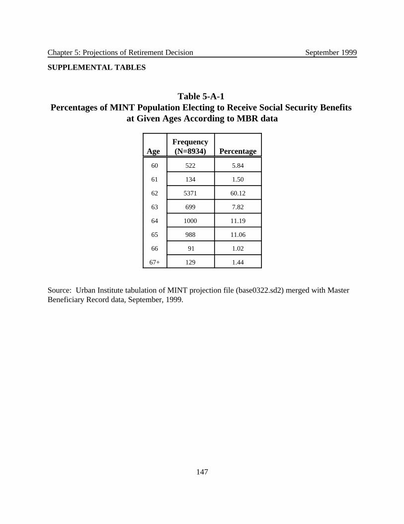
Chapter 5: Projections of Retirement Decision September 1999
147
SUPPLEMENTAL TABLES
Table 5-A-1 Percentages of MINT Population Electing to Receive Social Security Benefits
at Given Ages According to MBR data
AgeFrequency(N=8934) Percentage
60 522 5.84
61 134 1.50
62 5371 60.12
63 699 7.82
64 1000 11.19
65 988 11.06
66 91 1.02
67+ 129 1.44
Source: Urban Institute tabulation of MINT projection file (base0322.sd2) merged with MasterBeneficiary Record data, September, 1999.

Chapter 5: Projections of Retirement Decision September 1999
148
Table 5-A-2Logistic Regression Coefficients:
Social Security Benefit Receipt Timing for Married Men Where no Wealth Variables are Employed
Variable
Parameter Estimate
(Standard Error)(N=2895)
Intercept -2.4717** (0.5372)
Age 63 -1.0951** (0.1277)
Age 64 0.3798** (0.1213)
Age 65 1.4421** (0.1580)
Age 66 -0.2173 (0.2409)
Age 67 -0.8007** (0.2860)
Education < 12 0.1471 (0.1224)
Education > 12 -0.2061 (0.1152)
Non-Hispanic white 0.3615* (0.1457)
Have any pension? 0.2968** (0.1025)
Earnings ages 35-55 1.6563** (0.1425)
Earnings ages 56-61 0.3268** (0.1248)
Earnings at t-1 -1.4460** (0.0981)
Spouse’s age 0.0144 (0.00854)
Spouse’s education < 12 0.0904 (0.1227)
Spouse’s education > 12 -0.0926 (0.1137)
Spouse’s earnings 35-55 0.3806* (0.1502)
Spouse’s earnings at t-1 -0.1941 (0.1107)
* indicates p<.05; ** indicates p<.01

Chapter 5: Projections of Retirement Decision September 1999
149
Table 5-A-3 Logistic Regression Coefficients:
Social Security Benefit Receipt Timing Where Receipt is Capped at Age 69, Rather than Age 67
Parameter Estimate (Standard Error)
Variable Married Men(N=2936 )
Married Women(N=2439)
Unmarried People(N=2390)
Intercept -2.3011** (0.5334) -2.2255** (0.7213) -0.6626** (0.1561)
Age 63 -1.1260** (0.1298) -1.6153** (0.1448) -1.3431** (0.1459)
Age 64 0.3780** (0.1227) -0.5388** (0.1416) -0.4789* (0.1324)
Age 65 1.4739** (0.1609) -0.1283 (0.1760) 0.5669** (0.1511)
Age 66 -0.2500 (0.2474) -1.2103** (0.2457) -1.1357** (0.2246)
Age 67 -0.8490** (0.3001) -1.2333** (0.2531) -0.5800** (0.1964)
Age 68+ -0.1501 (0.2381) -0.9158** (0.1993) -0.9988** (0.1734)
Education < 12 0.1302 (0.1217) -0.0216 (0.1304) 0.1933 (0.1170)
Education > 12 -0.1420 (0.1149) -0.0879 (0.1208) -0.1587 (0.1160)
Non-Hispanic white 0.3218* (0.1437) 0.3074* (0.1422) 0.4723** (0.1128)
Have any pension? 0.2739** (0.1039) -0.3231** (0.1074) 0.0174 (0.1046)
Earnings ages 35-55 1.6772** (0.1432) 1.4546** (0.2392) 0.9950** (0.1691)
Earnings ages 56-61 0.3116* (0.1249) 0.2524 (0.2404) 0.0108 (0.1694)
Earnings at t-1 -1.4041** (0.0977) -1.7043** (0.2134) -0.7537** (0.1339)
Spouse’s age 0.0125 (0.00845) 0.0260* (0.0106)
Spouse’s education < 12 0.1140 (0.1221) 0.2085 (0.1325)
Spouse’s education > 12 -0.0844 (0.1134) -0.0922 (0.1241)
Spouse’s earnings 35-55 0.3484* (0.1494) 1.1499** (0.1023)
Spouse’s earnings at t-1 -0.1525 (0.1096) -0.5278** (0.0685)
Spouse has a pension? 0.1413 (0.1101)
Male -0.1773 (0.1098)
Widowed 0.2030** (0.0973)
Log value of non-housing wealth -0.0204 (0.0513)
Own a home 0.00953 (0.0999)
Value of home -0.0188 (0.0144)
* indicates p<.05; ** indicates p<.01

Chapter 5: Projections of Retirement Decision September 1999
150
Table 5-A-4 Percentages of MINT and Historical (1996) Populations Electing
to Receive Social Security Benefits at Given Ages, by Sex
60 61 62 63 64 65 66 67+
All men in current MINT (weighted) 1.02 0.32 53.12 12.13 17.27 10.74 1.82 3.57
Most similar historical 0.54 0.27 56.70 8.08 11.00 16.93 2.29 4.20
Difference (current MINT-historical) +0.48 +0.05 -3.58 +4.05 +6.27 -6.19 -0.47 -0.63
All women in current MINT (weighted) 7.44 1.96 54.57 8.79 11.68 8.61 2.17 4.78
Most similar historical 8.01 2.24 56.36 6.26 9.04 11.88 1.65 4.55
Difference (current MINT-historical) -0.57 -0.28 -1.79 +2.53 +2.64 -3.27 +0.52 +0.23
MINT Source: Urban Institute tabulation, September, 1999Historical Source: Annual Statistical Supplement, 1997, Tables 6.A4 and 6.D3
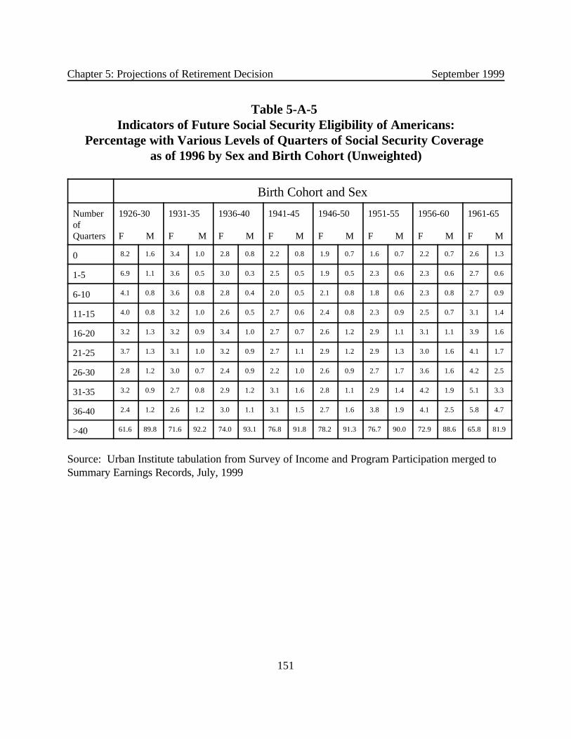
Chapter 5: Projections of Retirement Decision September 1999
151
Table 5-A-5 Indicators of Future Social Security Eligibility of Americans:
Percentage with Various Levels of Quarters of Social Security Coverage as of 1996 by Sex and Birth Cohort (Unweighted)
Birth Cohort and Sex
NumberofQuarters
1926-30
F M
1931-35
F M
1936-40
F M
1941-45
F M
1946-50
F M
1951-55
F M
1956-60
F M
1961-65
F M
0 8.2 1.6 3.4 1.0 2.8 0.8 2.2 0.8 1.9 0.7 1.6 0.7 2.2 0.7 2.6 1.3
1-5 6.9 1.1 3.6 0.5 3.0 0.3 2.5 0.5 1.9 0.5 2.3 0.6 2.3 0.6 2.7 0.6
6-10 4.1 0.8 3.6 0.8 2.8 0.4 2.0 0.5 2.1 0.8 1.8 0.6 2.3 0.8 2.7 0.9
11-15 4.0 0.8 3.2 1.0 2.6 0.5 2.7 0.6 2.4 0.8 2.3 0.9 2.5 0.7 3.1 1.4
16-20 3.2 1.3 3.2 0.9 3.4 1.0 2.7 0.7 2.6 1.2 2.9 1.1 3.1 1.1 3.9 1.6
21-25 3.7 1.3 3.1 1.0 3.2 0.9 2.7 1.1 2.9 1.2 2.9 1.3 3.0 1.6 4.1 1.7
26-30 2.8 1.2 3.0 0.7 2.4 0.9 2.2 1.0 2.6 0.9 2.7 1.7 3.6 1.6 4.2 2.5
31-35 3.2 0.9 2.7 0.8 2.9 1.2 3.1 1.6 2.8 1.1 2.9 1.4 4.2 1.9 5.1 3.3
36-40 2.4 1.2 2.6 1.2 3.0 1.1 3.1 1.5 2.7 1.6 3.8 1.9 4.1 2.5 5.8 4.7
>40 61.6 89.8 71.6 92.2 74.0 93.1 76.8 91.8 78.2 91.3 76.7 90.0 72.9 88.6 65.8 81.9
Source: Urban Institute tabulation from Survey of Income and Program Participation merged toSummary Earnings Records, July, 1999

Chapter 5: Projections of Retirement Decision September 1999
152
Table 5-A-6Indicators of Future Social Security Eligibility of Americans:
Percentage with Various Levels of Quarters of Social Security Coverage as of 1996 by Sex and Birth Cohort (Weighted)
Birth Cohort and Sex
NumberofQuarters
1926-30
F M
1931-35
F M
1936-40
F M
1941-45
F M
1946-50
F M
1951-55
F M
1956-60
F M
1961-65
F M
0 8.8 1.6 3.5 0.8 3.0 0.7 2.2 0.6 1.9 0.7 1.6 0.8 2.2 0.8 2.6 1.3
1-5 6.5 1.1 3.6 0.4 2.9 0.2 2.6 0.4 1.9 0.4 2.1 0.6 2.4 0.8 2.5 0.5
6-10 4.2 0.7 3.4 0.8 2.8 0.4 1.9 0.6 2.1 0.9 1.8 0.6 2.2 0.9 2.6 0.9
11-15 3.6 0.9 3.2 0.9 2.3 0.6 2.7 0.5 2.7 0.7 2.4 0.9 2.5 0.5 3.2 1.2
16-20 3.5 1.3 3.3 0.9 3.8 0.9 2.9 0.7 2.5 1.2 2.4 0.9 3.1 1.0 3.7 1.8
21-25 3.9 1.3 3.3 1.0 3.0 1.1 2.4 1.0 2.8 1.4 2.9 1.2 2.9 1.3 4.0 2.0
26-30 2.9 1.3 2.8 0.6 2.3 0.9 2.2 1.1 2.7 0.9 2.7 1.5 3.4 1.6 4.0 2.0
31-35 3.3 1.0 2.6 0.8 2.7 1.1 2.8 1.5 2.8 1.0 3.0 1.5 4.2 2.2 5.0 3.4
36-40 2.3 1.1 2.4 1.1 2.8 1.2 3.1 1.3 2.3 1.7 3.9 2.0 3.8 2.6 5.8 4.8
>40 60.9 89.9 71.8 92.7 74.5 92.9 77.2 92.3 78.4 91.1 77.3 90.1 73.4 88.1 66.5 82.2
Source: Urban Institute tabulation from Survey of Income and Program Participation merged toSummary Earnings Records, July, 1999

Chapter 5: Projections of Retirement Decision September 1999
153
CHAPTER 5: REFERENCES
Allison, Paul D. 1984. Event History Analysis: Regression for Longitudinal Event Data. Beverly Hills: Sage Publications.
Melissa M. Favreault, Caroline Ratcliffe, and Eric Toder. 1999. “Labor Force Participation ofOlder Workers: Prospective Changes and Potential Policy Responses.” National TaxJournal LIII(3): 483-503.
Social Security Administration, Office of Research, Evaluation and Statistics. 1997. AnnualStatistical Supplement, 1997 to the Social Security Bulletin. Washington, DC: Author.
CHAPTER 5: LIST OF TABLES
Table 5-1Logistic Regression Coefficients Currently Employed in MINT: Social Security Benefit Receipt Timing 132
Table 5-2Percentages of MINT and Historical (1996) Populations Electing to Receive Social Security Benefits at Given Ages
136Table 5-3A
Projected Percentage of MINT Men in Various Demographic and Economic Groups Electing to Receive Social Security Benefits at Given Ages 139
Table 5-3BProjected Percentage of MINT Women in Various Demographic and Economic Groups Electing to Receive Social Security Benefits at Given Ages
140Table 5-A-1
Percentages of MINT Population Electing to Receive Social Security Benefits at Given Ages According to MBR data 147
Table 5-A-2Logistic Regression Coefficients: Social Security Benefit Receipt Timing for Married Men Where no Wealth Variables are Employed 148
Table 5-A-3 Logistic Regression Coefficients: Social Security Benefit Receipt Timing Where Receipt is Capped at Age 69, Rather than Age 67 149
Table 5-A-4 Percentages of MINT and Historical (1996) Populations Electing to Receive Social Security Benefits at Given Ages, by Sex 150

Chapter 5: Projections of Retirement Decision September 1999
154
1. Table 5-A-1 in Appendix A presents estimates of the distribution of ages of first receipt foundin the administrative records. An additional section in the appendix provides a discussion ofmeasurement issues associated with using the administrative and survey data, and estimates of thenontrivial differences in observed outcomes when one uses birth dates from different data sources(self-reports versus administrative reports).
2. Low-earning is defined in terms of the exempt amount for earnings before the NormalRetirement Age. Aggregate data suggest that a deterministic function reasonably approximatesthis process over the historical period. In 1996, nearly a quarter (about twenty-three percent) ofall new benefits for surviving spouses were paid to 60 year-olds (Social Security Administration,1997, Table 6.D7).
Table 5-A-5 Indicators of Future Social Security Eligibility of Americans:Percentage with Various Levels of Quarters of Social Security Coverage as of 1996 by Sex and Birth Cohort (Unweighted) 151
Table 5-A-6Indicators of Future Social Security Eligibility of Americans:Percentage with Various Levels of Quarters of Social Security Coverage as of 1996 by Sex and Birth Cohort (Weighted) 152
CHAPTER 5: LIST OF FIGURES
Figure 5-1 Month of First Benefit Entitlement, Where First Entitlement is Age 60 or Above, Using SIPP and MBR Birthdates 129
Figure 5-A-1 Distribution of Differences Between MBR Ages and SIPP Ages(N=28,732) 146
Figure 5-1 Month of First Benefit Entitlement, Where First Entitlement is Age 60 or Above, Using SIPP and MBR Birthdates 128
Figure 5-A-1 Distribution of Differences Between MBR Ages and SIPP Ages 145
CHAPTER 5: ENDNOTES

Chapter 5: Projections of Retirement Decision September 1999
155
3. This results in part from the structure of MINT, which to a large extent precludes a traditionaleconomic framework of utility maximization. While different aspects of earnings histories andfamily composition included in the equations may suggest some simple optimization rules (e.g.,spouses tend to coordinate their timing decisions), these structures are not explicit.
4. Separate equations by sex for those men and women who were not married at the time theywere at risk of receiving Social Security appeared unnecessary. Coefficient estimates suggest nosignificant differences between men and women in the pooled equation and no significant genderinteraction terms.
5. Because exact months of first Social Security receipt could be determined using the MBR butexact dates could not, we examine individuals in the eleventh month after a birthday. Forexample, if a person was born in November, we checked to see whether he or she received SocialSecurity benefits by the end of October. (The month of analysis is coded as a parameter in theestimation program, even0908.sas, and can be easily modified.) In order to maximize the numberof observations in the analysis, we allowed a person to reach the month before his/her (self-reported) birth month in any month of the survey. This implies that individuals included in theestimation ranged in age from 62 to 67 in the 1989 to 1995 period (and were thus born between1922 and 1933).
6. Estimates of intercepts were usually slightly higher with the screen. This is sensible, since theoverall likelihood of retirement should go up when ineligible individuals are excluded from therisk pool. In later simulations, model users at SSA could adjust the intercepts slightly upward toaccount for this difference, though our provisions for “mandatory” retirement of eligibleindividuals at age 67 should prevent any major problems from this slight discrepancy.
7. Because this function helps to predict earnings at age t, these earnings cannot be used in theequations. To capture lagged earnings in the estimation, we used the annual values from theSummary Earnings Record rather than the monthly levels from SIPP. This is problematic in thatSER earnings at t-1 represent very different things for individuals who were born in January andDecember of the same year. For one person in a given birth cohort, t-1 earnings could representhis/her earnings from eleven months in which he/she was 61 and one month in which he/she was62, while for another person in the same cohort, the same variable would represent earnings fromthe opposite grouping of months.
8. We used pension coverage rather than pension wealth or pension income because the formercan be defined more consistently within MINT. While in theory pension wealth is the mostrelevant of the three variables, the MINT projections of pension wealth/income apply only tothose workers who wait until age 62 before collecting benefits, a restriction we could not easilymake in the SIPP estimation data. Further, using an income indicator in the SIPP data wouldhave led us to confound pension take-up and pension wealth, as information about the value ofdefined benefit pension balances is only available when the person is collecting a pension.

Chapter 5: Projections of Retirement Decision September 1999
156
9. While using multivariate equations like these for projection allows one to capture changes inthe composition of the population into the future, it does not allow one to account for any futurechanges in the underlying structure of a process (in this case, timing of Social Security benefitreceipt). Assuming a constant structure is more problematic when a process is changing rapidlyfor a given group. For married women, the process of Social Security benefit timing has beenchanging in important ways in recent years. With each succeeding cohort, a smaller fraction ofwomen receives benefits as wives and a greater fraction receives benefits as workers. As a result,the relative weights that the SIPP equation for married women attaches to husbands’ and wives’experiences may be less appropriate for future groups of married women.
10. While the equation for married men currently includes two wealth measures, users may wishto omit the wealth measures for this group in future simulations given the coefficients’ lack ofstatistical significance. Table 5-A-2 presents coefficients for married males where these twovariables are omitted.
11. For example, using age minus the Normal Retirement Age rather than age as a predictor inthe equations simply reduces to age, but with a different scale.
12. We could implement either PIA or expected benefit as a predictor quite readily in re-estimating these equations, since we now have a detailed Social Security benefit calculator writtenin SAS. Preliminary estimates, however, indicate that the earnings measures now used in MINTmay provide a better fit than PIA. (Estimates were not made using expected benefits as apredictor.) This does not, however, imply that some other non-linear earnings measure mighthave greater explanatory power than the three earnings measures used here. An indicator variablefor eligibility as a spousal recipient could also potentially improve the model.
13. There are of course complications, and potential disadvantages, to each of theseapproaches. While many of the important predictors of benefit receipt are measured monthly inthe SIPP, the earnings picture could become more muddled using finer gradations. If one wishedto use a person-month rather than person-year specification, one could consider using the SER tocapture permanent earnings, and rely on the SIPP for finer detail on earnings in and close toretirement.
14. The Annual Statistical Supplement for 1998 has been released, but the definition of thepopulation included in Table 6.A4 changed between the 1997 and 1998 editions of theSupplement, rendering the 1998 figures less comparable to the MINT estimates that we presenthere. We therefore rely on data from the 1997 Supplement, which reflect receipt patterns in 1996.
15. Data on newly awarded survivors’ benefit include both new Social Security recipients andspousal recipients who change status upon the death of a spouse. While one can fairly safelyassume that those receiving benefits before age 62 are new Social Security recipients, it is notpossible to distinguish between first-time and other Social Security recipients at higher ages in

Chapter 5: Projections of Retirement Decision September 1999
157
these aggregated statistics. We thus expect some double counting of individuals at higher ages inthese estimates.
16. MINT users at SSA may wish to change this assumption so that non-disabled individualswill be allowed to collect Social Security for the first time in their year of death. They may do soby changing the greater than or equal to sign in the following phrase in the SAS macro “decidret”in the program projectr.sas to a less than sign: if doby+index >= dody then ssage=.;
17. There is a considerable spike in receipt at age 67 among both men and women in the 1926-1930 birth cohorts. We suspect that this may be due to incomplete reporting of receipt of SocialSecurity in the MBR, given that ages of first receipt are derived from the MBR for most membersof these cohorts. As these cohorts are not a part of the core sample, we have nor pursued thisissue.
18. The thresholds for these quintiles, expressed as a percentage of the average wage, are asfollows: 0.19227, 0.49778, 0.83603, and 1.27268.
19. This may be due in part to inaccurate information or mistaken calculations by a householdmember who answers the questionnaire, rather than by the person that the data record describes.

158
CHAPTER 6
PROJECTING PARTIAL RETIREMENT EARNINGS
I. OVERVIEW
This chapter focuses on projecting the work behavior and earnings of 62 and 67 year oldSocial Security beneficiaries. The projections are carried out on a sample of persons born between1931 and 1960 who were Social Security beneficiaries at age 62 and/or age 67. For this sampleof individuals, partial retirement earnings at age 62 are projected to the year 2022 and partialretirement earnings at age 67 are projected to the year 2027.
The projections, which take account of scheduled increases in the Social Security exemptamount between 1996 and 2002, are carried out in two steps. The first step involves estimating astatistical model which captures beneficiaries’ decisions about whether to work and their level ofearnings. This model is estimated with data from the 1984 and 1990-92 panels of the Survey ofIncome and Program Participation (SIPP). The second step uses the estimated coefficients fromthe statistical model as a means of projecting partial retirement earnings of 62 and 67 year olds tothe year 2027.
This chapter first considers the estimation phase, and includes a discussion of the data setand sample, the statistical model, and the estimated coefficients. This is followed by a discussionof the projection methodology and results.
II. ESTIMATING PARTIAL RETIREMENT EARNINGS
1. Data Set and Sample
The estimation of partial retirement earnings is carried out using the 1984 and 1990-92panels of the SIPP. Earnings data from the Social Security Summary Earnings Records (SER)were merged with the SIPP data for all four panels, providing information on covered earningsfrom 1951 through 1996. Additionally, information about (1) the year an individual first receivedSocial Security benefits and (2) whether the individual received disability benefits is obtained fromthe Master Beneficiary Record (MBR) for panels 1984 and 1990-91. The MBR for the 1992SIPP panel was not available at the time the estimation was carried out, so this information wasobtained from self reports as recorded in the 1992 SIPP. The 1984, 1990 and 1991 SIPP panelsprovide two full calendar years of information (1984-85, 1990-91, and 1991-92, respectively),while the 1992 SIPP panel provides three full calendar years of information (1992-94).

Chapter 6: Projecting Partial Retirement Earnings September 1999
159
Rather than estimating the statistical models with only 62 and 67 year olds, we expand theage criteria as a way of increasing the sample size. For the younger group, we include both 62and 63 year olds in the analysis, and for the older group, we include persons ages 65 through 68. A slight data "mismatch" arises regarding individuals' ages because an individual's age is spreadacross two calendar years (except for persons born on January 1), while the Social Security rulesregarding benefit receipt and SER reported earnings are based on a calendar year. In this analysis,we follow people over a calendar year rather than a birth year.
To capture the work behavior of Social Security beneficiaries accurately, we restrict thesample to individuals who are beneficiaries over the entire calendar year. This restriction placesan additional constraint on the calendar year in which we can examine the work behavior of 62year old beneficiaries. Because the majority of individuals are first eligible for benefits at age 62,we analyze the work behavior of 62 year old beneficiaries in the calendar year after their 62ndbirthday. In other words, an individual's age in a particular calendar year is defined as his/her ageon January 1 of that year. For consistency across the sample, the ages of all individuals in thesample are defined similarly.
The discussion of the data below separately considers 62-63 year old beneficiaries and 65-68 year old beneficiaries because the statistical models are estimated separately for these twogroups. One reason for estimating the models separately is that the two populations may behavedifferently, as 62-63 year olds are in the early stages of retirement relative to 65-68 year olds. Asecond reason is that the available data allow us to observe exogenous changes in the exemptamount (relative to the average wage) for persons age 65 through 68, but not for persons age 62through 63. Between 1977 and 1982 there were exogenous increases in the exempt amount forpersons age 65-68. This program difference translates into differences in data availability andspecification of the estimating model. For projection purposes, this information is of particularinterest for 67 year old beneficiaries because the Social Security exempt amount is scheduled toincrease from $14,500 in 1998 to $30,000 in the year 2002 for persons at or above the normalretirement age, but is not scheduled to increase (relative to the average wage) for persons underthe normal retirement age.1
Estimating the partial retirement earnings of 62 and 63 year olds is carried out using the1990-92 panels of the SIPP. Only the most recent 1990-92 data are used for this younger groupof retirees because nothing is gained, in terms of observing ad hoc adjustments to the exemptamount, by using the earlier 1984 data. Focusing on 62-63 year old beneficiaries gives a sampleof persons who were born between 1926 and 1931.2 If an individual meets this age criterion intwo different calendar years, then that individual is included in the sample twice.3 Allowingpersons to enter the sample more than once was done in order to increase the sample size.4

Chapter 6: Projecting Partial Retirement Earnings September 1999
160
Combining the 1990 through 1992 panels of the SIPP in this manner provides a sample of 1,53362 and 63 year olds who are receiving Social Security benefits, of whom 439 (28.6 percent) areworking.5
For persons age 65 through 68 we use the 1990-92 SIPP panels, as well as the 1984 SIPPpanel. The design of the data set from the 1990-92 panels is similar to that described above,where individuals are included in the data set multiple times if they meet the inclusion criteria.6 For the 1990-92 SIPP panels, the sample consists of persons who were born between 1921 and1928.7 The final sample includes 6,138 persons age 65-68 receiving Social Security, of whom1,226 (25.0 percent) are working.
The 1984 SIPP panel is also used for 65-68 year old beneficiaries because it allows us toobserve a time period during which the Social Security exempt amount (relative to the nationalaverage wage) changed for persons in this age group. Between 1977 and 1983 the exemptamount for 65-68 year olds more than doubled, increasing from $3,000 in 1977 to $6,600 in1983.8 While the 1984 SIPP primarily has individuals' information beginning in 1984, the SERdata allow us to observe individuals' earnings during this 1977-83 time period. Thus, we use the1984 SIPP (along with the SER and MBR) to examine Social Security recipients' work behaviorand earnings from 1976 through 1983. The primary difference between the data sets created fromthe 1984 and 1990-92 SIPP panels is that the data set created from the 1984 SIPP does notcontain information on individuals' non-labor income in the same year that earnings are observed(i.e., the information is not coterminous).9 The final sample of persons from the 1984 SIPP wereborn between 1907 and 1917; that is, persons who were age 68-68 in 1976-83. In this case, thesample size was expanded by allowing individuals to be included multiple times. The resultingsample from the 1984 SIPP includes 5,942 Social Security recipients, of whom 1,389 (23.4percent) are working.
Prior research has shown that a large portion of Social Security beneficiaries locate nearor at the exempt amount, and that a relatively small proportion have earnings well above theexempt amount.10 Figures 6-1 through 6-3 present the ratio of earnings to the exempt amountand their relative frequencies for the three samples described above.11
Figure 6-1, which displays information for 65-68 year old beneficiaries from the 1984SIPP, shows that beneficiaries (1) cluster around the point where earnings equals the exemptamount (i.e., the ratio of earnings to the exempt amount equals one) and (2) seldom have earningswell above the exempt amount. Figures 6-2 and 6-3 show a somewhat similar pattern forbeneficiaries in 1990-92, but the clustering around the point where earnings equals the exemptamount is less pronounced. The primary similarity between the three figures is that there are arelatively small number of people with earnings well above the exempt amount.

Chapter 6: Projecting Partial Retirement Earnings September 1999
161
0
20
40
60
80
100
120
140
160
180
0 0.2 0.4 0.6 0.8 1 1.2 1.4 1.6 1.8 2 2.2 2.4 2.6 2.8 3 3.2 3.4 3.6 3.8 4 4.2 4.4 4.6 4.8 5 5.2 5.4
Ratio of Earnings to Exempt Amount
Nu
mb
er o
f P
eop
le
Ratio = 1
Figure 6-1 Ratio of Earnings to Exempt Amount
Persons Age 65 to 68, SIPP 1984

Chapter 6: Projecting Partial Retirement Earnings September 1999
162
0
10
20
30
40
50
60
0 0.2 0.4 0.6 0.8 1 1.2 1.4 1.6 1.8 2 2.2 2.4 2.6 2.8 3 3.2 3.4 3.6 3.8 4 4.2 4.4 4.6 4.8 5 5.2 5.4
Ratio of Earnings to the Exempt Amount
Nu
mb
er o
f P
eop
le
Ratio = 1
Figure 6-2Ratio of Earnings to Exempt Amount Persons Age 65 to 68, SIPP 1990-92

Chapter 6: Projecting Partial Retirement Earnings September 1999
163
0
10
20
30
40
50
60
0
0.2
0.4
0.6
0.8 1
1.2
1.4
1.6
1.8 2
2.2
2.4
2.6
2.8 3
3.2
3.4
3.6
3.8 4
4.2
4.4
4.6
4.8 5
5.2
5.4
Ratio of Earnings to the Exempt Amount
Nu
mb
er o
f P
eop
le
Ratio = 1
Figure 6-3Ratio of Earnings to Exempt Amount Persons Age 62 to 63, SIPP 1990-92

Chapter 6: Projecting Partial Retirement Earnings September 1999
164
2. Estimating Model
In this statistical analysis, we estimate two models. We began with a two-equation model,where the first equation incorporates the decision to work or not work, and the second equationestimates the level of earnings for those individuals who work. This first model is referred to asthe probit/earnings model.12 In preliminary analyses, we found that the second stage earningsequation had very limited explanatory power. In other words, the observable characteristics ofworking beneficiaries provide little information about their earnings levels.
In the earnings equations for both young (62-63) and old (65-68) working beneficiaries,none of the coefficients for demographic variables (such as age, marital status, educationalattainment) were statistically significant at the 10 percent level of significance. For the olderbeneficiaries, a few of the economic variables had statistically significant effects, but none of thesevariables had statistically significant effects for the younger beneficiaries.13 The limitedexplanatory power of the earnings equations, particularly for younger beneficiaries, makes itdifficult to obtain reliable earnings projections.
The limited ability of the probit/earnings model to explain working beneficiaries level ofearnings led us consider an alternate modeling approach. Rather than predicting individuals’ levelof earnings, we predict “roughly” where on the earnings distribution an individual will fall. To dothis we use an ordered probit model.14 To estimate this model, the earnings distribution is dividedinto four segments, where the break points are based on the information provided in Figures 6-1through 6-3. These segments are: (1) no earnings, (2) earnings greater than 0 but less than 85percent of the exempt amount (0 < ratio of earnings to the exempt amount < 0.85), (3) earningsbetween 85 percent and 115 percent of the exempt amount (0.85 # ratio of earnings to theexempt amount # 1.15), and (4) earnings greater than 115 percent of the exempt amount (ratio ofearnings to the exempt amount > 1.15). The estimated coefficients from the ordered probit modelallow us to project where on the earnings distribution future beneficiaries will fall. This approach,however, does not have a second stage earnings equation, so in the projection phase earnings areassigned randomly.15
For 62-63 year old beneficiaries, the probit/earnings and ordered probit models wereestimated using the 1990-92 SIPP data. For 65-68 year olds there are multiple options becausetwo data sets were created -- one with the 1984 SIPP and one with the 1990-92 SIPP. The 1984SIPP is of significant value because it can be used to exploit the exogenous increases in the SocialSecurity exempt amount that occurred between 1977 and 1983. That is, we can estimate theeffect of an increase in the exempt amount on the earnings of beneficiaries aged 65-68 using the1984 SIPP data. One option is to use only the 1984 SIPP to estimate the earnings of 65-68 yearold beneficiaries. However, as described previously, using the 1984 SIPP data in this way has adrawback. Detailed coterminous data on several key explanatory variables are not available(these variables include IRA, 401k, and Keogh account balances, pension income, and wealth).

Chapter 6: Projecting Partial Retirement Earnings September 1999
165
We address this issue by estimating the models for 65-68 year olds separately on the 1984SIPP and the 1990-92 SIPP data sets, and then using the information from both analyses in theprojection. Combining information from models estimated with the 1984 SIPP data and the 1990-92 SIPP data may provide the most complete set of information for projection purposes. In thiscase, we do the following: (1) estimate the model using the 1984 SIPP, where the exempt amountis one of the explanatory variables and (2) estimate the model using the 1990-92 SIPP data, wherethe coterminous variables are among the explanatory variables. With this approach, the projectionis carried out using the estimated coefficient on the exempt amount obtained from the analysisusing the 1984 SIPP, and all other estimated coefficients come from the models estimated withthe 1990-92 SIPP data.16
For older beneficiaries, we estimate both the probit/earnings and ordered probit modelswith the 1984 and 1990-92 SIPP data sets. With the 1984 SIPP, we estimate an additional threeearnings equations, where the ranges of earnings are defined by break points used in the orderedprobit model.17 We estimate these additional earnings equations to obtain additional informationregarding how a $1 increase in the exempt amount affects beneficiaries' earnings.
Information obtained from estimating the probit/earnings models with the 1990-92 SIPP(for both older and younger beneficiaries) was not used in the projection phase, so these modelsare not discussed in detail. See Appendix 6-B for the results from these models. The focus of thediscussion below is on the following models:
C 62-63 Year Old Beneficiaries, 1990-92 SIPP: Ordered probit modelC 65-68 Year Old Beneficiaries, 1990-92 SIPP: Ordered probit modelC 65-68 Year Old Beneficiaries, 1984 SIPP: Probit/earnings model, ordered probit model,
plus other earnings equations.
The explanatory variables included in the models are listed below (interactions betweensome of these variables are also included in the models).18
In the ordered probit and probit models the explanatory variables are:
C Social Security exempt amount (1984 only)
C average earnings (two measures): age 35-55 and age 56-61 (1990-92, 62-63 year olds)/age 35-59 and age 60-64 (1990-92, 65-68 year olds)/ age 45-59 and age 60-64 (1984)19
C family pension income (1990-92 only)
C family wealth (1990-92 only)
C family balance of IRA, 401k, and Keogh accounts (1990-92 only)
C indicators of age

Chapter 6: Projecting Partial Retirement Earnings September 1999
166
C indicator of whether the individual is non-Hispanic white
C indicator of whether the individual has less than a high school education
C indicator of whether the individual has a high school education only
C indicator of the individuals' gender and marital status20
C spouse’s age (where applicable)
and in the earnings equation estimated with the 1984 SIPP the explanatory variables are:
C Social Security exempt amount
C average earnings: age 60-6421
C indicators of age
The results of the models are presented in the following order: (1) 62-63 year oldbeneficiaries using the 1990-92 SIPP, (2) 65-68 year old beneficiaries using the 1990-92 SIPP,and (3) 65-68 year old beneficiaries using the 1984 SIPP. Recall that in the ordered probit,individuals are placed into four groups:
Group 0: No earnings.Group 1: Earnings greater than 0 but less than 85 percent of the exempt amount.Group 2: Earnings between 85 percent and 115 percent of the exempt amount.Group 3: Earnings greater than 115 percent of the exempt amount.
Ordered Probit Model Results for 62-63 Year Old Beneficiaries, 1990-92 SIPP
The explanatory variables in the ordered probit model for 62 year old beneficiaries includethose variables listed in the previous section. This model, however, distinguishes between marriedfemale beneficiaries and all other beneficiaries. Specification tests revealed that married femalesbehave differently with regard to post-retirement employment and earnings, as compared tounmarried persons and married males. In addition to including a variable indicating whether anindividual is a married female, married female status is interacted with several other explanatoryvariables.
The ordered probit model presented in Table 6-1 was estimated on a sample of 1,533persons, where 1,094 persons are in earnings group 0, 300 are in earnings group 1, 94 are inearnings group 2, and 45 are in earnings group 3. The model includes 13 explanatory variables,of which eight have effects statistically different from zero at the 5 percent level (P-values lessthan 0.05), but the other five variables do not have statistically significant effects at even the 10

Chapter 6: Projecting Partial Retirement Earnings September 1999
167
Table 6-1Ordered Probit Modela
Social Security Beneficiaries Age 62 to 63, 1990-92 SIPP
Ordered ProbitExplanatory Variable (obs=1,533)
Non-Hispanic White 0.1549 (0.1015)
Education Less than 12th Grade -0.3413 ** (0.0955)
Education Equal to 12th Grade -0.1011 (0.0843)
Age 63 -0.0657 (0.0682)
Married Female -0.4693 ** (0.1183)
Married Female * Spouse Age -0.0334 ** (0.0159)
Family Wealthb -0.0023 (0.0053)
Family Pension Benefits -0.7562 ** (0.1348)
Family Pension * Married Female 0.4393 ** (0.1904)
Family Retirement Balances (IRA, 401k, Keogh) -0.0209 (0.0391)
Average Past Earnings (ages 35-55) -0.1772 ** (0.0897)
Average Recent Earnings (ages 56-61) 0.4913 ** (0.0886)
Average Recent Earnings * Married Female 0.5721 ** (0.1898)
Pseudo R-square 0.0580
Chi-squared 148.36 (df=13)
Cutoff value 1 0.2870 (0.1346)
Cutoff value 2 1.1194 (0.1371)
Cutoff value 3 1.7111 (0.1450)
a) These groups are: Group 0, no earnings; Group 1, earnings greater than 0 but less than 85 percent of theexempt amount; Group 2, earnings between 85 percent and 115 percent of the exempt amount; and Group 3,earnings greater than 115 percent of the exempt amount.
b) Family wealth, family pension benefits, average past earnings, and average recent earnings are divided bynational average earnings.
c) Standard errors in parentheses.
d) Significance at 5 percent is represented by "**".

Chapter 6: Projecting Partial Retirement Earnings September 1999
168
percent level. Of these five coefficients, three have P-values ranging between 0.13 and 0.34, andtwo measures of a family's financial well-being -- family wealth and family retirement balances --have significantly higher P-values of about 0.65. Coefficients for both of these financial well-being variables have the expected sign, so we have chosen to keep them in the model.
Coefficients from an ordered probit equation are somewhat difficult to interpret, but theydo produce some important unambiguous results. One such result is that a positive coefficientindicates that an increase in the explanatory variable will cause the probability of working to riseand a negative coefficient indicates that an increase in the explanatory variable will cause theprobability of working to decline.
Discussion of the results for the younger beneficiaries focuses first on the variables foundto have statistically significant effects at the 5 percent level. Starting with the demographicvariables, the model results suggest that persons with less than a high school education are lesslikely to work than persons with more than a high school education. We also find that marriedfemale beneficiaries are less likely to work than other beneficiaries. Married female status isinteracted with the spouse's age and the estimated coefficient suggests that women who aremarried to older men are less likely to work than women who are married to younger men, all elsebeing equal. The model does not include an interaction between spouse's age and married malestatus because spouse's age was not found to influence significantly the behavior of married men.
The model suggests that higher pension benefits reduce the probability of working. Thisreduction, however, is smaller for married females than for other beneficiaries. This smaller effectfor married females is evident from the positive and statistically significant coefficient on theinteraction term between pension benefit level and the indicator of married female status.
Table 6-1 also shows that while beneficiaries with higher average recent earnings (betweenages 56 and 61) are more likely to work, the positive (and large) coefficient on the interactionterm of recent earnings and married female status suggests that recent earnings play a larger rolein the work decision of married female beneficiaries. Although higher average recent earnings(ages 56 to 61) is found to increase the probability of working, higher average past earnings (ages35 to 55) is found to decrease the probability of working. A comparison of these two coefficientsshows that the negative impact of past earnings is substantially smaller than the positive impact ofmore recent earnings.
For the five variables with effects that are not statistically different from zero, yet areincluded in the projection component, we find the following: (1) non-Hispanic white beneficiariesare more likely to work than minority beneficiaries, (2) beneficiaries with a high school degree(only) are less likely to work than beneficiaries with more than a high school degree, (3) 63 yearold beneficiaries are less likely to work than 62 year old beneficiaries, (4)

Chapter 6: Projecting Partial Retirement Earnings September 1999
169
higher wealth holdings reduce the probability of working, and finally, (5) higher retirementaccount balances (IRA, 401k, and Keogh) reduce the probability of working.
The relatively large number of explanatory variables with significant effects is reflected inthe chi-squared statistic. The chi-squared statistic has a value of 148.36, and with 13 degrees offreedom it is well above the critical value of 22.36. Since this is not a linear model, we cannotcompute an R-squared value. However, we have calculated a pseudo-R-squared statistic. Thiscalculation is based on the log-likelihood value in the estimated model (the "restricted" model)and the log-likelihood value in a model with only a constant (the "unrestricted" model).22 In thisordered probit model, the value of this pseudo-R-squared is 0.058.
Ordered Probit Model Results for 65-68 Year Old Beneficiaries, 1990-92 SIPP.
For the older beneficiaries (age 65-68), we have more flexibility because the sample size issubstantially larger (6,138 versus 1,533).23 The estimated coefficients from the preliminaryordered probit models suggest that married beneficiaries are less likely to work than unmarriedbeneficiaries, so we split the sample by marital status and estimated two separate equations. Theestimation of identical model specifications for unmarried beneficiaries and married beneficiariesresulted in coefficient estimates that were quite different, providing evidence that splitting thesample is preferred. An indicator variable for gender was included in these two models, and thecoefficient estimates suggest that unmarried males and females are similar, while married malesand females differ. As a result, we further split the sample of married persons into married malesand married females. The net result is that, for older beneficiaries, we estimate three separateordered probit equations -- one for unmarried persons (n=1,831), a second for married males(n=2,121), and a third for married females (n=2,186).
The models estimated for older beneficiaries include explanatory variables that were takenfrom the set of variables included for younger beneficiaries. Variables with highly insignificantcoefficients were omitted from the estimation equation because these coefficients have a highprobability of being zero, and therefore, we do not want to include them in the projection phase. As a result, the estimation equations for the three groups do not have the same set of explanatoryvariables. The estimated coefficients are presented in Table 6-2. The results are presented firstfor unmarried persons, then for married males, and finally, for married females.
Unmarried Beneficiaries: The model for unmarried beneficiaries includes nineexplanatory variables, of which five have statistically significant effects at the five percent leveland one has statistically significant effects at the 10 percent level. The statistically significantcoefficients include those for an indicator of whether the individual has less than a high schooleducation, three indicator variables for beneficiaries’ ages, family pension benefits, and average

Chapter 6: Projecting Partial Retirement Earnings September 1999
170
Unmarried People Married Males Married FemalesExplanatory Variable (n=1,831) (n=2,121) (n=2,186)
Education Less than 12th Grade -0.3766 ** (0.0885) -0.2947 ** (0.0661)Education Equal to 12th Grade -0.1127 (0.0842)
Spouse's Age -0.0171 ** (0.0052) -0.0126 (0.0081)
Age 66 -0.1770 * (0.0955)Age 67 -0.2572 ** (0.0940) -0.1800 ** (0.0717) -0.1516 * (0.0881)Age 68 -0.3177 ** (0.0942) -0.3171 ** (0.0729) -0.2836 ** (0.0959)
Family Wealth b -0.0002 (0.0094) -0.0007 (0.0046)Family Pension Benefits -1.2946 ** (0.1836) -0.6591 ** (0.0807) -0.3996 ** (0.0964)
Average Past Earnings (ages 35-59) -0.1109 (0.0957) -0.5460 ** (0.0769)Average Recent Earnings (ages 60-64) 1.0328 ** (0.0885) 0.7097 ** (0.0531) 1.4470 ** (0.0920) Pseudo R-squared 0.0913 0.0845 0.1283Chi-squared 229.98 (df=9) 278.02 (df=8) 257.74 (df=5)Cutoff value 1 0.5757 (0.1042) -1.0196 (0.3316) 0.3831 (0.5565)Cutoff value 2 1.4070 (0.1104) -0.0222 (0.3315) 1.3188 (0.5586)Cutoff value 3 1.7707 (0.1180) 0.3688 (0.3326) 1.7084 (0.5616)
a) These groups are: Group 0, no earnings; Group 1, earnings greater than 0 but less than 85 percent of the exempt amount; Group 2, earnings
between 85 percent and 115 percent of the exempt amount; and Group 3, earnings greater than 115 percent of the exempt amount.b) Family wealth, family pension benefits, average past earnings, and average recent earnings are measured relative to national average earnings.c) Standard errors in parenthesis.d) Significance at 5 percent is represented by "**".
e) Significance at 10 percent is represented by "*".
Table 6-2Ordered Probit Model by Marital Status and Gendera
Social Security Beneficiaries Age 65 to 68, 1990-92 SIPP

Chapter 6: Projecting Partial Retirement Earnings September 1999
171
recent earnings. The coefficients on these six variables indicate the following with respect to thework behavior of unmarried beneficiaries: (1) beneficiaries with less than a high school educationare less likely to work than beneficiaries with more than a high school education, (2) beneficiariesbetween the ages of 66 and 68 are less likely to work than 65 year old beneficiaries, (3)beneficiaries with higher pension benefits are less likely to work, and (4) beneficiaries with higheraverage earnings between the ages of 60 and 64 are more likely to work.
The effect of the indicator variable for whether the beneficiary has a high school degree(only) is not statistically significant at conventional levels, but it remains in the model because theP-value is not particularly high (0.18) and the coefficient has the expected sign (negative). Also,the magnitude of the coefficient is reasonable in that it suggests that individuals with a high schooldegree (only) have (1) a lower probability of working as compared to beneficiaries with more thana high school degree, but (2) a higher probability of working as compared to individuals with lessthan a high school degree. The coefficient on average past earnings (age 35-59) has a somewhathigher P-value (0.25), but remains in the model. The negative sign on this coefficient is consistentwith the findings for younger beneficiaries; while higher recent earnings increase the probabilityof working, higher past earnings decrease the probability of working.
The coefficient on family wealth is small (negative) and not statistically significant. Estimating the model with an alternative measure of wealth -- family income from assets --produces a negative and statistically significant (at the 10 percent level) coefficient. The finalmodel, however, does not include income from assets because this variable is measured differentlyin the SIPP data set than in the MINT projection data set. Because wealth, when measured interms of income from assets, has statistically significant effects, we chose to keep the wealthvariable in the model even if, as measured, its effects are highly insignificant. The negativecoefficient on the wealth variable suggests that beneficiaries with a higher level of wealth are lesslikely to work.
In addition to this model for unmarried beneficiaries, we estimated another, similar model,with the addition of a variable capturing family retirement account balances (i.e., 401(k), IRA, andKeogh). The results of this model, presented in Appendix 6-D Table 6-D-1, suggest that personswith higher 401(k), IRA, and Keogh account balances are more likely to work (significant at thefive percent level). While these retirement account balances were found to increase theprobability of working, family wealth and pension benefit levels were found to have the oppositeeffect. One explanation for this apparently anomalous result is that persons with high accountbalances are likely to be self-employed, particularly because this measure includes Keoghaccounts. The positive and significant coefficient may be therefore picking up a self-employmenteffect instead of an effect of higher retirement account balances. Because individual contributionsto retirement accounts are increasing and a larger percentage of contributions in the future will befor employees (rather than the self-employed), this estimated positive relationship betweenaccount wealth and working is not likely to persist. Therefore, our final projections for olderbeneficiaries exclude the effect of these retirement accounts.24

Chapter 6: Projecting Partial Retirement Earnings September 1999
172
For this model, the chi-squared statistic has a value of 229.98, which is well above thecritical value of 16.92 (9 degrees of freedom). This is not a linear model, so we compute apseudo-R-squared statistic rather than an R-squared value. In this model, the value of thepseudo-R-squared is 0.091.
Married Male Beneficiaries: The estimated coefficients from the ordered probit modelfor married male beneficiaries are presented in column 2 of Table 6-2. Unlike the model forunmarried beneficiaries, this model excludes an indicator of educational attainment equal to highschool and an indicator variable for age 66. These variables are excluded because their effects arehighly insignificant.25
The results for married males are similar to those found for unmarried persons, althoughthe former model includes an indicator of the spouse’s age. The results suggest that the workdecision of married male beneficiaries is influenced by the age of their wife. Men who are marriedto younger women are more likely to work in retirement, as compared to men who are married toolder women. Recall that in the model for younger beneficiaries we found that married men'swork decisions were not affected by their wives’ age.
Married Female Beneficiaries: The third model considers the work behavior of marriedfemale beneficiaries (see column 3 of Table 6-2). In this model we include only five explanatoryvariables -- indicator variables for age 67 and age 68, family pension benefits, average recentearnings, and age of the spouse. The results of this model, in terms of the signs of the coefficients,suggest that (1) beneficiaries are less likely to work as they get older, (2) higher pension benefitslead to a lower probability of working, (3) beneficiaries with higher recent earnings are morelikely to work, and (4) female beneficiaries married to older men are less likely to work.
Average past earnings (age 35-59) and the indicators of educational attainment and ageare not included in the list of explanatory variables because they have highly insignificant effects.26 The family wealth variable is excluded from the model for two reasons. First, neither thecoefficient on family income from assets nor family wealth is statistically different from zero. Inaddition, the coefficients on these two variables are of opposite signs, making the direction inwhich wealth affects the post-retirement work decision at age 67 ambiguous.
As was the case with the other models, the chi-squared statistic for these two models(married males and married female) is well above the critical value. The pseudo-R-squared is0.085 for the married male model and 0.128 for the married female model.
Results for 65-68 Year Old Beneficiaries Using the 1984 SIPP.
Models estimated with the 1984 SIPP include the (1) probit/earnings model, (2) orderedprobit model, and (3) three additional earnings equation. The additional earnings equations are

Chapter 6: Projecting Partial Retirement Earnings September 1999
173
estimated as a means of obtaining more information about how a one dollar increase in the exemptamount affects beneficiaries earnings. These three models are discussed in turn below.
The two-equation probit/earnings model is presented in Table 6-3.27 Recall that the firstequation incorporates the decision to work or not work, and the second equation estimates thelevel of earnings for those individuals who work. In the work/no work equation, the coefficienton the Social Security exempt amount is negative, but the coefficient is not statistically differentfrom zero. A negative coefficient on this variable would suggest that an increase in the exemptamount reduces the probability that an individual will work (not the expected sign). In theearnings equation, however, the coefficient on the exempt amount is positive and statisticallydifferent from zero at the one percent level of significance, suggesting that an increase in theexempt amount increases the earnings of working beneficiaries. The estimated coefficient of0.466 suggests that a one dollar increase in the exempt amount will in turn increase the earningsof working beneficiaries by 46.6 cents. Overall, this model suggests that the Social Securityexempt amount does not influence beneficiaries' decisions about whether to work, but doesinfluence their decisions about how much to earn.
The next model that we consider is the ordered probit model, which is presented in Table 6-4. The estimated coefficient on the Social Security exempt amount from this ordered probit model is negative and is not statistically significant, as in the probit model.28 If we look only atthe ordered probit results, we would conclude that the Social Security exempt amount does notinfluence beneficiaries earnings behavior. The results of the probit/earnings model, however,suggest otherwise.
Because the probit/earnings model result indicating that an increase in the Social Securityexempt amount increases the earnings of working beneficiaries is strong (i.e., the coefficient onthe exempt amount in the earnings equation is significant at the one percent level), we choose toincorporate this information into the projection phase. That is, the projection phase will be suchthat the Social Security exempt amount does not influence beneficiaries' decisions about whetherto work, but does influence their decisions about how much to earn.
The projections could be carried out using the estimated coefficient from the earningsequation which suggests that a one dollar increase in the exempt amount leads to a 46.6 centincrease in the earnings of working beneficiaries. One drawback of this approach is that allworking beneficiaries' earnings are assumed to be identically affected by a given increase in theSocial Security exempt amount. For example, if the exempt amount increases by 10 dollars, theearnings of all working beneficiaries will rise by $4.66, regardless of whether that beneficiary hasearnings well below the exempt amount or at the exempt amount.

Chapter 6: Projecting Partial Retirement Earnings September 1999
174
Probit Earnings Explanatory Variable (obs=5942) (obs=1389)
Social Security Exempt Amount -0.3929 (0.4243) ** 0.4663 (0.2005)
Non-Hispanic white ** -0.1429 (0.0570)Education less than 12th grade **-0.1410 (0.0509)Education equal to 12th grade 0.0445 (0.0546)Male ** 0.2290 (0.0456)
Age 66 ** -0.1012 (0.0506) -0.0207 (0.0228)Age 67 ** -0.1964 (0.0517) -0.0209 (0.0243)Age 68 ** -0.2882 (0.0529) -0.0203 (0.0261)
Average past earnings (ages 45-59) ** -0.1881 (0.0692)Average recent earnings (ages 60-64) ** 0.6527 (0.0593) ** 0.1971 (0.0264)
Constant 0.1216 (0.0941) ** -0.6199 (0.1782)
Inverse Mills Ratioa -0.0917 (0.0809)
Pseudo R-squared/R-squaredb 0.06130 0.1093
Chi-squared / F-statisticc 395.92 (df = 10) 17.93 (df= 6, 1382)
a) The inverse mills ratio is the correction term as described in appendix A.b) Pseudo R-squared calculated for ordered probit and R-squared calculated for earnings equations.c) Chi-squared calculated for the ordered probit and F-statistic calculated for the earnings equations.d) Standard errors in parenthesis.e) Significance at 10 percent is represented by "*".f) Significance at 5 percent is represented by "**".
Table 6-3Probit/Earnings Model
Persons Age 65 to 68, SIPP 1984

Chapter 6: Projecting Partial Retirement Earnings September 1999
175
Ordered Probit
Explanatory Variable (obs=5,942)
Social Security Exempt Amount -0.5619 (0.4061)
Non-Hispanic white ** -0.1222 (0.0547)Education less than 12th grade ** -0.1540 (0.0476)Education equal to 12th grade 0.0066 (0.0511)Male ** 0.2251 (0.0440)
Age 66 ** -0.1107 (0.0482)Age 67 ** -0.1970 (0.0492)Age 68 ** -0.3030 (0.0507)
Average past earnings (ages 45-59) ** -0.2067 (0.0663)Average recent earnings (ages 60-64) ** 0.7134 (0.0567)
Pseudo R-squared 0.0533Chi-squared 480.51 (df=10)
Cutoff value 1 0.5710 (0.1705)Cutoff value 2 1.2527 (0.1711)Cutoff value 3 1.7028 (0.1722)
a) Standard errors in parenthesis.b) Significance at 10 percent is represented by "*".c) Significance at 5 percent is represented by "**".
Table 6-4Ordered Probit Model
Social Security Beneficiaries Age 65 to 68, 1984 SIPP

Chapter 6: Projecting Partial Retirement Earnings September 1999
176
It is unlikely that beneficiaries at different point of the earnings distribution are similarlyaffected by changes in the Social Security exempt amount, so we split the earnings distributioninto three segments and estimate a separate earnings equation for each segment: the first earningsequation includes beneficiaries with earnings greater than 0 but less than 85 percent of the exemptamount, the second earnings equation includes beneficiaries with earnings between 85 percent and115 percent of the exempt amount, and the third earnings equation includes beneficiaries withearnings greater than 115 percent of the exempt amount. The results of these three earningsequations are presented in Table 6-5.
In all three of the earnings equations, the coefficient on the exempt amount is positive,suggesting that an increase in the exempt amount increases the earnings of working beneficiaries. The estimated coefficients and standard errors from the earnings equations suggest that thesecoefficients are statistically different from zero. The coefficient estimates suggest that a $1increase in the exempt amount will increase earnings by (1) $0.25 for beneficiaries with earningswell below the exempt amount (group 1), (2) $0.94 for beneficiaries with earnings in the near orat the exempt amount (group 2), and (3) $1.44 for beneficiaries with earnings over the exemptamount (group 3).29 While we would not expect the value for this last group to be greater than$1, we cannot reject the null hypothesis that a $1 increase in the exempt amount increases theearnings by $1. This is because the standard error on the coefficient is relatively large -- thecoefficient is 1.44 and the standard error is 0.50. These are estimates that are included in theprojection phase.
III. PROJECTING PARTIAL RETIREMENT EARNINGS
1. Procedure Used to Project Partial Retirement Earnings
Partial retirement earnings are projected using a sample of individuals from the 1990-1993SIPP panels who were born between 1931 and 1960. These projections are carried out using thesubset of individuals who are Social Security beneficiaries (see Chapter 5). Other MINTprojections used here include those for mortality, marital status, covered earnings, non-pensionwealth, pension benefits, and IRA, 401(k) and Keogh account balances.
The projections are carried out in two steps. The first step is to determine into which ofthe four earnings groups individuals fall. This placement is based on the interaction betweenindividual characteristics and the estimated coefficients from the ordered probit model. Thesecond step is to assign working beneficiaries' a level of earnings. Because the earnings equationsfor working beneficiaries have little explanatory power, the earnings of working beneficiarieswithin these groups are assigned based only on a random number and a fixed distribution ofearnings (from the 1990-1992 SIPP), not on individual characteristics.

Chapter 6: Projecting Partial Retirement Earnings September 1999
177
Earnings, Group 1 Earnings, Group 2 Earnings, Group 3
0< ratio < 0.85a 0.85<= ratio <=1.15a ratio >1.15a
Explanatory Variable (obs=871) (obs=290) (obs=228)
Social Security Exempt Amount ** 0.2532 (0.0702) ** 0.9424 (0.0308) ** 1.4448 (0.4959)
Age 66 0.0139 (0.0095) -0.0037 (0.0044) -0.0517 (0.0609)Age 67 0.0016 (0.0108) 0.0036 (0.0050) 0.0449 (0.0786)Age 68 * 0.0232 (0.0129) 0.0011 (0.0061) * 0.1764 (0.0910)
Average past earnings (ages 45-59) Average recent earnings (ages 60-64) 0.0139 (0.0212) -0.0011 (0.0102) 0.2146 (0.1409)
Constant 0.0473 (0.0405) 0.0324 (0.0262) -0.1648 (0.1956)
Inverse Mills Ratiob -0.0097 (0.0292) -0.0157 (0.0133) ** 2.2050 (0.9017)
R-squared 0.0288 0.7256 0.3152F-statistic 5.06 (df= 6, 864) 165.62 (df= 6, 283) 11.9 (df= 6, 221)
a) Ratio is defined as earnings divided by the exempt amount.b) This inverse mills ratio is "adjusted" to take account of the fact that individuals who enter each of the the earnings groups are a select group of individuals. c) Standard errors in parenthesis.d) Significance at 10 percent is represented by "*".e) Significance at 5 percent is represented by "**".
Table 6-5Earnings Equations for Working Beneficiaries, by Earnings Group
Social Security Beneficiaries Age 65 to 68, 1984 SIPP
Projecting Individuals' Earnings Group
These projections are based on the estimated coefficients from the ordered probit models.We multiply the individual characteristics of each beneficiary on the MINT file ( ) by theXiestimated coefficients ( ). The resulting value ( ) is used to calculate, for each individual, the$̂ Xi$̂predicted probability of falling into each of the four earnings groups. The predicted probabilitiesare based on the normal distribution and are defined as follows:
Probability Earnings Group 0: M(cutoff value 1 & Xi$̂)
Probability Earnings Group 1: - M(cutoff value 2 & Xi$̂) M(cutoff value 1 & Xi$̂)
Probability Earnings Group 2: - M(cutoff value 3 & Xi$̂) M(cutoff value 2 & Xi$̂)
Probability Earnings Group 3: 1 - M(cutoff value 3 & Xi$̂)

Chapter 6: Projecting Partial Retirement Earnings September 1999
178
The cutoff values 1-3 are presented, along with the estimated coefficients, in Tables 6-1 and 6-2.
To determine in which of the four earnings groups an individual will be placed, wecompare the newly calculated predicted probabilities to a random draw probability from a uniformdistribution (between 0 and 1). The following example helps highlight this process. Suppose thatthe calculated probabilities for an individual are as follows:
Predicted probability of group 0 is 0.532 (cumulative probability equals 0.532)Predicted probability of group 1 is 0.251 (cumulative probability equals 0.783)Predicted probability of group 2 is 0.148 (cumulative probability equals 0.931)Predicted probability of group 3 is 0.069 (cumulative probability equals 1.000)
If the random draw is 0.456, then the individual is placed into group 0, because the random drawis lower than the predicted probability of being in group 0. However, if the random draw is 0.900then the individual is placed into group 2, because the random draw falls above the group 1cumulative probability but falls below the group 2 cumulative probability.
To impose consistency in individuals’ earnings trajectories, we use the same random drawfor both the age 62 and age 67 projections.
Projecting Individuals' Level of Earnings
As mentioned above, working beneficiaries' projected earnings are not based on individualcharacteristics, but are based on a (second) random draw and a fixed distribution of earnings. Forthe projections carried out here, the distribution of earnings is taken from the 1990-92 SIPPestimation data set.30 Because individuals are placed into one of three earnings groups with non-zero earnings, the level of earnings from the SIPP data has been divided intothree separate data sets. For example, individuals placed into earnings group 1 will be randomlyassigned a level of earnings from the earnings of group 1 beneficiaries in the 1990-92 SIPPestimation data set.
In assigning working beneficiaries a level of earnings, the first step is to look at theindividuals' assigned earnings group. Based on this assigned earnings group, the (SAS) programpoints to the appropriate earnings data set and based on a (second) random draw from a uniformdistribution, the individual is assigned a level of earnings based on that draw. The level ofearnings in these three separate SAS data sets are sorted from low to high, so a person with a low random draw will be assigned low earnings (relative to that group) and a person with a higherrandom draw will be assigned high earnings (relative to that group).31

Chapter 6: Projecting Partial Retirement Earnings September 1999
179
2. Projections for 62 Year Old Beneficiaries
Projected Earnings Group
Overall, the results of our projections suggest that a higher fraction of 62 year oldbeneficiaries will be employed over the next two decades than the fraction of beneficiariescurrently employed, as calculated from the 1990-92 SIPP. Table 6-6 presents a comparison ofcalculations from the 1990-92 SIPP (the "current" data) and MINT projection file (the"projected" data) by earnings group and marital status/gender. Calculations from the current datashow that 70.4 percent of beneficiaries are not employed (i.e., in earnings group 0), whereas theprojections based on the MINT file indicate that only 60.7 percent of beneficiaries will not workover the next few decades -- a difference of 10 percentage points.32
A comparison of these percentages by marital status and gender shows that the largestdifference is for married females. While the projections suggest that 32.7 percent of marriedfemale beneficiaries will work (or 67.3 percent will not work), in the current data only 21.2percent work. This difference of almost 12 percentage points is, in part, due to an increase in thepre-retirement employment of married women. While pre-retirement employment is not explicitlytaken into account in our model, the model does incorporate individuals' earnings. Averagerecent earnings (divided by national average earnings) for married females has a mean value of0.20 in the current data and has a significantly higher mean of 0.51 in the MINT projection dataset.
The findings also suggest that married male beneficiaries and unmarried beneficiaries aremore likely to be employed over the next few decades, but their increase in employment is lessthan for married females. The projections suggest that 43.7 percent of married male beneficiarieshave non-zero earnings, while calculations based on the current data show that 35.1 percent havenon-zero earnings, an increase of 8.6 percentage points. For unmarried persons, the increase is8.2 percentage points.
Table 6-6 also compares the current and projected percentage of 62 year old beneficiariesin earnings groups 1 through 3, by marital status and gender. Columns 3 through 8 of the tableshow that the projected results place a higher fraction of beneficiaries into each of the threepositive earnings groups (earnings group 1-3), as compared to the current estimates. Differencesbetween the current and projected values range from 0.6 percentage points to 6.9 percentagepoints.
Tables 6-7 through 6-10 examine beneficiaries’ work behavior by cohort. Beneficiariesborn between 1931 and 1960 are placed into one of six cohort groups, where the cohort groupsare in five-year increments. Looking down the six cohort groups in Table 6-7 reveals a decline,from the oldest to the youngest cohort, in the number of 62 year old beneficiaries who do notwork. While 67.9 percent of beneficiaries in the 1931-35 cohort do not work, only 58.4 percent

Chapter 6: Projecting Partial Retirement Earnings September 1999
180
Marital Status/ Earnings Group 0 Earnings Group 1 Earnings Group 2 Earnings Group 3 Gender Current Projected Current Projected Current Projected Current Projected
Total 70.4% 60.7% 20.3% 24.7% 6.2% 8.9% 3.2% 5.7%Unmarried People 65.3 57.1 20.6 27.5 8.2 9.6 5.2 5.8Married Males 64.9 56.3 25.3 27.1 7.0 10.2 2.8 6.4Married Females 78.8 67.3 15.9 20.5 3.4 7.2 1.9 5.1
Earnings Group 0 Earnings Group 1 Earnings Group 2 Earnings Group 3
Cohort Male Female Male Female Male Female Male Female
Total 56.1% 63.9% 27.4% 22.8% 10.0% 8.1% 6.5% 5.2%
1931-35 63.3 70.8 21.9 19.8 8.8 6.1 6.1 3.31936-40 57.7 66.0 25.4 21.9 9.6 7.6 7.2 4.51941-45 57.5 64.9 27.3 22.8 9.4 7.2 5.7 5.21946-50 54.6 63.2 29.0 23.5 9.6 8.1 6.8 5.31951-55 52.9 61.6 29.5 23.5 10.9 9.1 6.7 5.91956-60 54.8 61.0 27.9 24.0 10.8 9.3 6.5 5.8
Earnings Earnings Earnings Earnings
Cohort Group 0 Group 1 Group 2 Group 3
Total 60.7% 24.7% 8.9% 5.7%
1931-35 67.9 20.6 7.1 4.41936-40 62.7 23.3 8.4 5.61941-45 61.9 24.6 8.1 5.41946-50 59.6 25.7 8.7 5.91951-55 58.1 25.9 9.8 6.21956-60 58.4 25.6 9.9 6.1
a) These groups are: Group 0, no earnings; Group 1, earnings greater than 0 but less than 85 percent of the exempt amount; Group 2, earnings between 85 percent and 115 percent of the exempt amount; and Group 3, earnings greater than 115 percent of the exempt amount. b) Source: Projected, Urban Institute tabulations (September 1999) from the MINT projection file. Current, Urban Institute tabulations from the 1990-92 SIPP.
Table 6-6Percentage of 62 Year Old Beneficiaries in Each Earnings Groupa
A Comparison of Current and Projected Valuesb
Table 6-7Projected Percentage of
62 Year Old Beneficiaries in Each Earnings Groupa,b
By Cohort
Table 6-8Projected Percentage of 62 Year Old
Beneficiaries in Each Earnings Groupa,b
By Cohort and Gender

Chapter 6: Projecting Partial Retirement Earnings September 1999
181
Not Working Working
CohortUnmarried
MalesMarried
MalesUnmarried
FemalesMarried Females
Unmarried Males
Married Males
Unmarried Females
Married Females
Total 55.2% 56.3% 57.8% 67.3% 44.8% 43.7% 42.2% 32.8%
1931-35 65.2 63.0 61.8 74.8 34.8 37.0 38.3 25.2
1936-40 57.7 57.8 58.7 70.1 42.3 42.3 41.3 29.9
1941-45 56.0 58.0 59.4 67.8 44.0 42.0 40.6 32.2
1946-50 54.0 54.7 59.4 65.2 46.0 45.3 40.6 34.8
1951-55 51.1 53.5 55.4 65.1 48.9 46.5 44.6 34.91956-60 55.8 54.5 55.7 64.2 44.2 45.5 44.3 35.8
a) These groups are: Group 0, no earnings; Group 1, earnings greater than 0 but less than 85 percent of the exempt amount; Group 2, earnings between 85 percent and 115 percent of the exempt amount; and Group 3, earnings greater than 115 percent of the exempt amount.b) Source: Projected, Urban Institute tabulations (September 1999) from the MINT projection file.
Marital Status/ Earnings Group 1 Earnings Group 2 Earnings Group 3
Gender Current Projected Current Projected Current Projected
Total 0.107 0.108 0.314 0.314 0.516 0.520Unmarried People 0.112 0.108 0.319 0.314 0.477 0.510Married Males 0.111 0.107 0.309 0.313 0.548 0.538Married Females 0.098 0.110 0.311 0.315 0.559 0.509
a) These groups are: Group 0, no earnings; Group 1, earnings greater than 0 but less than 85 percent of the exempt amount; Group 2, earnings between 85 percent and 115 percent of the exempt amount; and Group 3, earnings greater than 115 percent of the exempt amount.
b) Source: Projected, Urban Institute tabulations (September 1999) from the MINT projection file. Current, Urban Institute tabulations from the 1990-92 SIPP.
Table 6-9Projected Percentage of 62 Year Old
Beneficiaries Who Do and Do Not Workb
By Cohort and Gender/Marital Status
Table 6-10Partial Retirement Earnings of
62 Year Old Beneficiaries in Each Earnings GroupA Comparison of Current and Projected Valuesa

Chapter 6: Projecting Partial Retirement Earnings September 1999
182
of beneficiaries in the 1956-60 cohort do not work.33 The fraction of beneficiaries not workingfalls for each successive cohort (moving from the oldest to youngest cohort), except for theyoungest cohort, where the fraction not working increases very slightly. This slight increase inthe fraction of persons with no earnings in the youngest cohort is consistent with the observeddecline in projected earnings for this cohort. The mean of recent earnings (relative to the averagewage) for 62 year old beneficiaries falls from 0.77 for the 1951-55 cohort to 0.72 for the 1956-60cohort.
The fraction of beneficiaries in the other three earnings groups does not increaseconsistently across the six cohorts, but the fraction of beneficiaries in each group does follow anupward trend across the six cohorts.
Examining the distribution of beneficiaries across the four earnings groups by cohort andgender reveals that females are more likely than males to not work (see Table 6-8). Thisdifferential exists for all six cohort groups. It is smaller, however, for the youngest cohort (1956-60) than for the oldest cohort (1931-35).
Table 6-9 further breaks down beneficiaries by gender and marital status, enabling us toexamine by cohort the work behavior of unmarried males, married males, unmarried females, andmarried females. For simplicity, earnings groups 1 through 3 are combined and we look only atthe fraction of beneficiaries who do and do not work.
The largest difference across cohorts occurs between the 1931-35 and 1936-40 cohortsfor unmarried males. While 65.2 percent of unmarried male beneficiaries in the 1931-35 cohortdo not work, only 57.7 percent of unmarried males in the 1936-40 cohort do not work. Thislarge decline is consistent with the decline in unmarried male beneficiaries' family pension benefitsfrom the first to the second cohort. While the average family pension benefit (measured relativeto national average earnings) is 0.31 for the 1931-35 cohort of unmarried male beneficiaries, it isonly 0.17 for the 1936-40 cohort of unmarried male beneficiaries, a difference of 0.14. Thedifference in family pension benefits between the first and second cohort is most pronounced forthe group of unmarried male beneficiaries, and ranges between 0.03 and 0.08 for the other threegroups of 62 year old beneficiaries.
Separating beneficiaries by gender and marital status produces a trend across cohortgroups that is less smooth as compared to the scenario when all 62 year old beneficiaries aregrouped together (see Table 6-7). The trend for married females follows most closely that of allbeneficiaries. The fraction of married females who are not working declines across all six cohorts. Among the other three demographic groups, the fraction not working is also lower for the 1956-60 cohort as compared to the 1931-35 cohort, but there is not a smooth trend across cohorts.

Chapter 6: Projecting Partial Retirement Earnings September 1999
183
Earnings Earnings Earnings
Cohort Total Group 1 Group 2 Group 3
Total 0.084 0.106 0.314 0.505
1931-35 .067 .106 .314 .5021936-40 .076 .106 .313 .4881941-45 .086 .107 .315 .5261946-50 .086 .105 .315 .4861951-55 .094 .104 .314 .5051956-60 .085 .109 .313 .516
a) These groups are: Group 0, no earnings; Group 1, earnings greater than 0 but less than 85 percent of the exempt amount; Group 2, earnings between 85 percent and 115 percent of the exempt amount; and Group 3, earnings greater than 115 percent of the exempt amount.b) Source: Projected, Urban Institute tabulations (April 1999) from the MINT projection file. Current, Urban Institute tabulations (January 1999) from the 1990-92 SIPP.
Projected Partial Retirement Earnings
After individuals are placed into one of the four earnings groups, those in groups 1through 3 are assigned a level of earnings, which is measured relative to national averageearnings. Projected partial retirement earnings are similar to the partial retirement earnings ofcurrent beneficiaries, as shown in Table 6-10. The similarities occur within each of the threeearnings groups as well as across the three demographic groups. The mean of partial retirementearnings (divided by national average earnings) from the projection is 0.108 for beneficiaries inearnings group 1, 0.314 for beneficiaries in earnings group 2, and 0.520 for beneficiaries inearnings group 3.
The final table for 62 year old beneficiaries examines beneficiaries’ projected earnings bycohort. The first column of Table 6-11 presents average partial retirement earnings for all 62year old beneficiaries, including those beneficiaries with no earnings. Average partial retirementearnings among all beneficiaries is high for the younger cohorts than the older cohorts. This is consistent with the projections presented in Table 6-7 that shows a higher fraction of beneficiariesin the younger cohort have nonzero earnings as compared to beneficiaries in the older cohorts. Projected earnings for beneficiaries in earnings groups 1 through 3 are similar across the sixcohort groups, although less so for the third earnings group.
Table 6-11Projected Partial Retirement Earnings of 62 Year
Old Beneficiaries in Each Earnings Groupa,b
By Cohort
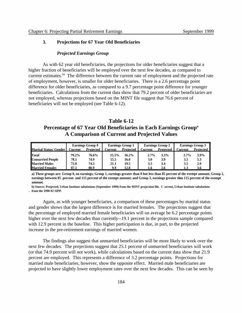
Chapter 6: Projecting Partial Retirement Earnings September 1999
184
Earnings Group 0 Earnings Group 1 Earnings Group 2 Earnings Group 3Marital Status/ Gender Current Projected Current Projected Current Projected Current Projected
Total 79.2% 76.6% 15.5% 16.2% 2.7% 3.3% 2.7% 3.9%Unmarried People 78.1 74.9 15.5 16.0 3.0 3.9 3.5 5.3Married Males 72.0 74.3 21.1 19.5 3.5 3.4 3.5 2.9Married Females 87.1 80.9 9.9 12.8 1.6 2.6 1.3 3.6
a) These groups are: Group 0, no earnings; Group 1, earnings greater than 0 but less than 85 percent of the exempt amount; Group 2, earnings between 85 percent and 115 percent of the exempt amount; and Group 3, earnings greater than 115 percent of the exempt amount.b) Source: Projected, Urban Institute tabulations (September 1999) from the MINT projection file. C urrent, Urban Institute tabulations from the 1990-92 SIPP.
3. Projections for 67 Year Old Beneficiaries
Projected Earnings Group
As with 62 year old beneficiaries, the projections for older beneficiaries suggest that ahigher fraction of beneficiaries will be employed over the next few decades, as compared tocurrent estimates.34 The difference between the current rate of employment and the projected rateof employment, however, is smaller for older beneficiaries. There is a 2.6 percentage pointdifference for older beneficiaries, as compared to a 9.7 percentage point difference for youngerbeneficiaries. Calculations from the current data show that 79.2 percent of older beneficiaries arenot employed, whereas projections based on the MINT file suggest that 76.6 percent ofbeneficiaries will not be employed (see Table 6-12).
Table 6-12Percentage of 67 Year Old Beneficiaries in Each Earnings Groupa
A Comparison of Current and Projected Values
.
Again, as with younger beneficiaries, a comparison of these percentages by marital statusand gender shows that the largest difference is for married females. The projections suggest thatthe percentage of employed married female beneficiaries will on average be 6.2 percentage pointshigher over the next few decades than currently--19.1 percent in the projections sample comparedwith 12.9 percent in the baseline. This higher participation is due, in part, to the projectedincrease in the pre-retirement earnings of married women.
The findings also suggest that unmarried beneficiaries will be more likely to work over thenext few decades. The projections suggest that 25.1 percent of unmarried beneficiaries will work(or that 74.9 percent will not work), while calculations based on the current data show that 21.9percent are employed. This represents a difference of 3.2 percentage points. Projections formarried male beneficiaries, however, show the opposite effect. Married male beneficiaries areprojected to have slightly lower employment rates over the next few decades. This can be seen by

Chapter 6: Projecting Partial Retirement Earnings September 1999
185
Earnings Earnings Earnings Earnings
Cohort Group 0 Group 1 Group 2 Group 3
Total 75.9% 16.9% 3.3% 3.9%
1931-35 78.3 15.1 3.3 3.41936-40 77.1 16.2 3.1 3.51941-45 76.1 17.0 3.3 3.61946-50 75.2 17.5 3.3 3.91951-55 74.8 17.0 4.0 4.21956-60 75.5 17.5 2.8 4.2
a) These groups are: Group 0, no earnings; Group 1, earnings greater than 0 but less than 85 percent of the exempt amount; Group 2, earnings between 85 percent and 115 percent of the exempt amount; and Group 3, earnings greater than 115 percent of the exempt amount.b) Source: Projected, Urban Institute tabulations (April 1999) from the MINT projection file.
the increase in the probability of being in earnings group 0. While 72.0 percent of married malebeneficiaries in the current data were in earnings groups 0, the projections suggest that 74.3percent of married male beneficiaries will be in earnings groups 0. This represents an increase of2.3 percentage points.
A comparison of the current and projected data for the percentage of 67 year oldbeneficiaries in earnings groups 1 through 3 is also presented in Table 6-12. For both unmarriedpersons and married females, the projections show a higher proportion of beneficiaries in earningsgroups 1 through 3. For married male beneficiaries, on the other hand, the projections show alower proportion of beneficiaries in earnings groups 1 through 3, as compared to the current data.
Table 6-13 examines the work behavior of 67 year old beneficiaries by cohort. Lookingdown the six cohort groups reveals a slight decline in the projected fraction of 67 year oldbeneficiaries not working. While 78.4 percent of beneficiaries in the 1931-35 cohort do not work,75.7 percent of beneficiaries in the 1956-60 cohort do not work. The magnitude of the decline inthe fraction of 67 year old beneficiaries not working is significantly smaller than the decline foundfor 62 year old beneficiaries (2.7 percentage points vs. 9.5 percentage points).
Table 6-13Projected Percentage
of 67 Year Old Beneficiaries in Each Earnings Groupa,b
By Cohort

Chapter 6: Projecting Partial Retirement Earnings September 1999
186
Not Working Working
CohortUnmarried
MalesMarried
MalesUnmarried
FemalesMarried Females
Unmarried Males
Married Males
Unmarried Females
Married Females
Total 75.4% 74.3% 74.7% 80.9% 24.6% 25.8% 25.3% 19.1%
1931-35 74.9 72.9 78.7 84.7 25.1 27.1 21.3 15.3
1936-40 78.2 75.8 76.6 83.2 21.8 24.3 23.4 16.9
1941-45 77.0 74.6 73.7 81.4 23.0 25.4 26.3 18.6
1946-50 76.1 74.8 73.6 80.4 23.9 25.2 26.4 19.7
1951-55 75.1 73.0 74.4 79.2 24.9 27.0 25.6 20.9
1956-60 73.1 74.6 73.5 79.5 26.9 25.4 26.5 20.5
a) These groups are: Group 0, no earnings; Group 1, earnings greater than 0 but less than 85 percent of the exempt amount; Group 2, earnings between 85 percent and 115 percent of the exempt amount; and Group 3, earnings greater than 115 percent of the exempt amount.b) Source: Projected, Urban Institute tabulations (September 1999) from the MINT projection file.
Examining beneficiaries by gender shows that females are more likely to not work ascompared to male (see Table 6-14). This differential exists across all six cohort groups, but thedifferential declines from 8.9 percentage points for the 1931-35 cohort to 2.7 percentage pointsfor the 1956-60 cohort.
Table 6-15 further separates beneficiaries by gender and marital status: unmarried males,married males, unmarried females, and married females. While there is some variation across thecohorts, the differences across cohorts for 67 year old beneficiaries are somewhat smaller than thedifferences projected for 62 year old beneficiaries. For example, the difference between the oldestand youngest cohort in the fraction of married female beneficiaries not working is 5.2 percentagepoints for 67 year old beneficiaries, but was double this (10.6 percentage points) for 62 year oldbeneficiaries. This lower degree of variation for 67 year old beneficiaries is consistent with thelower degree of variation in recent earnings and family pension benefits for 67 year oldbeneficiaries, as compared to 62 year old beneficiaries.
Table 6-14Projected Percentage of 67 Year Old Beneficiaries in Each Earnings Groupa,b
By Cohort and Gender

Chapter 6: Projecting Partial Retirement Earnings September 1999
187
Earnings Group 0 Earnings Group 1 Earnings Group 2 Earnings Group 3
Cohort Male Female Male Female Male Female Male Female
Total 74.5% 78.2% 18.6% 14.3% 3.4% 3.2% 3.5% 4.2%
1931-35 73.2 82.1 18.7 12.1 3.8 2.4 4.3 3.41936-40 76.2 80.2 17.4 13.2 3.0 2.9 3.5 3.71941-45 75.1 78.2 18.1 14.3 3.5 3.1 3.3 4.41946-50 75.1 77.5 18.2 14.7 3.0 3.2 3.7 4.71951-55 73.5 77.1 19.5 15.2 3.3 3.6 3.7 4.21956-60 74.2 76.9 19.0 15.1 3.8 3.6 3.0 4.5
Table 6-15Projected Percentage of 67 Year Old Beneficiaries
Who Do Not and Do Work a
by Cohort and Gender/Marital Status
Projected Partial Retirement Earnings
Once individuals are placed into one of the four earnings groups, individuals are assigned alevel of earnings.35 This procedure is more involved for older beneficiaries, as compared to theyounger beneficiaries. This difference is due to the scheduled ad hoc increases, between 1995 and2002, in the Social Security exempt amount for older beneficiaries. These ad hoc adjustmentswere enacted into law in March 1996, and substantially increased the exempt amount for olderbeneficiaries. In the absence of these ad hoc increases, the Social Security exempt amount for 67year old beneficiaries would be roughly $14,500 in the year 2002, while it is scheduled to be$30,000 in the year 2002.36
Table 6-16 presents projected (average) partial retirement earnings for 67 year olds undertwo scenarios: (1) the projection does not take account of the scheduled increase in the exemptamount and (2) the projection does take account of the scheduled increase in the exempt amount.Models estimated with the 1984 SIPP suggest that a $1 increase in the exempt amount willincrease earnings by (1) $0.25 for beneficiaries with earnings well below the exempt amount(group 1), (2) $0.94 for beneficiaries with earnings near or at the exempt amount (group 2), and(3) $1.00 for beneficiaries with earnings over the exempt amount (group 3).37
When the scheduled increases in the exempt amount are not taken into account, projectedpartial retirement earnings are similar to the partial retirement earnings of current beneficiaries. The similarities occur within each of the three earnings groups as well as across the threedemographic groups. This can be seen by comparing columns one and two, columns four andfive, and columns seven and eight. The mean of partial retirement earnings from the projection

Chapter 6: Projecting Partial Retirement Earnings September 1999
188
Earning Group 1 Earning Groups 2 Earning Group 3
Current
Projection Includes Scheduled Increase in
Exempt Amount Current
Projection Includes Scheduled Increase in
Exempt Amount Current
Projection Includes Scheduled Increase in
Exempt Amount Marital Status/ Gender No Yes No Yes No YesTotal 0.156 0.153 0.270 0.435 0.436 0.869 0.887 0.833 1.293Unmarried People 0.158 0.159 0.276 0.433 0.433 0.871 0.798 0.806 1.271Married Males 0.161 0.156 0.272 0.430 0.429 0.853 1.023 0.998 1.444Married Females 0.140 0.142 0.259 0.447 0.449 0.889 0.733 0.739 1.202
Table 6-16Average Partial Retirement Earnings of 67 Year Old Beneficiaries by
Earnings Groupa
A Comparison of Current and Projected Valuesb
that excludes the scheduled increase in the Social Security exempt amount is 0.153 forbeneficiaries in earnings group 1, 0.436 for beneficiaries in earnings group 2, and 0.833 forbeneficiaries in earnings group 3.
When the scheduled increases in the exempt amount are taken into account, projectedpartial retirement earnings are considerably higher. The mean of partial retirement earnings is0.270 for beneficiaries in earnings group 1, 0.869 for beneficiaries in earnings group 2, and 1.293for beneficiaries in earnings group 3. This increase occurs in all three demographic groups thatare shown in Table 6-16 -- unmarried persons, married males, and married females.
The final table examines beneficiaries’ projected earnings by cohort. Because scheduledincreases in the Social Security exempt amount affect later cohorts more than earlier cohorts,primarily the 1931-35 cohort, this table presents projected earnings that both do and do not takeaccount of scheduled increases in the exempt amount. The first column of Table 6-17 presentsprojections of average partial retirement earnings for all 67 year old beneficiaries, which do nottake account of scheduled increases in the exempt amount, and includes those beneficiaries with zero earnings. Average partial retirement earnings do not differ substantially across the sixcohorts, although earnings are projected to be higher for beneficiaries in the younger cohorts ascompared to beneficiaries in the older cohorts. This is consistent with the finding that, in general,a larger fraction of beneficiaries in the younger cohorts will be working than beneficiaries in theolder cohorts. Within earnings groups 1 through 3, projected earnings that exclude scheduledincreases in the exempt amount are similar across cohorts. However, when the scheduled increasein the exempt amount is taken into account there is a large difference between the partialretirement earnings of beneficiaries in the first cohort as compared to later cohorts. This isbecause beneficiaries in the first cohort are least affected by this policy change.

Chapter 6: Projecting Partial Retirement Earnings September 1999
189
Total Earning Group 1 Earning Groups 2 Earning Group 3
Includes Exempt Includes Exempt Includes Exempt Includes Exempt
Amount Increase Amount Increase Amount Increase Amount IncreaseCohort No Yes No Yes No Yes No Yes
Total 0.072 0.123 0.153 0.270 0.436 0.869 0.833 1.293
1931-35 0.067 0.090 0.151 0.207 0.436 0.641 0.842 1.0751936-40 0.065 0.114 0.151 0.275 0.430 0.891 0.812 1.3001941-45 0.071 0.125 0.151 0.275 0.436 0.896 0.824 1.3121946-50 0.075 0.130 0.156 0.276 0.436 0.896 0.840 1.3291951-55 0.074 0.131 0.153 0.276 0.436 0.896 0.835 1.3231956-60 0.074 0.131 0.155 0.279 0.437 0.898 0.839 1.328
a) These groups are: Group 0, no earnings; Group 1, earnings greater than 0 but less than 85 percent of the exempt amount; Group 2, earnings between 85 percent and 115 percent of the exempt amount; and Group 3, earnings greater than 115 percent of the exempt amount.b) Source: Projected, Urban Institute tabulations (September 1999) from the MINT projection file.Current, Urban Institute tabulations from the 1990-92 SIPP.
Table 6-17Projected Partial Retirement Earnings of 67 Year Old Beneficiaries
in each Earning Groupa,b
By Cohort

Chapter 6: Projecting Partial Retirement Earnings September 1999
190
W ( ' $1,1Z % (1,1R % *1,1AvgEarn(35&59) % R1,1AvgEarn(60&64) % >1,1EX % g1,1
E ' b1,2Age % (1,2R % R1,2AvgEarn(60&64) % >1,2EX % 8 % g1,2
APPENDIX A
ESTIMATING MODELS
The discussion in this appendix uses the model for 65-68 year olds as the base case, butreferences are made where the models for 65-68 year olds and 62-63 year olds differ.
Model 1: Probit and Earnings: The first equation in this two-equation modelincorporates the decision to work or not work, and the second is the earnings equation for thoseindividuals who work. The equation for the decision to work is defined below, where the firstsubscript refers to the model number (in this case model 1) and the second subscript refers to theequation number within the model:
Z is a vector of demographic characteristics (including race/ethnicity, educational attainment,gender, marital status, and age), R includes measures of non-labor income available in retirement(401(k), IRA, and Keogh account balances, pension income, and wealth), AvgEarn(35-59) isindividuals' average earnings from age 35 through age 59 (where earnings in each year are dividedby national average earnings), AvgEarn(60-64) is individuals' average earnings from age 60 throughage 64 (divided by national average earnings), and finally, EX is the Social Security exemptamount (which is also divided by national average earnings).38
The second equation in this two-step model is the reduced-form equation for level ofearnings, and it is estimated only on the subset of persons who have nonzero earnings. Thus,earnings for this group of beneficiaries are greater than zero but less than the amount at which theSocial Security benefit is reduced to zero.
The set of explanatory variables is similar to those in the first-stage probit equation, but averageearnings from age 35 to age 59 and most of the demographic variables are omitted. This earningsvariable is excluded from the model because it is unlikely that, for this group of Social Securitybeneficiaries, average earnings from age 35 to 59 adds additional information beyond earnings

Chapter 6: Projecting Partial Retirement Earnings September 1999
191
S ( ' $2,1Z % (2,1R % *2,1AvgEarn(35&59) % R2,1AvgEarn(60&64) % >2,1EX % g2,1
from age 60 to 64.39 Another difference is that this equation includes a sample selection term, . 8This term, referred to the literature as the "inverse mills ratio," takes account of the fact thatworking recipients are different from non-working recipients. In this model, the probit andearnings equation are estimated as a system so the standard errors are efficient.
Model 2: Ordered Probit and Earnings: This model examines factors that influence onwhich segment of the earnings distribution a beneficiary falls. In this specification of the model,beneficiary are in one of four earnings groups: (1) zero earnings, (2) earnings greater than 0 butless than 85 percent of the exempt amount, (3) earnings between 85 percent and 115 percent ofthe exempt amount, and (4) earnings greater than 115 percent of the exempt amount. Theequation for model 2 is very similar to the probit equation estimated under Model 1, and can bewritten as:
The dependent variable S* indicates in which segment of the earnings distribution an individualfalls, and equals 0 if the individual has zero earnings, 1 if the individual has earnings greater than 0but less than 85 percent of the exempt amount, etc. The independent variables are as describedabove under model 1.

Chapter 6: Projecting Partial Retirement Earnings September 1999
192
Probit Earnings RatioExplanatory Variable (obs=1,560) (obs=437)
Non-Hispanic white 0.1297 (0.1053)Education less than 12th grade ** -0.4097 (0.1004) Education equal to 12th grade -0.1355 (0.0887)Male * 0.1830 (0.1010)Married in calender year -0.1233 (0.0810)
Age 63 -0.0722 (0.0718) -0.0220 (0.0524)
Family pension ** -0.0284 (0.0049) -0.0013 (0.0054)Income from assets -0.0071 (0.0048) -0.0001 (0.0027)Balance of 401K, IRA, Keogh 0.0001 (0.0019) -0.0005 (0.0012)
Average past earnings (ages 35-55) -0.1348 (0.1115)Average recent earnings (ages 56-61) ** 0.5486 (0.0905) 0.0660 (0.0903)
Constant ** 0.6862 (0.1367) ** -0.7244 (0.2253)Inverse Mills Ratioa -0.1329 (0.1847)
Pseudo R-squared/R-squaredb 0.066 0.0151Chi-squared / F-statisticc 122.07 (df=11) 1.03 (df= 6, 430)a) The inverse mills ratio is the correction term as described in appendix A.b) Pseudo R-squared calculated for ordered probit and R-squared calculated for earnings equations.c) Chi-squared calculated for the ordered probit and F-statistic calculated for the earnings equations.d) Standard errors in parenthesis.e) Significance at 10 percent is represented by "*".f) Significance at 5 percent is represented by "**".
APPENDIX BPROBIT/EARNINGS MODELS
This appendix presents the results of preliminary probit/earnings models estimated withthe 1990-92 SIPP data. The model results are presented first for 62-63 year old beneficiaries andthen for 65-68 year old beneficiaries.
Table 6-B-1 Probit/Earnings Model
Social Security Beneficiaries Age 62 to 63, 1990-92 SIPP

Chapter 6: Projecting Partial Retirement Earnings September 1999
193
Probit EarningsExplanatory Variable (obs=3,574) (obs=822)
Non-Hispanic white -0.0613 (0.0711)Education less than 12th grade ** -0.3032 (0.0663)Education equal to 12th grade -0.0610 (0.0609)Male ** 0.3330 (0.0655)Married in calender year * -0.1083 (0.0555)
Age 66 -0.0690 (0.0658) 0.0175 (0.0249)Age 67 ** -0.2633 (0.0686) 0.0229 (0.0275)Age 68 ** -0.3120 (0.0698) -0.0333 (0.0277)
Family pension ** -0.0276 (0.0036) ** -0.00306 (0.0015)Income from assets ** -0.0083 (0.0031) 0.0007 (0.0012)Balance of 401K, IRA, Keogh ** 0.0020 (0.0010) * -0.0006 (0.0003)
Average past earnings (ages 35-59) ** -0.3122 (0.0709)Average recent earnings (ages 60-64) ** 0.8761 (0.0613) ** 0.1307 (0.0240)
Constant ** 0.50913 (0.0938) ** -0.3496 (0.4839)Inverse Mills Ratioa -0.0641 (0.0618)
Pseudo R-squared/R-squaredb 0.1051 0.1457Chi-squared / F-statisticc 405.14 (df=13) 7.40 (df= 8, 813)a) The inverse mills ratio is the correction term as described in appendix A.b) Pseudo R-squared calculated for ordered probit and R-squared calculated for earnings equations.c) Chi-squared calculated for the ordered probit and F-statistic calculated for the earnings equations.d) Standard errors in parenthesis.e) Significance at 10 percent is represented by "*".f) Significance at 5 percent is represented by "**".
Table 6-B-2Probit/Earnings Model
Social Security Beneficiaries Age 65 to 68, 1990-92 SIPP

Chapter 6: Projecting Partial Retirement Earnings September 1999
194
APPENDIX CVARIABLES
This appendix presents a brief explanation of the variables included in the models.
Dependent Variables:
Earnings Group: In the ordered probit model, this variable equals 0 if the individual has noearnings, equals 1 if earnings are greater than 0 but less than 85 percent of the exempt amount,equals 2 if earnings are between 85 percent and 115 percent of the exempt amount , and equals 3in earnings are greater than 115 percent of the exempt amount.
Earnings: Ratio of individual earnings to national average earnings.
Explanatory Variables:
Exempt Amount: Ratio of the Social Security exempt amount to national average earnings.
Average Earnings: Earnings, as described above, averaged over the appropriate years.
Family Pension Income: Family (individual and spouse) pension income divided by nationalaverage earnings.
Family Wealth: Family wealth divided by national average earnings.
Family Retirement Account Balances (IRA, 401k, and Keogh): Family account balances dividedby national average earnings.
Age: Dummy variables for age. In the model for 65-68 year olds, the excluded age is 65. In themodel for 62-63 year olds, the excluded age is 62.
Non-Hispanic White: Variable equals 1 if the individual is non-Hispanic white, and equals zerootherwise. Other race/ethnicity categories were considered, but the groups are small -- 86 percentof the sample is non-Hispanic white.

Chapter 6: Projecting Partial Retirement Earnings September 1999
195
Education: Two education variables are included in the models -- education less than high schooland education equals to high school (the excluded category is education greater than high school). Seventy-three percent of the sample members have a high school degree or less.
Male: This variable equals 1 if the individual is male, and equals 0 if the individual is female.
Married: This variables equals 1 if the individual was married during the particular calendar year,and equals zero otherwise.

Chapter 6: Projecting Partial Retirement Earnings September 1999
196
Unmarried People Married Males Married FemalesExplanatory Variable (n=1,831) (n=2,121) (n=2,170)
Education Less than 12th Grade -0.3636 ** (0.0887) -0.2947 ** (0.0661)Education Equal to 12th Grade -0.1082 (0.0843)
Spouse's Age -0.0171 ** (0.0052) -0.0127 (0.0082)
Age 66 -0.1799 * (0.0956)Age 67 -0.2590 ** (0.0941) -0.1800 ** (0.0717) -0.1525 * (0.0882)Age 68 -0.3134 ** (0.0943) -0.3171 ** (0.0729) -0.2771 ** (0.0963)
Family Wealth b -0.0071 (0.0098) -0.0007 (0.0046)Family Pension Benefits -1.2981 ** (0.1838) -0.6591 ** (0.0807) -0.3993 ** (0.0964)Family Retirement Account Balances 0.1461 ** (0.0486) 0.0346 (0.0256)
Average Past Earnings (ages 35-59) -0.1254 (0.0957) -0.5460 ** (0.0769)Average Recent Earnings (ages 60-64) 1.0067 ** (0.0891) 0.7097 ** (0.0531) 1.4283 ** (0.0928) Pseudo R-squared 0.0949 0.0845 0.1292Chi-squared 238.94 (df=10) 278.02 (df=8) 259.03 (df=6)Cutoff value 1 0.5887 (0.1044) -1.0196 (0.3316) 0.3906 (0.5619)Cutoff value 2 1.4245 (0.1108) -0.0222 (0.3315) 1.3291 (0.5641)Cutoff value 3 1.7888 (0.1183) 0.3688 (0.3326) 1.7201 (0.5670)
a These groups are: Group 0, no earnings; Group 1, earnings greater than 0 but less than 85 percent of the exempt amount; Group 2, earnings between 85 percent and 115 percent of the exempt amount; and Group 3, earnings greater than 115 percent of the exempt amount. b Family wealth, family pension benefits, average past earnings, and average recent earnings are divided by national average earnings. c Standard errors in parenthesis.d Significance at 5 percent is represented by "**".e Significance at 10 percent is represented by "*".
APPENDIX DESTIMATION AND PROJECTION RESULTS
THAT INCLUDE RETIREMENT ACCOUNT BALANCES
This appendix presents results of the estimation and projection of partial retirementearnings for beneficiaries when family retirement account balances are taken into account in theanalysis.
Table 6-D-1Ordered Probit Model by Marital Status and Gendera
Social Security Beneficiaries Age 65 to 68, 1990-92 SIPP

Chapter 6: Projecting Partial Retirement Earnings September 1999
197
Marital Status/ Earnings Group 0 Earnings Group 1 Earnings Group 2 Earnings Group 3 Gender Current Projected Current Projected Current Projected Current Projected
Total 79.1% 75.1% 15.5% 16.3% 2.7% 3.3% 2.7% 5.3%Unmarried People 78.1 71.5 15.5 16.0 3.0 3.8 3.5 8.8Married Males 72.0 74.3 21.1 19.5 3.5 3.4 3.5 2.9Married Females 87.1 79.9 10.0 13.2 1.6 2.8 1.3 4.1
Earning Group 1 Earning Groups 2 Earning Group 3
Marital Status/ Current
Projection Includes Scheduled Increase in
Exempt Amount Current
Projection Includes Scheduled Increase in
Exempt Amount Current
Projection Includes Scheduled Increase in
Exempt Amount Gender No Yes No Yes No YesTotal 0.156 0.151 0.268 0.435 0.436 0.871 0.887 0.823 1.288Unmarried People 0.158 0.156 0.273 0.433 0.432 0.871 0.798 0.805 1.275Married Males 0.161 0.156 0.272 0.430 0.429 0.853 1.023 0.998 1.444Married Females 0.140 0.138 0.255 0.447 0.450 0.893 0.733 0.738 1.203
a) This table is based on the ordered probit model presented in Table 6-D-1, which includes family retirement balances. b) These groups are: Group 0, no earnings; Group 1, earnings greater than 0 but less than 85 percent of the exempt amount; Group 2, earnings between 85 percent and 115 percent amount; and Group 3, earnings greater than 115 percent of the exempt of the exempt amount.c) Source: Projected, Urban Institute tabulations (September 1999) from the MINT projection file. Current, Urban Institute tabulations from the 1990-92 SIPP.
Table 6-D-2a
Percentage of 67 Year Old Beneficiaries in Each Earnings Groupb
A Comparison of Current and Projected Valuesc
Table 6-D-3a
Average Partial Retirement Earnings of 67 Year Old Beneficiaries by Earnings Groupa
A Comparison of Current and Projected Valuesb

Chapter 6: Projecting Partial Retirement Earnings September 1999
198
APPENDIX E SIMULATING WORK BEHAVIOR FROM
AGES 63 TO 66 AND AFTER 67
I. OVERVIEW
This appendix describes the method that the MINT model employs for filling in individualearnings between ages 62 and 67 and after age 67. This part of the model combines informationfrom Chapters 2 and 6 with a simple model of the likelihood of remaining in partial retirement. Itcreates a full stream of earnings from age 62 until death for each person who survives to age 62.
When each person in the MINT sample attains age 62, we determine whether he or shehas begun to collect Social Security benefits. If he or she has, then we set his/her earnings level inthat year using the projections from the current chapter. If the person has not yet begun receivingSocial Security, we continue to use the Chapter 2 projection estimates for his/her earnings leveluntil the time of Social Security benefit take-up. When a person starts Social Security benefitreceipt after age 62, he/she receives a starting value for partial retirement earnings at the point oftake-up (if retiring at age 67, this is the exact value for earnings at 67 from earlier in this chapter). Any person who begins receiving her/his benefits before age 67 is then subjected to a probabilityof remaining in the labor force for each age between the age of first receipt and age 66. If theperson’s probability of remaining at work in a given year is higher than a random draw, then he orshe continues to work and receives the same wages as he/she received in the prior year. At age67, nearly all members of the population receive their Chapter 6 earnings projection. After age67, those who are still working are similarly subjected to a probability of remaining at work ineach subsequent year, and they continue to work at their age 67 wage level until they either die orone of their random draws is higher than their stay-at-work probability for that year. Individuals’probabilities of continuing to work are generated by a relatively simple logistic regressionequation which we describe below.
Four separate groups thus receive differential treatment in the process of updatingearnings after age 62. These include: those who begin Social Security receipt at age 62, thosewho begin Social Security receipt between ages 63 and 66, inclusive, those who begin SocialSecurity receipt at age 67, and those who do not collect Social Security. To detail operation ofthe model more clearly, we illustrate the treatment of each of these four groups in turn.

Chapter 6: Projecting Partial Retirement Earnings September 1999
199
1. Person Starts to Receive Social Security at or before age 62
If an individual begins receiving Social Security benefits at or before age 62, we overwritethe Chapter 2 prediction of earnings at age 62 with the partial retirement earnings prediction fromChapter 6. If predicted earnings are positive, we look forward to see if this person will, accordingto the Chapter 6 estimate, still be working at age 67. If so, we then use the person’s predictedprobability of working at age 62 to adjust each of the person’s random draws from age 63 to age66 downward so that each draw will be lower than the probability of staying in partial retirement. We do this in order to promote consistency in work trajectories, so that people will not bejumping into and out of partial retirement each year. If the person is not selected to work at age67, then he/she is exposed to random draws that are adjusted upward. (These two adjustmentsare made in such a way as to preserve the initial uniform distribution from which draws are made). When workers choose, through the random process, to continue to work, their earnings levels arekept constant from the prior year. After age 67, if the person is working at t-1 then he/she isagain exposed annually to a probability of remaining in partial retirement and an independentrandom draw from a uniform distribution determines whether he/she continues working. If he orshe continues to work, he or she does so at the age 67 wage level.
2. Person Starts to Receive Social Security between ages 63 and 66
A person who does not retire until after age 62 retains earnings values from Chapter 2until the year of Social Security retirement. Since people who do not receive Social Security untilafter age 62 are not subjected to the Chapter 6 projections at age 62, we need some kind ofstarting value for their earnings in partial retirement. We use a separate prediction, produced byapplying the algorithm for 62 year-olds from earlier in this chapter to the general populationrather than just the age 62 retiree population, to generate a starting value for these people. Wethen update this projection, using the logistic equations and random draws as above, through age66. If applicable, this process continues at ages 68 and beyond, using the age 67 earnings levelprediction.
3. Start to Receive Social Security at age 67
The starting value for earnings of individuals in this group is simply the Chapter 6prediction at age 67. For each successive year at risk (i.e., each year with nonzero earnings at t-1), a new probability of remaining in partial retirement is calculated and an independent randomdraw is taken. If, on the basis of the random draw, a person chooses to continue to work, thenher/his earnings level at age 67 is maintained.

Chapter 6: Projecting Partial Retirement Earnings September 1999
200
4. Never Receive Social Security
For the small fraction of the population that never receives Social Security, earnings fromChapter 2 are maintained from age 62 through age 67 and earnings are set to zero thereafter.
II. EQUATIONS FOR GENERATING PROBABILITY OF REMAINING IN PARTIAL RETIREMENT
The MINT model of likelihood of remaining in partial retirement is structurally quitesimilar to the Social Security benefit receipt model. It is also a discrete-time, conditionaltransition probability model, and it was estimated from the same data sources. As the precedingdiscussion suggests, in this case the probability we are modeling is the probability that oneremains in partial retirement given that one was engaged in partial retirement (that is, workconcurrent to Social Security benefit receipt) at time t-1. For estimation of this model, person-year observations start at age 63 rather than age 62 (since most people cannot be partially retiredat age 61) and continue much further than in the benefit take-up model, up to age 80.
As in the Social Security benefit take-up model, we use a person-birth year rather than aperson-calendar year as the unit of analysis for estimating model parameters. This implies thatwhile we use MBR data to confirm a person’s Social Security receipt, we use SIPP monthly self-report data on earnings rather than annual (i.e., calendar-year) data from Summary EarningsRecords. Determining whether an individual is a worker or a non-worker in a given birth year ofpartial retirement poses numerous measurement challenges. In a series of alternative tabulations,we found that our estimates are extremely sensitive to whether we use just the birth month or thebirth month and the prior month, or some other combination of lags, in assessing work behavior.
The SIPP estimates suggest that these partial retirees are a special, select group. We didnot identify any significant differences in likelihood of staying in partial retirement across gender,racial, or marital status lines, and thus chose to estimate a single equation rather than separateequations by sex or marital status group for this portion of MINT. The explanatory variables inthe model of partial retirement focus on two major characteristics: one’s taste for work and thereturn that one gets from working. Taste for work is reflected first by the duration of the currentwork spell, that is, the time that has elapsed since one has had a year of zero earnings. A terminteracting age with a dummy variable indicating whether one has less than a high schooleducation reflects the hypthesized increasing lack of desirability of work for the less educated asone ages. Persons with less than a high school education are far more likely to be in positions thatare unrewarding and/or physically demanding, and strains of such jobs are likely to increase withage. A person’s lagged earnings reflects both his or her revealed preference for work and her/hispotential returns from working. An age 65 dummy variable captures a person’s eligibility forMedicare at this age, a factor which greatly diminishes one significant incentive to continued

Chapter 6: Projecting Partial Retirement Earnings September 1999
201
work, the availability of employer-provided health insurance benefits. A person’s wealth profile isreflected in the model through both a home ownership dummy variable and an age-homeownership interaction term.
III. COEFFICIENT ESTIMATES
Table 6-E-1 presents the logistic coefficients from the model estimation phase. We seethat the likelihood of remaining in partial retirement increases with our indicators of attachment tothe labor force and returns to working, as evidenced by the positive signs on coefficients forduration of work spell and level of lagged earnings, and decreases when work incentives decline,as evidenced by the negative sign on the coefficient for the age 65 dummy variable. Past earningstend to depress the likelihood of continuing to work, with higher earnings from both ages 35 to55 and ages 56 to 61 suggesting a lesser likelihood of additional work, though these relationshipsare not statistically significant. While wealth, as evidenced here through homeownership, actuallyincreases the likelihood of staying at work, this effect declines with age. For those with very littleeducation (less than a high school degree), the likelihood of working declines with age.
Table 6-E-1 Logistic regression coefficients: Remain in Partial Retirement
Variable
Parameter Estimate(Standard Error)N=3317 person years
Intercept 0.4324** (0.1019)
Age 65 -0.2457** (0.1299)
Duration of current work spell 0.0205** (0.00275)
Age*Education < 12 -0.00341** (0.00127)
Age*Homeowner -0.0255* (0.0124)
Homeowner? 2.0373* (0.8559)
Earnings ages 35-55 -0.1531 (0.1169)
Earnings ages 56-61 -0.1519 (0.0950)
Earnings at t-1 0.1930* (0.0836)
* indicates p<.05; ** indicates p<.01
Source: Urban Institute estimates, September, 1999

Chapter 6: Projecting Partial Retirement Earnings September 1999
202
IV. RESULTS FROM SIMULATION ANALYSES
When we apply these coefficients annually to the members of the MINT sample who arepartially retired, we find that average probabilities of remaining in partial retirement are around0.63 in the first years of retirement, between ages 62 and 64, decline to 0.57 at age 65, but thenlevel off to a rate of around 0.60 at later ages. Figure 6-E-1 contrasts MINT generatedprobabilities to remain in work after age 62 and the work rates that these probabilities imply. While the average probabilities that MINT generates are roughly consistent with estimates fromother sources, the work rates are systematically lower in MINT, even for workers in oldercohorts, than are found in data sets like SIPP and CPS. While fractions of U.S. residents in thelabor force after age 75 are indeed small, less than one in twenty according to recent (1996) U.S.Census Bureau estimates, they are nontrivial, and MINT clearly understates them.
There are several reasons for the discrepancy between MINT and other sources. First,because the MINT model assumes full retirement (for Social Security purposes) at age 67, andthus earnings levels within a fairly constrained range for older workers, this portion of the modelgenerates an unrealistically low proportion of the population in the labor force at ages greaterthan 67. Recall from Table 6-E-1 that lagged earnings are a major predictor of subsequent work. If lagged earnings cannot go above 1.5 times the Social Security exempt amount, thenprobabilities of staying at work will be too low at several critical points. The fact that the modeldoes not currently allow re-entry into employment after age 67 further exacerbates this problem.
It is also important to note that beyond age 70 the earnings of Social Security recipientsare no longer subject to the retirement test, so individuals no longer have an incentive to keepearnings at or below the exempt amount. MINT does not at this time take this policy intoaccount. While few individuals are affected by this change, this shift could greatly impact theaggregate amount of earnings income generated in the model.
In general, then, additional development of this portion of the model could address theseshortcomings, and help to calibrate its estimates more closely to external benchmarks. Greatercalibration of this portion of MINT could make it a valuable tool for examining this small butinteresting group of working Social Security recipients.

Chapter 6: Projecting Partial Retirement Earnings September 1999
203
0
0.1
0.2
0.3
0.4
0.5
0.6
0.7
62 64 66 68 70 72 74 76 78
Age
Rat
e/P
rob
abili
ty
MINT Work Rate
MINT Probability toStay at Work
Figure 6-E-1Age Patterns in Work at and after Age 62
Source: Urban Institute tabulation, September, 1999

Chapter 6: Projecting Partial Retirement Earnings September 1999
204
CHAPTER 6: REFERENCES
Burtless, Gary and Robert A. Moffitt. 1984. “The Effect of Social Security Benefits on the LaborSupply of the Aged,” in Henry J. Aaron and Gary Burtless, eds. Retirement and EconomicBehavior. Washington DC: The Brookings Institution.
Social Security Administration, Office of Research, Evaluation and Statistics. 1997. AnnualStatistical Supplement, 1997 to the Social Security Bulletin. Washington, DC: Author.
U.S. Bureau of the Census. 1996. Employment status of the civilian noninstitutional populationby age, sex, and race for 1996. Obtained via website, URL:http://ferret.bls.census/gov/macro/171996/empearn/3_000.htm.
Table 6-1Ordered Probit Model
167
Table 6-2
Social Security Beneficiaries Age 65 to 68, 1990-92 SIPP 170
Probit/Earnings ModelPersons Age 65 to 68, SIPP 1984
Table 6-4Ordered Probit Model
175
Table 6-5
Social Security Beneficiaries Age 65 to 68, 1984 SIPP 177
Percentage of 62 Year Old Beneficiaries in Each Earnings GroupA Comparison of Current and Projected Values
Table 6-7Projected Percentage of 62 Year Old Beneficiaries in Each
180

Chapter 6: Projecting Partial Retirement Earnings September 1999
205
Table 6-8Projected Percentage of 62 Year Old Beneficiaries in Each Earnings Group By Cohort and Gender 180
Table 6-9Projected Percentage of 62 Year Old Beneficiaries Who Do and Do Not WorkBy Cohort and Gender/Marital Status 181
Table 6-10Partial Retirement Earnings of 62 Year Old Beneficiaries in Each Earnings GroupA Comparison of Current and Projected Values 181
Table 6-11Projected Partial Retirement Earnings of 62 YearOld Beneficiaries in Each Earnings Group By Cohort 183
Table 6-12Percentage of 67 Year Old Beneficiaries in Each Earnings GroupA Comparison of Current and Projected Values 184
Table 6-13Projected Percentage of 67 Year Old Beneficiaries in Each EarningsGroup By Cohort 185
Table 6-14Projected Percentage of 67 Year Old Beneficiaries in Each Earnings GroupBy Cohort and Gender 186
Table 6-15Projected Percentage of 67 Year Old Beneficiaries Who Do Not and DoWork by Cohort and Gender/Marital Status 187
Table 6-16Average Partial Retirement Earnings of 67 Year Old Beneficiaries byEarnings Group A Comparison of Current and Projected Values 188
Table 6-17Projected Partial Retirement Earnings of 67 Year Old Beneficiaries in each Earning Group By Cohort 189
Table 6-B-1 Probit/Earnings Model Social Security Beneficiaries Age 62 to 63, 1990-92 SIPP 192
Table 6-B-2Probit/Earnings ModelSocial Security Beneficiaries Age 65 to 68, 1990-92 SIPP 193

Chapter 6: Projecting Partial Retirement Earnings September 1999
206
1. The normal retirement age is currently 65 years old but is scheduled to increase to 67 by theyear 2022.
2. Individuals from the 1990 SIPP panel were born between 1926 and 1928, individuals fromthe 1991 panel were born between 1927 and 1929, and individuals from the 1992 panel were bornbetween 1928 and 1931.
3. For example, beneficiaries who were 62 years old in 1990 and 63 year olds in 1991 wereincluded in the sample twice.
Table 6-D-1Ordered Probit Model by Marital Status and GenderSocial Security Beneficiaries Age 65 to 68, 1990-92 SIPP 196
Table 6-D-2 Percentage of 67 Year Old Beneficiaries in Each Earnings GroupA Comparison of Current and Projected Valuesc 197
Table 6-D-3 Average Partial Retirement Earnings of 67 Year Old Beneficiariesby Earnings Group A Comparison of Current and Projected Values 197
Table 6-E-1 Logistic regression coefficients: Remain in Partial Retirement
201
CHAPTER 6: LIST OF FIGURES
Figure 6-1 Ratio of Earnings to Exempt Amount Persons Age 65 to 68, SIPP 1984 161
Figure 6-2Ratio of Earnings to Exempt Amount Persons Age 65 to 68, SIPP 1990-92 162
Figure 6-3Ratio of Earnings to Exempt Amount Persons Age 62 to 63, SIPP 1990-92 163
Figure 6-E-1Age Patterns in Work at and after Age 62 203
CHAPTER 6: ENDNOTES

Chapter 6: Projecting Partial Retirement Earnings September 1999
207
4. Allowing an individual to enter the sample more than once implicitly assumes that theirbehavior in one year is independent of their behavior in the next year. While independence acrosstime may not hold, models estimated for older beneficiaries (age 65-68) suggest that includingbeneficiaries in the sample multiple times has little effect on the estimated coefficients (see below).
5. An individual is identified as working if they have covered earnings, as recorded on the SERdata file.
6. The sample of older beneficiaries (65-68 year olds) is significantly larger than the sample foryounger beneficiaries, so we estimated models on a sample of unique individuals as well as on asample where individuals are included multiple times. The estimated coefficients from these twomodels were similar.
7. Individuals from the 1990 SIPP panel were born between 1921 and 1925, individuals fromthe 1991 panel were born between 1922 and 1926, and individuals from the 1992 panel were bornbetween 1923 and 1928.
8. In the 20 years prior to 1995, the 1977-83 period is the only one in which there was anexogenous (or "ad hoc") increase in the exempt amount (relative to the average wage) for personsage 65 through 68. Also, during this time, there was no exogenous increase in the exemptamount (relative to the average wage) for persons age 62 through 64.
9. This is because the design requires us to use the 1984 SIPP to look "back" at individuals'behavior between 1977 through 1983.
10. Burtless and Moffitt (1984) p. 156.
11. The samples are: 65-68 year olds with the 1984 SIPP, 65-68 year olds with the 1990-92SIPP, and 62-63 year olds with the 1990-92 SIPP.
12. See Appendix 6-A for details of the probit/earnings model.
13. These models were estimated with the 1990-92 SIPP and are presented in Appendix 6-B,Tables B-6-1 and B-6-2.
14. See Appendix 6-A for details of the ordered probit model.
15. The earnings are assigned in a way that allows us to incorporate the effect of the scheduledincreases in the Social Security exempt amount on beneficiaries' earnings. This procedure isdescribed in more detail in the next section.

Chapter 6: Projecting Partial Retirement Earnings September 1999
208
16. This approach is valid because the Social Security exempt amount is orthogonal to the otherexplanatory variables in the model (i.e., the individuals' demographic and economiccharacteristics).
17. The first earnings equation includes all persons with earnings greater than 0 but less than 85percent of the exempt amount, the second earnings equation includes persons with earningsbetween 85 percent and 115 percent of the exempt amount, and the third earnings equationincludes persons with earnings greater than 115 percent of the exempt amount.
18. See Appendix 6-C for details about these explanatory variables.
19. Average earnings are calculated starting at age 45 in the sample from the 1984 SIPPbecause it is the first age at which earnings is available for the entire sample (since the earliest yearof earnings is 1951).
20. Marital status is excluded from the analysis of the 1984 SIPP because this variable is missingfor roughly 50 percent of sample. This large percentage of missing data is due to the fact that themarital history questions were asked at the end of the survey period. Note that the model resultswere altered only minimally when this variable was included.
21. Only the more recent measure of average earnings is included in the earnings equationbecause it is unlikely that, for this group of Social Security beneficiaries, average earnings fromthe more distant past adds additional information beyond recent earnings.
22. The pseudo-R-squared is defined as (1 - Lu/Lr), where (1) "Lu" is the log-likelihood valueof the "unrestricted" model and (2) "Lr" is the log-likelihood value of the "restricted" model. Theratio of the unrestricted log-likelihood and restricted log-likelihood (Lu/Lr) is between zero andone, so the pseudo-R-squared also falls between zero and one.
23. Of the 6,138 beneficiaries, 4,912 are in earnings group 0, 912 in earnings group 1, 156 inearnings group 2, and 158 in earnings group 3.
24. While the final projections exclude the effects of family retirement account (401(k), IRA,and Keogh) balances, Table 6-D-2 in Appendix 6-D presents the projections based on thecoefficients that include family account balances.
25. The P-value for the estimated coefficients are 0.44 to 0.91, respectively. Also note thatfamily retirement account balances is excluded because the P-value is very high at 0.94.
26. The P-values range from 0.73 to 0.93.
27. An extension of this approach would be to estimate different effects by gender and maritalstatus.

Chapter 6: Projecting Partial Retirement Earnings September 1999
209
28. The model results with regard to the other variables in the model suggest that (1) non-Hispanic whites are less likely to work, (2) persons with less than a high school education are lesslikely to work, (3) males are more likely to work, (4) older persons are less likely to work, and (5)higher average earnings between the ages of 60 and 64 increases the probability of working, whilehigher average earnings between the ages of 45 and 59 decrease the probability of working.
29. Subsequent refinements of the model should, however, incorporate revised definitions of theearnings groups. Further tests of beneficiaries' responses to increases in the Social Securityexempt amount suggest that our estimates may be biased upwards. Our additional work suggeststhat the regression coefficient is about 0.06 (rather than 0.25) for beneficiaries in group 1 and0.80 (rather than 0.94) for beneficiaries in group 2. It is unlikely, however, that this will have thesignificant effect on the overall MINT results.
30. Earnings are measured as the ratio of nominal earnings to national average earnings.
31. The weights available in 1990-92 SIPP panels are taken into account with this procedure.
32. These percentages and all other percentages presented below are based on weighted data.
33. Individuals in 1931-35 cohort are age 62 between 1993 and 1997, while individuals in the1956-60 cohort are age 62 between 2018 and 2022.
34. As is the case for younger beneficiaries, the current rates of employment are based oncalculations from the 1990-92 SIPP.
35. As with younger beneficiaries, earnings are measured relative to national average earning.
36. This estimate of $14,500 is based on the expected increase in the exempt amount foryounger beneficiaries (i.e., persons under the normal retirement age) to the year 2002.
37. The estimated coefficient on the exempt amount for earnings group 3 is 1.44, but we use1.00 in the projection because (1) we cannot reject the null hypothesis that this coefficient is equalto 1.0 and (2) we do not expect this coefficient to be higher than 1.0.
38. The model for 62-63 year olds is similar except that (1) earnings are average from age 35 toage 55 for the first earnings measure and from age 56 to age 61 for the second earnings measureand (2) the exempt amount is excluded from the model (since there is no variation in the exemptamount for this group).
39. For 62-63 year old beneficiaries, average earnings from age 35 to age 55 is excluded fromthe earnings equation.

210
CHAPTER 7
PROJECTING RETIREMENT INCOMES TO 2020
I. OVERVIEW
This chapter brings together all components of income and assets at the age of initial SocialSecurity receipt. It then projects total annual family income for all remaining years of life, for everyperson on the merged SIPP-SER files in the 1931-1960 birth cohorts, through the year 2020. Theprojection of total family income allows us to estimate family well-being of Social Security recipientsborn between 1931 and 1960 from 1997 through the year 2020.
The predictions of income and assets from early retirement until death use as inputs the resultsof previous chapters in this report and the demographic projections by RAND. They use RAND’sdemographic projections to determine marital status and mortality. They use the earnings projectionsfrom Chapter 2 to determine Adjusted Indexed Monthly Earnings (AIME) and Social Securitybenefits. They use the projections of income at retirement from defined benefit (DB) plans andcharacteristics of DB plans from Chapter 3 to project DB plan income, including any cost-of-livingadjustments, throughout retirement. They use the projections of defined contribution (DC) pensionbalances and IRA balances from Chapter 3 and the projections of housing and other financial wealthreported in Chapter 4 to determine initial stocks of housing wealth and “non-annuitized” financialwealth at retirement. They use the starting age of Social Security benefits from Chapter 5 todetermine the date of retirement and the projection of partial retirement earnings from Chapter 6 todetermine income from earnings of Social Security beneficiaries.
The inputs from earlier chapters, combined with an assumption that housing wealth remainsconstant in real terms, gives us the path in retirement of all sources of income except income fromnon-annuitized financial assets. To obtain the latter, we need to know the rate at which the stock ofthese assets changes in retirement, which depends on the decisions of individuals and couples on howmuch to consume and how much to save. We project changes in the stock of post-retirementfinancial wealth using a reduced-form model of the rate of decline of financial assets with age forolder Americans. This model is estimated from a synthetic panel consisting of multiple panels (1984and 1990-93) of Survey of Income and Program Participation (SIPP) data merged with earnings datafrom the Summary Earnings Records (SER) and Social Security entitlement and mortality data fromthe Master Beneficiary Records (MBR). Finally, we convert the stock of financial assets into incomeby calculating the annuity the individual or couple could purchase from 80 percent of these assets.This model allows families to save from their income or borrow from their assets.

Chapter 7: Projecting Retirement Incomes to 2020 September 1999
211
The projections we report show that unmarried individuals and nonwhites are becoming anincreasing proportion of the aged population. Because these groups have a relatively high incidenceof poverty, we estimate that poverty rates among the aged will increase. We find that the povertyrate of later cohorts is higher than the poverty rate of earlier cohorts, and that per capita income isbecoming less evenly distributed over time. About 10 percent of the youngest Social Securitybeneficiaries will be in poverty in the year 2020, compared to about 8 percent of similarly aged SocialSecurity beneficiaries in 1990. High school dropouts and individuals who never marry areincreasingly in poverty in retirement in 2020 compared to 1990.
The organization of this chapter is as follows. In section II, we summarize our statisticalestimates of the changes in financial assets as people age and describe the data we used in theestimation. In section III, we describe our methodology for decaying income from assets over timeand our methodology for calculating family income in retirement. In section IV, we describe thechange in the composition of initial Social Security recipients by cohort. We focus on thecompositional changes by cohort that are important for our model of the decay of financial assets inretirement. We then describe family income of Social Security beneficiaries at first benefit receipt.We do this separately for husbands, wives, and single individuals, and then for all individuals on a percapita basis. Then we describe the distribution of income by gender and cohort. In section V, wefirst describe the characteristics of our projection sample in the year 2020 and show their projectedincome as a percent of poverty. Next, we describe the changes in poverty rates among the aged inthe year 2020. We then compare characteristics and income of the 1990 aged population with the2020 aged population. Finally, in section VI, we present our conclusions.
II. ESTIMATES OF POST-RETIREMENT CHANGES IN FINANCIALASSETS WITH AGE
We estimated a reduced-form model of the rate of decline of financial assets for olderAmericans. These estimates are based on a cohort analysis of multiple panels of Survey of Incomeand Program Participation (SIPP) data merged with earnings data from the Summary EarningsRecords (SER) and Social Security entitlement and mortality data from the Master BeneficiaryRecords (MBR).
1. Description of the Estimating Equation
The rate of decline of financial assets for aged families is represented as a function ofdemographic variables, birth cohort, past earnings, current Social Security benefit and DB pensionincome, and mortality. The equation estimates the curvature of the age-wealth profile for variouspopulation subgroups and should capture the rate of saving or dissaving of retired individuals as theyage. The form of the equation is as follows:
Ln(W) = $0 + $1X +$2Y(age) + ,

Chapter 7: Projecting Retirement Incomes to 2020 September 1999
212
where, W is financial assets, Ln is the natural logarithmic transformation, $0 is an intercept term, Xis a vector of covariates expected to influence financial wealth, Y is a vector of covariates interactedwith age, the $is are parameters to be estimated, and , is a random error term.
The X vector includes the following explanatory variables: family Social Security benefit, DBpension income, average indexed annual earnings from age 50 to age 60, gender, marital status, race,educational attainment, natural logarithm of home equity for homeowners, an indicator for the last27 months of life, and birth cohort. The Y vector includes interaction terms (slope parameters)between age and dummy variables for race, homeownership, presence of a high earner in thehousehold, defined benefit pension coverage indicator, and widowhood. In all cases, we expressincome and wealth as a percentage of the economy-wide average wage. While other characteristicsmight also explain changes in financial wealth in old age, we are limited to those variables availablein the MINT model. Therefore, we cannot include explanatory variables such as health status, healthinsurance coverage, living arrangement, farm ownership, or business ownership, among others in ourmodel.1
Individuals differ greatly in both their ability to accumulate assets into retirement and theirwillingness to spend them post-retirement. The estimates in this section reflect this heterogeneity.
Our model allows families to increase or reduce their financial wealth in retirement. Figures7-1 and 7-2 illustrate two different patterns of wealth change. Figure 7-1 displays the amount andcomposition of total wealth for a man expected to live until age 83, who might be characterized asa “financial asset saver” because he consumes less than his income from financial assets. (He stillconsumes more than his total economic income because the bulk of his total wealth is in the form ofannuitized assets, which permits him to consume from principal as well as income.) Ignoring theimpact of cost-of-living adjustments, he gets an annual Social Security benefit of 30 percent of theeconomy-wide average wage, a defined benefit pension of 40 percent of the average wage, andemployment earnings at age 65 to age 67 of 50 percent of the average wage. The remainder of hiswealth is in other financial assets. At age 65, this amounts to three times the average wage. Eachyear he can consume from his total wealth. Since he is a saver, even though his total wealth isdeclining, the value of his financial assets (deflated by the average wage) increases. In contrast,Figure 7-2 displays the amount and composition of wealth for a man with the same initial wealth andlife expectancy, who might be characterized as a “permanent income dissaver” because he consumesmore than his permanent income. His other financial assets are essentially depleted by age 75, andhe lives his surviving days on his Social Security benefit and defined benefit pension.

Chapter 7: Projecting Retirement Incomes to 2020 September 1999
213
Figure 7-1Amount and Composition of Wealth by Age
Financial Asset Saver
0
2
4
6
8
1 0
1 2
6 5 6 7 6 9 7 1 7 3 7 5 7 7 7 9 8 1 8 3
A g e
Wea
lth/
Ave
rage
Wag
e
O ther Financia l Asse ts
Earnings
D B P e n s ion
S o c ia l Secur ity
Figure 7-2Amount and Compostion of Wealth by Age
Permanent Income Dissaver
0
2
4
6
8
1 0
1 2
6 5 6 7 6 9 7 1 7 3 7 5 7 7 7 9 8 1 8 3
A g e
Wea
lth/
Ave
rage
Wag
e
O ther F inancia l Asse t s
Earn ings
D B P e n s ion
S o c ia l Secu r ity

Chapter 7: Projecting Retirement Incomes to 2020 September 1999
214
2. Data
We constructed a sample of families from the 1984, 1990, 1991, 1992 and 1993 SIPP panelsincluding the pension and wealth topical module information. From the SIPP, we obtain demographicdata including age, gender, marital status, educational attainment, race, and birth date. The SIPP alsoreports DB pension incomes from private payers, state and local government, the military, and otherfederal government. From the pension plan coverage topical modules, we obtain IRA, Keogh, and401(k) balances, information on joint and survivor pension participation, and an indicator for whetherpensions receive a cost-of-living adjustment.2 The wealth topical modules report home, vehicle, otherreal estate, and farm and business equity (value - debt). The SIPP also shows stock, mutual fund, andbond values, checking, saving, money market, and certificate of deposit account balances, andunsecured debt (credit card and doctor bills).
Our measure of financial assets is the sum of family IRA, Keogh, and 401(k) balances; vehicle,other real estate, and farm and business equity (value - debt); stock, mutual fund, and bond values;checking, saving, money market, and certificate of deposit account balances, less unsecured debt.For simplicity, we call this sum “financial assets,” but it really represents a more general definition ofwealth.
The Bureau of the Census matched each of these SIPP panels to the Social SecurityAdministration Summary Earnings Records (SER) and the Social Security Administration MasterBeneficiary Records (MBR). The SER has information on Social Security covered earnings and thenumber of covered quarters per year from 1951 to 1996. The MBR contains the Social Securitymonthly benefit amount (MBA), primary insurance amount (PIA), and type of benefit paid, for threedifferent periods. The three different periods vary by SIPP panel. Table 7-1 shows the dates that theMBR records cover by SIPP panel. For 62-year-olds in 1984, we can observe their Social Securitybenefit even if they don’t start receiving it until age 73. It also has the date of current entitlement,date of initial entitlement, date of birth, and date of death. For beneficiaries who die, the MBA is setto zero, but the PIA is left intact. For beneficiaries who die after the SIPP survey but before the firstMBR observation, we calculate the MBA from the PIA. Individuals who never receive a SocialSecurity benefit do not have an MBR record. This includes uncovered workers and individuals whoare below the retirement age and not collecting disability or survivors’ benefits.
Social Security income is included as an explanatory variable in our model of post-retirementfinancial assets. At the time of the SIPP survey, however, some of the individuals in our sample arenot receiving Social Security yet. Their Social Security wealth, however, influences both theiraccumulation and rate of decay of these assets. For individuals not

Chapter 7: Projecting Retirement Incomes to 2020 September 1999
215
Table 7-1Date of Master Beneficiary Record Information by SIPP Panel
SIPP Panel First MBR Date Second MBR Date Third MBR Date
1984 1991 1992 1995
1990 1991 1992 1995
1991 1992 1993 1995
1992 1993 1994 1998
1993 1994 1995 1998
Source: Social Security Administration.
receiving Social Security benefits at the SIPP interview, but who will receive Social Security in thefuture, we assign their Social Security income to be their future Social Security income discountedfor the number of years until they begin to receive Social Security. This effectively turns SocialSecurity income in the regression into a measure of price adjusted lifetime earnings.
Consistent with other tasks in the MINT project, we measure financial wealth in any year byits value relative to the average annual wage of Social Security covered employees in that year.Consequently, changes in wealth are measured relative to changes in the average wage. For example,if the average wage increases by two percent per year and nominal wealth increases by one percentper year over the same period, our measure would show wealth declining by approximately onepercent per year.
Table 7-2 compares growth rates in the average wage and in the price level, as measured bythe CPI-U, over years spanning the estimation period (1983-93) and the projection period (1997-2020). In most 5-year periods, wages grew (and are projected to grow) faster than prices -- that is,the real wage was increasing, although for two of the 5-year periods (1980-84 and 1990-94), realwages declined slightly. Because wages are rising slightly faster than prices throughout the projectionperiod (by almost one percent per year after 2010), real wealth will decline slightly less, or increaseslightly more, than our measure of wealth (which is a multiple of the average wage).
We limited our sample to families that include individuals born in or before 1922. For marriedcouples, we retained all the information about the spouse regardless of his or her age. For the 1984panel, individuals born in 1922 were 62 years old. In the 1990 panel, individuals born in 1922 were68 years old. By the 1993 panel, they were 71 years old. Combining the SIPP panels in this fashioncreates a synthetic panel. While we do not follow specific individuals over time, we can observe thecharacteristics and wealth of samples of the aged as they age.
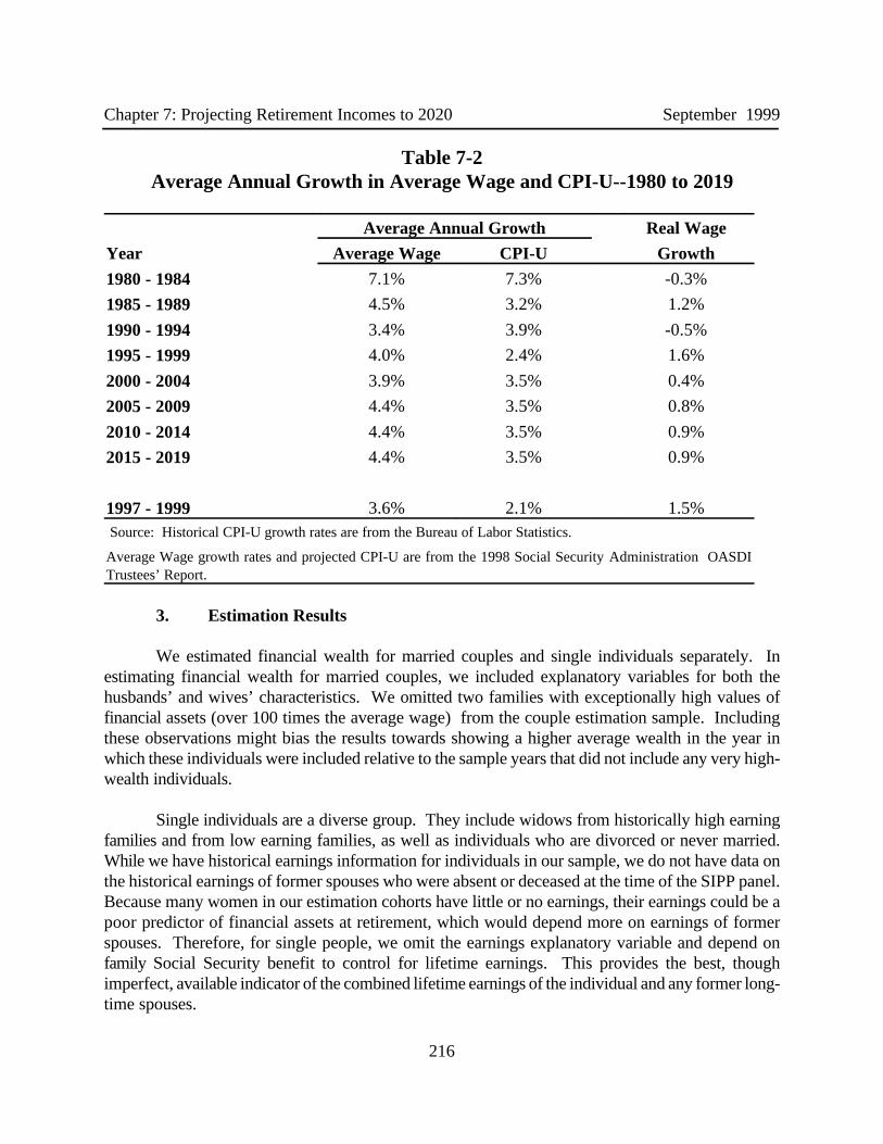
Chapter 7: Projecting Retirement Incomes to 2020 September 1999
216
Table 7-2Average Annual Growth in Average Wage and CPI-U--1980 to 2019
Average Annual Growth Real Wage
Year Average Wage CPI-U Growth
1980 - 1984 7.1% 7.3% -0.3%
1985 - 1989 4.5% 3.2% 1.2%
1990 - 1994 3.4% 3.9% -0.5%
1995 - 1999 4.0% 2.4% 1.6%
2000 - 2004 3.9% 3.5% 0.4%
2005 - 2009 4.4% 3.5% 0.8%
2010 - 2014 4.4% 3.5% 0.9%
2015 - 2019 4.4% 3.5% 0.9%
1997 - 1999 3.6% 2.1% 1.5% Source: Historical CPI-U growth rates are from the Bureau of Labor Statistics.
Average Wage growth rates and projected CPI-U are from the 1998 Social Security Administration OASDITrustees’ Report.
3. Estimation Results
We estimated financial wealth for married couples and single individuals separately. Inestimating financial wealth for married couples, we included explanatory variables for both thehusbands’ and wives’ characteristics. We omitted two families with exceptionally high values offinancial assets (over 100 times the average wage) from the couple estimation sample. Includingthese observations might bias the results towards showing a higher average wealth in the year inwhich these individuals were included relative to the sample years that did not include any very high-wealth individuals.
Single individuals are a diverse group. They include widows from historically high earningfamilies and from low earning families, as well as individuals who are divorced or never married.While we have historical earnings information for individuals in our sample, we do not have data onthe historical earnings of former spouses who were absent or deceased at the time of the SIPP panel.Because many women in our estimation cohorts have little or no earnings, their earnings could be apoor predictor of financial assets at retirement, which would depend more on earnings of formerspouses. Therefore, for single people, we omit the earnings explanatory variable and depend onfamily Social Security benefit to control for lifetime earnings. This provides the best, thoughimperfect, available indicator of the combined lifetime earnings of the individual and any former long-time spouses.

Chapter 7: Projecting Retirement Incomes to 2020 September 1999
217
The regression results are displayed in Table 7-3. For married couples, other financial wealthis positively correlated with increased Social Security benefit, home value, pension income, andaverage indexed earnings between ages 50 and 60. The husband’s level of education is positivelyrelated to wealth. For the husband, completion of a high school education increases estimatedfinancial wealth by about 44 percent and completion of a college education increases estimatedfinancial wealth by about 66 percent, compared to high school dropouts (the omitted educationcategory in the regressions). The return for women’s education is not as large as for men’seducation, but it is still positive. Compared with high school dropouts, wives’ completion of a highschool education increases the couple’s estimated financial wealth by about 43 percent and theircompletion of a college education increases estimated financial wealth by about 45 percent.
Age of initial Social Security entitlement increases the estimated value of other financialwealth. Most families that postpone retirement continue to work and presumably also save.Postponing retirement also increases the Social Security benefit, both due to the effect of the actuarialreduction for early retirement and to the inclusion of a potentially higher level of earnings in theAIME calculation. For a husband, estimated other financial assets increase one percent for every yearhe waits to collect Social Security. For a wife, estimated other financial assets increase about twopercent for every year she waits to collect Social Security.
Financial assets vary among cohorts, but in a complicated way. The first earnings observationwe have for any individual is 1951. Therefore, we have fewer earnings observations for each earlierbirth cohort. For earlier birth cohorts, the 1951 earnings are for late in the career, and thereforehigher on average. These high earnings were subject to a lower taxable maximum, because thetaxable maximum was considerably lower in the 1950s than in the 1980s (see Figure 7-3). SocialSecurity beneficiaries first entitled after 1978 (born before 1917) were based on an average monthlywage calculation (AMW). Beginning in 1979, the formula for calculating Social Security benefits waschanged to be based on the average indexed monthly earnings (AIME). This effectively reduced theSocial Security entitlement for those born in 1917 or later. As a political gesture, Congress phasedin the effect of the AMW to AIME switch for individuals first entitled to Social Security between1979 and 1983 (born between 1917 and 1921).
We included cohort identifiers in the model to control for these complex changes. Our resultsshow that husbands born between 1906 and 1910 have about 11 percent lower estimated financialassets compared to husbands born before 1906. Husbands born between 1911 and 1916 have 29percent lower estimated financial assets compared to husbands born before 1906, and those born after1917 have 44 percent lower estimated financial assets. These figures indicate the expected wealthin any cohort, controlling for fixed amounts of other independent variables. While not all of thecohort parameter estimates are individually statistically significant at the 95 percent confidence level,the group of cohort parameters estimates is statistically significant.One reason that later cohorts have lower wealth, relative to the other predictors is that they havehigher covered earnings than earlier cohorts, reflecting increased Social Security taxes and

Chapter 7: Projecting Retirement Incomes to 2020 September 1999
218
Table 7-3OLS Regression Results by Marital Status for Dependent Variable Log
Financial Assets
Couples Singles
Variable ParameterEstimate
StandardError
ParameterEstimate
Standard Error
Intercept terms
Intercept -2.523 0.772 -1.790 0.516
Social Security benefit 1.130 0.184 2.524 0.203
Log of home wealth 0.405 0.033 0.342 0.032
Head DB pension 0.726 0.094 1.374 0.117
Wife DB pension 0.376 0.228 . .
Head average earn age 50 to 60 0.400 0.073 . .
Wife average earn age 50 to 60 0.026 0.079 . .
Male . . 0.063 0.062
Divorced . . -0.366 0.103
Widow . . 1.924 0.585
Black . . -0.904 0.220
Hispanic . . -0.317 0.189
Head high school 0.438 0.064 0.498 0.053
Wife high school 0.426 0.063 . .
Head college 0.658 0.099 0.937 0.096
Wife college 0.450 0.119 . .
Head age initial entitlement 0.011 0.010 0.016 0.007
Wife age initial entitlement 0.019 0.007 . .
1906<=head born<=1910 -0.106 0.121 -0.277 0.082
1911<=head born<=1916 -0.290 0.111 -0.405 0.085
1917<=head born+ -0.437 0.115 -0.588 0.102
Head or wife dies within 27 months -0.207 0.079 -0.256 0.085
Slope terms
Head age by homeowner -0.019 0.003 -0.016 0.002
Head age by black -0.004 0.003 . .
Head age by white 0.009 0.002 0.007 0.003
Head age by family get pension -0.003 0.001 . .
Head age by high earnings 0.004 0.001
Head age by widowed -0.027 0.008
Source: The Urban Institute tabulations of the SIPP merged with SER and MBRdata.
Notes: Bolded parameter estimates are statistically significant at the 5 percent level.

Chapter 7: Projecting Retirement Incomes to 2020 September 1999
219
0
20
40
60
80
100
120
1950 1955 1960 1965 1970 1975 1980 1985 1990
Year
Per
cent
Men Women
Source: Social Security Administration Annual Statistical Supplement 1998.
Figure 7-3Percent of Workers With Earnings Below the Taxable Maximum
for Men and Women by Year
benefits over time. This occurs because Social Security replaces a larger percent of high earnings(determined by the taxable maximum) for younger than for older cohorts in the estimation sample.Despite the negative parameter estimates for wealth for the later cohorts, holding other explanatoryvariables constant, later cohorts have on average a higher estimated ratio of financial assets to theaverage wage than do earlier cohorts.
We controlled for the effect of mortality on wealth by including in the model a term forwhether a person is in the last 27 months of life. If poorer families systematically die younger, thenthe average wealth for younger families will be low compared to the average value of just thesurvivors. Educational attainment, race, and earnings control for much of the wealth variationattributed to mortality. Additionally, Lubitz, Beebe and Baker (1995) found that health care spendingin the last year of life is very high. From the MBR, we can observe mortality up until age 73. Ourmodel shows that other financial wealth declines by about 20 percent as either the husband or wife

Chapter 7: Projecting Retirement Incomes to 2020 September 1999
220
nears death. The dramatic decline in estimated financial wealth may be in part due to the high out-of-pocket spending families incur near death for health and long-term care. But a full explanation of thefactors that cause household wealth to decline dramatically in the last year or two of life is beyondthe scope of this report.
The key parameter of interest for our projections is the relationship between age and financialwealth. We included four variables in the model for married couples that capture the interactionbetween age and other characteristics: age of head times a dummy for homeownership status, age ofhead times a dummy indicating whether the head is black, age of head times a dummy indicatingwhether the head is white, and age of head times a dummy indicating whether the family receives apension. Separate terms for age and age-squared did not significantly affect the level of financialwealth, once the age-interaction terms are included in the equation. Also, age interacted with apositive earnings indicator and age interacted with age of death indicators did not have significanteffects.
The estimates show that financial assets decline for married homeowners as they age. At thesame time, the value of a home has a large positive effect on the predicted level of wealth. Thecombined effect of these two coefficients is that homeowners begin retirement with substantiallyhigher estimated financial wealth than renters, but experience a larger decline in wealth as their ageincreases past retirement. The home provides the family some precautionary saving. Therefore,homeowners can consume more of their financial assets relative to renters and maintain the same levelof precautionary saving as renters.
The story is similar for individuals with defined benefit pensions. Other financial wealthdeclines faster with age for these pensioners than for nonpensioners. Pensioners also begin retirementwith substantially higher estimated financial wealth than nonpensioners.
The age slope coefficient for blacks is negative, but positive for whites. This indicates thatblacks reduce their financial assets more quickly than whites, and in fact whites may increase theirfinancial assets as they age. Given the shorter life expectancy of blacks relative to whites, a steeperslope for blacks is a logical result.
The combination of homeownership, pension receipt, and race generates 12 separate slopeestimates for married couples. Table 7-4 shows the approximate percent change in financial assetsper year of age and the standard error of the estimates for these 12 categories. Combined with themortality parameter, we estimate 24 separate wealth slopes for couples. For example, black, married,homeowners with a pension reduce financial assets on average by about 2.56 percent per year untilthe year the husband or wife dies. In this year, their financial assets decline by about 21 percent.3

Chapter 7: Projecting Retirement Incomes to 2020 September 1999
221
Table 7-4OLS Regression Results for Married Couplesfor Dependent Variable Log Financial Assets
Percent Change in Financial Assets and Standard Error Per Year of Age
Race
Black White Nonhispanic White Hispanic
Percent Change in Financial Assets Per Year of Age1
Home Status Pension Status
Homeowner Pension -2.56% -1.21% -2.15%No Pension -2.29% -0.93% -1.87%
Renter Pension -0.69% 0.66% -0.28%No Pension -0.42% 0.94% 0.00%
Percent Change in Financial Assets in the Last Year of Life -20.7%
Standard Error of the Percent Change Per Year of AgeHomeowner Pension 0.447 0.303 0.266
No Pension 0.359 0.299 0.257
Renter Pension 0.266 0.217 0.088
No Pension 0.257 0.204 0.000
Percent Change in Financial Assets in the Last Year of Life2 7.842
Source: The Urban Institute projections.
Note: Bolded percent changes are statistically significant at the 95 percent confidence interval.
1/ Parameter estimates are in a logarithmic scale and are approximations of percent change for small values.
2/ Standard error for a black, home owning couple with a pension.

Chapter 7: Projecting Retirement Incomes to 2020 September 1999
222
Estimates for single individuals show a similar pattern as for married couples (see Table 7-3). For single individuals, the omitted group is nonwhite, never married, high school dropouts,born before 1906. Estimated financial wealth is positively correlated with Social Securitybenefits, home value, and pension income. Being male raises financial wealth by about six percentcompared with women. Being widowed approximately doubles financial wealth compared withindividuals who never married, and being divorced reduces financial wealth by about 37 percentrelative to individuals who never married. Controlling for other determinants of wealth, blackshave about 90 percent less financial wealth than nonblacks, and Hispanics have about 32 percentless financial wealth than nonhispanic whites. As with married couples, the return to education issubstantial. Compared with high school dropouts, a high school education increases financialassets by about 50 percent and a college education raises financial assets of individuals by about94 percent.
As with married couples, the partial effect of belonging to a later birth cohort on wealth isnegative. Controlling for other determinants of wealth, cohorts born after 1906 have less financialwealth than individuals born before 1906 -- 28 percent less for individuals born between 1906 and1910, 41 percent for individuals born between 1911 and 1916, and 59 percent for individuals bornafter 1917. However, because later cohorts have higher covered earnings, they, on average, alsohave higher estimated financial assets than earlier cohorts.
As with couples, age of initial Social Security entitlement increases the estimated value offinancial wealth for single individuals. Postponing Social Security retirement increases estimatedfinancial assets by about two percent per year. Estimated financial assets decline by about 26percent in a single individual’s last year of life. This is slightly higher than the decline for marriedcouples.
We included four slope parameters (age terms) in the model for single individuals: age byhomeownership, age by white, age by high earnings (average earnings between age 50 and 60greater than 1.2 times the average wage), and age by widowhood. As in the model for marriedcouples, age terms by themselves are not statistically significant when the age-demographicinteraction terms are included in the equation.
Estimated financial assets decline for homeowners as single individuals age. Combinedwith the large estimated positive coefficient on the value of a home, homeowners havesubstantially higher estimated financial wealth at retirement than renters, although their wealthfalls more rapidly. The parameter estimate for whites is positive, indicating that whites havehigher financial assets compared to blacks. The slope parameter estimate for single blacks wasnot significantly different than zero. The slope parameter estimate for single whites is positive,suggesting whites may increase financial assets as they age. The insignificant coefficient forblacks occurs largely because the observations in our estimation sample have very few financial

Chapter 7: Projecting Retirement Incomes to 2020 September 1999
223
assets and continue to have few financial assets as they age. Finally, the slope parameter forwidows is negative, indicating that widows’ estimated financial assets decline as they age.
The combination of homeownership, earning status, race, and marital status generates 16separate slope estimates for single individuals. Table 7-5 shows the approximate percent changein financial assets per year of age and the standard error of the estimates for these 16 categories.Combined with the mortality parameter, we estimate 32 separate wealth slopes for singleindividuals. For example, white, widowed, low earning homeowners reduce financial assets onaverage by about 3.65 percent per year until their last year of life. In this year, their financialassets decline by about 25 percent.4
In conclusion, the regression results indicate that other financial assets relative to wagesdecline with age for most groups, but the rate of decline varies among groups. Other financialassets declines the fastest for groups with the highest level of other financial wealth at retirement -- homeowners, people with pensions, and widows. Whites on average save more of their otherfinancial wealth in retirement than do blacks.
III. METHODOLOGY
1. Projecting Changes in Financial Wealth
We calculate total financial assets at the date of initial Social Security receipt. Totalfinancial assets is the sum of predicted financial assets from Chapter 4 and DC pension balancesand IRA/Keogh account balances from Chapter 3. In MINT, initial receipt of Social Securityretirement benefits is between ages 62 and 67 (with some individuals collecting disability orsurvivors benefits earlier) based on a model of Social Security retirement as described in Chapter5. If the individual retires at age 62 or younger, we calculate the total financial assets at age 62. Otherwise we calculate the total financial assets at age 67. For each year after initial SocialSecurity receipt, we update the balance of financial assets based on the characteristics of thefamily in each year. Each change is measured as a percentage change in financial assets relative tothe previous year’s balance.
We predict the annual percentage change in financial assets, using the reduced-form modelof the rate of decline of financial assets by demographic characteristic and age as described in theprevious section, and shown in Table 7-3. We apply the age-interaction coefficients to thestarting level of financial assets to calculate these assets in the post retirement

Chapter 7: Projecting Retirement Incomes to 2020 September 1999
224
Table 7-5OLS Regression Results for Single Individualsfor Dependent Variable Log Financial Assets
Percent Change in Financial Assets and Standard Error Per Year of Age
Race by Marital Status
White Nonhispanic Other
Widowed Divorced orNever
Married
Widowed Divorced orNever Married
Percent Change in Financial Assets Per Year of Age1
Home Status Earnings Age 50-60
Homeowner Low Earner -3.65% -0.94% -4.31% -1.60%High Earner -3.28% -0.56% -3.94% -1.23%
Renter Low Earner -2.05% 0.66% -2.71% 0.00%High Earner -1.68% 1.04% -2.34% 0.37%
Percent Change in Financial Assets in the Last Year of Life -25.6%Standard Error in Percent Change Per Year of Age
Homeowner Low Earner 0.763 0.371 0.763 0.225
High Earner 0.734 0.398 0.772 0.266
Renter Low Earner 0.724 0.304 0.759 0.000
High Earner 0.732 0.334 0.766 0.137
Percent Change in Financial Assets in the Last Year of Life2 8.454
Source: The Urban Institute projections.
Note: Bolded percent changes are statistically significant at the 95 percent confidence interval.
1/ Parameter estimates are in a logarithmic scale and are approximations of percent change for small values.
2/ Standard error for a black, home owning couple with a pension.
years. In effect, we introduce an individual-specific error term for each observation in theregressions so that predicted wealth from the equation equals projected wealth at retirement fromthe earlier MINT tasks. This error term is maintained throughout retirement; that is, asindividuals age they maintain the same percentage difference above or below the regression line asin the initial year of retirement. For the projections, the regression equations give us the rate ofdecline in wealth, but not the initial level at retirement.

Chapter 7: Projecting Retirement Incomes to 2020 September 1999
225
For a white, married, home owning couple with a pension, for example, the rate of declineof financial assets as a percent of the average wage is about 1.2 percent per year (see Table 7-4). This is the sum of the slope parameters for a married couple with these characteristics from Table7-3. A white, renting couple without a pension increases its financial assets by almost 1 percentper year. In each case, we calculate the predicted financial assets relative to the prior year's value. Given an initial value, the rate of decline of assets is determined by the family’s demographiccharacteristics, marital status change, and mortality.
We assume that, upon the death of a married spouse, the survivor inherits all of thefinancial assets and the home equity, and the survivor gets half of the deceased spouse’s DBpension. Upon divorce of a married couple, each partner retains half of the financial assets, halfof the home, and half of the combined DB pension income. Each partner’s financial assets declineat the divorced rate. For a married couple, financial assets first decline at the married rate. In theyear of the first partner’s death, financial assets decline at the married, last year of life rate. Financial assets then decline at the widow’s rate, and finally, financial assets decline at thewidowed, last year of life rate.
2. Measuring Income
We calculate income from financial assets by determining the annual annuity amount thefamily could buy if it annuitized 80 percent of its financial assets. Financial assets are updatedannually based on our model of the decay of these assets. The annuity calculation is simply amethod of transforming these assets into income to measure well-being. This allows us to saythat families with more financial assets are better off than families with fewer assets, and thatfamilies with long life expectancy must make these assets last longer than families with shorter lifeexpectancy.
The annuity value is a function of both life expectancy and a rate of return on assets. Weuse RAND’s life expectancy projections based on the individual’s age, gender, race, andeducational attainment. For married couples, we use the joint life expectancy and assume a 50percent survivor annuity. We assume a real rate of return of three percent per year and CPIgrowth of 3.5 percent per year. While the annuity assumes a fixed annual per capita income overthe individual’s or couple’s lifetime, we update income from assets annually for both changes in wealth amounts, based on our model of wealth decumulation, and changes in life expectancy,given that the person attained an additional year of age. Because the annuity value takes intoaccount life expectancy, given the same starting asset amount, individuals with longer lifeexpectancy will have lower income from assets than individuals with shorter life expectancy.
Total annual income in any year is the sum of projected income from financial assets,Social Security benefit income, earned income, and defined benefit pension income. Forhomeowners, we also include in total income an imputed rental income based on a three percent

Chapter 7: Projecting Retirement Incomes to 2020 September 1999
226
per year rate of return on home equity. Income derived in this manner gives us one measure ofthe well-being of Social Security recipients for different cohorts and demographic groups.
In all cases, income is calculated as a percentage of the economy-wide average wage. While this metric standardizes the comparison of incomes in different years, it complicates thestory a bit for describing post-retirement Social Security benefits because post-retirement benefitsare indexed to changes in the CPI instead of changes in the wage level. Thus, in an economy withgrowing real wages, Social Security benefits of retirees will decline relative to the average wageas the retirees age. Over the projection period (1997-2020), the Social Security Administrationactuaries are projecting average wage increases to be higher than price increases by varyingamounts that stabilize at a difference of 0.9 percent per year after 2010 (see Table 7-2). As a consequence, even though Social Security benefits are updated for price changes, ourmeasure of Social Security income will decline each year relative to average wages (except, forexample, when an event like death of a spouse triggers a change in benefit level). This relativeincome decline is also true for DB pensions and imputed rental income because DB pensions areindexed, if at all, at most to CPI growth, and housing values are assumed to remain constant ininflation-adjusted terms.
IV. RESULTS OF PROJECTIONS - CHARACTERISTICS ANDINCOME AT FIRST YEAR OF BENEFIT RECEIPT
1. Universe for First Benefit Analysis
In MINT, we project pensions, saving, and partial retirement earnings for Social Securitybeneficiaries at age 62 and at age 67. We also project the age at first Social Security benefitreceipt. This age can range from age 62 to age 67, or before age 62 in the case of disability orsurvivors benefits. Social Security benefits at all ages are consistent with the projected age ofinitial benefit receipt. Initial total income, however, is constrained to ages 62 or 67 because of themethods we used in the models of pensions, saving, and partial retirement earnings.
The age 62 beneficiary population for this analysis includes all individuals projected toreceive Social Security benefits at or before age 62, provided they survive to age 62. Thisincludes individuals who receive Social Security disability and survivor benefits that start beforeage 62. The age 62 beneficiary population also includes individuals who are not entitled to SocialSecurity benefits even with their work and marriage histories up to age 67. We included thislatter group to allow for changes in Social Security policy that might subsequently change theirSocial Security eligibility. Including them also allows for more complete income and povertyanalysis of the aged population.
The age 67 beneficiary population includes all individuals projected to receive SocialSecurity benefits after age 62. Individuals who are eligible for Social Security, but who die beforereceiving benefits are not included in this analysis.

Chapter 7: Projecting Retirement Incomes to 2020 September 1999
227
The new beneficiary population includes the age 62 plus the age 67 populations. Totalnew beneficiary income for the age 62 population is the sum of projected DB pension income,asset income, Social Security, and earnings at age 62. Total new beneficiary income for the age67 population is the sum of the same projected values at age 67. For each year after initial benefitreceipt until death, we update their income sources for COLAs and consumption of assets.
2. Characteristics of the Population at First Benefit Receipt
Several rather dramatic demographic changes have occurred among the cohorts bornbetween 1931 and 1960. These demographic changes affect both the accumulation of income toretirement and the projected path of income in retirement. These changes include increases in thesize of cohorts, increases in educational attainment, increases in the proportion of nonwhites,increases in the proportion of the population entering retirement divorced and never married, andincreases in life expectancy.
The Baby Boom is a result of a rise in birth rates after World War II. The effect of this isan increase in the size of later cohorts as they enter retirement. For the 1931 to 1960 birthcohorts, those born between 1931 and 1935 are 11 percent of new beneficiaries (see Table 7-6). This proportion increases with each cohort, and those born between 1956 to 1960 are 23 percentof new beneficiaries. In addition to the increase in the size of later cohorts, the generalcomposition of cohorts has changed.
Educational attainment was increasing over time, but has decreased recently. About 19percent of the earliest cohort, those born between 1931 and 1935, have some college education. This proportion increases to 31 percent for those born between 1946 and 1950, but then declinesto 27 percent for those born between 1956 and 1960. A quarter of the earliest cohort nevercompleted high school, but only 10 percent of the latest cohorts never completed high school. This change is significant because initial wealth is highly correlated with educational attainment. College educated individuals accumulate more wealth over their lifetimes compared to lesseducated individuals.
Nonwhites are becoming a larger proportion of the total population. About 87 percent ofnew beneficiaries born between 1931 and 1935 are white, but this declines to only 83 percent ofnew beneficiaries born between 1956 and 1960. This is significant because initial wealth and therate of decline of financial assets are highly correlated with race. Nonwhites accumulate lesswealth over their lifetime compared with whites and experience greater proportional declines infinancial wealth in retirement.

Chapter 7: Projecting Retirement Incomes to 2020 September 1999
228
Cohort
All1931-1935
1936-1940
1941-1945
1946-1950
1951-1955
1956-1960
Percent of Social Security Recipients1
All Social Security Recipients 100% 11% 12% 15% 19% 21% 23%
Percent of IndividualsTotal 100% 100% 100% 100% 100% 100% 100%Educational Attainment
High School Dropout 13% 25% 19% 15% 10% 9% 10%High School Graduate 60% 57% 60% 59% 58% 61% 63%College 26% 19% 21% 26% 31% 29% 27%
RaceWhite 85% 87% 87% 86% 85% 84% 83%Black 11% 10% 10% 10% 10% 12% 12%Asian, Native American 4% 3% 3% 4% 5% 4% 4%
GenderFemale 54% 54% 54% 54% 54% 54% 54%Male 46% 46% 46% 46% 46% 46% 46%
Marital Status by GenderNever Married 6% 4% 4% 5% 6% 7% 7%Married 68% 72% 68% 68% 68% 67% 66%Widowed 11% 14% 13% 12% 10% 10% 10%Divorced 16% 10% 14% 16% 17% 16% 17%
Source: The Urban Institute projections.
1/ These percents include individuals not eligible of Social Security by age 67.
Table 7-6Percent of Individuals at Initial Social Security Receipt
by Individual Characteristic and Cohort

Chapter 7: Projecting Retirement Incomes to 2020 September 1999
229
Individuals from later cohorts are less likely to be married at initial Social Security receiptcompared to those from earlier cohorts. About 72 percent of individuals born between 1931 and1935 are married at first receipt. This proportion declines to only 66 percent for those bornbetween 1956 and 1960. Life expectancy is increasing for later cohorts, so fewer from the latercohorts are widowed at first benefit receipt. Members of later cohorts are also more likely to bedivorced than members of earlier cohorts. For example, only 10 percent of the earliest cohort isdivorced at first benefit receipt, but 17 percent of those born between 1956 and 1960 are. This issignificant because both wealth accumulation and the rate of decline of financial assets arecorrelated with marital status.
Our model of the rate of decline of financial assets varies with homeownership, DBpension receipt, race (black, white, other), being a high earning single, marital status, andmortality. Each individual starts their accumulation or decline in financial assets based on theirinitial wealth and their characteristics at first entitlement. Changes in marital status or mortalitythen change the slope of the individual’s trajectory.
The average age at initial entitlement is fairly constant across cohorts, while the averageage of death is monotonically increasing for later cohorts (see Table 7-7). These are bothimportant because they determine the number of years of life the financial assets will have tosupport. Also, with the scheduled increase in the normal retirement age, individuals from latercohorts who retire early, will receive lower benefits relative to earlier cohorts retiring at the sameage.5 The average age of Social Security retirement is between 63.5 and 63.7 for all cohorts. Ourprojected average age of death for the earliest cohort is 84 years old, but this increases to over 86years old for the latest cohort. Along with increased overall age of death, the age at widowhoodis also increasing. Average age of widowhood is increasing from a little under 79 for the earliestcohort to over 80 for the latest cohort. The increased longevity of the later cohorts means thatmembers of later cohorts have to make their financial assets last about two and one half yearslonger than the members of the earlier cohorts. In our projections, we continue to decay thefinancial assets at the same rate over their longer life-spans. As a consequence, later cohorts drawoff a smaller share of income from these assets each year, but for more years.
Homeownership rates are declining among later cohorts. We predict a 1.6 percent peryear reduction in financial assets for single homeowners, independent of race, earnings, andwidowhood. Eighty-four percent of unmarried individuals at first benefit receipt are homeownersin the earliest cohort, but only 76 percent of later cohorts are homeowners. This is significantbecause both the initial value of wealth is higher and the rate of decline of financial assets isgreater for homeowners. With more of the later cohorts being single and fewer of the themowning a home, a larger proportion of the later cohorts will have less initial wealth in retirement. On the other hand, based on our wealth in retirement model, renters actually may increase theirwealth in retirement. We predict a 1.9 percent per year reduction in financial assets for marriedhomeowners, independent of race and pension status. Homeownership rates for

Chapter 7: Projecting Retirement Incomes to 2020 September 1999
230
Cohort
All1931-1935
1936-1940
1941-1945
1946-1950
1951-1955
1956-1960
Mean ValueAll Families
Age of Initial Benefit Receipt 63.6 63.7 63.6 63.5 63.5 63.5 63.6Age of Death 85.7 84.0 85.2 85.5 86.1 86.0 86.4Age of Widowhood 80.2 78.8 80.1 80.4 80.7 80.4 80.4
Percent of IndividualsSingle Individuals
Homeownership Rates 0.80 0.84 0.83 0.83 0.81 0.80 0.76Family Gets Pension 0.42 0.45 0.42 0.42 0.42 0.40 0.41White 0.84 0.86 0.86 0.85 0.85 0.84 0.82Black 0.16 0.15 0.14 0.15 0.15 0.16 0.18High Earner 0.21 0.17 0.19 0.21 0.24 0.22 0.20
Married CouplesHomeownership Rates 0.96 0.98 0.98 0.96 0.97 0.96 0.94Family Gets Pension 0.51 0.55 0.51 0.50 0.51 0.51 0.51White 0.91 0.92 0.92 0.92 0.92 0.91 0.90Black 0.09 0.08 0.08 0.08 0.08 0.09 0.10
Source: The Urban Institute projections.
Table 7-7Sources of Changes in Projected Financial Assets by Individual Characteristic
at Initial Social Security Benefit Receipt and Cohort
married couples are also declining for later cohorts. About 98 percent of married couples bornbetween 1931 and 1935 own homes. This rate declines to 94 percent for couples born between1956 and 1960. As with unmarried individuals, married renters may increase their wealth inretirement.
A larger proportion of later cohorts, both married and single, are black compared toearlier cohorts. We predict that whites increase their financial assets independent of othercharacteristics. Single whites increase their financial assets 0.7 percent per year, while singleblacks, independent of other characteristics, keep their financial assets constant, relative to the

Chapter 7: Projecting Retirement Incomes to 2020 September 1999
231
average wage, as they age. Fifteen percent of singles born between 1931 and 1935 are black,rising to 18 percent for those born between 1956 and 1960. A smaller proportion of whites inlater cohorts will yield a smaller share of singles increasing their assets as they age. For marriedcouples, we predict a rate of decline of financial assets for blacks of about 0.4 percent per yearand white couples increase their financial wealth, independent of other characteristics, by 0.9percent per year. As the proportion of black married couples increases for later cohorts, wewould expect a higher proportion of married couples with lower income from assets.
A larger proportion of single individuals in later cohorts have high earnings (averageearnings between age 50 and 60 greater than 1.2 times the average wage). We predict that highearning singles, independent of other characteristics, increase their financial assets by 0.4 percentper year. Seventeen percent of singles born between 1931 and 1935 have high earnings. Thisproportion rises to 24 percent for singles born between 1946 and 1950 and then declines to 20percent for singles born between 1956 and 1960. As a larger proportion of singles enterretirement with high earnings, more of them will increase financial assets as they age. Theseincreased financial assets will peak for those born between 1946 and 1950.
A smaller proportion of married couples in later cohorts have a DB pension compared toearly cohorts. We predict that couples with DB pensions reduce their financial assets 0.3 percentper year, independent of other characteristics. Fifty-five percent of couples born between 1931and 1935 have DB pensions, and only 51 percent of couples born between 1956 and 1960 have. The reduction in DB pension coverage will increase financial assets (or slow the rate of decline)of married couples in later cohorts compared to earlier cohorts. Of course, lack of a DB pensionis also correlated with lower initial wealth.
3. Composition of Income in First Year of Social Security Benefit Receipt
In this section, we look at total income and the amount of income from Social Security,financial assets, DB pensions, earnings, and imputed rental income at first Social Security receiptby various characteristics. This pulls together the separate components projected from the priorsections. We look at composition of income separately for married men, married women, andunmarried individuals at first benefit receipt.
Assessing family income of married couples in the first year of benefit receipt iscomplicated by the fact that married couples are two people. They may each have differentemployment and Social Security benefit statuses at different points in time. In this analysis, weevaluate income at each individual’s initial year of Social Security receipt. For married couples,the husband, for example, may start collecting Social Security at age 62 and work in partialretirement for a couple of years until the wife retires when she reaches age 62. Alternatively, thehusband may work until he is 67 and retire when his wife is eligible for Social Security benefits. Thus, the year of first benefit receipt may differ for the husband and wife.

Chapter 7: Projecting Retirement Incomes to 2020 September 1999
232
The average family income of new Social Security beneficiary husbands is about 1.68times the average wage (see Table 7-8). Average family income increases as educationalattainment increases. For example, family income of high school dropout husbands is at theaverage wage (1.0), but, for college-educated husbands, family income is more than twice theaverage wage (2.26). Family income at husband’s first benefit receipt is about 32 percent higherfor white families than for black families (1.73 versus 1.31). Family income increases by cohortuntil the 1946 to 1950 birth cohort, rising from 1.69 to 1.75 times the average wage. After the1950 birth cohort, family income declines to 1.58 times the average wage for those born between1956 and 1960.
Average family income generally increases as average indexed monthly earnings (AIME)increases. An individual’s AIME, however, does not tell the whole story. Individuals neverworking in Social Security covered employment or working fewer than forty covered quartershave an AIME of zero, but when these individuals are married to high earning partners or areworking in high paying noncovered work, they could well have relatively high income inretirement. We calculated AIME quintiles for all individuals by cohort in our projection sample.We then use these AIME quintile breaks to distribute income at first benefit receipt. Averagefamily income for married men with wages in the bottom AIME quintile is higher than averagefamily income for married men with wages in the second AIME quintile. Many individuals in thebottom AIME quintile have high DB pension income, so they clearly have strong noncoveredlabor force attachment and earnings.
About 30 percent of total family income at the husband’s initial receipt of Social Securityis from Social Security itself (see Table 7-9). Social Security benefits are a larger proportion oftotal income for families with less educated husbands than for families with more educatedhusbands. Social Security makes up about 42 percent of total income for families with highschool dropout husbands, but only 24 percent of total income for families with college educatedhusbands. Social Security income as a percent of the average wage increases from earlier to later cohorts. Earlier cohorts had more of their earnings, especially late career earnings, subject to theSocial Security taxable maximum. This causes Social Security to replace less income for earliercohorts relative to later cohorts. Later cohorts are adversely affected by the increase in thenormal retirement age and the actuarial reduction. Despite the increase in the normal retirementage, Social Security as a percent of total income is increasing for all later cohorts. Husbands bornbetween 1931 and 1935 receive about 30 percent of their total income from Social Security, andhusbands born between 1956 and 1960 receive about 32 percent of their total income from SocialSecurity.

Chapter 7: Projecting Retirement Incomes to 2020 September 1999
233
Family Income Source
Percent of Husbands
Total Income
Social Security
Financial Income
DB Pension Income
Earned Income
Imputed Rental Income
Average Family Income/Average WageTotal 100% 1.68 0.51 0.52 0.17 0.37 0.11Educational Attainment
High School Dropout 13% 1.00 0.42 0.20 0.07 0.23 0.07High School Graduate 57% 1.53 0.50 0.42 0.16 0.36 0.10College 30% 2.26 0.55 0.86 0.24 0.47 0.14
RaceWhite 87% 1.73 0.52 0.55 0.18 0.37 0.11Black 9% 1.31 0.46 0.27 0.16 0.36 0.07Asian, Native American 4% 1.55 0.44 0.48 0.12 0.41 0.11
Cohort1931-1935 12% 1.69 0.51 0.43 0.28 0.36 0.111936-1940 12% 1.72 0.50 0.46 0.23 0.42 0.111941-1945 14% 1.72 0.49 0.52 0.19 0.42 0.111946-1950 19% 1.75 0.52 0.56 0.17 0.40 0.111951-1955 21% 1.67 0.52 0.55 0.13 0.36 0.111956-1960 22% 1.58 0.51 0.55 0.11 0.32 0.09
AIME Quintile of Husband1 9% 1.23 0.22 0.37 0.28 0.27 0.102 11% 1.09 0.35 0.27 0.09 0.30 0.083 17% 1.24 0.45 0.30 0.08 0.33 0.084 27% 1.54 0.55 0.41 0.13 0.36 0.095 37% 2.27 0.62 0.82 0.24 0.45 0.14
Per Capita Income Quintile1 19% 0.52 0.33 0.07 0.02 0.05 0.062 21% 0.94 0.49 0.15 0.09 0.13 0.083 21% 1.34 0.54 0.29 0.17 0.25 0.104 21% 1.91 0.57 0.53 0.24 0.45 0.125 19% 3.41 0.58 1.46 0.32 0.90 0.16
Source: The Urban Institute projections.
Table 7-8Percent of Husbands and Average Family Income
Divided by the Average Wage at the Husband's Initial Social Security BenefitReceipt by Individual Characteristic and Income Source

Chapter 7: Projecting Retirement Incomes to 2020 September 1999
234
Family Income Source
Total Income
Social Security
Financial Income
DB Pension Income
Earned Income
Imputed Rental Income
Percent of Total Family Income by Income SourceTotal 100% 30% 31% 10% 22% 6%Educational Attainment
High School Dropout 100% 42% 20% 7% 23% 7%High School Graduate 100% 33% 27% 10% 23% 6%College 100% 24% 38% 11% 21% 6%
RaceWhite 100% 30% 32% 10% 22% 6%Black 100% 35% 20% 12% 27% 5%Asian, Native American 100% 28% 31% 8% 26% 7%
Cohort1931-1935 100% 30% 25% 17% 21% 7%1936-1940 100% 29% 27% 13% 24% 7%1941-1945 100% 29% 30% 11% 24% 6%1946-1950 100% 29% 32% 10% 23% 6%1951-1955 100% 31% 33% 8% 21% 6%1956-1960 100% 32% 35% 7% 20% 6%
AIME Quintile of Husband1 100% 18% 30% 23% 22% 8%2 100% 32% 25% 9% 27% 7%3 100% 36% 24% 7% 26% 7%4 100% 36% 27% 8% 23% 6%5 100% 27% 36% 11% 20% 6%
Per Capita Income Quintile1 100% 64% 13% 4% 9% 11%2 100% 52% 16% 9% 14% 8%3 100% 40% 22% 12% 19% 7%4 100% 30% 28% 12% 24% 6%5 100% 17% 43% 9% 26% 5%
Source: The Urban Institute projections.
Table 7-9Percent of Total Family Income by Family Income Source
at Husband's Initial Social Security Benefit Receipt for Married Couplesby Individual Characteristic and Income Source

Chapter 7: Projecting Retirement Incomes to 2020 September 1999
235
Ignoring the bottom AIME quintile, which includes noncovered workers, Social Securityis a higher share of total family income for families with husbands who have lower lifetimeearnings than for families with husbands who have higher lifetime earnings. For example, SocialSecurity accounts for about 32 percent of total income for families with husbands in the secondAIME quintile, but only 27 percent of family income for families with husbands in the highestAIME quintile.
One of the biggest changes in the components of income across cohorts is a systematicshift in the share of income from DB pensions to other financial assets. This is due to a shift inpension types over time from DB to DC. The earliest cohort receives about 17 percent of its totalfamily income from DB pensions at husband’s first benefit, but this proportion declines to only 7percent for the latest cohort. This decline corresponds directly to an increase in the proportion ofincome from financial assets, which includes the additional DC pension assets. The increase infinancial asset income, however, is not as large as the decrease in DB pension income. DBpension income declines by 0.17 times the average wage from the earliest cohort to the latestcohort, but financial asset income increases only 0.12 times the average wage for the samecohorts. Of course, Social Security taxes have increased along with the increase in the taxablemaximum, and this has an impact on later cohorts’ ability to save for retirement compared toearlier cohorts.
Average family DB pension income for new Social Security beneficiary husbands is about0.17 times the average wage (see Table 7-8). Families with college educated and high earninghusbands have higher DB pension income. Families with college educated husbands receive about24 percent of the average wage from DB pensions, while families with high school dropouthusbands receive only 7 percent of the average wage from DB pensions. Families with whitehusbands get about 18 percent of the average wage in DB pensions compared to about 16 percentof the average wage for families with black husbands. Interestingly, the group with the highestDB pension income is families with husbands in the lowest AIME quintile. The men in thisquintile are largely noncovered workers who receive other, more generous DB pensions instead ofSocial Security. Many are federal government employees and noncovered state and localgovernment workers.
Average family income from financial assets for families with new Social Securitybeneficiary husbands is about 0.52 times the average wage. Families with higher educatedhusbands have substantially more financial asset income than families with less educated husbands. Families with college educated husbands receive about 38 percent of their initial post-retirementincome from financial assets, compared to about 20 percent for families with high school dropouthusbands. They receive more than four times the income from financial assets as families withhigh school dropout husbands (0.86 versus 0.20). Men with a college education live longer, onaverage, than men with less education. If we remove the effect of this longer life expectancy onhusbands’ annuitized income from financial assets, families with college educated husbands would

Chapter 7: Projecting Retirement Incomes to 2020 September 1999
236
have almost five times the financial income as families with high school dropout husbands. Families with white husbands have about twice as much income from financial assets as familieswith black husbands, and financial asset income amounts to a larger share of their total familyincome. Families with white husbands receive about 32 percent of total family income fromfinancial assets compared with only 20 percent for families with black husbands.
Families with high earning husbands have considerably more income from financial assetsthan families with low earning husbands. Once again, ignoring the bottom AIME quintile, whichhas noncovered Social Security workers, the average income from financial assets for familieswith husbands in the second AIME quintile is about 27 percent of the average wage, but familieswith husbands in the top AIME quintile have financial asset income equal to about 82 percent ofthe average wage (more than three times as much).
Average family income from earnings for families with new Social Security beneficiaryhusbands is 0.37 times the average wage. Family earnings income is complicated for marriedcouples because some of the earnings can be from a non-retired spouse. We find that higherearnings is positively correlated with higher educational attainment. Families with collegeeducated husbands have earned income equal to about 47 percent of the average wage, whilefamilies with high school dropout husbands have earned income of only 23 percent of the averagewage. Families with husbands in the bottom AIME quintile receive earned income equal to about27 percent of the average wage, while families with husbands in the top AIME quintile receiveabout 45 percent of the average wage in earned income. These earnings drop off fairly quicklyafter initial Social Security retirement (see the Appendix to Chapter 6), but they are a sizeableshare of total income at initial retirement.
Average imputed rental income for families with new Social Security beneficiary husbandsis 0.11 times the average wage. As with other income sources, imputed rental income is higherfor families with college educated husbands than for families with less educated husbands. It ishigher for whites than for blacks. It is very evenly distributed across cohorts, but with a notabledrop in the last cohort (0.11 to 0.09). The decline for the last cohort is symptomatic of a generaldecline in projected income from all sources.
Among families with new Social Security beneficiary husbands, those families in thelowest per capita income quintile have very few resources other than Social Security benefits.Their Social Security benefits are only 33 percent of the average wage, and their total income isonly 52 percent of the average wage. Families in the highest per capita income quintile havehigher income from all sources, especially income from financial assets and earnings. Their totalincome is about 3.4 times the average wage. Over 40 percent of this income comes from financialassets and about 26 percent comes from earnings.

Chapter 7: Projecting Retirement Incomes to 2020 September 1999
237
Family Income Source
Percent of Wives
Total Income
Social Security
Financial Income
DB Pension Income
Earned Income
Imputed Rental Income
Average Family Income/Average WageTotal 100% 1.60 0.54 0.50 0.17 0.28 0.11Educational Attainment
High School Dropout 12% 0.93 0.44 0.18 0.08 0.15 0.08High School Graduate 64% 1.50 0.54 0.44 0.16 0.26 0.10College 23% 2.25 0.61 0.86 0.24 0.41 0.14
RaceWhite 87% 1.65 0.55 0.53 0.17 0.29 0.11Black 9% 1.17 0.50 0.24 0.16 0.20 0.07Asian, Native American 4% 1.48 0.49 0.45 0.15 0.27 0.12
Cohort1931-1935 12% 1.65 0.58 0.42 0.27 0.27 0.121936-1940 12% 1.57 0.54 0.42 0.22 0.28 0.111941-1945 15% 1.60 0.54 0.47 0.19 0.30 0.111946-1950 19% 1.64 0.54 0.53 0.16 0.30 0.111951-1955 21% 1.62 0.54 0.54 0.14 0.29 0.111956-1960 22% 1.56 0.54 0.56 0.12 0.25 0.09
AIME Quintile of Wife1 29% 1.29 0.43 0.41 0.16 0.19 0.102 28% 1.36 0.49 0.40 0.12 0.25 0.103 21% 1.59 0.59 0.46 0.16 0.28 0.104 14% 2.04 0.68 0.63 0.23 0.38 0.115 7% 2.96 0.77 1.15 0.32 0.57 0.15
Per Capita Income Quintile1 19% 0.51 0.33 0.07 0.02 0.03 0.062 22% 0.94 0.53 0.16 0.08 0.09 0.083 21% 1.34 0.60 0.30 0.17 0.17 0.104 20% 1.90 0.62 0.56 0.25 0.34 0.135 17% 3.38 0.61 1.48 0.33 0.79 0.16
Source: The Urban Institute projections.
Table 7-10Percent of Wives and Average Family Income Divided by the Average Wage
at the Wife's Initial Social Security Benefit Receiptby Individual Characteristic and Income Source

Chapter 7: Projecting Retirement Incomes to 2020 September 1999
238
Average family income of new Social Security beneficiary wives is 1.6 times the averagewage (see Table 7-10). This is slightly lower than the average family income of new SocialSecurity beneficiary husbands. These are, by and large, the same couples, but at different pointsin time. Because wives are on average younger than their husbands, by the time the wife retires,the couple is older, the husband has generally left the labor force, and they have begun consumingtheir retirement savings. All three factors lead to a lower family income for new beneficiary wivesthan for new beneficiary husbands. At wife’s initial Social Security receipt, family income fromSocial Security increases relative to at husband’s initial receipt, but only by 6 percent (from 0.51to 0.54 times the average wage) and family income from earnings decreases by 24 percent (from0.37 to 0.28 times the average wage).
Families with new Social Security beneficiary wives are projected to experience a lowerincome from DB pensions for later cohorts than for earlier cohorts. As with new beneficiaryhusbands, this decline for later cohorts is somewhat offset by a corresponding increase in financialasset income, which includes DC pension income. Average family DB pension income at firstbenefit receipt for wives born between 1931 and 1935 is 0.27 times the average wage. For wivesborn between 1956 and 1960, this amount drops to only 0.12 times the average wage (a reductionof 0.15). At the same time, financial asset income increased from 0.42 times the average wage fornew beneficiary wives born between 1931 and 1935 to 0.56 times the average wage for wivesborn between 1956 and 1960 (an increase of 0.14)
At first benefit receipt, married women are much more likely to be in the lower AIMEquintiles than married men. For example, 29 percent of married women are in the bottom AIMEquintile, but only 9 percent of married men are. Only 7 percent of married women are in the topAIME quintile, but 37 percent of married men are. Total family income is higher at wife’s firstbenefit receipt than at husband’s first benefit receipt for all AIME quintiles as wives’ SocialSecurity income becomes available. Total family income, however, is considerably higher forfamilies where the wife does work and has lifetime earnings above the bottom quintile. Familyincome for new beneficiary wives in the highest AIME quintile is 30 percent higher than familyincome for husbands in the highest earning quintile at first benefit receipt. For example, theaverage family income for married women in the top AIME quintile is almost 3 times the averagewage at wife’s first benefit, while the family income for married men in the top AIME quintile isonly 2.27 times the average wage at husband’s first benefit receipt.
For unmarried individuals at initial Social Security benefit receipt, average family incomeis 0.83 times the average wage. This is a little less than half of the family income of marriedcouples at husband’s first benefit receipt (see Tables 7-8 and 7-11). Compared with couples athusband’s first benefit receipt, unmarried individuals receive on average a lower share of theirincome from earnings because they never have a spouse contributing to those earnings.

Chapter 7: Projecting Retirement Incomes to 2020 September 1999
239
Income Source
Percent of Singles
Total Income
Social Security
Financial Income
DB Pension Income
Earned Income
Imputed Rental Income
Average Family Income/Average WageTotal 100% 0.83 0.31 0.24 0.11 0.10 0.07Educational Attainment
High School Dropout 15% 0.42 0.22 0.07 0.04 0.04 0.04High School Graduate 60% 0.75 0.31 0.19 0.09 0.10 0.06College 25% 1.24 0.37 0.45 0.18 0.16 0.09
RaceWhite 81% 0.88 0.32 0.27 0.11 0.11 0.07Black 16% 0.56 0.26 0.09 0.09 0.08 0.04Asian, Native American 4% 0.79 0.29 0.25 0.09 0.09 0.07
GenderFemale 67% 0.78 0.30 0.21 0.10 0.11 0.06Male 33% 0.93 0.34 0.31 0.13 0.09 0.07
Marital Status by GenderWidowed Male 7% 1.03 0.36 0.34 0.16 0.10 0.08Widowed Female 27% 0.83 0.32 0.24 0.12 0.09 0.07Divorced Male 18% 0.94 0.35 0.30 0.13 0.10 0.07Divorced Female 30% 0.73 0.30 0.18 0.08 0.12 0.06Never Married Male 8% 0.80 0.28 0.29 0.08 0.08 0.06
Never Married Female 10% 0.75 0.26 0.21 0.11 0.12 0.06
Cohort
1931-1935 10% 0.81 0.31 0.17 0.17 0.09 0.08
1936-1940 12% 0.81 0.32 0.19 0.13 0.10 0.07
1941-1945 14% 0.83 0.32 0.23 0.11 0.11 0.07
1946-1950 19% 0.86 0.32 0.26 0.11 0.11 0.07
1951-1955 22% 0.83 0.31 0.25 0.10 0.11 0.06
1956-1960 24% 0.81 0.30 0.28 0.08 0.10 0.05
AIME Quintile at Age 62
1 23% 0.49 0.17 0.12 0.10 0.05 0.05
2 22% 0.57 0.26 0.14 0.05 0.07 0.06
3 22% 0.73 0.32 0.18 0.08 0.10 0.064 19% 1.05 0.41 0.30 0.13 0.15 0.075 14% 1.61 0.48 0.61 0.24 0.19 0.10
Per Capita Income Quintile1 27% 0.24 0.17 0.03 0.01 0.01 0.032 21% 0.46 0.30 0.06 0.03 0.03 0.053 18% 0.67 0.34 0.11 0.08 0.07 0.074 16% 0.95 0.38 0.21 0.16 0.11 0.085 18% 1.94 0.42 0.82 0.28 0.32 0.11
Source: The Urban Institute projections.
Table 7-11Percent of Single Individuals and Average Family Income
Divided by the Average Wage at Single Individual's Initial Social SecurityBenefit Receipt by Individual Characteristic and Income Source
Chapter 7: Projecting Retirement Incomes to 2020 September 1999
240
Unmarried individuals also receive slightly higher Social Security benefits per capita than marriedcouples at husband’s first benefit receipt because, for couples, it is often the case that the benefitdoes not include the wife’s benefit (when the wife is too young to collect benefits) or it includes aspousal benefit that is smaller than the average benefit of workers.
Among unmarried new Social Security beneficiaries, men have more income than women,those with a college education have more income than high school dropouts, and whites havemore income than nonwhites. As with married couples, there is shift of income from DB pensionsto financial income for the later cohorts. Unlike new beneficiary husbands and wives, the increasein financial asset income, which captures the increased DC pension balances, more than offsets thedecrease in DB pension income for later cohorts. Women are a larger share of unmarried newbeneficiaries (67 percent versus 33 percent), and they are more likely to be in jobs covered by aDC pension than a DB pension. More women in later cohorts work, and later cohorts are morelikely to have DC than DB pensions.
Widowed and divorced men have about 25 percent more initial retirement income thanwidowed and divorced women, respectively. Interestingly, though, at initial Social Securityreceipt, never married men have only 7 percent more initial retirement income than never marriedwomen -- 80 and 75 percent of the average wage respectively.
As with married couples, total income of unmarried individuals rises slightly from theearliest cohorts to the middle cohorts and then declines for the latest cohorts. The decline in totalincome of the latest cohorts is particularly significant because the proportion of the populationwho are unmarried at first retirement is increasing over time.
In order to compare incomes of married couples with unmarried individuals, we calculateper capita income--that is, couple income divided by two for married couples, and individualincome for unmarried individuals. Using this measure, husbands and wives share income from allsources equally, and a couple would need twice the income of an unmarried individual to have thesame per capita income. Using our measure of per capita income, if a husband has employmentincome, for example, and the wife does not, we say that they both have employment income. Appendix Table 7-A-2 shows the population percent and average per capita income at first SocialSecurity benefit for the MINT sample by selected characteristics. Appendix Table 7-A-3 showsthe percent of individuals receiving family income by income source and selected characteristics.
The incomes reported in Tables 7-8, 7-10 and 7-11 include zeros. While virtually allindividuals have some source of income, the specific combination of sources varies. If we look atthe specific sources of income, there are a few items of interest.
First, Social Security coverage has increased over time. For new beneficiaries bornbetween 1931 and 1935, 95 percent have some Social Security income. This share increases to

Chapter 7: Projecting Retirement Incomes to 2020 September 1999
241
98 percent for new beneficiaries born between 1956 and 1960 (see Table 7-A-3). This increase incoverage is mostly due to more universal Social Security coverage from employment rather thanan increase in labor force participation. Our analysis of income of new beneficiaries includesnoncovered workers. Some of these noncovered workers have earnings, but in jobs not coveredby Social Security. Other noncovered workers do not have the required number of coveredquarters to be eligible for Social Security. These two noncovered populations are very different intheir financial resources.
Second, 19 percent of new beneficiaries in the bottom per capita income quintile haveemployment income. Many of these low income workers work because they have no retirementpension including Social Security. Almost seventy percent of new beneficiaries in the top percapita income quintile have employment income. Many of these high income new beneficiarieswork despite having high incomes from other sources including Social Security.
Finally, we do not project Supplemental Security Income (SSI). While SSI is an importantsource of income for the elderly poor, SSI benefits are not enough to raise them out of poverty. SSI as a percent of the average wage is very low and its omission does not substantially changeour results.
4. Distribution of Income at First Benefit Receipt
Per capita income is becoming increasingly less equally distributed over time-- that is, therich are getting richer, and the poor are getting poorer. The average per capita income at initialbenefit receipt for all individuals in the MINT sample is 0.824 times the average wage (see Table7-12). The average per capita income for individuals in the bottom fifth of the income distributionis 0.249 times the average wage, and the average per capita income for individuals in the top fifthof the income distribution is 1.778 times the average wage. For those in the bottom fifth of theincome distribution, average per capita income is declining from 0.267 times the average wage forthose born between 1931 and 1935 to 0.221 for those born between 1956 and 1960. That is a 17percent reduction in average income for those in the bottom fifth of the income distribution. Women are disproportionately among the income losers. They suffer a 20 percent decline in percapita income from the earliest cohort to the latest cohort.
For those in the top fifth of the income distribution, average per capita income isincreasing from 1.723 times the average wage for those born between 1931 and 1935 to 1.810times the average wage for those born between 1956 and 1960. That is a 5 percent increase inaverage income for those in the top fifth of the income distribution. Women are alsodisproportionately among the income winners. They enjoy a 8 percent increase in per capitaincome from the earliest cohort to the latest cohort.

Chapter 7: Projecting Retirement Incomes to 2020 September 1999
242
Per Capita Income QuintileAll 1 2 3 4 5
Average Per Capita Income/Average WageTotal Cohort
All 0.824 0.249 0.469 0.670 0.951 1.7781931-1935 0.827 0.267 0.499 0.691 0.959 1.7231936-1940 0.822 0.268 0.486 0.684 0.963 1.7091941-1945 0.832 0.263 0.485 0.687 0.959 1.7661946-1950 0.852 0.254 0.490 0.705 0.992 1.8191951-1955 0.823 0.245 0.461 0.667 0.955 1.7861956-1960 0.794 0.221 0.423 0.618 0.898 1.810
Percent Change1 -4% -17% -15% -11% -6% 5%
WomenAll 0.792 0.245 0.469 0.669 0.948 1.7831931-1935 0.785 0.268 0.498 0.689 0.959 1.7071936-1940 0.773 0.263 0.488 0.682 0.961 1.6981941-1945 0.794 0.260 0.485 0.683 0.958 1.7731946-1950 0.816 0.246 0.492 0.705 0.988 1.8001951-1955 0.801 0.244 0.461 0.666 0.952 1.7931956-1960 0.774 0.215 0.423 0.616 0.896 1.840
Percent Change -1% -20% -15% -11% -7% 8%
MenAll 0.861 0.254 0.468 0.672 0.954 1.7741931-1935 0.877 0.265 0.500 0.692 0.959 1.7371936-1940 0.879 0.275 0.485 0.686 0.965 1.7171941-1945 0.876 0.268 0.483 0.692 0.961 1.7591946-1950 0.894 0.264 0.489 0.705 0.996 1.8381951-1955 0.849 0.246 0.462 0.668 0.959 1.7791956-1960 0.817 0.230 0.424 0.619 0.902 1.778
Percent Change -7% -13% -15% -11% -6% 2%Source: The Urban Institute projections.
1/ Percent change is the average per capita income of the 1956 to 1960 cohort compared to the 1931 to 1935 cohort.
Table 7-12Average Per Capita Income as a Percent of the Average Wage
at Initial Social Security Benefit Receipt by Gender, Cohort, and Per Capita Income Quintile

Chapter 7: Projecting Retirement Incomes to 2020 September 1999
243
Women’s income has become more unevenly distributed than men’s income, reversing anhistoric trend. At initial Social Security receipt, women born between 1931 and 1935 who are inthe top fifth of the income distribution at retirement had 6.4 times the income of those in thebottom fifth of the income distribution. For those born between 1956 and 1960, this differencehas risen to 8.6 times the income. Men born between 1931 and 1935 who are in the top fifth ofthe income distribution at retirement had 6.6 times the income of those in the bottom fifth of theincome distribution. For those born between 1956 and 1960, this difference has risen to 7.7 timesthe income.
V. RESULTS OF PROJECTIONS: CHARACTERISTICS AND INCOMEOF THE RETIRED POPULATION IN THE YEAR 2020
1. Characteristics of the Retired Population in 2020
So far, we have only looked at the characteristics of 1931 to 1960 birth cohorts at initialSocial Security receipt. In 1997, the first year of our projections, only those born between 1931and 1935 are eligible for aged Social Security retirement benefits. In each succeeding year, anadditional cohort becomes eligible for Social Security, and all of the beneficiaries receiving SocialSecurity become one year older. By the year 2020, members of the cohort born in 1931 will be89 years old and members of the cohort born in 1960 will be 60 years old. The earliest cohortwill have been spending down their financial assets for as many as 25 years, and the latest cohortwill not have started receiving Social Security retirement benefits yet. In 2020, our projectionsample is made up of 60- to 89-year-olds. While this is a large proportion of the Social Securitybeneficiaries in 2020, we are missing all beneficiaries age 90 and older (about 5.6 percent of the 65 and older population). These oldest beneficiaries are, of course, the mostvulnerable.
Of individuals receiving Social Security in 2020, only 7 percent are between ages 85 and90 (born between 1931 and 1935, see Table 7-13). This proportion increases with succeedingcohorts, reflecting both the increasing number of survivors in younger age groups and theincreasing size of subsequent cohorts. The highest proportion of Social Security beneficiaries in2020 are those born between 1951 and 1955, who will then be between 65 and 69 years old. They are a larger share because mortality has not taken a major toll on this group and becausethey are a larger birth cohort in general. There are fewer beneficiaries in the 1956-1960 cohortbecause, even though they are a bigger group than the 1951-1955 cohort, many of them have notyet begun to receive benefits. Note that, in the MINT model, we calculate income as of firstSocial Security benefit, but this is restricted to age 62 or age 67. Individuals who did not take upSocial Security benefits at age 62 are then assigned incomes at age 67. Social Security benefits
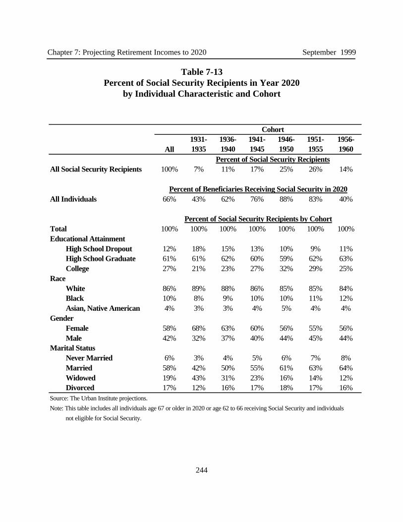
Chapter 7: Projecting Retirement Incomes to 2020 September 1999
244
Cohort
All1931-1935
1936-1940
1941-1945
1946-1950
1951-1955
1956-1960
Percent of Social Security RecipientsAll Social Security Recipients 100% 7% 11% 17% 25% 26% 14%
Percent of Beneficiaries Receiving Social Security in 2020All Individuals 66% 43% 62% 76% 88% 83% 40%
Percent of Social Security Recipients by CohortTotal 100% 100% 100% 100% 100% 100% 100%Educational Attainment
High School Dropout 12% 18% 15% 13% 10% 9% 11%High School Graduate 61% 61% 62% 60% 59% 62% 63%College 27% 21% 23% 27% 32% 29% 25%
RaceWhite 86% 89% 88% 86% 85% 85% 84%Black 10% 8% 9% 10% 10% 11% 12%Asian, Native American 4% 3% 3% 4% 5% 4% 4%
GenderFemale 58% 68% 63% 60% 56% 55% 56%Male 42% 32% 37% 40% 44% 45% 44%
Marital StatusNever Married 6% 3% 4% 5% 6% 7% 8%Married 58% 42% 50% 55% 61% 63% 64%Widowed 19% 43% 31% 23% 16% 14% 12%Divorced 17% 12% 16% 17% 18% 17% 16%
Source: The Urban Institute projections.
Note: This table includes all individuals age 67 or older in 2020 or age 62 to 66 receiving Social Security and individuals
not eligible for Social Security.
Table 7-13Percent of Social Security Recipients in Year 2020
by Individual Characteristic and Cohort

Chapter 7: Projecting Retirement Incomes to 2020 September 1999
245
and earnings are calculated year-by-year, but pensions and wealth are only projected to age 62 orage 67. Therefore our post retirement income is restricted to starting at age 62 or age 67. Individuals born in 1959 and 1960 are ages 61 and 60 respectively and, despite any SocialSecurity disability status, are not considered Social Security recipients in 2020. For those bornbetween 1954 and 1958 (age 63 to 66 in 2020), our 2020 population only includes those whoaccept Social Security at age 62. For example, only 43 percent of Social Security beneficiariesborn between 1931 and 1935 are projected to survive to 2020, and only 40 percent of those bornbetween 1956 and 1960 are projected to receive Social Security in 2020.
For the oldest Social Security recipients in our projection sample (those born between1931 and 1935), about 68 percent are female and about 43 percent are widowed. Theseproportions are both substantially higher than for the youngest Social Security recipients (thoseborn between 1956 and 1960). Of the youngest recipients, only 56 percent are female and 12percent are widowed. Except for the differential effect of mortality, the proportions of SocialSecurity beneficiaries by educational attainment, race, gender and marital status for each cohort in2020 are the same as at first benefit receipt (Table 7-6), but the differential effects of mortalitymatter for the earlier cohorts. Women, whites, and college educated all have higher lifeexpectancy. Therefore, for those born between 1931 and 1935, these groups are projected to be ahigher proportion of the cohort in 2020 than their respective shares at first Social Security benefitreceipt.
2. Sources of Income of Retirees in 2020
Average per capita income in 2020 of Social Security beneficiaries born between 1931 and1960 is projected to be 0.76 times the average wage (see Table 7-14). On average, SocialSecurity and returns from financial assets each account for about 40 percent of this income, butthis varies dramatically by income and demographic group. Social Security accounts for morethan half of the income of high school dropouts (0.22 versus 0.41 times the average wage), butonly a third of the income of college graduates (0.33 versus 1.05 times the average wage). Incontrast, income from financial assets accounts for only a quarter of the income of high schooldropouts and almost half (45 percent) of the income of college graduates. White Social Securityrecipients in 2020 have about 50 percent higher per capita income than black recipients (0.79versus 0.52).
Generally, average per capita income of Social Security beneficiaries in 2020 decreases asage increases. This reflects the combined effect of some sources of incomes not keeping up withaverage wage growth and cohort effects in the original accumulation of wealth. Two notableexceptions, however, are the youngest and the oldest cohorts. The youngest cohort of SocialSecurity beneficiaries are really a bimodal group. They include both relatively poor individuals,

Chapter 7: Projecting Retirement Incomes to 2020 September 1999
246
Per Capita Income/Average Wage by Income Source
Financial Asset Income1
Percent of Individuals Total
Social Security
Financial Income
DB Pension Income Earnings
Imputed Rental Income
DC Pension IRA Saving
Total 100% 0.76 0.29 0.28 0.08 0.04 0.06 0.11 0.03 0.14
Educational Attainment
High School Dropout 12% 0.41 0.22 0.10 0.03 0.02 0.04 0.03 0.01 0.07
High School Graduate 61% 0.69 0.29 0.24 0.07 0.04 0.05 0.10 0.03 0.12
College 27% 1.05 0.33 0.47 0.12 0.06 0.07 0.19 0.05 0.23
Race
White 86% 0.79 0.30 0.31 0.08 0.04 0.06 0.12 0.03 0.15
Black 10% 0.52 0.26 0.12 0.07 0.04 0.04 0.06 0.01 0.05
Asian, Native American 4% 0.71 0.26 0.27 0.07 0.04 0.06 0.10 0.03 0.14
Gender
Female 58% 0.72 0.29 0.26 0.08 0.03 0.06 0.10 0.03 0.13
Male 42% 0.80 0.29 0.32 0.08 0.05 0.06 0.13 0.03 0.16
Marital Status by Gender
Never Married 6% 0.70 0.25 0.28 0.08 0.03 0.06 0.11 0.03 0.14
Married 58% 0.76 0.29 0.30 0.08 0.05 0.05 0.11 0.03 0.15
Widowed 19% 0.78 0.31 0.27 0.10 0.02 0.08 0.11 0.03 0.13
Divorced 17% 0.73 0.30 0.26 0.08 0.04 0.06 0.12 0.03 0.11 Age
85 and Older 7% 0.77 0.29 0.30 0.10 0.00 0.07 0.05 0.01 0.25 80 to 84 11% 0.72 0.29 0.28 0.09 0.00 0.06 0.08 0.02 0.18 75 to 79 17% 0.72 0.29 0.29 0.08 0.00 0.06 0.11 0.03 0.16 70 to 74 25% 0.76 0.30 0.29 0.09 0.02 0.06 0.13 0.03 0.13 65 to 69 26% 0.78 0.30 0.28 0.08 0.08 0.06 0.13 0.04 0.11 62 to 64 14% 0.76 0.27 0.27 0.06 0.11 0.05 0.13 0.04 0.10
AIME Quintile at Age 62
1 20% 0.57 0.20 0.20 0.09 0.02 0.05 0.06 0.02 0.12
2 20% 0.58 0.25 0.19 0.05 0.03 0.05 0.06 0.03 0.11 3 20% 0.65 0.29 0.21 0.06 0.04 0.05 0.08 0.03 0.11 4 20% 0.81 0.34 0.29 0.08 0.05 0.06 0.13 0.04 0.13 5 20% 1.17 0.38 0.53 0.13 0.06 0.08 0.24 0.05 0.24
Per Capita Income Quintile1 20% 0.24 0.17 0.03 0.01 0.00 0.03 0.00 0.00 0.03 2 20% 0.44 0.28 0.07 0.03 0.01 0.04 0.02 0.01 0.05 3 20% 0.60 0.31 0.14 0.07 0.03 0.05 0.04 0.02 0.07 4 20% 0.85 0.34 0.28 0.12 0.05 0.07 0.10 0.04 0.13 5 20% 1.65 0.36 0.90 0.18 0.12 0.09 0.40 0.08 0.42
Source: The Urban Institute projections.1/ This allocation of financial asset income assumes proportionate consumption of initial assets by type of asset over time.
Table 7-14Average Per Capita Income as a Percent of the Average Wage in 2020
by Individual Characteristic and Income Source

Chapter 7: Projecting Retirement Incomes to 2020 September 1999
247
for whom Social Security provides a high replacement rate on earnings, and wealthier individualswho have chosen to retire early. Members of the oldest cohort in 2020 are systematicallyindividuals with long life expectancy. Longer life expectancy is generally correlated with higherincome, so not surprisingly, we find that the oldest old have on average higher per capita incomethan the younger old. Selective mortality affects income in all age groups, but is most notable inthe oldest group.
Despite the fact that later cohorts have higher financial assets than earlier cohorts at firstSocial Security benefit, the proportion of income that comes from financial assets is increasingwith increased age. For example, the youngest Social Security beneficiaries in 2020 receive about35 percent of their per capita income from financial assets (0.27/0.76). This proportion increasesfor the older ages, and the oldest beneficiaries in 2020 receive about 40 percent of their incomefrom financial assets (0.30/0.77). Two main factors contribute to this anomaly. First, those whosurvive to old age are more likely to be wealthy, which increases the average wealth of survivors,and second, our model of the rate of dissaving from wealth predicts that families do not reducetheir financial assets as fast as a full annuity model would predict. This means that potentialannuity income from non-annuitized wealth increases as people age. Both factors contribute tothe build up in the share of income that comes from financial assets by age.
Projected average per capita income of Social Security beneficiaries in the highest fifth ofthe income distribution in 2020 is more than six and a half times higher than for those in thelowest fifth of the income distribution. The sources of income vary dramatically among incomequintiles. Those in the bottom fifth of the distribution rely almost solely on Social Security, andthose in the top fifth of the income distribution have high income from a variety of sources. Thetop income group receives on average about a quarter of its income from Social Security and overhalf from financial assets (including DC pensions). Interestingly, for the top income recipients,earned income is still a significant share (seven percent) of total income, though these earnings arealmost entirely among the youngest beneficiaries.
The composition of financial assets changes by age group. Our model for the rate ofdissaving from financial assets does not distinguish dissaving by asset source. If, however,individuals and families dissave from each asset source at the same rate over time, the share offinancial assets from IRAs and DC balances increases for younger beneficiaries compared witholder beneficiaries along with a decrease in other financial wealth (wealth outside of retirementaccounts).
3. Changes in Poverty Rates of Retirees
Besides per capita income, an additional measure of well-being is family income relative tothe family poverty threshold. The poverty thresholds attempt to account for the economies ofshared resources including accommodations that married couples enjoy and the lower expenses

Chapter 7: Projecting Retirement Incomes to 2020 September 1999
248
that those over age 65 (and presumably not working) enjoy. In 1997, the poverty threshold for amarried couple under age 65 was $10,805. For a married couple age 65 and older, the povertythreshold was $9,712. For a single individual under age 65, the poverty threshold was $8,350,and for a single individual age 65 and older, the poverty threshold was $7,698. These povertythresholds are updated each year for increases in the CPI-U. Imputed rental income is notincluded in the Census measure of poverty, so we omit it in the income measure for thesecalculations. Otherwise, our income measure in the next two tables is the same as those usedearlier in the chapter.
The effect of the higher threshold for families and individuals under age 65 is that itsystematically reduces the income to poverty threshold of the youngest retirees, making the under65 population look worse off relative to the older population. To make the poverty rates for theunder 65 Social Security beneficiaries comparable to the 65 and over beneficiaries, we havecalculated poverty thresholds for the younger group using the older group thresholds.
In 2020, the average income of Social Security beneficiaries is projected to be about 3.8times the poverty threshold (see Table 7-15). Family income relative to poverty is higher for latercohorts (younger retirees) than for earlier cohorts (older retirees). We project that the income ofthe oldest beneficiaries, those born between 1931 and 1935, will be about 3.6 times poverty, andthe income of the youngest beneficiaries, those born between 1956 and 1960 using the over age65 thresholds, will be about 4 times poverty. This difference, in part, reflects the decline inincomes after retirement which older retirees (but not younger ones) have experienced. Note that,unlike per capita income, the income to poverty ratio for those born between 1931 and 1935 (age85 and older) exceeds the income to poverty ratio of those born between 1936 and 1940. This isbecause many more individuals are widowed in this higher age group, which means that theirincomes are measured relative to the single person poverty threshold. Before accounting forchanges in income, becoming widowed amounts to a doubling of income on a per capita basis, butonly a 26 percent increase in income on a poverty threshold basis.
As with per capita income, college educated beneficiaries have substantially higher incomerelative to poverty than beneficiaries with lower educational attainment in all age groups. Whitebeneficiaries have higher income relative to poverty than nonwhites in all age groups. Males havehigher income relative to poverty than females in all age groups, but the difference between malesand females is less among younger retirees, possibly reflecting the smaller number of youngerretired females who are widowed.
For many subgroups of the population, the ratio of income to poverty in 2020 is higher foryounger beneficiaries. For divorced and never married individuals in 2020, however, this is nottrue. For Social Security beneficiaries who never married, the average ratio of income to

Chapter 7: Projecting Retirement Incomes to 2020 September 1999
249
Cohort
All1931-1935
1936-1940
1941-1945
1946-1950
1951-1955
1956-1960
1956-
19601
Average Total Family Income as a Percent of Poverty
Total 3.80 3.55 3.48 3.62 3.86 4.06 3.77 4.04
Educational Attainment
High School Dropout 1.96 2.13 2.02 1.94 1.92 1.95 1.84 1.97
High School Graduate 3.43 3.37 3.24 3.22 3.47 3.62 3.44 3.67
College 5.38 5.30 5.12 5.33 5.19 5.66 5.50 5.89
Race
White 3.96 3.70 3.63 3.77 4.03 4.24 3.96 4.24
Black 2.52 2.34 2.08 2.33 2.60 2.78 2.46 2.63
Asian, Native American 3.57 2.56 3.12 3.44 3.59 3.86 3.84 4.07
Gender
Female 3.46 3.14 3.05 3.24 3.52 3.81 3.54 3.75
Male 4.27 4.43 4.20 4.19 4.30 4.37 4.07 4.40
Marital Status
Never Married 2.59 3.54 2.62 2.31 2.62 2.89 2.06 2.23
Married 4.55 4.59 4.39 4.42 4.54 4.72 4.46 4.75
Widowed 2.83 2.73 2.60 2.56 3.00 3.19 2.93 3.18
Divorced 2.71 2.95 2.56 2.77 2.75 2.78 2.47 2.68
AIME Quintile at Age 62
1 2.80 3.07 3.02 2.98 2.82 2.79 2.27 2.40
2 2.82 2.66 2.67 2.57 2.92 2.94 2.88 3.073 3.18 3.06 2.74 3.14 3.25 3.40 3.08 3.284 4.06 3.53 3.61 3.64 4.17 4.42 4.27 4.595 6.13 5.43 5.38 5.76 6.16 6.73 6.37 6.85
Per Capita Income Quintile1 1.14 1.14 1.14 1.16 1.18 1.15 1.00 1.072 2.15 2.05 2.03 2.03 2.22 2.27 2.05 2.173 3.05 2.76 2.75 2.88 3.17 3.29 2.99 3.184 4.30 3.83 3.80 4.00 4.38 4.75 4.33 4.615 8.36 8.01 7.70 8.03 8.37 8.83 8.52 9.16
Source: The Urban Institute projections.Note: Total family income excludes imputed rental income.This table includes all individuals age 67 or older in 2020 or age 62 to 66 receiving or not eligible for Social Security.1/ Poverty rate calculated with the age 65 and over poverty thresholds for all families.
Table 7-15Average Family Total Income as a Percent of Poverty in 2020
by Individual Characteristic and Cohort
Chapter 7: Projecting Retirement Incomes to 2020 September 1999
250
poverty is 3.5 for the oldest retirees, but is only 2.1 for the youngest retirees. For divorcedbeneficiaries, the average ratio of income to poverty is 3.0 for older retirees and 2.5 for youngerretirees. Married couples have higher ratios of income to poverty in all cohorts compared withsingle individuals. Their ratio of income to poverty is lower for younger than for older retirees,but only by a small amount.
We project that about 8.5 percent of Social Security beneficiaries in our sample will be inpoverty in the year 2020, but the proportion varies considerably by educational attainment, race,gender, marital status, and age (see Table 7-16). A little over 3 percent of college graduates willbe in poverty in 2020, compared with over 25 percent of high school dropouts. The impact of alack of education on poverty is expected to increase over time. For example, we project that 19percent of the oldest high school dropouts will be in poverty in 2020, while about 27 percent ofthe youngest dropouts will be in poverty.
Blacks are more likely to be in poverty in 2020 than whites. In 2020, we project thatabout 20 percent of black Social Security beneficiaries will be in poverty, while only a little under7 percent of white beneficiaries will be. The poverty impact of being both black and under-educated is projected to increase over time. For example, among black, high school dropouts, weproject about 27 percent of those born between 1931 and 1935 will be in poverty, compared withover 44 percent of those born between 1956 and 1960 (using the over 65 thesholds).
We project much higher poverty rates for unmarried individuals than for married couples. About 2.8 percent of married couples will be in poverty in the year 2020, while almost 30 percentof never married retirees, about 13 percent of widows, and 17 percent of divorced retirees will bein poverty.
The analysis of Social Security beneficiaries in 2020 by age is complicated by the fact thatour universe includes only beneficiaries (and individuals not eligible for benefits) and only thosewho survive to 2020. As described in Section V.1 of this chapter, this group faces selection intwo dimensions. First, the youngest beneficiaries are all early retirees, and second, the oldestbeneficiaries all have long life expectancy. To facilitate cross age comparisons, we compare ourprojected income and poverty rates of the 2020 Social Security beneficiaries with Social Securitybeneficiaries in the early 1990s.
We generated income and poverty statistics for the early 1990s by combining the 1990 to1993 SIPP panels. Annual family income is the sum of family income for the first 12 months ofthe panel, and family poverty threshold is the sum of the monthly poverty thresholds divided by12.6 To be consistent with the MINT population, we included only current Social Securityrecipients among those ages 62 and 66 and all individuals age 67 or older. The family income onthe SIPP is the sum of Social Security and other transfer income, pension income, earned

Chapter 7: Projecting Retirement Incomes to 2020 September 1999
251
Cohort
All1931-1935
1936-1940
1941-1945
1946-1950
1951-1955
1956-1960
1956-
19601
Percent of Individuals in Poverty in 2020
Total 8.5% 8.3% 8.6% 8.1% 7.9% 8.3% 10.3% 9.2%
Educational Attainment
High School Dropout 25.1% 19.1% 20.9% 22.0% 26.5% 29.7% 29.5% 27.2%
High School Graduate 7.8% 6.7% 7.6% 7.1% 7.5% 7.5% 10.1% 8.7%
College 3.1% 4.0% 3.4% 3.4% 3.1% 3.0% 2.2% 2.2%
Race
White 6.8% 6.7% 7.3% 6.8% 6.3% 6.7% 7.8% 6.8%
Black 19.6% 19.0% 19.6% 17.4% 19.2% 17.7% 26.1% 24.5%
Asian, Native American 15.0% 29.4% 15.8% 13.5% 13.1% 14.8% 14.6% 13.4%
Race by Education
Non-Black
High School Dropout 22.7% 17.9% 18.5% 20.4% 24.4% 27.1% 25.4% 23.2%
High School Graduate 6.6% 5.9% 6.8% 6.2% 6.5% 6.5% 7.8% 6.4%
College 2.7% 3.5% 3.4% 3.0% 2.5% 2.7% 2.1% 2.0%
Black
High School Dropout 36.0% 26.7% 32.1% 29.4% 36.6% 40.0% 47.2% 44.4%
High School Graduate 17.3% 17.5% 16.3% 14.5% 16.4% 14.7% 25.9% 24.2%
College 8.5% 10.4% 3.8% 9.5% 12.6% 7.8% 3.4% 3.4%
Gender
Female 10.7% 10.2% 11.8% 10.8% 10.4% 10.1% 12.0% 10.9%
Male 5.3% 4.4% 3.3% 4.0% 4.8% 6.0% 8.2% 6.9%
Marital Status
Never Married 29.4% 26.1% 27.6% 29.2% 28.9% 27.6% 35.0% 34.8%
Married 2.8% 2.8% 2.1% 2.2% 2.3% 2.9% 4.2% 3.6%
Widowed 12.6% 10.6% 13.6% 12.2% 12.9% 11.6% 16.3% 13.2%
Divorced 16.5% 14.9% 14.6% 15.6% 16.0% 17.7% 18.5% 16.2%Source: The Urban Institute projections.Notes: Total family income excludes imputed rental income.1/ Poverty rate calculated with the age 65 and over poverty thresholds for all families.
Table 7-16Percent of Individuals in Poverty in 2020 by Individual Characteristic and Cohort
Chapter 7: Projecting Retirement Incomes to 2020 September 1999
252
income, and income from assets. The SIPP measure of income from assets is the sum of interest,dividends, rental income, and royalties. The MINT measure of income from assets is based on theannuity the individual or couple could purchase with 80 percent of their financial assets. Thesetwo measures could be very different. Our measure includes some consumption of asset principal-- Census’s measure does not. Our measure does not vary with varying annual rates of return onassets -- Census’s measure does. Our measure includes some income from nonincome generatingassets, such as cars -- Census’s measure does not. To facilitate comparing incomes, we calculatedfamily income for the 1990s Social Security beneficiaries using the MINT measure of incomefrom assets.
As we have seen earlier in this chapter, educational attainment of Social Securityrecipients in 2020 is higher than in the early 1990s. Twelve percent of beneficiaries had a collegeeducation in the early 1990s, compared with 27 percent of beneficiaries in 2020 (see Table 7-17). The proportion of nonwhite Social Security beneficiaries is increasing. Ninety percent ofbeneficiaries in the early 1990s were white, while only 86 percent of beneficiaries in 2020 will be. The proportion of divorced Social Security beneficiaries is increasing and the proportion ofwidowed beneficiaries is decreasing. Six percent of beneficiaries in the early 1990s weredivorced, while 17 percent of beneficiaries in 2020 will be, and 32 percent of beneficiaries in theearly 1990s were widowed, while only 19 percent of beneficiaries in 2020 will be. This is thecumulative effect of increased life expectancy, which reduces the number of widows, and theincreasing number of beneficiaries entering retirement divorced. The share of young SocialSecurity beneficiaries is increasing. Eleven percent of the beneficiaries in the early 1990s wereages 62 to 64, while 14 percent of beneficiaries in 2020 will be. Despite increasing longevity, thesheer size of the younger cohorts in 2020 overwhelms the longevity effect.
Comparing the Census income measure to the MINT income measure in the 1990s showsthat the MINT measure is higher (column 3 and 4 on Table 7-17). Average family income usingthe Census measure is 3.1 times the poverty threshold. The MINT income measure increasesincome by about 10 percent to 3.4 times the poverty threshold. The MINT definition raisesmeasured income in all groups. Income is higher in the MINT measure because it includes somereturn of principal and income from assets (cars for example) that are not counted in the Censusmeasure, which counts only cash income.
The projected ratio of average income to poverty for Social Security beneficiaries is higherin 2020 than in the early 1990s. Comparing the MINT measure of income for the two groups,average income to poverty is 10 percent higher in 2020 than in the early 1990s (3.80 versus 3.44). Interestingly, though, average income to poverty is lower for all education groups in 2020 than inthe early 1990s and is especially low for high school dropouts. Average income to poverty isabout 20 percent lower for high school dropouts in 2020 compared to the early 1990s, and it isabout 7 percent lower for high school and college graduates. The increasing level of education ofthe population causes average incomes to increase even though the income of

Chapter 7: Projecting Retirement Incomes to 2020 September 1999
253
Census Measure UI Measure
Census Measure UI Measure
Early 1990s 2020 Early 1990s
Early 1990s 2020 Early 1990s
Early 1990s 2020
Percent of Retirees
Average Family Income / Poverty Threshold Percent of Retirees Below Poverty
Total 100% 100% 3.12 3.44 3.80 8.8% 8.0% 8.5%
Educational Attainment
High School Dropout 41% 12% 2.23 2.44 1.96 15.5% 14.5% 25.1%
High School Graduate 47% 61% 3.38 3.72 3.43 4.4% 3.9% 7.8%
College 12% 27% 5.22 5.77 5.38 2.2% 2.1% 3.1%
Race
White 90% 86% 3.23 3.57 3.96 7.1% 6.3% 6.8%
Black 8% 10% 2.00 2.08 2.52 25.9% 25.3% 19.6%
Asian, Native American 2% 4% 2.94 3.18 3.57 11.5% 12.8% 15.0%
Gender
Female 59% 58% 2.89 3.14 3.46 11.5% 10.6% 10.7%
Male 41% 42% 3.45 3.86 4.27 5.0% 4.4% 5.3%
Marital Status
Never Married 5% 6% 2.63 2.76 2.59 17.4% 16.2% 29.4%
Married 57% 58% 3.64 4.07 4.55 2.7% 2.4% 2.8%
Widowed 32% 19% 2.43 2.60 2.83 15.5% 14.4% 12.6%
Divorced 6% 17% 2.27 2.42 2.71 22.3% 21.2% 16.5%
Age
62 to 64 11% 14% 3.17 3.41 3.77 7.9% 7.9% 10.3%
62 to 641 11% 14% 3.50 3.77 4.04 6.8% 6.7% 9.2%
65 to 69 28% 26% 3.44 3.76 4.06 6.5% 5.9% 8.3%
70 to 74 24% 25% 3.18 3.50 3.86 7.9% 7.2% 7.9%
75 to 79 18% 17% 3.01 3.33 3.62 9.6% 9.0% 8.1%
80 and Older2 19% 18% 2.63 2.96 3.51 13.0% 11.8% 8.5%Source: The Urban Institute projections.Note: Total family income excludes imputed rental income.This table includes all individuals age 67 or older in 2020 or age 62 to 66 receiving or not eligible for Social Security.The early 1990s is the first 12 months of the 1990, 1991, 1992, and 1993 SIPP panels combined.The alternate income measure replaces property income with financial asset annuity income.1/ Poverty rate calculated with the age 65 and over poverty thresholds for all families.2/ The oldest retirees in the MINT database in 2020 are 89 years old. The 1990 poverty numbers include all retirees over age 89.
Table 7-17Percent of Retirees, Average Family Income as a Percent of Poverty,
and Percent of Retirees Below Povertyby Individual Characteristic in the Early 1990s and 2020

Chapter 7: Projecting Retirement Incomes to 2020 September 1999
254
each education group is falling. In contrast, average income to poverty is higher for all racecategories in 2020 than in the early 1990s, with blacks doing significantly better in the 2020s thanin the early 1990s. The ratio of average income to poverty increased by over 20 percent forblacks and by about 11 percent for whites. Divorced Social Security beneficiaries have about 12percent higher income to poverty ratios in 2020 than those in the early 1990s, but never marriedbeneficiaries have about six percent lower income to poverty ratios than those in the early 1990s. Average income to poverty is also higher for all age groups in 2020 compared to the early 1990s. The youngest beneficiaries have about 10 percent higher ratios of income to poverty in 2020 thanthe youngest beneficiaries in the early 1990s. The oldest beneficiaries have about a 18 percenthigher ratio of income to poverty in 2020 than the oldest beneficiaries in the early 1990s, althoughthis statistic is not completely comparable, because the 1990 population includes individuals age90 and older (about three percent of Social Security beneficiaries) and the 2020 population doesnot.
While family income relative to the poverty threshold is increasing from the early 1990scompared to 2020, the proportion of the population with income below poverty is also increasing. Using the MINT definition of asset income, eight percent of Social Security beneficiaries were inpoverty in the early 1990s, and we project that 8.5 percent of beneficiaries will be in poverty in2020. The poverty rate of the under-educated is increasing. For example, 14.5 percent of highschool dropout beneficiaries were in poverty in the early 1990s, but we project that a much higher25.1 percent of the 2020 dropouts will be. There are fewer dropouts in 2020 (12 percent in 2020compared to 41 percent in 1990), but those without higher education in 2020 are much morelikely to end up in poverty than less-educated retirees in the early 1990s.
While the poverty rate for blacks continues to be higher than the poverty rate for whites,black Social Security beneficiaries in 2020 are doing better than those in the early 1990s. A littleover 25 percent of blacks were in poverty in the early 1990s, and 20 percent will be in poverty in2020. Poverty rates for both men and women are higher in 2020 than in the early 1990s, butmore so for men than for women. On the other hand, women are a larger share of the agedpopulation and have about twice the poverty rate as men in both 1990 and 2020.
Social Security beneficiaries who never married are much more likely to be in poverty in2020 than in the early 1990s. Sixteen percent of the never married beneficiaries were in povertyin the early 1990s, and over 29 percent are projected to be in poverty in 2020. Divorcedbeneficiaries, on the other hand, are less likely to be in poverty in 2020 compared to the early1990s. Twenty-one percent of the early 1990 divorced beneficiaries were in poverty, and only16.5 percent of the 2020 divorced beneficiaries will be. Married beneficiaries continue to have alow probability of being in poverty, but the poverty rate among them is rising slightly.

Chapter 7: Projecting Retirement Incomes to 2020 September 1999
255
Younger Social Security beneficiaries are more likely to be in poverty in 2020 than theywere in the early 1990s. Using the over age 65 poverty thresholds, over 9 percent of the 62- to64-year-old beneficiaries will be in poverty in 2020, compared with just 6.7 percent in the early1990s. Poverty rates are higher for all age groups in 2020 compared to the early 1990s up untilage 75 and older, at which point the poverty rates of the oldest retirees is lower in 2020 than in1990. The combined effect of MINT missing the oldest old and increased longevity means thatthe oldest beneficiaries in 2020 have not confronted the dramatic decline in financial assets thatoccurs in the last year of life. Both of these factors reduce the poverty rates of the oldestbeneficiaries in 2020 compared to the early 1990s. Also, we assumed that all DB pensions arejoint and survivor pensions. Although pension plans are required to allow spouses to elect a jointand survivor annuity, some people may still choose a single survivor annuity, especially if thespouse has other sources of income. To the extent that some DB beneficiaries do not choose jointand survivor pensions, our estimates overstate the incomes of the oldest beneficiaries in oursample and understate the incomes of the younger beneficiaries. If no married DB beneficiarieschoose joint and survivor pensions, the poverty rate from assuming no joint and survivor annuitiesof the oldest beneficiaries in 2020 would increase modestly from 8.5 percent to 9.1 percent, whichwould still be much lower than the poverty rate for the oldest beneficiaries in the early 1990s. The impact on poverty is even smaller for younger beneficiaries because mortality has not had asbig an impact on them and a lower proportion of younger beneficiaries have DB pensions.7
About 55 percent of the MINT population in 2020 who are not entitled to Social Securitybenefits are in poverty, but this percent varies by age. These are individuals who do not haveenough quarters of covered employment to be eligible for a retired worker benefit and who alsodo not qualify for a spouse or survivor benefit. About 78 percent of survivors between age 62and 64 in 2020 who are never eligible for Social Security benefits are in poverty compared toabout 46 percent of those age 80 and older. This difference reflects both the higher mortalityrates of poorer individuals and the higher share of beneficiaries entering retirement with noentitlement to Social Security. Higher divorce rates for later cohorts causes more former wives toenter retirement with no entitlement to their former spouse’s Social Security. While those noteligible for Social Security are a small proportion of the aged (about 4.5 percent) they are verylikely to be in poverty. While SSI, which we do not project, would provide some income to thesebeneficiaries, SSI income is not high enough to lift them out of poverty. They are still a veryvulnerable group. Appendix Table 7-A-4 shows the percent of the 2020 population with incomefrom each income source. Those without Social Security entitlement are more likely to be black,under educated, and never married.
VI. CONCLUSIONS
In this chapter, we have estimated changes in income and wealth as people age afterretirement, compared incomes of different cohorts and demographic groups at retirement, andprojected income of retirees of the 1931 to 1960 birth cohorts to the year 2020. We have

Chapter 7: Projecting Retirement Incomes to 2020 September 1999
256
examined trends in the distribution of income among successive cohorts of retirees and comparedthe population of Social Security recipients in 2020 with those in the early 1990s.
The rate of change of financial wealth for single and married retirees varies by age andother economic and demographic characteristics, including homeownership, race, presence of apension, presence of high earnings, widowhood status, and mortality. For most groups, financialwealth declines with age. The decline in financial wealth with age is relatively larger forhomeowners compared with renters, blacks compared with whites, families with pensionscompared with those without them, individuals outside of the highest earning group comparedwith high earners, and widows compared with divorced people and those never married.
The proportion of Social Security beneficiaries who are nonwhite and unmarried isincreasing over time. This change leads to an increase in the proportion of Social Securitybeneficiaries with lower incomes over time. At the same time, educational attainment and femalelabor force participation are increasing over time. This change leads to an increase in theproportion of Social Security beneficiaries with higher incomes over time. These demographicchanges along with increases in life expectancy and the sheer size of the Baby Boom cohorts willchange the fundamental composition of Social Security beneficiaries over time. These changesaffect both the accumulation of assets and the rate of consumption from these assets forsuccessive cohorts of Social Security beneficiaries out to the year 2020 and beyond.
For new retirees, Social Security and income from financial assets (other than DBpensions) are the two most important components of income, with Social Security being only aslightly higher share of total income. Social Security benefits are about 28 percent of the averagewage on average and they account for about 34 percent of total income at initial retirement. Social Security is a more important source of total income for blacks and lower educatedindividuals then for whites and those with a college education.
Financial assets are an important source of income for those Social Security beneficiarieswith financial assets, but financial assets are very unevenly distributed. College educatedbeneficiaries and whites have the bulk of these assets. Nonwhites and high school dropouts havecomparatively little savings at retirement. Earnings are an important source of income for manyof the elderly at initial Social Security receipt. Earnings are a relatively more important source ofincome for individuals with the highest incomes. Overall, Social Security benefits are the mostimportant income source for lower income groups and financial assets and earned income themost important source for people in the top income quintile.
Total income at first retirement will peak for Social Security beneficiaries born between1946 and 1950 and is projected to decline for post 1950 birth cohorts. Social Security andincome from financial assets (including income from DC plans) are increasing as a share of income

Chapter 7: Projecting Retirement Incomes to 2020 September 1999
257
for more recent birth cohorts, and DB pension income is decreasing as a share of income for morerecent cohorts.
Per capita income of Social Security recipients at initial receipt is quite unevenlydistributed, with individuals in the highest income quintile having about 7.1 times as much incomeas individuals in the lowest quintile. Over time, this differential is increasing. Incomes areincreasing in the highest quintile and decreasing in the lowest quintile.
Older Social Security beneficiaries in 2020 are more likely to be widowed women thanyounger Social Security beneficiaries. Older beneficiaries, because of the differential impact ofmortality, are also more likely to be white, higher educated, and higher income.
Comparisons of projected Social Security beneficiaries in 2020 with those in the early1990s show that the average income of future beneficiaries is projected to increase, but povertyrates will also increase. This occurs because incomes are becoming more unevenly distributed. Family well-being is highly correlated with marital status, educational attainment, and race. Married couples have more income than single individuals, higher educated individuals have moreincome than lower educated individuals, and whites have more income than nonwhites.
Educational attainment of Social Security beneficiaries in 2020 is higher than that of SocialSecurity beneficiaries in the early 1990s. Higher educated beneficiaries are more likely to bewealthy. Social Security beneficiaries in 2020 are more likely to be nonwhite, divorced, and ornever married compared to beneficiaries in the early 1990s. These groups are more likely to bepoor. These demographic changes are contributing to higher incomes for those better off andhigher poverty rates for those worse off. Those most at risk in 2020 are the less educated singlebeneficiaries. These groups are an increasing proportion of the youngest beneficiaries in 2020.Many of them will begin their retirement in poverty, and, if the past is a guide, the incidence ofpoverty in this cohort will increase as they age.

Chapter 7: Projecting Retirement Incomes to 2020 September 1999
258
APPENDIX A
TABLE 7-A-1Increases in Full Retirement Age and Delayed Retirement Credits, with Resulting Benefit,
As a Percent of Primary Insurance Amount [PIA], Payable at Selected Ages, for Persons Born in 1924 or Later--------------------------------------------------------------------------------------------------------------------- Credit for each Benefit, as a percent of PIA, beginning at age-- "Normal year of delayed ------------------------------------------------------ Year of birth Age 62 retirement retirement attained in-- age" after normal 62 65 66 67 70 retirement age ---------------------------------------------------------------------------------------------------------------------1924........... 1986........... 65......... 3 80 100 103 106 1151925-26........ 1987-88........ 65......... 3 1/2 80 100 103 1/2 107 117 1/2 1927-28........ 1989-90........ 65......... 4 80 100 104 108 1201929-30........ 1991-92........ 65......... 4 1/2 80 100 104 1/2 109 122 1/2 1931-32........ 1993-94........ 65......... 5 80 100 105 110 1251933-34........ 1995-96........ 65......... 5 1/2 80 100 105 1/2 111 127 1/2 1935-36........ 1997-98........ 65......... 6 80 100 106 112 1301937........... 1999........... 65......... 6 1/2 80 100 106 1/2 113 132 1/2 1938........... 2000........... 65, 2 mo... 6 1/2 79 1/6 98 8/9 105 5/12 111 11/12 131 5/12 1939........... 2001........... 65, 4 mo... 7 78 1/3 97 7/9 104 2/3 111 2/3 132 2/3 1940........... 2002........... 65, 6 mo... 7 77 1/2 96 2/3 103 1/2 110 1/2 131 1/2 1941........... 2003........... 65, 8 mo... 7 1/2 76 2/3 95 5/9 102 1/2 110 132 1/2 1942........... 2004........... 65, 10 mo.. 7 1/2 75 5/6 94 4/9 101 1/4 108 3/4 131 1/4 1943-54........ 2005-16........ 66......... 8 75 93 1/3 100 108 1321955........... 2017........... 66, 2 mo... 8 74 1/6 92 2/9 98 8/9 106 2/3 130 2/3 1956........... 2018........... 66, 4 mo... 8 73 1/3 91 1/9 97 7/9 105 1/3 129 1/3 1957........... 2019........... 66, 6 mo... 8 72 1/2 90 96 2/3 104 1281958........... 2020........... 66, 8 mo... 8 71 2/3 88 8/9 95 5/9 102 2/3 126 2/3 1959........... 2021........... 66, 10 mo.. 8 70 5/6 87 7/9 94 4/9 101 1/3 125 1/3 1960 or later.. 2022 or later.. 67......... 8 70 86 2/3 93 1/3 100 124--------------------------------------------------------------------------------------------------------------------Source: Table 1-8 from Committee on Ways and Means U.S. House of Representatives, Green Book (1996).

Chapter 7: Projecting Retirement Incomes to 2020 September 1999
Family Income SourceFinancial Asset Income
Percent of Individuals
Total Income
Social Security
Financial Income
DB Pension Income
Earned Income
Imputed Rental Income
DC Pension Income
IRA Income
Saving Income
Average Per Capita Income/Average Wage by Income SourceTotal 100% 0.82 0.28 0.25 0.09 0.15 0.06 0.11 0.03 0.12Educational Attainment
High School Dropout 13% 0.46 0.22 0.09 0.04 0.08 0.04 0.03 0.00 0.06High School Graduate 60% 0.76 0.28 0.21 0.08 0.14 0.05 0.09 0.02 0.10College 26% 1.16 0.31 0.44 0.14 0.20 0.07 0.18 0.05 0.20
RaceWhite 85% 0.86 0.28 0.27 0.10 0.15 0.06 0.11 0.03 0.13Black 11% 0.59 0.25 0.11 0.08 0.11 0.03 0.06 0.01 0.04Asian, Native American 4% 0.77 0.25 0.24 0.07 0.15 0.06 0.10 0.03 0.12
GenderFemale 54% 0.79 0.28 0.23 0.09 0.13 0.06 0.10 0.03 0.11Male 46% 0.86 0.27 0.27 0.10 0.17 0.06 0.11 0.03 0.13
Marital Status by GenderNever Married Female 3% 0.75 0.26 0.21 0.11 0.12 0.06 0.10 0.02 0.10Never Married Male 2% 0.80 0.28 0.29 0.08 0.08 0.06 0.12 0.03 0.15Married Women 32% 0.80 0.27 0.25 0.09 0.14 0.05 0.10 0.03 0.13Married Men 35% 0.84 0.25 0.26 0.09 0.19 0.05 0.10 0.03 0.13Widowed Female 9% 0.83 0.32 0.24 0.12 0.09 0.07 0.13 0.04 0.07Widowed Male 2% 1.03 0.36 0.34 0.16 0.10 0.08 0.18 0.04 0.12Divorced Female 10% 0.73 0.30 0.18 0.08 0.12 0.06 0.09 0.02 0.07Divorced Male 6% 0.94 0.35 0.30 0.13 0.10 0.07 0.15 0.03 0.12
Cohort1931-1935 11% 0.83 0.28 0.20 0.15 0.14 0.06 0.03 0.01 0.161936-1940 12% 0.82 0.28 0.21 0.12 0.15 0.06 0.06 0.02 0.141941-1945 15% 0.83 0.28 0.24 0.10 0.16 0.06 0.09 0.02 0.131956-1950 19% 0.85 0.28 0.27 0.09 0.15 0.06 0.12 0.03 0.121951-1955 21% 0.82 0.28 0.27 0.08 0.14 0.06 0.12 0.04 0.111956-1960 23% 0.79 0.27 0.28 0.07 0.13 0.05 0.15 0.04 0.09
AIME Quintile1 20% 0.58 0.18 0.17 0.10 0.08 0.05 0.05 0.02 0.102 20% 0.62 0.24 0.17 0.05 0.11 0.05 0.05 0.02 0.093 20% 0.72 0.28 0.19 0.07 0.13 0.05 0.07 0.02 0.094 20% 0.91 0.33 0.26 0.10 0.17 0.06 0.12 0.03 0.115 20% 1.29 0.36 0.48 0.15 0.23 0.08 0.23 0.05 0.21
Per Capita Income Quintile1 20% 0.25 0.17 0.03 0.01 0.01 0.03 0.00 0.00 0.032 20% 0.47 0.27 0.07 0.04 0.05 0.04 0.02 0.01 0.053 20% 0.67 0.30 0.14 0.08 0.10 0.05 0.04 0.02 0.074 20% 0.95 0.32 0.26 0.13 0.18 0.07 0.10 0.04 0.125 20% 1.78 0.34 0.76 0.20 0.39 0.09 0.36 0.07 0.33
Source: The Urban Institute projections.
Table 7-A-2Percent of Individuals and Average Per Capita Income as a Percent of the Average Wage
at the Individual's Initial Social Security Benefit Receiptby Income Source and Income Source

Chapter 7: Projecting Retirement Incomes to 2020 September 1999
Family Income SourceFinancial Asset Income
Percent of Individuals
Total Income
Social Security
Financial Income
DB Pension Income
Earned Income
Imputed Rental Income
DC Pension Income
IRA Income
Saving Income
Percent of Individuals Receiving Family Income by Income SourceTotal 100% 1.00 0.96 0.94 0.48 0.46 0.91 0.36 0.30 0.91Educational Attainment
High School Dropout 13% 0.99 0.91 0.89 0.33 0.33 0.84 0.17 0.10 0.87High School Graduate 60% 1.00 0.97 0.94 0.49 0.46 0.91 0.35 0.27 0.91College 26% 1.00 0.97 0.97 0.55 0.54 0.94 0.46 0.49 0.94
RaceWhite 85% 1.00 0.97 0.96 0.49 0.48 0.93 0.37 0.33 0.93Black 11% 0.99 0.94 0.85 0.46 0.36 0.78 0.25 0.09 0.81Asian, Native American 4% 1.00 0.94 0.89 0.42 0.45 0.86 0.31 0.25 0.85
GenderFemale 54% 1.00 0.96 0.94 0.48 0.41 0.90 0.34 0.30 0.90Male 46% 1.00 0.97 0.95 0.49 0.53 0.92 0.38 0.31 0.93
Marital Status by GenderNever Married Female 3% 0.98 0.85 0.87 0.38 0.28 0.66 0.26 0.19 0.83Never Married Male 2% 0.98 0.86 0.88 0.33 0.26 0.65 0.22 0.23 0.82Married Women 32% 1.00 0.96 0.97 0.51 0.47 0.96 0.39 0.35 0.95Married Men 35% 1.00 0.97 0.97 0.51 0.60 0.96 0.41 0.34 0.95Widowed Female 9% 1.00 0.98 0.88 0.52 0.32 0.87 0.25 0.26 0.83Widowed Male 2% 1.00 0.98 0.90 0.54 0.28 0.87 0.28 0.24 0.85Divorced Female 10% 1.00 0.97 0.88 0.34 0.32 0.80 0.25 0.18 0.83Divorced Male 6% 1.00 0.96 0.89 0.40 0.28 0.82 0.28 0.21 0.83
Cohort1931-1935 11% 1.00 0.95 0.94 0.52 0.45 0.94 0.23 0.42 0.911936-1940 12% 1.00 0.95 0.94 0.48 0.46 0.93 0.33 0.38 0.911941-1945 15% 1.00 0.95 0.95 0.48 0.47 0.92 0.36 0.34 0.921956-1950 19% 1.00 0.96 0.95 0.48 0.47 0.91 0.39 0.31 0.921951-1955 21% 1.00 0.97 0.94 0.48 0.47 0.90 0.38 0.27 0.911956-1960 23% 1.00 0.98 0.94 0.47 0.45 0.88 0.38 0.21 0.91
AIME Quintile1 20% 0.99 0.81 0.90 0.38 0.32 0.85 0.22 0.21 0.872 20% 1.00 1.00 0.92 0.39 0.38 0.87 0.26 0.23 0.893 20% 1.00 1.00 0.95 0.48 0.44 0.90 0.34 0.26 0.914 20% 1.00 1.00 0.97 0.55 0.53 0.94 0.42 0.33 0.935 20% 1.00 1.00 0.99 0.61 0.64 0.98 0.53 0.48 0.97
Per Capita Income Quintile1 20% 0.99 0.89 0.84 0.19 0.19 0.76 0.09 0.06 0.822 20% 1.00 0.98 0.94 0.43 0.35 0.90 0.22 0.17 0.903 20% 1.00 0.98 0.97 0.57 0.49 0.94 0.35 0.30 0.934 20% 1.00 0.98 0.98 0.62 0.60 0.96 0.48 0.43 0.955 20% 1.00 0.98 0.99 0.60 0.69 0.97 0.64 0.56 0.97
Source: The Urban Institute projections.
Table 7-A-3Percent of Individuals Receiving Family Income by Income Source
at the Individual's Initial Social Security Benefit Receipt

Chapter 7: Projecting Retirement Incomes to 2020 September 1999
Per Capita Income/Average Wage by Income Source
Financial Asset Income1
Percent of Individuals Total
Social Security
Financial Assets
DB Pension Earnings
Imputed Rent
DC Pension IRA Saving
Total 100% 1.00 0.97 0.95 0.53 0.15 0.91 0.37 0.32 0.92
Educational Attainment
High School Dropout 12% 0.99 0.92 0.89 0.35 0.09 0.84 0.18 0.09 0.88
High School Graduate 61% 1.00 0.98 0.94 0.53 0.15 0.91 0.36 0.28 0.91
College 27% 1.00 0.98 0.98 0.60 0.18 0.94 0.47 0.51 0.94
Race
White 86% 1.00 0.98 0.96 0.53 0.16 0.93 0.38 0.35 0.93
Black 10% 0.99 0.94 0.86 0.50 0.14 0.78 0.27 0.10 0.81
Asian, Native American 4% 0.99 0.94 0.91 0.46 0.16 0.87 0.33 0.27 0.86
Gender
Female 58% 1.00 0.97 0.94 0.52 0.12 0.91 0.35 0.31 0.90
Male 42% 1.00 0.97 0.96 0.54 0.20 0.92 0.40 0.33 0.93
Marital Status by Gender
Never Married 6% 0.98 0.84 0.89 0.36 0.10 0.67 0.25 0.22 0.84
Married 58% 1.00 0.98 0.98 0.58 0.20 0.97 0.43 0.36 0.96
Widowed 19% 1.00 0.98 0.92 0.54 0.07 0.91 0.29 0.32 0.88
Divorced 17% 1.00 0.96 0.89 0.38 0.10 0.82 0.28 0.21 0.84 Age
85 and Older 7% 1.00 0.97 0.95 0.59 0.00 0.94 0.25 0.46 0.92 80 to 84 11% 1.00 0.97 0.95 0.55 0.01 0.93 0.34 0.40 0.91 75 to 79 17% 1.00 0.97 0.95 0.54 0.01 0.92 0.37 0.35 0.92 70 to 74 25% 1.00 0.97 0.95 0.54 0.06 0.92 0.39 0.32 0.92 65 to 69 26% 1.00 0.97 0.94 0.51 0.27 0.91 0.39 0.27 0.91 62 to 64 14% 1.00 0.97 0.94 0.48 0.47 0.88 0.37 0.23 0.91
AIME Quintile at Age 62
1 20% 0.99 0.86 0.90 0.42 0.11 0.86 0.24 0.23 0.87
2 20% 1.00 1.00 0.92 0.43 0.13 0.88 0.26 0.25 0.89 3 20% 1.00 1.00 0.95 0.53 0.15 0.91 0.36 0.27 0.91 4 20% 1.00 1.00 0.97 0.60 0.17 0.94 0.44 0.35 0.94 5 20% 1.00 1.00 0.99 0.66 0.20 0.98 0.55 0.49 0.97
Per Capita Income Quintile1 20% 0.99 0.90 0.84 0.23 0.06 0.77 0.08 0.05 0.81 2 20% 1.00 0.99 0.94 0.47 0.11 0.91 0.22 0.17 0.90 3 20% 1.00 0.99 0.98 0.62 0.15 0.95 0.35 0.32 0.94 4 20% 1.00 0.99 0.99 0.69 0.19 0.97 0.51 0.45 0.96 5 20% 1.00 0.98 1.00 0.63 0.25 0.98 0.68 0.60 0.97
Source: The Urban Institute projections.1/ This allocation of financial asset income assumes equal consumption of initial assets by type of asset over time.
Percent of Individuals with Family Income by Income Source
Table 7-A-4Percent of Individuals with Family Income by Income Source in 2020
by Individual Characteristic and Income Source

Chapter 7: Projecting Retirement Incomes to 2020 September 1999
262
CHAPTER 7: REFERENCES
Lubitz, Jim, J. Beebe, and C. Baker, “Longevity and Medicare Expenditures,” New EnglandJournal of Medicine, April 13, 1995.
McNeil, Jack, and Enrique Lamas, 1988. “Year-Apart Estimates of Household Net Worth Fromthe Survey of Income and Program Participation,” Bureau of the Census, No. 8804.
Smith, Karen and Eric Toder, “Subtask 7.2 - Test Alternatives for Projecting Retirement Incomeand Assets From Early Retirement Age Until Death,” Letter Report, March 31, 1999.
CHAPTER 7: LIST OF TABLES
Table 7-1Date of Master Beneficiary Record Information by SIPP Panel 215
Table 7-2Average Annual Growth in Average Wage and CPI-U--1980 to 2019
216Table 7-3
OLS Regression Results by Marital Status for Dependent Variable LogFinancial Assets 218
Table 7-4OLS Regression Results for Married Couplesfor Dependent Variable Log Financial AssetsPercent Change in Financial Assets and Standard Error Per Year of Age 221
Table 7-5OLS Regression Results for Single Individualsfor Dependent Variable Log Financial AssetsPercent Change in Financial Assets and Standard Error Per Year of Age 224
Table 7-6Percent of Individuals at Initial Social Security Receipt by Individual Characteristic and Cohort 228
Table 7-7Sources of Changes in Projected Financial Assets by Individual Characteristic at InitialSocial Security Benefit Receipt and Cohort 230
Table 7-8Percent of Husbands and Average Family Income Divided by the Average Wage at the Husband's Initial Social Security Benefit Receipt byIndividual Characteristic and Income Source 233

Chapter 7: Projecting Retirement Incomes to 2020 September 1999
263
Table 7-9Percent of Total Family Income by Family Income Sourceat Husband's Initial Social Security Benefit Receipt for Married Couplesby Individual Characteristic and Income Source 234
Table 7-10Percent of Wives and Average Family Income Divided by the Average Wageat the Wife's Initial Social Security Benefit Receiptby Individual Characteristic and Income Source 237
Table 7-11Percent of Single Individuals and Average Family Income Divided by the Average Wage at Single Individual's Initial Social Security Benefit Receiptby Individual Characteristic and Income Source 239
Table 7-12Average Per Capita Income as a Percent of the Average Wage at Initial Social Security Benefit Receipt by Gender, Cohort, and Per Capita Income Quintile 242
Table 7-13Percent of Social Security Recipients in Year 2020by Individual Characteristic and Cohort 244
Table 7-14Average Per Capita Income as a Percent of the Average Wage in 2020by Individual Characteristic and Income Source 246
Table 7-15Average Family Total Income as a Percent of Poverty in 2020by Individual Characteristic and Cohort 249
Table 7-16Percent of Individuals in Poverty in 2020 by Individual Characteristic and Cohort 251
Table 7-17Percent of Retirees, Average Family Income as a Percent of Poverty,and Percent of Retirees Below Povertyby Individual Characteristic in the Early 1990s and 2020 253
TABLE 7-A-1Increases in Full Retirement Age and Delayed Retirement Credits, with Resulting Benefit, As a Percent of Primary Insurance Amount [PIA], Payable at Selected Ages, for PersonsBorn in 1924 or Later 258
Table 7-A-2Percent of Individuals and Average Per Capita Income as a Percent of the Average Wageat the Individual's Initial Social Security Benefit Receiptby Income Source and Income Source 259
Chapter 7: Projecting Retirement Incomes to 2020 September 1999
264
1. This model specification does not include wealth in the base period, as described in our letterreport 7.1 to SSA. McNeil and Lamas (1988) found that the annual variation in reported wealthbetween the two financial asset topical modules was not reliable. Therefore, we rejected using afixed-effects specification.
2. The SIPP wealth topical modules for the 1990s ask about 401(k) balances. Our sample,however, is limited to families with heads age 62 or older in 1984. 401(k) plans did not start beingpopular until the mid-1980s. By then, most of our sample would have retired, and would not havehad an opportunity to accumulate any savings in them.
3. The parameter estimates are in the logarithmic scale and are close approximations of percentchange for small values (less than five percent). The parameter estimate for the last year of life(-23.26=-20.7-2.56) in the nominal scale is 20.7 percent per year of age.
4. The parameter estimates are in the logarithmic scale and are close approximations of percentchange for small values (less than five percent). The parameter estimate for the last year of life(-29.25=-25.6-3.65) in the nominal scale is 25.3 percent per year of age.
5. Beginning with individuals born after 1937, the “normal retirement age” is scheduled to increasefrom age 65 by two months for every year until it reaches age 66 for the 1943 cohort. It remains at
Table 7-A-3Percent of Individuals Receiving Family Income by Income Sourceat the Individual's Initial Social Security Benefit Receipt 260
Table 7-A-4Percent of Individuals with Family Income by Income Source in 2020by Individual Characteristic and Income Source 261
CHAPTER 7: LIST OF FIGURES
Figure 7-1Amount and Composition of Wealth by AgeFinancial Asset Saver 213
Figure 7-2Amount and Composition of Wealth by AgePermanent Income Dissaver 213
Figure 7-3Percent of Workers With Earnings Below the Taxable Maximumfor Men and Women by Year 219
CHAPTER 7: ENDNOTES

Chapter 7: Projecting Retirement Incomes to 2020 September 1999
265
age 66 until it again increases for cohorts born after 1954 by two months for every year until itreaches age 67 for the 1960 cohort. Along with the increase in the age of normal retirement, theactuarial reduction will increase by 5/12 of one percent for every month in excess of 36 months. Thisgradually increases the maximum reduction from 20 percent for the 1938 cohort to 30 percent for the1960 cohort.
The delayed retirement credit is also increasing over time, but at later ages. See Appendix 7-A-1 for more information in the impact of legislated changes in Social Security by cohort.
6. The SIPP reports annual poverty thresholds for each month. A family is in poverty in a particularmonth if its monthly family income is less than the annual poverty threshold divided by 12. A familyis in poverty in a year if its annual income is below their average annual poverty threshold.
7. If no DB beneficiaries chose joint and survivor pensions, projected poverty rates would be10.1 percent for 62- to 64-year-olds (using the over 65 thresholds), 8.1 percent for the 65- to 69-year-olds, 8.3 percent for the 70-to-74-year-olds, 9.2 percent for the 75- to 79-year-olds, and 9.1percent for those age 80 and older.

266
CHAPTER 8
STYLIZED EARNINGS FOR BIRTH COHORTS 1931-60
I. INTRODUCTION
This chapter presents stylized earnings profiles for workers in birth cohorts 1931-60. Itdisplays the patterns of Social Security qualifying earnings between three periods of a worker’scareer -- ages 31-40, 41-50, and 51-60. It divides workers into groups based on the level andshape of their career earnings patterns and then displays the earnings patterns for the average ortypical workers in each group. Separate earnings patterns are shown for male and femaleworkers.
The next section of the chapter discusses the methodology used. The following sectiondisplays some preliminary earnings patterns for workers in the 1931-40 birth cohort who havecompleted their working careers. This was the basis for much of the initial exploration of thecharacteristics of the earnings patterns. The last section creates patterns for all the 1931-60 birthcohorts, based on the projections of earnings reported in Chapter 2.
II. BASIC METHODOLOGY
Individuals’ earnings are expressed as relatives by dividing each year’s earnings by theeconomy-wide average wage of that year. Because the reported earnings are truncated by thetaxable wage ceiling of each year, we adjusted earnings of those at the ceiling to put them on abasis that is consistent with the current relationship of the taxable ceiling to the average wage.1 The wage data are then lined up by age, and we developed a classification system based on thepattern of individuals’ earnings from age 32 through age 61.2 We excluded earnings for agesbelow 32 because nearly all workers had rising earnings over this period and some individualshave very low earnings because they are still in school. We computed the average of the earningsrelatives in each of the three 10-year sub-periods extending from age 32 through age 61, labeledas A, B, and C.
Workers are classified in terms of three characteristics: (1) their “lifetime wage” computedas the average of their wage relatives over the 30-year period (low, middle, and high), (2) thetrend change in the relative wage between sub-periods A and C (falling, level, rising), and (3) aprofile based on whether the average wage during period B differs from the average of A and C(sag, level, humped):

Chapter 8: Stylized Earnings for Birth Cohorts 1931-60 September 1999
267
Trend
t = (C-A) / (C+A)Declining t < -1/9Level -1/9 < t > 1/9Increasing t > 1/9
Profile
p = (B -(A+C)/2 ) / (B + (A+C)/2)Sag p < -1/9linear -1/9 < p > 1/9humped p > 1/9
The three categories of the 30-year average wage were computed as equal thirds of thedistribution of “lifetime” wages for all the birth cohorts between 1931 and 1960. The middle classinterval was from 0.37 to 1.04 of the average wage.3 The cutoffs for the trend and profilecharacteristics were chosen to be symmetric and yield roughly a third of the observations in eachof the three categories. The result is a three-way table with a total of 27 entries.
The analysis includes all individuals who are predicted to survive to age 62, and the actualearnings records extend through 1996. Thus, the earnings profile is based on actual data for thoseborn in 1931-35, but the projected earnings from Chapter 2 become progressively more importantfor later cohorts. III. STYLIZED EARNINGS - 1931-40 BIRTH COHORT
The exploration of the historical data was based on the earnings records of thoseindividuals born in the interval of 1931-40 and included in the 1991-93 SIPPs. The initial analysisindicated a surprisingly high degree of diversity in the earnings patterns. The 27 patterns aredisplayed in Figure 8-1 and the distribution of individuals is reported in Table 8-1. Roughly equalnumbers of workers have declining as have rising relative earnings over their primary workingyears. Similarly, nearly as many workers have a slump of earnings in their middle work years ashave the prototypical hump. While men and women differ substantially in the levels of theirlifetime earnings, they exhibit equally wide variations in the shape of the earnings profiles.
In an effort to account for the diversity, we related the distribution of individuals amongthe earning profiles to other attributes, such as gender, race and education. The results of thatexercise are summarized in Table 8-2. The largest difference in the level of average work lifeearnings can be traced to gender, as only 14 percent of the men are in the lowest third of thedistribution compared to 53 percent for women. On the other hand, women are more likely to
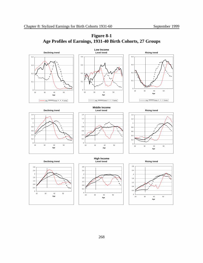
Chapter 8: Stylized Earnings for Birth Cohorts 1931-60 September 1999
268
High IncomeDeclining trend Level trend Rising trend
Middle IncomeDeclining trend Level trend Rising trend
Low IncomeDeclining trend Level trend Rising trend
0
0.1
0.2
0.3
0.4
22 32 42 52
Age
sag linear hump
0
0.1
0.2
0.3
0.4
22 32 42 52
Age
sag linear hump
0
0.1
0.2
0.3
0.4
22 32 42 52
Age
sag linear hump
0
0.2
0.4
0.6
0.8
1
1.2
1.4
22 32 42 52
Age
0
0.2
0.4
0.6
0.8
1
1.2
1.4
22 32 42 52
Age
0
0.2
0.4
0.6
0.8
1
1.2
1.4
22 32 42 52
Age
0
0.4
0.8
1.2
1.6
2
2.4
2.8
22 32 42 52
Age
0
0.4
0.8
1.2
1.6
2
2.4
2.8
22 32 42 52
Age
0
0.4
0.8
1.2
1.6
2
2.4
2.8
22 32 42 52
Age
Figure 8-1Age Profiles of Earnings, 1931-40 Birth Cohorts, 27 Groups

Chapter 8: Stylized Earnings for Birth Cohorts 1931-60 September 1999
269
Percentage distribution. Individuals born in 1931-40, includes years of zero earnings
Low Earnings sag linear humped sag linear humped sag linear humpeddeclining 10.4 2.0 5.4 17.8 6.9 1.2 2.1 10.2 13.7 2.7 8.6 25.0
Trend level 0.6 0.2 1.7 2.6 0.2 0.0 0.2 0.5 1.0 0.4 3.2 4.6
rising 7.3 1.8 5.1 14.3 2.6 0.3 1.0 3.8 11.8 3.3 8.9 24.1
18.3 4.0 12.2 34.6 9.6 1.6 3.3 14.5 26.6 6.4 20.7 53.6
Middle Earnings sag linear humped sag linear humped sag linear humpeddeclining 3.8 4.5 5.5 13.8 6.1 6.3 6.4 18.8 1.6 2.8 4.6 9.0
Trend level 0.6 2.2 1.6 4.5 0.7 1.8 1.0 3.4 0.6 2.7 2.2 5.4
rising 2.2 4.7 6.4 13.3 1.2 1.0 2.0 4.2 3.1 8.2 10.5 21.8
6.6 11.4 13.5 31.5 8.0 9.1 9.4 26.4 5.3 13.6 17.3 36.2
High Earnings sag linear humped sag linear humped sag linear humpeddeclining 1.2 5.1 6.5 12.8 2.5 10.2 12.1 24.9 0.0 0.2 1.2 1.4
Trend level 0.4 10.2 2.3 13.0 0.8 19.3 4.0 24.1 0.1 1.7 0.8 2.5
rising 0.4 5.4 2.3 8.1 0.6 7.1 2.4 10.1 0.2 3.8 2.2 6.2100.0 100.0
2.1 20.7 11.1 33.9 3.9 36.6 18.5 59.1 0.3 5.7 4.2 10.2
ProfileProfile ProfileAll Persons Males Females
Percent of cohort population
Total Male Female Black HispanicNo
degree
High School
DiplomaCollege Degree Qualified Disabled
Low 34.4 13.7 52.9 38.9 44.3 46.5 34.0 25.4 24.1 35.8Middle 29.9 22.8 36.2 40.4 32.4 31.1 32.8 21.1 34.6 42.0High 35.6 63.4 10.9 20.7 23.3 22.4 33.3 53.5 41.3 22.2
Declining 40.0 48.0 32.8 45.1 40.6 50.4 38.6 34.6 37.9 74.1Level 21.4 31.3 12.6 18.9 18.4 19.9 21.4 22.9 23.3 10.6Rising 38.6 20.7 54.6 36.1 41.1 29.6 40.0 42.5 38.8 15.3
Slumped 27.3 21.1 32.7 32.1 30.1 32.2 26.9 23.8 21.1 25.4Linear 38.2 50.8 27.0 34.8 29.7 32.2 37.8 44.6 43.6 22.4Humped 34.6 28.1 40.3 33.1 40.2 35.6 35.3 31.5 35.3 52.2
Profile
Non-disabledHighest Degree Attained
Income Level
Trend
Table 8-1Distribution of Individuals by Age Profile of Earnings, 27 Groups
Table 8-2
Distribution of Individuals by Characteristics and Earnings Profile, 1931-40 Birth Cohort

Chapter 8: Stylized Earnings for Birth Cohorts 1931-60 September 1999
270
have a rising pattern of earnings over their work life, while the most common pattern for men isone of decline. For the profile characteristic, women are somewhat more likely to be at theextremes with a significant hump or slump to their earnings in their middle working years. Blackand Hispanic workers are also scarce in the upper portions of the wage distribution, and blackworkers are somewhat more likely to have declining relative earnings over the work life. Inaddition, workers with low levels of education are far more likely to be in the bottom of thedistribution of earnings and to experience a decline in their relative earnings over their work life. Finally, as illustrated in columns (9) and (10), the distribution of individuals by level and trend ofearnings is very strongly impacted by the exclusion of those who do not have the 40 quarters ofcoverage required to qualify for a pension and the disabled.
1. Boundaries
As shown above in Section II, the separation of earnings patterns by trend (t) and profile(p) was based on a common cutoff value of 1/9th above and below zero for both t and p where A,B, and C are the average earnings in consecutive 10-year subperiods from age 32 to 61. We havetested for the sensitivity to variations in the boundaries. While a widening of the band about zeroincreases the proportion of the sample that falls in the midgroup, there is little effect on thegeneral shape of the earnings profiles. For example, a widening of the boundary from 1/9th to1/6th increases the proportion of the sample in the middle categories by one-third, but it has littlediscernable effect on the shape of the earnings profile. We conclude that the choice of theboundary does not have a major effect on our conclusions about the diversity of earnings patterns,but that we also have little basis for choosing a specific value. The 1/9th was chosen to yieldroughly equal numbers of individuals in each of the three categories of the trend and profile.
2. Non-zero Earnings
The original set of earnings patterns were computed by including the earnings of allindividuals in the category regardless of whether they had earnings in a given year. We alsocomputed a second earnings profile for each group that excluded individuals with earnings of lessthan 0.01 of the average in each specific year. In addition, we can show the proportion ofindividuals in the category that had zero earnings in a given year.
These results are illustrated in Figures 8-2a through 8-2c. In order to reduce the numberof comparisons to a manageable level, the profile dimension is suppressed, and the figures arepresented for 9 categories that separate individuals by the level and trend of the income profile.The profiles are also shown separately for men and women. The exclusion of nonearners in eachyear will obviously result in a higher earnings profile where the magnitude of difference is relatedto the proportion of individuals with zero earnings. But the two earnings profiles remainremarkably similar in appearance. A surprisingly small proportion of the variation in the earningsprofile is related to changes in the proportion of individuals with zero earnings.
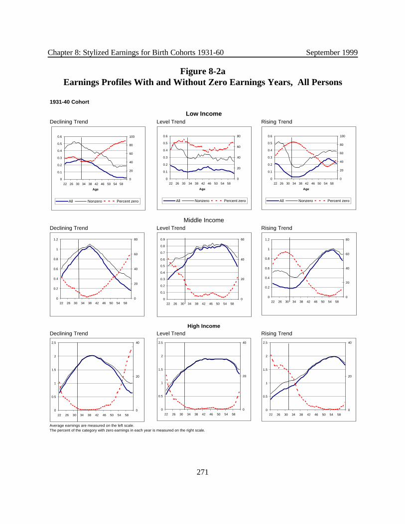
Chapter 8: Stylized Earnings for Birth Cohorts 1931-60 September 1999
271
1931-40 Cohort
Low IncomeDeclining Trend Level Trend Rising Trend
Declining Trend Level Trend Rising Trend
Declining Trend Level Trend Rising Trend
Average earnings are measured on the left scale.The percent of the category with zero earnings in each year is measured on the right scale.
Middle Income
High Income
0
0.1
0.2
0.3
0.4
0.5
0.6
22 26 30 34 38 42 46 50 54 58
Age
0
20
40
60
80
100
All Nonzero Percent zero
0
0.2
0.4
0.6
0.8
1
1.2
22 26 30 34 38 42 46 50 54 58
0
20
40
60
80
0
0.1
0.2
0.3
0.4
0.5
0.6
0.7
0.8
0.9
22 26 30 34 38 42 46 50 54 58
0
20
40
60
0
0.2
0.4
0.6
0.8
1
1.2
22 26 30 34 38 42 46 50 54 58
0
20
40
60
80
0
0.5
1
1.5
2
2.5
22 26 30 34 38 42 46 50 54 58
0
20
40
0
0.5
1
1.5
2
2.5
22 26 30 34 38 42 46 50 54 58
0
20
40
0
0.5
1
1.5
2
2.5
22 26 30 34 38 42 46 50 54 58
0
20
40
0
0.1
0.2
0.3
0.4
0.5
0.6
22 26 30 34 38 42 46 50 54 58
Age
0
20
40
60
80
All Nonzero Percent zero
0
0.1
0.2
0.3
0.4
0.5
0.6
22 26 30 34 38 42 46 50 54 58
Age
0
20
40
60
80
100
All Nonzero Percent zero
Figure 8-2aEarnings Profiles With and Without Zero Earnings Years, All Persons

Chapter 8: Stylized Earnings for Birth Cohorts 1931-60 September 1999
272
1931-40 Cohort
Low IncomeDeclining Trend Level Trend Rising Trend
0
Declining Trend Level Trend Rising Trend
Declining Trend Level Trend Rising Trend
Middle Income
High Income
00.10.20.30.40.50.60.70.8
22 26 30 34 38 42 46 50 54 58
Age
0
20
40
60
80
100
All Nonzero Percent zero 0
0.1
0.2
0.3
0.4
0.5
0.6
0.7
0.8
22 26 30 34 38 42 46 50 54 58
Age
0
20
40
60
80
All Nonzero Percent zero
0
0.1
0.2
0.3
0.4
0.5
0.6
0.7
0.8
22 26 30 34 38 42 46 50 54 58
Age
0
20
40
60
80
100
All Nonzero Percent zero
0
0.2
0.4
0.6
0.8
1
1.2
1.4
22 26 30 34 38 42 46 50 54 580
20
40
60
80
0
0.1
0.2
0.3
0.4
0.5
0.6
0.7
0.8
0.9
1
22 26 30 34 38 42 46 50 54 58
0
20
40
0
0.2
0.4
0.6
0.8
1
1.2
1.4
22 26 30 34 38 42 46 50 54 58
0
20
40
60
0
0.5
1
1.5
2
2.5
22 26 30 34 38 42 46 50 54 580
20
40
0
0.5
1
1.5
2
2.5
22 26 30 34 38 42 46 50 54 580
20
40
0
0.5
1
1.5
2
2.5
22 26 30 34 38 42 46 50 54 58
0
20
40
Figure 8-2bEarnings Profiles With and Without Zero Earnings Years, Men

Chapter 8: Stylized Earnings for Birth Cohorts 1931-60 September 1999
273
1931-40 Cohort
Low IncomeDeclining Trend Level Trend Rising Trend
Declining Trend Level Trend Rising Trend
Declining Trend Level Trend Rising Trend
Middle Income
High Income
0
0.05
0.1
0.15
0.2
0.25
0.3
0.35
0.4
0.45
22 26 30 34 38 42 46 50 54 58
Age
0
20
40
60
80
100
All Nonzero Percent zero
0
0.1
0.2
0.3
0.4
0.5
0.6
22 26 30 34 38 42 46 50 54 58
Age
0
20
40
60
80
100
All Nonzero Percent zero
0
0.1
0.2
0.3
0.4
0.5
0.6
22 26 30 34 38 42 46 50 54 58Age
0
20
40
60
80
100
All Nonzero Percent zero
0
0.1
0.2
0.3
0.4
0.5
0.6
0.7
0.8
0.9
1
22 26 30 34 38 42 46 50 54 58
0
20
40
60
0
0.1
0.2
0.3
0.4
0.5
0.6
0.7
0.8
0.9
22 26 30 34 38 42 46 50 54 58
0
20
40
60
0
0.2
0.4
0.6
0.8
1
1.2
22 26 30 34 38 42 46 50 54 58
0
20
40
60
80
0
0.2
0.4
0.6
0.8
1
1.2
1.4
1.6
1.8
2
22 26 30 34 38 42 46 50 54 58
0
20
40
60
0
0.2
0.4
0.6
0.8
1
1.2
1.4
1.6
1.8
2
22 26 30 34 38 42 46 50 54 58
0
20
40
0
0.2
0.4
0.6
0.8
1
1.2
1.4
1.6
1.8
2
22 26 30 34 38 42 46 50 54 58
0
20
40
60
Figure 8-2cEarnings Profiles With and Without Zero Earnings Years, Women

Chapter 8: Stylized Earnings for Birth Cohorts 1931-60 September 1999
274
There is a very large difference in the frequency of zero earnings years, however, betweenthe low and high-income categories. For the low-income groups, the proportion with zeroearnings in a specific year ranged as high as 80 percent and averages near 60 percent, while thehigh-income earners are distinguished by the stability of their employment rates, with averagenonparticipation rates of less than 10 percent. Furthermore, women are twice as likely as men tohave years of zero earnings between ages 32 and 61, but the rates of non-participation are verycomparable within earnings groups. Because years of zero earnings are more common at thebeginning and end of the work life, they have a significant, but not a dominant, impact on thetrend in earnings.
Since we only have annual information on earnings, it is possible that earnings aredepressed in the year prior to and in the year after a zero-earnings year. Thus, we alsoexperimented with a tabulation that excluded those years as well; but the general shape of eachprofile was largely unaffected.
Finally, we calculated standard deviations for the annual average of the relative wage ineach pattern. Those standard deviations ranged from 0.2 - 0.3 of the economy-wide averagewage in the three low-wage groups to 0.5 - 0.7 for the three high-wage patterns. Thus, thismeasure of variation rises with income, but much less than proportionately. There is also noparticular tendency for the standard errors to rise or fall with increases in age, nor are theresignificant differences by sex.
IV. STYLIZED EARNINGS, 1931-60 BIRTH COHORTS, USING PROJECTED EARNINGS
We applied the methodology described above for earning patterns for the 1931-40 birthcohorts to later cohorts by using the earnings projections presented in Chapter 2 for the yearsafter 1996. The methodology used to classify individuals into specific pattern groups is identicalto that used for the 1931-40 cohorts in Section III of this chapter, but some characteristics of theprojected individual earnings after 1996 suggests that the basic results should be aggregated toabout 9 categories.
1. Classification Into 27 Earnings Patterns
We have calculated the distributions of workers among the 27 categories described abovetogether with the average earnings pattern within each group for ages 22 to 61, the age pattern ofnon-zero earnings, and the percent of individuals in each group with zero earnings in each year.4 The distribution of individuals among the earnings patterns, for all individuals and for men andwomen separately, are summarized in Tables 8-3a through 8-3c and Tables 8-4a through 8-4c.
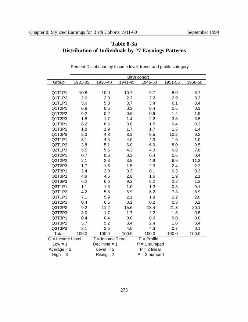
Chapter 8: Stylized Earnings for Birth Cohorts 1931-60 September 1999
275
Percent Distribution by Income level, trend, and profile category
Group 1931-35 1936-40 1941-45 1946-50 1951-55 1956-60
Q1T1P1 10.8 10.0 10.7 9.7 5.0 3.7 Q1T1P2 2.0 2.0 2.3 2.2 2.9 3.2 Q1T1P3 5.6 5.3 3.7 3.4 6.1 8.4 Q1T2P1 0.8 0.5 0.3 0.4 0.5 0.3 Q1T2P2 0.2 0.2 0.6 0.6 1.4 1.9 Q1T2P3 1.8 1.7 1.4 2.2 3.8 3.5 Q1T3P1 8.2 6.6 3.8 1.5 0.4 0.3 Q1T3P2 1.8 1.9 1.7 1.7 1.5 1.4 Q1T3P3 5.3 4.8 8.3 9.5 10.2 9.2 Q2T1P1 3.1 4.5 4.0 4.3 1.6 1.0 Q2T1P2 3.8 5.1 6.0 6.0 8.0 9.5 Q2T1P3 5.5 5.5 4.3 4.3 6.8 7.6 Q2T2P1 0.7 0.6 0.3 0.4 0.6 0.4 Q2T2P2 2.1 2.3 3.8 4.9 8.9 11.3 Q2T2P3 1.7 1.5 1.5 2.3 2.4 2.2 Q2T3P1 2.4 2.0 0.3 0.1 0.3 0.3 Q2T3P2 4.9 4.6 2.8 1.6 1.9 2.1 Q2T3P3 6.2 6.6 9.3 8.2 2.8 1.2 Q3T1P1 1.1 1.3 1.0 1.2 0.3 0.1 Q3T1P2 4.2 5.8 6.9 6.2 7.3 8.9 Q3T1P3 7.1 5.9 2.1 1.8 2.2 2.0 Q3T2P1 0.4 0.5 0.1 0.2 0.3 0.2 Q3T2P2 9.2 11.2 15.6 18.4 21.8 20.1 Q3T2P3 3.0 1.7 1.7 2.2 1.5 0.5 Q3T3P1 0.4 0.4 0.0 0.0 0.0 0.0 Q3T3P2 5.7 5.2 3.4 2.4 1.0 0.4 Q3T3P3 2.1 2.5 4.0 4.3 0.7 0.1
Total 100.0 100.0 100.0 100.0 100.0 100.0 Q = Income Level T = Income Tend P = Profile Low = 1 Declining = 1 P = 1 slumped
Average = 2 Level = 2 P = 2 linear High = 3 Rising = 3 P = 3 humped
Birth cohort
Table 8-3aDistribution of Individuals by 27 Earnings Patterns

Chapter 8: Stylized Earnings for Birth Cohorts 1931-60 September 1999
276
Percent Distribution by Income level, trend, and profile category
Group 1931-35 1936-40 1941-45 1946-50 1951-55 1956-60
Q1T1P1 7.0 6.7 8.4 8.4 6.0 5.6 Q1T1P2 1.3 1.2 1.5 1.5 3.4 4.3 Q1T1P3 2.0 2.1 2.2 3.3 6.7 9.2 Q1T2P1 0.3 0.1 0.1 0.0 0.1 0.2 Q1T2P2 0.0 0.0 0.1 0.0 0.1 0.2 Q1T2P3 0.2 0.2 0.9 1.6 2.1 0.7 Q1T3P1 3.0 2.1 1.2 0.2 0.0 0.1 Q1T3P2 0.1 0.5 0.3 0.1 0.1 0.2 Q1T3P3 1.0 1.0 2.1 1.7 0.6 0.7 Q2T1P1 4.8 7.4 5.6 5.4 2.2 1.6 Q2T1P2 5.5 7.0 8.8 9.8 15.0 17.8 Q2T1P3 6.6 6.2 5.2 6.1 10.3 11.1 Q2T2P1 0.7 0.6 0.1 0.2 0.3 0.2 Q2T2P2 1.9 1.6 1.5 1.0 1.6 1.9 Q2T2P3 1.1 0.9 1.8 3.0 1.7 1.1 Q2T3P1 1.0 1.4 0.1 0.0 0.0 0.0 Q2T3P2 1.0 1.0 0.7 0.3 0.2 0.3 Q2T3P3 2.1 1.8 3.2 3.0 0.4 0.4 Q3T1P1 2.3 2.7 1.9 2.0 0.5 0.2 Q3T1P2 8.6 11.7 13.9 12.6 15.2 18.6 Q3T1P3 13.6 10.8 4.0 3.2 3.8 3.3 Q3T2P1 0.7 0.9 0.2 0.2 0.2 0.2 Q3T2P2 17.7 20.8 27.2 27.4 26.9 21.3 Q3T2P3 5.3 2.8 3.0 4.2 2.0 0.6 Q3T3P1 0.6 0.6 0.0 0.0 0.0 0.0 Q3T3P2 8.8 5.6 2.5 0.7 0.1 0.1 Q3T3P3 2.6 2.2 3.7 4.1 0.5 0.1
Total 100.0 100.0 100.0 100.0 100.0 100.0 Q = Income Level T = Income Tend P = Profile Low = 1 Declining = 1 P = 1 slumped Average = 2 Level = 2 P = 2 linear High = 3 Rising = 3 P = 3 humped
Birth cohort
Table 8-3bDistribution of Individuals by 27 Earnings Patterns, Men

Chapter 8: Stylized Earnings for Birth Cohorts 1931-60 September 1999
277
Percent Distribution by Income level, trend, and profile category
Group 1931-35 1936-40 1941-45 1946-50 1951-55 1956-60
Q1T1P1 14.3 13.1 12.7 10.8 4.0 2.1 Q1T1P2 2.6 2.8 3.1 2.8 2.5 2.3 Q1T1P3 8.9 8.2 5.1 3.5 5.5 7.7 Q1T2P1 1.3 0.8 0.6 0.8 0.8 0.4 Q1T2P2 0.4 0.4 1.0 1.1 2.6 3.3 Q1T2P3 3.3 3.0 1.9 2.7 5.2 5.8 Q1T3P1 13.0 10.7 6.1 2.6 0.7 0.6 Q1T3P2 3.4 3.2 2.9 3.1 2.7 2.3 Q1T3P3 9.5 8.4 13.7 16.3 18.5 16.6 Q2T1P1 1.4 1.9 2.5 3.3 1.0 0.5 Q2T1P2 2.3 3.2 3.6 2.6 1.9 2.3 Q2T1P3 4.5 4.8 3.4 2.8 3.9 4.6 Q2T2P1 0.6 0.6 0.6 0.6 0.9 0.6 Q2T2P2 2.4 3.0 5.8 8.3 15.1 19.4 Q2T2P3 2.3 2.0 1.2 1.7 3.1 3.1 Q2T3P1 3.6 2.6 0.5 0.1 0.5 0.6 Q2T3P2 8.5 7.9 4.6 2.8 3.4 3.7 Q2T3P3 10.0 11.1 14.8 12.7 4.8 2.0 Q3T1P1 0.0 0.0 0.2 0.5 0.1 0.1 Q3T1P2 0.1 0.3 0.8 0.6 0.4 0.6 Q3T1P3 1.1 1.3 0.5 0.6 0.9 0.8 Q3T2P1 0.0 0.2 0.0 0.2 0.4 0.2 Q3T2P2 1.1 2.2 5.3 10.6 17.3 19.1 Q3T2P3 0.8 0.7 0.6 0.4 1.0 0.4 Q3T3P1 0.1 0.2 0.0 0.1 0.0 0.1 Q3T3P2 2.7 4.8 4.1 3.8 1.8 0.6 Q3T3P3 1.7 2.7 4.2 4.5 0.8 0.2
Total 100.0 100.0 100.0 100.0 100.0 100.0 Q = Income Level T = Income Tend P = Profile Low = 1 Declining = 1 P = 1 slumped Average = 2 Level = 2 P = 2 linear High = 3 Rising = 3 P = 3 humped
Birth cohort
Table 8-3cDistribution of Individuals by 27 Earnings Patterns, Women

Chapter 8: Stylized Earnings for Birth Cohorts 1931-60 September 1999
278
Percent Distribution by Income level and trend category
Group 1931-35 1936-40 1941-45 1946-50 1951-55 1956-60 Q1T1 18.3 17.3 16.7 15.4 14.0 15.3 Q1T2 2.8 2.3 2.3 3.3 5.7 5.7 Q1T3 15.3 13.2 13.8 12.7 12.0 10.9 Q2T1 12.4 15.1 14.3 14.6 16.4 18.2 Q2T2 4.5 4.4 5.6 7.6 11.9 13.9 Q2T3 13.4 13.1 12.5 9.9 5.0 3.7 Q3T1 12.5 13.1 10.1 9.2 9.8 11.0 Q3T2 12.5 13.4 17.4 20.8 23.5 20.8 Q3T3 8.2 8.0 7.3 6.7 1.6 0.5 Total 100.0 100.0 100.0 100.0 100.0 100.0
Percent Distribution by Income Level - Thirds
Group 1931-35 1936-40 1941-45 1946-50 1951-55 1956-60Q1 36.5 32.9 32.8 31.3 31.7 31.9 Q2 30.3 32.6 32.3 32.1 33.3 35.8 Q3 33.2 34.5 34.8 36.7 35.0 32.3
Total 100.0 100.0 100.0 100.0 100.0 100.0
Percent Distribution by Trend Characteristic
Group 1931-35 1936-40 1941-45 1946-50 1951-55 1956-60T1 43.2 45.4 41.1 39.1 40.2 44.5 T2 19.9 20.1 25.4 31.6 41.2 40.4 T3 36.9 34.4 33.6 29.2 18.6 15.1
Total 100.0 100.0 100.0 100.0 100.0 100.0
Percent Distribution by Profile Characteristic
Group 1931-35 1936-40 1941-45 1946-50 1951-55 1956-60P1 27.6 26.4 20.6 17.7 8.9 6.5 P2 33.9 38.2 43.0 44.0 54.7 58.8 P3 38.4 35.3 36.4 38.3 36.4 34.7
Total 100.0 100.0 100.0 100.0 100.0 100.0 Q = Income Level T = Income Tend P = Profile Low = 1 Declining = 1 P = 1 slumped
Average = 2 Level = 2 P = 2 linear High = 3 Rising = 3 P = 3 humped
Birth cohort
Birth cohort
Birth cohort
Birth cohort
Table 8-4aSummary Distributions by Earnings Patterns, All Persons

Chapter 8: Stylized Earnings for Birth Cohorts 1931-60 September 1999
279
Percent Distribution by Income level and trend category
Group 1931-35 1936-40 1941-45 1946-50 1951-55 1956-60 Q1T1 10.3 10.0 12.0 13.3 16.1 19.1 Q1T2 0.6 0.3 1.0 1.7 2.3 1.1 Q1T3 4.1 3.6 3.6 1.9 0.6 1.0 Q2T1 16.9 20.6 19.6 21.3 27.6 30.6 Q2T2 3.7 3.2 3.5 4.2 3.6 3.2 Q2T3 4.2 4.2 4.0 3.4 0.6 0.7 Q3T1 24.5 25.2 19.8 17.7 19.5 22.0 Q3T2 23.7 24.5 30.4 31.8 29.1 22.0 Q3T3 12.0 8.3 6.1 4.7 0.6 0.2 Total 100.0 100.0 100.0 100.0 100.0 100.0
Percent Distribution by Income Level - Thirds
Group 1931-35 1936-40 1941-45 1946-50 1951-55 1956-60Q1 15.0 14.0 16.7 16.9 19.1 21.3 Q2 24.8 28.0 27.0 28.9 31.8 34.5 Q3 60.2 58.0 56.3 54.3 49.1 44.3
Total 100.0 100.0 100.0 100.0 100.0 100.0
Percent Distribution by Trend Characteristic
Group 1931-35 1936-40 1941-45 1946-50 1951-55 1956-60T1 51.7 55.9 51.4 52.3 63.2 71.7 T2 27.9 28.0 34.9 37.7 35.1 26.4 T3 20.3 16.1 13.7 10.0 1.8 1.8
Total 100.0 100.0 100.0 100.0 100.0 100.0
Percent Distribution by Profile Characteristic
Group 1931-35 1936-40 1941-45 1946-50 1951-55 1956-60P1 20.5 22.6 17.5 16.4 9.4 8.1 P2 45.0 49.4 56.3 53.4 62.6 64.7 P3 34.5 28.0 26.2 30.2 28.0 27.1
Total 100.0 100.0 100.0 100.0 100.0 100.0 Q = Income Level T = Income Tend P = Profile Low = 1 Declining = 1 P = 1 slumped Average = 2 Level = 2 P = 2 linear High = 3 Rising = 3 P = 3 humped
Birth cohort
Birth cohort
Birth cohort
Birth cohort
Table 8-4bSummary Distributions by Earnings Patterns, Men
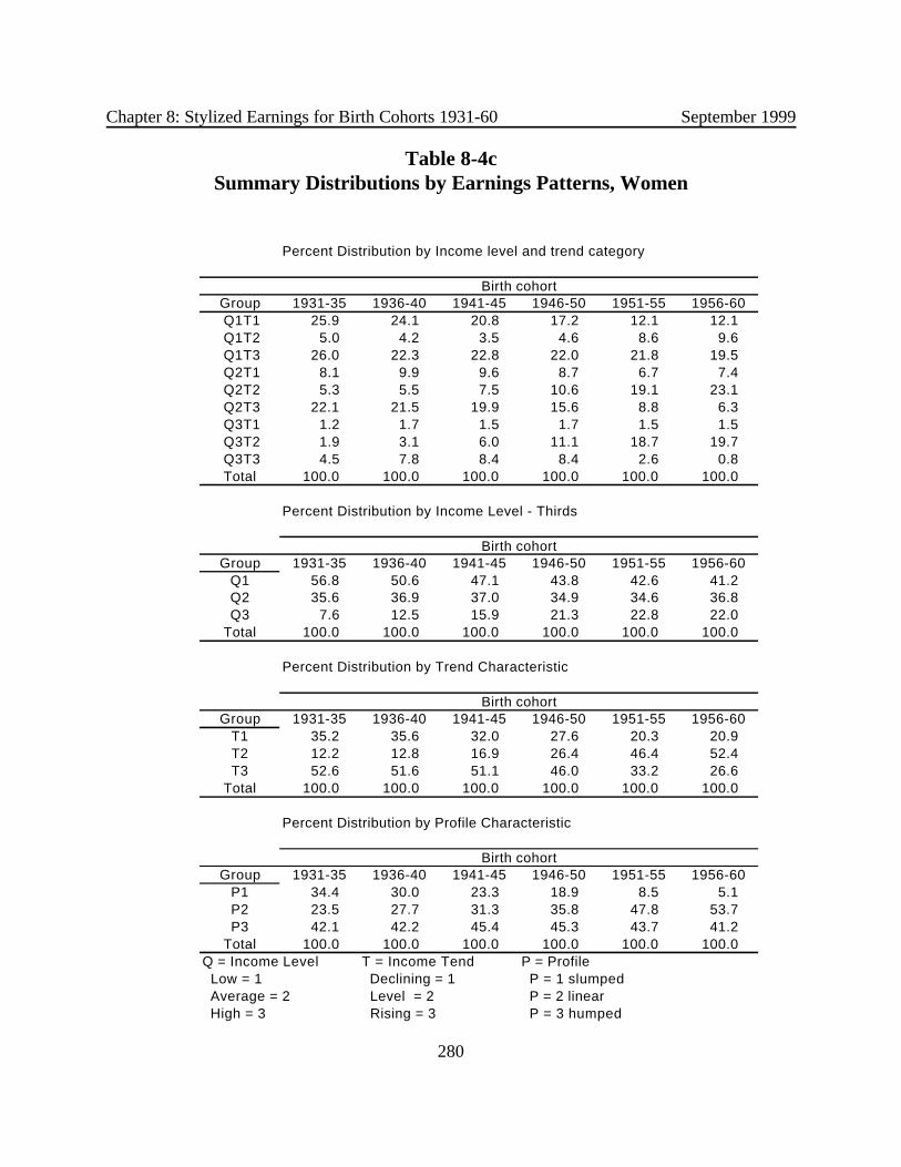
Chapter 8: Stylized Earnings for Birth Cohorts 1931-60 September 1999
280
Percent Distribution by Income level and trend category
Group 1931-35 1936-40 1941-45 1946-50 1951-55 1956-60 Q1T1 25.9 24.1 20.8 17.2 12.1 12.1 Q1T2 5.0 4.2 3.5 4.6 8.6 9.6 Q1T3 26.0 22.3 22.8 22.0 21.8 19.5 Q2T1 8.1 9.9 9.6 8.7 6.7 7.4 Q2T2 5.3 5.5 7.5 10.6 19.1 23.1 Q2T3 22.1 21.5 19.9 15.6 8.8 6.3 Q3T1 1.2 1.7 1.5 1.7 1.5 1.5 Q3T2 1.9 3.1 6.0 11.1 18.7 19.7 Q3T3 4.5 7.8 8.4 8.4 2.6 0.8 Total 100.0 100.0 100.0 100.0 100.0 100.0
Percent Distribution by Income Level - Thirds
Group 1931-35 1936-40 1941-45 1946-50 1951-55 1956-60Q1 56.8 50.6 47.1 43.8 42.6 41.2 Q2 35.6 36.9 37.0 34.9 34.6 36.8 Q3 7.6 12.5 15.9 21.3 22.8 22.0
Total 100.0 100.0 100.0 100.0 100.0 100.0
Percent Distribution by Trend Characteristic
Group 1931-35 1936-40 1941-45 1946-50 1951-55 1956-60T1 35.2 35.6 32.0 27.6 20.3 20.9 T2 12.2 12.8 16.9 26.4 46.4 52.4 T3 52.6 51.6 51.1 46.0 33.2 26.6
Total 100.0 100.0 100.0 100.0 100.0 100.0
Percent Distribution by Profile Characteristic
Group 1931-35 1936-40 1941-45 1946-50 1951-55 1956-60P1 34.4 30.0 23.3 18.9 8.5 5.1 P2 23.5 27.7 31.3 35.8 47.8 53.7 P3 42.1 42.2 45.4 45.3 43.7 41.2
Total 100.0 100.0 100.0 100.0 100.0 100.0 Q = Income Level T = Income Tend P = Profile Low = 1 Declining = 1 P = 1 slumped Average = 2 Level = 2 P = 2 linear High = 3 Rising = 3 P = 3 humped
Birth cohort
Birth cohort
Birth cohort
Birth cohort
Table 8-4cSummary Distributions by Earnings Patterns, Women

Chapter 8: Stylized Earnings for Birth Cohorts 1931-60 September 1999
281
As is evident in Tables 8-3a through 8-3c, the number of individuals in some categories istoo small to provide useful estimates. Tables 8-4a through 8-4c aggregate the earnings patternsacross each of the three characteristics that define an earnings pattern (average earnings, trendand profile) for all individuals, men, and women. The distributions by average earnings remainrelatively stable across the six birth cohorts, but there are significant changes in the distributionsby trend and profile. In particular, it is evident from the distributions by profile at the bottom ofTables 8-4a through 8-4c that the methodology of projecting earnings in Chapter 2 is not able topredict individuals with a sag in earnings during the middle work years. The proportion of allindividuals with a sag pattern (Table 8-4a) falls from 27.6 percent for the 1931-35 birth cohort,where all of the earnings are actual values, to 6.5 percent in the 1956-60 cohort, where earningsare projected after age 40. At the same time the proportion of men with a level earnings pattern(Table 8-4b) rises to over 60 percent in the 1956-60 birth cohort. There is also a substantialdecline in the proportion of men and women with rising earnings patterns as the analysis shiftstoward cohorts with a large proportion of projected earnings. We will return to that issue below.
After consultation with SSA personnel, we have concentrated the remaining portions ofthe analysis on an aggregation of the earnings patterns to nine categories for each sex, whichdistinguish the average level of income and the trend. Spreadsheets that we are supplying to SSAcontain sufficient data to aggregate the basic 27 categories in a variety of alternative ways. Forexample, it is a straightforward process to recreate the 11 patterns that were used in earlier letterreports.
2. Classification Into Nine Earnings Patterns of Level and Trend
The nine earning patterns for men and women are shown for the six birth cohorts inFigures 8-3a through 8-3f. Even with a reduction in the number of groups from 27 to nine, some of the cells are too small to yield stable results. The sample size is provided in Tables 8-4athrough 8-4c. For some male cohorts, groups #2, #3, #6, and #9 are 1 percent of the populationor less. For women the small groups are #7 and #9. Thus, for some purposes, the nine groupswill require further aggregation.
Some important characteristics of the projections of the earnings projections arehighlighted by focusing on the results for the 1931-35 and 1956-60 cohorts. First, as shown inTable 8-4b, there is a sharp decline in the proportion of men with patterns of rising earnings(categories #3, #6, and #9) between the earliest and latest cohort. Similarly, the number of menwith low and level earnings (#2) is small in both cohorts.
Second, comparison of Figures 8-3a and 8-3f shows a substantial compression of therange of the change in earnings over the work life as the analysis moves from the 1931-35 cohortto the 1956-60 cohort. While the average age-earnings patterns for those with level earningstrends are similar between the two cohorts, within the three categories with declining earningspatterns, the magnitude of the drop in earnings over the work life is significantly less for the 1956-

Chapter 8: Stylized Earnings for Birth Cohorts 1931-60 September 1999
282
60 cohort than for the 1931-35 cohort.5 Similarly, the rise in average earnings is smaller for thethree categories with a rising trend.
Likewise, the compression of the range of trend change in earnings and some skewing ofthe distribution of the patterns is evident in Tables 8-4a through 8-4c. As mentioned in the priorsection, there is little net change in the distribution by level of average work life earnings for menand women combined. But there is a sharp rise in the proportion of women in the top third ofthe distribution, from 7.6 percent in the 1931-35 cohort to 22 percent for the 1956-60 cohort. The opposite is true for men where the proportion in the top third of the distribution falls from60.2 to 44.3 percent.
The changes in the distribution of individuals among the categories of trend earnings,shown in the third panel of Tables 8-4a through 8-4c, are also substantial for both men andwomen. For both, there is a sharp falloff in the number with rising earnings pattens, albeit frommuch different proportions in the 1931-35 cohort. For the 1956-60 cohort, only 1.8 percent ofmen and 26.6 percent of women have rising relative earnings over their work life. These comparewith 20.3 and 52.6 percent respectively in the 1931-35 birth cohort. For women, there is also asharp decline in the number with declining relative earnings, a general pattern of compression ofthe distribution of trend changes. In the case of men, however, the sharp fall in the proportionwith a rising trend pattern is matched by an equally large increase in the proportion with decliningrelative earnings over their work life.
To some extent, these changes in the distribution of workers among the earnings patternsreflect trends that we know have been important recently. Women’s earnings are rising faster thatthose for men. However, the tendency toward a compression of the distribution arises from theuse of a limited number of equations to project the central tendency of earnings in Chapter 2. Theage distribution of relative earnings for men and women, implied by the regression coefficients inthe earnings equation from Chapter 2, are shown in Figure 8-4. There are separate earningspatterns for five educational groups and they have been aggregated to the 10-year periods used tocompute the earnings patterns. For men, the earnings patterns are downward sloping over therelevant ages, except for those with some graduate education where the pattern is flat. Forwomen, the opposite is true, earnings rise with age except for the very lowest education group.
While an error term is included in the projections for each individual and year, there willstill be a tendency for the earnings of any subgroup to revert towards the central tendency asexpressed by the regression line. The only identified characteristic that distinguishes individualswith rising earnings patterns from those with falling earnings is their sex. Thus, the group meansare unlikely to display the full range of variation in the trend element, even if the underlyingdistribution of individuals’ earnings does so.

Chapter 8: Stylized Earnings for Birth Cohorts 1931-60 September 1999
283
1931-35 Cohort
Low IncomeDeclining Trend Level Trend Rising Trend
Declining Trend Level Trend Rising Trend
Declining Trend Level Trend Rising Trend
Middle Income
High Income
0
0.05
0.1
0.15
0.2
0.25
0.3
0.35
0.4
0.45
0.5
22 26 30 34 38 42 46 50 54 58
Age
Male Female
0
0.05
0.1
0.15
0.2
0.25
0.3
0.35
0.4
0.45
0.5
22 26 30 34 38 42 46 50 54 58
Age
Male Female
0
0.05
0.1
0.15
0.2
0.25
0.3
0.35
22 26 30 34 38 42 46 50 54 58
Male Female
0
0.2
0.4
0.6
0.8
1
1.2
22 26 30 34 38 42 46 50 54 58
Male Female
0
0.1
0.2
0.3
0.4
0.5
0.6
0.7
0.8
0.9
1
22 26 30 34 38 42 46 50 54 58
Male Female
0
0.2
0.4
0.6
0.8
1
1.2
22 26 30 34 38 42 46 50 54 58
Male Female
0
0.5
1
1.5
2
2.5
22 26 30 34 38 42 46 50 54 58
Male Female
0
0.5
1
1.5
2
2.5
22 26 30 34 38 42 46 50 54 58
Male Female
0
0.5
1
1.5
2
2.5
22 26 30 34 38 42 46 50 54 58
Male Female
Figure 8-3aBasic Earnings Patterns, Male and Female
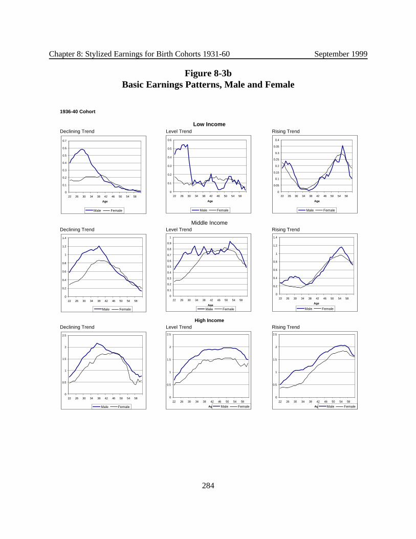
Chapter 8: Stylized Earnings for Birth Cohorts 1931-60 September 1999
284
1936-40 Cohort
Low IncomeDeclining Trend Level Trend Rising Trend
Declining Trend Level Trend Rising Trend
Declining Trend Level Trend Rising Trend
Middle Income
High Income
0
0.1
0.2
0.3
0.4
0.5
0.6
0.7
22 26 30 34 38 42 46 50 54 58
Age
Male Female
0
0.1
0.2
0.3
0.4
0.5
0.6
22 26 30 34 38 42 46 50 54 58
Age
Male Female
0
0.05
0.1
0.15
0.2
0.25
0.3
0.35
0.4
22 26 30 34 38 42 46 50 54 58
Age
Male Female
0
0.2
0.4
0.6
0.8
1
1.2
1.4
22 26 30 34 38 42 46 50 54 58
Male Female
0
0.1
0.2
0.3
0.4
0.5
0.6
0.7
0.8
0.9
1
22 26 30 34 38 42 46 50 54 58
AgeMale Female
0
0.2
0.4
0.6
0.8
1
1.2
1.4
22 26 30 34 38 42 46 50 54 58
Age
Male Female
0
0.5
1
1.5
2
2.5
22 26 30 34 38 42 46 50 54 58
Male Female
0
0.5
1
1.5
2
2.5
22 26 30 34 38 42 46 50 54 58
Age Male Female
0
0.5
1
1.5
2
2.5
22 26 30 34 38 42 46 50 54 58
Age Male Female
Figure 8-3bBasic Earnings Patterns, Male and Female

Chapter 8: Stylized Earnings for Birth Cohorts 1931-60 September 1999
285
1941-45 Cohort
Low IncomeDeclining Trend Level Trend Rising Trend
Declining Trend Level Trend Rising Trend
Declining Trend Level Trend Rising Trend
Middle Income
High Income
0
0.1
0.2
0.3
0.4
0.5
0.6
0.7
22 26 30 34 38 42 46 50 54 58
Age
Male Female
0
0.1
0.2
0.3
0.4
0.5
0.6
22 26 30 34 38 42 46 50 54 58
Age
Male Female
0
0.05
0.1
0.15
0.2
0.25
0.3
0.35
22 26 30 34 38 42 46 50 54 58
Age
Male Female
0
0.2
0.4
0.6
0.8
1
1.2
1.4
22 26 30 34 38 42 46 50 54 58
Male Female
0
0.1
0.2
0.3
0.4
0.5
0.6
0.7
0.8
0.9
1
22 26 30 34 38 42 46 50 54 58
AgeMale Female
0
0.2
0.4
0.6
0.8
1
1.2
22 26 30 34 38 42 46 50 54 58
Age
Male Female
0
0.5
1
1.5
2
2.5
22 26 30 34 38 42 46 50 54 58
Male Female
0
0.5
1
1.5
2
2.5
22 26 30 34 38 42 46 50 54 58
Age Male Female
0
0.5
1
1.5
2
2.5
22 26 30 34 38 42 46 50 54 58
Age Male Female
Figure 8-3cBasic Earnings Patterns, Male and Female

Chapter 8: Stylized Earnings for Birth Cohorts 1931-60 September 1999
286
1946-50 Cohort
Low IncomeDeclining Trend Level Trend Rising Trend
Declining Trend Level Trend Rising Trend
Declining Trend Level Trend Rising Trend
Middle Income
High Income
0
0.1
0.2
0.3
0.4
0.5
0.6
22 26 30 34 38 42 46 50 54 58
Age
Male Female
0
0.05
0.1
0.15
0.2
0.25
0.3
0.35
0.4
0.45
22 26 30 34 38 42 46 50 54 58
Age
Male Female
0
0.05
0.1
0.15
0.2
0.25
0.3
0.35
0.4
22 26 30 34 38 42 46 50 54 58
Age
Male Female
0
0.2
0.4
0.6
0.8
1
1.2
22 26 30 34 38 42 46 50 54 58
Male Female
0
0.2
0.4
0.6
0.8
1
1.2
22 26 30 34 38 42 46 50 54 58
AgeMale Female
0
0.2
0.4
0.6
0.8
1
1.2
1.4
22 26 30 34 38 42 46 50 54 58
Age
Male Female
0
0.2
0.4
0.6
0.8
1
1.2
1.4
1.6
1.8
2
22 26 30 34 38 42 46 50 54 58
Male Female
0
0.5
1
1.5
2
2.5
22 26 30 34 38 42 46 50 54 58
Age Male Female
0
0.5
1
1.5
2
2.5
22 26 30 34 38 42 46 50 54 58
Age Male Female
Figure 8-3dBasic Earnings Patterns, Male and Female
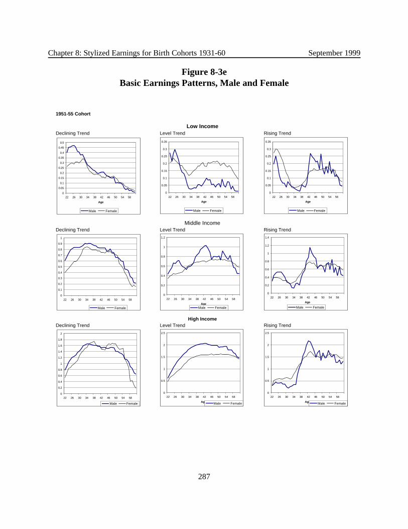
Chapter 8: Stylized Earnings for Birth Cohorts 1931-60 September 1999
287
1951-55 Cohort
Low IncomeDeclining Trend Level Trend Rising Trend
Declining Trend Level Trend Rising Trend
Declining Trend Level Trend Rising Trend
Middle Income
High Income
0
0.05
0.1
0.15
0.2
0.25
0.3
0.35
0.4
0.45
0.5
22 26 30 34 38 42 46 50 54 58
Age
Male Female
0
0.05
0.1
0.15
0.2
0.25
0.3
0.35
22 26 30 34 38 42 46 50 54 58
Age
Male Female
0
0.05
0.1
0.15
0.2
0.25
0.3
0.35
22 26 30 34 38 42 46 50 54 58
Age
Male Female
0
0.1
0.2
0.3
0.4
0.5
0.6
0.7
0.8
0.9
1
22 26 30 34 38 42 46 50 54 58
Male Female
0
0.2
0.4
0.6
0.8
1
1.2
22 26 30 34 38 42 46 50 54 58
AgeMale Female
0
0.2
0.4
0.6
0.8
1
1.2
1.4
22 26 30 34 38 42 46 50 54 58
Age
Male Female
0
0.2
0.4
0.6
0.8
1
1.2
1.4
1.6
1.8
2
22 26 30 34 38 42 46 50 54 58
Male Female
0
0.5
1
1.5
2
2.5
22 26 30 34 38 42 46 50 54 58
Age Male Female
0
0.5
1
1.5
2
2.5
22 26 30 34 38 42 46 50 54 58
Age Male Female
Figure 8-3eBasic Earnings Patterns, Male and Female
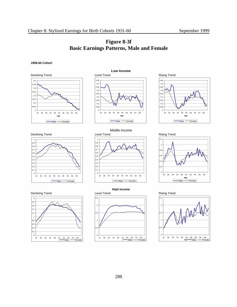
Chapter 8: Stylized Earnings for Birth Cohorts 1931-60 September 1999
288
1956-60 Cohort
Low IncomeDeclining Trend Level Trend Rising Trend
Declining Trend Level Trend Rising Trend
Declining Trend Level Trend Rising Trend
Middle Income
High Income
0
0.05
0.1
0.15
0.2
0.25
0.3
0.35
0.4
22 26 30 34 38 42 46 50 54 58
Age
Male Female
0
0.05
0.1
0.15
0.2
0.25
0.3
0.35
0.4
0.45
22 26 30 34 38 42 46 50 54 58
Age
Male Female
0
0.05
0.1
0.15
0.2
0.25
0.3
0.35
0.4
0.45
22 26 30 34 38 42 46 50 54 58
Age
Male Female
0
0.1
0.2
0.3
0.4
0.5
0.6
0.7
0.8
0.9
1
22 26 30 34 38 42 46 50 54 58
Male Female
0
0.1
0.2
0.3
0.4
0.5
0.6
0.7
0.8
0.9
1
22 26 30 34 38 42 46 50 54 58
Male Female
0
0.2
0.4
0.6
0.8
1
1.2
22 26 30 34 38 42 46 50 54 58
Age
Male Female
0
0.2
0.4
0.6
0.8
1
1.2
1.4
1.6
1.8
2
22 26 30 34 38 42 46 50 54 58Male Female
0
0.5
1
1.5
2
2.5
22 26 30 34 38 42 46 50 54 58Male Female
0
0.5
1
1.5
2
2.5
22 26 30 34 38 42 46 50 54 58Age Male Female
Figure 8-3fBasic Earnings Patterns, Male and Female
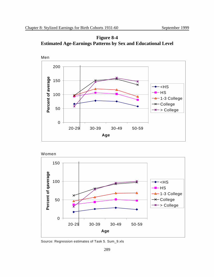
Chapter 8: Stylized Earnings for Birth Cohorts 1931-60 September 1999
289
Men
Women
Source: Regression Estimates of Task 5.
Source: Regression estimates of Task 5. Sum_9.xls
0
50
100
150
200
20-29 30-39 30-49 50-59
Age
Per
cen
t o
f av
erag
e
<HSHS1-3 CollegeCollege> College
0
50
100
150
20-29 30-39 30-49 50-59
Age
Per
cen
t o
f q
aver
age
<HSHS1-3 CollegeCollege> College
Figure 8-4Estimated Age-Earnings Patterns by Sex and Educational Level

Chapter 8: Stylized Earnings for Birth Cohorts 1931-60 September 1999
290
However, there also appears to be an element of bias in the projections because we wouldexpect a substantial number of women to continue to have a rising age-earnings pattern. Insteadthe pace of decline in the number of both men and women in the rising trend categories of Tables8-4b and 8-4c accelerates with the 1951-55 birth cohort. One possible reason for this is that theearnings regressions reported in Chapter 2 were originally developed with historical data thatincluded the earnings of the disabled. The projections are based on those regressions. However,in a later stage of the projections the earnings of those who are predicted to become disabled areconverted to zero with the onset of disability. This results in a downward bias in the mean rate ofearnings growth for the population as a whole, because the disabled are included in the samplethat predicts earnings of the non-disabled. As discussed in Chapter 2, however, the bias may bemodest to the extent that the disabled workers whose earnings are zeroed out had below averageprojected earnings.
Finally, the methodology used to project earnings in Chapter 2 will project an appropriatenumber of workers with low earnings, but it does not predict zero earnings. This is not a problemfor the earnings patterns themselves, but it may have some influence on the decomposition of thenine earnings patterns into an age-earnings pattern of those with positive earnings and theproportion of individuals with zero earnings at a given age. However, in constructing the averageof nonzero earnings, we used a cutoff value of 0.01 of the average wage relative than absolutezero. Table 8-5 shows the average proportion of ‘zero’ earnings years in the 1956-60 cohortcompared with the historical data of the 1931-35 cohort. There is a decline in the proportion ofzero-earnings years, but it is concentrated among low-earning women and seems quite in keepingwith their rising pattern of labor force participation.
3. Earnings Patterns of Married Couples
The nine earnings patterns for men and women have also been matched in a set of couplesfiles. There are a total of 12 files, six cohorts for both men and women, with nine tables in eachfile corresponding to the nine earnings patterns. The structure of those files is shown in Table 8-6. The less-censored earnings of line 2 are the same as the age-earnings patterns reported insection B, and taxable earnings are reported on line 3. The two measures of earnings are the sameafter 1989 when the taxable earnings ceiling was indexed to the economy-wide average wage. The proportion of individuals with sufficient taxable earnings to qualify for the basic pension andthe Primary Insurance Amount (PIA) are reported on lines 4 and 5. The PIA is the average of theindividual PIAs, and it is computed on the basis of the relative earnings up to age 61; but it usesthe level of earnings and the ‘bend points” of 1996.
Lines 7-12 show the distribution of the respondents by marital status, and the PIA of thespouse. The distribution of the spouses’ and their PIAs among the nine age-earnings patterns isreported on lines 14-23. Some spouses are not in the universe if their birth year was outside therange of 1926-65 or they had no taxable earnings. The percentage of individuals in the groupsurviving at each age from 63 to 110 is shown on line 26.

Chapter 8: Stylized Earnings for Birth Cohorts 1931-60 September 1999
291
Pattern1931-35 1956-60 1931-35 1956-60 1931-35 1956-60
Q1T1 64 47 61 53 65 39Q1T2 61 20 37 52 64 17QiT3 58 26 67 45 57 25Q2T1 23 13 23 12 22 19Q2T2 7 3 4 11 8 2Q2T3 21 8 24 24 20 7Q3T1 8 5 8 4 13 12Q3T2 2 1 2 1 3 0Q3T3 5 5 3 14 10 3Total 28 14 25 24 29 14
based on a cuttoff of 0.01 of the economy-wide average wage
Total Men Women
Table 8-5Frequency of Zero Earnings Year, by Sex,
Birth Cohort, and Earnings Pattern
Annual average of percentages, ages 31-61

Chapter 8: Stylized Earnings for Birth Cohorts 1931-60 September 1999
292
AGEMEN GROUP Q1T1 22 23 24 25 26 ..
LESS CENSORED AVERAGE INDEXED EARNINGS 0.29105648 0.357962 0.407357 0.425066 0.436204 ..AVERAGE INDEXED TAXABLE EARNINGS 0.2856392 0.340941 0.39583 0.40325 0.413025 ..Percent with PIA 71.7Average PIA $501.02
Marital Status at Age 62
Unweighted Number of
Observations
Weighted Number of
Observations
Percent of Spouses with
PIA
Average PIA of the Spouse
TOTAL 275 458 60.9 $578.20MARRIED 204 337 59.6 $584.84WIDOWED 15 26 69.9 $601.35DIVORCED 23 41 66.1 $512.90OTHER 13 21 (NA) (NA)NEVER MARRIED 20 34 (NA) (NA)
Spouse's Stylized Group
Unweighted Number of
Observations
Weighted Number of
Observations
Percent of Spouses with
PIA
Average PIA of the Spouse
GROUP Q1T1 69 114 51.6 $362.67GROUP Q1T2 14 23 45.2 $440.03GROUP Q1T3 60 99 59.3 $353.45GROUP Q2T1 19 33 100.0 $685.40GROUP Q2T2 8 13 100.0 $723.25GROUP Q2T3 28 47 100.0 $761.38GROUP Q3T1 0 0 0.0 $0.00GROUP Q3T2 5 10 100.0 $1,155.99GROUP Q3T3 10 15 100.0 $1,092.71Not in Universe 62 105
458 AGE63 64 65 66 67 ..
PERCENT SURVIVING TO SPECIFIED AGE 97.322 93.984 88.466 85.377 83.100
The 31 to 35 year cohortWeighted observations are shown in thousands.Average PIA of the group is based on those with nonzero aime at age 62.Average PIA of spouse is based on those with nonzero aime at age 62.Aime converted to 1996 dollars before computation of PIA.Universe - Persons of Specified Sex Reaching Age 62 in their life and with nonzero earnings during the ages 31 to 62.Not in Universe - No spouse at age 62 or spouse without earnings during the Ages 32-61.Persons with disability onset before age 62 are included.
Table 8-6Contents of the Couples Files, 1931-35 Cohort

Chapter 8: Stylized Earnings for Birth Cohorts 1931-60 September 1999
293
Table 8-7 provides a summary of the extent of marital matching by income level for the 6birth cohorts using both men and women as the reference persons. While there is some tendencyfor individuals to have spouses in the same income group, it is largely overwhelmed by thedifferences in income levels between the two sexes. That is, while the proportion of high-incomemen married to high-income women rises for later birth cohorts, that is largely due to the generaltendency for women to move higher in the overall income distribution relative to men.6 However,there is a very strong tendency for women, even those in the top income group, to marry menwith a higher income.
Tables 8-8a and 8-8b report the PIA for married individuals, their spouse’s PIA, and thecombined total for each of the 9 earnings patterns for both sexes and the six birth cohorts. PIAsare reported only for those with a nonzero AIME at age 62. Because the PIAs are estimated onthe basis of 1996 economic conditions, the average PIAs of each group are relatively constantacross the six cohorts. However, the combined PIAs of couples distributed by the males’ income(Table 8-8a) is rising for later cohorts because the spouse is moving into the higher incomegroups. No such pattern is evident for women (Table 8-8b), but the combined PIA is much higherfor each group when women are used as the reference group because of their tendency to havespouses with a higher work-life income and PIA. Finally, the combined values only includeindividual and spouses who qualify for their own pension, i.e., have a PIA.
Tables 8-9a and 8-9b report the proportions of individuals in each group at age 62 whosurvive to various later ages, for each sex and the six birth cohorts. They show the expectedpattern of a higher proportion of women than men surviving to a given age. There is also apositive correlation between survivorship and income level. However, the correlation withaverage work life income is less than one might expect because of a low correlation between themeasure of permanent income constructed from SIPP data and our measure of work life incomewhich is a 30-year average of earnings. In addition, some of the cells are too small to yieldreliable results.

Chapter 8: Stylized Earnings for Birth Cohorts 1931-60 September 1999
294
Men
Percentages of Marital Matching of Income Levels, by Age Cohort
Age Cohort1931-1935 1936-1940 1941-1945 1946-1950 1951-1955 1956-1960
Low Low 68% 62% 60% 54% 53% 52%Low Middle 26% 30% 32% 30% 31% 33%Low High 7% 8% 8% 16% 15% 15%Middle Low 58% 54% 51% 47% 41% 41%Middle Middle 36% 37% 38% 38% 41% 44%Middle High 6% 10% 10% 16% 17% 16%High Low 57% 48% 47% 45% 42% 40%High Middle 33% 37% 34% 33% 34% 35%High High 10% 15% 19% 22% 24% 24%
Women
Percentages of Marital Matching of Income Levels, by Age Cohort
Age Cohort1931-1935 1936-1940 1941-1945 1946-1950 1951-1955 1956-1960
Low Low 14% 15% 17% 20% 21% 20%Low Middle 28% 31% 31% 28% 33% 36%Low High 58% 54% 52% 52% 45% 43%Middle Low 11% 12% 13% 14% 15% 14%Middle Middle 24% 28% 31% 32% 38% 28%Middle High 65% 60% 56% 53% 47% 58%High Low 10% 10% 9% 11% 12% 17%High Middle 17% 23% 18% 22% 26% 16%High High 73% 67% 72% 67% 62% 67%
Source: spousesumm.xls
Man's Income Level:
Wife's Income Level
Woman's Income Level:
Husband's Income Level
Table 8-7Marital Matching of Income Levels, Cohorts 1931-60

Chapter 8: Stylized Earnings for Birth Cohorts 1931-60 September 1999
295
Average PIA - Men
1931-1935 1936-1940 1941-1945 1946-1950 1951-1955 1956-1960Low Declining $501 $536 $564 $541 $513 $499Low Level $498 $447 $487 $499 $456 $485Low Increasing $407 $394 $417 $399 $359 $422
Middle Declining $829 $857 $864 $866 $847 $822Middle Level $812 $812 $819 $849 $837 $842Middle Increasing $729 $734 $749 $764 $712 $748High Declining $1,115 $1,170 $1,184 $1,189 $1,184 $1,169High Level $1,184 $1,235 $1,277 $1,294 $1,302 $1,311High Increasing $1,193 $1,198 $1,199 $1,182 $1,111 $1,200
1931-1935 1936-1940 1941-1945 1946-1950 1951-1955 1956-1960Low Declining $578 $599 $600 $655 $623 $623Low Level $625 $548 $597 $732 $667 $689Low Increasing $565 $589 $614 $662 $646 $760
Middle Declining $605 $634 $630 $675 $677 $679Middle Level $586 $607 $643 $679 $734 $739Middle Increasing $581 $625 $695 $628 $777 $632High Declining $595 $667 $685 $708 $715 $718High Level $645 $698 $728 $742 $743 $765
High Increasing $612 $692 $794 $727 $627 $774
1931-1935 1936-1940 1941-1945 1946-1950 1951-1955 1956-1960Low Declining $1,079 $1,135 $1,165 $1,196 $1,137 $1,123Low Level $1,123 $994 $1,084 $1,232 $1,123 $1,174Low Increasing $972 $983 $1,031 $1,061 $1,005 $1,182
Middle Declining $1,434 $1,492 $1,494 $1,541 $1,524 $1,500Middle Level $1,397 $1,420 $1,462 $1,528 $1,571 $1,581Middle Increasing $1,311 $1,359 $1,444 $1,392 $1,488 $1,380High Declining $1,710 $1,837 $1,869 $1,897 $1,899 $1,887High Level $1,829 $1,932 $2,005 $2,036 $2,045 $2,076High Increasing $1,805 $1,890 $1,993 $1,908 $1,739 $1,974
Source: Piasum.xls
Income Third
Income Trend
Age CohortAverage PIA - Total
Income Third
Income Trend
Age CohortAverage PIA - Wives
Income Third
Income Trend
Age Cohort
Table 8-8aAverage Primary Insurance Amount, Men, 1931-60

Chapter 8: Stylized Earnings for Birth Cohorts 1931-60 September 1999
296
Average PIA - Women
1931-1935 1936-1940 1941-1945 1946-1950 1951-1955 1956-1960Low Declining $410 $422 $419 $453 $468 $435Low Level $407 $402 $385 $404 $414 $377Low Increasing $398 $390 $391 $384 $350 $343
Middle Declining $696 $718 $745 $777 $811 $797Middle Level $717 $742 $748 $747 $742 $751Middle Increasing $696 $698 $708 $707 $701 $729High Declining $1,060 $1,110 $1,153 $1,164 $1,200 $1,205High Level $1,084 $1,119 $1,157 $1,182 $1,178 $1,179High Increasing $1,074 $1,102 $1,122 $1,140 $1,125 $1,136
1931-1935 1936-1940 1941-1945 1946-1950 1951-1955 1956-1960Low Declining $965 $969 $1,001 $981 $955 $893Low Level $945 $970 $1,007 $994 $956 $946Low Increasing $999 $1,023 $1,038 $1,072 $1,059 $1,038
Middle Declining $995 $981 $1,014 $1,032 $1,008 $935Middle Level $988 $964 $999 $1,026 $1,009 $958Middle Increasing $1,014 $1,047 $1,072 $1,063 $1,064 $1,059High Declining $1,044 $1,066 $1,168 $1,102 $1,117 $1,146High Level $1,033 $1,050 $1,098 $1,087 $1,093 $1,064
High Increasing $1,070 $1,070 $1,143 $1,153 $1,073 $1,157
1931-1935 1936-1940 1941-1945 1946-1950 1951-1955 1956-1960Low Declining $1,375 $1,391 $1,420 $1,434 $1,423 $1,329Low Level $1,352 $1,373 $1,392 $1,397 $1,370 $1,323Low Increasing $1,397 $1,414 $1,429 $1,456 $1,409 $1,382
Middle Declining $1,691 $1,699 $1,759 $1,809 $1,819 $1,731Middle Level $1,705 $1,706 $1,747 $1,773 $1,751 $1,709Middle Increasing $1,711 $1,744 $1,780 $1,771 $1,765 $1,788High Declining $2,105 $2,176 $2,320 $2,266 $2,317 $2,351High Level $2,117 $2,169 $2,255 $2,269 $2,271 $2,242High Increasing $2,144 $2,172 $2,265 $2,294 $2,198 $2,293
Source: Piasum.xls
Income Trend
Age CohortIncome Third
Income Trend
Age Cohort
Average PIA - Total
Income Third
Income Trend
Age Cohort
Average PIA - Husbands
Income Third
Table 8-8bAverage Primary Insurance Amount, Women, 1931-60

Chapter 8: Stylized Earnings for Birth Cohorts 1931-60 September 1999
297
Percent of Men Surviving to Age 65
Age CohortIncome Level: 1931-1935 1936-1940 1941-1945 1946-1950 1951-1955 1956-1960
Low Decreasing 88.466 94.162 93.329 93.445 92.968 91.518Level 67.532 100.000 85.516 93.416 93.945 97.547
Increasing 89.889 94.798 90.796 95.151 91.253 96.096Middle Decreasing 89.395 94.187 94.674 93.039 95.210 95.012
Level 91.814 86.576 93.503 92.274 96.943 96.530Increasing 97.245 95.981 93.956 91.518 100.000 96.058
High Decreasing 91.962 93.565 95.163 95.312 95.933 94.846Level 92.494 94.210 94.155 95.350 95.435 95.932
Increasing 93.457 94.844 92.858 98.585 92.744 100.000
Percent of Men Surviving to Age 70
Age CohortIncome Level: 1931-1935 1936-1940 1941-1945 1946-1950 1951-1955 1956-1960
Low Decreasing 72.264 80.412 81.742 80.549 77.707 78.663Level 62.173 100.000 71.033 80.864 78.265 83.966
Increasing 68.745 81.674 81.870 80.825 91.253 80.400Middle Decreasing 75.322 81.598 84.277 81.434 84.525 83.783
Level 75.861 76.418 82.658 76.975 88.209 86.802Increasing 83.478 82.151 83.708 81.597 92.594 80.631
High Decreasing 78.779 82.262 84.487 86.318 84.892 85.392Level 79.981 83.893 84.042 86.462 85.302 87.444
Increasing 81.192 85.109 82.291 90.579 86.552 92.999
Percent of Men Surviving to Age 75Age Cohort
Income Level: 1931-1935 1936-1940 1941-1945 1946-1950 1951-1955 1956-1960
Low Decreasing 58.180 65.832 63.203 63.985 66.271 62.530Level 51.111 90.938 44.959 63.952 66.413 74.165
Increasing 58.177 67.955 70.469 68.590 73.523 69.688
Middle Decreasing 61.314 65.623 68.436 68.125 69.874 70.781Level 65.531 63.338 66.589 62.110 67.779 72.132
Increasing 62.204 65.449 72.891 63.555 78.691 65.524High Decreasing 65.945 70.298 70.513 74.527 72.157 72.063
Level 67.879 72.166 70.494 73.575 73.723 73.423Increasing 68.663 75.019 68.607 79.609 75.270 92.999
Source: life3xp.xls
Table 8-9aSurvival After Age 62, Men, 1931-60 Cohorts

Chapter 8: Stylized Earnings for Birth Cohorts 1931-60 September 1999
298
Percent of Women Surviving to Age 65
Age CohortIncome Level: 1931-1935 1936-1940 1941-1945 1946-1950 1951-1955 1956-1960
Low Decreasing 93.154 97.628 97.237 98.018 97.311 96.736Level 95.849 98.110 96.066 96.524 97.466 97.385
Increasing 95.948 96.481 97.292 98.478 97.703 97.739Middle Decreasing 94.272 98.179 97.297 97.709 98.630 97.114
Level 94.158 98.193 98.058 97.446 98.429 97.986Increasing 95.456 98.456 97.596 97.945 97.750 99.047
High Decreasing 96.280 98.406 95.901 97.722 96.712 97.375Level 97.258 95.789 97.309 98.477 98.479 98.194
Increasing 97.373 97.625 98.072 98.553 98.357 100.000
Percent of Women Surviving to Age 70
Age CohortIncome Level: 1931-1935 1936-1940 1941-1945 1946-1950 1951-1955 1956-1960
Low Decreasing 87.032 93.021 92.628 91.584 91.893 90.970Level 89.378 93.993 90.195 90.289 92.463 92.209
Increasing 88.825 92.057 91.793 93.492 91.763 94.061Middle Decreasing 89.312 95.225 93.417 93.453 95.389 93.499
Level 83.241 89.858 93.972 92.064 92.743 93.476Increasing 91.467 92.783 92.087 93.911 91.350 95.135
High Decreasing 96.280 92.478 94.274 93.647 90.844 96.012Level 90.778 91.848 93.230 94.693 94.716 95.439
Increasing 94.249 92.385 95.647 94.942 96.234 97.505
Percent of Women Surviving to Age 75Age Cohort
Income Level: 1931-1935 1936-1940 1941-1945 1946-1950 1951-1955 1956-1960
Low Decreasing 78.358 85.176 84.636 84.877 83.241 83.271Level 85.074 90.363 80.900 82.551 84.927 85.887
Increasing 80.873 85.820 86.117 87.111 85.266 88.092Middle Decreasing 82.474 86.945 85.848 87.284 89.092 86.665
Level 78.587 83.846 85.304 85.405 85.730 88.191Increasing 83.633 86.467 84.359 87.629 84.455 91.188
High Decreasing 86.940 85.025 88.225 90.058 81.305 93.849Level 80.760 89.157 84.813 91.121 89.585 90.371
Increasing 89.102 86.160 90.546 88.328 93.636 97.505Source: life3xp.xls
Table 8-9bSurvival After Age 62, Women, 1931-60 Cohorts

Chapter 8: Stylized Earnings for Birth Cohorts 1931-60 September 1999
299
APPENDIX A COMPARING MINT STYLIZED PROFILES WITH TRADITIONAL SOCIAL SECURITY WAGE PROFILES
I. INTRODUCTION
This Appendix presents computations comparing the present value of OASI lifetimebenefits and the wealth that workers with stylized earnings patterns would accrue at retirement ifthey could invest employee and employer OASI contributions in defined contribution accountswith alternative assumed rates of return. It also computes the internal rate of return on OASIcontributions. These calculations are performed for workers with the stylized earnings patternsreported in this chapter and the results are compared with the same calculations for workers withthe traditional Social Security “Low,” “Average,” and “Maximum” wage profiles.
As a note to the reader, the terms “stylized earners,” “profiles,” and “wage earners” areused interchangeably in this appendix.
II. STYLIZED EARNINGS PATTERNS
Traditionally, Social Security has developed estimates of the returns to Social Security onthe basis of three stylized earnings patterns. The maximum-income group represents those whohad earnings at the maximum taxable amount in every year. The middle group is represented bysomeone who earns at the average taxable earnings amount in every year, and the low-incomegroup represents those who earn at 45 percent of this average amount.
The MINT project has generated more representative stylized profiles across thepopulation, facilitating comparison with the more traditional stylized Social Security earners onsuch issues as accumulated wealth and rates of return. Among the various stylized patterns, it isalso possible to trace out how the pattern of earnings over time might affect the accumulation ofpension wealth in a reformed system that might include individual accounts.
We use 9 stylized earnings patterns for both men and women born between 1931 and1960 inclusive. The profiles categorize workers based on whether their lifetime earnings are low,middle, or high and whether their average earnings between ages 31-40 and 51-60 are decreasing,level, or increasing. Table 8-A-1 shows the distribution of earnings patterns for the

Chapter 8: Stylized Earnings for Birth Cohorts 1931-60 September 1999
300
Table 8-A-1Mint Wage Profile Descriptions and Sample Weights
for 1935 Birth Cohort
MaleWageProfile
Description MaleSample
Size
FemaleSample
Size
PercentDistribution
(Two-Earner)Spouse’sProfile
Male Female
1 Low income, decreasing 458 1,218 10.3 25.9 1
2 Low income, level 25 235 0.6 5.0 3
3 Low income, increasing 183 1,221 4.1 26.0 3
4 Middle income, decreasing 753 382 16.9 8.1 1
5 Middle income, level 164 251 3.7 5.3 3
6 Middle income, increasing 187 1,039 4.2 22.1 6
7 High income, decreasing 1,092 55 24.5 1.2 3
8 High income, level 1,055 90 23.7 1.9 3
9 High income, increasing 536 213 12.0 4.5 3
Totals 4,453 4,704 100.0 100.0 —
The table shows that profiles 1, 4, 7, and 8 represent 75 percent of the 1931-35 sample ofmale earners. (For the 1951-55 sample, these same four profiles comprise 92 percent of maleearners).
Computations of the MINT and SSA wage profile characteristics discussed in thisappendix are driven by the following assumptions.
• We took 5-year averages of the data so that we are modeling 6 cohorts: 1931-35, 1936-40, 1941-45, 1946-50, 1951-55, and 1956-60.
• Earnings are measured as multiples of the Social Security average wage in each year andthen aligned by the age of the individual. The Social Security “Low” and “Average”profiles are constant multiples of the average wage in every year of a worker’s career,while the MINT profile multiples vary from year to year. The “Average” or middle SocialSecurity profile is always 1, corresponding to the average wage in that year; the “Low”profile is always 0.45 times the average wage; the “Maximum” profile is the ratio of thetaxable maximum to the average wage in a given year.

Chapter 8: Stylized Earnings for Birth Cohorts 1931-60 September 1999
301
• The actual shape of the age-earnings patterns change from cohort to cohort along with thedistribution of individuals among the nine patterns, although the criteria for classifyingpersons among the groups remains the same. The general trend is for relative earnings toincrease over time, but there is wide diversity with considerable numbers of persons whoseearnings decline with age in the lower income groups.
• Workers are assumed to pay both the employee’s and employer’s share of Social Securitytaxes; that is, employers will in practice transfer the burden of such taxes to workers in theform of reduced wages.
• All persons are assumed to retire at age 65. Hence, those retiring in 2003 and later seetheir monthly benefits actuarially reduced based on the schedule in current law.
• Couples are assumed to be the same age and have two children, born when parents areaged 25 and 30. This factor is important because our model includes all possible,expected streams of OASI survivors’, spousal, or workers’ benefits that can be receivedin each year of a worker’s career and retirement, in its estimates of lifetime socialsecurity benefits.
• Our computations employ 1998 OASDI Trustees economic assumptions and 1998 birthcohort life tables from the Office of the Actuary at the Social Security Administration.
III. PRINCIPAL FINDINGS
Our principal findings, using the nine stylized earnings patterns described above, are thefollowing:
• For low and middle earners, Social Security's traditional stylized patterns generallyrepresent workers with higher career earnings than is representative in the population as awhole. Thus, Social Security's low earner is closer to someone with between low andaverage career earnings, its person with average earnings is closer to someone betweenaverage and high earnings.
• Mainly because of these differences, we find that profiles of low and average earnerscomputed in MINT have lower Social Security retirement benefits, but receive higherinternal rates of return from Social Security than the traditional stylized earner in SocialSecurity.
• The traditional measure of earnings in Social Security assumes that a worker earns thesame wage, relative to the average wage in the economy, every year. That is, they start,stop, and stay at their highest and lowest wage, relative to the economy. He or she is also

Chapter 8: Stylized Earnings for Birth Cohorts 1931-60 September 1999
302
never out of the labor force for the year. Implicitly, then, Social Security's stylizedearnings pattern takes the average wage for all earners in a given year rather than theaverage wage for all people who participate in Social Security, whether they work or notin a given year.
• As a consequence, given normal earnings patterns, the replacement rate defined as thepercentage of peak year’s earnings replaced by Social Security is much lower for theMINT representative worker than for the SSA stylized patterns with level earnings. Theprimary insurance amount as a percent of the economy-wide average wage is also lowerfor the MINT workers than the SSA workers. However, the primary insurance amount asa percent of the average earnings (indexed) is higher for the MINT workers, especially forlow earners and one-earner couples, than for their SSA counterparts. The higherreplacement rate for MINT workers compared with their SSA counterparts reflects theinteraction of their lower earnings with the redistributive benefit formula in SocialSecurity.
• How one fares with an individual account vis-a-vis the Social Security benefit formuladepends upon the rate of return in the account and the variance in lifetime earningspatterns. At higher rates of return especially, those whose lifetime earnings come earlier inlife fare relatively better under individual accounts than do those whose earnings comelater in life. We see this effect in contrasting the social security stylized earners whoreceive their peak wage from their starting year and hence make larger contributionsearlier on that accumulate more interest over time than the MINT earners, who experiencemore typical hump shaped earnings patterns and, in particular, have much lower earningsin the earliest years of their careers.
IV. DETAILED DISCUSSION OF RESULTS
In the tables below, we first display a comparison of earnings and social security benefitsfor representative MINT and SSA earners. We then compare lifetime net benefits under SocialSecurity and a system of individual accounts for different family types and earnings profiles. Thelast group of tables shows internal rates of return and replacement rates under the current SocialSecurity benefit formula for different types of workers, again using both the MINT and SSAprofiles.
Table 8-A-2 shows annualized average indexed monthly earnings (AIME) for the SSA andMINT profiles in year 2000 dollars. SSA profiles enjoy significantly higher average earnings thantheir MINT counterparts. In most cases, SSA profiles receive higher wages than MINT profilesin every year of work.
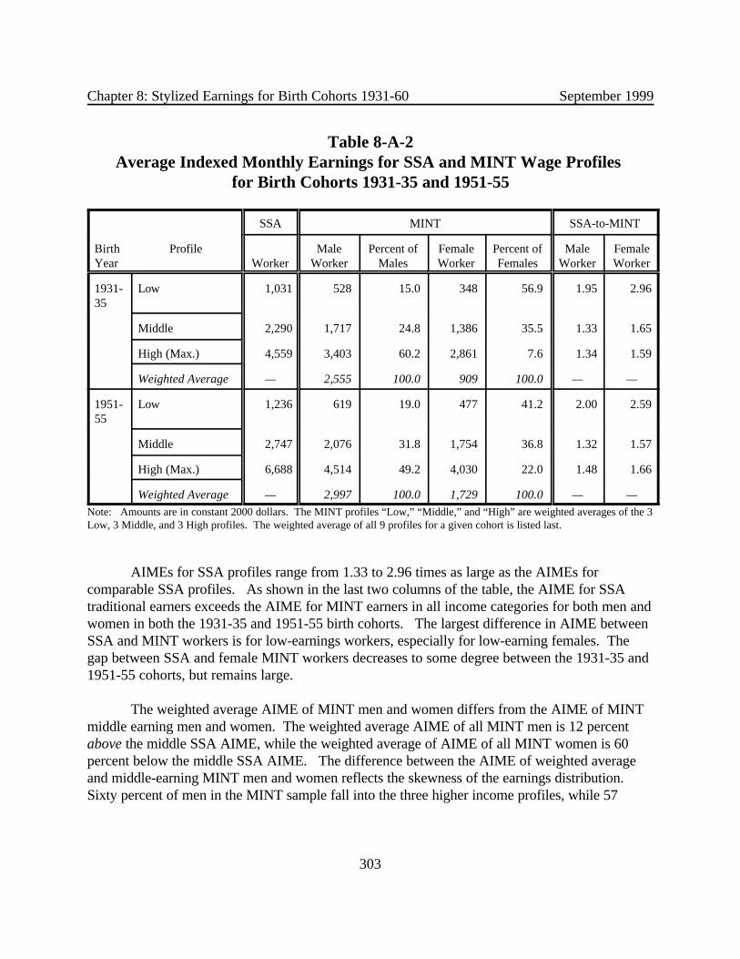
Chapter 8: Stylized Earnings for Birth Cohorts 1931-60 September 1999
303
Table 8-A-2Average Indexed Monthly Earnings for SSA and MINT Wage Profiles
for Birth Cohorts 1931-35 and 1951-55
SSA MINT SSA-to-MINT
BirthYear
Profile Worker
MaleWorker
Percent ofMales
FemaleWorker
Percent ofFemales
MaleWorker
FemaleWorker
1931-35
Low 1,031 528 15.0 348 56.9 1.95 2.96
Middle 2,290 1,717 24.8 1,386 35.5 1.33 1.65
High (Max.) 4,559 3,403 60.2 2,861 7.6 1.34 1.59
Weighted Average — 2,555 100.0 909 100.0 — —
1951-55
Low 1,236 619 19.0 477 41.2 2.00 2.59
Middle 2,747 2,076 31.8 1,754 36.8 1.32 1.57
High (Max.) 6,688 4,514 49.2 4,030 22.0 1.48 1.66
Weighted Average — 2,997 100.0 1,729 100.0 — —
Note: Amounts are in constant 2000 dollars. The MINT profiles “Low,” “Middle,” and “High” are weighted averages of the 3Low, 3 Middle, and 3 High profiles. The weighted average of all 9 profiles for a given cohort is listed last.
AIMEs for SSA profiles range from 1.33 to 2.96 times as large as the AIMEs forcomparable SSA profiles. As shown in the last two columns of the table, the AIME for SSAtraditional earners exceeds the AIME for MINT earners in all income categories for both men andwomen in both the 1931-35 and 1951-55 birth cohorts. The largest difference in AIME betweenSSA and MINT workers is for low-earnings workers, especially for low-earning females. Thegap between SSA and female MINT workers decreases to some degree between the 1931-35 and1951-55 cohorts, but remains large.
The weighted average AIME of MINT men and women differs from the AIME of MINTmiddle earning men and women. The weighted average AIME of all MINT men is 12 percentabove the middle SSA AIME, while the weighted average of AIME of all MINT women is 60percent below the middle SSA AIME. The difference between the AIME of weighted averageand middle-earning MINT men and women reflects the skewness of the earnings distribution. Sixty percent of men in the MINT sample fall into the three higher income profiles, while 57

Chapter 8: Stylized Earnings for Birth Cohorts 1931-60 September 1999
304
percent of the women fall in the three lower income profiles. Within the MINT profiles, theAIME spread between high and low is roughly 6.4 to 1 for men and 8.2 to 1. For a weightedaverage of all workers in the MINT sample, the AIME for males is 2.8 times the AIME forfemales.
The primary difference between the 1931-35 and 1951-55 birth cohorts in terms of AIMEsis that women gain ground in terms of income, both relative to men and the SSA prototypicalearners over the intervening years. (In fact, there are relatively fewer men in the higher incomeprofiles in 1951-55 than in 1931-35.) While women earners are still concentrated in the lower andmiddle income groups, the percentage of women in the lowest income group decreases 16percentage points between 1931-35 and 1951-55, while the percentage of women in the highestincome profiles nearly triples from around 8 percent to 22 percent. The gap between both maleand female MINT earners and the middle SSA worker narrows between the two birth cohorts. The weighted average of MINT women earners in 1951-55 is 37 percent lower than the SSAaverage worker, which is for women born in 1931-35. The weighted average MINT maleearner’s AIME is 9 percent above the AIME of the SSA middle earner, less than the 12 percentdifference for the 1931-35 cohort.. Within the MINT profiles, the AIME spread between highand low earners in 1951-55 is roughly 7.3 to 1 for men and 8.4 to 1 for women, showing a slightincrease in earnings inequality for men but no change in inequality for women. The ratio of MINTmale to female weighted average AIME is 1.7, again showing that women have significantlygained ground relative to men.
Table 8-A-3 displays present value of lifetime benefits for the low, middle, and maximum(or high) earners from the SSA and MINT profiles in the 1931-35 and 1951-55 birth cohorts. The SSA stylized earners do not receive much more in social security benefits than their MINTcounterparts, despite their significantly higher lifetime earnings, as shown in Table 8A.2. Thereare two reasons that the difference between SSA and MINT benefits is proportionately less thanthe difference between SSA and MINT earnings. First, MINT stylized earners benefit more fromSocial Security’s redistributive benefit formula because of their lower earnings. Second, so theMINT profiles receive proportionately more in spousal and survivors’ benefits than do the SSAprofiles because the difference in wage levels between MINT spouses is higher than the differencein wages between SSA spouses.

Chapter 8: Stylized Earnings for Birth Cohorts 1931-60 September 1999
305
Table 8-A-3Lifetime Social Security Benefits for SSA and MINT Wage Profiles
for 1931-35 and 1951-55 Birth Cohorts
1931-35 Birth Cohort 1951-55 Birth Cohort
WageProfile
Description(wage level, shape)
MaleWorker
FemaleWorker
One-EarnerCouple
Two-EarnerCouple
MaleWorker
FemaleWorker
One-EarnerCouple
Two-EarnerCouple
1 Low, decreasing 56,237 45,701 128,349 140,846 68,734 77,455 147,298 190,983
2 Low, level 57,797 37,736 129,749 149,932 29,692 71,132 66,364 107,819
3 Low, increasing 40,491 54,061 88,589 109,594 40,174 57,659 85,596 116,438
4 Middle, decreasing 101,097 110,624 228,365 233,220 123,677 142,327 262,060 272,089
5 Middle, level 99,717 115,676 222,230 226,808 122,402 141,924 257,564 268,032
6 Middle, increasing 91,337 114,929 199,491 265,861 106,113 133,486 222,807 301,714
7 High, decreasing 148,894 182,032 331,414 336,518 187,345 234,732 395,259 410,920
8 High, level 158,127 185,703 350,589 355,572 207,985 242,611 437,123 453,422
9 High, increasing 161,555 189,757 356,107 360,860 180,080 232,710 371,223 382,784
10 SSA Low, level 73,233 96,338 164,232 188,106 90,466 114,354 191,043 223,054
11 SSA Average, level 120,938 159,093 270,621 296,251 149,323 188,719 315,338 350,963
12 SSA Max., level 175,575 230,968 387,471 450,694 239,205 302,313 504,336 571,024
Weighted Average (MINT) 125,788 82,571 279,920 288,959 149,240 131,458 315,066 334,732
Note: MINT profiles are numbers 1-9. MINT two-earner couples are described in Table 8A.1. We define three hypotheticaltwo-earner SSA couples as follows: SSA Low = low wage male and low wage female; SSA Average = average wage male andlow wage female; SSA Max. = maximum wage male and average wage female. Social security benefits are adjusted for thechance of death in all years after age 21.
Table 8-A-4 shows the ratio of individual account wealth to lifetime social securitybenefits at a 2 percent rate of return for four family types, grouped by nine different wage profiles. A value less than 1.00 means that social security provides higher benefits than an individualaccount does for the given household in the given wage profile.
The weighted averages in the bottom row summarize the story. For both birth cohorts,Social Security provides an equal or higher level of benefits than an individual account returning 2percent real for all earnings profiles of single females, one-earner couples, and two-earnercouples. Individual accounts provide higher benefits for high-wage single males. The ratio ofindividual account wealth to social security benefits for women and couples increases over time

Chapter 8: Stylized Earnings for Birth Cohorts 1931-60 September 1999
306
because of growth in real earnings and women’s rising participation rates in the labor force. Hence, the 1951-55 birth cohort features higher weighted averages for all stylized earners. Aswith the 1931-35 cohort, however, only higher income single males (the majority of males)receive higher benefits from individual accounts than they would from Social Security.
The SSA profiles fare relatively better under individual accounts than Social Security thantheir MINT counterparts. Maximum-wage SSA earners receive a higher present values ofbenefits under an individual account system than under Social Security in both birth cohorts. Inthe 1951-55 birth cohort, average-wage, single men and women and two-earner couples alsoreceive more in lifetime benefits from individual accounts than from Social Security.
Table 8-A-5 shows the same calculations as Table 8-A-4, but with a 5 percent real interestrate. In both cohorts, the higher interest rate makes individual accounts preferable to SocialSecurity for most MINT single wage earners. For some single wage earners, individual accountsprovide net benefits that are worth two or three times the net present value of Social Securitybenefits with individual accounts. Most groups of both men and women receive more wealth withindividual accounts than with Social Security, but individual accounts help men relatively morethan women. All SSA stylized earners receive higher benefits under an individual account systemat 5 percent interest, with the exception of low-income, one-earner couples. The ratios ofindividual account wealth to Social Security wealth for all SSA wage earners exceed thecorresponding ratios for their MINT counterparts.
Even at a 5 percent rate of return, some MINT profiles still fare better under SocialSecurity than with individual accounts. In the 1931-35 birth cohort, most groups of lower incomeprofiles (profiles 1-3) and the middle income group (profiles 4-6) of one-earner couples receive ahigher present value of benefits under Social Security than with individual accounts. For the1951-55 birth cohort, however, generally only lower income one-earner couples would benefitmore from Social Security than individual accounts. Finally, the ratios of individual accountwealth to lifetime Social Security benefits are higher in 1951-55 than in 1931-35 for all the SSAearners and most of the MINT profiles.
Table 8-A-6 shows the internal rates of return (IRR) that different worker types receivefrom Social Security. Within a cohort, couples receive higher returns than singles in the sameearnings profile category because of Social Security’s spousal and survivor’s benefits. Single women receive higher rates of return than single men because they live longer and can expect toreceive more years of benefits. (In addition, in the MINT profiles, women receive higherreplacement rates than men because they have lower AIMEs.) One-earner couples receive thehighest IRRs overall because of Social Security’s generous spousal benefits. Among cohorts,earlier cohorts enjoy higher IRRs than later cohorts. Comparing SSA profiles and MINT profiles,the latter do better under Social Security for two primary reasons. First, MINT workers havelower wage levels than the corresponding SSA profiles and thus benefit more from Social

Chapter 8: Stylized Earnings for Birth Cohorts 1931-60 September 1999
307
Table 8-A-4Ratios of Individual Account Wealth to Social Security Wealth
at a Two Percent Real Interest Rate
1931-35 Birth Cohort 1951-55 Birth Cohort
MINTWageProfile
Description(wage level, shape)
SingleMale
Worker
SingleFemale Worker
One-EarnerCouple
Two-EarnerCouple
SingleMale
Worker
SingleFemaleWorker
One-EarnerCouple
Two-EarnerCouple
1 Low, decreasing 0.54 0.39 0.24 0.34 0.66 0.50 0.31 0.44
2 Low, level 0.58 0.42 0.26 0.36 0.61 0.50 0.27 0.42
3 Low, increasing 0.45 0.37 0.21 0.35 0.56 0.47 0.26 0.43
4 Middle, decreasing 0.97 0.70 0.43 0.50 1.12 0.86 0.53 0.65
5 Middle, level 1.01 0.73 0.46 0.53 1.12 0.88 0.53 0.62
6 Middle, increasing 0.91 0.68 0.42 0.61 0.97 0.80 0.46 0.69
7 High, decreasing 1.18 0.87 0.53 0.58 1.39 1.06 0.66 0.70
8 High, level 1.32 0.92 0.60 0.64 1.59 1.14 0.76 0.79
9 High, increasing 1.33 0.87 0.60 0.65 1.15 1.01 0.56 0.61
10 SSA Low, level 0.88 0.69 0.39 0.69 1.00 0.81 0.47 0.82
11 SSA Average, level 1.18 0.93 0.53 0.70 1.34 1.09 0.64 0.84
12 SSA Max., level 1.49 1.18 0.67 0.91 1.97 1.61 0.93 1.19
Weighted Average (MINT) 1.08 0.53 0.48 0.55 1.22 0.76 0.58 0.66
Note: MINT profiles are numbers 1-9. Contributions to worker individual accounts are made at the OASI tax rate in effect forthe given year and compound at a 2 percent real annual interest rate with all amounts reinvested. Individual account wealthis thus total accumulated wealth at age 65, adjusted for the chance of death in all years after age 21. This amountis then divided by the present value at age 65 of lifetime social security benefits a worker would have receivedgiven his/her wage history and average life expectancy for his/her birth cohort and gender, also adjusted for thechance of death in each year after age 21. (Note that workers always retire at age 65 and those retiring after 2003have their benefits actuarially reduced in line with increases in the NRA stipulated in current law). Ratios lessthan one indicate that the present value of lifetime social security benefits at age 65 exceed individual accountwealth at age 65. MINT two-earner couples are described in Table 8A.1. We define three hypothetical two-earnerSSA couples as follows: SSA Low = low wage male and low wage female; SSA Average = average wage male andlow wage female; SSA Max. = maximum wage male and average wage female.

Chapter 8: Stylized Earnings for Birth Cohorts 1931-60 September 1999
308
Table 8-A-5Ratios of Individual Account Wealth to Social Security Wealth
at a Five Percent Real Interest Rate
1931-35 Birth Cohort 1951-55 Birth Cohort
MINTWageProfile
Description(wage level, shape)
MaleWorker
Female Worker
One-EarnerCouple
Two-EarnerCouple
MaleWorker
FemaleWorker
One-EarnerCouple
Two-EarnerCouple
1 Low, decreasing 1.33 0.89 0.58 0.82 1.71 1.21 0.80 1.11
2 Low, level 1.27 0.84 0.57 0.72 1.62 1.09 0.72 1.03
3 Low, increasing 0.87 0.64 0.40 0.64 1.18 1.09 0.55 0.95
4 Middle, decreasing 2.14 1.44 0.95 1.10 2.55 1.89 1.21 1.51
5 Middle, level 1.98 1.37 0.89 1.02 2.37 1.76 1.12 1.31
6 Middle, increasing 1.57 1.11 0.72 1.02 1.94 1.55 0.93 1.37
7 High, decreasing 2.37 1.73 1.07 1.15 3.00 2.26 1.42 1.52
8 High, level 2.49 1.72 1.12 1.20 3.25 2.23 1.54 1.63
9 High, increasing 2.40 1.45 1.09 1.17 2.10 1.89 1.02 1.15
10 SSA Low, level 1.73 1.35 0.77 1.37 2.11 1.71 1.00 1.73
11 SSA Average, level 2.33 1.82 1.04 1.39 2.84 2.30 1.35 1.77
12 SSA Max., level 2.67 2.09 1.21 1.68 4.09 3.31 1.94 2.47
Weighted Average (MINT) 2.14 0.99 0.96 1.09 2.66 1.58 1.26 1.46
Note: MINT profiles are numbers 1-9. Contributions to worker individual accounts are made at the OASI tax ratein effect for the given year and compound at a 2 percent real annual interest rate with all amounts reinvested. Individual Account wealth is thus total accumulated wealth at age 65, adjusted for the chance of death in all yearsafter age 21. This amount is then divided by the present value at age 65 of lifetime social security benefits aworker would have received given his/her wage history and average life expectancy for his/her birth cohort andgender, also adjusted for the chance of death in each year after age 21. (Note that workers always retire at age 65and those retiring after 2003 have their benefits actuarially reduced in line with increases in the NRA stipulated incurrent law). Ratios less than one indicate that the present value of lifetime social security benefits at age 65exceed individual account wealth at age 65. MINT two-earner couples are described in Table 8A.1. We definethree hypothetical two-earner SSA couples as follows: SSA Low = low wage male and low wage female; SSAAverage = average wage male and low wage female; SSA Max. = maximum wage male and average wage female.

Chapter 8: Stylized Earnings for Birth Cohorts 1931-60 September 1999
309
Table 8-A-6Real Lifetime Internal Rates of Return for MINT and SSA Wage Profiles
1931-35 Birth Cohort 1951-55 Birth Cohort
WageProfile
Description(wage level, shape)
MaleWorker
FemaleWorker
One-EarnerCouple
Two-EarnerCouple
MaleWorker
FemaleWorker
One-EarnerCouple
Two-EarnerCouple
1 Low, decreasing 3.62 4.56 6.25 5.15 3.02 3.78 5.12 4.22
2 Low, level 3.61 4.68 6.34 5.55 3.21 3.95 5.63 4.54
3 Low, increasing 4.68 5.62 7.45 5.99 3.77 4.03 6.40 4.67
4 Middle, decreasing 2.08 3.08 4.62 4.16 1.67 2.42 3.83 3.22
5 Middle, level 1.95 3.03 4.74 4.25 1.64 2.40 3.95 3.51
6 Middle, increasing 2.36 3.52 5.48 4.01 2.11 2.72 4.54 3.22
7 High, decreasing 1.46 2.45 4.12 3.85 1.02 1.83 3.26 3.09
8 High, level 1.03 2.28 3.85 3.60 0.51 1.59 2.88 2.75
9 High, increasing 0.96 2.54 3.89 3.63 1.49 1.96 4.05 3.69
10 SSA Low, level 2.44 3.20 5.30 3.30 2.01 2.61 4.34 2.64
11 SSA Average, level 1.45 2.25 4.22 3.22 1.08 1.73 3.41 2.56
12 SSA Max., level 0.49 1.41 3.49 2.36 (0.17) 0.54 2.21 1.46
Weighted Average (MINT) 1.82 4.25 4.56 4.07 1.47 2.92 3.72 3.27
Note: MINT profiles are numbers 1-9. While we assume that both SSA Men and Women earn the same exact wages, women’slonger life spans give them different IRRs. All social security contribution and benefit amounts are adjusted for the chance ofdeath in all years after age 21. MINT two-earner couples are described in Table 8A.1. We define three hypothetical two-earner SSA couples as follows: SSA Low = low wage male and low wage female; SSA Average = average wage male and lowwage female; SSA Max. = maximum wage male and average wage female.

Chapter 8: Stylized Earnings for Birth Cohorts 1931-60 September 1999
310
Security’s redistributive benefit formula. Second, the difference in wage levels between MINTspouses is larger than for the SSA spouses we chose to model, which increases the value ofsurvivors’ and spousal benefits for MINT retirees compared with SSA profiles.
The main pattern that emerges from the IRR comparison in Table 8A.6 is that the SocialSecurity system provides the highest rates of return to low-income earners, women, and one-earner couples. Because an individual account system, without explicit redistribution, wouldprovide the same IRR for everyone, these same groups would benefit the least from replacingSocial Security with individual accounts.
The preceding tables have evaluated Social Security as an investment program to provideretirement income and compared the present value of wealth and rates of return for differentrepresentative wage earners and family types. Another concern of retirement policy is whetherSocial Security provides enough to enable people to maintain their living standards afterretirement. The replacement rate, or fraction of a workers’ earnings that social security replaces,is one important measure of whether social security provides adequate income for retirees,especially for low career earnings who may lack other sources of retirement income, such asprivate pensions or returns from non-pension saving.
Table 8-A-7 displays the fraction of annual earnings social security will replace for eachworker type. There are various ways to measure this “replacement” rate. Because the MINTprofiles experience rapidly declining earnings during the latter years of their careers, the firstmethod compares the annual social security benefit received at age 65 with the worker’s highestyear of earnings. The second method compares benefits in the first year of retirement to aworker’s career average earnings (the average of the best 35 years of worker earnings).
Under both sets of calculations, replacement rates from Social Security decrease asaverage incomes rise. One-earner couples can expect the highest replacement rates (we includethe spousal benefit in the primary insurance amount), while single males can expect the lowest. SSA profiles enjoy higher replacement rates under the PIA-to-Peak Wage method because theirpeak wage equals their average wage (the determinant of AIME and therefore PIA) while, forMINT profiles, the peak wage may be 1.5 to 2.5 times the profile’s average wage. The PIA-to-AIME method thus produces higher replacement rates overall (and higher rates for correspondingMINT categories than for SSA) because it measures the ratio of benefits to average instead ofpeak wages. Using the latter method, MINT workers receive higher replacement rates than theirSSA counterparts because they have lower average lifetime earnings.

Chapter 8: Stylized Earnings for Birth Cohorts 1931-60 September 1999
311
Table 8-A-7 Two Ways to Measure Replacement Rates for MINT and SSA Profiles
from the 1935 Birth Cohort (Figures in Percent)
Ratio of PIA to Peak Wage Ratio of PIA to AIME
WageProfile
Description(wage level, shape)
MaleWorker
FemaleWorker
One-EarnerCouple
Two-EarnerCouple
MaleWorker
FemaleWorker
One-EarnerCouple
TwoEarnerCouple
1 Low, decreasing 37.7 50.9 56.5 41.9 78.5 86.6 117.8 81.4
2 Low, level 38.7 55.6 58.1 42.0 75.4 86.6 113.1 79.7
3 Low, increasing 40.0 47.8 60.0 43.6 86.6 86.6 129.9 86.6
4 Middle, decreasing 28.2 31.1 42.3 35.5 46.5 51.9 69.8 52.8
5 Middle, level 36.3 34.9 54.5 41.5 46.8 50.4 70.3 54.1
6 Middle, increasing 25.9 28.8 38.9 27.2 49.2 50.6 73.8 49.9
7 High, decreasing 23.0 25.2 34.5 30.5 39.6 40.9 59.4 44.9
8 High, level 25.2 28.8 37.8 33.2 35.9 40.6 53.9 40.9
9 High, increasing 24.6 25.0 36.8 32.6 34.8 40.3 52.2 39.6
10 SSA Low, level 51.8 51.8 77.7 51.8 57.8 57.8 86.6 57.8
11 SSA Average, level 38.5 38.5 57.7 42.6 42.9 42.9 64.4 47.5
12 SSA Max., level 21.9 21.9 32.9 26.6 31.3 31.3 46.9 35.2
Weighted Average (MINT) 27.5 41.1 41.3 34.3 46.1 70.4 69.2 50.8
Note: MINT profiles are numbers 1-9. SSA’s profiles do not differentiate between men and women; both earn the exact samewages and therefore receive the exact same benefit in the first year of retirement (although differences in age-adjusted lifeexpectancy will produce different expected annual and total lifetime benefits for the two sexes under these SSA profiles). MINT two-earner couples are described in Table 8A.1. We define three hypothetical two-earner SSA couples as follows: SSALow = low wage male and low wage female; SSA Average = average wage male and low wage female; SSA Max. = maximumwage male and average wage female.

Chapter 8: Stylized Earnings for Birth Cohorts 1931-60 September 1999
312
CHAPTER 8: LIST OF TABLES
Table 8-1Distribution of Individuals by Age Profile of Earnings, 27 Groups 269
Table 8-2Distribution of Individuals by Characteristics and Earnings Profile, 1931-40 Birth Cohort 269
Table 8-3aDistribution of Individuals by 27 Earnings Patterns 275
Table 8-3bDistribution of Individuals by 27 Earnings Patterns, Men 276
Table 8-3cDistribution of Individuals by 27 Earnings Patterns, Women 277
Table 8-4aSummary Distributions by Earnings Patterns, All Persons 278
Table 8-4bSummary Distributions by Earnings Patterns, Men 279
Table 8-4cSummary Distributions by Earnings Patterns, Women 280
Table 8-5Frequency of Zero Earnings Year, by Sex, Birth Cohort, and Earnings Pattern 291
Table 8-6Contents of the Couples Files, 1931-35 Cohort 292
Table 8-7Marital Matching of Income Levels, Cohorts 1931-60 294
Table 8-8aAverage Primary Insurance Amount, Men, 1931-60 295
Table 8-8bAverage Primary Insurance Amount, Women, 1931-60 296
Table 8-9aSurvival After Age 62, Men, 1931-60 Cohorts 298
Table 8-9bSurvival After Age 62, Women, 1931-60 Cohorts 298
Table 8-A-1Mint Wage Profile Descriptions and Sample Weights for 1935 Birth Cohort 300
Table 8-A-2Average Indexed Monthly Earnings for SSA and MINT Wage Profiles for Birth Cohorts 1931-35 and 1951-55 303
Table 8-A-3Lifetime Social Security Benefits for SSA and MINT Wage Profiles for 1931-35 and 1951-55 Birth Cohorts 305

Chapter 8: Stylized Earnings for Birth Cohorts 1931-60 September 1999
313
Table 8-A-4Ratios of Individual Account Wealth to Social Security Wealth at a Two Percent Real Interest Rate 307
Table 8-A-5Ratios of Individual Account Wealth to Social Security Wealth at a Five Percent Real Interest Rate 308
Table 8-A-6Real Lifetime Internal Rates of Return for MINT and SSA Wage Profiles 309
Table 8-A-7 Two Ways to Measure Replacement Rates for MINT and SSA Profiles from the 1935 Birth Cohort (Figures in Percent) 311
CHAPTER 8: LIST OF FIGURES
Figure 8-1Age Profiles of Earnings, 1931-40 Birth Cohorts, 27 Groups 268
Figure 8-2aEarnings Profiles With and Without Zero Earnings Years, All Persons 271
Figure 8-2bEarnings Profiles With and Without Zero Earnings Years, Men 272
Figure 8-2cEarnings Profiles With and Without Zero Earnings Years, Women 273
Figure 8-3aBasic Earnings Patterns, Male and Female 283
Figure 8-3bBasic Earnings Patterns, Male and Female 284
Figure 8-3cBasic Earnings Patterns, Male and Female 285
Figure 8-3dBasic Earnings Patterns, Male and Female 286
Figure 8-3eBasic Earnings Patterns, Male and Female 287
Figure 8-3fBasic Earnings Patterns, Male and Female 288
Figure 8-4Estimated Age-Earnings Patterns by Sex and Educational Level 289

Chapter 8: Stylized Earnings for Birth Cohorts 1931-60 September 1999
314
1. The current wage ceiling is indexed to the economy-wide wage with a two-year lag. Atvarious points in the analysis the revised earnings is referred to as “less-censored earnings.”
2. The methodology is adapted from work by Herman Grundman and Barry Bye of the SocialSecurity Administration as reported in Report of the Consultant Panel on Social Security to theCongressional Research Service, Committee on Finance of the U.S. Senate and the Committeeon Ways and Means of the U.S. House of Representatives, August 1976.
3. The choice of the three class intervals is not sensitive to the choice of birth cohorts. If theintervals were based on average earnings of the 1931-40 cohort whose work life was largelycompleted by 1996, the middle interval would extend from 0.33 to 1.02. For the 1941-60 cohort,it is 0.38 to 1.05.
4. Thus, the vector of average earnings is equal to the vector of non-zero earnings multiplied bythe proportion of individuals with non-zero earnings.
5. Note that the scales of Figure 8-3f are smaller than the scales of Figure 8-3a, so that the dropin earnings in the former is much less than in the latter even though the two appear similar.
6. To explore the extent of matching in more detail, it would be useful to compute separatedistributions by sex and birth cohort.
CHAPTER 8: ENDNOTES

315
CHAPTER 9
CONCLUSIONS
This report provides a detailed explanation of the construction of a data base for SocialSecurity beneficiaries in the 1931-60 birth cohorts in the year 2020. For these cohorts of currentand future retirees, we have projected income at retirement age and post-retirement incomes tothe year 2020. Incomes in retirement from Social Security benefits, pensions, non-pensionfinancial assets, and partial retirement earnings were calculated based on separate projections oflifetime earnings patterns (Chapter 2), pension coverage and benefit amounts (Chapter 3), other(non-pension) financial assets and housing wealth (Chapter 4), the timing of retirement (Chapter5), and partial retirement earnings (Chapter 6). To project the population of future beneficiaries,we used projections by RAND of mortality, marriages, and divorces, and made a separateprojection (in Chapter 2) of the incidence of disability. Based on projections of incomes fromdifferent sources at retirement, we then project changes in wealth and income after retirementthrough the year 2020 (Chapter 7).
The projections are based mostly on regression equations that explain changes in eachsource of income over a person’s lifetime as a function of other (previously projected) incomesources and demographic variables. Thus, to a large extent the projections assume that pastbehaviors will be repeated for later birth cohorts. The projections do not anticipate any majorstructural changes, such as a change in the attitutes towards retirement of more recent cohorts. Differences in retirement income between future cohorts of retirees and today’s cohorts of retireesresult from different early life histories (such as the level of earnings early in one’s career) anddifferences in the demographic profile of future retirees. These latter differences include changesfrom earlier to later birth cohorts in education levels, the racial composition of the population,mortality rates at different ages, and marriage and divorce rates.
While characteristics of future retirees, such as their date of retirement, sources of post-retirement income, income differences by education and marital status, and overall dispersion ofincomes will not differ radically from characteristics of today’s retirees, some notable trendsemerge from the projections:
• Lifetime earnings inequality is projected to be greater for more recent than forearlier cohorts of retirees. This reflects in part the increased inequality of earningsamong younger workers today compared with earnings inequality experienced byearlier cohorts when young.

Chapter 9: Conclusions September 1999
316
• Lifetime earnings of women will rise relative to lifetime earnings of men foryounger cohorts. Again, this reflects the higher labor force participation rates andincreased educational attainment of more recent, as compared with earlier, cohortsof women.
• Relative to the average wage in the economy, lifetime earnings for the early babyboomers (1946-50) will be higher than lifetime earnings for earlier (1931-45) orlater cohorts (1951-60). This earnings forecast affects our projections of SocialSecurity benefits, income from post-retirement earnings, and other sources ofincome for Social Security beneficiaries.
• Future workers are more likely to be covered by a defined contribution (DC)pension and less likely to be covered by a defined benefit (DB) pension thantoday’s workers. This shift reflects an assumed increase in the proportion of newlycovered workers who will have DC instead of DB coverage.
• Future cohorts of women retirees will have more pension coverage in the futurethan today’s women beneficiaries. This occurs as a result of the increase inlifetime earnings of women. In contrast to men, the DB coverage of women is notprojected to decline.
• DB benefits per beneficiary at retirement (relative to the average wage) areprojected to decline for the youngest cohorts of workers. The decline in DBbenefits results from the projected decline in earnings of younger cohorts ofworkers. Average DC balances at retirement (relative to the average wage), incontrast, are projected to increase.
• Birth cohorts after 1946-50 are projected to have lower homeownership rates andless average housing wealth at retirement (relative to the average wage) than the1946-50 birth cohorts. This in part reflects an increase in the proportion of singlepeople in the population.
• Wealth in other (non-pension) financial assets at retirement, relative to the averagewage, is projected to be lower for each successive cohort after the 1931-35 birthcohort. This decline in non-pension wealth reflects both a fall in lifetime earningsfor the last two cohorts and lower holdings of non-pension wealth of youngerworkers in the most recent birth cohorts than our wealth accumulation equationpredicts based on wealth holdings of earlier cohorts at the same ages . Some ofthis decline in non-pension wealth, however, reflects the substitution of pensionwealth for non-pension assets that has occurred in recent years, especially thegrowth in defined contribution plans.

Chapter 9: Conclusions September 1999
317
• The determinants of when to accept Social Security benefits differ greatly betweenmarried men and married women and between couples and single individuals. Women on average choose to receive benefits earlier than men, but are also morelikely to wait until age 67 before receiving benefits. Married women on averageclaim benefits about a year earlier than their non-married counterparts. Marriedmen also claim benefits earlier than never-married men, but not to the same relativedegrees as married compared with unmarried women.
• In spite of differences in factors predicting the timing of retirement among groupsand by income, and changes in both the composition of groups and relative incomelevels, we project little change across cohorts in the timing of Social Securitybenefit receipt. This probably is the result of offsetting effects. For example,lifetime income gains of women make it more likely that they will retire early bymaking retirement more affordable, but increased education of women and higherearnings just before retirement age make their early retirement less likely by raisingthe potential rewards for continuing to work.
• More future Social Security beneficiaries will have some post-retirement earningsat ages 62 and 67 than current beneficiaries. This increase in labor forceparticipation among Social Security beneficiaries will be greatest for marriedfemales.
• Labor force participation among 62 year old beneficiaries is projected to increasethrough the 1951-55 cohort, but will decline in the last cohort. The percentagesworking between the earliest and latest cohorts will increase for all 4 gender-marital status combinations, but participation of married males, unmarried males,and unmarried females will decline slightly after the 1951-55 birth cohort.
• For 67 year olds, participation will rise over time for all groups except marriedmales. Overall participation stabilizes in the 1956-60 cohorts. Econometric resultssuggest that average earnings of those working and receiving benefits will increaseas the Social Security earnings limit for 65-69 year old workers increases.
• Overall incomes at retirement mirror changes in the separate income sources. Income at year of first benefit receipt peaks for the 1946-50 cohort and thendeclines for later cohorts. The biggest sources of decline for cohorts born after1946-50 are in earned income and DB pension income, reflecting the projectedlower lifetime earnings for the most recent birth cohorts in MINT. Social Securityand income from financial assets (including DC plans) will be a larger share ofincome for later than for earlier birth cohorts.

Chapter 9: Conclusions September 1999
318
• Per-capita income of Social Security recipients at initial benefit receipt will be lessevenly distributed for later cohorts of retirees. The top quintile of beneficiaries willreceive 6.45 times as much income at retirement as the bottom quintile in the1931-35 birth cohorts. In contrast, for the 1956-60 birth cohorts, the top quintilewill receive 8.19 times as much income as the bottom quintile. Compared with the1946-50 cohorts, the per capita income (relative to the average wage) of the 1956-60 cohorts will be lower for every income group except the top quintile. In thetop quintile, average per capita income at retirement in 1956-60 will be higher forfemales, but lower for males compared with per capita income in the top quintile ofthe 1946-50 birth cohorts.
• Econometric analysis suggests that retirees generally reduce their holdings offinancial assets as they age, but at a much slower rate than the decline in the valueof an annuity with an expected value of zero at the date of death. Some groupsincrease their financial asset holdings in retirement. The decay rate of financialwealth varies with homeownership status, race, education level, and marital status.
• Poverty rates of the most recent birth cohorts of retirees (younger retirees) areprojected to be higher than poverty rates of earlier cohorts (older retirees) in 2020,even though the older retirees will have a lower average income. This reflects theincreased dispersion of the income distribution. The increase in poverty amongyounger compared with older retirees is concentrated among certain sub-groups ofthe population, including retirees with less education, blacks, and retirees whonever married.
• The total poverty rate among retirees is projected to be higher in 2020 than in theearly 1990s, in spite of the substantial increase in average earnings of thepopulation that is projected to occur over the next 20 years. Changes in povertyrates reflect both changes in the composition of different groups in the populationand changes in poverty rates within groups. Younger retirees will become a largershare of the population in 2020 than in the early 1990s and will have higherpoverty rates. The poverty rate will increase substantially among never marriedretirees, who will also become a larger share of the population. The rise in thepercentage of retirees who are divorced also contributes to the higher poverty rate,in spite of a projected decline in poverty among those divorced, because divorcedretirees have a higher poverty rate than others.
• The projections of higher poverty rates for later birth cohorts and for the entireretired population in 2020 mainly reflects projected lower lifetime earnings forlater cohorts and reduced Social Security benefits resulting from the scheduledincrease in the normal retirement age. The earnings projections are based on

Chapter 9: Conclusions September 1999
319
observed earnings through 1996. We have not performed a sensitivity analysis onhow projected poverty rates may change with altered assumptions andmethodologies. If, however, earnings rise at the bottom end of the incomedistribution or if low-income workers stay in the labor force longer in response toreduced social security benefits, these increased poverty rates may not materialize. Nonetheless, the possibility that future retirees might experience higher povertyrates in spite of rising economy-wide earnings raises important policy concerns andmerits further examination.
• Examination of the lifetime earnings patterns of the 1931-40 birth cohorts reveals a
large diversity in patterns of earnings among workers. This diversity suggests thatrepresentation of individuals with level career earnings patterns as “typical” may bemisleading for some analytical purposes.
• The methods for projecting earnings, while providing accurate forecasts of averageage-earnings profiles, suppress some of the variation in earnings patterns amongworkers. This increases over time the share of workers who are shown to have“typical” earnings patterns.
• Use of the representative earnings profiles, both historical and projected, from theMINT project in place of the traditional SSA profiles of high/medium/low earners makes a difference in policy analysis. Using the MINT profiles instead of thetraditional SSA profiles makes the present value of Social Security benefitsrelatively higher than the present value of benefits from a system of individualaccounts. The higher relative return in the current system using the MINT profilesoccurs both because MINT earnings are on average lower than earnings in thetraditional profiles and because MINT earnings occur later in life, thus reducingsome of the advantage of compounding under individual accounts.
Compiling the MINT data base was a complex process. Because of the sequential natureof the projections, projections of each set of variables is highly dependent on the results formprojections in early stages of the project. In particular, the projection of lifetime earnings inchapter 2 substantially influences all of the subsequent projections. Any misspecification or errorin one stage of the project could produce bigger errors in downstream projections. Thus, at thisstage, the findings should be viewed with some caution.
The MINT project, as designed by the Social Security Administration and implemented bythe Contractors, took certain shortcuts in order to make it possible to develop a workable modelwithin time and budget constraints. Some of these shortcuts have been questioned by reviewers. In particular, we concur with the suggestion that further work on the modeling of retirementbehavior, especially for workers between ages 55 and 62, would be a useful next stage of modeldevelopment. This would require a substantial revision of the current earnings model, which may

Chapter 9: Conclusions September 1999
320
1. For an example of such an estimate, see Favreault, Ratcliffe, and Toder (1999).
or may not change the main qualititative findings of in this report. But more explicit modeling ofthe retirement decision would result in projections that better capture the diversity of careerearnings patterns and would increase confidence in the model’s findings.
It would also be useful to explore the effects of alternative assumptions and parameters onthe projected distribution of retirement income. These include assumptions about the mean andvariance of rates of return on financial assets, trends in pension fund participation by plan type,and interactions between pension and non-pension saving. It would also be useful to incorporatein MINT an explicit response of post age-62 earnings (both the decision to accept benefits andpartial retirement earnings of beneficiaries) to increases in the normal retirement age.1 Oneadvantage of MINT in its current form is that it is possible at a relatively modest cost to perform awide variety of sensitivity analyses of this type.
CHAPTER 9: REFERENCES
Melissa M. Favreault, Caroline Ratcliffe, and Eric Toder. 1999. “Labor Force Participation ofOlder Workers: Prospective Changes and Potential Policy Responses.” National TaxJournal LIII (3): 483-503.
CHAPTER 9: ENDNOTES