modeling household energy consumption and … household energy consumption and adoption ......
TRANSCRIPT

Modeling Household Energy Consumption and Adoption of Energy-efficientTechnology Using Recent Micro-data
Jia Li1
Climate Economics Branch
U.S. Environmental Protection Agency
Phone: 202-343-9380/Email: [email protected]
Abstract
This paper presents a unified technology choice and energy consumption model (a “discrete/continuousmodel”) that can be applied to study household energy use behavior. The model, stemming fromconsumer theory, ensures modeling of consumer short-run energy demand and long-run capitalinvestment decisions in a mutually consistent manner. The model adopts a second-order translog flexiblefunctional form that allows considerable structural flexibility in exploring consumer preferences andinterplays among energy uses and between short-run and long-run choices. Using a unique Californiahousehold dataset, the model is applied to examine the roles of household characteristics, energy prices,and energy and environmental policy in household energy use behavior. Estimation results demonstratethe modeling framework is robust and appropriate in studying household energy use behavior.
This study confirms two important market failures with respect to household energy technology choicebehavior: the principal/agent problem and information imperfection. The empirical analysis finds strongevidence that information-based Energy Star program and energy efficiency standards influence theadoption of energy-efficient appliances. Surprisingly, financial incentives aimed to lower the initial costsof energy-efficient appliances, such as the popular rebate programs, are far less effective. Furthermore, atthe household level the incentive for new technology adoption appears to be greater under directregulation than under market-based instruments, such as a carbon cap-and-trade program or emissiontaxes.
1 This paper is based on my PhD dissertation at the Department of Agricultural and Resource Economics of theUniversity of Maryland, College Park. I especially acknowledge of Professor Richard E. Just, my advisor, for histremendous contributions and guidance to the analytical endeavour. I also thank Glen Sharp of the California EnergyCommission for making the RASS micro dataset available to me.
1. IntroductionTechnological change and energy efficiency are recognized as important factors to address multipleenergy and climate change challenges (Weyant 1993, Jaffe et al. 2003, and Pacala and Socolow, 2004).2
According to the International Energy Agency, in order to stabilize carbon concentration in theatmosphere at 450 ppm by 2030 to avoid dangerous effects of climate change, over half of the globalcarbon dioxide (CO2) emission reductions will come from greater energy efficiency in the world economy(Birol 2008). The diffusion and adoption of energy-efficient technology thus play a crucial role in energyand climate change policy.
In the United States, various policy programs have been devised to encourage the adoption of energy-efficient technology at the federal, state and local levels. These programs range from regulation, such asappliance energy efficiency standards, to incentive-based programs, such as federal tax incentives forfuel-efficient vehicles and utility rebates for energy-efficient appliances, to voluntary information andlabeling programs, such as the Energy Star program. Many of these programs target the residential sectorsince residential households consume about one-fifth of the energy in the economy and the sector hassome of the most cost-effective opportunities to reduce energy consumption.
In California, where the empirical analysis of this study focuses, households are found to be the mostimportant determinants of the state’s energy consumption (Roland-Holst 2008). In 2006, the state passedthe California Global Warming Solutions Act (“Assembly Bill 32”) to address global climate change. TheAct mandates a cap on the state’s greenhouse gas emissions at the 1990 levels by 2020 and a target toreduce the state’s emissions by 80 percent from the 1990 levels by 2050. A suite of policy instruments areunder consideration to fulfill the targets, including a cap-and-trade program, enhanced applianceefficiency standards, and energy efficiency measures such as green buildings in new construction andutility demand-side energy management programs.3
Given the important policy relevance of household behavior, better understanding is needed with respectto short-run energy consumption and long-run energy technology adoption, as well as with respect toresponsiveness to price signals and incentive policy. However, empirical evidence to informpolicymaking has been lacking in two important areas: (i) insights on consumer behavior with respect toadoption of energy-efficient technology, and (ii) effectiveness of alternative policy instruments (e.g., cap-and-trade programs, energy efficiency standards, and financial incentives) as a means of encouragingshort-run and long-run household energy efficiency.
In this study, I develop a unified discrete technology choice and continuous energy consumption model (a“discrete/continuous model”) from an underlying theoretical model of utility maximization. The approach,stemming from consumer theory, ensures modeling of consumer short-run demand and long-run capitalinvestment decisions in a mutually congruent manner. The model adopts a second-order translog flexibleform of the indirect utility function which allows considerable flexibility in the structure of consumerpreferences and in the exploration of interplays among energy end uses both across different energy forms,and between energy demand and discrete appliance choices. This study extends the discrete/continuousmodel developed by Dubin and McFadden (1984) and is the first known application of the second-ordertranslog flexible functional form in joint discrete/continuous modeling of consumer energy demand andappliance choice.
2 This study adopts a service-minded definition and defines energy efficiency as the ratio of energy input for a givenlevel of energy service output with the assumption that an energy service provides a consumable good (e.g., cleanclothes and hot water), which provides utility to a consumer.3 Source: California’s Climate Plan Fact Sheet, updated January 27, 2010 (accessed via www.climatechange.ca.gov).

Using a unique and rich micro-level household survey dataset in California, the model is applied toexamine the roles of income, prices, household characteristics, and energy and environmental policy inshort-run energy use and long-run technology choices. I estimate a system of short-run household demandequations for electricity and natural gas and long-run technology choices with respect to clothes washing,water heating, space heating, and clothes drying. The results, based on observations of recent energyconsumption and appliance holdings among 2,408 households served by the Pacific Gas and Electric(PG&E) Company, demonstrate the modeling framework is appropriate and robust in studying householdenergy consumption and technology choice behavior.
Another unique contribution of this study is the insights on the effectiveness of alternative energy andenvironmental policy instruments (e.g., the market-based carbon cap-and-trade program, energytechnology performance standards, financial incentives, and information programs) in encouraging theadoption of energy-efficient technology at the household level.
2. Relevant LiteratureAnalysis of consumer energy consumption and technology choices has long been used to assess theenergy saving potential of energy efficiency programs and understand consumer investment decisionswith respect to energy technology and conservation measures. In recent years, consumer energyconsumption and technology choice behavior has received renewed interest in the context of climatechange policy.
2.1 Energy-efficient technology adoption and policy
Rates of diffusion and adoption of apparently cost-effective energy efficiency investments are noted tohave been slow. This phenomenon has come to be called the ‘energy paradox.’ This is now a subjectstudied extensively in the literature (e.g., Hassett and Metcalf 1993 & 1996, Jaffe and Stavins 1994, andDeCanio 1998). Using a simulation model, Jaffe and Stavins (1994) found that incomplete information,principal/agent problems, and artificially low energy prices inhibit the diffusion of energy-efficienttechnologies. Howarth and Sanstad (1995) argued that asymmetric information, bounded rationality, andtransaction costs are major contributors to the energy paradox.
Early on, Hausman (1979) noted that individuals trade off capital costs and expected operating costs whenmaking energy appliance purchase decisions. He found an implicit discount rate of about 20 percent inroom air conditioner purchases. More recently, Hassett and Metcalf (1993) argued that the apparentlyhigh discount rates revealed in energy saving investment decisions were not irrational in the presence ofsubstantial sunk costs and uncertainty about future savings. Train (1985) highlighted a wide range ofestimates of implicit discount rates for different types of energy technology investments. He suggestedthat one possible explanation for the differences in discount rates is consumers’ limited awareness of thetrue energy use and operating costs of some of the technologies. Train’s argument is supported by recentconsumer survey studies which found that limited knowledge of energy efficiency options inhibitadoption of energy saving measures (Hagler Bailly 1999 and Pacific Gas and Electric 2000).
The role of public policy in promoting energy efficiency and greenhouse gas emissions reductions hasattracted great debate (e.g., Jaffe and Stavins 1994, Jaffe et al. 1999, Anderson and Newell 2002, Goulderet al. 1999, Levine et al. 1995, and Koomey et al. 1996). Based on a number of theoretical analyses, Jaffeet al. (2003) claim that the incentive for the adoption of new technologies is greater under market-basedinstruments than under direct regulation. A more recent analysis by Parry et al. (2010) evaluated thewelfare impacts of energy efficiency standards for automobiles and electricity-consuming durables. Thestudy supports the view that pricing mechanisms (e.g., energy taxes and emissions taxes) are preferred toregulatory approaches in correcting externalities associated with fossil fuel consumption.

In an analysis of market supply of air conditioners and water heaters, Newell et al. (1999) found evidencethat both changes in energy prices and government regulations (energy efficiency labeling and energyefficiency standards) have affected energy efficiency in the menu of appliance models offered in themarket. Hassett and Metcalf (1995) found evidence that government tax policies have significant impactson the probability of residential energy conservation investments. Quigley (1984) evaluated the socialcosts of government policies designed to induce energy conservation by residential consumers (i.e.,building codes and tax credits for energy efficiency improvements). His analysis provides support forgovernment intervention on the basis that residential energy prices are less than marginal private or socialcosts.
Howarth et al. (2000) found strong evidence of energy efficiency improvements among private firms inthe presence of the voluntary Green Lights and Energy Star programs. Anderson and Newell (2002)examined the effect of government energy-efficiency audit programs for industrial manufacturers’decisions on energy efficient technology adoption. They found that only half of the recommended energyefficiency projects were adopted by firms. They argue that information or institutional barriers does notfully explain firms’ non-adoption behavior. The underlying economic reasons (e.g., longer than expectedpayback periods) ultimately affect firms’ decisions on whether to adopt a recommended energy efficiencyaction.
2.2 Household energy demand and technology choice modelingConditional demand analysis (CDA) is a common approach for short-run household energy demandestimation that disaggregates total household energy consumption into appliance-specific estimates ofdemand functions based on explanatory variables such as energy price and household demographiccharacteristics given current appliance ownership. Parti and Parti (1980) developed one of the firstconditional demand analysis models for residential electricity consumption using household data. Anumber of studies have estimated short-run household electricity consumption and demand elasticityusing CDA models similar to Parti and Parti (e.g., Barnes, et al. 1981, Archibald, et al. 1982, and Aigneret al. 1984).
Although the short-run decision focuses on the intensity of technology utilization, neglecting capital stockholdings and household decisions regarding technology choice biases estimation of the demand functionbecause technology choice and usage decisions are interlinked (Balestra and Nerlove 1966 and Taylor1975). Hanemann (1984) showed that the discrete technology choice and continuous consumptiondecisions derived from an underlying theoretical model of utility maximization are consistent with theeconomic theory of consumer behavior and should be modeled in a mutually consistent manner. Dubinand McFadden (1984) demonstrated empirically that modeling energy demand without consideration ofendogenous technology choice yields biased and inconsistent estimates. They proposed an approach thatjointly estimates the discrete decisions on appliance choice and continuous decisions on usage (the“discrete/continuous model”). In a recent study, Davis (2008) used the discrete/continuous model toestimate household demand for energy and water from a field trial of energy-efficient clothes washersamong 98 households in Bern, Kansas. He found that when simultaneity of appliance choice is ignored,estimates of price elasticities are biased away from zero.
The application of discrete/continuous modeling for energy use was sparse in the U.S. until the recentyears. With increased policy interests in climate change and energy efficiency, the discrete/continuousmodeling approach has regained popularity. Newell and Pizer (2008) use this approach to estimate fuelchoices and energy demand in the U.S. commercial sector in an effort to estimate a carbon mitigation costcurve for the sector. Mansure et al. (2008) apply the method to evaluate changes in fuel choices andenergy demand among U.S. households and firms in response to long-term weather change due to climatechange. Both studies largely followed the two-step estimation method of the Dubin & McFadden model

whereby a multinomial logit model of fuel choices is estimated first, followed by fuel-specific conditionaldemand analysis that incorporates selection error terms from the first stage.
In sum, joint modeling of household long-run energy technology choice decisions and short-run energyuse is recognized as a holistic approach to evaluate household energy use behavior. However, itsapplication is still very limited. Most existing empirical studies are based on outdated data or data oflimited scope for the purpose of robust inference. Moreover, empirical evaluation of the effectiveness ofalternative energy and environmental policy instruments for encouraging consumer adoption of energy-efficient technology in this consistent analytical framework is even more sparse.
3. A Model of Household Energy Demand and Technology ChoicesThis section presents the conceptual framework for joint modeling of household consumption and energydurable choice decisions. The details of model setup can be found in Li (2011).
3.1 Model setupThe household is assumed to maximize utility from consuming two groups of goods, a composite ofmarket goods (E0) and energy uses },...,{ 1 JEEE (e.g., space heating and clothes washing), in each timeperiod. Utility maximization is represented as
(1) );,..,,(max 10,.., 10JEEE EEEu
J,
where is a vector of household characteristics (e.g., household size and square footage) that influencehousehold demand.
Demand for each energy service jE is met through utilization of a household energy production
technology i (an appliance) with energy efficiency ij using fuel l as an input. The energy service
production function is represented by 4
(2) ,),( jilijj xE Jj ,...,1 ,
where jilx ),( is input of fuel l(i) associated with technology i for end use j.5
In the short-run, the household capital stock (e.g., appliances and housing) is fixed and production of thedesired level of an energy service is determined by the intensity with which the chosen technology isutilized. Therefore, the short-run household optimization problem generates a derived demand for fuel. Inthe long run, however, the household will consider both the capital costs and the future flow of operatingcosts associated with each of the alternative technologies in the technology decision-making process.
3.2 Short-run fuel demandThe short-run optimization problem can be formalized as utility maximization as in equation (1) subjectto the production function in equation (2), and the budget constraint
4 I assume output nonjointness, i.e., no appliance produces more than one energy service, and input nonjointness, i.e.,fuel allocated to one appliance does not affect production of others.5 The use of such functions in this model avoids estimating certain phenomena in broad reduced form relationshipsfor which physical relationships are known comparatively precisely.

(3) ,*1
),(),(1
),(),(01
0
J
jjjijji
J
jjjljjl
L
lll kyyxpExpE
where jjll pp ),( is the price of fuel l regardless of the energy use,
J
jjjll xx
1),( is the total household
use of fuel l, i(j) is the technology currently in place for energy use j, y* is the amount of income (y) notalready committed to fixed payments including appliance payments (represented as annualized costs),
jjik ),( is the capital cost of technology i for end use j, and jji ),( is annualized fixed cost rate of
technology i for end use j that accounts for appliance lifetime and financing costs. The budget constraintin (3) implies that the implicit price of energy service j, i.e., the effective cost per unit of energy output forthe jth energy use, is
(4) ,/)/()( ),(),(),(),(),(),( jjijjljjljjijjljjlj pxxpr .,...1 Jj
Solving the utility maximization problem given the current appliance stock yields the conditional indirectutility function
(5) ),*,,( yrVV
where r is a vector including r0, the price of the composite good, and the rj’s across all energy end usesfor j = 1,…,J. I adopt a version of the second-order translog flexible functional form of the conditionalindirect utility function following Berndt et al (1977). Demographic variables are incorporated byinteracting them with price terms using “demographic translating” discussed in Pollak and Wales (1992).In addition, a vector of household characteristics that may influence energy technology choices anddisturbances associated with individual technology choices for energy service production are included.This functional form yields
(6)
},*)/ln(
*)/ln(*)/ln(*)/ln(exp{),*,,(
1),(
1),(
0
0 0'''
0
J
jjji
J
jjji
J
jjj
J
j
J
jjjjj
J
jjj
yr
yryryryrV
where ‘0’ denotes the composite good, ,j
, j = 0,…,J, and 'jj , j,j’ = 0,…,J, are scalar parameters,
and j , j = 0,…,J and jji ),( , j = 1,…,J are row-vector parameters of the indirect utility function, and
jji ),( is a disturbance. Both the parameter vector ( ),i j j and the disturbance jji ),( are associated with
the specific technology i chosen for energy use j. I assume separability in demand between the compositegood and the choice of energy technology alternatives.
Using the Roy’s identity, imposing normalization constraints for the translog system, re-arranging terms,and aggregating household fuel use, the following budget share equations for fuel demand are obtained

(7)
Ll
,
p
y
p
x
y
pxx
y
px
lJ
jj
J
j
J
jjjijjljj
j
J
jjj
J
jjjijjljjj
J
jjjl
J
j
jjljjljjl
lll
,,...,1
)/ln(21
*ln2
)/ln(2
)0(
*)0(
*
0''''
0'' 1''),'('),'('''
0''
1''),'('),'('
1),(
1
),(),(),(
where )0( ),( jjlx is an indicator variable that equals to one if energy use j uses fuel l and is zero
otherwise, and µ l is an error term to represent errors in fuel use decisions. Similarly, the budget shares forthe composite goods E0 is expressed as
(8)
,)/ln(21
*ln2)/ln(2
*
*
0
0''''
0'' 1''),'('),'('''
1'0
0''0'),'('),'('00
1),(),(
0
J
jj
J
j
J
jjjijjljj
J
j
J
jjjjijjlj
J
jjjljjl
p
yp
y
xpy
where µ0 is a disturbance.
3.3 Long-run technology choiceThe household long-term optimization problem involves capital stock decisions. Assuming household’sfuture price and income expectations at each point in time are given by current prices and income, thelong term problem can be represented as
(9) ),;,...,,(max **1
*0,...,1,)( JJjIji EEEu
j
subject to
.1
),(),(1
*)),(()),((0 ykxpE
J
jjjijji
J
jjjiljjil
After the short-term optimization and imposing r0 = 1 using the normalization constraints, the indirectutility function (6) becomes
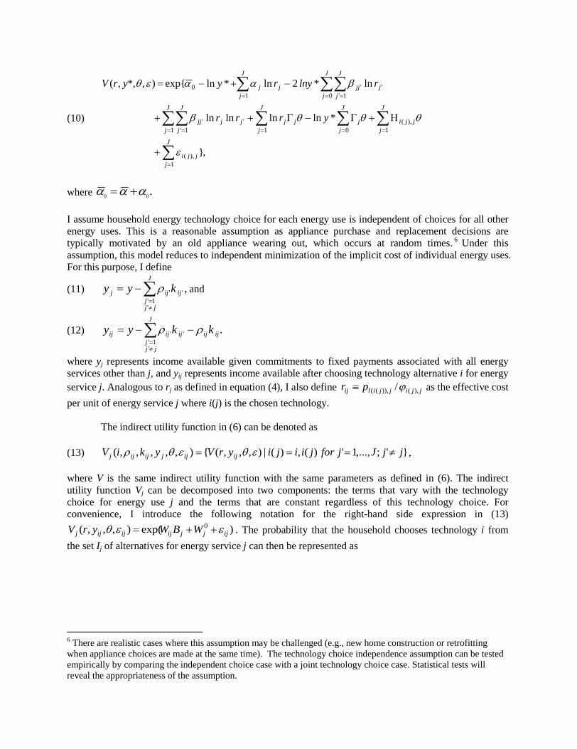
(10)
,}
*lnlnlnln
ln*2ln*lnexp{),*,,(
1),(
1),(
011 1'''
0 1'''
10
J
jjji
J
jjji
J
jj
J
jjj
J
j
J
jjjjj
J
j
J
jjjj
J
jjj
yrrr
rylnryyrV
where .00
I assume household energy technology choice for each energy use is independent of choices for all otherenergy uses. This is a reasonable assumption as appliance purchase and replacement decisions aretypically motivated by an old appliance wearing out, which occurs at random times. 6 Under thisassumption, this model reduces to independent minimization of the implicit cost of individual energy uses.For this purpose, I define
(11) ,
'1'
''
J
jjj
ijijj kyy and
(12) .
'1'
'' ijij
J
jjj
ijijij kkyy
where yj represents income available given commitments to fixed payments associated with all energyservices other than j, and yij represents income available after choosing technology alternative i for energyservice j. Analogous to rj as defined in equation (4), I also define jjijjilij pr ),()),(( / as the effective cost
per unit of energy service j where i(j) is the chosen technology.
The indirect utility function in (6) can be denoted as
(13) }';,...,1')(,)(|),,,({),,,,,( jjJjforjiijiyrVykiV ijijjijijj ,
where V is the same indirect utility function with the same parameters as defined in (6). The indirectutility function Vj can be decomposed into two components: the terms that vary with the technologychoice for energy use j and the terms that are constant regardless of this technology choice. Forconvenience, I introduce the following notation for the right-hand side expression in (13)
)exp(),,,( 0ijjjijijijj WBWyrV . The probability that the household chooses technology i from
the set Ij of alternatives for energy service j can then be represented as
6 There are realistic cases where this assumption may be challenged (e.g., new home construction or retrofittingwhen appliance choices are made at the same time). The technology choice independence assumption can be testedempirically by comparing the independent choice case with a joint technology choice case. Statistical tests willreveal the appropriateness of the assumption.
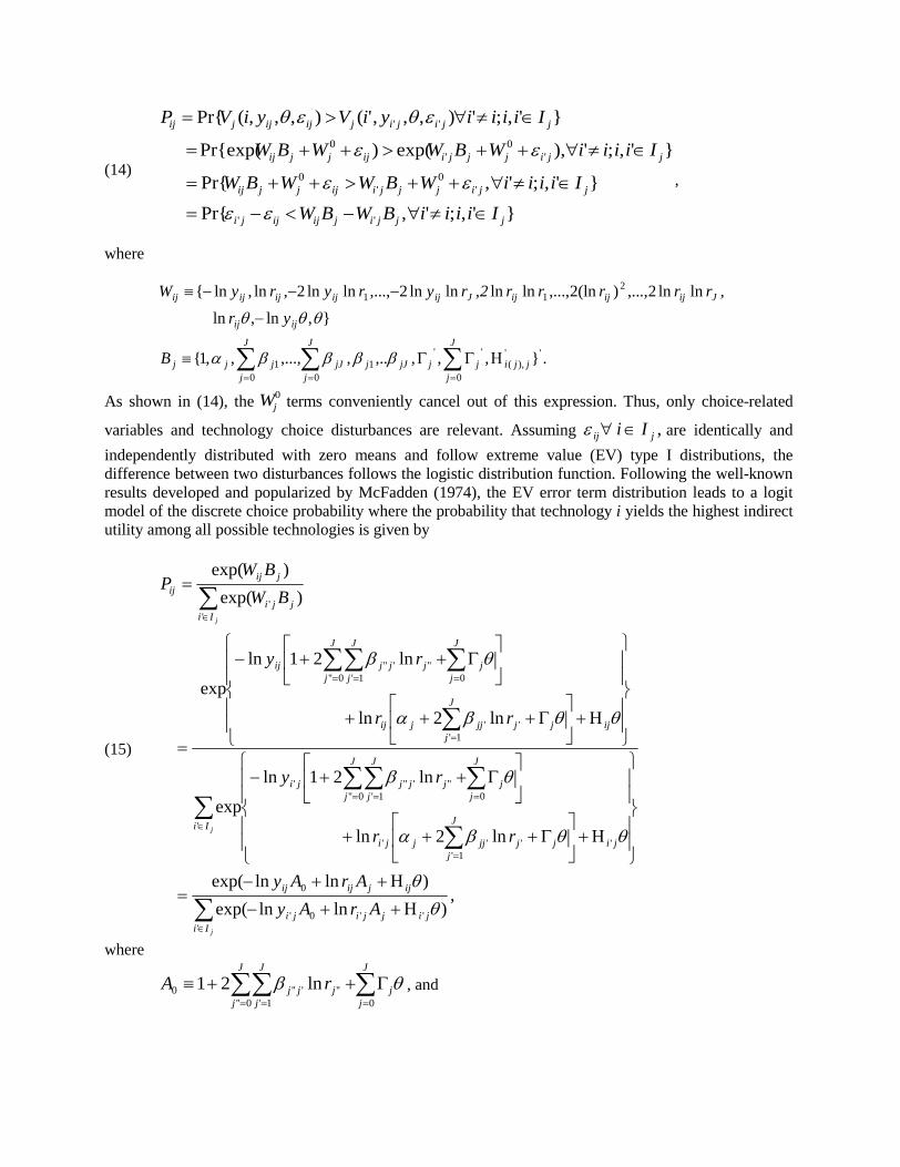
(14)
}',;',Pr{
}',;',Pr{
}',;'),exp()Pr{exp(
}',;'),,,'(),,,(Pr{
''
'0
'0
'0
'0
''
jjjijijijji
jjijjjiijjjij
jjijjjiijjjij
jjijijijijjij
IiiiiBWBW
IiiiiWBWWBW
IiiiiWBWWBW
IiiiiyiVyiVP
,
where
.},,,,..,,...,,,1{
},ln,ln
,lnln2,...,)(ln2,...,lnln,lnln2,...,lnln2,ln,ln{
''),(
0
''1
001
211
jji
J
jjjjJj
J
jjJ
J
jjjj
ijij
JijijijJijijijijij
B
yr
rrrrr2ryryryW
As shown in (14), the 0jW terms conveniently cancel out of this expression. Thus, only choice-related
variables and technology choice disturbances are relevant. Assuming ,jij Ii are identically and
independently distributed with zero means and follow extreme value (EV) type I distributions, thedifference between two disturbances follows the logistic distribution function. Following the well-knownresults developed and popularized by McFadden (1974), the EV error term distribution leads to a logitmodel of the discrete choice probability where the probability that technology i yields the highest indirectutility among all possible technologies is given by
(15)
,)lnlnexp(
)lnlnexp(
ln2ln
ln21ln
exp
ln2ln
ln21ln
exp
)exp(
)exp(
'''0'
0
'
'1'
'''
00'' 1'''''''
1'''
00'' 1''''''
''
j
j
j
Iijijjiji
ijjijij
Ii
jij
J
jjjjjji
J
jj
J
j
J
jjjjji
ijj
J
jjjjjij
J
jj
J
j
J
jjjjij
Iijji
jijij
ArAy
ArAy
rr
ry
rr
ry
BW
BWP
where
J
jj
J
j
J
jjjj rA
00'' 1''''''0 ln21 , and

.ln21'
'' j
J
jjjjjj rA
Thus, A0 and Aj are, in effect, scalars that do not vary with the chosen technology for a given energyservice (and household). Equation (15) shows that when the long-run technology choice decisions and theshort-run energy demands are both derived from the same underlying indirect utility function, coefficientsfor the income variable (lnyij) and price variables (lnrij) in the long-run technology choice model are thesame as those that appear in the short-run fuel demand model in equation (7). In addition, equation (15)shows how the household variables in θ can influence the propensity that the household choosestechnology i for energy use j in a mixed logit framework.
4. Data DescriptionThe empirical study uses micro-data collected for the 2003 Statewide Residential Appliance SaturationStudy (RASS) in California. The study was conducted by the California Energy Commission (CEC) withsponsorship from the major investor-owned utilities in the state. This analysis uses a subsample of 2,408households served by PG&E for both natural gas and electricity in the RASS. The subsample onlyincludes households with both electricity and natural gas consumption in order to empirically estimate thesystem of equations that represents tradeoffs of fuel use both in the short run and the long run as well asbetween short-run and long-run decisions.
The RASS dataset contains variables including household socio-economic characteristics (e.g., income,household size and education level), housing characteristics (e.g., housing type, square-footage, vintageand ownership), appliance holdings by energy use (e.g., technology, age and fuel type), and annualconsumption of electricity and natural gas. The dataset also assigns individual households with climatezone and heating degree days (HDDs) and cooling degree days (CDDs) data, which can help determinehouseholds’ heating and cooling loads. Historic heating and cooling degree days between 1950 and 2003were merged with the RASS based on climate zone.
The PG&E sample presents sufficient variations in household characteristics, fuel consumption andappliance choices for meaningful analysis. Table 1 provides the summary statistics of selected keyvariables of the PG&E sample.
Table 1. Summary statistics of selected variables used in analysis
Variable Mean StandardDeviation Minimum Maximum
Annual electricity use (kWh) 7023.14 3844.53 299.95 33739.49
Annual natural gas (therms) 564.24 278.62 9.02 3058.37
Average income (2000$) 87326.29 47866.74 15000 214454.7
Household size (persons) 2.79 1.46 1 13
Own dwelling dummy 0.92 0.27 0 1
House age (years) 13.73 11.97 1 37
Square footage (sqft) 1890.78 761.82 375 6000
Heating degree days 2630.76 394.53 2207 5267
Cooling degree days 751.07 627.19 0 2060Source: Author’s estimates based on the 2,408 households in the subsample used for estimation.

The analysis of short-run fuel demand and long-run technology choices explicitly models four categoriesof energy services: clothes washing, water heating, space heating, and clothes drying. Together, these fourenergy use categories represent 65 percent of the average household energy consumption.7 These energyuses are chosen for analysis mainly because of the availability and quality of technology data fortechnology choice analysis. In the short-run demand analysis, all other energy uses are grouped in an“other” category.
Despite its rich information, the RASS dataset lacks a few key variables required for the analysis,including fuel prices ( lp ), appliance capital costs ( ijk ), energy efficiency characteristics ( ij ), and
household fixed payments to derive the expenditure variable ( *y ). Historic electricity and natural gastariffs were collected from PG&E and assigned to households based on definitions of service categories.Annual fuel expenditures are estimated using household annual fuel consumption and assigned energyprices. Energy efficiency measures of various appliances are derived from a number of household andmarket survey studies that estimated average energy efficiency levels of existing appliance stock inCalifornia (e.g., RLW Analytics 2001 and 2005, Hanford et al. 1994, and Wenzel et al. 1997). Appliancecosts and energy efficiency characteristics are compiled through the databases developed by the CEC andCPUC and the Lawrence Berkeley Lab. Household fixed payments are estimated based on a regressionanalysis of the relationship between household income and fixed payments using the ConsumerExpenditure Survey.
5. Estimation StrategyThe discrete/continuous model developed in Section 3 consists of a system of simultaneous equationswith continuous demand and discrete choice endogenous variables and a set of exogenous explanatoryvariables consisting of prices, income and household characteristics. This system notably has a recursivestructure between the discrete and continuous components whereby energy consumption depends onobserved appliance choice but not vice versa. I adopt a two-step limited information maximum likelihood(LIML) approach to estimate the model. Because the vast majority of observations on appliance choicepertain to decisions made in a different time period, the assumption of uncorrelated disturbances is wellmotivated. This yields a block recursive system of equations in which blocks of equations can normallybe estimated separately with asymptotic efficiency.
The estimation procedure is implemented as follows. The first step estimates the system of short-rundemand equations (7) and (8) using the iterated feasible generalized nonlinear least squares (FGNLS)method to produce asymptotically consistent estimators. With normally distributed disturbances,estimates using iterated FGNLS are theoretically equivalent to ML estimates (Greene 2008). The adding-up condition implies that covariance matrix is singular and nondiagonal. Therefore, one equation isdropped from the system to obtain identification.8
Then, the technology choice equations are evaluated separately using the method of ML without imposingany structural constraints. Because choices of different appliances are made at different points in time,correlation among the disturbances is likely minor if present at all, in which case separate estimation doesnot sacrifice efficiency aside from ignoring parameter constraints among equations. Four separate energytechnology choice equations are then estimated, representing clothes washing (cw), water heating (wh),space heating (sph) and clothes drying (cd). Technology choice sets consist of two choice alternatives for
7 An initial analysis was carried out which consider joint choices of water heater and space heater given the possiblecorrelation of fuel choices for these two energy services. However, a statistical test of the nested model of fuelchoices cannot reject the null hypothesis that fuel choices for water heating and space heating are independent.8 Specification tests show that among different combinations using two of the three budget share equationspecifications, the system of budget share equations for the numeraire and natural gas yields the highest loglikelihood value, although all choices should yield the same asymptotic results.

clothes washing and clothes drying. Thus a binary logit choice model is appropriate. For water heatingand space heating, three choice alternatives are involved in each case so a multinomial logit choice modelis appropriate.
In the second step, equation (15) is re-estimated by imposing parametric constraints on parameters A0 andAj implied by parameter estimates from the short-run demand model estimated using the maximumlikelihood obtained in step one. The vector of the remaining parameters is estimated, producing the MLestimator of the parameters and the associated ML estimator of the covariance matrix of the parameters.Then, the covariance matrix is corrected that accounts for the covariance matrix estimator of the short-runparameters to obtain the asymptotic covariance matrix. The correction follows the procedure developedby Murphy and Topel (2002).
6. Estimation ResultsThe results of the short-run demand analysis and the technology choice analysis are summarized inSection 6.1 and 6.2, respectively.
6.1 Short-Run Energy DemandTable 1 below presents the estimation results of four specifications using the FGNLS procedure. Model
1a includes only price variables jrln , the income variable *ln y , and demand interaction terms. Model 1b
builds on Model 1a and adds household-demand interaction terms. Inclusion of household and demandinteraction terms is guided by the features of energy service demands and significance of statistical tests.A log likelihood ratio test between Model 1a and Model 1b rejects the null hypothesis that the household-demand interaction terms in the model are jointly zero with a p-value less than 0.001, suggestinghousehold variables—household size, dwelling square footage, heating degree days and the age ofdwelling in this specification—influence household energy demand significantly.
Model 1c builds on Model 1b and instead of using average energy efficiency indicators to derive the pricevariable for clothes washing, cwrln , it treats energy efficiency of clothes washers as an estimable linearfunction of the energy efficiency standards (“Standard”) and the EnergyStar information program(“EnergyStar”) aside from an error term, i.e., )()()()( lnln)/ln(ln cwicwlcwicwlcw ppr , where
.0)(,ln )()(21)( cwicwiicwi eEeEnergyStarStandard Average energy efficiency indicators are
used to derive the price variables for water heating, space heating, and clothes drying. Compared withModel 1b, the model fit of Model 1c improves significantly with much higher log likelihood and pseudo-R2 values with a p-value less than 0.001. The results indicate potential measurement errors by using theaverage energy efficiency of the clothes washer stock in the demand analysis. This is likely due to asubstantial improvement in energy efficiency performance of clothes washers over the past two decadesas a result of technology improvement and energy efficiency policy.
Changes in the energy efficiency performance of water heaters, space heaters and clothes dryers weremodest during the study period. Nonetheless, a specification test is performed to see whether use ofaverage energy efficiency indicators for water heaters is statistically equivalent to modeling energyefficiency of water heaters as an estimable function of appliance age (Model 1d). In Model 1d, the energyefficiency of water heaters is modeled as a linear function of the age of water heater (“age_wh”) and anerror term, i.e., .0)(,ln )()(1)( whiwhiiwhi eEeage_wh The log likelihood ratio test between Model 1d

Table 1. Coefficient estimates of the short-run demand equations
Coefficient Definition
Model 1a Model 1b Model 1c Model 1d
Without
household
variables
With
householdvariables
With energyefficiency of
clotheswashers
With energyefficiencies of
clotheswashers andwater heaters
a0 intercept –numeraire
1.07892*** 0.92969*** 0.81503*** 0.80212***
(149.241) (166.703) (84.181) (65.717)
a1 intercept-cw -0.03500* -0.03577*** 0.06756*** 0.10859***
(-2.385) (-4.121) (5.456) (6.854)
a2 intercept-wh 0.06316 0.02998 -0.02994 -0.01002
(1.279) (0.893) (-0.857) (-0.226)
a3 intercept-cd -0.03620** 0.03689*** 0.03209*** -0.00099
(-3.101) (4.138) (3.774) (-0.118)
a4 intercept-sph -0.03062 0.02915 -0.02322 -0.01592
(-0.882) (1.214) (-0.925) (-0.619)
01 cross demandnumeraire-cw
-0.01047*** 0.01596*** 0.01142*** 0.01094***
(-8.144) (14.497) (7.430) (6.680)
02 cross demandnumeraire-wh
0.00265* 0.00341* -0.00265 -0.00222
(2.447) (2.498) (-1.401) (-1.226)
03 cross demand
numeraire-cd
0.00158* 0.00194*** 0.00116 -0.00180**
(2.425) (3.736) (1.764) (-3.114)
(Continued on next page)

04 cross demand
numeraire-sph
-0.00072 0.00643*** 0.00271 0.00318*
(-0.667) (4.798) (1.731) (2.022)
05 cross demand
numeraire-oth
0.04241*** 0.02293*** 0.03754*** 0.03999***
(32.445) (12.234) (14.173) (14.105)
11 own demand
cw
0.02324*** 0.02383*** 0.04820*** 0.05129***
(7.540) (30.328) (15.794) (15.795)
12 cross demand
cw-wh
-0.00609*** 0.00056*** -0.00208 -0.0023
(-6.231) (3.471) (-1.127) (-1.156)
13 cross demand
cw-cd
0.00042 0.00046** -0.00252** -0.00085
(1.395) (2.749) (-2.769) (-0.719)
22 own demand
wh
0.09579 0.01308 -0.01877 0.00505
(1.630) (0.352) (-0.437) (0.147)
25 cross demand
wh-oth
-0.09331 -0.01231 0.01938 -0.00501
(-1.582) (-0.331) (0.450) (-0.147)
33 own demand
cd
-0.00422** 0.00260*** 0.00403*** -0.00057
(-3.250) (3.454) (3.912) (-0.344)
44 own demand
sph
-0.11814 -0.02305 -0.0569 -0.06193
(-1.877) (-0.579) (-1.445) (-1.559)
45 cross demand
sph-oth
0.12151 0.02735 0.05789 0.0642
(1.921) (0.685) (1.468) (1.615)

55 own demand
oth
-0.06206 -0.0249 -0.07699 -0.05884
(-0.783) (-0.496) (-1.455) (-1.200)
d1 hh_size-wh
interaction
-0.00038*** -0.00037*** -0.00038***
(-7.049) (-6.649) (-6.620)
d2 sqft–sph
interaction
0.00053*** 0.00069*** 0.00072***
(4.781) (6.031) (6.080)
d3 age–oth
interaction
-0.00069*** -0.00074*** -0.00075***
(-10.822) (-11.098) (-10.888)
d4 hhd–sph
interaction
0.00213*** 0.00220*** 0.00226***
(10.792) (10.869) (10.776)
1 Standard-cw -0.00515 -0.00521
(-0.428) (-0.430)
2 EnergyStar-cw -0.00647 -0.00714
(-0.640) (-0.694)
1 technology 0.04578
change-wh (0.146)
Observations 2408 2408 2408 2408
Log likelihood 14827 15414 15516 15519
R2 numeraire 0.385 0.579 0.604 0.604
R2 gas 0.414 0.777 0.788 0.788
Notes: (1) Asterisks in the table denote significance in terms of p-values as follows: ‘*’ for p < 0.05, ‘**’ for p <0.01, and ‘***’ for p < 0.001. (2) Values in parentheses are t-statistics.

and Model 1c suggests that modeling energy efficiency of water heaters as a function of technologychange is preferred to using average energy efficiency indicators with a p-value of 0.021.9 Model 1d isthus used as the main specification for subsequent discussions and the parametric estimates imposed inthe second stage estimation of technology choices.
The coefficients derived from the estimation are difficult to interpret on their own. Demand elasticities aremore revealing. The estimated income and own price elasticities are presented in Table 2 and 3 below,respectively. Cross price elasticities between electricity and natural gas are unlikely to be important assubstitution between the fuels is limited in the short run.
Table 2. Estimated short-run income elasticities of demand for fuels
Model Mean StandardDeviation Minimum Maximum
Electricity
Model 1a 0.0816 0.0843 -0.2623 2.1148
Model 1b 0.3436 0.0804 0.2560 0.8703
Model 1c 0.5032 0.0658 0.4267 1.0038
Model 1d 0.4182 0.1786 0.3189 1.6974
Natural Gas
Model 1a -0.0698 0.0358 -0.0933 0.1417
Model 1b -0.7127 0.2457 -0.9537 0.8085
Model 1c -0.3096 0.1201 -0.4029 0.4024
Model 1d -0.4201 0.1639 -0.5963 0.5113
Table 3. Estimated short-run price elasticities of demand for fuels
Model Mean StandardDeviation Minimum Maximum
Electricity
Model 1a 0.2533 0.1480 0.1538 2.8310
Model 1b -0.1313 0.0609 -0.5339 -0.0474
Model 1c -0.0641 0.0831 -0.7499 -0.0359
Model 1d -0.1343 0.1410 -1.0913 -0.0677
9 An additional specification test shows that using average energy efficiency indicators for space heating systems isnot statistically different from explicitly modeling the energy efficiency of space heating systems with a p-value of0.072. Thus, using average space heating energy efficiency indicators does not introduce significant measurementerrors.

Natural Gas
Model 1a -0.2060 0.4769 -0.3311 2.8901
Model 1b -0.1473 0.1992 -0.2611 1.0758
Model 1c -0.1262 0.1107 -0.3432 0.6230
Model 1d -0.1188 0.1439 -0.1775 0.8373
The mean estimates of income elasticity for electricity are positive in all four specifications and less thanunity (Table 2). Model 1d, the preferred specification, has a mean estimated income elasticity of 0.418 forelectricity and a range between 0.319 and 1.697. The maximum estimates of income elasticity forelectricity are greater than unity in three out of the four cases. As expected, the results show thatelectricity is a superior good. The estimated mean income elasticity for natural gas is consistentlynegative in all four cases. However, in all four cases, income elasticities range widely over both negativeand positive values. For Model 1d, the mean estimate of income elasticity for natural gas is -0.420 with aminimum value of -0.596 and a maximum value of 0.511. These results suggest that natural gas is aninferior good for many households, which is not surprising.
The mean estimates of own price elasticity for electricity are all negative except for Model 1a (Table 3),the least preferred model. For Model 1d, the estimated own price elasticity for electricity has a mean of -0.134 and a range between -1.091 and -0.068, which appears quite plausible. The mean estimates of priceelasticity for natural gas are consistently negative. Similar to estimates of income elasticity for natural gas,however, the ranges of estimates among individual households include both negative and positive values.In Model 1d, the estimate of own price elasticity for natural gas has a mean of -0.119 and a range between-0.177 and 0.837, although very few households (3.3 percent) fall in the positive range.
6.2 Energy Technology Choices
Clothes Washer ChoicesTable 4 reports the estimation results of the binary logit model of clothes washer choices with fourspecifications. Model cw1a and Model cw1b investigate two specifications using average energyefficiency indicators to derive the expected operating costs; Model cw2a and Model cw2b have the samesets of specifications except that the perceived energy efficiency of the choice alternatives is modeled as afunction of the energy efficiency standards and the Energy Star program as in the short-run demandanalysis. Model 1a and Model 2a evaluate the roles of the initial capital cost and the expected operatingcost of technology alternatives in clothes washer choices. Variable ln_incCW is the negative of thelogarithm of household income not already committed to fixed payments minus the annualized capitalcosts between the choice alternatives. In Model cw1a, the expected operating cost is represented by thelogarithm of the operating cost derived from average energy efficiency indicators (ln_oCostCW). InModel cw2a, the expected operating cost consists of three components: the logarithm of fuel price(ln_fuel), a dummy variable representing the presence of clothes washer energy efficiency standards(Standard), and a dummy variable representing the presence of clothes washer Energy Star criteria(EnergyStar).
Model cw1b and Model cw2b add household variables to examine whether household characteristics mayhave influenced clothes washer choices. Specifically, three household variables are included: (1) thehome ownership dummy (own), (2) the household size (household size), and (3) a college educationdummy (college). The college education dummy is an instrument to represent consumers’ ability tounderstand and interpret energy consumption and performance information pertaining to home appliances.

A second step of constrained estimator is performed with the specification of Model cw2b by imposingparametric constraints on the common variables (ln_incCW and ln_fuel) based on coefficient estimatesfrom the short-run demand model (Model 1d). Column 5 in Table 4 presents the results of the constrainedestimation as Model cw2b*.
Table 4. Estimated coefficients of the clothes washer choice model
RegressorModel
cw1a cw1b cw2a cw2b cw2b*
ln_incCW -100.190*** -65.476*** -184.026*** -145.925***
(-5.47) (-3.95) (-4.50) (-3.62)
ln_oCostCW 1.516*** 2.738***
(20.96) (8.60)
ln_fuel 0.635 0.695
(0.73) (0.78)
Standard 1.127** 1.092** 0.889*
(2.70) (2.61) (2.12)
EnergyStar 2.144*** 2.136*** 1.925***
(7.68) (7.66) (8.37)
Own 0.620 0.635 0.847*
(1.94) (1.92) (2.59)
Household size 0.102* 0.049 0.062
(2.56) (0.99) (1.39)
College 0.586*** 0.447* 0.798***
(3.71) (2.73) (5.00)
Constant -2.683 -3.689* -5.910***
(-1.60) (-2.09) (-11.15)
Observations 2408 2408 2408 2408 2408
Log likelihood -841 -828 -718 -712 -734
Notes: (1) Asterisks in the table denote significance in terms of p-values as follows: ‘*’ for p < 0.05, ‘**’ for p <0.01, and ‘***’ for p < 0.001. (2) Values in parentheses are t-statistics. (3) A top-loading clothes washer is the basecase in this analysis.

As shown in Table 4, the coefficient of the household expenditure variable that incorporates the initialcost of clothes washer alternatives (ln_incCW) is significant across all specifications. The negativecoefficient of ln_incCW suggests that a reduction in the initial capital cost will increase the probability offront-loading clothes washer adoption. The expected operating cost, derived using average energyefficiency indicators (Model cw1a and Model cw1b), also significantly influences clothes washer choices.
The positive coefficient of ln_oCostCW implies that an increase in expected operating cost encouragesadoption of front-loading clothes washers. When the perceived energy efficiency of choice alternatives ismodeled as a function of policy interventions (Model cw2a and Model cw2b), the positive coefficient ofln_fuel also implies that a higher energy price increases the propensity of front-loading clothes washerchoice. However, the effect of energy price appears not to be statistically significant. This could suggestan exceptionally high discount rate or great uncertainty regarding future energy prices on the part ofconsumers when they make their choices.
When the household perception of energy efficiency of alternative clothes washer choices is modeled as afunction of the energy efficiency standard and the Energy Star program (Model cw2 in columns 3 and 4),the model fit improves significantly compared to using average energy efficiency indicators, suggestingthat households’ formation of energy efficiency perceptions for clothes washers is more likely influencedby information conveyed through energy efficiency standards and Energy Star labels. The positive andsignificant coefficients for both the energy efficiency standards and Energy Star program suggest thatthese policy interventions have strong influences over the propensity of front-loading clothes washeradoption.
A log ratio test of the restricted model (Model cw2b*) and the unrestricted model (Model cw2b) rejectsthe null hypothesis that the common parameters between the short-run demand model and the long-runclothes washer choice model are equivalence with a p-value less than 0.001. This is a very differentoutcome from the results for the other three end uses analyzed below. The rejection of parametricequivalence between the short-run demand model and the clothes washer choice model raises concern thatthe household clothes washer choice behavior may be mis-specified in the preference function. InCalifornia where water supply is constrained, the water saving benefits of front-loading washers may be afurther significant factor that drives clothes washer choice decisions. Unfortunately, water price data werenot available to further test this hypothesis at the time this study was completed.
Estimated coefficients are fairly consistent across specifications except for the common parameters.Household characteristics are found to play a role in the choice decisions. Specifically, having a collegeeducation positively and significantly influences the choice of front-loading clothes washers. Homeownership also positively influences the choice of front-loading washers. However, the significance ofthis effect varies by specification. In addition, having a larger household size appears to favor adoption oftop-loading clothes washers, possibly due to preference for the larger capacity of top-loading washersover the more compact front-loading washers. But the effect of household size is not significant exceptfor specification Model cw2b.
Water Heater ChoicesTable 5 reports three specifications of the multinomial logit model of water heater choices. Model wh1aevaluates the effect of a household expenditure term that incorporates the initial capital cost of waterheaters and the effect of expected operating cost of alternative water heaters. Two variables are includedin Model wh1a: the negative of the logarithm of household income not already committed to fixedpayments minus annualized capital costs of water heater choice alternatives (ln_incWH), and thelogarithm of the expected operating costs of technology alternatives using average energy efficiencyindicators (ln_oCostWH). Since the energy efficiency of water heaters has only changed moderately
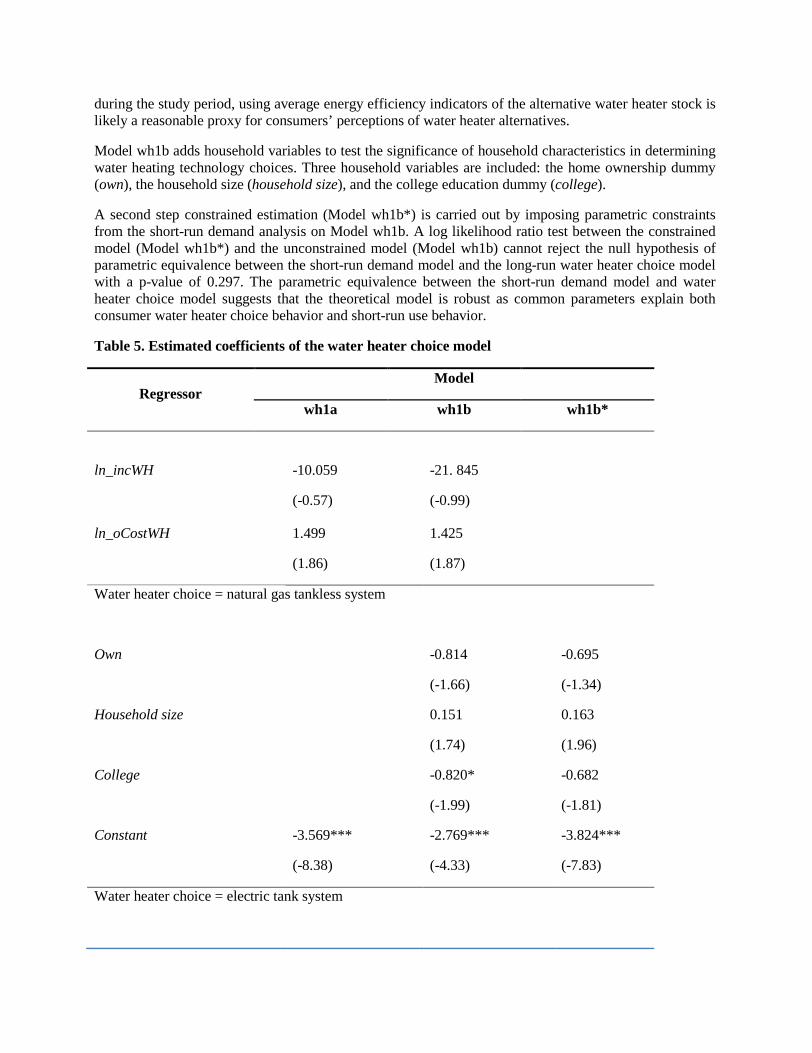
during the study period, using average energy efficiency indicators of the alternative water heater stock islikely a reasonable proxy for consumers’ perceptions of water heater alternatives.
Model wh1b adds household variables to test the significance of household characteristics in determiningwater heating technology choices. Three household variables are included: the home ownership dummy(own), the household size (household size), and the college education dummy (college).
A second step constrained estimation (Model wh1b*) is carried out by imposing parametric constraintsfrom the short-run demand analysis on Model wh1b. A log likelihood ratio test between the constrainedmodel (Model wh1b*) and the unconstrained model (Model wh1b) cannot reject the null hypothesis ofparametric equivalence between the short-run demand model and the long-run water heater choice modelwith a p-value of 0.297. The parametric equivalence between the short-run demand model and waterheater choice model suggests that the theoretical model is robust as common parameters explain bothconsumer water heater choice behavior and short-run use behavior.
Table 5. Estimated coefficients of the water heater choice model
RegressorModel
wh1a wh1b wh1b*
ln_incWH -10.059 -21. 845
(-0.57) (-0.99)
ln_oCostWH 1.499 1.425
(1.86) (1.87)
Water heater choice = natural gas tankless system
Own -0.814 -0.695
(-1.66) (-1.34)
Household size 0.151 0.163
(1.74) (1.96)
College -0.820* -0.682
(-1.99) (-1.81)
Constant -3.569*** -2.769*** -3.824***
(-8.38) (-4.33) (-7.83)
Water heater choice = electric tank system

Own -1.260*** -1.269***
(-4.25) (-4.28)
Household size -0.052 -0.071
(-0.49) (-0.66)
College 0.370 0.428
(1.44) (1.63)
Constant -5.495*** -4. 424*** -2.388***
(-4.85) (-3.99) (-6.20)
Observation 2408 2408 2408
Log_likelihood -496 -483 -485
Notes: (1) Asterisks in the table denote significance in terms of p-values as follows: ‘*’ for p < 0.05, ‘**’ for p <0.01, and ‘***’ for p < 0.001. (2) Values in parentheses are t-statistics. (3) A natural gas tank system is the base casein the analysis.
In contrast to the clothes washer choice analysis, the household expenditure variable (ln_incWH) is not astatistically significant determinant of water heater choices. The expected operating cost (ln_oCostWH) isalso a statistically insignificant predictor of water heater choices.
Home ownership is a significant predictor of water heater choices. A home owner is estimated to be morelikely to choose a gas tank system over an electric tank system compared to a renter. This can beexplained by the fact that a home owner is more likely to pay for the operating cost of water heater usagethan a renter. Along this line of thinking, one would expect that a home owner is more likely to choose atankless system than a tank system, which has much lower operating cost. The regression results showthat a home owner is less likely to choose a tankless gas system over a tank system, but the estimatedcoefficient is statistically insignificant. The logistics as well as high cost of retrofitting an existing homewith a tankless system may be an important deterrent.
The college education dummy is also a significant explanatory variable for water heater choices. Ahousehold with at least a college education is also more likely to choose a natural gas tank water heaterover a tankless system but more likely to choose an electric tank system over a natural gas tank system,although only the former relationship is statistically significant. Larger household sizes tend to choose atankless system over a natural gas tank system and a natural gas tank system over an electric tank system,but neither estimated effect is statistically significant.
Space Heating System ChoicesTable 6 reports the results of three specifications of the multinomial logit model of space heating systemchoices. Similar to water heater choice model, Model sph1a evaluates the logarithm of householdexpenditure, which incorporates the capital costs of choice alternatives (ln_incSPH) and the logarithm ofthe expected operating costs of technology alternatives using average energy efficiency indicators(ln_oCostSPH). Using average energy efficiency estimates is reasonable in this case as the energyefficiency of space heating systems did not change dramatically during the study period. Model sph1bincludes household variables to detect whether housing and household characteristics influence space

heating technology choices. Four household variables are included: (1) the home ownership dummy(own), (2) age of the house (house age), (3) historic mean heating degree days between 1985 and the yearof system installation (hdd_mean), and (4) the college education dummy (college).
A second step constrained estimation (Model sph1b*) is also carried out by imposing parametricconstraints from the short-run demand analysis on Model sph1b.
Table 6. Estimated coefficients of the space heating system choice model
RegressorModel
sph1a sph1b sph1b*
ln_incSPH -3.083 -4.576
(-0.78) (-1.62)
ln_oCostSPH 0.430 0.310
(0.91) (0.65)
Space heater choice = natural gas radiator
Own -1.038 -0.964
(-1.36) (-1.21)
House age -0.258 -0.259
(-0.68) (-0.78)
Hdd_mean 2.881** 2.861*
(2.60) (2.39)
College -0.198 -0.106
(-0.31) (-0.16)
Constant -5.244*** -11.413*** -11.726***
(-13.97) (-3.35) (-3.43)
Space heater choice = electric central forced-air system
Own -0.050 -0.054
(-0.12) (-0.13)
House age 0.285** 0.291**
(3.08) (3.16)
Hdd_mean -0.322 -0.368
(-0.78) (-0.84)
College -0.528* -0.517*
(-2.28) (-2.24)
Constant -3.955*** -3.105* -2.566*
(-6.14) (-2.38) (-2.19)
Observation 2408 2408 2408
log_likelihood -412 -400 -399
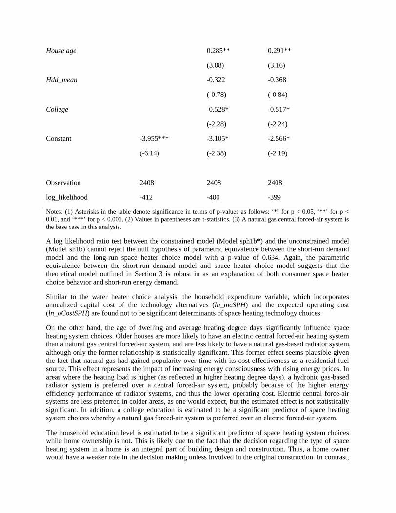
Notes: (1) Asterisks in the table denote significance in terms of p-values as follows: ‘*’ for p < 0.05, ‘**’ for p <0.01, and ‘***’ for p < 0.001. (2) Values in parentheses are t-statistics. (3) A natural gas central forced-air system isthe base case in this analysis.
A log likelihood ratio test between the constrained model (Model sph1b*) and the unconstrained model(Model sh1b) cannot reject the null hypothesis of parametric equivalence between the short-run demandmodel and the long-run space heater choice model with a p-value of 0.634. Again, the parametricequivalence between the short-run demand model and space heater choice model suggests that thetheoretical model outlined in Section 3 is robust in as an explanation of both consumer space heaterchoice behavior and short-run energy demand.
Similar to the water heater choice analysis, the household expenditure variable, which incorporatesannualized capital cost of the technology alternatives (ln_incSPH) and the expected operating cost(ln_oCostSPH) are found not to be significant determinants of space heating technology choices.
On the other hand, the age of dwelling and average heating degree days significantly influence spaceheating system choices. Older houses are more likely to have an electric central forced-air heating systemthan a natural gas central forced-air system, and are less likely to have a natural gas-based radiator system,although only the former relationship is statistically significant. This former effect seems plausible giventhe fact that natural gas had gained popularity over time with its cost-effectiveness as a residential fuelsource. This effect represents the impact of increasing energy consciousness with rising energy prices. Inareas where the heating load is higher (as reflected in higher heating degree days), a hydronic gas-basedradiator system is preferred over a central forced-air system, probably because of the higher energyefficiency performance of radiator systems, and thus the lower operating cost. Electric central force-airsystems are less preferred in colder areas, as one would expect, but the estimated effect is not statisticallysignificant. In addition, a college education is estimated to be a significant predictor of space heatingsystem choices whereby a natural gas forced-air system is preferred over an electric forced-air system.
The household education level is estimated to be a significant predictor of space heating system choiceswhile home ownership is not. This is likely due to the fact that the decision regarding the type of spaceheating system in a home is an integral part of building design and construction. Thus, a home ownerwould have a weaker role in the decision making unless involved in the original construction. In contrast,
the two types of housing that dominate the PG&E area of California are the older homes that are beyondtheir first owner and the more recent large-scale developments of builders. Thus, energy technologydurables such as space heating and water heating equipment are likely heavily determined by developersif not the more aged housing stock.
While one might argue that a developer would tailor these choices to potential buyers’ preferences, ahome buyer likely will weigh other attributes of a house (such as location and size) more heavily than thetype of space heating system. The significance of college education in choosing a natural gas spaceheating system over an electricity-based space heating system, on the other hand, suggests that ahousehold with better ability to interpret energy performance information of different energy systems ismore likely to make a rational choice of the system that has lower operating cost.
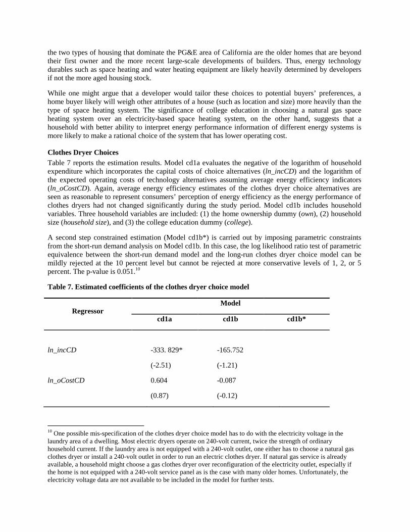
Clothes Dryer ChoicesTable 7 reports the estimation results. Model cd1a evaluates the negative of the logarithm of householdexpenditure which incorporates the capital costs of choice alternatives (ln_incCD) and the logarithm ofthe expected operating costs of technology alternatives assuming average energy efficiency indicators(ln_oCostCD). Again, average energy efficiency estimates of the clothes dryer choice alternatives areseen as reasonable to represent consumers’ perception of energy efficiency as the energy performance ofclothes dryers had not changed significantly during the study period. Model cd1b includes householdvariables. Three household variables are included: (1) the home ownership dummy (own), (2) householdsize (household size), and (3) the college education dummy (college).
A second step constrained estimation (Model cd1b*) is carried out by imposing parametric constraintsfrom the short-run demand analysis on Model cd1b. In this case, the log likelihood ratio test of parametricequivalence between the short-run demand model and the long-run clothes dryer choice model can bemildly rejected at the 10 percent level but cannot be rejected at more conservative levels of 1, 2, or 5percent. The p-value is 0.051.10
Table 7. Estimated coefficients of the clothes dryer choice model
RegressorModel
cd1a cd1b cd1b*
ln_incCD -333. 829* -165.752
(-2.51) (-1.21)
ln_oCostCD 0.604 -0.087
(0.87) (-0.12)
10 One possible mis-specification of the clothes dryer choice model has to do with the electricity voltage in thelaundry area of a dwelling. Most electric dryers operate on 240-volt current, twice the strength of ordinaryhousehold current. If the laundry area is not equipped with a 240-volt outlet, one either has to choose a natural gasclothes dryer or install a 240-volt outlet in order to run an electric clothes dryer. If natural gas service is alreadyavailable, a household might choose a gas clothes dryer over reconfiguration of the electricity outlet, especially ifthe home is not equipped with a 240-volt service panel as is the case with many older homes. Unfortunately, theelectricity voltage data are not available to be included in the model for further tests.
Own -0.430** -0.471**
(-2.65) (-2.92)
Household size -0.106*** -0.111***
(-3.51) (-3.98)
College -0.029 -0.080
(-0.32) (-0.92)
Constant -0.636 1.138 1.155
(-0.61) (1.01) (6.34)
Observations 2408 2408 2408
Log likelihood -1624 -1615 -1618
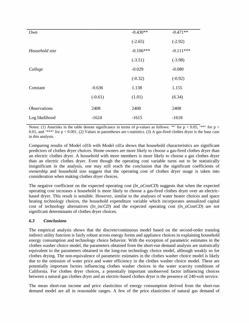
Notes: (1) Asterisks in the table denote significance in terms of p-values as follows: ‘*’ for p < 0.05, ‘**’ for p <0.01, and ‘***’ for p < 0.001. (2) Values in parentheses are t-statistics. (3) A gas-fired clothes dryer is the base casein this analysis.
Comparing results of Model cd1b with Model cd1a shows that household characteristics are significantpredictors of clothes dryer choices. Home owners are more likely to choose a gas-fired clothes dryer thanan electric clothes dryer. A household with more members is more likely to choose a gas clothes dryerthan an electric clothes dryer. Even though the operating cost variable turns out to be statisticallyinsignificant in the analysis, one may still reach the conclusion that the significant coefficients ofownership and household size suggest that the operating cost of clothes dryer usage is taken intoconsideration when making clothes dryer choices.
The negative coefficient on the expected operating cost (ln_oCostCD) suggests that when the expectedoperating cost increases a household is more likely to choose a gas-fired clothes dryer over an electric-based dryer. This result is sensible. However, similar to the analyses of water heater choices and spaceheating technology choices, the household expenditure variable which incorporates annualized capitalcost of technology alternatives (ln_incCD) and the expected operating cost (ln_oCostCD) are notsignificant determinants of clothes dryer choices.
6.3 Conclusions
The empirical analysis shows that the discrete/continuous model based on the second-order translogindirect utility function is fairly robust across energy forms and appliance choices in explaining householdenergy consumption and technology choice behavior. With the exception of parametric estimates in theclothes washer choice model, the parameters obtained from the short-run demand analysis are statisticallyequivalent to the parameters obtained in the long-run technology choice model, although weakly so forclothes drying. The non-equivalence of parametric estimates in the clothes washer choice model is likelydue to the omission of water price and water efficiency in the clothes washer choice model. These arepotentially important factors influencing clothes washer choices in the water scarcity conditions ofCalifornia. For clothes dryer choices, a potentially important unobserved factor influencing choicesbetween a natural gas clothes dryer and an electric-based clothes dryer is the presence of 240-volt service.
The mean short-run income and price elasticities of energy consumption derived from the short-rundemand model are all in reasonable ranges. A few of the price elasticities of natural gas demand of

individual households are implausible ranges but no more than typically obtained with the flexibility ofthe translog model.
7. Policy Implications for Household Energy Efficiency
Residential consumer energy consumption is a critical aspect of energy and climate changepolicy. Findings from the empirical analysis using the unified modeling framework haveimportant implications for policy design aimed to reduce greenhouse gas emissions and improveenergy efficiency in the residential sector.
7.1 Energy-efficient Technology Adoption
This study confirms two important market failures with respect to household energy technology choicebehavior: the principal/agent problem and information imperfection. Home ownership appears tosignificantly influence household choices of some energy durables, suggesting that policy programstargeting residential energy efficiency should carefully distinguish the principal decision makers andappropriately differentiate market segments.
In the case of clothes washer choices, the voluntary, information-based Energy Star program emerges asthe most significant factor influencing adoption of energy-efficient front-loading clothes washers,followed by energy efficiency standards. The establishment of Energy Star criteria for clothes washersproduces an average increase in the propensity of energy-efficient front-loading clothes washers by 17percent. The presence of energy efficiency standards is predicted on average to increase the propensity offront-loading washers adoption by 8 percent. The results suggest that policy programs aimed at providingenergy technology performance information are highly effective in promoting the adoption of energy-efficient technology at the household level as these programs likely reduce consumers’ search cost. In fact,they may override cost considerations that are highly uncertain at the point of decision making in the store.
Surprisingly, the financial incentives for energy-efficient appliances, such as through popular federalincome tax credits or federal and state rebate programs, are found to be far less effective in influencingthe adoption of energy-efficient appliances. For instance, a $100 reduction in the purchase cost of energy-efficient front-loading washers increases the propensity of front-loading clothes washer adoption by only0.5 percent. Perhaps consumers who take advantage of such programs have a priori preferences forenergy efficiency, so that financial incentives only provide a windfall to such consumers. In the case ofwater heater and space heating system choices, the capital cost of technology alternatives appear to be aninsignificant determinant of technology choices, suggesting that changes in the relative cost of energy-efficient technologies would have limited impacts on their adoption.11 Given their popularity, thesefinancial incentive programs and their cost-effectiveness should be carefully examined.
Furthermore, contrary to the claim that incentives for the adoption of new technologies is greater undermarket-based instruments than under direct regulation (e.g., by Jaffe et al. 2003), this empirical studyfinds that market-based policy instruments, such as a carbon cap-and-trade program or carbon taxeswhich induce energy price changes, have limited impacts on energy-efficient technology adoptiondecisions at the household level. For instance, a 20 percent increase in energy (electricity) price increasesthe propensity of front-loading washer adoption by only 2.5 percent.
11 However, it should be pointed out that the technology choice analyses for water heating and space heatingexamine the choices among broad categories of technology systems (e.g., a tank water heater versus a tanklesssystem), rather than choices among different brands and models of a technology that have varying energy efficiencyperformance. Further, the absence of statistical significance of cost variables in these cases may be largely due to theminor differences in costs among technologies even though consumers may respond to more substantial costvariation. Inference about incentive policy based on these results should be made carefully.

7.2 Short-run Household Energy EfficiencyThe study finds that in the short-run, energy price-induced household energy efficiency is moderate.According to the analysis, the average price elasticity is -0.13 for electricity and -0.12 for natural gas.Therefore, a 20 percent increase in the electricity price on average would reduce its consumption by 2.6percent; a 20 percent increase in the natural gas price on average would reduce its consumption by 2.4percent. These results are reasonable given estimates and conventional wisdom that implies householdenergy demand is highly inelastic in the short run.
The short-run demand analysis also highlights the importance of using accurate estimates of applianceenergy efficiency in energy demand modeling. The energy efficiency level of household energy durablesaffects the amount of energy consumed by a household to meet energy service demands. Very often, theenergy efficiency of home appliances is unknown. At best, modelers and researchers rely on marketsurveys with estimates of the average energy efficiency of the appliance stock. In this study, twoalternative representations of appliance energy efficiency are tested for clothes washers and water heaters.The first approach uses average energy efficiency indicators of energy technology based on marketsurveys. The second approach assumes household appliance energy efficiency is unobserved andexplicitly models energy efficiency as a function of technological change and possible policyinterventions such as energy efficiency standards. Compared to the survey data on average energyefficiency, embedding this causal model of energy efficiency improves model fit for clothes washers andwater heaters significantly, producing higher log likelihood values, and suggesting potential measurementerrors by using average energy efficiency data on the appliance stock.
ReferencesAigner, D.J., C. Sorooshian, and P. Kerwin. 1984. “Conditional demand analysis for estimatingresidential end-use load profiles.” Energy Journal 5(3), 81-97.
Anderson, S.T., and R.G. Newell. 2002. Information Programs for Technology Adoption: The Case ofEnergy-Efficiency Audits, Resources for the Future RFF Discussion Paper 02-58. Washington DC.
Archibald, R.B., D.H. Finifter and C.E. Moody Jr. 1982. “Seasonal variation in residential electricitydemand: evidence from survey data.” Applied Economics 14, 167-181.
Baker, P., R. Blundell, J. Michlewright. 1989. “Modelling Household Energy Expenditures Using Micro-Data,” The Economic Journal 99(397): 720-738
Balestra, P., and M. Nerlove. 1966. “Pooling gross section and time series data in the estimation of adynamic model: the demand for natural gas.” Econometrica 34(3), 585-612.
Barnes, R., R.G. Gillingham, and R. Hagemann. 1981. “The short-run residential demand for electricity.”The Review of Economics and Statistics 63(4), 541-552.
Berndt, E.R., M.N. Darrough, and W.E. Diewert. 1977. “Flexible functional form and expendituredistributions: an application to Canadian consumer demand functions.” International Economic Review18(3), 651-75.
Birol, F., editor. 2008. World Energy Outlook. The International Energy Agency. Paris, France.
Davis, L.W. 2008. “Durable goods and residential demand for energy and water: evidence from afield trial.” RAND Journal of Economics 39(2), 530-546.
Deaton, A. and J. Muellbauer. 1980. Economics and consumer behavior. Cambridge: CambridgeUniversity Press.
DeCanio, S.J. 1998. “The efficiency paradox: bureaucratic and organizational barriers to profitableenergy-saving investments.” Energy Policy 26(5): 441-454.
Dubin, J.A., and D.L. McFadden. 1984. “An econometric analysis of residential electric applianceholding and consumption.” Econometrica 52(2): 345-362.
Frieden, B.J., and K. Baker. 1983. “The Market Needs Help: The Disappointing Record of Home EnergyConservation.” Journal of Policy Analysis and Management 2(3): 432-448.
Goulder, L.H., I.W Parry, R.C. Williams III, and D. Burtraw. 1999. “The Cost-Effectiveness ofAlternative Instruments For Environmental Protection in a Second-Best Setting.” Journal of PublicEconomics 72(3): 329–360.
Greene, W. H. 2008. Econometric Analysis (6th Edition). Pearson Prentice Hall. NJ.

Hanford, J.W., J.G. Koomey, L.E. Stewart, et al. 1994. Baseline Data for the Residential Sector andDevelopment of a Residential Forecasting Database. A report of the Lawrence Berkeley Laboratory,University of California. Berkeley, CA. 179 pp.
Hanemann W.M. 1984. “Discrete/continuous models of consumer demand.” Econometrica 52(3), 541-561.
Hassett, K.A. and G.E. Metcalf. 1993. “Energy conservation investment: Do consumers discount thefuture correctly?” Energy Policy 21(6): 710-16.
Hassett, K.A. and G.E. Metcalf. 1995. “Energy tax credits and residential conservation investment:Evidence from panel data.” Journal of Public Economics 57: 201-17.
Howarth, R.B. and A.H. Sanstad. 1995. “Discount rates and energy efficiency.” Contemporary EconomicPolicy 13(3): 101-109.
Howarth, R.B., B.M. Haddad, and B. Paton. 2000. “The Economics of Energy Efficiency: Insights fromVoluntary Participation Programs.” Energy Policy 28: 477–86.
Jaffe, A. B., and R. N. Stavins. 1994. “The Energy Paradox and the Diffusion of ConservationTechnology.” Resource and Energy Economics 16(2): 91–122.
Jaffe, A.B., R.G. Newell, and R.N. Stavins. 2003. “Technological Change and the Environment.” Chapter11 in the Handbook of Environmental Economics, Volume 1, Edited by K.-G. Maler and J.R. Vincent.Elsevier Science B.V. 461-516.
Koomey, J.G. 1996. Trends in Carbon Emissions from U.S. Residential and Commercial Buildings:Implications for Policy Priorities. LBNL-39421. Lawrence Berkeley National Laboratory, Berkeley, CA.20pp.
Levine, M.D., A.H. Sanstad, E. Hirst, J.E. McMahon, and J.G. Koomey. 1995. "Energy Efficiency Policyand Market Failures." In Annual Review of Energy and the Environment 1995. Edited by J. M. Hollander.Palo Alto, CA: Annual Reviews, Inc.
Mansure, E.T., R. Mendelsohn, and W. Morrison. 2008. “Climate change adaptation: A study of fuelchoice and consumption in the US energy sector.” Journal of Environmental Economics and Management55(2): 175-193.
McFadden, D.L. 1974. “Conditional logit analysis of qualitative choice behavior.” In Frontiers inEconometrics. New York: Academic Press.
Murphy and Topel, 2002. “Estimation and Inference in Two-Step Econometric Models.” Journal ofBusiness & Economic Statistics 3(4), 370-379. Reprinted, 20, 2002, 88-97.
Newell, R.G., A.B. Jaffe, and R.N. Stavins. 1999. “The Induced Innovation Hypothesis and Energy-Saving Technological Change.” Quarterly Journal of Economics 114 (3): 941-975.

Newell, R.G., and W.A. Pizer. 2008. “Carbon mitigation costs for the commercial sector: discrete-continuous choice analysis of multifuel energy demand.” Resource and Energy Economics 30(4): 527-539.
Parry, I., D. Evans, and W.E. Oates. 2010. Are Energy Efficiency Standards Justified? Resources for theFuture Discussion Paper 10-59. Washington DC.
Parti, M., and C. Parti. 1980. “The total and appliance-specific conditional demand for electricityin the household sector.” The Bell Journal of Economics 11, 309-321.
Pacala S. and R. Socolow, 2004. “Stabilization Wedges: Solving the Climate Problem for the Next 50Years with Current Technologies.” Science 305 (5686): 968 – 972.
Pollak, R.A., and T.J. Wales. 1992. Demand System Specification and Estimation. Oxford:Oxford University Press.
Quigley, J.M. 1984. “The production of housing services and the derived demand for residentialenergy.” Rand Journal of Economics 15(4): 555-567.
RLW Analystics. 2005. 2005 California Statewide Residential Lighting and Appliance EfficiencySaturation Study. A report prepared for California’s Investor Owned Utilities. Sonoma, CA. 124 pp.
Roland-Holst, D. 2008. Energy Efficiency, Innovation, and Job Creation in California. Center for Energy,Resources, and Economic Sustainability. Department of Agricultural and Resource Economics,University of California, Berkeley. 82 pp.
Sanstad, A., and R.B. Howarth. 1994. Consumer Rationality and Energy Efficiency, paperpresented to the ACEEE Summer Study on Energy Efficiency in Buildings, Carmel, California.
Taylor, L. D. 1975. “The demand for electricity: a survey.” Bell Journal of Economics 6, 74-110.
Train, K. 1985. “Discount rates in consumers’ energy-related decisions: a review of theliterature.” Energy 10(12), 1243-1253.
Wenzel, W.P., J.G. Koomey, G.J. Rosenquist, M. Sanchez, and J.W. Hanford. 1997. Energy DataSourcebook for the U.S. Residential Sector, Lawrence Berkeley National Lab LBNL-40297, Berkeley,CA.
Weyant, J.P. 1993. “Costs of reducing global carbon emissions”, Journal of Economic Perspectives 7:27–46.