Modeling for IMU-based Online Estimationof a Ship’s Mass and Center of MassJonas Linder ∗ Martin Enqvist ∗ Thor I. Fossen ∗∗

Tor Arne Johansen ∗∗ Fredrik Gustafsson ∗

∗Division of Automatic Control, Linköping University, Linköping,Sweden (e-mail: jonas.linder@liu.se, {maren, fredrik}@isy.liu.se).∗∗ Centre for Autonomous Marine Operations and Systems (AMOS),Department of Engineering Cybernetics, Norwegian University of

Science and Technology, Trondheim, Norway (e-mail:thor.fossen@ntnu.no, tor.arne.johansen@itk.ntnu.no).

Abstract: A ship’s roll dynamics is very sensitive to changes in the loading conditions and aworst-case scenario is the loss of stability. This paper proposes an approach for online estimationof a ship’s mass and center of mass. Instead of focusing on a sensor-rich environment where allpossible signals on a ship can be measured and a complete model of the ship can be estimated,a minimal approach is adopted. A model of the roll dynamics is derived from a well-establishedmodel in literature and it is assumed that only motion measurements from an inertial measure-ment unit together with measurements of the rudder angle are available. Furthermore, identifia-bility properties and disturbance characteristics of the model are presented. Due to the propertiesof the model, the parameters are estimated with an iterative instrumental variable approach tomitigate the influence of the disturbances and it uses multiple datasets simultaneously to over-come identifiability issues. Finally, a simulation study is presented to investigate the sensitivityto the initial conditions and it is shown that the sensitivity is low for the desired parameters.Keywords: Modelling, Identification, Operational safety, Inertial measurement unit

1. INTRODUCTION

There are several factors that influence the dynamic be-havior of a ship and the mass and the center of mass (CM)are properties that have a particularly large impact onthe ship’s dynamical behavior and especially on the rolldynamics (Tannuri et al., 2003; Fossen, 2011). Mathemat-ical models are typically used to enhance performance orsafety, for instance, to simulate the ship’s response in anadvisory system in order to aid the crew in the operationof the ship. However, loading conditions may change overtime and large variations can be critical for the stabilityof the ship. Consider, for instance, the change in mass ofa fishing vessel or a bulk tanker that changes due to theloads in the cargo holds. Online estimation is one way toimprove the model accuracy if the variations have a largeimpact on the dynamic behavior.The main challenge in both online and offline ship model-ing is the complex interaction with water. This complexitymakes it difficult to compute which forces that are actingon the ship during normal operation unless special sensorsare introduced. Without knowledge about these forces,estimation of the inertial properties becomes challenging,for example, since large forces acting on a large mass givesthe same behavior as small forces acting on a small mass.Online mass and CM estimation for vehicles is a hot topic,especially in automotive applications where roll over acci-dents is a common type of accident, see for instance, Fathyet al. (2008) or Sadeghi Reineh et al. (2013). However, dueto the complex interaction with the water, these methodscannot be used directly for estimation of a ship’s mass andCM. The two major differences are that the environmentaldisturbances have a larger impact on the motion in a shipapplication and that the couplings between the degrees offreedom (DOF) typically are stronger for a ship.An approach to address the disturbance issue was pro-posed in Linder et al. (2014b). A model of the decoupled

roll dynamics was used and it was assumed that onlymotion data from an inertial measurement unit (IMU) to-gether with the rudder angle were available. An instrumen-tal variable (IV) method was used to mitigate the influ-ences of the environmental disturbances where the rudderangle measurements were used to create the instruments.To overcome identifiability issues, multiple datasets wereused sequentially. In Linder et al. (2014a), it was shownthat the estimation problem is similar to closed-loop esti-mation and that the variance properties of the IV estima-tor could be improved by considering this.This paper presents an approach for online estimation of aship’s mass and CM. The approach can be seen as an ex-tension of the method presented in Linder et al. (2014a).The contribution of the extension is threefold. 1) A modelof a ship’s roll dynamics is derived from a well-establishedmaneuvering model. This model can be seen as a general-ization of the model in Linder et al. (2014b) that considersthe strong coupling to the other DOF. 2) The identifia-bility properties and disturbance characteristics are pre-sented together with the implications for the parameterestimation. 3) Due to the disturbance characteristics, aniterative IV approach is formulated to estimate the param-eters. Multiple datasets are used simultaneously to over-come the identifiability issues. In addition to the formu-lation of the approach, a Monte Carlo simulation is per-formed to investigate the estimator’s sensitivity to initialconditions. This paper presents theoretical aspects, but theproposed method has also been validated on data from ascale model of a fishing vessel, see Linder et al. (2015).The remainder of this paper is organized as follows: In Sec-tion 2 the model is derived. Section 3 presents an analysisof the model’s key properties. Section 4 describes an itera-tive IV approach for estimating the parameters. The esti-mator’s sensitivity to the initial conditions is investigatedin Section 5. Finally, in Section 6, the paper is summarizedwith conclusions and suggestions for future work.

2. SHIP MODELINGThe basis for the approach in this paper is the maneuveringmodel developed and discussed in Blanke and Christensen(1993) and Perez (2005). The model describes the pla-nar motion, i.e. position and heading, and the roll dynam-ics. This model is particularly useful for describing therudder induced roll motion and is as such a good founda-tion for the simplified model developed in this paper. Here,the model will be expressed in a vectorial setting describedby Fossen (1991). The model can be written as

η = J(η)ν

Mν +CRB(ν)ν −N(ν,η) + g(η) = R(δ) + τ(1)

where ηT = [X,Y, φ, ψ] is the generalized position de-scribed in an Earth-fixed coordinate system (assumed tobe inertial), νT = [u, v, p, r] is the generalized velocity de-scribed in a body-fixed coordinate system, δ is the rudderangle, τ is the environmental forces acting on the shipand the variables of η and ν are defined in Table 1 (Fos-sen, 2011). A sketch relating the variables and coordinatesystems can be seen in Fig. 1. The generalized position ηand velocity ν are related through the Euler angle velocitytransformation matrix which in this case is given by

J(η) =

cψ −cφsψ 0 0sψ cφcψ 0 00 0 1 00 0 0 cφ

(2)

where ci=cos(i) and si=sin(i). The system inertia matrix(including added mass and moment of inertia) is given by

M =

M −Xu 0 0 00 M − Yv −Mzg−Yp Mxg−Yr0 −Mzg−Kv Ix−Kp+Mz2

g −Kr0 Mxg−Nv −Np Iz−Nr+Mx2

g

(3)

where it is assumed that the ship is port–starboard sym-metric (yg=0) and M is the ship’s total mass that hasits center of mass (CM) located at rTg = [xg, 0, zg]. Fur-thermore, Ix and Iz are the moments of inertia about theCM and the other parameters are added mass and momentof inertia. The Coriolis-centripetal matrix is given by

CRB(ν) =

0 −Mr Mzgr −MxgrMr 0 0 0−Mzgr 0 0 0Mxgr 0 0 0

, (4)

where the (3, 4) and (4, 3) elements of CRB(ν) are 0 due tothe to the chosen representation (Fossen, 2011). The non-linear hydrodynamic damping and Coriolis effects due toadded mass are assumed to be described by

N(ν,η)=

X|u|u|u|uY|u|v|u|v + Yurur + Yv|v|v|v|+ Yv|r|v|r|+ Yr|v|r|v|+Yφ|uv|φ|uv|+ Yφ|ur|φ|ur|+ Yφuuφu

2

K|u|v|u|v +Kurur +Kv|v|v|v|+Kv|r|v|r|+Kr|v|r|v|+Kφ|uv|φ|uv|+Kφ|ur|φ|ur|+Kφuuφu

2 +K|u|p|u|p+Kp|p|p|p|+Kpp+Kφφφφ

3

N|u|v|u|v +N|u|r|u|r +Nr|r|r|r|+Nr|v|r|v|+Nφ|uv|φ|uv|+Nφu|r|φu|r|+Nφ|uv|φ|uv|+Npp+N|p|p|p|p+N|u|p|u|p+Nφu|u|φu|u|

(5)

where the coefficients are assumed to be constant (Perez,2005). The hydrostatic forces and moments are, assumingthat the roll angle φ is small, given bygT (η)=

[0 0 ρg∇GMT sφ 0

]≈[0 0 ρg∇GMTφ 0

](6)

where ρ is the density of water, g is acceleration due togravity, ∇ is the displaced water volume and GMT is thetransversal metacentric height (Journée and Massie, 2001).The only actuators acting on the ship are assumed to bea rudder that has a force proportional to the rudder angleand a constant force acting as the forward propulsion. Theactuator contribution is

R(δ) = [C3 − C1δ, C2δ, −zrC2δ, xrC2δ]T (7)

Table 1. The positions and velocities used todescribe the ship’s position and orientation.

Position VelocityGeneralized η ν

Linear Surge X uSway Y v

Angular Roll φ pYaw ψ r

where the coefficients Ci≥ 0, i = 1, 2, 3 and rTr = [xr, 0, zr]is the position of the rudder in the body-fixed frame.

2.1 Sensors

The motion of the ship is assumed to be measured by anIMU, and in the next section it is shown that the key to themodel developed in this paper is to eliminate the unknownsignal v using the tangential acceleration measurement.Assuming that the roll angle φ is small, the (tangential)acceleration sensed by the IMU is

as = zsφ+ gφ− ay, (8)where −zs = −zs − zf is the distance from the centerof rotation (CR) to the origin of the IMU coordinatesystem, see Fig. 1. The tangential acceleration has threecontributions, the first term from the angular acceleration,the second term due to gravity and the third term due toacceleration of the CR in the xy–plane in the Earth-fixedframe. Note that the identity p = φ only holds due to themodel assumptions and that it is not valid in a generalmodel. The IMU measurements are assumed to be

y1,t = pt + b1,t + e1,t = φt + b1,t + e1,t (9a)y2,t = as,t + b2,t + e2,t (9b)y3,t = −rt + b3,t + e3,t (9c)

where pt = φt is the sampled system’s angular velocityabout the roll axis, as,t is the tangential accelerationafter sampling, rt is the sampled system’s angular velocityabout the yaw axis, and bi,t and ei,t, i = 1, 2, 3, are sensorbiases and measurement noises, respectively.

2.2 A Limited Sensor Approach – Indirect Model

Assuming that the surge velocity u is constant and equalto U , and by introducing the states xT = [φ, ψ, v, p, r],the surge–sway–roll–yaw model (1) can be written in thenonlinear state-space form

M x = F (x, δ) + τ (10)where M is the inertia matrix and F (x, δ) is the non-linear state transition function. Furthermore, it is as-sumed that the ship is fore-aft symmetric (xg = 0), thatthe total mass M can be split into a nominal massM and a

m

mg

�

Mg

d�, k�

M

as

Ship seen from the front

r (yaw rate)

as (tangential acceleration)

� = p (roll rate)

IMU

�, rudder angle

⌧t

X,Y,

r (yaw rate)

�zf

�v � Ur

�v � Ur

zr

yr

ybzb

xn

yn

xbyb

u (surge)

v (sway)

�zm

�zg

�zs

Fig. 1. A sketch of a ship performing a turning maneuverwhich results in an unknown acceleration ay is actingon the CR. The shift in displaced water (green/redarea) forces the ship back towards its equilibrium.

load massm with centers of gravity given by [0, 0, zg]T and

[0, 0, zm]T, respectively, and the inertia of the load mass is

neglected. Linearization of the nonlinear model (10) aboutx=0 and δ=0 gives

M x =∂F

∂x

∣∣∣∣x,δ=0

x+∂F

∂δ

∣∣∣∣x,δ=0

δ + τ (11)

where

M =

1 0 0 0 00 1 0 0 00 0 M +m− Yv −Mzg−mzm−Yp −Yr0 0 −Mzg−mzm−Kv Ix−Kp+Mz2

g+mz2m −Kr

0 0 −Nv −Np Iz−Nr

, (12)∂F

∂x

∣∣∣x,δ=0

=

0 0 0 1 0

0 0 0 0 1

YφuuU2 0 Y|u|v|U| 0 (Yur−M−m)U

KφuuU2−ρg∇GMT 0K|u|v|U|Kp+K|u|p|U| (Kur+Mzg+mzm)U

Nφu|u|U|U| 0N|u|v|U| Np+N|u|p|U| N|u|r|U|

(13)and

∂F∂δ

∣∣x,δ=0

= [0 0 C2 −zrC2 xrC2]T (14)

The fourth row of (11) isA1p − (Kv +Mzg +mzm)v −Kr r

= (KφuuU2 − ρg∇GMT )φ+ (Kp +K|u|p|U |)p

+K|u|v|U |v + (Kur +Mzg +mzm)Ur − zrC2δ + τ

(15)

which is a model of the roll dynamics in component form andA1 = Ax +Mz2

g +mz2m = Ix −Kp +Mz2

g +mz2m (16)

To get an identifiable model structure, the parametersk = −KφuuU

2 + ρg∇GMT −Mgzg −mgzm, (17a)d = −Kp −K|u|p|U | (17b)

andKδ = −zrC2, (17c)

are introduced together with the parameter Ax. Further-more,Kr r and K|u|v|U |v are neglected since the influencesfrom these terms are assumed to be small. This gives

A1φ =− (k +Mgzg +mgzm)φ− dφ+ (Kv +Mzg +mzm)v+ (Kur +Mzg +mzm)Ur +Kδδ + τ

(18)

Here, the parameter k can be interpreted as representingthe physical restoring properties of the ship, for instance,being dependent on the hull shape. The other two termsMgzg and mgzm are in this model representing the influ-ence by the mass and its location on the restoring prop-erties and a big change in loading condition is assumed tobe captured by mgzm. Note that the parameters k and dare dependent on the speed and given a speed U , assumedto be fixed and independent of the loading condition.The model (18) can be seen as a mass-spring-damper modelwith three inputs. With this point of view, the largestissue is the unknown signal v. Since neither v nor a modelof it is known, an alternative model can be formed byeliminating v. The key to this elimination is the measuredtangential acceleration as defined in (8) and its relationto the signal v (Linder, 2014). The sway acceleration vis related to the tangential acceleration as through thethird term in (8). This third term, i.e. the accelerationay of the ship in the Earth-fixed xy–plane, has two parts.The contributions emanate from the sway motion and theangular velocity about the yaw axis. The total accelerationis given by

ay = v + Ur (19)and combing (8) with (19) gives

as = zsφ+ gφ− ay = zsφ+ gφ− v − Ur (20)Solving (20) for v and substituting it into (18) give

A2φ =− (k −Kvg)φ− dφ− (Kv +Mzg +mzm)as + (Kur −Kv)Ur (21)+Kδδ + τ

whereA2 = Ax +Mzg(zg − zs) +mzm(zm − zs)−Kvzs (22)

Further simplifications can be obtained since the surge ve-locity U is assumed to be constant and by introducing thelumped parameter Kr = (Kur −Kv)U , giving the modelA2φ =− (k −Kvg)φ− dφ

− (Kv +Mzg +mzm)as +Krr +Kδδ + τ(23)

In most cases, the true center of rotation is not known dueto the complex interaction with the water (Balcer, 2004).Instead, a known body-fixed coordinate system can beintroduced and the CR zf can be estimated relative to thisbody-fixed coordinate system by introducingzg = zg + zf , zm = zm + zf and zs = zs + zf (24)

where it is assumed that the xb–axis of the body-fixedframe is parallel to the rotation axis but shifted in the zb–direction. Finally, the model (23) with the output y = φcan be written on the transfer function form

y = G(p)(as + Frr + Fδδ + τ) (25)whereG(p) =

β1pp2 + α1p + α2

, Fδ =γ1

β1, Fr =

κ1

β1,

α1 =d

A2, α2 =

k −Kvg

A2, β1 = −Kv +Mzg +mzm

A2,

γ1 =Kδ

A2and κ1 =

Kr

A2

(26)

where p is the differentiation operator, A2 is defined in (22)and zg, zm and zs are defined in (24).

3. ANALYSIS OF MODEL PROPERTIES

From a system identification perspective it is important tounderstand the model’s properties. Firstly, an identifiabil-ity analysis is performed to investigate if the parametersin the chosen model structure can be determined uniquely.Secondly, to make an appropriate choice of the estimationmethod, the signals’ dependency on the process distur-bance τ is analyzed.

3.1 Identifiability Issues – Using Multiple Datasets

The question whether the parameters in the model canbe uniquely estimated has two aspects, the informativ-ity of the data and the parameterization of the model(Ljung and Glad, 1994; Bazanella et al., 2010).Firstly, let us assume that the data is informative enough.The goal is to estimate the change in massm and change inCM zm but there are additional nuisance parameters thathave to be estimated along with the desired parameters.It would thus be preferable if the parametersϑp=

[M, zg, k, Ax, d, Kr, Kv, Kδ, zf , m, zm

]T (27)of the model (26) could be estimated using a single dataset,i.e. all parameters except for g and zs that are assumed tobe known. However, the model (26) is not identifiable withrespect to the parameters in (27) (Linder, 2014). To gainidentifiability, either the model structure must be changedor more information must be introduced. Here, moreinformation is introduced through a priori knowledge ofparameters and by using multiple datasets.In a first calibration phase, the two datasetsZn = (yt, ut, δt)

Nn+tnt=1+tn

and Zc = (yt, ut, δt)Nc+tct=1+tc

(28)called the nominal and calibration datasets, respectively,are collected. The nominal dataset has a known mass Mand CM zg. The calibration dataset has a different knownmass and CM expressed in terms of the load mass m=mcand its CM zm = zc relative to the nominal case. These

masses and center of masses can, for instance, be estimatedusing pressure sensors in the harbor, or any other placewhere the dynamic pressure is not influencing the readings,together with a ballast system, assuming that the ballastsystem’s tanks have a known weight and position.The parameters for the two cases are

ϑnp = ϑp|m=zm=0 and ϑcp = ϑp|m=mc,zm=zc (29)The vector of parameters (27) is extended to

ϑp = [

ϑp,1 (known)︷ ︸︸ ︷M, zg, mc, zc,

ϑp,2 (unknown)︷ ︸︸ ︷k, Ax, d, Kr, Kv, Kδ, zf , m, zm]

T, (30)and the datasets (28) together with the known parametersϑp,1 are then used simultaneously with the loaded dataset

Zl = (yt, ut, δt)Nl+tlt=1+tl

, (31)collected during normal operational conditions, to estimatethe unknown parameters ϑp,2.Secondly, now when the chosen model structure using thethree datasets is identifiable, the data have to be informa-tive enough. The key to getting informative datasets is ex-citation by the rudder. Note that the rudder is the onlytrue input to the system except for the disturbances. Thisimplies that the motion induced by the rudder and obser-ved in as and r is uniquely determined through the dynam-ics. Here, we assume that the complexity of the system issufficient and thus, that as and r will supply more infor-mation than δ does by itself. This means that the inputs to(23) are informative if the roll dynamics is sufficiently ex-cited by the rudder (Bazanella et al., 2010; Linder, 2014).

3.2 Identification Issues – Correlation with τ

The ship’s motion is assumed to be affected by two inputs,the rudder and the disturbances acting on the ship. Themodel (18) can be expressed in terms of (23) and the sub-systems of the linearized system (11) which results in thestructure seen in Fig. 2. Analyzing this model reveals thedependencies between the measured signals and shows thateven though the proposed method avoids building a modelof the entire ship, it introduces some new challenges.As mentioned in the previous section, the rudder is theonly true (actuator) input acting on the system, which im-plies that both as and r are dependent on δ, i.e. all mea-surements (9) are correlated with δ. Due to coupling in thesystem, the measurements (9) are also correlated with theprocess disturbance τ . This means that there are similari-ties with identification in closed loop and it is important tounderstand these dependencies to make the correct choicesin the identification procedure. On top of the correlation,there is also a direct term in the loop gain from τ to aswhich might introduce a bias for certain closed-loop iden-tification methods if this is not considered (Linder, 2014).Finally, in addition to the process disturbance τ , also themeasurement noises and sensor biases in (9) have to beconsidered. Hence, the inputs will be noisy and the iden-tification problem will be of errors-in-variables type.

G+y = φ

τFδ

+−

Fy

++

U

Gr

Gvv

Fr

δ

Gφ

r

as

Fig. 2. The model (11) expressed in terms of its subsys-tems. Note that due to coupling in the system, allsignals depend on each other which means that allsignals are dependent on τ .

4. ESTIMATION OF A SHIP’S ROLL DYNAMICS

There are a lot of details to consider when estimating theunknown parameters in (23). Firstly, a discrete-time modelis introduced. Secondly, the properties of the signals areconsidered to avoid pitfalls when choosing and tuning theestimation approach.4.1 Discretization Using Physical Parameters

The transfer function (26) is discretized using the bilineartransform p = (2q−2)/(Tq+T ) where T is the sample periodand q is the shift operator. Applying the transform gives

Gd(q) =β0(1− q−2)

1 + α1q−1 + α2q−2, Fδ,d =

γ0

β0, Fr,d =

κ0

β0(32)

withα1 =

2(k −Kvg)T 2 − 8A2

A2(ϑp), α2 =

−2dT + (k −Kvg)T 2 + 4A2

A2(ϑp)

β0 = −2T (Kv +Mzg +mzm)

A2(ϑp), κ0 =

2TKr

A2(ϑp), γ0 =

2TKδ

A2(ϑp),

(33)

and A2(ϑp) = 2dT + (k −Kvg)T 2 + 4A2. By introducingµTt = [as,t − as,t−2, rt − rt−2, δt − δt−2] , (34)

the discrete-time model can be written asyt = ϕTt gϑ(ϑp) + τt (35)

wheregϑ(ϑp) =

[α1(ϑp), α2(ϑp), β0(ϑp), κ0(ϑp), γ0(ϑp)

]T (36)and

ϕTt = [−yt−1,−yt−2, µ1,t, µ2,t, µ3,t] , (37)In Linder et al. (2014a) it was possible to solve severallinear problems sequentially and obey the original physicalparameterization by linear constraints to overcome theidentifiability issues. In this paper, this is unfortunatelynot possible due to extra complexity. Instead, the modelis extended and all datasets defined in Section 3.1 are usedsimultaneously, i.e. the models

yit = (ϕit)T gϑ(ϑip) + τ it , i = n, c, l (38)

and the parameters ϑp,2 are estimated simultaneously.Here, the subscripts i = n, c, l correspond to the nominal,calibration and loaded datasets, respectively. Note that ad-ditional datasets can be added if the parametric variationis known, for instance, multiple shorter datasets of thesame loading condition can be used.4.2 The Iterative Instrumental Variable Method

An instrumental variable method uses instruments to ex-tract the interesting information from the data. In princi-ple, the information is estimated by requiring that

1

Ni

Ni∑t=1

ζit(yit − (ϕit)

T gϑ(ϑip) = 0, i = n, c, l, (39)

i.e. that the sample covariance between ζit and the residualfor dataset i, i = n, c, l, should be zero. There are twoterms contributing to the output of (38), one containing in-formation about the interesting input-output relation andthe second containing a contribution from disturbances. Agood instrument should in this case be correlated with themotion induced by the rudder but be uncorrelated withthe process disturbance, the sensor biases and the mea-surement noises. This idea is generalized in the extendedIV method, where the parameters are found by computing

ϑp,2 = argminϑp,2

∑i=n,c,l

∥∥Y i − Φigϑ(ϑip)∥∥2

Q (40)

where ‖x‖2Q = xTQx, Q � 0 is a weighting matrix,

Y i =1

Ni

[ζi1 . . . ζ

iNi

] yi1...

yiNi

, Φi =1

Ni

[ζi1 . . . ζ

iNi

](ϕi1)T...

(ϕiNi

)T

, (41)yt = Li(q)yt, ϕTt = Li(q)ϕTt and Li(q) is a stable prefilter.

See, for instance, Söderström and Stoica (1989) or Ljung(1999) for more details on the extended IV method.An iterative method based on Gilson et al. (2006) is used inthis paper. As above, zi indicates that z belongs to thedataset i. For brevity, i = {n, c, l} is not explicitly writtenat all places. In the jth iteration, the parameters areestimated using the instruments and prefilters obtainedfrom the j−1th iteration. ARMA noise models Hi

d(q, ηi,j)

are estimated from the residualsεi,jt = yit − (ϕit)

T gϑ( ˆϑi,jp ) (42)and the prefilters are calculated as

Li,j(q, ϑi,jp ) = Hid(q, η

i,j)−1 (43)The transfer functions (46) and (47) are then simulatedwith δit as input, which gives the signalsyi,jt = Gi,j

δy,d(q)δit, a

i,js,t = Gi,j

δas,d(q)δit and ri,0t = Gi,0

δr,d(q)δit (44)

Finally, the instrument vectors are created according toζi,jt = Li,j(q, ϑi,jp )

[yi,jt . . . yi,jt−ny+1, µ

i,j1,t . . . µ

i,j1,t−nas+1,

µi,j2,t . . . µi,j2,t−nr+1, µ

i,03,t . . . µ

i,03,t−nδ+1

]T (45)

where the constants ni, i=y, as, r, δ, are the number of timelags (including the non-delay signal) included in ζi,jt . Forinstance, nδ=0 means that µ3,t is not included in ζi,jt .

In the initializing (0th) iteration, the transfer functions in(44) are estimated blackbox models and in the refining iter-ations, the first two transfer functions of (44) are given by

Gi,jδy,d

=Gi,jd

1−Gi,jdF i,jy,d

[(F i,jr,d− U)Gi,0

δr,d+ F i,j

δ,d

], (46)

Gi,jδas,d

=Gi,jd

1−Gi,jdF i,jy,d

[F i,jδ,d

+ F i,jr,dGi,0δr,d

]+

UGi,0δr,d

1− F i,jy,dGi,jd

, (47)

while Gi,0δr,d

are given by the blackbox models from the 0th

iteration. Here, the dependencies on q and ˆϑi,jp have beendropped for brevity. The method is summarized in Algo-rithm 1 and more details can be found in Linder (2014).

4.3 Summary of Approach

The approach presented in this paper is based on twostages, firstly, a calibration phase and secondly, an oper-ational phase. In the first calibration phase, the nominaland calibration datasets (28) are collected. The mass andCM relative the user-chosen body-fixed coordinate systemhave to be known while collecting both datasets, i.e. ϑp,1.Note that the masses also have to be different, see Sec-tion 3.1. In the second phase, the loaded dataset (31) iscollected during normal operation and Algorithm 1 is usedtogether with all three datasets to estimate the unknownparameters ϑp,2 online.In addition to the datasets (28), only the position zs of theIMU in relation to the user-chosen body-fixed coordinatesystem and the acceleration of gravity g have to be known.Finally, we emphasize that the rudder angle δ not only isvital to reduce the effects of the disturbances but also toexcite the ship sufficiently to get informative data.

Table 2. The parameters used in the simulation.Description Parameters and ValuesGeneral U = 1, M = 22.04, zg = 0, mc = 0.2,

zc = −0.172, m = 0.4, zm = −0.182,zf = −0.028, zs = −0.2, g = 9.82

Sway Dynamics Yv = −100, Yp = Kv , Yr = −1, Yφuu = 0,Y|u|v = 35, Yur = 0

Roll Dynamics Kv = 0.1, Ax = 0.1385, Kr = 0, k = 10.38,d = 0.2067, Kur = −0.4 (⇔ Kr = −0.5)

Yaw Dynamics Nv = Yr, Np = Kr, Az = 3Ax, N|u|r = 1.4,Nφu|u| = Np = N|u|p = 0

Algorithm 1 The iterative joint IV method(A) Initialize:

(a) Set initial value of ϑi,0p and set prefilters Li,0(q, ϑi,0p ) = 1(b) Create initial instruments

(i) Estimate blackbox models of the transfer functionsGi,0δy,d

(q), Gi,0δas,d

(q) and Gi,0δr,d

(q) in (44)

(ii) Simulate yi,0t , ai,0s,t and ri,0t according to (44)

(iii) Create the instruments ζi,0t according to (45)(c) Set j = 1

(B) Estimate parameters:(a) Compute ˆ

ϑjp,2 using (40) with Li,j−1(q, ˆϑi,j−1p ) and ζi,j−1

t

(b) Estimate ηi,j of the models Hid(q, ηi,j) from (42)

(c) Create the prefilters Li,j(q, ˆϑi,jp ) according to (43)(d) Simulate the signals yi,jt and ai,js,t according to (44)(e) Create the instruments ζi,jt according to (45)

(C) Terminate: Increase j and go to Step B while‖ ˆϑjp,2−

ˆϑj−1p,2 ‖2+‖ηn,j−ηn,j−1‖2+‖ηc,j−ηc,j−1‖2+‖ηl,j−ηl,j−1‖2

is above a threshold or as long as a certain number of iterationsis not reached. Otherwise, return ˆ

ϑp,2 =ˆϑjp,2 and terminate.

Note that i = {n, c, l} is not explicitly written at all places and if thesuperscript i is used, it should be understood as for i = {n, c, l}.

5. SENSITIVITY TO INITIAL CONDITIONS

A challenging aspect is that the proposed estimator is non-convex in the parameters and in this section, a brief simu-lation study will be presented to evaluate the estimated pa-rameters’ sensitivity to the initial conditions. To simplifythe analysis, all disturbances were set equal to zero. Fora discussion on the estimator’s disturbance rejection, seeLinder et al. (2014b), Linder et al. (2014a) and Linder et al.(2015). The system was assumed to be given by (11) andthe parameters, given in Table 2, were chosen to resemblethe parameters of the scale model in Linder et al. (2015).Note that (11) has 29 parameters while (38) has 15 param-eters where only the six parameters listed in Section 4.3,i.e. M , zg, mc, zc, g and zs, are assumed to be known.The datasets described in Section 3.1 were synthesized bysimulating (11) with the masses and CMs given by Table 2.The length of the datasets were chosen to be 60 secondsand they were sampled at 50 Hz. Fig. 3 shows the nominaldataset as an example.A Monte Carlo (MC) simulation with 10 000 runs was per-formed to test the solution’s sensitivity to the initial con-dition. In each run, the initial condition was sampled uni-formly between the upper and lower bound given in Ta-ble 3. In all iterations, the instruments (45) were createdusing the constants ny=nas =nr=16 and nδ=2.

_ ?

-0.2

0

0.2

as

0

1

2

r

-0.6

-0.4

-0.2

0

/

0

0.2

0.4

0.6

Time [s]0 10 20 30 40 50 60

_v

-0.050

0.050.1

_ ?

-0.2

0

0.2

as

0

1

2

r

-0.6

-0.4

-0.2

0

/

0

0.2

0.4

0.6

Time [s]0 10 20 30 40 50 60

_v

-0.050

0.050.1

Fig. 3. Nominal data used in the simulation study.

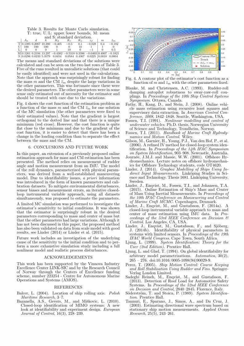
Table 3. Results for Monte Carlo simulation.T: true, U/L: upper/lower bounds, M: mean

and S: standard deviation.Ax d k Kδ Kr Kv zf m zm

T 0.1385 0.2067 10.380 −0.405 −0.5 0.1 −0.028 0.4 −0.182U 100 100 100 0 0 10 1 1 0L 0 0 0 1 10 0 −1 0 0.5

M 0.1261 0.2194 13.297 −0.4302 −0.5318 0.3396 −0.0403 0.4007 −0.1821S 0.0296 0.0233 5.3579 0.0454 0.0584 0.4367 0.0225 0.0018 0.0004

The means and standard deviations of the solutions werecalculated and can be seen on the two last rows of Table 3.Five of the runs resulted in unrealistic solutions (that couldbe easily identified) and were not used in the calculations.Note that the approach was surprisingly robust for findingthe mass m and the CM zm despite the large variations inthe other parameters. This was fortunate since these werethe desired parameters. The other parameters were in somesense only estimated out of necessity for the estimator andshould be treated with care due to the variations.Fig. 4 shows the cost function of the estimation problem asa function of the mass m and the CM zm for one solutionof the MC simulation (the other parameters were fixed totheir estimated values). Note that the gradient is largestorthogonal to the dotted line and that there is a uniqueminimum (red cross). However, the cost function is quiteflat close to the minimum and due to the gradient of thecost function, it is easier to detect that there has been achange in the loading condition than to separate the effectbetween the mass and the CM.

6. CONCLUSIONS AND FUTURE WORKIn this paper, an extension of a previously proposed onlineestimation approach for mass and CM estimation has beenpresented. The method relies on measurement of rudderangle and motion measurement from an IMU. The modelof the roll dynamics, parameterized with physical param-eters, was derived from a well-established maneuveringmodel. Due to identifiability issues, a priori informationwas introduced in the form of known parameters and cali-bration datasets. To mitigate environmental disturbances,sensor biases and measurement errors, an iterative closed-loop instrumental variable approach, using all datasetssimultaneously, was proposed to estimate the parameters.A limited MC simulation was performed to investigate theestimator’s sensitivity to initial conditions. It was shownthat the estimator is surprisingly robust in the desiredparameters corresponding to mass and center of mass butthat the other parameters had large variations. Although ithas not been discussed in this paper, the proposed methodhas also been validated on data from scale model with goodresults, see Linder (2014) or Linder et al. (2015).Future work includes an investigation of the underlyingcause of the sensitivity to the initial condition and to per-form a more exhaustive simulation study including a fullnonlinear model and realistic process disturbances.

ACKNOWLEDGEMENTSThis work has been supported by the Vinnova IndustryExcellence Center LINK-SIC and by the Research Councilof Norway through the Centers of Excellence fundingscheme, number 223254 - Centre for Autonomous MarineOperations and Systems (AMOS).

REFERENCESBalcer, L. (2004). Location of ship rolling axis. PolishMaritime Research, 3–7.

Bazanella, A.S., Gevers, M., and Miškovic, L. (2010).Closed-loop identification of MIMO systems: A newlook at identifiability and experiment design. EuropeanJournal of Control, 16(3), 228–239.

m [kg]0 0.1 0.2 0.3 0.4 0.5 0.6 0.7 0.8 0.9 1

7z m[m

]

-0.5

-0.45

-0.4

-0.35

-0.3

-0.25

-0.2

-0.15

-0.1

-0.05

0

Contour PlotTrenchmzm = mzm

Solution 0.05

0.1

0.15

0.2

0.25

0.3

0.35

0.4

0.45

Fig. 4. A contour plot of the estimator’s cost function as afunction ofm and zm with the other parameters fixed.

Blanke, M. and Christensen, A.C. (1993). Rudder-rolldamping autopilot robustness to sway-yaw-roll cou-plings. In Proceedings of the 10th Ship Control SystemsSymposium. Ottawa, Canada.

Fathy, H., Kang, D., and Stein, J. (2008). Online vehi-cle mass estimation using recursive least squares andsupervisory data extraction. In American Control Con-ference, 2008, 1842–1848. Seattle, Washington, USA.

Fossen, T.I. (1991). Nonlinear modelling and control ofunderwater vehicles. Ph.D. thesis, Norwegian Universityof Science and Technology, Trondheim, Norway.

Fossen, T.I. (2011). Handbook of Marine Craft Hydrody-namics and Motion Control. Wiley.

Gilson, M., Garnier, H., Young, P.J., Van den Hof, P., et al.(2006). A refined IV method for closed-loop system iden-tification. In Proceedings of the 14th IFAC Symposiumon System Identification, 903–908. Newcastle, Australia.

Journée, J.M.J. and Massie, W.W. (2001). Offshore Hy-dromechanics. Lecture notes on offshore hydromechan-ics for Offshore Technology students, code OT4620.

Linder, J. (2014). Graybox Modelling of Ships Using In-direct Input Measurements. Linköping Studies in Sci-ence and Technology. Thesis 1681. Linköping University,Sweden.

Linder, J., Enqvist, M., Fossen, T.I., and Johansen, T.A.(2015). Online Estimation of Ship’s Mass and Centerof Mass Using Inertial Measurements. In Proceedings ofthe 10th IFAC Conference on Manoeuvring and Controlof Marine Craft MCMC. Copenhagen, Denmark.

Linder, J., Enqvist, M., and Gustafsson, F. (2014a). Aclosed-loop instrumental variable approach to mass andcenter of mass estimation using IMU data. In Pro-ceedings of the 53rd IEEE Conference on Decision &Control. Los Angeles, CA, USA.

Linder, J., Enqvist, M., Gustafsson, F., and Sjöberg,J. (2014b). Identifiability of physical parameters insystems with limited sensors. In Proceedings of the 19thIFAC World Congress. Cape Town, South Africa.

Ljung, L. (1999). System Identification: Theory for theUser (2nd Edition). Prentice Hall.

Ljung, L. and Glad, T. (1994). On global identifiability forarbitrary model parametrizations. Automatica, 30(2),265 – 276. doi:10.1016/0005-1098(94)90029-9.

Perez, T. (2005). Ship Motion Control: Course Keepingand Roll Stabilisation Using Rudder and Fins. Springer-Verlag London Limited.

Sadeghi Reineh, M., Enqvist, M., and Gustafsson, F.(2013). Detection of Roof Load for Automotive SafetySystems. In Proceedings of the 52nd IEEE Conferenceon Decision and Control, 2840–2845. Florence, Italy.

Söderström, T. and Stoica, P. (1989). System Identifica-tion. Prentice Hall.

Tannuri, E., Sparano, J., Simos, A., and Da Cruz, J.(2003). Estimating directional wave spectrum based onstationary ship motion measurements. Applied OceanResearch, 25(5), 243–261.