IMU-based pose-estimation for spherical robots with limited resources

Jasper Zevering*, Anton Bredenbeck, Fabian Arzberger, Dorit Borrmann, Andreas Nuechter1

Abstract— Spherical robots are a robot format that is notyet thoroughly studied for the application of mobile mapping.However, in contrast to other forms, they provide some uniqueadvantages. For one, the spherical shell provides protectionagainst harsh environments, e.g., guarding the sensors andactuators against dust and solid rock. This is particularlyuseful in space applications. Furthermore, the inherent rotationthe robot uses for locomotion can be exploited to measurein all directions without having the sensor itself actuated. Areasonable estimation of the robot pose is required to exploitthis rotation in combination with sensor data to create aconsistent environment map. This raises the need for interpo-lating instances for calculation-intensive slow algorithms suchas optical localization algorithms or as an initial estimate forsubsequent simultaneous localization and mapping (SLAM).In such cases, inertial measurements from sensors such asaccelerometers and gyroscopes generate a pose estimate forthese interpolation steps.

The paper presents a pose estimation procedure based oninertial measurements, that exploits the known dynamics of aspherical robot. It emphasizes a low jitter to maintain constantworld measurements during standstill and avoids exponentiallygrowing error in position estimates. Evaluating the position andorientation estimates with given ground truth frames shows thatwe reduce the jitter in orientation and handle slip and partlyslide behavior better than other commonly used filters such asthe Madgwick filter.

I. INTRODUCTION

Spherical robots are a relatively narrow field of robotics.Still, they could be useful in situations where the measure-ment equipment needs to be protected against harsh envi-ronments. As an example, the 2021 CDF study LunarCavesby ESA about the feasibility of a spherical robot, calledDAEDALUS, for exploration of lunar-lava tubes [1] showsthe need for orientation and position estimation of sphericalrobots with the limitations on resources common for space-applications. Although a purely Inertial Measurement Unit(IMU)-based estimation is not recommended for variousreasons, the lack of an absolute reference among others,IMU-based pose estimation is used as part of an overallmulti-sensor-fusion-based estimation. IMUs are sensors withhigher refresh rates than Simultaneous Localization andMapping (SLAM) based algorithms, such as optical or LightDetection and Ranging (LIDAR) SLAM. This makes them

* Corresponding author:info@jasperzevering.de

1 All authors are with Informatics VII : Robotics and Telematics -University of Wuerzburg

We acknowledge funding from the ESA Contract No.4000130925/20/NL/GLC for the “DAEDALUS – Descent And Explorationin Deep Autonomy of Lava Underground Structures” Open SpaceInnovation Platform (OSIP) lunar caves-system study and the EliteNetwork Bavaria (ENB) for providing funds for the academic program“Satellite Technology”.

suitable for interpolating the more precise and absoluteposition reference points of these slower algorithms. Thelimited computational power of space-qualified CPUs furtherimposes the need for good orientation estimation with-out computational-intensive algorithms like Kalman filters.Lastly, the geometry of a spherical robot opens the possibilityfor the not often used position estimation by IMUs.

This paper introduces an IMU-based orientation and po-sition algorithm for spherical robots with limited compu-tational power and the need for real-time estimations. Thealgorithm does not rely on one specific locomotion approach,but it assumes a rotation of the IMU together with at least theshell of the robot, if not the whole robot. The experimentsin this paper use the setup of the IMUs of the prototypedepicted in Figure 1, which is inspired by previous worksuch as Daedalus [1]. Due to the lack of a locomotion system,the sphere needs to be rolled externally. A Livox Mid-100laser scanner was used for evaluation purposes. In additionto analying the filtered output the evaluation will show anddiscuss the resulting point clouds of this prototype with thepresented pose estimation.

II. ASSUMPTIONS AND PRELIMITATIONS

The presented approach works for any spherical robot withIMUs that moves based on rotation. Nevertheless, it requiresmultiple assumptions to be beneficial in comparison to ex-isting approaches. Some of these arise from the fundamentalbehavior of spherical robots and some more specific fromthe DAEDALUS project. The approach becomes beneficialgiven the following assumptions and requirements:

Fig. 1. Prototype to test the algorithm in an envisaged technical envi-ronment. The main payload is the Livox Mid-100 laser-scanner. For pose-estimation, three IMUs of the manufacturer Phidget are placed on the middleplate and a Raspberry Pi 4 for the calculations. On the top are two batteriesand on the bottom one voltage stabilizer and breakout box of the laser-scanner.

1. Real Time Operations: The operation of the robotrequires real time calculation of the pose. This implies theusage of onboard computational power.

2. Limitation of Computational Power: Due to the needfor efficient code without massive bottleneck operations, suchas matrix inversion in the extended Kalman Filter, the codemust minimize the usage of non-basic operations.

3. Low Costs of Hardware: We assume biased and noisydata in a non-negligible amount from the sensors.

4. Sphere Shape: The code relies heavily on the as-sumption of a spherical shape with a constant radius. Ac-cordingly, rotation on the ground leads to translation.

5. Slip and Sliding: We assume the sphere is affected byboth slip, i.e., the sphere rotates with no resulting translation,and sliding, i.e., the sphere may translate without rotating ina limited, non-permanent way. The limitation refers to theassumption that sliding and slipping reduce the amount oftranslation for a given rotation and vice versa, however, notfor complete absence.

6. Stability of Pose: For SLAM purposes using LI-DARs, a stable but maybe minimal false pose is preferredover a more exact but noisy and jumping position.

7. Further Processing of Pose: The approach shouldavoid jumping values or abrupt changes of data if notclearly indicated by the sensors. Suppose there is an internalalgorithmic change of behavior due to the change of statefrom standing to rolling. This change shall not be representedby an unnatural acceleration in the data.

8. Uncertainty of Iterative Position Integration: IMUsdeliver no absolute reference for a position as they do fororientation in the form of a noisy but measurable gravityvector. So without external or secondary sensors relyingon absolute waypoints, the position estimation will alwaysunderlie the integration of errors.

9. Space Suitability: As the algorithm is considered tobe applied for space missions, the magnetometer data is notconsidered in the algorithm, despite its positive impact onorientation estimation on Earth.

10. Short Term Mobility: The approach is targeted ata spherical robot for data collection with a laser scanner,requiring standstill periods for scanning. In further extension,the fusion of a pose estimation by the laser scanner willbe merged. Thus, the sphere is considered to move inmultiple short paths and not roll continuously for a longperod. Relying on integration parts, the IMU-based algorithmbenefits from this assumption.

11. Non-reliability of locomotion commands: ForDAEDALUS, the same input of the locomotion controllerleads to heavily different behaviors depending on the pose ofthe robot and the surface structure [1]. Also, the DAEDALUSrobot has two utterly different locomotion methods; there-fore, we will not take locomotion itself, nor the controllerinput or output into account for pose estimation.

We conclude that the generated data has to be a com-promise between simple on-board filtration of data, whilestill being usable for heavy calculation post-record, e.g. mapgeneration. It has to be easy to calculate and adapt to the

specific needs. Making assumptions about the dynamics ofthe system, it must nevertheless deliver reliable estimateswhich take physical behavior into account. It shall be real-time capable and does not rely on delayed steps. Theresulting algorithm is restricted to spherical or cylindricalrobots. It is optimized for gathering laser data where noisypose estimates while standing deteriorate the map creationprocess, and therefore, even if slightly false, a stable positionis preferred.

III. STATE OF THE ART

For pose estimation on embedded hardware, there are threemain algorithms.

A. Kalman Filter

The Kalman Filter or the more suitable Extended KalmanFilter (EKF) use state prediction and correction based onsensor data for orientation estimation [2]. For the definedlimitations, the Kalman Filter is not suitable. First, the EKFrequires a considerable amount of computational power,mainly due to matrix inversion. For this, the needed calcula-tions grow exponentially with input data. Further, the KalmanFilter relies on input to a system to calculate an estimationof the pose for the next iterative step. But, as described inSection II, we cannot take the input to locomotion controlas a reference for pose estimation as the behavior is notlinear or even predictable without exact knowledge of thesurface. Therefore it is not possible to implement a physicalbehavior of the system to the filter, as easily as it is forother robotic applications. The Error State Extended KalmanFilter, which works solely with IMU data [3], requiressubstantial computational power. For the later introducedposition estimation for spherical robots, some calculationsare used for the orientation as well as for the position. Afterall, if computational power is not limited, Kalman Filtersprovide principally better results.

B. Madgwick Filter

The Madgwick filter is a widely used filter for orientationestimation with IMUs [4]. It is efficient and easy to calculatebut does not consider the physics of the motion. It uses agradient descent algorithm. It nearly provides the sought-after classification for the orientation. The behavior is shownin comparison to the complementary filter in Figure 2.Being optimized for movement the Madgwick filter has ajittering behavior at the standstill of the IMU. This does notmeet the desired behavior as described in the prelimitationsSection (II). As we do not use a magnetometer, we cannotuse the gyro bias estimation of the Madgwick filter.

C. Complementary Filter

A complementary filter is a fundamental approach ofcombining precise but not exact with non-precise but exactdata. Therefore it is widely used for combining noisy ac-celerometer data with gravity as a reference with the precisebut drifting measurement of gyroscopes. The basic conceptis to have the main part of a value dominated by a gyroscope

0 1 2 3 4 5

-2

0

2

q0

10-3

0 1 2 3 4 5

-2

0

2

q1

10-3

0 1 2 3 4 5

-2

0

2

q2

10-3

0 1 2 3 4 5

-2

0

2

q3

10-3

Madgwick (gain 0.2)

Complementary (gain 0.02)

Time in s

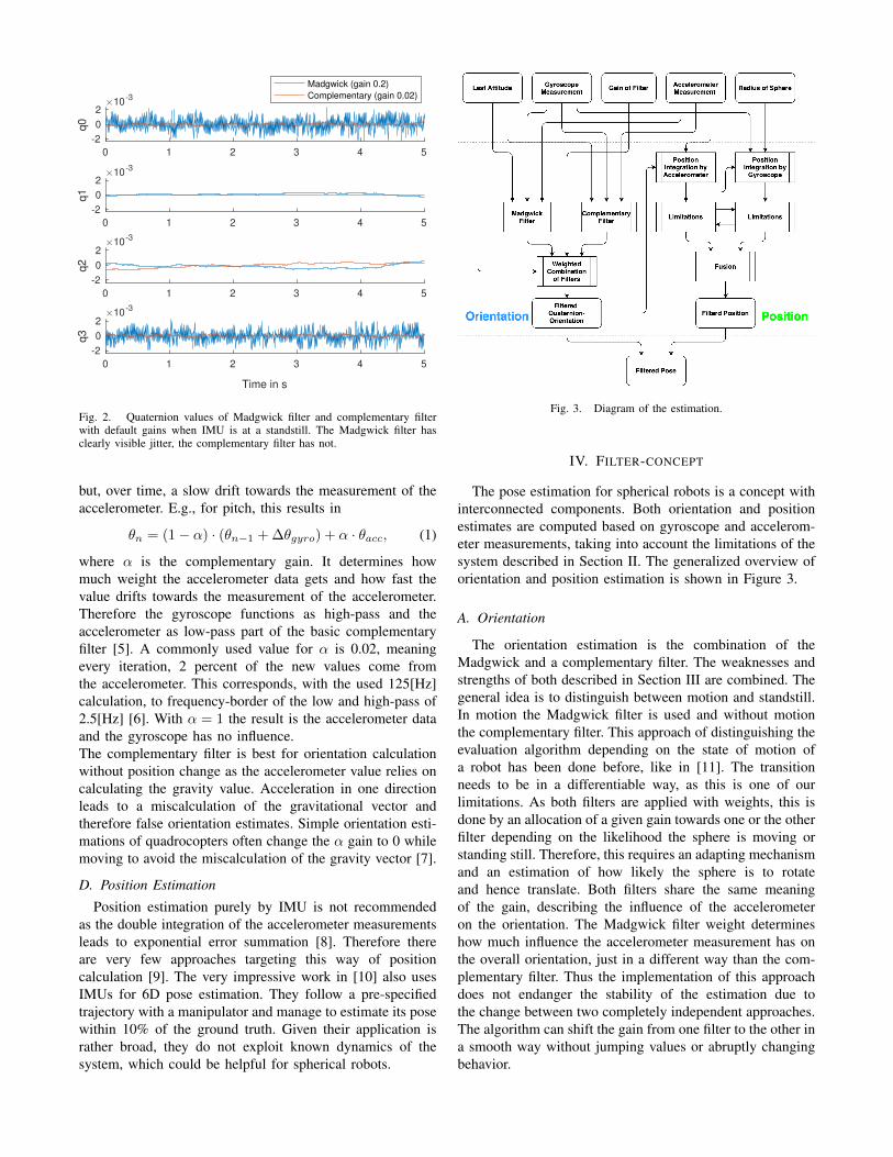
Fig. 2. Quaternion values of Madgwick filter and complementary filterwith default gains when IMU is at a standstill. The Madgwick filter hasclearly visible jitter, the complementary filter has not.

but, over time, a slow drift towards the measurement of theaccelerometer. E.g., for pitch, this results in

θn = (1 − α) · (θn−1 + ∆θgyro) + α · θacc, (1)

where α is the complementary gain. It determines howmuch weight the accelerometer data gets and how fast thevalue drifts towards the measurement of the accelerometer.Therefore the gyroscope functions as high-pass and theaccelerometer as low-pass part of the basic complementaryfilter [5]. A commonly used value for α is 0.02, meaningevery iteration, 2 percent of the new values come fromthe accelerometer. This corresponds, with the used 125[Hz]calculation, to frequency-border of the low and high-pass of2.5[Hz] [6]. With α = 1 the result is the accelerometer dataand the gyroscope has no influence.The complementary filter is best for orientation calculationwithout position change as the accelerometer value relies oncalculating the gravity value. Acceleration in one directionleads to a miscalculation of the gravitational vector andtherefore false orientation estimates. Simple orientation esti-mations of quadrocopters often change the α gain to 0 whilemoving to avoid the miscalculation of the gravity vector [7].

D. Position Estimation

Position estimation purely by IMU is not recommendedas the double integration of the accelerometer measurementsleads to exponential error summation [8]. Therefore thereare very few approaches targeting this way of positioncalculation [9]. The very impressive work in [10] also usesIMUs for 6D pose estimation. They follow a pre-specifiedtrajectory with a manipulator and manage to estimate its posewithin 10% of the ground truth. Given their application israther broad, they do not exploit known dynamics of thesystem, which could be helpful for spherical robots.

Fig. 3. Diagram of the estimation.

IV. FILTER-CONCEPT

The pose estimation for spherical robots is a concept withinterconnected components. Both orientation and positionestimates are computed based on gyroscope and accelerom-eter measurements, taking into account the limitations of thesystem described in Section II. The generalized overview oforientation and position estimation is shown in Figure 3.

A. Orientation

The orientation estimation is the combination of theMadgwick and a complementary filter. The weaknesses andstrengths of both described in Section III are combined. Thegeneral idea is to distinguish between motion and standstill.In motion the Madgwick filter is used and without motionthe complementary filter. This approach of distinguishing theevaluation algorithm depending on the state of motion ofa robot has been done before, like in [11]. The transitionneeds to be in a differentiable way, as this is one of ourlimitations. As both filters are applied with weights, this isdone by an allocation of a given gain towards one or the otherfilter depending on the likelihood the sphere is moving orstanding still. Therefore, this requires an adapting mechanismand an estimation of how likely the sphere is to rotateand hence translate. Both filters share the same meaningof the gain, describing the influence of the accelerometeron the orientation. The Madgwick filter weight determineshow much influence the accelerometer measurement has onthe overall orientation, just in a different way than the com-plementary filter. Thus the implementation of this approachdoes not endanger the stability of the estimation due tothe change between two completely independent approaches.The algorithm can shift the gain from one filter to the other ina smooth way without jumping values or abruptly changingbehavior.

B. Position

As there is no absolute reference of position neither withcalculation by gyroscope nor by the accelerometer, the filtercan only try to improve the calculation of the velocity leadingto the change in position. The straightforward approach is todouble integrate the accelerometer, which leads to the earlierdescribed unwanted behavior of exponential error integrationand makes the position estimates completely unusable.

An alternative approach multiplies the rotation speed withthe known radius of the sphere and takes this as velocity,integrating once. The more precise and less noisy data ofthe gyroscope leads to usable position estimates. There isno such extensive error integration, and more importantly:no exponentially growing error with time. However, if thesphere slips, this approach will predict the full translation.Also, if there is translation but just slight rotation becauseof sliding, it will predict too little translation. Furthermore,integrating the rotation does not let us estimate verticalmovement. Thus, this approach neglects potential slip andsliding (limitation 5) as well as vertical movement. Everyrotation will be predicted as translation in a given plane,which is most likely parallel to the ground. For instance,if the sphere rolls up an obstacle, the length of the path isestimated to be the ground-plane.

Our algorithm combines both approaches of position es-timation and limits all components according to the othercomponents. This implies a connection between translationand rotation. Overall the extreme situation (full translation,no rotation, or the other way round) will automatically leadto wrong predictions, as there is no way to tell which ofthe two approaches has at that moment more reliable data.Therefore, the combination of both rather than only one ischosen.

V. FILTER-IMPLEMENTATION

A. Orientation

The orientation is a symbiosis of the Madgwick filter andcomplementary filter. The complementary filter is chosenfor no or slow motion, the Madgwick filter for fast mo-tion. The Madgwick filter itself is untouched. The standardcomplimentary filter works with Euler angles (roll, pitch,yaw (RPY)) resulting from the direct integration of thegyroscope while the Madgwick filter outputs quaternions.Quaternions were designed under the premise of beingfree from singularities, i.e., for a continuous change inorientation, there exists a continuous change in quaternionrepresentation [12]. This is not the case for Euler angles,as a transition of a 359-degree roll to a 0-degree roll hasno continuous value representation if limited to 360 degrees.Updating the orientation for the complementary filter impliesa transition of each angle independently. Combining bothrepresentations leads to contradicting updates from each filterwith respect to the other. Thus, the complementary filter isadapted to work in quaternion representation. Hence, theRPY-orientation is transformed to a quaternion, and thena quaternion slerp is performed [13]. The quaternion slerp

utilizes the representation of two quaternions on a sphere.The transition from one quaternion to the other is not donedirectly but always over the surface of the sphere. This leadsto the same handling of quaternions as the Madgwick-filterwithout endangering robustness due to using two differentquaternions with very different values representing nearlythe same position.

The transition between the two filters is done by shiftinga fixed factor among the α-gain of the complementary filterand the gain factor of the Madgwick filter. As the commonvalues widely used for both values differ by one order ofmagnitude, the gain shifted to the complementary filter isdivided by ten and the other way around. The values ofthe gyroscope axes determine in which manner to shift theoverall gain to both filters. The defining values are the twothresholds for using solely the complementary filter on theone hand or a full Madgwick filter on the other hand. Thesevalues have been determined empirically. Future work willinvestigate improving those values by developing a suitableheuristic for the thresholds. The transition between the fullcomplementary and the full Madgwick estimation, as isrequired by the prelimitations, can be done by a function suit-able for the specific scenario. This avoids large accelerationsof the orientation due to the rapid change from one algorithmto another. In our experiments, when starting from standstill,the incipient Madgwick filter has a more rapid impact onthe orientation values than the incipient complementary filterwhen stopping rotation. Therefore the transition between α-gain of the complementary filter and the Madgwick-gain waschosen to have quadratic behavior. The value referred to asautogain Θ indicates how much impact both employed filtershave on the orientation estimation. Therefore we calculatefactors from the gyroscope measurements and scale theautogain with the maximum β (cf. equation 2 and 3). gkrepresents the gyro measurement in the corresponding axisk, in rad/s. Later on, these factors will again be used forposition estimation, namely to determine if the sphere rotatesor not. These factors are heuristically defined as:

fk =

0 gk ≤ 0.1

0.25 · (gx − 0.1)2 0.1 < gk < 2.1

1 gk ≥ 2.1

, (2)

β = max(fx, fy, fz). (3)

Then the Madgwick gain γ for a given autogain Θ iscalculated by

γ = Θ · β. (4)

The complementary filter gain α is calculated by

α = Θ · θ · (1 − β). (5)

Thus, the Madgwick gain has a maximum of Θ and α amaximum of θ · Θ. This ratio θ can be adapted to specificneeds. We used θ = 0.1 as the ratio between the two often

used standard values γ = 0.2 and α = 0.02. Hence foradapting the position estimation to a given robot, the functionfor calculating the factors needs to be adapted in such a waythat it is a good indication for movement or standstill. Theratio θ needs to be chosen in a way that the desired ratiobetween Madgwick and complementary gain is reached. Andlastly, the autogain needs to be chosen to fit the specificneeds in terms of how strong both filters should be ableto influence the orientation. We used Θ = 0.2 to get thedescribed common values.

B. Position

The calculated orientation is directly used for positioncalculation. With the orientation, a gravity vector is calcu-lated, which, once normalized, represents the measurementof the accelerometer in abstinence of movement. Let g =[0 0 −1

]Trepresent the gravity vector in the world frame

and the matrix R represent the current orientation of theIMU, then

g′ =

g′xg′yg′z

= R ·

00−1

(6)

describes the effect of gravity in the coordinate system ofthe IMU. This gravity vector is then subtracted from theaccelerometer measurement. If there is no translation, thesubtraction should lead to

[0 0 0

]Tmeaning there is

no acceleration other than gravity. If there are non-zerocomponents, there is an acceleration in that direction. Giventhe accelerometer measurement a this leads to the velocityvector vxAcc

vyAccvzAcc

=

∫ T

0

axayaz

−

g′xg′yg′z

dt. (7)

These values are now coupled to the rotation of both axesother than their own. Therefore, the factors from the orien-tation step, representing the likelihood of rotation, are usedas limiting factors:vxAccL

vyAccLvzAccL

=

vxAccvyAccvzAcc

·

max(fy, fz)max(fx, fz)max(fx, fy)

. (8)

If one of the three factors is 1, this means there is atranslation in this direction. When there is no rotation, itwill set the velocity to 0. During fast motion, this allowsexponential error integration. This exponential error is takencare of later on.

The rotation into the world frame is computed as:vxAccWorldvyAccWorldvzAccWorld

= RT ·

vxAccLvyAccLvzAccL

. (9)

The next step requires the velocity calculated by the rotation.Therefore the rotations (direct values from the gyro) arerotated into the world frame: ωxWorld

ωyWorld(ωzWorld)

= RT ·

gxgygz

. (10)

The rotation around the world z-axis is not used to calculatethe velocity. Its effect on the position is considered whendetermining the orientation in the world coordinate system.ωzworld does not need to be computed as it has no influenceon the position.

The resulting velocities are calculated by multiplying thecircumference of the sphere:[vxzGyroWorldvyzGyroWorld

]=

[ωyWorld/(2π)ωxWorld/(2π)

]·2πr =

[ωyWorldωxWorld

]·r , (11)

where r is the radius of the sphere. As the gyro mea-sures rad/s the value is divided by 2π. Note that the two-dimensional velocities vxzGyroWorld and vzzGyroWorld do notcorrespond to the velocity on the ground plane but mayconsist of motion in z direction.

Next, the vxAccWorld and vyAccWorld are limited dependingon vxzGyroWorld and vyzGyroWorld. In our experiments, this was120 percent of the gyro calculated velocity. This ensures noexponential error integration when in motion. This is coupledto the physical act of sliding. The higher the likelihood ofsliding, the higher the velocity should be compared to thevelocity based on rotation. This does not count for slipping,as this implies the adaption of limitation of the velocityby rotation by the velocity measured by the accelerometer.But there is no need for a limitation as there is no doubleintegration with the rotation.The last step for calculating the velocity is taking the velocityin z-direction into account for the velocity by rotation. Thisvelocity in z is from the noisy double integration, as this isthe only indication for change of the z-axis. To avoid largeerrors and unlimited double error integration, vzAccWorld islimited to the mean of vxzGyroWorld and vyzGyroWorld. With thePythagorean theorem the velocity in x and y is calculatedaccepting the velocity in z-direction, which cannot be derivedby the velocity from gyro:[

vxGyroWorldvyGyroWorld

]=

√v2xzGyroWorld − v2zAccWorld√v2yzGyroWorld − v2zAccWorld

. (12)

The last step to get the position is the integration of thevelocity:pxpy

pz

=

∫ T

0

(1 − β)vxAccWorld + β · vxGyroWorld(1 − β)vyAccWorld + β · vyGyroWorld

vzAccWorld

dt.(13)

Depending on the practical circumstances and quality ofmeasurement, the factor β determines whether the positionrelies more on the accelerometer calculated velocity or thegyro. There should always be a mixture of both if there isslipping and sliding. β = 0.5 results in the mean of bothapproaches.

6 8 10 12 14 16 18 20 22

Time in s

-1

-0.8

-0.6

-0.4

-0.2

0

0.2

0.4

0.6

0.8

1Q

uate

rnio

n v

alu

eAutogain 0.2

Only Madgwick 0.2

Fig. 4. Quaternion-values of the presented fusion of complementary andMadgwick filter and only the Madgwick filter.

C. Time Complexity

Overall a pose estimation step consists only of operationsthat are constant in time. Given that we use the fast inversesquare root algorithm [14] for normalization, the trigono-metric functions are considered the remaining bottleneck.Overall there are 14 trigonometric function calls (4×arctan,4× sin, 4× cos, 1×arcsin, 1×arccos) and 5 divisions. TheIMU measurements are collected at 125 Hz and are processedwithout problems on a raspberry pi. Hence no overwhelmingcomputational load is to be expected.

VI. EVALUATION

The proposed algorithm is evaluated by two sets of exper-iments performed with three Phidgets 3/3/3 IMUs mountedon a circular acrylic glass plate with a diameter of 29 cm.For position experiments, the plate is put inside an acrylicglass sphere with the same radius as the glass plate. First, thefusion of Madgwick and complementary filter, here denotedas Autogain, is compared to a Madgwick only estimate.Second, the trajectory computation using both gyroscope andaccelerometer is evaluated.

A. Orientation

A first experiment is performed to show the overall per-formance of the Autogain computation for the orientation.The IMU was manually rotated in arbitrary directions, andthe orientation was plotted using the Madgwick filter andthe Autogain filter. As expected, the overall behavior ofthe presented algorithm and the Madgwick filter is verysimilar in the dynamic case, as shown in Figure 4. The moreexpressive part is the change between motion and standstill,as in motion, both filters use the same algorithm but differduring standstill and slow motion. As described in SectionIII, the Madgwick filter has a rather strong jitter during slowmovements and standstill. This is due to the (too) large stepsof gradient descent iterations. To compensate for this, oneneeds to lower the gain, leading to more imprecise resultsduring movement, as large iteration steps are beneficial there.Alternatively, one needs to increase calculation frequency,

0 2 4 6 8 10 12

Time in s

0

0.5

1

1.5

2

2.5

3

3.5

Dis

tance in d

eg

Autogain 0.2

Madgwick 0.2

Fig. 5. Distance of the proposed and the Madgwick algorithm to the opticaltracking system, using the distance definition of [15].

which is in our scenarios limited by the hardware capabilitiesof the IMU.

To evaluate specifically the change between slow motionand standstill, a further experiment is performed. Figure 5shows the distance to a precise external reference over ashort excerpt of the experiment with three phases of slowmotion and rotation at second 7, 9 and 11. For externalreference, we used a precise optical tracking system. Thedefinition and proposed calculation of the distance of 2quaternions of [15] was used. It describes the direct anglebetween two quaternions. The optical system matches theoverall orientation of both IMU-based algorithms quite welland lacks the perturbations of the pure Madgwick filter.The transformation of the orientation by the optical trackingsystem and the IMU-based algorithms yield two unknowntransformations, the relative orientation of the coordinatesystem of IMU to the optical coordinate system and how theaxes are interpreted on the tracked structure itself. Therefore,the algorithm proposed in [16] was used to solve these twounknown transformations on basis of the resulting data, tomatch the orientations of optical and IMU-based data. As thismatching of the optical system happens on basis of one of thetwo IMU orientation data-sets, the comparison of absolutedifferences may be misleading, as the transformations werematched on basis of the autogain filter. To stress the jitterbehavior of the Madgwick without relying on absolute orien-tation, which will be part of further research, Figure 6 showsthe derivative of the distance. Here the change of directiondue to small oscillations and the smoother fusion algorithmin comparison to the tracking is even more apparent.

B. Position

The primary evaluation for the position focuses on slip-and slide-behavior. Here the plate with the IMU(s) is fixedinside a sphere with a diameter of 29 cm and rolled along an“L”-shaped track of one meter by one meter. Slip behaviorwas manually provoked. Figure 7 shows the resulting trajec-tories. Pure rotation integration leads to an enlarged “L” by

0 2 4 6 8 10 12

Time in s

-0.6

-0.4

-0.2

0

0.2

0.4

0.6

0.8

1C

hange o

f dis

tance in d

eg/s

Autogain 0.2

Madgwick 0.2

Fig. 6. Derivative of the distance of the proposed and the Madgwickalgorithm to the optical tracking system, using the distance definition of[15].

-1 -0.5 0 0.5

x in m

-2.6

-2.4

-2.2

-2

-1.8

-1.6

-1.4

-1.2

-1

-0.8

y in m

1.13

1.47

1.52

0.93

Fusion-Algorithm

Only rotation integration

Fig. 7. Ground position (Z-axis, perpendicular to the ground) by integrationof rotation and the fusion algorithm. An L-shape with 1 m by 1 m wasperformed with provoked slip (rotation without translation). For referencesthe boxes are manually set points with the distance in meter between thesepoints written on the lines connecting them. The rolling started in the upperright corner and ended in the bottom left corner.

about 50 percent, as the manually provoked rotation is justintegrated and therefore interpreted as linear motion. Thefusion between the accelerometer and gyroscope interpretsan “L” with dimensions much closer to the original. Theestimation leaves room for improvement, as in one direction,it misses the actual length about -10 percent, and in the otherdirection overestimates it by 10 percent. But it shows theoverall capability of the algorithm to compensate for slip.

The same experiment was performed with added slide,i.e., more translation than just the rotation produces. Herethe results shown in Figure 8 were not as reliably good aswith the slip experiment. This is due to the timing of theacceleration. In order to recognize the acceleration as trans-lation, the rotation needs to be above a certain threshold, as

-1.2 -1 -0.8 -0.6 -0.4 -0.2 0

x in m

-0.1

0

0.1

0.2

0.3

0.4

y in

m

1.02

0.81

0.480.46

Fusion-Algorithm

Only rotation integration

Fig. 8. Ground position (Z-axis, perpendicular to the ground) by integrationof rotation and the fusion algorithm. An L-shape with 1 m by 1 m wasperformed with provoked slide(translation without rotation). For referencethe boxes are manually set points with the distance in meter between thesepoints written on the lines connecting them. The rolling started in the lowerright corner and ended in the upper left corner.

the algorithm does not allow any translation without rotationat all. The translation is computed using the accelerometervia double integration. Therefore the acceleration of the slidemovement needs to be at the same time as a minimal amountof rotation. If the rotation starts after the sliding, the doubleintegration of the acceleration is suppressed. When therotation starts and the translation could be double integrated,it is already zero as the velocity is constant. This can beseen in Figure 8 where the one side of the L was interpretedexactly as long as the pure integration, i.e., approx. 50 cm,and therefore the slide was not recognized, and the otherpart was correctly interpreted longer than just the integrationand with 1.02 m as long as the actual trajectory. This is tobe blamed on the execution of the experiment, as it was notperfectly ensured only to start sliding with ongoing rotation,which is hard to achieve when manually guiding a sphere.However, the sliding behavior in a real environment couldbe in both ways, too, so sliding while rolling and startingsliding before rolling. With slip, this is not a problem, as,by definition, the translation cannot begin before the rotationwhen slipping. If so, it would be sliding. The experimentsfor sliding did not reliably detect the slide event and, onsome occasions, interpreted the distance as shorter than justthe integration, as the acceleration of the linear motion wasmissed. However, the deceleration of the sphere was stillrecognized while rotation existed, and therefore, the spheremiscalculated a couple of centimeters.

C. Impact on 3D mapping

One major design driver for the presented algorithm isthe suitability for spherical SLAM purposes. Therefore, apose estimate is preferred to be slightly wrong, if it is morecontinuous, i.e. less noisy and with less jumping values, thanthe exact pose has.

Fig. 9. Left: resulting 3D map using the presented algorithm for posefiltering. Right: resulting 3D map using Madgwick + double integrator forpose filtering. Both images were shot from the exact same point of view.Both plots use the same LIDAR data and apply one of the simultaneouslygenerated pose estimations.

To test the impact of the filter on 3D mapping, we used theprototype in Figure 1. After 2 s of initial standstill, the sphererolled approx. 4 m within 5 s in an indoor environment fromone corner of the room to the opposing one. We extractedthe laserscan data, as well as the filtered pose using thepresented algorithm. Without further pre- or post-processing,the pose data is combined with the laserscan data to createa 3D map. Figure 9 compares the result with another 3Dmap, using the pose estimation by the Madgwick filter andsimple rotation integration on the same data. Therefore thesame laserscan data is mapped with different pose estimates.The presented filter improves the resulting map comparedto the Madgwick/integrator approach. In particular, the wallsand the ceiling are more recognizable, which is favorable formany SLAM algorithms. Another improvement is that pointswere no longer sensed below the ground, i.e. the plane onwhich the sphere was moving on. The more detailed partof the map, as seen in the bottom left corner of the aboveimage of Figure 9, corresponds to the initial standstill. Itis more detailed than the rest of the map because of thenon-repeating flower-shaped scanning pattern, where pointdensity increases with time. Note that the same detailed partis also present in the right image. However, it is out of view(at the bottom right corner) as the Madgwick filter missesthe initial pose estimation by a lot.

D. Conclusion

This paper introduced an IMU-based pose estimation filterbased on the fusion of multiple already existing filters andapproaches. It is optimized for specific needs and circum-stances of spherical robots with laser scanning tasks in aspace-suitable way. Needless to say, a lot of work remainsto be done. The fusion of complementary and Madgwick ori-entation filter solves the shortcomings of the Madgwick filterwhen at a standstill, particularly the jitter. A first qualitativeevaluation shows the functionality of the filter. In furtherexperiments, a quantitative orientation comparison with asynchronized optical system needs to be performed. Also,as further work, all puzzle pieces, this filter, a locomotionsystem, a scanning system need to be combined to an overallworking prototype.

The presented position estimation shows the capability to

overcome the problem of the missing absolute reference ofIMUs partly. It mainly improves the measurements in theground plane with slip behavior present. Still, there is a needfor parameter tuning. Sliding was not all the time detectedreliably. Here a mechanism for a delayed rotation needs tobe investigated, that acceleration shortly before a rotation isintegrated and taken into account once rotation starts. Theapproach for, at least roughly, indicating the change in thez-direction, which is now done only by the accelerometervalues, shows no promising results nor usable results infirst qualitative experiments with rolling over obstacles andtherefore needs to be re-investigated.

REFERENCES

[1] Angelo Pio Rossi, Francesco Maurelli, Vikram Unnithan, HendrikDreger, Kedus Mathewos, Nayan Pradhan, Dan-Andrei Corbeanu, Ric-cardo Pozzobon, Matteo Massironi, Sabrina Ferrari, et al. Daedalus-descent and exploration in deep autonomy of lava underground struc-tures: Open space innovation platform (osip) lunar caves-system study.2021.

[2] Rudolph Emil Kalman. A new approach to linear filtering andprediction problems. Transactions of the ASME–Journal of BasicEngineering, 82(Series D):35–45, 1960.

[3] Mohammad Ahmadi, Alireza Khayatian, and Paknush Karimaghaee.Orientation estimation by error-state extended kalman filter in quater-nion vector space. In SICE Annual Conference 2007, pages 60–67.IEEE, 2007.

[4] Sebastian Madgwick. An efficient orientation filter for inertial andinertial/magnetic sensor arrays. Report x-io and University of Bristol(UK), 25:113–118, 2010.

[5] Hyung Gi Min and Eun Tae Jeung. Complementary filter design forangle estimation using mems accelerometer and gyroscope. Depart-ment of Control and Instrumentation, Changwon National University,Changwon, Korea, pages 641–773, 2015.

[6] Szabolcs Hajdu, Sandor Tihamer Brassai, and Iuliu Szekely. Com-plementary filter based sensor fusion on fpga platforms. In 2017International Conference on Optimization of Electrical and ElectronicEquipment (OPTIM) & 2017 Intl Aegean Conference on ElectricalMachines and Power Electronics (ACEMP), pages 851–856. IEEE,2017.

[7] Robert Mahony, Tarek Hamel, and J-M Pflimlin. Complementary filterdesign on the special orthogonal group so (3). In Proceedings of the44th IEEE Conference on Decision and Control, pages 1477–1484.IEEE, 2005.

[8] YK Thong, MS Woolfson, JA Crowe, BR Hayes-Gill, and DA Jones.Numerical double integration of acceleration measurements in noise.Measurement, 36(1):73–92, 2004.

[9] Manon Kok, Jeroen D Hol, and Thomas B Schon. Using iner-tial sensors for position and orientation estimation. arXiv preprintarXiv:1704.06053, 2017.

[10] J-S Botero Valencia, M Rico Garcia, and J-P Villegas Ceballos. Asimple method to estimate the trajectory of a low cost mobile roboticplatform using an imu. International Journal on Interactive Designand Manufacturing (IJIDeM), 11(4):823–828, 2017.

[11] Joachim Hertzberg, Kai Lingemann, and Andreas Nuchter. MobileRoboter: Eine Einfuhrung aus Sicht der Informatik, page 145. SpringerBerlin Heidelberg, Berlin, Heidelberg, 2012.

[12] Richard Becker. Dealing with the quaternion antipodal problem foradvecting fields. Technical report, US Army Research Laboratory USArmy Research Laboratory United States, 2017.

[13] Erik B Dam, Martin Koch, and Martin Lillholm. Quaternions,interpolation and animation, volume 2. Citeseer, 1998.

[14] Origin of quake3’s fast invsqrt(). beyond3d.com/content/articles/8/. Accessed: 2021-05-01.

[15] James J Kuffner. Effective sampling and distance metrics for 3d rigidbody path planning. In IEEE International Conference on Roboticsand Automation, 2004. Proceedings. ICRA’04. 2004, volume 4, pages3993–3998. IEEE, 2004.

[16] Fadi Dornaika and Radu Horaud. Simultaneous robot-world andhand-eye calibration. IEEE transactions on Robotics and Automation,14(4):617–622, 1998.