Modeling Flow through a Normal and Calcified Coronary

Artery

BME 429 Fluids Module Report Lab Group 5

Alex Thomason, Sarea Recalde Phillips, Thaddeus Schlamb

This lab investigates the hemodynamics of a normal and diseased coronary artery through

simulation and experimentation. The diseased artery experiences calcification around the

artery wall, decreasing the diameter of the artery creating a stenosis that affects blood flow

through the artery. Normal and calcified coronary arteries were extracted from patient

specific MRI images through Mimics. Through the use of COMSOL, particle visualization

flow was modeled and compared in both arteries. To validate the COMSOL fluid flow

models, hollowed arteries were created in 3Matics and 3D printed for benchtop testing.

The results of the particle tracing were based off the results of a time-dependent laminar

flow physics study that gave us the velocity profile through the normal and diseased model.

Hollow 3D models of the diseased and normal coronary arteries were printed and polished

so a dyed fluid with similar viscous properties of blood could be pumped through the

models. The fluid was pumped at the same velocity and pressure that was used in the

COMSOL simulations to provide consistency of boundary conditions. The fluid flow was

videotaped to capture how the fluid flowed through the diseased and normal arteries. Flow

through the benchtop experiment was similar to the COMSOL model, validating the

computational simulation.

Keywords - Coronary artery, stenosis, calcification, COMSOL, Mimics, CVD,

hemodynamic

I. Introduction

Cardiovascular disease (CVD), which narrows

blood vessels, causes strokes, heart attacks, and

various other heart maladies. This medical malady

is a growing concern across the world. In America

alone, 11.5% or 27.6 million adults have some form

of heart disease. In America the mortality rate has

become 221.9 per 100,000 afflicted with CVD. [1]

While over 7 million people in the United Kingdom's

are affected with CVD; with a new death every 8

minutes. [2] CVD can be prevented by reducing risk

factors, and by improving one’s diet and exercise

regiment. [3] Yet, CVD is currently irreversible, so

while preventable measures are important the

effects of the disease must be studied.[4]

The most common variation of CVD is coronary

artery disease, which can go without detection until

a heart attack. [5] Coronary artery disease occurs

when low-density lipoprotein (LDL) cholesterol

adhere to the vascular wall near areas of high shear

stress and turbulent flow. Behind the vascular wall,

macrophages consume the LDL cholesterol and

converts it to a foam cell. These foam cells thicken

with time into plaque starting the stenosis in the

artery. [6] As the stenosis grows it can constrict

blood flow leading to a heart attack. In addition, if

the pressure and shear stress is large enough the

vascular walls can rupture, allowing plaque to enter

blood flow and potentially damaging blood cells and

creating a blockage leading to a stroke. [7]

There are various methods to treat and manage

coronary artery disease. This includes medications

such as angiotensin-converting enzyme (ACE)

inhibitors, which dilates the blood vessels and

reduces high pressure gradients in the coronary

artery. [8] The more severe treatments include

coronary bypass surgery and balloon angioplasty

surgery. Coronary artery bypass grafting is when an

exterior vein is applied around the stenosis

improving blood flow while reducing pressure near

the stenosis.[9] Coronary angioplasty surgery is

when a catheter is positioned within the stenosis,

and a balloon inflates and compresses the stenosis.

A stent is placed in the reduced stenosis to

preventing decompression. [10] With the severity of

treatments and its high mortality rate coronary

artery disease has become a central point of

biomedical research.

Recently, efforts have been centralized around

modeling fluid flow paths within the cardiovascular

system. Until the advancements in computational

modeling, most fluid studies were restricted to

benchtop animal models or artificial models. With

the new use of computer modeling and its inherent

ability to solve complex differential equations

through finite element analysis, complex

hemodynamic studies can be solved. This allows

for improved fluids research in complex vessel

designs and potential treatments. This improved

computational method saves time and money

before a single prototype is produced. Therefore,

our concern for this project centered around

validating our computational model.

This fluid module began by extracting normal and

diseased models of two different coronary arteries

from two different MRI images in Mimics. The

purpose of this was simply to establish a 3D model

of each both arteries. It was important to obtain an

accurate model of the diseased artery with a visible

stenosis due to calcifications. In theory, the normal

artery model should have a clear path for blood

flow. After a rough model is obtained, it can be

smoothed using a wrapping tool, which will help

yield more accurate results later in the module.

Once the models were obtained in Mimics, they

were imported to 3Matics. The solid models were

smoothed, remeshed, and processed to import to

COMSOL. Additionally, secondary models of the

diseased and healthy arteries were hollowed and

remeshed to be 3D printed for benchtop

experimentation.

Once the solid models of the normal and

diseased arteries were meshed properly, they were

imported to COMSOL. The purpose of the

COMSOL simulations was to complete two, time-

dependent physics studies (laminar flow and

particle tracing) for the normal and diseased artery.

The laminar flow study yielded the velocity and

pressure profiles for both models as the fluid flowed

from the inlet to the outlet. The particle tracing study

used the results from the laminar flow study to trace

3,000 particles through the diseased stenosis and

normal model.

Each member’s diseased stenosis model of the

coronary artery was 3D printed so that a physical

experimental study could be performed to compare

the results of the particle tracing to the actual flow

in the 3D printed hollow models. In total the group

had three diseased models and one provided

normal hollow model to test.

After completion of the simulation, the benchtop

experiment was prepared. 3D printed samples of

the arteries were sanded to improve visibility. An

analogous blood fluid was created with added food

dye to improve visibility. The analogous blood fluid

was pumped through the 3D printed model using a

at a rate resembling conditions exhibited in the

body. Finally, videos were taken of fluid flow

through the 3D models and compared to the

simulation.

In total, the goals of this experiment:

1. Complete a time-dependent laminar flow

physics study for the normal coronary

artery and the three diseased coronary

arteries.

a. Compare how the velocity profile

differs between the normal and

diseased models.

b. Compare how the velocity in the

diseased model (stenosis) with the

theoretical trends that should occur

in a stenosis, according to

Bernoulli's equation.

2. Compare the average velocity of the actual

model to the corresponding COMSOL

model from the time-dependent laminar

flow physics study.

3. Complete a time-dependent particle

tracking physics study for the normal

coronary artery and the three diseased

coronary arteries.

4. Compare the particle tracking simulation to

the flow of the glycerine/water solution in

the actual models.

II. Methods and Materials

This project was broken into two sections. The

first half of this section focuses on the

computational simulation of fluid flow, while the

second half focuses on the bench top

experimentation. Both section evaluated healthy

and diseased coronary arteries.

A. Computational Simulation

i. Mimics

Structural hydrogen MRI images of heart with

healthy and calcified coronary arteries were

accessed in Mimics. By selecting the images’

voxels based on their grayscale intensity the

coronary artery could be transformed into a 3D

model. This was easily accomplished through the

growing region tool in Mimics, and then by hand

editing the Mask. After the 3D models were

produced, they were wrapped and smooth to

reduce the rough edges from the cubic voxels and

edited for discontinuities. This process was used to

create 3D models of the healthy and diseased

coronary arteries. It is important to note, that the

calcification could be seen around diseased artery

due to the bright grayscale value.The calcification

was not selected, resulting in the stenosis seen in

the disease models. After 3D models were created

they were exported to 3Matics for further

processing.

ii. 3Matics

After exporting the 3D models from Mimics to

3Matics, the trim tool was utilized to create clear

inlets and outlets. The 3D model was then

remeshed, using the autoremesh feature,

equalizing the mesh dimension across the model

and further smoothing the model. Then the three

dimensional mesh was converted to a volumetric

surface mesh. To ensure surface selection of the

inlets and outlets in COMSOL, the mark smooth

region was applied to simplifying the mesh at the

inlet and outlet. After these steps were completed

the meshes of the healthy and diseased arteries

were exported to COMSOL as mesh files

(.MPHTXT).

iii. COMSOL

The full setup of the comsol simulation is listed in

Appendix A. To determine the type of fluid flow,

laminar or turbulent, literature values of average

coronary blood flow velocity, blood density, blood

viscosity, and the 3D models’ diameter were used

to calculate the Reynolds number using the

equation

𝑅𝑒 = 𝜌𝑉𝐿

𝜇.

Density, flow velocity, and viscosity were based on

typical values for blood, and length was based on

arterial length. For both healthy and calcified

arteries, it was found to be laminar flow. In

COMSOL, a 3D time-dependent laminar flow study

was selected. The imported mesh was given

density and dynamic viscosity values of blood found

from literature. At the inlet, a steady inflow velocity

was used as a boundary condition, while at the

outlet the average physiological blood pressure of

100 mmHg was used. A no slip condition was set at

the walls and an initial value of 100 mmHg was set.

After solving for pressure and velocity fields across

the healthy and diseased artery, a second time

dependent study was added.

The second time-dependent physics was particle

tracing flow. The drag force was calculated using

Stoke’s law, and linked to the velocity field,

viscosity, and density from the initial study. The

walls and outlet of both models were set to freeze.

Particle properties were solid with a diameter of

0.5μm, with 3000 particles release. In this second

physics a video was created to show particle

trajectory fields through the artery.

B. Benchtop Experiment

i. 3Matics

The same 3D models created in Mimics were

imported into 3Matics. This time the model was

hollowed, using the hollow tool. Then the trim tool

was used to create inlets and outlets on the models.

The hollowed diseased model was saved as an

.STL file. The normal hollow model was provided by

the course.

ii. 3D Printing and Finishing

The diseased and healthy models were 3D

printed by a Formlabs Form 2 stereolithography

3D printer (Formlabs Inc, Somerville, MA). The

printing material was composed of a polypropylene

mimic. After printing, models were covered in

isopropyl alcohol and heat treated. To improve flow

visualization, healthy and diseased arteries

underwent wet sanding with 800-,1500-, and 2000-

grade sandpaper. Finally the models were

immersed in water to remove any excess debris.

iii. Solution Preparation

Water and glycerin, and blue food dye were

materials used to create the analogous blood

solution. A 20mL solution with a 40/60 ratio of

glycerin and water was mixed with addition of food

dye to improve visibility through the arteries. This

specific ratio was created to match the dynamic

viscosity of blood at body temperature of 2.78

mPa*s [11]. At room temperature, a 41%

glycerin/water mix yields a dynamic viscosity of

0.0027889 Ns/m2 [12]

iv. Experimental Setup and Data

Acquisition

A 16G, 1” needle syringe (SAI Infusion

Technologies) was attached to a syringe pump

(NE-300 Just InfusionTM Syringe Pump), the former

being 11.43cm from the base. A 21.59cm-long

plastic tube (SILASTICTM Laboratory Tubing) was

attached to the tip of the syringe needle and placed

in the entrance of the 3D healthy and diseased

models.

The flow rate of the syringe pump was calculated

in proportion to the dimensions of the 3D models

using the equation

𝑉1𝐴1 = 𝑉1𝐴2,

where V1, A1, and A2 were established to be blood

flow velocity, the area of an artery, and the area of

the syringe, respectively. Given the parameters, the

flow rate of the syringe pump was calculated to be

7.35 mm/sec.

Models were placed on a flat surface where a

ruler was placed with respect to the model’s most

longitudinal orientation. The glycerin-water solution

was pumped . Video recordings were performed on

an iPhone 8 (Apple Inc, Cupertino, CA) at 60

frames/second.

III. Results

A. Benchtop Results

Figure 1. Fluid flow before stenosis in 3D models.

Figure 1 depicts the flow profile of the dyed liquid

before the stenosis. Note that the normal coronary

artery does not have a stenosis. Figure 1A has an

irregular flow profile at 0.40 seconds. Figures 1A

and 1B have an even flow profile, the latter reaching

the stenosis at 0.95 seconds. Figure 1C has a

narrower pre-stenosis region than the normal

model, as well as Figures 1A and 1B, and reached

the stenosis at 0.70 seconds. Figure 1D has a more

constant wide diameter because there are no

calcifications to obstruct the flow and reached a

distance where a stenosis would have occurred at

0.75 seconds.

Figure 2. Fluid flow at stenosis in 3D models.

Figure 2 shows the flow profile of the dyed liquid

before the stenosis. Note that the normal coronary

artery does not have a stenosis. Figure 2A has a

more abrupt, narrow stenosis compared to the rest

of the cross section, and reached stenosis at 1.13

seconds. The flow profile of the fluid is slightly

irregular as it passes through the stenosis. Figure

2B, which reached the stenosis after 1.90 seconds

has the narrowest stenosis of the diseased models

but has a somewhat irregular, curved flow profile

when the fluid passes through the narrowed region.

Figure 2C depicts more of a constant narrowed

stenosis as opposed to an abrupt narrowing of the

fluid pathway and reached the stenotic area after

2.10 seconds. However, there is an irregular flow

profile when the fluid passes through the narrowest

region. Figure 2D continues to have a normal flow

profile because there were no calcifications to

create a stenosis. This figure reached what would

have been the stenotic point after 1.75 seconds.

Figure 3. Fluid flow after stenosis in 3D models.

In Figures 3A-3C, the cross section of the fluid

pathway increases after the stenosis. Figure 3A

achieved a concave flow profile after the stenosis

and reached this point after 2 seconds. Both the

second and third diseased model has an irregular

flow profile, both passing the stenosis after 2.70

and 2.60 seconds, respectively. Figure 3D, normal

model, has a regular flow profile since it has the

same cross section as the rest of the model, and

passed where the stenotic area would be after 2.48

seconds.

The average velocity of each 3D printed model

was calculated by timing how long it took for the

dyed fluid solution to pass from the inlet to the outlet

and dividing that time by the length of the model. As

seen in Table 1, aside from model 1 (Sarea), the

diseased models’ velocity values were higher than

the normal model’s.

Model Label Average Velocity [cm/s]

A (Ted) 1.38

B (Sarea) 1.04

C (Alex) 1.5

D (Normal) 1.12

Table 1. Average velocities of 3D models

B. COMSOL RESULTS

Figure 4. Particle tracing of diseased and normal

coronary arteries.

The goal of the particle simulation is to obtain a

qualitative computational results in regards to the

particle tracing physics study. Each figure shows

the trend of how 3,000 particles flow through the

three diseased models and the normal model. The

first diseased model is shown to have a very narrow

passageway for the blood to flow. The middle blue

section is where the stenosis is most prominent.

The blood crosses the stenosis with a velocity of

approximately 0.05 m/s. The particles just before

and after the stenosis have an approximate velocity

from 0.1 - 0.2 m/s. The second diseased model

simulation shows the particles as they are entering

the stenosis. The particles flow from a wider cross

section to a considerably narrower cross section.

The particles start to pick up a velocity of about

25E-3 - 30E-3 m/s when traveling through the

stenosis. The particles just before and after the

stenosis have an approximate velocity of 5E-3 -

20E-3 m/s. The third diseased model shows

particles traveling through a relatively steady cross

section with a stenosis towards the end. The

particles travel through the stenosis from

approximately 0.06 - 0.07 m/s. The particles just

before and after the stenosis have a velocity from

0.03 - 0.05 m/s.

Figure 5. Developed velocity field.

This fully developed velocity shows the velocity

of the fluid at various points in the models. It is

interesting to note the normal velocity profile has a

relatively steady velocity throughout the entire

model. When comparing the relatively normalized

slices of the healthy model to the three diseased

models it is polar opposite; as with the disease

models the average flow varies significantly due to

the slice location in reference to the stenosis. The

highest velocity are often seen within the stenosis

with lower velocity profiles before and after the

stenosis. In Figure 5 B, the velocity profile near the

stenosis is almost zero, with a very tiny area of

high velocity in the center.

IV. Discussion

A. Mimics and 3Matics

The models were converted into .STL files and

.MPHTXT files through Mimics and 3Matics,

respectively. Extracting the 3D model in Mimics

was challenging due to the large field of view of the

MRI images, and the low contrast between the

artery and heart muscle. If the contrast noise was

improved through histogram equalization or some

other imaging processing it would have improved

the accuracy of the 3D model. Therefore, it is

possible that the healthy model and disease model

were not fully anatomically correct. This explains

how the three diseased models, which were all

taken from the same image, are very different. For

more accurate results, higher contrast images are

needed for more anatomically correct arteries.

B. COMSOL

According to the particle tracing study, the

healthy model displayed straight, undisturbed flow,

while the diseased model had a general trend of

slower fluid. The diseased model was expected to

have slow velocity regions of recirculation and

eddies, especially after the stenosis. The slower

velocities in the diseased models create more

stagnation of the blood and increase the chance of

clot formation. Calcifications in the diseased

arteries restrict blood flow and further increase the

chance of thrombus formation. This can be seen at

the end of the particle tracing study, as some

particles adhere to areas that restrict blood flow.

The inefficiencies of the diseased coronary arteries

reduce the amount of oxygen that is delivered to the

cardiac muscle, which will cause other

physiological problems.

The laminar flow study shows that the velocity of

the normal model is relatively constant throughout

the whole model. This is expected since there is no

stenosis in a healthy coronary artery. Alternatively,

this study shows that the velocity of each diseased

models have higher velocity of blood in the stenotic

region of the model and lower velocities before and

after the narrowed region. This is expected

because of the Bernoulli's equation calculation,

which proves that the narrow region of a stenosis

should have an increase in velocity. The steps of

this proof can be seen below:

An exception of this is the stenosis of the first

diseased COMSOL model since the velocity of the

fluid slows in the stenotic area. The other diseased

models follow the expected result.

The computational model mostly agrees

with the bench top simulations and will be

discussed in the following section.

C. Benchtop Experiment

Due to the available equipment and

structure of this project the benchtop model yielded

more qualitative than quantitative results. The

average velocity profile was determined for each

disease model with a timer and a ruler, hindering

the accuracy of the results obtained. This is due to

the complex shape and bend of the model which

affects the measurement, and the accuracy of the

tubing connection between inlet and outlet. What

could be visually seen, was the turbulent flow and

eddies produce by the disease models. The healthy

models had smoother and more laminar flow. In

addition, while the video cannot be shown, the flow

rate through the stenosis of all disease model was

always larger than the flow rate before and after the

stenosis. As discussed above, this makes logical

sense due to Bernoulli’s Equation. Because the

turbulent flow, eddies, and proper velocity profiles

were verified through videos, the results of the

benchtop model validate the results seen within the

COMSOL simulation.

D. Errors and Improvement

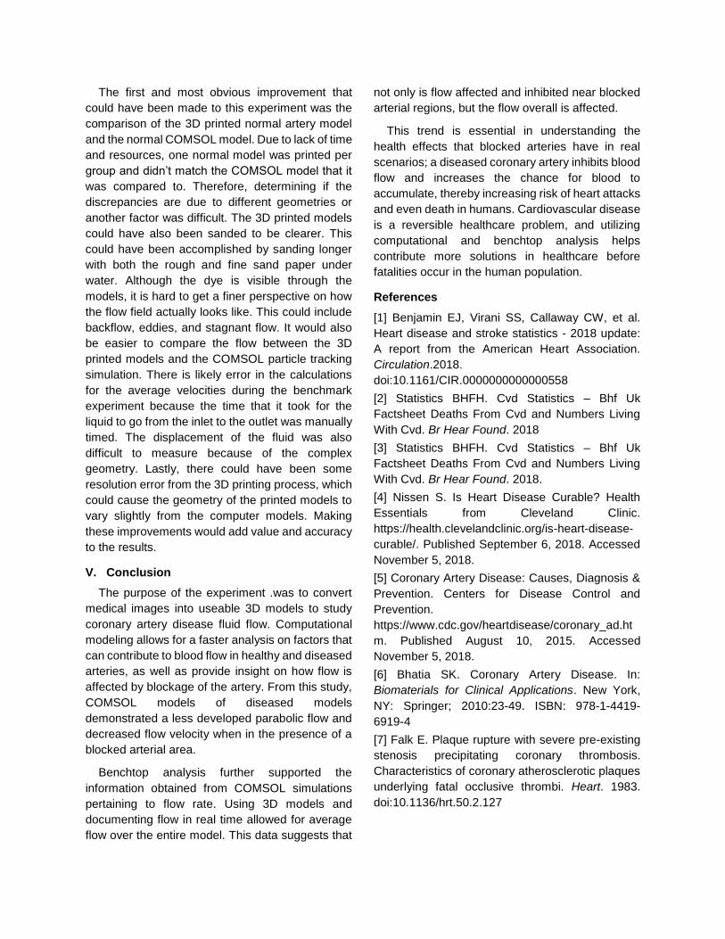
The first and most obvious improvement that

could have been made to this experiment was the

comparison of the 3D printed normal artery model

and the normal COMSOL model. Due to lack of time

and resources, one normal model was printed per

group and didn’t match the COMSOL model that it

was compared to. Therefore, determining if the

discrepancies are due to different geometries or

another factor was difficult. The 3D printed models

could have also been sanded to be clearer. This

could have been accomplished by sanding longer

with both the rough and fine sand paper under

water. Although the dye is visible through the

models, it is hard to get a finer perspective on how

the flow field actually looks like. This could include

backflow, eddies, and stagnant flow. It would also

be easier to compare the flow between the 3D

printed models and the COMSOL particle tracking

simulation. There is likely error in the calculations

for the average velocities during the benchmark

experiment because the time that it took for the

liquid to go from the inlet to the outlet was manually

timed. The displacement of the fluid was also

difficult to measure because of the complex

geometry. Lastly, there could have been some

resolution error from the 3D printing process, which

could cause the geometry of the printed models to

vary slightly from the computer models. Making

these improvements would add value and accuracy

to the results.

V. Conclusion

The purpose of the experiment .was to convert

medical images into useable 3D models to study

coronary artery disease fluid flow. Computational

modeling allows for a faster analysis on factors that

can contribute to blood flow in healthy and diseased

arteries, as well as provide insight on how flow is

affected by blockage of the artery. From this study,

COMSOL models of diseased models

demonstrated a less developed parabolic flow and

decreased flow velocity when in the presence of a

blocked arterial area.

Benchtop analysis further supported the

information obtained from COMSOL simulations

pertaining to flow rate. Using 3D models and

documenting flow in real time allowed for average

flow over the entire model. This data suggests that

not only is flow affected and inhibited near blocked

arterial regions, but the flow overall is affected.

This trend is essential in understanding the

health effects that blocked arteries have in real

scenarios; a diseased coronary artery inhibits blood

flow and increases the chance for blood to

accumulate, thereby increasing risk of heart attacks

and even death in humans. Cardiovascular disease

is a reversible healthcare problem, and utilizing

computational and benchtop analysis helps

contribute more solutions in healthcare before

fatalities occur in the human population.

References

[1] Benjamin EJ, Virani SS, Callaway CW, et al.

Heart disease and stroke statistics - 2018 update:

A report from the American Heart Association.

Circulation.2018.

doi:10.1161/CIR.0000000000000558

[2] Statistics BHFH. Cvd Statistics – Bhf Uk

Factsheet Deaths From Cvd and Numbers Living

With Cvd. Br Hear Found. 2018

[3] Statistics BHFH. Cvd Statistics – Bhf Uk

Factsheet Deaths From Cvd and Numbers Living

With Cvd. Br Hear Found. 2018.

[4] Nissen S. Is Heart Disease Curable? Health

Essentials from Cleveland Clinic.

https://health.clevelandclinic.org/is-heart-disease-

curable/. Published September 6, 2018. Accessed

November 5, 2018.

[5] Coronary Artery Disease: Causes, Diagnosis &

Prevention. Centers for Disease Control and

Prevention.

https://www.cdc.gov/heartdisease/coronary_ad.ht

m. Published August 10, 2015. Accessed

November 5, 2018.

[6] Bhatia SK. Coronary Artery Disease. In:

Biomaterials for Clinical Applications. New York,

NY: Springer; 2010:23-49. ISBN: 978-1-4419-

6919-4

[7] Falk E. Plaque rupture with severe pre-existing

stenosis precipitating coronary thrombosis.

Characteristics of coronary atherosclerotic plaques

underlying fatal occlusive thrombi. Heart. 1983.

doi:10.1136/hrt.50.2.127

[8] Izzo JL, Weir MR. Angiotensin-converting

enzyme inhibitors. J Clin Hypertens. 2011.

doi:10.1111/j.1751-7176.2011.00508.x

[9] Coronary Artery Bypass Grafting. National Heart

Lung and Blood Institute.

https://www.nhlbi.nih.gov/health-topics/coronary-

artery-bypass-grafting. Accessed November 5,

2018.

[10] Coronary angioplasty and stents. Mayo Clinic.

https://www.mayoclinic.org/tests-

procedures/coronary-angioplasty/about/pac-

20384761. Published December 30, 2017.

Accessed November 5, 2018

[11] Pop GA, Duncker DJ, Gardien M, et al. The

clinical significance of whole blood viscosity in

(cardio)vascular medicine. Neth Heart J.

2002;10(12):512-516.

[12] Calculate density and viscosity of

glycerol/water mixtures. Calculate density and

viscosity of glycerol/water mixtures.

http://www.met.reading.ac.uk/~sws04cdw/viscosity

_calc.html. Published April 4, 2018. Accessed

November 4, 2018.

A1. COMSOL Setup (Ted)

Table 2. Setting Up Laminar Flow Study

Define Space Dimension

Select Physics

Choose Laminar Flow

Select Study

Choose Time Dependent Study

Import Mesh

Right click on Mesh, select import, Change source to COMSOL Multiphysic file and import either the diseased or healthy model.

Create Material

Right click on Materials, select Blank Material.

Define Material

Select the Blank Material. Under Material Properties Select Density and Dynamic Velocity.

Define the Material properties Values under material content. Note the dynamic viscosity and density is equivalent to literature values of normal blood.

Define Fluid Properties

Under Fluid Properties, select the density to be from the material and the dynamic viscosity to be from the material.

Define Initial Values

Under the Initial Values set the pressure to be 11600 Pa which is equivalent to blood pressure in the coronary artery.

Define Wall Condition

Under Wall 1, select all surfaces except the inlet and outlet. Under the boundary condition tab change the wall condition from No Slip to Slip Velocity.

Define Inlet Conditions

Under Inlet 1, select the inlet surface of the model. Under Boundary Condition change it from Velocity to Laminar Flow. Select the Average velocity button. Define Average Velocity to be 0.233 m/s and entrance length to 0.2m to verify laminar flow. The average velocity value was determined from coronary artery research paper.

Define Outlet Conditions

Under Outlet 1, first select the outlet surfaces of the model. Under Boundary condition select Pressure. Under Pressure Conditions define the pressure to 11600 Pa and select the suppress backflow button.

Solve and Compute

The study settings can be selected as shown below. Once selected hit compute.

Results

Under Results the velocity field can be seen. To adjust the amount and location of slices the slice 1 settings can be Adjusted.

Table 3. COMSOL Particle Tracing Setup

Add Particle Tracking Physic to the Laminar Flow study.

Under the Home tab select Add Physics. Then Choose the Particle Tracing for Fluid Flow (fpt)

Add Study

Under the Home tab select Add Study. Then choose time dependent study.

Define Wall Conditions for Particle Tracing.

Under Wall 1, select the wall condition to Freeze.

Define Particle Properties for Particle Tracing.

Under Particle Properties 1, specify the particle properties to the values shown below.

Define the Inlet Conditions for Particle Tracing

Under Inlet 1, select the initial position and initial velocity settings shown below. Make sure the inlet surface is selected.

Define Outlet conditions for Particle Tracing

Under Outlet 1, make sure to select the outlet surface. Define the outlet wall condition to freeze.

Define Drag Force conditions for Particle Tracing

Under Drag force, in the drag force tab, make the selections below.

Define Study 2 Time dependent solver configurations.

Adjust the Values of dependent variables as seen below then hit compute. A Direct Solver should be used for computation. Make sure the first study has been computed, or the second study will not compute.

Results

Under Particle Trajectories the various time points of the particles and their velocities can be plotted. All the time points can be exported to a video by hitting the animation button, located in the particle trajectories tab.

A2. COMSOL Setup (Alex)

Table 4. Alex’s Comsol Table Including Laminar and Particle Tracing Physics Study:

Define the space

dimension

Start COMSOL Multiphysics. Model wizard>Select Space Dimension>2-D

axisymmetric>click on “next” arrow

Define the physics There are two physics studies performed in this module:

1. Time-Dependent Laminar Flow

2. Time -Dependent Particle Tracing for Fluid Flow

Define the study type Both physics studies are time-dependent.

Define the geometry The geometry was obtained by extracting a healthy and diseased

coronary artery using Mimics.

Define the material

type

The material of the fluid was blood. The density and dynamic viscosity

were 1060 kg/m^3 and 0.0032 Pa*s, respectively.

Physical Settings, initial

conditions

Laminar Flow Study

● The inlet pressure = 9,332.57 Pa (pressure of the blood inside the

coronary artery)

● outlet pressure = 9,332.57 Pa (pressure of the blood inside the

coronary artery)

● Inlet velocity = 0.029 m/s

Particle Tracing

● Drag law = stokes

● Inlet = 3000 particles released

Physical Settings

Boundary Conditions

● Wall condition for laminar flow study - no slip

● Wall condition for particle tracing - freeze

● Particle density = 2200 [Kg/m^3]

● Particle diameter = 5E-7 [m]

Mesh The mesh was created using 3 Matics program. The geometry of the

elements are triangles that were adjusted to make a finer mesh to get

more accurate result in the physics studies.

Study: Solve ● Laminar Flow Study - solving for velocities throughout model as a

function of time

● Particle Tracing - solving for particle displacements and velocities

throughout model as a function of time. This study uses results from

the laminar flow study.

Compute Click study 1 --

A3. COMSOL Setup (Sarea)

Table 5. Table Including Laminar and Particle Tracing Physics Study:

Define the space

dimension

Start COMSOL Multiphysics. Model wizard>Select Space

Dimension>2-D axisymmetric>click on “next” arrow

Define the physics

Fluid flow → Single-Phase Flow → Laminar Flow (spf)

Define the study type

Preset studies → Time Dependent

Define the geometry N/A - models were imported through the mesh

Define the material

type

Materials → Right-click Materials → select Blank Materials

→ select “Density”,”Dynamic Viscosity” under Materials

Content section

Physical Settings,

initial conditions

Fluid flow simulation:

Initial values: Pressure = 11600 Pa

Particle-tracking simulation:

Physical Settings

Boundary Conditions

Fluid flow simulation:

Fluid properties: dynamic viscosity = 3.2E-3 Pa*s density =

1060 kg/m3

Wall condition: no slip

Normal inflow velocity: Vo = 0.029 m/s

Outlet: P0 = 11600 Pa with suppressed backflow

Particle-tracking simulation:

Mesh

Mesh 1 → Import 1

Performed for healthy and diseased models

Study: Solve Fluid flow simulation:

Study 1 → Study 1: Time Dependent

Particle flow simulation

Study 2 → Study 2: Time Dependent → de-select “Solve

for” check for Laminar flow under the Physics and Variable

Selection subsection

Compute

Fluid flow simulation:

Study 1 → Solver Configurations → Solution 1 → Time-

Dependent Solver 1 → study type should be “Direct 1”

Particle flow simulation:

Study 2 → Solver Configurations → Solution 2 → Time-

Dependent Solver 1 → study type will be “Iterative 1”

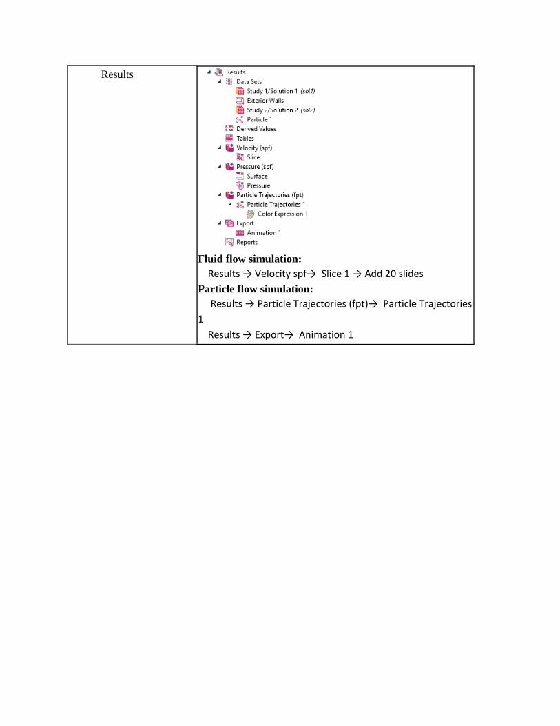
Results

Fluid flow simulation:

Results → Velocity spf→ Slice 1 → Add 20 slides

Particle flow simulation:

Results → Particle Trajectories (fpt)→ Particle Trajectories

1

Results → Export→ Animation 1