modeling and signal processing of low-finesse fabry-perot
TRANSCRIPT
Modeling and Signal Processing of Low-Finesse Fabry-Perot Interferometric Fiber Optic Sensors
Cheng Ma
Dissertation submitted to the faculty of the Virginia Polytechnic Institute and State University
in partial fulfillment of the requirements for the degree of
Doctor of Philosophy in
Electrical Engineering
Anbo Wang, Chair
Yong Xu
Ting-Chung Poon
Gary R. Pickrell
James R. Heflin
September 4, 2012 Blacksburg, Virginia
Keywords: Fiber Optics, Fiber Optic Sensors, Fabry-Perot, White-Light Interferometry
Copyright 2012, Cheng Ma
Modeling and Signal Processing of Low-Finesse Fabry-Perot Interferometric Fiber Optic Sensors
Cheng Ma
ABSTRACT
This dissertation addresses several theoretical issues in low-finesse fiber optic Fabry-
Perot Interferometric (FPI) sensors. The work is divided into two levels: modeling of the
sensors, and signal processing based on White-Light-Interferometry (WLI).
In the first chapter, the technical background of the low-finesse FPI sensor is briefly
reviewed and the problems to be solved are highlighted.
A model for low finesse Extrinsic FPI (EFPI) is developed in Chapter 2. The theory is
experimentally proven using both single-mode and multimode fiber based EFPIs. The
fringe visibility and the additional phase in the spectrum are found to be strongly
influenced by the optical path difference (OPD), the output spatial power distribution and
the working wavelength; however they are not directly related to the light coherence.
In Chapter 3, the Single-Multi-Single-mode Intrinsic FPI (SMS-IFPI) is theoretically and
experimentally studied. Reflectivity, cavity refocusing, and the additional phase in the
sensor spectrum are modeled. The multiplexing capacity of the sensor is dramatically
increased by promoting light refocusing. Similar to EFPIs, wave-front distortion
generates an additional phase in the interference spectrogram. The resultant non-constant
phase plays an important role in causing abrupt jumps in the demodulated OPD.
WLI-based signal processing of the low-finesse FP sensor is studied in Chapter 4. The
lower bounds of the OPD estimation are calculated, the bounds are applied to evaluate
OPD demodulation algorithms. Two types of algorithms (TYPE I & II) are studied and
compared. The TYPE I estimations suffice if the requirement for resolution is relatively
low. TYPE II estimation has dramatically reduced error, however, at the expense of
potential demodulation jumps. If the additional phase is reliably dependent on OPD, it
can be calibrated to minimize the occurrence of such jumps.
In Chapter 5, the work is summarized and suggestions for future studies are given.

iii
To Yanna
for the amazing support you have always provided

iv
Acknowledgements
I am indebted and thankful to my advisor, Dr. Anbo Wang, for providing me this opportunity to work on something I truly enjoy. I learnt so much from him in every aspects of my professional life. His encouragements gave me the courage to overcome difficulties, and gained me the confidence to develop an academic career. He is not only a wonderful advisor, but also a role model and a close friend.
I would like to thank the other committee members, Dr. Gary R. Pickrell, Dr. Yong Xu, Dr. Ting-Chung Poon, and Dr. James R. Heflin for their assistances throughout my research. I am deeply grateful to Ms. Mary L. Hallauer and Dr. William L. Hallauer for their tremendous help as teachers and friends.
I would like to thank my dearest friends and colleagues at CPT, Dorothy Wang, Kathy Wang, and Bo Dong for their help and friendship in the past 6 years. Thanks also extend to Dr. Evan Lally, Dr. Zhengying Li, Dr. Brian Scott, Dr. James Gong, Dr. Ming Han, Dr. Yizheng Zhu, Dr. Kristie Cooper, Dr. Baigang Zhang, Dr. Zhengyu Huang, Dr. Juncheng Xu, Dr. Fabin Shen and Ms. Debbie Collins for their helps, advices, and all kinds of contributions to my research..
Special gratitude goes to my best friends and teachers in Blacksburg—Bin Zhang & Juan Wang, Liguo Kong & Hong Tang, Chunlin Luo & Chen Tang & Bright Zheng, Teresa Ehrlich & David Ehrlich—for all the helps and beautiful memories they have brought.
I would like to express my deepest gratitude to my parents, who have been encouraging and supporting me to get this far. I would like to thank my wife, Yanna, for her persistent assistance and encouragement. Without her care and love, this dissertation would not have been possible.

v
Contents
Chapter 1 Introduction..................................................................................................... 1
1.1. Background .......................................................................................................... 1
1.1.1 Fiber-optic sensing in general ....................................................................... 1
1.1.2 Low-finesse fiber-optic Fabry-Perot interferometers ................................... 2
1.2. Signal processing approaches for low-finesse FO FPI ......................................... 2
1.3. Identification of problems .................................................................................... 3
1.3.1 Basic signal processing concept .................................................................... 3
1.3.2 Available methods for direct OPD estimation .............................................. 4
1.3.3 Brief review of WLI-FP signal demodulation algorithms ............................ 5
1.3.4 Brief review of low-finesse FO FP model .................................................... 7
1.3.5 Identification of problems ............................................................................. 8
Level 1: Physical modeling ..................................................................................... 8
Level 2: Signal processing ...................................................................................... 8
Chapter 2 Modeling of Fiber Optic Low-Finesse EFPI Sensors .................................. 9
2.1 Introduction .......................................................................................................... 9
2.2 Development of the theory ................................................................................. 10
2.2.1 Fundamental concepts ................................................................................. 10
2.2.2 The EFPI spectrum ..................................................................................... 12
2.2.3 Calculation of I(kz) ...................................................................................... 18
I(kz) calculation for SMF-EFPI ............................................................................. 18
I(kz) calculation for MMF-EFPI ........................................................................... 18
2.2.4 Wafer-based EFPI ....................................................................................... 20
2.3 Results and discussion ........................................................................................ 21
2.3.1 Air-gap SMF-EFPI: simulation and experimental results .......................... 21
2.3.2 Air-gap MMF-EFPI: comparison with previous literatures ........................ 25

vi
2.3.3 Air-gap MMF-EFPI: simulation and experimental results ......................... 28
2.3.4 Relationship with degree of coherence ....................................................... 31
2.3.5 Results for wafer-based EFPI ..................................................................... 32
Silica MMF excitation .......................................................................................... 33
Sapphire fiber excitation ....................................................................................... 33
2.3.6 Influence on WLI-based signal processing ................................................. 35
Air-gap EFPI ......................................................................................................... 35
Wafer-based EFPI ................................................................................................. 35
2.4 Conclusion .......................................................................................................... 37
Chapter 3 Modeling of Fiber Optic Low-Finesse IFPI Sensors ................................. 38
3.1 Introduction ........................................................................................................ 38
3.2 Basic models for sensor reflection and transmission ......................................... 39
3.2.1 Reflectivity of the cavity mirrors ................................................................ 39
3.2.2 GI-MMF cavity refocusing ......................................................................... 42
3.2.3 Verification of the refocusing model .......................................................... 50
Insertion loss reduction by cavity refocusing ....................................................... 50
Increasing the multiplexing capacity .................................................................... 52
3.3 Analysis of the IFPI additional phase ................................................................ 53
3.3.1 Modal analysis of the SMS-IFPI ................................................................. 54
Exact field expression ........................................................................................... 54
Two-mode excitation ............................................................................................ 55
Rotating vector picture .......................................................................................... 57
3.3.2 Further discussion of the additional phase .................................................. 61
Physical meaning of the OPD dependant phase term ........................................... 64
3.3.3 Verification of the additional phase ............................................................ 71
3.4 Signal processing of IFPI sensors ...................................................................... 75
3.4.1 Initial phase jump experiment ..................................................................... 76
3.4.2 Analysis of demodulation jumps ................................................................ 78
Non-constant phase-induced OPD demodulation jumps ...................................... 78
Origins of the non-constant phase term ................................................................ 81
3.4.3 Total phase interrogation method ............................................................... 84
3.4.4 Algorithm testing and results ...................................................................... 85

vii
Simulation of multimode-induced phase variation ............................................... 85
Simulation of sampling rate-induced phase variation ........................................... 87
Simulated noise performance ................................................................................ 88
Experimental evaluation of algorithm .................................................................. 88
3.5 Conclusion .......................................................................................................... 90
Chapter 4 WLI-Based Signal Processing ...................................................................... 92
4.1 Introduction ........................................................................................................ 92
4.2 Theory ................................................................................................................ 95
4.2.1 Background ................................................................................................. 95
4.2.2 The theories ................................................................................................. 98
Cause of the jump (I): the constant φ0 assumption ............................................... 98
Total phase estimation with varying φ0 ................................................................ 98
The lower bounds .................................................................................................. 99
Cause of the jump (II): estimation noise of φ0 .................................................... 101
4.3 Discussion ........................................................................................................ 102
4.3.1 WLI algorithms ......................................................................................... 102
The periodogram (FFT method) ......................................................................... 102
Linear regression (LR method) and peak tracking (PT method) ........................ 103
4.3.2 Evaluation of the algorithms ..................................................................... 103
4.3.3 Comparison of the algorithms ................................................................... 105
Estimator bias...................................................................................................... 105
Comparison of the algorithms ............................................................................. 107
4.3.4 OPD-dependent additional phase .............................................................. 109
Phase front distortion .......................................................................................... 109
Material dispersion.............................................................................................. 110
Fixed-pattern noise (FPN) ................................................................................... 110
Finite sampling rate (FSR) .................................................................................. 112
4.3.5 More on total phase ................................................................................... 112
The noise reduction mechanism of TYPE II estimations ................................... 112
Characteristics of the estimated total phase ........................................................ 115
Reducing the probability of jump in TYPE II estimations ................................. 116
4.4 Conclusion ........................................................................................................ 118

viii
Chapter 5 Summary and Future Work ...................................................................... 120
5.1 Summary .......................................................................................................... 120
5.2 Contributions and publications ......................................................................... 122
5.3 Recommendation for future work .................................................................... 123
5.3.1 Elimination of the demodulation jumps .................................................... 123
5.3.2 Improvement of the fringe visibility ......................................................... 124
5.3.3 Development of universal FPI demodulation software ............................ 124
5.3.4 Application of the FV-I(kz) relationship ................................................... 125
Bibliography .................................................................................................................. 126

ix
List of Figures
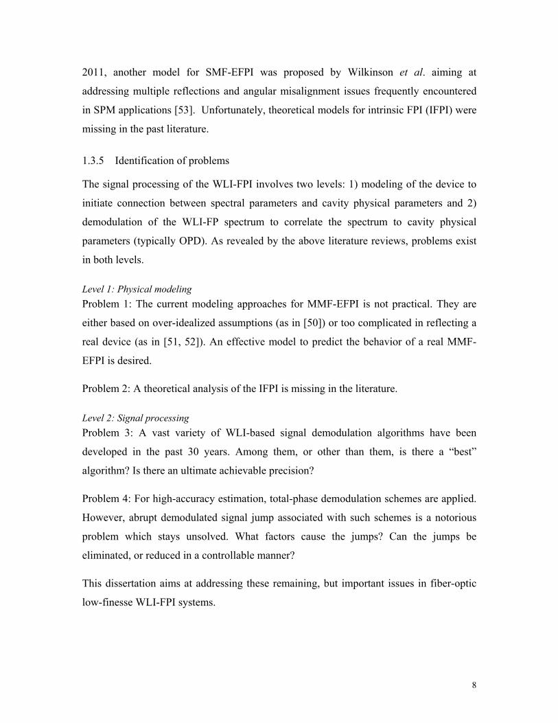
Figure 2.1. EFPI sensor schematics and spectrum. (a) EFPI sensor with air-gap cavity. (b)
EFPI sensor with wafer cavity. (c) a typical sensor spectrum. ...................... 11
Figure 2.2. Schematic of the optical fiber low-finesse EFPI. ........................................... 12
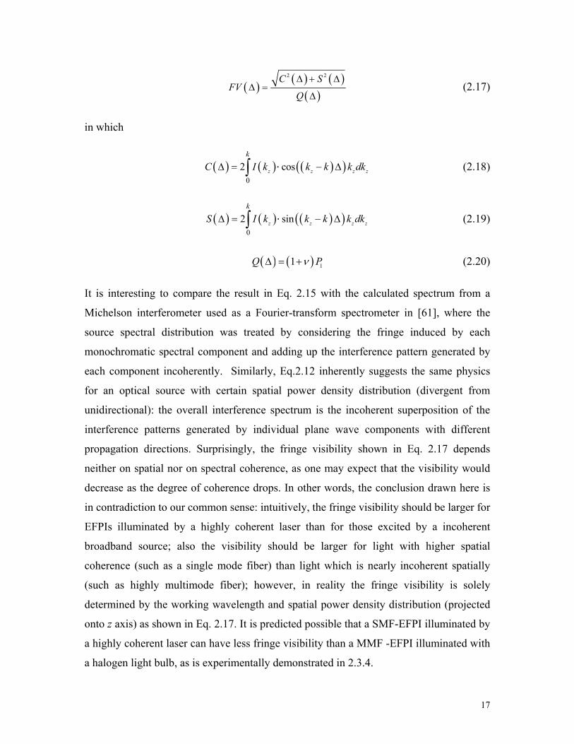
Figure 2.3. Conversion schematic from angular power density distribution to the kz
density distribution. The total power distributed from kz to kz+dkz is equal to
the power flux in the ring area (in green color) defined by divergence angle
from θ to θ + dθ. ............................................................................................ 19
Figure 2.4. Experimental setup for measurement of the fringe visibility curve. Parallelism
of the two reflection surfaces are guaranteed by tuning the two rotation stages,
and the cavity length can be finely tuned by a 1-D translation stage. ........... 22
Figure 2.5. Fringe visibility plotted as a function of FP cavity length. Solid and dashed
curves represent simulation results, circles and dots are experimental data.
The calculated mode field radii of the fibers are labeled and compared with
the values in their specifications. ................................................................... 23
Figure 2.6. Conceptual illustration of the relationship between output divergence angle
and the visibility curve. (a) I(kz) distribution of a beam with less divergence
angle. (b) Visibility curve corresponding to the distribution in (a). (c) I(kz)
distribution of a beam with larger divergence angle. (d) Visibility curve
corresponding to the distribution in (c). The figures show qualitatively that
the visibility curve gets broader as I(kz) becomes sharper. ............................ 23
Figure 2.7. Theoretical and experimental data showing the extra phase delay of an EFPI
with SMF-28 as the lead-in fiber. .................................................................. 25
Figure 2.8. Fringe visibility versus FP cavity length for fiber 1,2 and 3, all modes are
equally excited.. ............................................................................................. 28
Figure 2.9. Theoretical and experimental results of the fringe visibilities and additional
phases versus OPD for MMF-EFPI. MMF has core diameter 105μm and
NA=0.22. (a) Measured angular distribution. (b) Calculated I(kz) distribution
based on (a). (c) Fringe visibility versus OPD curve for 800nm, 1200nm and

x
1550nm light, theoretical and experimental. (d) Additional phase θ versus
OPD for 800nm, 1200nm and 1550nm light, theoretical. ............................. 29
Figure 2.10. Comparing the fringe visibility curves of two EFPIs. Due to its smaller
output divergence angle, an MMF-EFPI illuminated by halogen lamp shows
better fringe visibility than a SMF-EFPI illuminated by a highly-coherent
laser. ............................................................................................................... 31
Figure 2.11. Visibility curve calculation: (a) Measured beam angular distribution from a
0.22 NA silica fiber. (b) Calculated fringe visibility for both air-gap and
wafer FP cavities based on the characterized angular distribution. ............... 33
Figure 2.12. Visibility curve calculation: (a) Comparison of measured beam angular
distribution from a sapphire fiber and a 0.22 NA silica fiber. (b) Fringe
visibilities of a sapphire wafer EFPI with sapphire fiber and 0.22 NA silica
fiber excitations, calculated based on the characterized angular distribution in
(a). .................................................................................................................. 34
Figure 2.13. Additional phase as a function of OPD for EFPI cavities. (a) Experimental
and theoretical additional phases captured as a function of OPD for an air-gap
EFPI. (b) Experimental and theoretical additional phases of a wafer-based
EFPI show strong OPD-dependence as a result of material dispersion. ........ 36
Figure 3.1. Schematic of the SMS-IFPI sensor. ............................................................... 38
Figure 3.2. Computation procedure to calculate m(z) for the index profile shown in (a).
The m profile, shown in (b), can be decomposed as a convolution of the
functions shown in (c) and (d). ...................................................................... 41
Figure 3.3. Relative reflectivity as a function of index profile transition width. Solid,
dashed and dot-dash curves represent 1550, 800 and 2300 nm, respectively.
....................................................................................................................... 42
Figure 3.4. Five lowest order mode profiles of MMF1. The fundamental mode profile of
the excitation SMF is also plotted for comparison. All the modes are
normalized, and SMF and MMF core boundaries are marked. ..................... 47
Figure 3.5. Light propagation in multimode fibers. (a) Field amplitude distribution in GI-
MMF (MMF2). (b) Field amplitude distribution in SI-MMF, whose
parameters are identical to MMF2. ................................................................ 48
xi
Figure 3.6. Calculated and experimental results for the coupling loss and beam radius of
the GI-MMF. (a) Coupling loss variation as MMF length and (b) Beam radius
variation as MMF length. For the simulation, the MMF1 fiber is selected.
Corning InfiniCor600 was used for the experiment. ..................................... 50
Figure 3.7. Experimental results showing the benefit of IFPI cavity length control. In (a),
the FFT of the spectra for a link with (solid) and without (dashed) refocusing
are compared. The relative OPD estimation error for each sensor in the links
is plotted in (b). .............................................................................................. 52
Figure 3.8. Design of a sensing link with 22 IFPI sensors multiplexed with three different
types of MMF. 62.5/125 MMF: Thorlab GIF-625; 50/125 MMF: Corning
InfiniCor600; 100/140 MMF: OFS-100/140. ................................................ 53
Figure 3.9. Additional phase term for a two-mode cavity at different excitation ratios. .. 57
Figure 3.10. Relationship between the total field vector and five individual mode vectors.
....................................................................................................................... 58
Figure 3.11. Zoom-in view of the rotating vectors. Nine groups of vectors are plotted
with equal angular spacing such that υ1 rotates exactly 2π. Dark lines: first
group of vectors (beginning position); gray lines: last group of vectors (end
position: υ1 coincides with υ1 in the first group, υ2 is a little behind υ2 in the
first group; the effective vector Σ is ahead of Σ in the first group). Inset:
global view of the vector rotation. Upper-left arrow: position of the first and
last groups of vectors; other arrows illustrate the rotational direction of the
vectors. ........................................................................................................... 59
Figure 3.12. Relative phase shift to LP01 mode as k increases. Plotted are phase shifts of
LP02 mode, the effective vector Σ, and a virtual mode with neff=nestimate. ...... 60
Figure 3.13. Spectral phase shift induced by OPD estimation error ................................. 62
Figure 3.14. Simulated linear fitting error as a function of wavenumber. ........................ 65
Figure 3.15. Computer simulated relative phase change as cavity length increases. ....... 66
Figure 3.16. Estimated neff as the cavity length increases while all the refractive indices
stay unchanged. Two horizontal lines mark the refractive indices of the MMF
core and cladding. .......................................................................................... 67
Figure 3.17. Graphical explanation of the additional phase term ..................................... 68

xii
Figure 3.18. Phase difference as a function of cavity length ............................................ 70
Figure 3.19. Phase difference as a function of temperature, measured by direct
comparison of the predicted spectrum and the real spectrum. Inset: measured
by using Eqs.3.48 and 3.49. ........................................................................... 70
Figure 3.20. The evolution of the additional phase term θ with cavity length L. (a) The
additional phase term in GI-MMF (MMF2). (b) The additional phase term in
SI-MMF, whose parameters are identical to MMF2. .................................... 73
Figure 3.21. Verification of the analysis of the additional phase term θ in (26). The
experimental demonstration is achieved by comparing the estimation of δn by
two approaches for ten sensors multiplexed in a link. ................................... 73
Figure 3.22. Additional phase term as a function of OPD. ............................................... 75
Figure 3.23. Output of a high-quality SMS-IFPI sensor under smoothly increasing
temperature. When interrogated using traditional OPD techniques, the sensor
experiences an abrupt jump in its demodulated signal. ................................. 77
Figure 3.24. (a) Slope κ of the OPDm(1) vs. m curve as a function of phase estimation
error Δ (b) An example of the tilting at a phase shift Δφ ≈ π, given by the
OPDm(1) vs. m curves for n(1) = 27 and n(1 )= 28............................................. 80
Figure 3.25. OPD of an IFPI sensor (demodulated using traditional constant phase and
new total phase algorithms) and its phase shift Δφ under increasing
temperature. Spectral data generated by computer simulation ...................... 86
Figure 3.26. Comparison of simulated, experimental and theoretical variations in initial
phase φ0(τ) due to finite wavelength scan rate S. .......................................... 87
Figure 3.27. Performance of the varying total phase algorithm evaluated at different
cavity lengths and SNR levels. MSE errors were calculated based on 1000
sampling points, among which phase shift from 0- 1.2π was evenly
distributed. Each spectrum contains 20000 points spaced over 1520-1570nm.
....................................................................................................................... 88
Figure 3.28. IFPI sensor OPD (demodulated using traditional constant phase and new
total phase algorithms) and total phase Φ=k·OPD+φ0 during an experimental
controlled temperature increase. .................................................................... 89
xiii
Figure 3.29.IFPI strain sensor evaluation: demodulated by (a) traditional fixed-phase
OPD method, (b) new varying total phase method ........................................ 89
Figure 4.1. Schematic of the fiber optic WLI -FP sensing system. .................................. 93
Figure 4.2. Performance evaluation of the FFT, LR and PT methods, plotted together in
both figures are the standard deviation of both the TYPE I and TYPE II
estimators. a: OPD estimation and b: φ0 estimation. The CRBs for the
corresponding variances are co-plotted. Insets are zoomed-in views of the
curves, which provide better visibility of the algorithms’ performances. ... 104
Figure 4.3. Absolute value of OPD bias versus cavity length plotted for TYPE I LR, FFT
and windowed FFT (Blackmanharris) estimators. The result for TYPE II
estimator using FFT (Blackmanharris) is co-plotted, which demonstrates
superior bias suppression. ............................................................................ 106
Figure 4.4. Performance comparison of the LR, FFT and windowed FFT
(Blackmanharris). The RMS error includes the contributions from both the
estimator variance and bias. The windowed FFT for both TYPE I and TYPE
II estimations manifests superior performance in bias reduction, at the
expense of a ~3dB increase in the RMS error. ............................................ 108
Figure 4.5. Measured computation complexity in terms of execution time, plotted as a
function of data length (N). The FFT, PT and LR methods are compared to
demonstrate linear relationship with N. The complexity of FFT is the highest
while the complexities of PT and LR are almost identical. ......................... 109
Figure 4.6. Computer-simulated phase term φ0 caused by material dispersion (solid) and
fixed-pattern noise (dashed). The dispersion of a 70μm-thick silica wafer was
modeled by the temperature-dependent Sellmeier model. WLI System I,
together with Blackmanharris windowed FFT was used for signal
demodulation. For the simulation of fixed-pattern noise, the applied white
Gaussian noise yields a SNR = 12 dB. ........................................................ 111
Figure 4.7. Computer-simulated variance and covariance terms in Eq. 4.29. The
corresponding CRBs are plotted together. An important observation is that
the variance terms and the covariance term cancel to yield a significantly
reduced variance for the total phase estimation. .......................................... 114

xiv
Figure 4.8. Experimentally obtained PDF of φ0 estimation. ........................................... 116
Figure 4.9. Reduction of jump probability by phase calibration. a: PDF of φ0 estimation
plotted with OPD, σp = 0.158π. The area between the solid lines is the
assigned phase range assuming constant phase, dashed lines are the
boundaries of the OPD-calibrated range with linear fitting. b: The
corresponding probability of jump. Solid line: OPD-dependent jump
probability for the constant range scheme. Dashed line: jump probability for
the calibrated range scheme. ........................................................................ 117

xv
List of Tables
Table 2.1. MMF Parameters. ............................................................................................ 27
Table 3.1. Splicing parameters for SMS-IFPI sensors. ..................................................... 42
Table 3.2. Fiber parameters used for the simulation. ........................................................ 46
Table 3.3. Power coupling coefficients of five MMF modes ........................................... 46
Table 3.4. Key properties of three types of MMF. ........................................................... 53
Table 3.5. Key variables used in the analysis. .................................................................. 77
Table 3.6. Simulation parameters for SMS-IFPI sensor. .................................................. 86
Table 4.1. List of key parameters of the WLI systems used in the research. ................... 98

1
Chapter 1 Introduction
1.1. Background
1.1.1 Fiber-optic sensing in general
The development of optical fibers is a scientific and technological miracle, the
significance of which has been recognized by the 2009 Nobel Prize. Besides their glaring
triumph in telecommunication, optical fibers have brought the industrial world another
revolution in the area of sensing. Made from purely insulating dielectric materials
(typically fused silica), fibers show significant improvements in their immunity to
electromagnetic interference (EMI) and corrosion; as such, when sensors are made using
the fibers, they fit perfectly to sensing applications where EMI and/or corrosion are of
major concerns. The extremely low transmission loss and high melting temperature also
benefit applications requiring long-distance, harsh-environment measurements. Being
developed for nearly three decades, fiber-optic (FO) sensing has achieved wide
commercialization [1, 2], and the technology is still expanding vigorously [3-5].
Two effects in the fiber have been widely explored as major sensing mechanisms. The
first effect is distributed linear or nonlinear scattering along the fiber. Such scatterings
(Rayleigh, Raman, Brillouin, etc.) can be generated along the whole fiber, their temporal
and spectral features can be affected by physical parameters such as temperature and
strain. Fully distributed FO sensing technologies (capable of measuring a one-
dimensional span from hundreds of meters up to tens of kilometers in a spatially
continuous manner) are mainly based on this mechanism [6-8]. The second effect
involves optical interference inside the fiber. Whenever the optical beam transmitted
inside the fiber is split into multiple parts (by locally distributed reflection or scattering),
they will interfere once re-coupled back to the original transmission mode. Devices
which can perform such beam-splitting and re-coupling can be generally classified as FO
interferometers, such as Mach-Zehnder (MZ), Fabry-Perot (FP), Michelson, Sagnac
interferometers, and fiber gratings [9, 10]. The split beams travel with different phase
velocities or through distinct optical paths (or both), and thus their interference produces
spectral patterns encoded with the optical path difference (OPD) among them. Because
the interference is sensitive to OPD change as small as a fraction of the optical

2
wavelength (sub-micrometer), such devices can be used as highly sensitive single-point
or multi-point (quasi-distributed) sensing elements. This project deals with signal
processing issues of one type of such devices, the low-finesse FO-FP interferometers.
1.1.2 Low-finesse fiber-optic Fabry-Perot interferometers
Low-finesse means that the two reflection surfaces forming the FP cavity have similar
but low reflectivities (typically less than 7% power reflectivity), so secondary reflections
do not contribute much to the spectral pattern of the interference spectrum. If one of the
surfaces (usually the one on the far-end from the lead-in beam) is coated with highly
reflective coating which generates a higher reflection, this structure is sometimes referred
to as a FO Fizeau interferometer [11]. Because secondary reflections inside a Fizeau
interferometer can also be neglected for most cases, it can be classified as low-finesse
and is accordingly covered by this research. The technical strategy behind “low-finesse”
is to minimize fabrication complexity (thus bring down the cost) and maximize sensor
robustness. The cost and structural/chemical instabilities (at high temperatures)
associated with highly-reflective coatings tend to jeopardize sensor performance and cost,
and is thus avoided universally in the sensing community.
In the past two decades, the Center for Photonics Technology at Virginia Tech involved
in developing all kinds of low-finesse FO FP sensors. Sensors have been developed to
measure temperature, strain, pressure, acoustic emission, EM fields, acceleration, partial
discharge, biological/chemical agents, etc.[12-16]. The success of the technology does
not only stay within the lab, but also extends to field applications. Our field tests clearly
demonstrated the technology’s superior capabilities over their electrical counterpart, and
help to secure a niche market for such devices.
1.2. Signal processing approaches for low-finesse FO FPI
One of the major achievements of the FO-FPI is its ability to perform high-precision
distance/ displacement measurements, which has been widely adopted in Scanning Probe
Microscopy (SPM) [17-19]. Such applications only involve displacement measurement of
much less than a wavelength, in which case quadrature detection may be well
approximated as linear, and displacement sensitivity as high as 2 fm/(Hz)1/2 was achieved

3
[20]. For measurements involving larger OPD change, single laser or dual-laser
arrangements were used in a “fringe counting” mode [21, 22]. Such narrow line-width
laser based technologies only provide relative OPD measurements, and suffer from
intensity noise. Multiplexing is also difficult to achieve using this method.
In many applications, absolute OPD measurement is essential. In such practices, white-
light interferometry (WLI) is widely adopted. The term “WLI” often refers to two
different technologies when applied to FO FPI. The first technology (denoted as type 1
WLI) utilizes a low-coherent broadband source together with another local OPD-
scanning interferometer to interrogate the sensor’s OPD by reading the maximum of the
total interference when the OPDs of the two interferometers match [23-26]. The second
technology (type 2 WLI) employs a spectrometer (either a broadband source with a
monochromater or a wavelength-swept laser with a detector) to interrogate the
interference spectrum of the FPI, which gives direct estimation of the OPD [27]. Both
methods have their own pros and cons. For the first technology, absolute measurement is
readily achieved, at the expense of higher system complexity. The second scheme
significantly simplifies the system and opens up possibility for multiplexing. However,
effective and reliable signal processing remains challenging, as will be detailed in the
next section. This project will focus on solving some key signal processing issues in the
type 2 WLI-FP systems.
1.3. Identification of problems
1.3.1 Basic signal processing concept
The interference spectrum of the low-finesse FPI can be written as
0 01 cosI FV k OPD (1.1)
where FV is a real number between 0 and 1, denoting the fringe visibility, which is
directly related to the signal to noise ratio (SNR). k0 is the wavenumber in vacuum,
defined by k0 = 2π/λ0, where λ0 is the wavelength in vacuum. OPD is the parameter to be
determined, it is related to the FP cavity parameter as OPD=2neffL, where neff is the
effective refractive index of the FP cavity medium, and L is the physical cavity length. φ0

4
is the initial phase (or additional phase) term, the significance of which has been
underestimated in the past. A detailed analysis and treatment of this phase term will be a
major task in this project. The total phase, or phase of the fringe, is defined through φtot =
k0OPD + φ0. The whole story of WLI based FP signal demodulation lies in estimating the
frequency (OPD) of a given sensor spectrum I. In general, the demodulation algorithms
fall within two categories.
Category 1: OPD estimation. This approach directly estimates the “frequency” of the
spectrum (OPD). It provides absolute measurement, but the accuracy is comparatively
low.
Category 2: Total phase estimation. Tracking the spectral position of a single point (or
multiple points), such as peaks and valleys, always yields much accurate characterization.
However, this method relies on the assumption that the particular fringe on which the
special observation point resides can be identified. When applied to spectrum with one
“fringe” being easily identified (such as fiber Bragg grating), this method works fine;
however it encounters tremendous difficulty when applied to FP demodulation, due to the
fact that all fringes appear to be identical. Noise and shift of the additional phase φ0 can
both result in misinterpretation of the fringe order, and this so-called phase ambiguity (or
2π ambiguity, fringe order ambiguity) will give rise to abrupt discontinuities (or simply
put, “jumps”) in the demodulated cavity length. In a word, higher estimation accuracy
always comes at the expense of non-absolute measurement, as reflected by the risks of
demodulation jumps.
1.3.2 Available methods for direct OPD estimation
Direct OPD estimation is of special importance due to two facts: 1) It offers absolute
measurement of the cavity length and 2) fringe order determination in high-resolution
peak-tracking approaches relies on accurate OPD estimation.
OPD estimation in Eq. 1.1 is in principle identical to frequency estimation of a discrete
time-domain signal, with the evenly sampled temporal points being substituted with
evenly sampled points in the wavenumber domain. Two classes of methods are typically
used for frequency estimation in sinusoidal signals: non-parametric frequency estimation

5
(classical) and parametric frequency estimation (modern). In classical frequency
estimation, typical approach involves computing the periodogram of the signal (by using
fast Fourier transform, FFT). For circumstances where periodogram fails to provide
satisfactory results (especially poor spectral resolution), parametric spectral estimation
methods are employed. Some of the most popular algorithms are: autoregressive-moving-
average (ARMA) model estimation, Pisarenko harmonic decomposition (PHD), multiple
signal classification (MUSIC), and estimating signal parameter via rotational invariance
techniques (ESPRIT), etc [28, 29]. To date, most signal processing approaches employed
for WLI -FP signal demodulation are based on non-parametric estimation. Only very few
papers report WLI-FP spectral characterization using parametric approaches [30].
1.3.3 Brief review of WLI-FP signal demodulation algorithms
In 1992, Chen et al. proposed a method to track the peak position of the fringe in the
spectrum [31]. This method is in principle a total phase approach; for applications
involving larger cavity length change (over λ/2), fringe ambiguity will come into play.
The basic idea has been developed over the years and was widely adopted as “peak
tracking” method [32, 33]. In the early 90’s, Claus et al. developed a simple method to
demodulate the cavity length of a fiber FP sensor [34]. Denoting two neighboring fringe
peaks (or valleys) in the spectrum as λ1 and λ2, cavity length can be readily obtained using
1 2 1 2/ 2 effd n (1.2)
This method is afterwards named the “peak-to-peak” method and sought wide
applications and developments [35, 36]. The approach is very simple and provides
absolute measurement, however, it is very sensitive to noise, as the noise term on the
denominators tends to be amplified. In the late 90’s, using the FFT peak to directly
indicate the cavity length was proposed and the accuracy of this approach was improved
by interpolation or zero-padding [37, 38]. This approach also provides absolute
measurement, but suffers from low accuracy, as the peak-to-peak method. In 2003, Qi et
al. developed an approach aiming to solve both the poor accuracy and fringe ambiguity
problem [39]. The method uses Eq. 1.2 to estimate the fringe order, and applies peak-
tracking to determine the cavity length. This approach is apparently an attempt to use

6
total phase demodulation, and solves the fringe ambiguity problem to some extent.
However, it has several constrains. First, the algorithm performs better when total
number of fringes in the spectrum is reduced. As fringe number increases, using only two
peaks to determine the fringe order and only one peak to calculate the cavity length loses
too much information. Secondly, fringe order ambiguity problem still exists. This is due
to two facts: 1) use Eq.1.2 to estimate the fringe order is still too noisy to provide reliable
predictions and 2) the method is based on the assumption that the additional phase term
in Eq. 1.1 is a constant. In 3.4.2, it will be shown that any algorithm with the assumption
of constant additional phase is intrinsically problematic and will lead to fringe order
ambiguity. In 2004, Han et al. proposed a method based on curve fitting to estimate the
cavity’s OPD [40]. The method recognized the non-constant additional phase term in Eq.
1.1, and accordingly treated this term by a theoretical model. This method is basically a
total phase approach and thus is susceptible to fringe ambiguity; meanwhile, it is only
applicable to single-mode fiber (SMF) based extrinsic FPI (EFPI, the definition of which
will be given in Section 2). In 2005, Shen et al. proposed a phase-linear-regression
method to perform the frequency estimation of the interference spectrum [27]. The
approach is divided into two parts. In the first step, a phase-linear-regression estimation is
carried out using the entire spectrum which gives comparatively low-quality OPD
estimation; in the second step, a correction is made to the first-step estimation based on
pre-stored information regarding the additional phase in Eq. 1.1. This approach shows
excellent precision, because it effectively uses the whole spectrum for estimation.
However, in order to have higher precision, total phase approach is applied in step two
with the assumption that the additional phase is a constant, which intrinsically will lead to
fringe order ambiguity and subsequently cause demodulation jumps. From the year 2006
to 2011, new algorithms were published each year, with incremental improvements to the
previous ones. For example, algorithms proposed by Jiang (2008) [41-43], Majumdar et
al. (2009) [44, 45] used direct OPD estimation methods (phase-linear-regression and FFT
for absolute measurement), and the work by Huang (2006) [46] and Zhou et al. (2011)
[47] reported methods based on curve fitting which fell in the category of total phase
demodulation. In 2006, Rao et al. published a FP signal demodulation algorithm using

7
Pisarenko harmonic decomposition (PHD), which is a parametric method giving direct
OPD estimation [30, 48].
1.3.4 Brief review of low-finesse FO FP model
Physical models describing the spectral behavior of low-finesse FP cavities are
indispensable in WLI-FP signal processing mainly due to 1) A good physical model helps
to interpret the FP spectrum, which leads to better estimation of the OPD and 2) An
effective model brings the sensor design to a higher engineering level to improve the
signal demodulation quality by improving the SNR and reducing the additional phase
shift.
In 1991, Murphy et al. modeled single-mode-fiber (SMF) extrinsic FPI (EFPI, in which
the light diffracts into free space inside the cavity) by regarding the fiber end face as a
point source and treated wave propagation using ray optics [22]. The model can roughly
explain fringe visibility drop at larger OPD but fails to account for additional phase φ0 as
shown in Eq. 1.1. In 1995, Arya et al. treated the SMF-EFPI problem numerically using
diffraction theory, and gave much better agreement between measured and predicted
fringe visibility as a function of OPD [49]. The drawbacks of the model were lack of
analytical expression and ignorance of the additional phase term. In 1999, Perennes et al.
published their work in modeling the multimode-fiber (MMF) EFPI by a geometrical
optics treatment [50]. The model only works for cases when “even excitation” condition
is fulfilled (all the modes in the MMF are equally excited); however, this assumption is
invalid for most applications. In 2004, Han et al. published a more rigorous model for
MMF-EFPI, in which fiber mode analysis was used to precisely describe the FP cavity
[51]. The model gave clear insights into the physics of the MMF-EFPI, and drew some
important conclusions. Later in 2006, the same authors announced the implication of the
model on an additional phase shift, which was surprisingly dependent on modal-
excitation condition in the MMF [52]. However, a drawback of the model is its
complexity and lack of analytical solution. For a standard MMF, mode excitation
condition in the MMF fiber is difficult to be analyzed exactly, upon which the model is
relied. In 2004, Han et al. reported an analytical model rigorously describing SMF-EFPI,
and the wave-propagation induced additional phase term was well interpreted [40]. In
8
2011, another model for SMF-EFPI was proposed by Wilkinson et al. aiming at
addressing multiple reflections and angular misalignment issues frequently encountered
in SPM applications [53]. Unfortunately, theoretical models for intrinsic FPI (IFPI) were
missing in the past literature.
1.3.5 Identification of problems
The signal processing of the WLI-FPI involves two levels: 1) modeling of the device to
initiate connection between spectral parameters and cavity physical parameters and 2)
demodulation of the WLI-FP spectrum to correlate the spectrum to cavity physical
parameters (typically OPD). As revealed by the above literature reviews, problems exist
in both levels.
Level 1: Physical modeling
Problem 1: The current modeling approaches for MMF-EFPI is not practical. They are
either based on over-idealized assumptions (as in [50]) or too complicated in reflecting a
real device (as in [51, 52]). An effective model to predict the behavior of a real MMF-
EFPI is desired.
Problem 2: A theoretical analysis of the IFPI is missing in the literature.
Level 2: Signal processing
Problem 3: A vast variety of WLI-based signal demodulation algorithms have been
developed in the past 30 years. Among them, or other than them, is there a “best”
algorithm? Is there an ultimate achievable precision?
Problem 4: For high-accuracy estimation, total-phase demodulation schemes are applied.
However, abrupt demodulated signal jump associated with such schemes is a notorious
problem which stays unsolved. What factors cause the jumps? Can the jumps be
eliminated, or reduced in a controllable manner?
This dissertation aims at addressing these remaining, but important issues in fiber-optic
low-finesse WLI-FPI systems.

9
Chapter 2 Modeling of Fiber Optic Low-Finesse EFPI Sensors
2.1 Introduction
The spectrum of fiber optic low-finesse extrinsic Fabry-Perot (FP) interferometers (EFPIs)
is studied in this chapter. Such fiber coupled interferometers have been demonstrated as
highly sensitive and robust sensors for measurement of temperature [14, 54], strain [11],
pressure [55, 56] and acoustic wave [57]. White-light interferometry [39], in which the
interferometer is illuminated either by a broadband optical source or a wavelength-
tunable laser and its reflected spectrum is analyzed, has shown promising advantages
over other interrogation counterparts in terms of demodulation accuracy, absolute
measurement and immunity to optical power instability. In order to make accurate and
reliable measurements, the sensor spectrum needs to be characterized carefully, some
advanced signal processing algorithms have been developed to this end [27, 39, 40].
While it is well understood that the demodulation error scales with noise power in the
spectrum [58], the demand for high fringe visibility becomes crucial, especially if a
multimode fiber (MMF) is used for excitation. During the past few years, it has been
reported in several publications [40, 59, 60] that the additional phase in the spectrum also
plays an important role in signal processing, which may potentially lead to abrupt jumps
in the demodulated sensor cavity length (see 3.4.2). As such, in-depth theoretical
modeling for both single-mode fiber (SMF) and MMF based EFPIs have been
investigated in the past two decades [40, 49-51], aiming to find the dependence of sensor
output spectrum on sensor geometry and optical property.
Arya et al. [49] addressed the fringe visibility of SMF-EFPI by considering diffraction in
the interferometer cavity, the similar approach was extended to study the beam
propagation (diffraction) and re-coupling induced additional phase term by Han et al.
[40]. While SMF-EFPI manifests well-defined electromagnetic (EM) field profile in the
cavity, MMF-EFPI does not: because MMF can have very diverse mode excitation
conditions, each guided mode has its individual mode profile yet the phase differences
among the excited modes are extremely complex, this poses considerable difficulties in
modeling the MMF-EFPI. Pérennès et al. [50] developed a simple geometrical-optics
approach, their theory led to an analytical solution for the fringe visibility, but was not

10
sufficiently accurate for many real applications. Han et al. [51, 52] treated the problem
with a more rigorous EM field approach using optical fiber mode theory, and both the
fringe visibility and additional phase issues have been addressed. All the above theories
contributed to our understanding of the EFPI fiber sensor behavior; however, several key
issues still remained unsolved.
The models based on rigorous EM field treatments, although promising in computing
good numerical solutions, encounter difficulties at bridging the physical model with real-
world applications, for example, mode excitation in MMF can be very complex, and may
vary upon multiple environmental factors; all these factors can couple together to make
the problem extremely complicated. In addition, several basic questions have yet been
satisfactorily answered. In experiments, it is found that the fringe visibilities of MMF-
EFPIs typically fade much faster as the cavity lengths increase than SMF-EFPIs do. How
does this phenomenon relate to the temporal and spatial degree of coherence of the output
light from the excitation fiber? In intrinsic Fabry-Perot interferometric (IFPI) sensors, the
cavity-length-dependent additional phase can ultimately lead to demodulation
discontinuities (see 3.4.2)[12]. Will this additional phase also behave similarly for the
EFPI sensors? In principle, any fiber can experience a smooth transition from single
mode-few mode-multimode operation without clear boundaries. Is there a unified theory
applicable to all these working conditions? The theory described in the following
subsection aims to solve these problems.
2.2 Development of the theory
2.2.1 Fundamental concepts
The subject is optical fiber low-finesse EFPIs. For the two types of dielectric materials
typically encountered in EFPIs—silica and sapphire, the power reflectivities are
approximately 4% and 7% respectively, sufficiently small to neglect multiple reflections
inside the FP cavity. The word “extrinsic” refers to free-space propagation of the optical
beam inside the cavity, as in contrast to “intrinsic”, in which case the propagation of the
beam is assumed to be guided.
11
Figure 2.1. EFPI sensor schematics and spectrum. (a) EFPI sensor with air-gap
cavity. (b) EFPI sensor with wafer cavity. (c) a typical sensor spectrum.
The free-space propagation of the light can either be in air or in dielectric. For the former,
the two reflections are formed by two polished optical fiber ends, and the two fibers are
aligned inside a capillary tube, as shown in Figure 2.1 (a). For the case of propagation in
dielectrics, the excitation fiber is placed in adjacent to a (glass or sapphire) wafer, and the
two reflections are generated on both sides of the wafer, as shown in Figure 2.1 (b). In
both geometries, the two weak reflections possess certain phase relationship determined
by the physical cavity length (e.g., optical path difference (OPD), defined as OPD = 2nL,
n is the refractive index of the dielectric (n = 1 for air) and L is the physical cavity length)
and the two beams are coupled back into the lead-in fiber and interfere. The interference
spectrum is then obtained to calculate the OPD encoded. A typical EFPI interference
spectrum is illustrated in Figure 2.1 (c). The total phase of the sinusoid in the spectrum
can be expressed as:

12
0OPDk (2.1)
In the above equation, k is the wavenumber defined as k=2π/λ, λ is the wavelength, and φ0
is the additional phase we discussed in Section 1, which could cause the spectrum to shift
(without a change in the density of the fringes). In Figure 2.1(c), the red dashed curve and
the blue solid one have a phase difference of π/2. By identifying the maximum and
minimum intensities in the fringe, the fringe visibility (FV) is calculated as:
max min
max min
FVI I
I I
(2.2)
2.2.2 The EFPI spectrum
Before proceeding to the theory, we will briefly introduce the physical model
representing the subject matter. We will focus on EFPI structures with air-gap cavities
(as shown in Figure 2.1 (a)), and the conclusion can be easily extended to a wafer-based
cavity (see 2.3.5). For sensor geometry illustrated in Figure 2.1 (a), if the distance
between the two reflective surfaces is sufficiently long, and the divergence angle of the
optical beam is sufficiently large, light can reach the inner wall of the capillary tube and
be partially reflected. In this regard the light propagation can no longer be treated as “free
space”, but rather partially guided, which tend to significantly complicate the analysis. In
light of the above considerations, we will avoid such complications by applying the
model illustrated in Figure 2.2.
Figure 2.2. Schematic of the optical fiber low-finesse EFPI.
In the model, one of the two reflections is generated by the fiber- air interface and the
other by an infinite mirror in the x-y plane with the same reflectivity; the two mirror

13
surfaces are perpendicular to the fiber axis (z axis). In the FP cavity, light propagates in
+z direction, after getting reflected by the mirror, it propagates in the –z direction for the
same distance and is re-coupled back into the lead-in fiber. This whole process is
physically equivalent to the case in which the reflected light keeps propagating in free
space along +z direction for another cavity length, Δ/2, and couples into an image fiber
whose axis is aligned with the lead-in fiber (this equivalence does not strictly hold in
terms of the intensity and phase of the light, this will be addressed during the following
mathematical deduction). The propagation distance inside the cavity is thus the OPD of
the interferometer, and is denoted as Δ. We denote the electric field at the first fiber end
plane with complex amplitude E1 and that at the second plane (image fiber end-face) with
E2. In the following analysis, all fields are treated as scalar wave functions as in most
diffraction problems. Such an approximation is adequate for the model considered[61]
and from now on we neglect the influence of the light polarization. Because for the
current study we only care about the relative intensity, in order to simplify the
mathematical expressions we take out a constant (1/2η, η being the vacuum impedance)
from the expressions for optical intensity. For the sake of simplicity without losing its
generality, the mirror is assumed to have the same reflectivity as the fiber end-face, we
also neglect the power loss due to the Fresnel reflection at the fiber end-face (such an
approximation will introduce some calculation error, which can be easily compensated,
see discussion below. As in Ref [15], we adopt this approximation for the clarity and
simplicity of the mathematical expressions), thus the two interfering fields become rE1
and rE2, where r is the field reflectivity. For the same reason stated above, we take out
the constant r and consider the interference between E1 and E2.
The detected power is the intensity on the fiber end-face integrated over the fiber core
area S0, and can be expressed as
0
*
1 2 1 2
S
P E E E E ds (2.3)
The integration in Eq. 2.3 can be split into four terms,
0
*
1 1 1
S
E E ds P (2.4.1)

14
0
*
2 2 1
S
E E ds P (2.4.2)
0
* *
1 2 1 2
S
E E ds E E ds
(2.4.3)
0 0
*
* *
2 1 1 2
S S
E E ds E E ds
(2.4.4)
In the above expressions, P1 denotes the reflected power by the fiber end-face, ν is the
power coupling coefficient into the mirror fiber. We substitute the integration region S0
with infinity in Eq. 2.4.3 because E1 is approximated as only present in the fiber core.
We define the plane of the fiber end-face to be z = 0, and the plane of the image fiber
end-face to be z = Δ, for the following derivation we confine our calculation to a
monochromatic wave with wavevector k, and expand the field E1 as the superposition of
plane waves (2-D Fourier-transform)
1 , , 0 , expx y x y x yE x y E k k i k x k y dk dk (2.5)
In the above expression, kx and ky are the x and y components of the wavevector. Explicit
expression of the field at the z = Δ plane stems from the diffraction of E1 to the z > 0 free
space (considering propagation along the z axis) [62]
2 , , , expx y x y z x yE x y E k k i k x k y k dk dk (2.6)
where 2 2 2
z x yk k k k is the z component of the wavevector and the phase delay π
arises from the reflection from the second mirror. Inserting Eq.2.5 and Eq.2.6 into
Eq.(2.4.3), we obtain
* *
1 2 , ', 'x y x yE E ds E k k E k k
exp ' ' ' 'x x y y z x y x yi k k x k k y k dk dk dk dk dxdy (2.7)
Notice that the integrations over x and y are performed in the entire infinite plane, and the
following equation should hold to simplify the integration in Eq.2.7

15
exp ' 'i k k d k k
(2.8)
where μ = x, y and δ(x) denotes the Dirac delta function. Inserting Eq.2.8 into Eq. 2.7
gives
2*
1 2 , expx y z x yE E ds E k k i k dk dk
(2.9)
Combining Eq.2.9 and Eq.2.4.4 results in
0
2* *
1 2 2 1 2 , cosx y z x y
S
E E E E ds E k k k dk dk
(2.10)
The integration in Eq. 2.10 is in the k-space Cartesian coordinate. We then convert it to
integration in the polar system and further integrate over kφ to remove the azimuthal
dependence on φ (φ denotes the angle between the polar vector and the x-axis) as long as
mathematical separation of variables between kr and kφ holds (which is a reasonable
assumption for most cases). Also bear in mind that the square of the absolute value of the
E-field gives the intensity
0
* *
1 2 2 1 2 cosr z r r
S
E E E E ds I k k k dk (2.11)
In the above equation, I(kr) can be interpreted as power density distribution projected
onto the radial direction (i.e., spatial density distribution projected onto the x-y plane), by
using the relationship 2 2 2
r zk k k , the integration over kr can be converted to integration
over kz; by combining Eq.2.11 with Eqs. (2.4.1~2.4.2), the total received power can be
expressed as:
1
0
1 2 cosk
z z z zP P I k k k dk (2.12)
In Eq. 2.12, I(kz) is the optical power density distribution along the fiber axis (z) in the FP
cavity (not in the fiber). Eq. 2.12 is the general expression for the received power. Before

16
stepping forward to calculate the fringe visibility and additional phase in the
interferogram, it is interesting to explore the physical message encoded in this equation.
If the optical beam inside the FP cavity has a sufficiently small divergence angle, such
that I(kz) is distributed over a very narrow kz range, Eq. 2.12 can be simplified as
0
0
1 cosz z zP C I k k z dk
(2.13)
with C0 being a constant. The second term on the right-hand-side of Eq. 2.13 shows the
Fourier cosine transform relationship between the power density distribution of a
monochromatic light projected onto the z axis and the OPD dependent output power from
the low-finesse EFPI. It manifests the Fourier cosine transform relationship between the
spectral density distribution and the output intensity from a Michelson interferometer,
which is the basis for Fourier-transform spectroscopy[63]. Eq.2.13 can be regarded as a
k-domain counterpart of the Wiener-Khintchine theorem.
Eq. 2.12 can be written as
1
0
1 2 cosk
z z z zP P I k k k k k dk (2.14)
After expanding the cosine term in the above integration and some mathematical
rearrangement, the spectrum obtained from the EFPI is expressed as
2 2
1 cosC S
P Q kQ
(2.15)
In the above equation
1tan2
C
S
(2.16)
is the additional phase term stems from the optical beam free space beam propagation,
the fringe visibility of the spectrum FV(Δ) is expressed by
17
2 2C SFV
Q
(2.17)
in which
0
2 cosz z z z
k
C I k k k k dk (2.18)
0
2 sinz z z z
k
S I k k k k dk (2.19)
11Q P (2.20)
It is interesting to compare the result in Eq. 2.15 with the calculated spectrum from a
Michelson interferometer used as a Fourier-transform spectrometer in [61], where the
source spectral distribution was treated by considering the fringe induced by each
monochromatic spectral component and adding up the interference pattern generated by
each component incoherently. Similarly, Eq.2.12 inherently suggests the same physics
for an optical source with certain spatial power density distribution (divergent from
unidirectional): the overall interference spectrum is the incoherent superposition of the
interference patterns generated by individual plane wave components with different
propagation directions. Surprisingly, the fringe visibility shown in Eq. 2.17 depends
neither on spatial nor on spectral coherence, as one may expect that the visibility would
decrease as the degree of coherence drops. In other words, the conclusion drawn here is
in contradiction to our common sense: intuitively, the fringe visibility should be larger for
EFPIs illuminated by a highly coherent laser than for those excited by a incoherent
broadband source; also the visibility should be larger for light with higher spatial
coherence (such as a single mode fiber) than light which is nearly incoherent spatially
(such as highly multimode fiber); however, in reality the fringe visibility is solely
determined by the working wavelength and spatial power density distribution (projected
onto z axis) as shown in Eq. 2.17. It is predicted possible that a SMF-EFPI illuminated by
a highly coherent laser can have less fringe visibility than a MMF -EFPI illuminated with
a halogen light bulb, as is experimentally demonstrated in 2.3.4.

18
2.2.3 Calculation of I(kz)
The fringe visibility and additional phase are shown to be determined by the power
density distribution projected onto z axis (Eqs.2.15~2.19). Notice that the “distribution
projected onto z axis” subjects to a monochromatic light (with a fixed wavenumber k);
light with a different wavelength may have a different z-distribution, thus the fringe
visibility and additional phase are wavelength-dependent, as will be demonstrated in
2.3.3. In order to calculate the fringe visibility and additional phase according to Eq. 2.17
and Eq. 2.16 respectively, the I(kz) distribution needs to be determined in advance.
Calculation of I(kz) employs different approaches for SMF-based and MMF-based EFPIs.
I(kz) calculation for SMF-EFPI
For a typical SMF, the field distribution on the fiber cross section can be well-
approximated as a Gaussian[64]
2 2 2
0, expE x y x y w (2.21)
where w0 denotes the mode field radius of the fiber. The 2-D Fourier-transform of Eq.
2.21 can be readily obtained as
2
2 2 2002
exp 48
,x y x yw
E w k kk k
(2.22)
By inserting the relationship 2 2 2 2
z x yk k k k into Eq.2.22, we get the I(kz) distribution
as
2 2 2
0 0exp 2z zI k I w k k (2.23)
where I0 is a constant, k is the wavenumber, and kz is in the range between 0 to k.
I(kz) calculation for MMF-EFPI
For MMF-based EFPI, analytical expression for I(kz) is extremely difficult to obtain.
With hundreds, even thousands of modes being excited, accurate calculation of the
relative intensity and phase of each mode can be too complex to be practical. One can
assume the absolute value of the general field profile to be approximated by a well-
19
defined function (e.g., a Gaussian as in the SMF case), but calculating the Fourier-
transform is also impractical due to the unknown phase profile across the fiber end-face.
Fortunately, only the power density distribution (instead of the field distribution) is
needed for the calculation of the fringe characteristic, and this power distribution can be
directly calculated by measuring the output angular power distribution, as shown in
Figure 2.3.
Figure 2.3. Conversion schematic from angular power density distribution to the
kz density distribution. The total power distributed from kz to kz+dkz is equal to
the power flux in the ring area (in green color) defined by divergence angle from
θ to θ + dθ.
As shown in Figure 2.3, light with kz component falling within the range between kz to
kz+dkz has total power of
2z z zI k dk k I dk (2.24)
with I(θ) being the power density distribution with respect to divergence angle θ. Eq.2.24
directly leads to the following relationship between the power density distribution
projected onto the z axis and along θ direction
2 2 acosz zI k k I k I k k (2.25)
Eq.2.25 demonstrates that the I(kz) distribution can be obtained by the knowledge of the
angular distribution I(θ), as will be shown in 2.3.3; I(θ) can be determined by measuring
the optical far field power distribution of the multimode fiber.

20
2.2.4 Wafer-based EFPI
The modeling of the dielectric wafer cavity shown in Figure 2.1 (b) is similar to the air-
gap cavity, however several modifications need to be made. When light enters the
dielectric material with refractive index n, the total wavenumber is modified from k = k0
(k0 being the vacuum wavenumber) to k = nk0. The transversal wavenumbers kx and ky
conserve when entering the wafer, leading to a modified value of kz: kz|wafer = [(nk0)2-kx
2-
ky2]1/2.
In order to measure I(kz), the angular power distribution of the field emanating from the
fiber is measured (denoted as I(θ)). Because typically the measurement is made by a
beam profiler, the I(θ) distribution is characterized in air. For the air-gap cavity, to map
I(θ) to I(kz), one needs only to determine a set of angles θkz = cos-1(kz/k), and
subsequently do an interpolation I(kz) = interp(θ, I(θ), θkz), where interp() denotes
interpolation.
A modification is required when applying the above I(kz) characterization process for the
wafer-based EFPI. Within the dielectric wafer, the angular distribution is changed
according to:
1 1sin sinwafer air
n
(2.26)
as required by the Snell’s law. This has significant influence on the fringe visibility, as
will be discussed in the next section. Because of this “focusing” effect described in Eq.
2.26, the power distribution I(kz) tends to concentrate better towards kz = k. Such a focus-
induced-concentration dictates an increased fringe visibility at larger OPD values through
the Fourier-like transformation in Eqs. 2.18~2.19.
For the air-gap cavity, only two reflections contribute to the interference spectrum. The
“incoherent” power contribution is expressed in Eq. 2.20 and the information-bearing
term is encoded with the cosine “coherent” term. For the wafer cavity, there will be an
additional reflection from the lead-in fiber’s end face. Typically the fiber is place in close
vicinity to the wafer, so the coupling loss within the region formed by fiber and wafer is

21
neglected; for MMF-EFPI, the critical parallelism between the fiber end face and the
wafer required to generate significant interference is mostly unsatisfied. The above
conditions lead to the following treatment of the additional reflection: only another P1 is
incoherently added to Eq. 2.20, resulting in
12Q P (2.27)
The above model sets the upper limit of the fringe visibility given a certain excitation
condition (as dictated by I(kz)). In real practice, the visibility is expected to be less due to
imperfection such as non-parallelism and additional reflections in the optical link.
2.3 Results and discussion
2.3.1 Air-gap SMF-EFPI: simulation and experimental results
Figure 2.4 shows the experimental setup to measure the fringe visibility curves for both
SMF and MMF-EFPIs. The two reflections of the low-finesse Fabry-Perot interferometer
were formed by a polished distal end of the lead-in fiber and an optical-quality surface on
a silica pentaprism. We chose the pentaprism to eliminate the back-reflection from the
far-end, which might affect the measurement accuracy of the fringe visibility. Parallelism
of the two surfaces forming the FP cavity was guaranteed by maximizing the fringe
visibility at a given cavity length; tuning of the mirror angles was achieved by two
rotation stages in perpendicular planes, as shown in Figure 2.4. Two types of fibers were
used in the experiment: Corning SMF-28 standard single mode fiber and Nufern UHNA7
ultra-high NA single mode fiber. Light from a highly-coherent tunable laser (coherent
length ≈ 30 cm, tuning range from 1520 nm to 1570 nm) was coupled into the lead-in
fiber via a fiber circulator, and the reflected interference signal was sent to the
spectrometer through the same circulator. The spectrometer used was the high precision
Component Testing System (Si-720, Micron Optics, Inc.), spectral resolution rating of the
instrument was below 5 pm. During the measurement, the cavity length of the FP
interferometer was adjusted using a one-dimensional translation stage; fringe visibility at
1550 nm was calculated at each cavity length (OPD), the cavity length was calculated
based on the interferogram with estimated accuracy well below 50nm[27].

22
Figure 2.4. Experimental setup for measurement of the fringe visibility curve.
Parallelism of the two reflection surfaces are guaranteed by tuning the two
rotation stages, and the cavity length can be finely tuned by a 1-D translation
stage.
The visibility measurement results for both types of single mode fibers are plotted in
Figure 2.5; also plotted in the same figure are the simulation results. For the simulation
we used Eq. 2.17 to calculate the visibility; prior to the visibility calculation, I(kz) was
determined using Eq. 2.23. The value of the unknown parameter w0 (fiber mode field
radius) in Eq.2.23 was adjusted during the simulation to acquire best agreement with
experiment. The mode field radii calculated for SMF-28 and UHNA7 fibers were 4.9 and
1.7 μm, respectively; they agreed well with their corresponding specifications, which
were 5.2+/-0.4 μm and 1.6 +/- 0.15 μm. In Figure 2.5, circles and dots are experimental
data; solid and dashed curve are simulation results. The discrepancy between the
theoretical (solid) and experimental (circle) data for SMF-28 fiber at shorter OPD is
attributed to the error induced by the Fresnel reflection loss at the two F-P mirror surfaces;
a theoretical curve with the loss considered is plotted in the figure for comparison, which
shows better agreement with experiment. The sensitivity of the fringe visibility to the
mode field diameter of the input fiber suggests potentially a novel method to characterize
the mode field diameter of single mode fibers: by characterizing the visibility curve, w0
can be calculated by fitting the experimental data using Eqs. 2.17 and 2.23.

23
Figure 2.5. Fringe visibility plotted as a function of FP cavity length. Solid and
dashed curves represent simulation results, circles and dots are experimental data.
The calculated mode field radii of the fibers are labeled and compared with the
values in their specifications.
Figure 2.6. Conceptual illustration of the relationship between output divergence
angle and the visibility curve. (a) I(kz) distribution of a beam with less divergence
angle. (b) Visibility curve corresponding to the distribution in (a). (c) I(kz)
distribution of a beam with larger divergence angle. (d) Visibility curve
corresponding to the distribution in (c). The figures show qualitatively that the
visibility curve gets broader as I(kz) becomes sharper.

24
The fringe visibility of the UHNA7 fiber based EFPI drops much faster than the SMF-28
fiber based EFPI as the cavity length increases, which can be explained as follows. The
high NA fiber has a smaller mode field diameter, in other words, the Gaussian profile
used to approximate the field has a narrower width. With the waist of the output Gaussian
beam coincides with the fiber distal end, the fiber mode field radius can be regarded as
the Gaussian beam waist size. The divergence angle of the Gaussian beam is inversely
proportional to its beam waist size w0 by[62]
0w
(2.28)
According to Eq.2.28, light divergence angle is much larger for the UHNA7 fiber than
the SMF28 fiber due to its smaller waist size. A larger divergence angle leads to a
broader I(kz) distribution, as shown in Figure 2.3 and Eq. 2.25. As discussed in 2.2.2, the
Fourier-transform pair formed by the interferometer output power and the I(kz)
distribution implies a simple relationship: the broader the I(kz) distribution, the sharper
the visibility curve (means the visibility drops faster with increasing OPD). This is
analogous to the case of Fourier transform spectroscopy: for optical source with higher
temporal coherence, its narrower spectral density distribution results in more slowly
dropping visibility. Figure 2.6 conceptually illustrates the above conclusion.
The extra phase delay θ in Eq.2.15 has also been studied using SMF-28 based EFPI.
Theoretical and experimental data are provided in Figure 2.7. To calculate the phase term,
Eqs.2.16,2.18,2.19, and 2.23 were employed. Notice the good agreement between the
result shown in Figure 2.7 with that reported in [40], in which the phase term was
attributed to free space beam propagation and re-coupling back to the fiber. Eq. 2.12
gives another physical interpretation of this extra phase shift. Plane waves (at a fixed
wavelength) with different kz components, when propagating inside the FP cavity, will
experience different OPDs (thus different total phase delay) due to various divergence
angles. The component normal to the reflection mirrors has no extra phase delay, but
other components tend to manifest additional phase shifts depending on their injection
angles; the overall effect is the superposition of all these extra phases as an effective
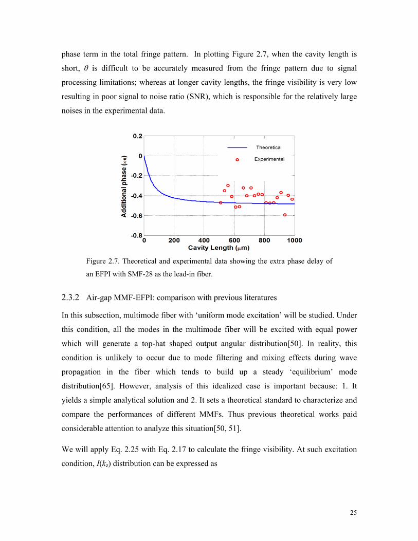
25
phase term in the total fringe pattern. In plotting Figure 2.7, when the cavity length is
short, θ is difficult to be accurately measured from the fringe pattern due to signal
processing limitations; whereas at longer cavity lengths, the fringe visibility is very low
resulting in poor signal to noise ratio (SNR), which is responsible for the relatively large
noises in the experimental data.
Figure 2.7. Theoretical and experimental data showing the extra phase delay of
an EFPI with SMF-28 as the lead-in fiber.
2.3.2 Air-gap MMF-EFPI: comparison with previous literatures
In this subsection, multimode fiber with ‘uniform mode excitation’ will be studied. Under
this condition, all the modes in the multimode fiber will be excited with equal power
which will generate a top-hat shaped output angular distribution[50]. In reality, this
condition is unlikely to occur due to mode filtering and mixing effects during wave
propagation in the fiber which tends to build up a steady ‘equilibrium’ mode
distribution[65]. However, analysis of this idealized case is important because: 1. It
yields a simple analytical solution and 2. It sets a theoretical standard to characterize and
compare the performances of different MMFs. Thus previous theoretical works paid
considerable attention to analyze this situation[50, 51].
We will apply Eq. 2.25 with Eq. 2.17 to calculate the fringe visibility. At such excitation
condition, I(kz) distribution can be expressed as

26
constant, 0<acos asin NA
0, others z
z
k kI k
(2.29)
When inserting Eq.2.29 into Eqs.2.17-2.20, the calculation can be dramatically simplified
by assuming the beam to diverge gently (with small output angle), which helps to drop
the kz terms in the integrations in Eq.2.18 and Eq.2.19 and lead to ν=1 in Eq.2.20. Under
such approximations, Eq.2.17 is transformed to
2 2
0
0
z
kjk
z z
k
z z
I k e dkC S
FVP
I k dk
(2.30)
in which
0
2 cosz z z
k
C I k k k dk (2.31)
0
2 sinz z z
k
S I k k k dk (2.32)
0
2 z z
k
P I k dk (2.33)
The second equation in Eq.2.30 can be demonstrated by inserting Eqs.2.31-2.33 into the
left hand side of the equation followed by some mathematical rearrangement. Inserting
Eq.2.29 into Eq.2.30, and denoting θd=asin(NA) (NA is the numerical aperture of the
MMF), the fringe visibility is analytically expressed as
cos
sinc1 cos 2
z
d
kjk
z
k
d
e dk
FVk
(2.34)

27
where 1 cos
2dk
, Δ is the OPD of the FP cavity. Eq. 2.34 is in complete
agreement with Eq.8 in Ref.[50], the deduction of which is based on ray-optics. Eq. 2.34
predicts that under ‘uniform mode excitation’ condition, the visibility curve is solely
determined by the numerical aperture of the fiber. In Ref.[51], the authors analyzed three
types of fibers, whose parameters are listed in Table 2.1.
Table 2.1. MMF Parametersa.
Parameter Fiber
1 2 3
2a (μm) 100 50 50
n1 1.448 1.448 1.448
n2 1.440 1.416 1.440
NA 0.15 0.30 0.15
V number 30.80 30.68 15.40
aNumbers obtained from Appl. Opt. 43,4659 (2004)
Fiber 1 and 3 have the same NA but fiber 1 has a much larger mode volume; fiber 1 and 2
have similar mode volumes, but the NA of fiber 2 is twice that of fiber 1. Computer
simulation results based on the exact mode analysis [51] and based on Eq.3.34 are
compared in Figure 2.8. It is clearly shown that the results from the two theories agree
well, except little discrepancies due to inaccuracy of Eq.2.34 induced by the
approximations. The fringe visibility for Fiber 2 drops much faster than Fiber 1 and 3
cases due to its larger NA; in contrast, the visibility curve is not affected directly by mode
volume. Although Fiber 1 has a much larger mode volume, its fringe visibility appears to
be similar to that of Fiber 3; Fiber 2 shows much worse fringe visibility compared to fiber
1, yet they have similar mode volumes.

28
Figure 2.8. Fringe visibility versus FP cavity length for fiber 1,2 and 3, all modes
are equally excited. Simulation is based on Eq.3.34 and the fiber mode analysis
method in [51].
2.3.3 Air-gap MMF-EFPI: simulation and experimental results
We use the system configuration shown in Figure 2.4 for the measurement of the fringe
visibility of MMF-EFPIs. A fiber coupled thermal light source (HL-2000 Tungsten
Halogen Source, Ocean Optics, Inc.) with broadband incoherent radiation was used to
illuminate a multimode fiber (MM-S105/125-22A, Nufern) with core diameter of 105μm
and NA=0.22. We used a 50/50 MMF coupler (MMF:100 μm core, 0.29NA) to replace
the circulator, the extra arm of the coupler was immersed in refractive index matching
fluid for anti-reflection. The signal from the EFPI was recorded using an Optical
Spectrum Analyzer (AQ6315A, Ando Electric Co., Ltd.) with spectral resolution set to 1
nm; the fringe visibilities at 800nm, 1200nm and 1550nm were measured.

29
Figure 2.9. Theoretical and experimental results of the fringe visibilities and
additional phases versus OPD for MMF-EFPI. MMF has core diameter 105μm
and NA=0.22. (a) Measured angular distribution. (b) Calculated I(kz) distribution
based on (a). (c) Fringe visibility versus OPD curve for 800nm, 1200nm and
1550nm light, theoretical and experimental. (d) Additional phase θ versus OPD
for 800nm, 1200nm and 1550nm light, theoretical.

30
Due to mode filtering and mixing, the uniform mode excitation condition discussed in
2.3.2 is rarely satisfied in reality; instead, the power distribution among the excited
modes tends to stabilize during propagation, establishing an equilibrium mode
distribution, and creating a far-field intensity distribution similar to a Gaussian. However,
assuming the angular distribution as Gaussian and use Eq. 2.25 to calculate I(kz) leads to
large errors in the calculated fringe visibility. In fact, the fringe visibility curve is very
sensitive to the shape of the angular intensity distribution; as a result, we used measured
angular distribution to deduce I(kz), based on which the fringe visibility was calculated.
In order to measure the angular distribution, we measured the far-field intensity
distribution using a beam profiler (BP104-IR, Thorlabs, Inc.), the linear intensity
distribution was then mathematically converted to angular distribution by characterizing
the distance between the fiber distal end and the profiler; the I(kz) distribution was then
calculated using Eq.25, fringe visibility was then calculated based on I(kz) and Eqs.2.17-
2.20. In Eq.2.20, light coupling coefficient ν was calculated by[66]
22 tan da a (2.35)
where a is the fiber core radius, and Δ and θd are defined in Eq.2.34. The measured
angular distribution, measured I(kz) distribution and the calculated/measured fringe
visibility curves are plotted in Figure 2.9 (a)-(c) respectively. Figure 2.9 (c) demonstrates
a good agreement between the theory and experiment. The calculated additional phases
(based on Eq.2.16) for the three wavelengths were plotted in Figure 2.9 (d). Due to the
insufficient SNR in the experiment, we were unable to provide reliable measurement
results for the additional phase. From the results, it is interesting to note that both the
fringe visibility and the additional phase are dependent on wavelength. This is a natural
outcome due to the fact that I(kz) varies with wavelength. The same principle shown in
Figure 2.6 also applies here: longer wavelength corresponds to narrower I(kz) distribution,
which implies broader fringe visibility curve.
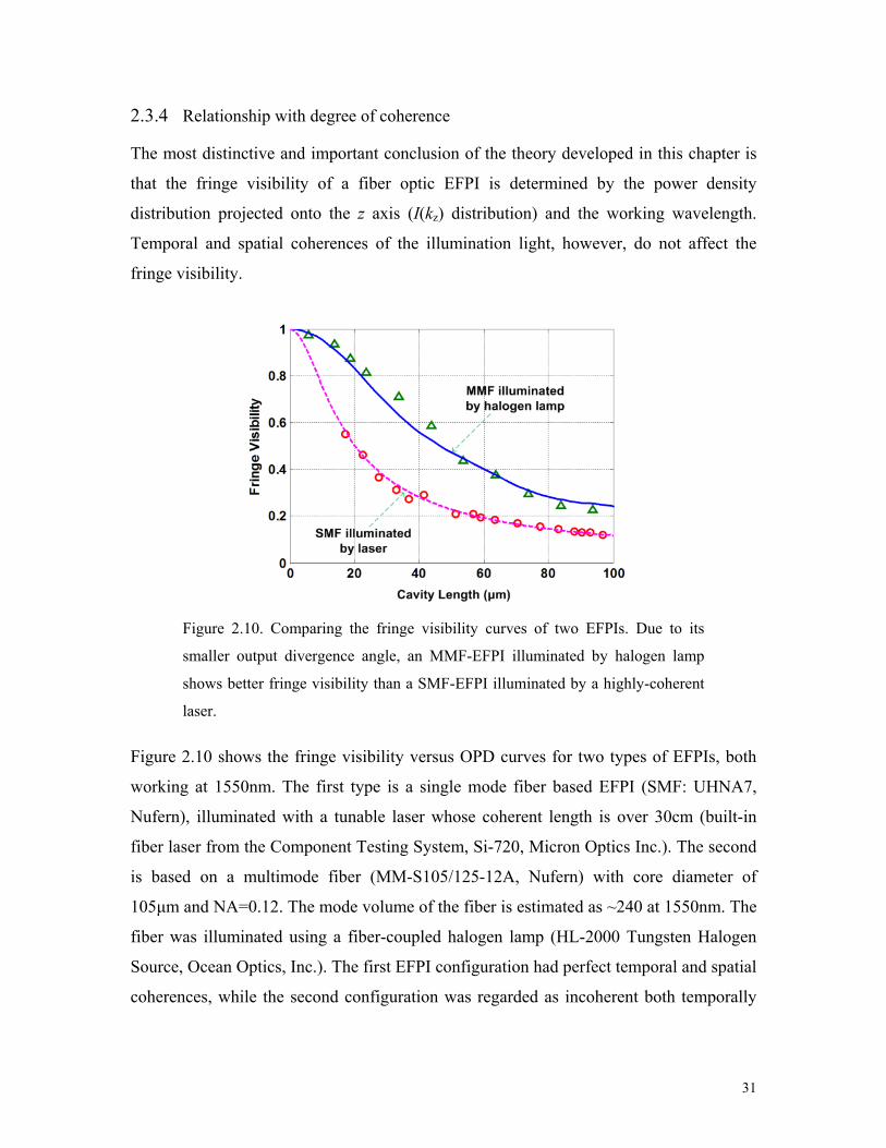
31
2.3.4 Relationship with degree of coherence
The most distinctive and important conclusion of the theory developed in this chapter is
that the fringe visibility of a fiber optic EFPI is determined by the power density
distribution projected onto the z axis (I(kz) distribution) and the working wavelength.
Temporal and spatial coherences of the illumination light, however, do not affect the
fringe visibility.
Figure 2.10. Comparing the fringe visibility curves of two EFPIs. Due to its
smaller output divergence angle, an MMF-EFPI illuminated by halogen lamp
shows better fringe visibility than a SMF-EFPI illuminated by a highly-coherent
laser.
Figure 2.10 shows the fringe visibility versus OPD curves for two types of EFPIs, both
working at 1550nm. The first type is a single mode fiber based EFPI (SMF: UHNA7,
Nufern), illuminated with a tunable laser whose coherent length is over 30cm (built-in
fiber laser from the Component Testing System, Si-720, Micron Optics Inc.). The second
is based on a multimode fiber (MM-S105/125-12A, Nufern) with core diameter of
105μm and NA=0.12. The mode volume of the fiber is estimated as ~240 at 1550nm. The
fiber was illuminated using a fiber-coupled halogen lamp (HL-2000 Tungsten Halogen
Source, Ocean Optics, Inc.). The first EFPI configuration had perfect temporal and spatial
coherences, while the second configuration was regarded as incoherent both temporally
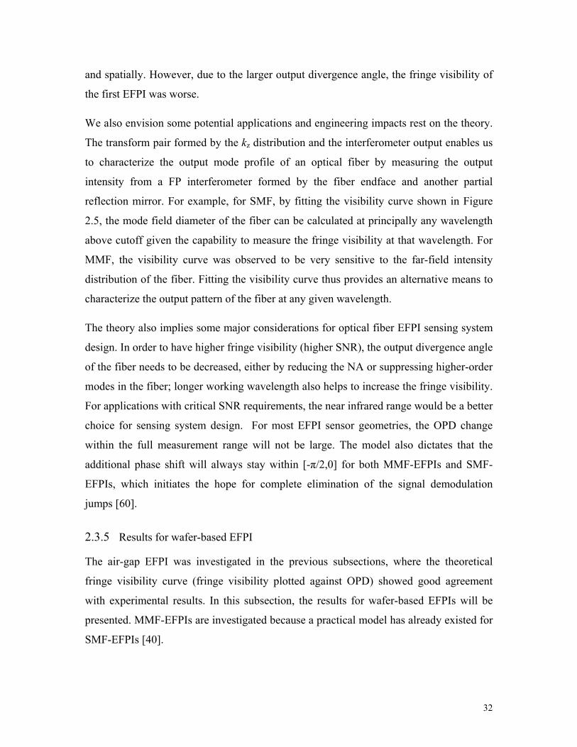
32
and spatially. However, due to the larger output divergence angle, the fringe visibility of
the first EFPI was worse.
We also envision some potential applications and engineering impacts rest on the theory.
The transform pair formed by the kz distribution and the interferometer output enables us
to characterize the output mode profile of an optical fiber by measuring the output
intensity from a FP interferometer formed by the fiber endface and another partial
reflection mirror. For example, for SMF, by fitting the visibility curve shown in Figure
2.5, the mode field diameter of the fiber can be calculated at principally any wavelength
above cutoff given the capability to measure the fringe visibility at that wavelength. For
MMF, the visibility curve was observed to be very sensitive to the far-field intensity
distribution of the fiber. Fitting the visibility curve thus provides an alternative means to
characterize the output pattern of the fiber at any given wavelength.
The theory also implies some major considerations for optical fiber EFPI sensing system
design. In order to have higher fringe visibility (higher SNR), the output divergence angle
of the fiber needs to be decreased, either by reducing the NA or suppressing higher-order
modes in the fiber; longer working wavelength also helps to increase the fringe visibility.
For applications with critical SNR requirements, the near infrared range would be a better
choice for sensing system design. For most EFPI sensor geometries, the OPD change
within the full measurement range will not be large. The model also dictates that the
additional phase shift will always stay within [-π/2,0] for both MMF-EFPIs and SMF-
EFPIs, which initiates the hope for complete elimination of the signal demodulation
jumps [60].
2.3.5 Results for wafer-based EFPI
The air-gap EFPI was investigated in the previous subsections, where the theoretical
fringe visibility curve (fringe visibility plotted against OPD) showed good agreement
with experimental results. In this subsection, the results for wafer-based EFPIs will be
presented. MMF-EFPIs are investigated because a practical model has already existed for
SMF-EFPIs [40].

33
Silica MMF excitation
The silica fiber used in the experiment was a five meter long 0.22 NA MMF
(AFS105/125Y, Thorlabs, Inc.). The optical source was a 850 nm light-emitting diode
(LED), and a beam profiler (BP 104-VIS, Thorlabs, Inc.) was used to capture the far field
power distribution. In calculating the fringe visibility curve, the refractive index of the
wafer cavity was assumed to be 1.77 (representing sapphire). Figure 2.11 (a) shows the
measured angular distribution of the output beam. The distribution resembles a Gaussian
as a result of mode equilibrium, instead of being a top-hat shape. Figure 2.11 (b) shows
the calculated FV curve, according to the measured power distribution. Two features are
distinctive for the wafer cavity: 1) due to the incoherent contribution of the fiber end face
reflection, the fringe visibility is less than unity at OPD equals to zero, in contrast to the
air-gap cavity. 2) At larger OPD, the visibility of the wafer cavity drops much slower,
resulting in higher fringe visibility. This is a natural manifestation of the focusing effect
described in Eq. 2.26.
Figure 2.11. Visibility curve calculation: (a) Measured beam angular distribution
from a 0.22 NA silica fiber. (b) Calculated fringe visibility for both air-gap and
wafer FP cavities based on the characterized angular distribution.
Sapphire fiber excitation
Fiber-optic sensors based on silica fibers generally work below 1000oC due to thermal
diffusion of the dopant and degraded mechanical integrity associated with the high
temperature. Single-crystal optical fibers have demonstrated favorable optical and
mechanical properties under harsh environment, e.g., a sapphire wafer EFPI excited with

34
a single-crystal sapphire fiber was tested to 1600oC without observable signal
degradation [14]. Such single-crystal fibers are typically cladding-less fibers (optical
guidance is supported by air cladding), resulting in extremely high mode volume (e.g.,
for a 75μm diameter sapphire fiber the V number at 850 nm is ~400, resulting in a mode
volume ~66000). The large number of excited modes impose tremendous computational
complexity if exact fiber modal analysis ([51]) is to be employed, rendering such an
approach unpractical. The ray-optics-based approach [50], on the other hand, is over
simplified in which fiber mode mixing and filtering are completely neglected, and could
only be applied when the output angular distribution resembles a top-hat shape (a
condition rarely satisfied in real applications).
Figure 2.12. Visibility curve calculation: (a) Comparison of measured beam
angular distribution from a sapphire fiber and a 0.22 NA silica fiber. (b) Fringe
visibilities of a sapphire wafer EFPI with sapphire fiber and 0.22 NA silica fiber
excitations, calculated based on the characterized angular distribution in (a).
The theory is extremely powerful in modeling the sapphire fiber based EFPI, as the only
required input parameter is the far field power distribution. Once the distribution is
obtained, it is inserted into Eqs. 2.15~2.20 to directly predict the fringe visibility and
additional phase in the spectrum at a given OPD value. Figure 2.12 (a) compares the
measured angular distribution of light outputting from a sapphire fiber (75 μm thick, 50
cm long, excited by a 105/125 μm 0.22 NA silica fiber) and a 105/125 μm 0.22NA silica
fiber. It should be noted that the distributions exhibit significant differences: the silica
fiber has a bell-shape (Gaussian) angular distribution with a cut-off at ~0.25, representing

35
its numerical aperture. The sapphire fiber, having a NA > 1 (full angle acceptance) and
excited by the 0.22NA fiber, shows a significantly modified angular distribution, with
both concentration towards small angle and extension into larger angles. The power
redistribution exhibited by the sapphire fiber is a manifestation of strong mode mixing
and filtering within the waveguide. The difference in the angular distribution results in
slight divergence of the fringe visibility curves, as shown in Figure 2.12 (b).
2.3.6 Influence on WLI-based signal processing
As shown in Eq. 2.16, the additional phase term in the spectrum is a function of OPD,
instead of being a constant as assumed in many WLI-based signal processing algorithms.
Assuming a constant phase, while in reality it is not would eventually lead to abrupt
demodulation jumps. A similar case has been analyzed for intrinsic FP interferometers
(see 3.4.2, 4.2.2). This implies one must be very careful when making the constant phase
assumption to avoid the demodulation jumps. As will be discussed in the following two
subsections, the constant additional phase assumption is theoretically safer for the air-gap
EFPI than the wafer-based EFPI.
Air-gap EFPI
With the measured angular distribution, the additional phase at any given OPD is
straightforwardly calculated from Eq. 2.16. Using an air-gap EFPI excited by the 0.22
NA MMF (AFS105/125Y, Thorlabs, Inc.) whose output angular distribution is depicted
in Figure 2.11 (a), the additional phase evolution as a function of OPD is plotted in
Figure 2.13 (a), solid curve. The measured additional phase was drawn in the same plot
as triangles. It is observed that for EFPI, as long as the OPD change stays small during
the full measurement range, the change of the additional phase is negligible (well below
0.5π), and the dominate contribution to a potential jump is the demodulation noise. Thus,
provided the signal to noise ratio is high and fringe order estimation is accurate, assuming
a constant additional phase for the air-gap based EFPI is secure.
Wafer-based EFPI
Similar to the air-gap EFPI, the OPD-dependent additional phase change is also small for
the wafer-based EFPI. However, the temperature-dependent material dispersion will
introduce another phase term which evolves with OPD. For the spectrometer being used
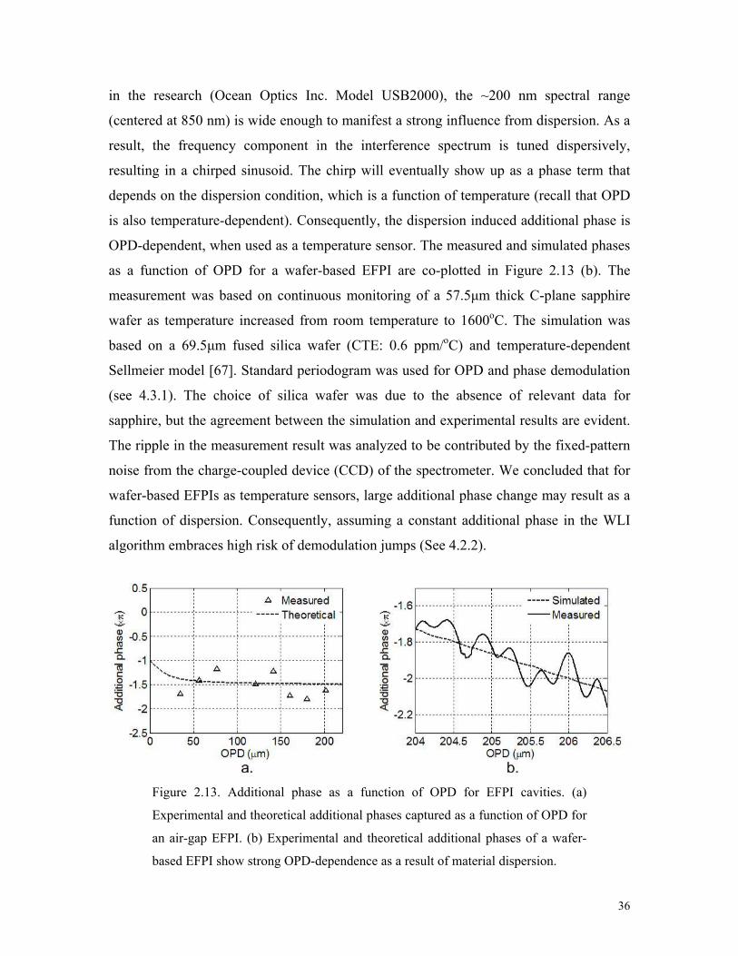
36
in the research (Ocean Optics Inc. Model USB2000), the ~200 nm spectral range
(centered at 850 nm) is wide enough to manifest a strong influence from dispersion. As a
result, the frequency component in the interference spectrum is tuned dispersively,
resulting in a chirped sinusoid. The chirp will eventually show up as a phase term that
depends on the dispersion condition, which is a function of temperature (recall that OPD
is also temperature-dependent). Consequently, the dispersion induced additional phase is
OPD-dependent, when used as a temperature sensor. The measured and simulated phases
as a function of OPD for a wafer-based EFPI are co-plotted in Figure 2.13 (b). The
measurement was based on continuous monitoring of a 57.5μm thick C-plane sapphire
wafer as temperature increased from room temperature to 1600oC. The simulation was
based on a 69.5μm fused silica wafer (CTE: 0.6 ppm/oC) and temperature-dependent
Sellmeier model [67]. Standard periodogram was used for OPD and phase demodulation
(see 4.3.1). The choice of silica wafer was due to the absence of relevant data for
sapphire, but the agreement between the simulation and experimental results are evident.
The ripple in the measurement result was analyzed to be contributed by the fixed-pattern
noise from the charge-coupled device (CCD) of the spectrometer. We concluded that for
wafer-based EFPIs as temperature sensors, large additional phase change may result as a
function of dispersion. Consequently, assuming a constant additional phase in the WLI
algorithm embraces high risk of demodulation jumps (See 4.2.2).
Figure 2.13. Additional phase as a function of OPD for EFPI cavities. (a)
Experimental and theoretical additional phases captured as a function of OPD for
an air-gap EFPI. (b) Experimental and theoretical additional phases of a wafer-
based EFPI show strong OPD-dependence as a result of material dispersion.
37
2.4 Conclusion
A theoretical effort to model the interference spectra of low finesse fiber optic Fabry-
Perot interferometers is presented in the chapter. The deduction of the theory was based
on a rigorous diffraction treatment of the field in the FP cavity, and through some
reasonable approximations, we reached a transform pair between the interferometer
output and the spatial power density distribution projected onto the direction normal to
the reflection mirrors. After some further approximations, it was found that the above
relationship reduced to a Fourier-transform problem, which was analogous to the Fourier
transform pair formed by the output intensity of a Michelson interferometer and the
spectrum of the optical source used to illuminate the interferometer. The theory was
experimentally proven using both single-mode fiber and multimode fiber based EFPIs,
and we sought to establish relationships between the new model with previously
published theoretical approaches. We found that the fringe visibility and additional phase
in the interferogram were strongly influenced by the output spatial power density
distribution and working wavelength, but were not directly related to either temporal or
spatial degree of coherence. We further analyzed the visibility curves of a wafer-based
EFPI, excited with different fibers. According to the model, different excitation condition
results in quite distinctive features of the visibility curve, and maximizing the fringe
contrast relies on designing the excitation to yield a minimized beam divergence. At last,
we analyzed the OPD-dependent additional phase terms separately for air-gap and wafer-
based EFPIs, and found that in principle, the additional phase of an air-gap cavity
changes very moderately while that of a wafer-based cavity is dominantly affected by
material dispersion.

38
Chapter 3 Modeling of Fiber Optic Low-Finesse IFPI Sensors
3.1 Introduction
The Single-/multi-/single mode (SMS) fiber optic structure is formed by fusion splicing a
section of multimode (MMF) fiber sandwiched into a single-mode fiber (SMF) link [68].
When used in transmission mode, such structures are applied as sensors, filters,
modulators, switches, and fiber lenses [69-77], and both step-indexed (SI-) [76, 78] and
graded-indexed multimode fibers (GI-MMF) [72, 79] have been studied in the past. In
these configurations, modal interference plays a central role in generating desired
interference signal.
Figure 3.1. Schematic of the SMS-IFPI sensor.
When used in reflection mode, the SMS structure is typically referred to as a (low-finesse)
fiber optic intrinsic Fabry-Pérot interferometer (IFPI) [80, 81]. The desired interference is
formed by the two reflections generated at the splicing boundaries. The sinusoidal sensor
signal is suitable for harmonic-analysis-based signal processing, in which multiple IFPIs
with various cavity lengths can be fabricated along a single fiber-optic link. Each sensor
contributes to the total spectrogram a harmonic component with distinct frequency
defined by its cavity length [27, 80]. The subject of the work is GI-MMF based SMS-
IFPI sensor (IFPI infers reflection mode, see Figure 3.1). Through a combination of
analysis and experimentation, this work presents a comprehensive picture of the SMS-
IFPI sensor structure. A variety of design considerations are addressed to optimize sensor
strength, SNR, transmission loss, multiplexing capability, and signal stability.
The first consideration in IFPI is the compromise between SNR and sensor mechanical
integrity. This chapter addresses these practical design issues by presenting an analytical

39
solution for reflectivity at the splicing junction for a given refractive index transition
width.
It is well accepted that the SMS-IFPI sensor has the potential for very low transmission
loss due to the selective modal excitation in the MMF [70]. However, sensors reported to
date have exhibited high transmission loss (roundtrip about -3dB on average), which
contradicts the established belief. The loss results in an attenuation of almost 20dB
through 6 inline sensors, yielding an insufficient signal-to-noise ratio (SNR) for any
additional sensors to be multiplexed. In 2003 Kumar et al. attributed this insertion loss
problem to the large mismatch between the fundamental modes of SMF and MMF [72].
Practically the roundtrip insertion loss needs to be reduced to below 1 dB in order to
multiplex ten sensors.
On the other hand, modal interference in GI-MMF has been employed to fabricate a
variety of fiber optic lenses and collimators since 1987 [82-85]. This work expands on
the principle of a gradient-index lens, using controlled modal interference to dramatically
reduce sensor insertion loss. Section 3.2.2 contains a rigorous analysis of cavity
refocusing using both the traditional ray matrix approach and fiber mode theory. Though
experimentation (Sections 3.2.3), the resulting optimized IFPI sensor demonstrated
greatly reduced roundtrip loss below 0.5 dB. A novel multiplexing scheme, based on the
analysis results of multiple MMF types, is presented in 3.2.3. Modal interference is
shown to complicate the sensor signal, obscuring the sinusoidal Fabry-Pérot fringe
pattern. The issue of modal interference is analyzed to shed light on IFPI sensor signal
demodulation, as will be discussed in 3.3.
3.2 Basic models for sensor reflection and transmission
3.2.1 Reflectivity of the cavity mirrors
The upper bound of the reflectivity of a planar splicing surface can be roughly estimated
by the Fresnel reflection formula [86]
2
1 2
2
1 2
n nR
n n
(3.1)

40
where n1 and n2 are the highest refractive indices of the fiber cores. During a real fusion
splice process, the extremely high temperature and finite arc duration give rise to
diffusion of the dopant across the splicing plane, which tends to smear any index
difference across the boundary, thus reducing reflectivity. In order to model the complex
index profile, numerical methods have been used [86]. Here we consider a simple
analytical solution to show how the reflectivity decreases with widening index transition
length.
Suppose a complex index distribution along the fiber axis n(z), and assume the index is
uniform on the fiber cross section for any given z. For the above index profile, at location
z the amplitude reflectivity is given by Eq.3.1. Assuming the total change of n is small,
r(z) = n’(z) dz/2n(z), where n’(z) = dn/dz is the changing rate of n with respect to z. Let z
= 0 represent the point at which the total reflected field is detected, and the field reflected
at z = z0 will pick up a phase term exp[-j2βz0] at z = 0. The term β denotes the optical
propagation constant in the fiber (here for simplicity the fiber is assumed to be single-
mode). The total field reflectivity, defined by the ratio between the reflected field and the
input field at z = z0 can thus be expressed as
2j
tot
zr m z e dz
(3.2)
where ( ) '( ) / 2 ( )m z n z n z and the power reflectivity is found by R = |rtot|2. Eq. 3.2 shows
the Fourier transform (FT) relationship between m(z) and rtot. It should be noted that such
mathematical relationship has been used for frequency domain distributed sensing [8].
The reflection spectrum of an IFPI with finite index transition length is modeled by
applying Eq.3.2 and some basic properties of FT.
The splice point with diffusion-induced finite transition width is modeled by a half-period
cosine function, and the index profile along the z-axis of an imperfect IFPI is shown in
Figure 3.2 (a). The FP cavity length is L, the transition width is Δ, and the total index
change is δn. The corresponding m(z) distribution is calculated and shown in Figure 3.2
(b). This distributed reflectivity profile can be represented as the convolution of two
functions (f1 * f2) (z), where f1 is a rectangular-windowed cosine (Figure 3.2 (c)), and f2 is

41
formed by two Dirac delta functions at L/2 with amplitude (-/+) unity (Figure 3.2 (d)).
The above procedure assumes a constant n in the denominator of m, which is reasonably
accurate for small index changes. The final power spectrum, by using Eq.3.2 and some
mathematical manipulations, is
22
2 1 cos 22 4
nI L
n
(3.3)
where =sinc / 2 sinc / 2x x x and sinc(x) = sin(x)/x. The result is shown in
Figure 3.3, in which the relative reflectivity (reflectivity normalized to the maximum
reflectivity defined in Eq.3.1) is plotted as a function of the transition width Δ for three
different wavelengths. n is assumed to be 1.46. When the transition length approaches λ/2
(λ being the vacuum wavelength), the reflectivity drops more than 20 dB from its
maximum value.
Figure 3.2. Computation procedure to calculate m(z) for the index profile shown
in (a). The m profile, shown in (b), can be decomposed as a convolution of the
functions shown in (c) and (d).
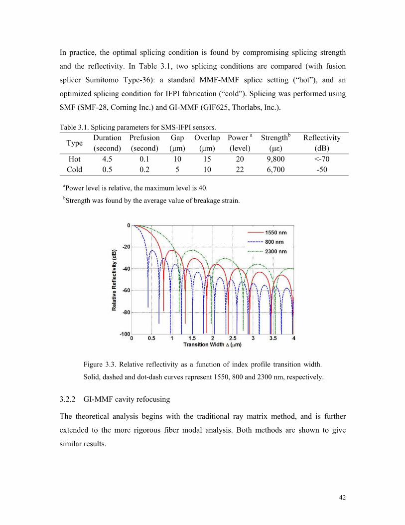
42
In practice, the optimal splicing condition is found by compromising splicing strength
and the reflectivity. In Table 3.1, two splicing conditions are compared (with fusion
splicer Sumitomo Type-36): a standard MMF-MMF splice setting (“hot”), and an
optimized splicing condition for IFPI fabrication (“cold”). Splicing was performed using
SMF (SMF-28, Corning Inc.) and GI-MMF (GIF625, Thorlabs, Inc.).
Table 3.1. Splicing parameters for SMS-IFPI sensors.
Type Duration Prefusion Gap Overlap Power a Strengthb Reflectivity (second) (second) (μm) (μm) (level) (με) (dB)
Hot 4.5 0.1 10 15 20 9,800 <-70 Cold 0.5 0.2 5 10 22 6,700 -50
aPower level is relative, the maximum level is 40. bStrength was found by the average value of breakage strain.
Figure 3.3. Relative reflectivity as a function of index profile transition width.
Solid, dashed and dot-dash curves represent 1550, 800 and 2300 nm, respectively.
3.2.2 GI-MMF cavity refocusing
The theoretical analysis begins with the traditional ray matrix method, and is further
extended to the more rigorous fiber modal analysis. Both methods are shown to give
similar results.

43
The ray matrix approach adopts the treatment by Emkey and Jack [82]. The modeling
process begins with the complex q parameter of a Gaussian beam with curvature radius
RC(z) and beam radius ω(z)
2
1 1
C
iq z R z z n
(3.4)
The q parameter at the SMF-MMF boundary is defined as q1, and the input field is the
LP01 mode of the SMF. The planar wavefront at the z = 0 splice interface requires
RC(0)∞. In order to calculate the q parameter in the MMF at z = l, the transformation is
readily obtained by
2 1 1q Aq B Cq D (3.5)
the elements A, B, C and D are determined by the GI-MMF through
1cos sin
sin cos
gl glA Bg
C Dg gl gl
(3.6)
where the g parameter is defined as
MMF
ga
(3.7)
where δ = 1-(n2 / n1)2, (notice δ is twice the value of the fractional refractive index
difference), in which n1 and n2 denote the maximum refractive index of the MMF core,
and the refractive index of the MMF cladding, respectively; aMMF denotes the radius of
the GI-MMF core. Inserting Eq.3.4 into Eq.3.5 and applying RC(0)∞ for q1, we get
2
1A iB
q l (3.8.1)
2 4 2 2
0 1
2 2 2 4 2 2 2
0 1
sin cos
sin cos
g n g gl glA
gl n g gl
(3.8.2)

44
2 2
0 1
2 2 2 4 2 2 2
0 1sin cos
n gB
gl n g gl
(3.8.3)
where ω0 is the Gaussian beam radius of the SMF LP01 mode. In seeking of the position
where planar wavefront along the MMF is located, we set A = 0 and find two sets of
solutions for l
rl Ng
, where N = 1,2,3, … (3.9.1)
1
2cl N
g
, where N = 1,2,3,… (3.9.2)
For the first set of solutions (lr), substitution into Eq.3.8.3 yields a spot radius equal to ω0,
which is identical to that of the SMF fundamental mode. We refer such locations as
“refocusing points”. The second set of solutions (lc), when inserted into Eq.3.8.3 gives
rise to a spot radius of
0 1
ln g
(3.10)
It can be easily shown that ω(l) ≈ (NASMF/NAMMF)aMMF, where NASMF and NAMMF are
the numerical apertures of SMF and MMF. For typical GI-MMF, the value of Eq.3.10 is
approximately 2~3 times of ω0. We refer lC as “collimating points”, which are employed
to fabricate fiber lenses.
Equations 3.9.1 and 3.9.2 imply a series of periodic focusing and defocusing when light
propagates in a SMF-excited GI-MMF. For an SMS-IFPI, when the cavity length is cut to
the neighborhood of lr (Eq. 3.9.1), light in the FP cavity is refocused into the lead-out
SMF, leading to minimum transmission loss. On the contrary, when the FP cavity has a
length near to lc (Eq. 3.9.2), due to the significant mode field diameter (MFD) mismatch,
coupling of the cavity mode into the lead-out fiber can be very lossy.
In reality, periodic refocusing effect only exists at the beginning of the MMF section
(within several centimeters), and the pattern becomes increasingly blurry along the fiber.

45
The periodicity is dictated by the “beating” of the excited modes (as will be discussed
below), and eventually all the modes become desynchronized during propagation. In
order to better understand and more accurately analyze such phenomena, fiber modal
analysis is necessary.
For the GI-MMF whose index profile is radially parabolic, the transverse mode profile
can be well approximated by the Laguerre-Gaussian function [87]. If the MMF is excited
by standard SMF, modes with azimuthal index other than zero (LPνμ mode, ν≠0)
annihilate due to mode orthogonality, which greatly simplifies the following analysis. In
this case the mode profile can be expressed as
2
2
1
2 21 2r
r Ae L
(3.11)
with an effective Gaussian spot size defined through
2
1
0 1
2 MMFa
k n
(3.12)
and the mode number μ = 0,1,2,…. In Eq.3.11 ρ denotes radial coordinate and Lμ is the
Laguerre polynomial of degree μ. The constant A is calculated by mode power
normalization:
2
01d
(3.13)
The effective refractive index for mode μ is found to be
1/ 2
, 1
0 1
21e
MMF
n n Mk n a
(3.14)
where M = 2μ+1 and the propagation constant is defined by βμ = k0 ne,μ. The mode
functions in Eq.3.11 are orthogonal, and the LP01 mode of the SMF may couple into
multiple core modes of the MMF at the first splicing plane. The field in the MMF is thus
decomposed into the orthogonal modes as

46
1
0
N
MMF c
(3.15)
ψMMF is the field profile in the MMF, N is the total number of modes excited, and the
coupling coefficients cμ are found by the overlapping integral:
*
0 SMFc d
(3.16)
where ψSMF is the normalized field profile of the SMF LP01 mode. The field profile at any
location along the MMF (assume z = 0 is the first splicing plane) is found by summing
the individual orthogonal modes:
1
0
expN
z c j z
(3.17)
Table 3.2. Fiber parameters used for the simulation.
Fiber Type Core Cladding Core Cladding
δ (%)
Diameter (μm)
Diameter (μm)
Index (RIU)
Index (RIU)
SMF 8.4 125 1.4504 1.4447 0.78 MMF1 50 125 1.4760 1.4615 1.96 MMF2 62.5 125 1.4760 1.4500 3.49
Table 3.3. Power coupling coefficients of five MMF modes
Fiber 1 2 3 4 5
LP00 LP01 LP02 LP03 LP04 MMF1 0.8259 0.1115 0.0413 0.0132 0.0051 MMF2 0.8457 0.1002 0.0371 0.0108 0.0040
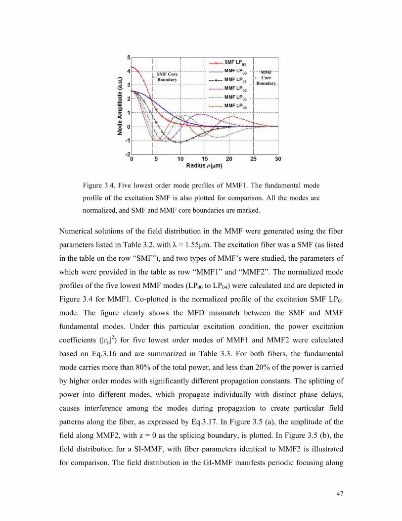
47
Figure 3.4. Five lowest order mode profiles of MMF1. The fundamental mode
profile of the excitation SMF is also plotted for comparison. All the modes are
normalized, and SMF and MMF core boundaries are marked.
Numerical solutions of the field distribution in the MMF were generated using the fiber
parameters listed in Table 3.2, with λ = 1.55μm. The excitation fiber was a SMF (as listed
in the table on the row “SMF”), and two types of MMF’s were studied, the parameters of
which were provided in the table as row “MMF1” and “MMF2”. The normalized mode
profiles of the five lowest MMF modes (LP00 to LP04) were calculated and are depicted in
Figure 3.4 for MMF1. Co-plotted is the normalized profile of the excitation SMF LP01
mode. The figure clearly shows the MFD mismatch between the SMF and MMF
fundamental modes. Under this particular excitation condition, the power excitation
coefficients (|cμ|2) for five lowest order modes of MMF1 and MMF2 were calculated
based on Eq.3.16 and are summarized in Table 3.3. For both fibers, the fundamental
mode carries more than 80% of the total power, and less than 20% of the power is carried
by higher order modes with significantly different propagation constants. The splitting of
power into different modes, which propagate individually with distinct phase delays,
causes interference among the modes during propagation to create particular field
patterns along the fiber, as expressed by Eq.3.17. In Figure 3.5 (a), the amplitude of the
field along MMF2, with z = 0 as the splicing boundary, is plotted. In Figure 3.5 (b), the
field distribution for a SI-MMF, with fiber parameters identical to MMF2 is illustrated
for comparison. The field distribution in the GI-MMF manifests periodic focusing along

48
the z axis, whereas the field in the SI-MMF is rather complex. The reason causing this
disparity lies in a special relationship among the MMF propagation constants, as
discussed below.
Figure 3.5. Light propagation in multimode fibers. (a) Field amplitude
distribution in GI-MMF (MMF2). (b) Field amplitude distribution in SI-MMF,
whose parameters are identical to MMF2.
The periodic focusing effect in GI-MMF gives rise to periodic transmission loss. An
investigation of the loss using fiber mode theory gives a clearer physical interpretation of
the refocusing phenomenon. The coupling loss of the MMF can be expressed as [78]
2
2
1
expN
m mm
z c j z
(3.18)
where m = μ + 1. Through binomial expansion of Eq.3.14, the difference between two
neighboring values of the effective refractive index is calculated as:

49
, , 1 02n e n e n MMFn n k a (3.19)
Inserting Eq.3.19 into Eq.3.18 leads to
2
2
01
exp 1N
m nm
z c j m k z
(3.20)
With some mathematical manipulations, the loss is obtained as
1
01
expN
p np N
z jpk z
(3.21)
in which the expansion coefficient is expressed as
2
p n mn m p
c c
(3.22)
As clearly shown in 3.21, the z dependent transmission loss is a Fourier series with
fundamental angular frequency k0Δn, which predicts the spatial period as
0
2 MMF
n
a
k g
(3.23)
The periodicity shown in Eq.3.23 is in complete agreement with the one deduced by the
ray matrix method as in Eq.3.9.1. In fact the effective index relationship in Eq.3.19
dictates a spatial frame with which the field repeats itself according to the Fourier series
Eq.3.21; this serves as an alternative interpretation of the refocusing effect. In applying
Eq.3.19, only the first two terms in the expansion of Eq.3.14 are retained. However,
neglecting the higher order terms in Eq.3.14 will eventually cause significant error at
larger z, and the Fourier series in Eq.3.21 will fail. Thus the refocusing can only held for
a certain distance before reaching an unfocused equilibrium state, which, together with
the decay of the leaky modes, sets up a steady-state propagation within centimeters [88].

50
3.2.3 Verification of the refocusing model
Insertion loss reduction by cavity refocusing
To verify the theory in Section 2B, standard SMF (SMF 28e, Corning Inc.) was fusion
spliced to a section of MMF (InfiniCor600, Corning, Inc.) and re-spliced back to the
lead-out SMF. According to the technical specs, the MMF is similar to MMF1 in Table
3.2. The transmission loss of the device was characterized as a function of the MMF
length. For the fusion splicing, we used both of the splicing conditions in Table 3.1.
Figure 3.6. Calculated and experimental results for the coupling loss and beam
radius of the GI-MMF. (a) Coupling loss variation as MMF length and (b) Beam
radius variation as MMF length. For the simulation, the MMF1 fiber is selected.
Corning InfiniCor600 was used for the experiment.
For comparison, we used both the ray matrix method and the fiber modal analysis to
determine the transmission loss and the beam radius of MMF1. The calculated and
measured transmission loss (one-way) are co-plotted in Figure 3.6 (a). Notice the splicing
condition does not strongly affect the transmission loss, in contrast to its influence on the
reflection. In Figure 3.6 (b), the calculated beam radius, using both ray matrix and modal
analysis, are shown to have good agreement. We also compared the calculation result to

51
the experimental result published in [84], in which the fiber is cut to designed length for
beam collimation. The beam spot size shown in the figure in green circle was deduced
from the divergence angle as reported in the paper.
The influence of the loss reduction on sensor signal demodulation was further studied
with real sensors. A link with ten IFPI sensors was fabricated using standard SMF and a
GI-MMF (GIF625, Thorlabs Inc.). The MMF selected has fiber parameters similar to that
of MMF2 as listed in Table 3.2. Based on simulation results, the refocusing length was
determined to be 517μm, according to Eq. 3.9.1. Subsequently, the cavity lengths of the
sensors were cut to multiples of 517μm to minimize the transmission loss. The spectrum
of the link was interrogated using a swept-laser spectrometer (Si-720, Micron Optics Inc.)
which offered 20,000 interrogation points from 1520 to 1570nm spectral range. All the
sensors were co-located inside a furnace and temperature calibration was performed. The
calibration curve was fitted with a third-order polynomial, and the fitting error was
characterized by its standard deviation as an estimation of the 1-σ estimation error.
Notice that the calibration was based on calculating the OPD of the sensors, and we used
the “direct OPD” approach, as elaborated in [60], Eq. 21, for the signal demodulation.
For comparison, another link with six sensors was fabricated and tested. Instead of
having controlled length to minimize the transmission loss, the sensors were cut into
lengths in rough multiples of 1000 μm (from 1000 to 6000um). The link had significantly
increased transmission loss (roundtrip loss averaged nearly 3dB per sensor), in vivid
contrast to the first link whose average loss was <0.5 dB per sensor. This is clearly shown
in the Fourier transform of the sensor spectra in Figure 3.7 (a), where the harmonic peaks
due to each individual sensor are visible.
In Figure 3.7 (b), the relative OPD estimation error (normalized to OPD) for the sensors
in both links is plotted. While the sensors in link 1 demonstrate no quality reduction
toward the end of the link, the last three sensors in the non-optimized link show
dramatically increased inaccuracy as a result of reduced SNR. A natural benefit from the
loss reduction is an increase in multiplexing capacity.

52
Figure 3.7. Experimental results showing the benefit of IFPI cavity length control.
In (a), the FFT of the spectra for a link with (solid) and without (dashed)
refocusing are compared. The relative OPD estimation error for each sensor in
the links is plotted in (b).
Increasing the multiplexing capacity
As discussed in 3.2.2, by controlling the SMS-IFPI cavity lengths, the roundtrip insertion
loss of each sensor can be reduced to less than 0.5dB. For a twenty-sensor link, this
results in a total insertion loss of less than 10dB, which is sufficient for reliable
demodulation of all the sensors. However, this requires some of the sensors to have very
long cavity lengths: the twentieth sensor will have a cavity length exceeding 1 cm. Such
long cavity length tends to impose signal demodulation challenges stemming from
environmental fluctuations. To address this problem, different types of MMF can be
employed. Table 3.4 lists some key properties of three types of GI-MMF. The diverse
optical properties of different MMFs lead to distinct pitches, allowing multiplexing of
more than twenty sensors with a maximum cavity length of around 6 mm. The designed

53
cavity lengths should bear enough separation to allow minimum crosstalk and enough
dynamic range. Figure 3.8 conceptually illustrates a potential design.
Table 3.4. Key properties of three types of MMF.
Fiber NA Δ (%) Pitch (μm) Theoretical
Pitch (μm) Measured
GIF625 0.275 1.8 517 520 InfiniCor600 0.200 1.0 555 563 OFS100/140 0.298 2.1 764 840
Figure 3.8. Design of a sensing link with 22 IFPI sensors multiplexed with three
different types of MMF. 62.5/125 MMF: Thorlab GIF-625; 50/125 MMF:
Corning InfiniCor600; 100/140 MMF: OFS-100/140.
3.3 Analysis of the IFPI additional phase
Whitelight interferometry has been proven to be perhaps the most practical way for the
demodulation of fiber F-P sensors. Typical signal demodulation aims at finding the
optical path difference (OPD, defined as OPD = 2nL, where n is the refractive index and
L is the physical length of the cavity) according to the sinusoidal spectral information
given by [27, 39, 89] :
~ cosI k OPD (3.24)
In the above formula the DC component has been removed already. The sinusoidal nature
of the spectrum comes from the interference generated by the two cavity mirrors, k is
equal to 2π/λ where λ is the light wavelength in vacuum, the term π comes from the

54
reflection from an optically denser medium, and the term φ is an additional phase term,
which has been investigated in the case of SMF-EFPI and MMF-EFPI by Han et al. [40,
52] and further in chapter 2 (2.3.6). This additional phase term is explained as a result of
wave-front distortion of the light during propagation in free-space. The OPD
demodulation accuracy can be greatly enhanced by measuring the additional phase term φ
in advance (the so-called OPD demodulation with known phase), which requires the
phase term to be a constant for any given FP cavity [27]. In reality, the phase term is
dependent on the cavity length in EFPI [40] and is also dependent on the mode-field
distribution (MFD) in the lead-in multimode fiber for MMF-EFPI [52] (the dependence is
further analytically expressed by a transform of I(kz) as in chapter 2), which means one
needs to be very careful before assuming the phase term to be constant during OPD
measurement. In this subsection, by taking into account the overall effect exerted by the
multiple transmission modes in the cavity, we analyzed the interference spectrogram of
SMS-IFPI sensor and concluded that a non-constant phase term also existed. Similar to
the EFPI case, the phase term was generated by the field wave-front distortion, yet for
EFPIs the distortion comes from free space propagation while for IFPIs it is a side effect
of inter-modal dispersion.
3.3.1 Modal analysis of the SMS-IFPI
Exact field expression
A typical SMS-IFPI sensor is illustrated in Figure 3.1. Instead of applying Eq.3.24 to
obtain the sensor spectrum, a more accurate model employs analysis of modal coupling
and propagation in the multimode waveguide [51, 72, 90, 91]. Light in the SMF is carried
by LP01 mode of SMF with normalized mode profile Φ0. At the interface R1, the mode
energy is split into several parts carried separately by LP0k modes with normalized mode
profile Φk in the MMF (here we made the assumption that the MMF is weakly guided,
step-index fiber for simplicity of analysis). Modes in the MMF with azimuthal number
other than zero will not be exited due to mode orthogonality. For each mode, the coupling
coefficient is defined as1
*0 0k k
R
dxdy . Being reflected by R2 and propagating to R1,
the k’th mode profile can be expressed as 0 exp 2 /k k kr j OPD , where

55
2k kOPD n L , kn is the effective index of the k’th mode. At interface R1, all these modes
will be re-coupled into the fundamental LP01 mode of the single mode fiber with coupling
coefficient1
* *0 0 0k k k
R
dxdy . As a result, the contribution to the total mode
profile by each mode can be described as2
0 0
2expk kr j OPD
, and the total
field profile at R1 can be expressed as:
20
1
21 exp
N
s k kk
r j OPD
(3.25)
where 0k k is a real number and N modes are assumed to be excited in the MMF.
Based on the expression for the total field above, we can find the reflection intensity from
the sensor as:
1
2* 2 1s s
R
I dxdy r (3.26)
where 2
1
2exp
N
k kk
j OPD
is an effective vector to be discussed in more
details in the following section. Also we have already applied the normalization condition
1
*0 0 1
R
dxdy . Note that if only one mode is excited in the MMF, Eq.3.26 will be
automatically reduced to Eq.24 after canceling the DC component.
Two-mode excitation
The expression for the total field intensity deduced from the last section (Eq.3.26) is
comprehensive but relatively complicated. In this section we consider a much simpler
case in which only two modes are excited in the MMF with similar effective refractive
indices; this analysis can provide us with illustrative understanding of how intermodal
dispersion affects the sensor spectrum.

56
Assume that the effective indices of the two modes to be n1 and n2, respectively, and
accordingly the OPD experienced by the two modes to be OPD1=2n1L and OPD2=2n2L,
define 1 2OPD OPD OPD such that OPD2 can be expressed by OPD2 = OPD1-ΔOPD.
The total reflected spectrum can be expressed as
I
4 4 2 2 2 2
1 2 1 1 0 2 1 0 1 2 01 2 cos 2 cos 2 cosOPD k OPD OPD k OPD k
(3.27)
In the above equation, the fourth and fifth terms on the right hand side describe the
interference of the modes with themselves, and the last term accounts for the interference
between the two modes. After some mathematical manipulations, Eq.3.27 can be
rewritten as:
21 0 01 2 sin ,I r OPD k OPD k
Where
4 4 2 21 2 1 2 02 cos OPD k
2 21 2 0
022 0
0 2 21 2 0
022 0
cosarctan ,sin 0
sin,
cosarctan ,sin 0
sin
OPD kOPD k
OPD kOPD k
OPD kOPD k
OPD k
(3.28)
It is not difficult to find that at the limit 2 22 1 (which means the second mode is
excited so weakly that almost all the power is carried by the first mode), Eq.3.28 reduces
to Eq.3.24 with the additional phase term equal to zero. As the second mode emerges, the
amplitude and phase of the sinusoid will be modulated. The phase term 0,OPD k as a
function of 0OPD k has been plotted in Figure 3.9. To plot the figure, the wavelength
span was set from 1400 to 1700 nm, the effective refractive indices of mode 1 and mode

57
2 were set to be 1.448 and 1.441, respectively, the cavity length was set to 1mm, and four
different cases with excitation ratio ( 2 21 2/ ) of 6:4, 7:3, 8:2 and 9:1 were compared.
Figure 3.9. Additional phase term for a two-mode cavity at different excitation ratios.
Rotating vector picture
In the previous section we only considered the excitation of two modes inside the MMF
cavity. In reality, the number of modes excited can be much more, which complicates the
problem. From Eq.3.26, the received intensity is proportional to 2
1 where the vector
is defined as 2
1
2exp
N
k kk
j OPD
. The received power can be expressed
as:
2 2~ 1 1 2 cosI , where (3.29)
Equation 3.29 leads to the conclusion that the total phase in the interference spectrogram
can be directly obtained from the angle of the vector . In the following discussion, for
simplicity without losing generality, we omit the phase term in the expression of vector
:
2
1
2exp
N
k kk
j OPD
(3.30)

58
where 2k kOPD n L , kn is the effective refractive index of the kth mode. It is
straightforward to find out that is the sum of N vectors representing N orthogonal modes
(define mode vector 2 2expk k kj OPD
), the modulus of each vector is the
square of the magnitude of the mode coupling coefficient between the given mode and
the LP01 mode of the SMF; the phase of each vector is simply the product of the vacuum
wavenumber and the effective OPD of that mode. Figure 3.10 illustrates how the total
field vector is related to each individual mode vector. Totally five modes were assumed
to be excited.
Figure 3.10. Relationship between the total field vector and five individual mode
vectors.
In the interference spectrogram, as the wavenumber k increases, all the N individual
mode vectors (υk) will rotate at different angular speed OPDk=2nkL, the mode vector of
the fundamental LP01 mode rotates at the fastest speed (corresponding to the largest
effective refractive index), while the mode vector of LP0N mode rotates the slowest; the
differences among rotational speeds of all the mode vectors are very small because nk’s
have very similar values. Although the individual vectors rotate at similar speeds, their
pointing directions are almost arbitrary because the wavenumber k and the cavity length
L are both very large numbers. The effective vector rotates at a speed that depends
simultaneously on the rotational speed of each vector and their relative orientations. If
most of the mode vectors align at similar directions, the rotating speed of the effective
vector can be slower than any of the individual vectors; there are also occasions where its
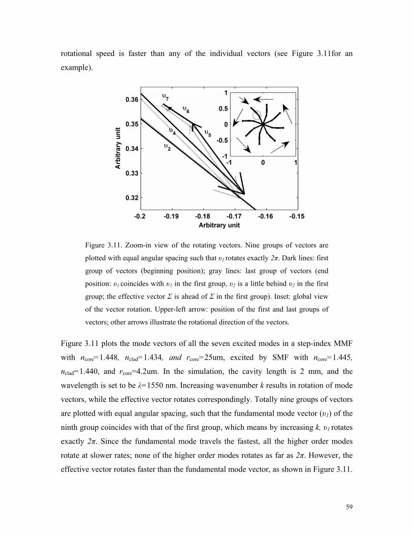
59
rotational speed is faster than any of the individual vectors (see Figure 3.11for an
example).
Figure 3.11. Zoom-in view of the rotating vectors. Nine groups of vectors are
plotted with equal angular spacing such that υ1 rotates exactly 2π. Dark lines: first
group of vectors (beginning position); gray lines: last group of vectors (end
position: υ1 coincides with υ1 in the first group, υ2 is a little behind υ2 in the first
group; the effective vector Σ is ahead of Σ in the first group). Inset: global view
of the vector rotation. Upper-left arrow: position of the first and last groups of
vectors; other arrows illustrate the rotational direction of the vectors.
Figure 3.11 plots the mode vectors of all the seven excited modes in a step-index MMF
with ncore=1.448, nclad=1.434, and rcore=25um, excited by SMF with ncore=1.445,
nclad=1.440, and rcore=4.2um. In the simulation, the cavity length is 2 mm, and the
wavelength is set to be λ=1550 nm. Increasing wavenumber k results in rotation of mode
vectors, while the effective vector rotates correspondingly. Totally nine groups of vectors
are plotted with equal angular spacing, such that the fundamental mode vector (υ1) of the
ninth group coincides with that of the first group, which means by increasing k, υ1 rotates
exactly 2π. Since the fundamental mode travels the fastest, all the higher order modes
rotate at slower rates; none of the higher order modes rotates as far as 2π. However, the
effective vector rotates faster than the fundamental mode vector, as shown in Figure 3.11.

60
The end of the cascaded gray arrows (which represents the effective vector after υ1 rotates
by 2π) falls ahead of the end of the cascaded dark arrows (which represents the effective
vector before rotation), indicating a faster rotational speed of the effective vector than the
fundamental mode vector υ1.
As k increases, all the vectors begin to rotate; while each individual mode vector rotates
at constant speed, the effective vector does not, even though the speed variation is not
significant if k scans in a narrow range (within the spectral range of the interference
spectrogram). Taking the rotational speed of υ1 as reference, the relative speed for any
other vector can be obtained by subtracting the speed of υ1 from its own speed. At any
given wavenumber k, this relative speed is proportional to the phase difference between
that vector and the LP01 vector. For the cavity we examined to plot Figure 3.11, when the
wavelength is scanned from 1520-1570 nm, the relative phase shift (taking LP01 vector as
the reference) of the following vectors are plotted in Figure 3.12: LP02 (at a lower rotating
speed), the effective vector Σ (at a faster, varying speed), and the linear fitting of the
rotating speed of Σ (represents a virtual mode vector that best approximates the rotating
speed of the effective vector). The angular rotating speed of the virtual vector is actually
the first-step estimated OPD(1) of the cavity, as will be discussed in the following section.
Figure 3.12. Relative phase shift to LP01 mode as k increases. Plotted are phase
shifts of LP02 mode, the effective vector Σ, and a virtual mode with neff=nestimate.

61
3.3.2 Further discussion of the additional phase
In an actual sensor application, a change in the measurand such as strain or temperature
varies the OPD of the SMS-IFPI sensor; by detecting with high accuracy the OPD
change, the change in the measurand can be decoded correspondingly. For example,
strain changes the OPD of the cavity as
1 e
OPDp
OPD
(3.31)
where pe is the effective strain-optic constant and ε is the applied strain [92]. Temperature
modifies both the dimension and the refractive indices of the cavity according to:
T T
OPDT
OPD
(3.32)
where αT is the coefficient of thermal expansion (CTE) of silica, and σT is the thermal-
optic coefficient of the fiber core [92]. Hence the key of measurement accuracy and
resolution lies in the OPD decoding quality.
Most of the OPD decoding algorithms assume the sensor spectrogram to be purely
sinusoidal [27, 39] . According to Eq.3.24, the total phase in the interference spectrum is:
0tot k OPD (3.33)
where φ0 is the additional phase term introduced in section one (the phase term π is
omitted). Eq.3.33 indicates that the OPD of the cavity equals the angular rotational speed
of the total phase tot with k. The wavenumber km corresponding to the peak locations of
the interference pattern should satisfy the phase relationship: 0 2mk OPD m ,
where m is the fringe order of the corresponding peak; let’s denote the smallest fringe
order on the spectrogram to be m0, we have: 0 02mk OPD m N where N=0, 1,
2, … The above relationship can be rewritten as:

62
0 ' 2mk OPD N , 0 0 0' 2 m , N=0, 1, 2, … (3.34)
By linearly fitting km with N, one can find the first-step estimation of the optical path
difference OPD(1). Multiple measurements can be performed to accurately find the phase
term 0 ' in advance so that for any measurement follows, we can predict the location of
the mth fringe peak by:
(1) (1)
0 ' 2mk OPD N (3.35)
The OPD estimation error (δOPD) is related to a phase shift δφ by:
2 mOPD
(3.36)
By setting λm=1550 nm, one can calculate that a phase shift of can be induced by an
OPD estimation error of 775 nm, which is very large. According to computer
simulation results, the first step OPD estimation errors fall within 200 nm, which
correspond to a phase shift of 0.26π. If we predict the peak locations by inserting the
first-step estimation result OPD(1) into Eq.3.35, the phase difference between the real
spectrum and predicted spectrum will have a phase difference within the range [-0.26π,
+0.26π]. Figure 3.13 illustrates this situation.
Figure 3.13. Spectral phase shift induced by OPD estimation error

63
As shown in Figure 3.13, the predicted peaks appear at the vicinity of the real peaks
within the phase range [-0.26π, +0.26π]. Mathematically this can be written as:
(1) (1)m mk OPD k OPD (3.37)
And we can obtain a better estimation of the value for OPD by:
(1)(2) (1)m
m
kOPD OPD
k (3.38)
This second step estimation of the OPD has much better accuracy, according to computer
simulation. The OPD estimation error is within 1 nm.
The OPD demodulation algorithm described above assumes that the additional phase
term in Eq.3.33 is a constant. However, as mentioned in 3.3.1, this term is not a constant
and can vary with the OPD, which adds to the complexity of the signal decoding. We use
Eq.3.26 to calculate the interference spectrogram for our computer simulation. To
calculate the refractive indices of different modes in the SMF and MMF with tolerable
computational complexity, we assumed the fibers to satisfy the weakly guiding condition
and the orthogonal modes supported by the fibers are linearly polarized modes (LP
modes) [51]. The fiber characteristic equation used for calculation of the effective
refractive index neff is given by [51]
1 1
0l l
l l
J u K w
uJ u wK w
(3.39)
where Jl(x) is the Bessel function of the first kind, and Kl(x) is the modified Bessel
function of the second kind, l corresponds to the azimuthal number of the mode (in our
case l=0, see discussion in 3.2.2), u=(2πa/λ)(n12-neff
2)1/2 , w=(2πa/λ)( neff2-n2
2)1/2, in
which a is the radius of the fiber core, n1 and n2 are the refractive indices of the fiber core
and cladding, respectively.

64
In order to calculate the mode coupling coefficient1
*0k k
R
dxdy , in which 0 is the
mode profile for the fundamental mode in the SMF, and k is the kth mode profile in the
MMF, we applied the mode profile formula [51]:
0 0
0 0
/ / ,
/ / ,k k
kk k
AJ u r a J u r a
AK w r a K w r a
(3.40)
where k denotes the kth root of Eq.3.39 and the value of A can be obtained by the
normalization condition:1
* 1k k
R
dxdy .
Another approximation used to simplify the calculation is to consider only inter-modal
dispersion in the MMF, the intra-modal dispersion (which accounts for the fact that neff of
each mode also depends on wavenumber k) is ignored; this is a reasonable assumption
because in real applications one obtains the spectral information only in a narrow spectral
range (for example, in our simulations and experiments, from 1520 to1570 nm) in which
neff can be regarded as a constant.
Equation 3.31 will be applied for simulation of quantities that induce only fiber
dimensional change while setting pe to a constant and Eq.3.32 will be applied for
simulation of the temperature effect when dimensional and refractive indices changes
coexist. The fiber parameters used for all the simulations are: step-index MMF with
ncore=1.448, nclad=1.434, rcore=25um, excited by step-index SMF with ncore=1.445,
nclad=1.440, rcore=4.2um.
Physical meaning of the OPD dependant phase term
By using Eq.3.34 to estimate the OPD or equivalently, the angular speed of the total
phase with k, one assumes that the rotational speed (OPD) is a constant such that least-
square (LS) linear fitting gives the best estimation. As concluded in 3.3.1, the measurable
(obtainable) rotational speed is actually represented by the rotation of the effective vector
Σ. From the discussion in 3.3.1, the rotational speed of this vector depends on the
alignments of all the mode vectors υk; at a constant OPD, all the mode vectors (υk) rotate

65
at different but constant speeds, resulting in evolution of the relative alignments of the
mode vectors, and the rotational speed of the vector Σ will undergo a change as k
increases. This means the rotation of the effective vector has acceleration. As shown
clearly in Figure 3.12, the phase change is not linearly related to k. If we carry out LS
linear fitting applying Eq.3.34, instead of getting fitting errors evenly distributed around
zero (which corresponds to a constant rotation speed), the fitting error shows a dispersive
pattern. This is illustrated in Figure 3.14.
Figure 3.14. Simulated linear fitting error as a function of wavenumber.
Because the rotational speed of the effective vector is affected strongly by the relative
alignments of all the mode vectors, the best one can do is to look at the spectrum and
estimate its speed by linear fitting. As a result, the first step estimation OPD(1) can be
misleading: the cavity can appear to be longer, or shorter than it really is, if the
observation is made simply based on looking at the interference spectrogram generated
by the cavity. Consequently, if Eq.3.35 is used to predict the peak positions, large phase
error can occur; as the OPD changes, the relative alignments of the mode vectors also
change, resulting in varying ‘estimation quality’ of the OPD, and the additional phase
term will vary accordingly.

66
OPD change solely due to fiber dimensional change was studied by computer simulation,
the cavity length was changed from 2000µm to 2010µm; at a given cavity length, the
total phase difference between the real spectrum and predicted spectrum based on OPD(1)
was calculated; for the cavity length range studied, this phase difference was plotted as a
function of the cavity length. During the simulation, no noise was added to the signal in
order to remove phase ambiguity generated by external noise. As shown in Figure 3.15, a
nearly –π phase change occurred during this process.
Assume that during the above simulated experiment, the exact value of the cavity length
is known in advance. Based on the OPD estimation result, we are able to calculate the
effective index of the cavity by neff=OPD(1)/(2L), where OPD(1) is the first-step OPD
estimation, and L is the physical cavity length. In principle the value of neff should not
vary during the simulation process because all the refractive indices were set to constants;
however, as discussed previously, the information obtained by looking at the spectrum
can be misleading because the estimation of neff indeed varied a lot. In Figure 3.16, the
estimated neff was plotted as the cavity length increases from 500 to 2500µm while all the
refractive indices of the fibers were kept constant. As shown in the figure, the variation in
the measured effective refractive index is significant in this process.
Figure 3.15. Computer simulated relative phase change as cavity length increases.

67
Figure 3.16. Estimated neff as the cavity length increases while all the refractive
indices stay unchanged. Two horizontal lines mark the refractive indices of the
MMF core and cladding.
Based on Eq.3.29, the total phase can be expressed as:
2
1
exp 2N
k kk
j kLn
(3.41)
We can approximate the rotational speed of the total phase with respect to k by:
(1)( )2
( ) est
d d d kLn L OPD
dk d kL dk
(3.42)
where estn is the estimation of the effective refractive index. From Eq.3.42, we have
2( ) est
dn
d kL
. Also, similar to Eq.3.42, the following equation can be obtained:
( )2
( ) est
d d d kLn k
dL d kL dL
(3.43)
Base on Eq.43, we have:
(2 ) 2 2est est est estd d kn L k Ldn n dL kn dL
(3.44)

68
The total phase term can be estimated with better accuracy to be
1
0
2L
estkn dl
(3.45)
while the total phase is routinely predicted by:
2 2 estkn L (3.46)
The relationship between φ1 and φ2 can be graphically illustrated as shown in Figure 3.17.
Because the increasing rate of the total phase is not constant, using Eq.3.46 to estimate
the total phase will result in an additional phase term, and this error term keeps changing
with increasing L. If the OPD change during the full measurement is small, the slope of
the total phase change in that range can be regarded constant, whereas the additional
phase term will change very little accordingly; for applications where the change of OPD
is large so that the slope can no longer treated as constant, the additional phase term will
change with OPD. The total phase difference is illustrated in Figure 3.17 according to
Eqs. 3.45 and 3.46.
Figure 3.17. Graphical explanation of the additional phase term
From Figure 3.17, the OPD dependent phase term appears as a result of non-constant
slope of the φ-L curve, which is equivalent to a non-constant estn . Based on Eqs.3.45 and
3.46, the phase estimation difference as a function of cavity length L is plotted in Figure
69
3.18. To emphasize the relationship between the phase difference and the non-constant
value of the estimated neff, the range of L is set to the same as that in Figure 3.16. Shown
clearly in Figure 3.18 is the strong relationship between the change rate of the additional
phase and the value of the estimated neff. At regions where neff changes rapidly, the
additional phase term also changes rapidly. Also evident from Figure 3.18 is the fact that
there are regions where the phase changes very slowly. These regions are good for
sensor application. There are also bad regions in which the phase changes rapidly,
working in such regions will lead to large errors and even measurement failure.
Not only the physical dimension but also the refractive indices of the MMF will be varied
during temperature measurement, which adds additional complexity problem to the
sensor signal demodulation. To have a better understanding of the temperature dependent
phase term, a similar procedure can be followed as in the previous example. By
employing Eq.3.32 and Eq.3.42, we get
(1)(1)
(1) T T
d d dOPDk OPD
dT dOPD dT
(3.47)
It is straightforward to obtain a better estimation of the phase term by integrating Eq.3.47:
2
2
1
1
(1)1 | ( )
TTT T T
T
k OPD T dT (3.48)
This estimation is more accurate than the direct estimation by:
2
1
(1) (1)2 2 1| ( ) ( )T
T k OPD T OPD T (3.49)
To simulate the temperature induced phase shift, a computer simulated experiment was
performed using a 4 mm cavity, temperature was increased to 600ºC from room
temperature, and two methods were applied to obtain the total phase change as a function
of temperature. The first approach compared the real phase with the predicted phase (by
inserting OPD(1) into Eq.33), the second approach directly compared the value of Eqs.48
and 49. The results are provided in Figure 3.19. The results obtained by these two
approaches agree well except a little discrepancy in their magnitudes.

70
Figure 3.18. Phase difference as a function of cavity length
Figure 3.19. Phase difference as a function of temperature, measured by direct
comparison of the predicted spectrum and the real spectrum. Inset: measured by
using Eqs.3.48 and 3.49.
71
3.3.3 Verification of the additional phase
The mode theory is extended in this subsection to treat the graded-index fiber (GI-MMF)
based SMS-IFPI, the field expression has been developed in 3.2.2. The spectrum of the
SMS-IFPI, normalized with respect to the input power, is expressed as
2
2
1
1 exp 2N
m mm
I R c j L
(3.50)
where R is the reflectivity of the splicing point and L is the length of the FP cavity. For
WLI based signal demodulation, the optical path difference (OPD), defined as
2OPD nL (3.51)
is found by estimating the frequency of the spectrogram [21], in which n is the estimated
index. By removing the phase term associated with n out of the superposition in Eq.3.50
and rearranging the rest terms, applying Eq.3.19 for GI-MMF, the spectrum is
subsequently found as
2
01 2 cos 2I R nk L (3.52)
where the complex variable ξ is defined by
0exp 2j
ne j k L
2
01
exp 2 1N
m nm
c j m k L
(3.53)
with δn = ne,1- n being the difference between the estimated index and the highest
effective index of the MMF. The absolute value of ξ affects the fringe visibility of the
spectrum as
2
2
1FV L
(3.54)
The additional phase term θ, which plays very important role in WLI signal processing
[60], is defined by the phase of ξ. This additional phase, according to Eq.3.53, is

72
composed of two terms, a linear term (with respect to L) associated with δn and an
oscillatory one associated with the superposition term. Our numerical analysis for both
GI-MMF and SI-MMF yields several conclusions regarding the phase terms in Eqs.3.52
and 3.53. Because c1 is typically significantly larger than the rest of the coupling
coefficients, the oscillatory phase is trivial compared with the linear phase in Eq.3.53. For
GI-MMF, the index difference δn is stable with L, in contrast to the case of SI-MMF in
which δn changes drastically. As a result, for GI-MMF, the additional phase term θ
changes nearly linearly with L (slope defined by the linear phase term in Eq.3.53 with
little ripples superimposed. Such phenomena are illustrated in Figure 3.20, where the
additional phase term in the spectrum of a SMS-IFPI employing MMF2, as a function of
cavity length is plotted. The phase term of an IFPI employing a SI-MMF, with all the
fiber parameters identical to MMF2 is also plotted for comparison. In plotting these
curves, for both GI-MMF and SI-MMF, one thousand spectrums were created based on
Eq.3.50, with L evenly distributed from 500 to 3500 μm and the other parameters fixed.
Then, the OPD estimation algorithm in [60] was applied for both groups of data to
calculate the phase terms, and the results were plotted as a function of cavity length.
Equation 3.53 indicates that the additional phase term in the SMS-IFPI sensor spectrum
Eq.3.52 is composed of two parts. The linear part 2δnk0L is generated by the difference
between the refractive index of the MMF fundamental mode (ne,1) and the estimated
refractive index ( n ), denoted as δn. For GI-MMF, δn is stable, and the contribution by
2δnk0L is almost linear with L. The other component in the additional phase is
2
01
exp 2 1N
osc m nm
L c j m k L
(3.55)
which oscillates around zero with small amplitude due to the dominant coupling
coefficient c1 in the superposition. As such, replacing θ with 2δnk0L provides reasonably
good approximation for the additional phase. Furthermore, the linear term can be written
as (δn/ n )k0OPD, upon which we take the derivative with respect to OPD, and get
0nd
kdOPD n
(3.56)

73
Figure 3.20. The evolution of the additional phase term θ with cavity length L. (a)
The additional phase term in GI-MMF (MMF2). (b) The additional phase term in
SI-MMF, whose parameters are identical to MMF2.
Figure 3.21. Verification of the analysis of the additional phase term θ in (26).
The experimental demonstration is achieved by comparing the estimation of δn
by two approaches for ten sensors multiplexed in a link.

74
In real measurement, OPD can be estimated with very high accuracy as OPDe, and θ can
also be estimated by the algorithm. Thus the value of dθ/dOPD is readily obtained after
the sensor is calibrated. Because L can be controlled during sensor fabrication with
accuracy of 5μm, the value of n is estimated by OPDe/2L. From Eq.3.56 the value of δn
is obtained as δn = n ( dθ/dOPD)/k0.
On the other hand, from the numerical model described in 3.2.2, the calculation of the
effective indices of the excited modes of MMF2 provides estimation of ne,1, and an
alternative estimation of δn is readily obtained by its definition δn = ne,1- n . In Figure 3.21,
the δn values of the IFPI sensors in the link whose Fourier spectrum is depicted as the
solid curve in Figure 3.7 (a) are calculated using the above two methods and co-plotted.
The figure shows acceptable accuracy, and the discrepancies are attributed to the
uncertainties associated with the estimation of θ, OPD, n and ne,1.
According to Eq.3.56, the additional phase is proportional to OPD and δn. A non-constant
additional phase will potentially lead to abrupt discontinuities in the demodulated signal,
as analyzed in [60]. As a result, minimizing the value of dθ/dOPD is essential for reliable
sensor performance. As predicted by Eq.3.56 and demonstrated in Figure 3.21, the longer
the cavity length, the larger the total additional phase change.
To experimentally visualize the additional phase evolution, a SMS-IFPI sensor was
fabricated by fusion splicing a section of MMF (Thorlabs, MMF 625) sandwiched
between two SMFs (Corning SMF-28). The OPD of the sensor was measured to be
around 7730µm. The reflection spectrum of the sensor was monitored by a spectrometer
(Component Testing System, Micron Optics Inc., Si-720) from 1520nm to 1570nm with
2.5pm spectral resolution. The sensor was heated by a home-made mini-furnace; the
temperature of the sensor was measured by a thermocouple with 0.1ºC resolution. The
temperature was controlled to scan continuously from room temperature to 600 ºC for
multiple times and interference spectra were obtained at 25 ºC interval. From each
spectrogram recorded, the first-step OPD estimation was performed to obtain OPD(1), and
based on the first step predicted value, the total phase was estimated and compared with
the phase of the real data to calculate the additional phase term. Figure 3.22 plots the
additional phase term as a function of OPD. A phase change up to -π was observed.

75
Figure 3.22. Additional phase term as a function of OPD.
3.4 Signal processing of IFPI sensors
A variety of signal demodulation algorithms have been developed for FP sensors, most of
which are designed to measure optical path difference (OPD) from the sensor’s reflected
interference spectrum, where OPD is determined by the refractive index n and physical
length L of the sensing cavity.
2OPD nL (3.57)
To interrogate a low-finesse FP sensor, the phase of the periodic fringe pattern (Eq.3.58)
is measured at either a fraction or all of the sampling points in the spectrogram. This
interference spectrum is represented by S(k), where k=2π/λ is the optical wavenumber, λ
is the wavelength, Φ(k) is the total interferogram phase, and φ0 is an additional phase
term caused by beam reflection and propagation (see 3.3.1).
0
( ) cosS k
k OPD
k
k
(3.58)
As a transducer, the sensor is designed to relate the measurand to OPD with high
sensitivity and repeatability.

76
The goal of signal demodulation is to extract OPD from the spectral interferogram,
thereby making a physical measurement. As they take a succession of measurements in
time, practical FP sensors often experience abrupt jumps in demodulated OPD.
These jumps, which are often more pronounced in IFPI sensors, are a symptom of
ambiguity in fringe order estimation during the demodulation process, the cause of which
has traditionally been attributed to noise [27, 40]. In other words, as long as the noise in
the system is suppressed to a sufficiently low level, the fringe-order ambiguity problem is
not supposed to appear. However, the experiments described in 3.4.1 have shown such
phase jumps to occur in sensors with signal to noise ratio (SNR) as high as 30dB,
indicating that factors other than system noise contribute to the phase jump phenomenon.
Section 3.4.2 analyzes the cause of these spurious signal jumps, and 3.4.3 presents a
novel sensor demodulation algorithm designed to mitigate the phase ambiguity problem.
Testing and results of the algorithm are presented in 3.4.4.
3.4.1 Initial phase jump experiment
The SMS-IFPI sensors investigated were fabricated by fusion splicing a short section of
multimode fiber (MMF, Corning Infinicore 50/125) into a longer section of single mode
fiber (SMF, Corning SMF-28e). The IFPI sensors operate on the weak reflections
generated by the small refractive index difference between the SMF and MMF fiber cores.
The sensors were interrogated using a swept-laser interrogation system (Micron Optics
Si-720) over a spectral range of 1520-1570nm with spectral resolution of 2.5pm, dynamic
range of 70dB, and a scanning rate of 0.5Hz. Each collected spectrum was processed
using a peak tracking method, in which local curve fitting is used to identify the exact
locations of every fringe peak in the interferogram, and their corresponding fringe orders
are determined to measure OPD [39, 42]. The additional phase term φ0, defined in
Eq.3.58, is assumed to be constant in this algorithm.

77
Figure 3.23. Output of a high-quality SMS-IFPI sensor under smoothly
increasing temperature. When interrogated using traditional OPD techniques, the
sensor experiences an abrupt jump in its demodulated signal.
Table 3.5. Key variables used in the analysis.
Φ(k) Total phase of spectrum (rad)
OPD(0) Initial reference optical path difference (µm)
OPD(1) Altered OPD after change in measurand (µm)
km(0) mth fringe peak wavenumber in initial spectrum (rad/µm)
km(1) mth fringe peak wavenumber in altered spectrum (rad/µm)
φ0 Initial phase of spectrogram (rad)
Δφ0 Change in initial phase during measurement (rad)
m Integer fringe order
n(1) Integer shift in fringe order after change in measurand
ψ Total phase shift between initial & altered spectra (rad)
Δψ Error in measured value of total phase shift ψ (rad)
Several sensors were fabricated and tested under continuously-increasing temperature in
a tube furnace. Figure 3.23 clearly shows the OPD of a high-quality sensor beginning to
lengthen as the temperature increases. However, even with a SNR of greater than 30dB,
the sensor experiences an abrupt jump in its measured OPD. From these results, it is
clear that noise is not the sole cause of the OPD discontinuity problem. Section 3.4.2

78
presents detailed analysis to show that a time-varying initial phase φ0 is the primary
source of the observed OPD jumps.
3.4.2 Analysis of demodulation jumps
Non-constant phase-induced OPD demodulation jumps
The key parameters used in this subsection are listed in Table 3.5. In traditional OPD-
based demodulation, the additional phase term φ0 in Eq.3.58 is usually assumed to be
constant during measurement process and needs to be pre-calibrated [27, 39]. However,
physical changes in both EFPI and IFPI sensors can cause this term to vary during
measurement (see 2.3.6, 3.3.1). In order to better expose the influence of the phase shift
on the demodulation process, the analysis begins with recording a reference spectrum and
tracking the spectral changes relative to it. At a reference measurement condition (e.g.,
room temperature), the following equation holds as a result of Eq.3.58:
(0) (0)
0 1 112m N NN
OPD k I m
(3.59)
where [km(0)] denotes a vector containing the N wave-numbers corresponding to N peak
positions in the interference spectrum, [m] denotes their corresponding fringe-orders, and
[I] = [1,1,…1]T. At another measurement condition, both the OPD and the phase in the
spectrum are modified by the change of the measurand, and accordingly Eq.3.59 evolves
into the following equation:
(1) (1)
0 1 11 0m N NNOPD k I I
1 1
(1)2 2N N
m n I (3.60)
where Δφ0 accounts for the additional phase change and n(1) is an integer denoting the
fringe-order shift. By dividing Eq.3.59 by Eq.3.60, the following equation for estimating
the modified OPD is obtained:
(1) (0) (1) (0) (1)
1 1 1/ 1 /m m m mN N N
OPD k k OPD k (3.61)

79
where (1)
02 n represents the fringe order shift relative to the reference
interferogram, and [OPDm(1)] denotes a total of N OPD values estimated from the N
fringe peaks. The OPD can then be defined such that the variance of [OPDm(1)] is
minimized, calculated by:
2
(1) (1)
10
m m
N
m
OPD OPDV
(3.62)
In an ideal case, the above variance is zero so that the right-hand side (R.H.S.) of Eq.3.61
gives a constant C for any fringe order m:
(0)
(0)
(1) (1)
m
m m
kOPD
k k
C (3.63)
If an estimation error exists such that the measured phase shift becomes ' , and
the estimated OPD becomes:
(0)
(1) (0)
(1) (1) (1)
mm
m m m
kOPD OPD
k k k
(3.64)
By substituting (7) into (8), the estimated OPD in the presence of phase error becomes:
(1)
(1) 2m m
m
OPDk
C C (3.65)
As a result, instead of being a constant, the estimated OPD tends to increase or decrease
almost linearly with fringe-order (the OPDm(1) vs. m curve becomes tilted), and the slope
of the tilt is given by κ :
(1) (1)
1
1m mOPD OPD
m m
1
2m m
(3.66)
In Eq.3.66, the term ξ = (λm+1-λm)/2π is a constant relating the OPDm(1) vs. m tilt angle
and the phase estimation error. If the signal demodulation algorithm assumes the phase
term φ0 in Eq.3.58 to be a constant, which suggests that Δφ0=0 in Eq.3.60, such an
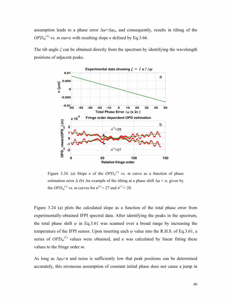
80
assumption leads to a phase error Δψ=Δφ0, and consequently, results in tilting of the
OPDm(1) vs. m curve with resulting slope κ defined by Eq.3.66.
The tilt angle ξ can be obtained directly from the spectrum by identifying the wavelength
positions of adjacent peaks.
Figure 3.24. (a) Slope κ of the OPDm(1) vs. m curve as a function of phase
estimation error Δ (b) An example of the tilting at a phase shift Δφ ≈ π, given by
the OPDm(1) vs. m curves for n(1) = 27 and n(1 )= 28.
Figure 3.24 (a) plots the calculated slope as a function of the total phase error from
experimentally-obtained IFPI spectral data. After identifying the peaks in the spectrum,
the total phase shift ψ in Eq.3.61 was scanned over a broad range by increasing the
temperature of the IFPI sensor. Upon inserting each ψ value into the R.H.S. of Eq.3.61, a
series of OPDm(1) values were obtained, and κ was calculated by linear fitting these
values to the fringe order m.
As long as Δφ0<π and noise is sufficiently low that peak positions can be determined
accurately, this erroneous assumption of constant initial phase does not cause a jump in

81
the demodulated OPD. Under these ideal conditions, the fringe-order shift n(1) in Eq.3.60
can be uniquely determined by minimizing |κ| in Eq.3.66 without hopping to its nearest
integers. However, once Δφ0 reaches π, two adjacent n(1) values generate two possible
solutions for κ with identical absolute values but opposite signs. This degeneracy can
cause a demodulation jump to take place at the point where n(1) jumps to a neighboring
value.
This inherent fringe order estimation ambiguity problem is demonstrated by analyzing
the experimental spectral data near an OPD jump point. Shown in Figure 3.24 (b), when
φ0 is assumed to be constant, it is impossible to distinguish whether the spectrum has
shifted 27 or 28 orders from the reference spectrum. Figure 3.24 (b) illustrates the
relationship between the ambiguity in minimization of the slope κ and calculating the
value of fringe order shift n(1).
Origins of the non-constant phase term
This work investigates two primary causes of variation in spectrogram initial phase:
multimode excitation in the sensor cavity and finite-rate scanning of the interrogation
wavelength. In both cases, contributions to the varying initial phase are represented by
Δφ0.
In the case of optical fiber EFPI sensors, mode-induced variations in initial phase occur
when the wave-front distorted optical wave propagating in free space couples back into
fiber core modes [40]. In IFPI sensors, similar modal coupling issues can occur in the
multi-mode fiber section that makes up the FP cavity, resulting in an OPD-dependent
phase term (see 3.3.1) [59]. The changes of the phase terms of IFPI sensors are generally
much greater than that of the EFPIs during measurement processes, as a result of much
larger OPD changes. The general expression for a spectrogram obtained from an IFPI
sensor is given by Eqs.3.67 and 3.68.
2
22 2 2
1
1 1 effn
Njk OPDjk OPD
n effn
I r e r e
(3.67)
82
1
2
*
0
2A An n
R
dxdy (3.68)
In the above expressions, r denotes the amplitude reflectivity at each interface, and 2
n is
the power coupling coefficient from the fundamental mode of the SMF to the nth mode in
the MMF, the normalized mode profiles of which are represented by A0 and An, and the
integration in Eq.3.68 is performed on the entire fiber cross-section R1. OPDn is the
effective round-trip optical cavity length of the nth mode, which is determined by the
effective refractive index of that mode and the physical cavity length. From Eq.3.67 the
spectrogram is a superposition of N mode vectors representing each mode excited in the
MMF section. The superposition results in a rotating effective vector with amplitude ηeff2
and frequency OPDeff (3.3.1). If τ represents the measurand (strain, temperature, etc.),
the total phase change of the spectrogram when τ changes from τ1 to τ2 can be estimated
by:
2
1
1
ln 2 ceff
n Lk OPD d
(3.69)
In Eq.3.69, nc denotes the refractive index of the MMF core (assuming step-index MMF),
L is the physical length of the cavity, the ∂/∂τ term represents a constant describing the
dependence of the OPD on the parameter to be measured (e.g., if τ represents temperature,
the ∂/∂τ term is the sum of the coefficient of thermal expansion (CTE) and thermo-optic
coefficient (TOC); if τ represents strain, that term equals 1-pe, where pe is the effective
strain-optic constant).
If the spectrogram initial phase φ0 is assumed to be constant throughout the measurement
process, when τ changes from τ1 to τ2, the estimated total phase change is:
2 12 eff effk OPD OPD (3.70)
The additional phase shift is due to multimode excitation is given by the difference
between mode-dependent total phase shift ψ1 and the approximate total phase shift ψ2, the
latter of which assumes constant initial phase:

83
modal 20 1 (3.71)
Equations 3.67~3.71 lead to the conclusion that if there is more than one mode excited in
the MMF cavity, Eq.3.71 results in a non-zero additional phase shift. Furthermore, an
increased proportion of energy carried by higher order modes results in a more significant
shift in initial phase Δφ0.
According to 3.4.2, once this term exceeds π, it results in a jump in the demodulated OPD.
Section 3.4.4 contains simulated and experimental demonstrations of multimode-induced
Δφ0, which show that the multimode nature of the IFPI cavity can produce uncontrolled
phase shifts of 1.2π or greater.
In addition to modal excitation, finite sampling rate of the spectrometer also contributes
to varying initial phase. Assuming the OPD of the sensor changes with speed R
(nm/second) and it takes the data acquisition unit S seconds for a single scan of the probe
wavelength over the spectral range, the OPD change during each scan is given by
ΔOPD = R·S [nm]. The expression for total phase in Eq.3.58 is accordingly modified to:
1 1 0
R Sk OPD k k k
k
(3.72)
where OPD1 and k1 are the OPD and wavenumber at the beginning of each scan, k is
the spectral range of the spectrometer, and φ0 represents the initial phase term generated
by any other effects. The variation in initial phase Δφ0 caused by the sampling can be
calculated from Eq.3.66, while the L.H.S. of Eq.3.66 can be well estimated by ΔOPD/N =
R·S/N where N is the number of fringes in the interference spectrum. The term Δψ in
R.H.S. of Eq.3.66 can be treated as the phase error caused by the finite sampling rate. It is
then straightforward to obtain the initial phase shift Δφ0 due to finite sampling rate using
Eq.3.72, where k0 is the central wavenumber:
2
00
RSk
k
(3.73)
Similar to the case for multimode-induced phase shifts, simulations in 3.4.4 show that
finite-rate sampling can produce an unwanted phase shift of π or greater.
84
3.4.3 Total phase interrogation method
In order to avoid jumps caused by the inherent fringe-order ambiguity problem, the
additional phase shift Δφ0 in Eq.3.60 can no longer be treated as zero. Instead, the
varying phase term 0 0 0 in Eq.3.58 needs to be estimated for each
measurement. The following algorithm is designed specifically to achieve the required
dynamic recalculation of φ0(τ). We begin by re-arranging Eq.3.59 into the following
form, in which the functional dependence on τ is explicitly stated and the fringe order
integers are expressed such that 1
0,1, 2, ..., 1T
Nm N
and m0(τ) is the starting
fringe-order in the spectrum.
01 1
01 1
( ) ( ) ( )
2 ( ) ( )
m N N
N N
OPD k I
m m I
(3.74)
Based on the position of each peak, multiple OPD values can be estimated, as expressed
by the following equation:
1 1 1m m mN N N
OPD c d Y (3.75)
In Eq.3.75, we define the [c] and [d] vectors as: 1 1
2 /m mN Nc m k
,
1 11 /m mN N
d k ,
and an auxiliary phase 0 02Y m . The solution of Eq.3.62 gives the least-square
estimation of the auxiliary phase Y :
1 1
2
0 0
ˆN N
m m mm m
Y C D D
(3.76)
where m m mC c c and m m mD d d , and x denotes the average value of x (averaged over m
fringe orders in a single spectrum). The OPD can then be estimated from the measured
total phase shift based on Eqs.3.75 and 3.76:
ˆ ˆm mOPD c d Y (3.77)
From the auxiliary phase Y , one could also estimate the additional phase term according
to:

85
0ˆ ˆˆ 2 floor / 2Y Y (3.78)
Where the function floor(x) denotes rounding the variable x to the nearest integer less
than or equal to x. In practice, the estimation of 0 and ˆOPD can fluctuate with the same
trend during measurement, which results in unwanted ripples in the measured value of
ˆOPD . This phenomenon is illustrated in the results of experimental testing of the
algorithm. To eliminate this problem, we propose a significant departure from existing
FP sensor interrogation techniques. Instead of monitoring changes in OPD, we define a
new sensor measurement parameter, average total phase , calculated by inserting
measured ˆOPD and 0 into Eq.3.58. represents the total phase at a fixed reference
wavenumber, taken to be the central point in the wavenumber scan range.
0ˆ ˆ( ) ( ) ( )OPD k (3.79)
As proven by the numerical simulations and experimental results, the use of average total
phase as a new measurement parameter allows for dynamic recalculation of initial
phase φ0(τ) while retaining the high measurement resolution of conventional signal
demodulation methods.
3.4.4 Algorithm testing and results
Simulation of multimode-induced phase variation
Computer simulation was performed to verify that the total phase measurement algorithm
can eliminate demodulation jumps when initial phase changes more than π. The
spectrogram of an IFPI sensor was simulated using Eq.3.67 with the step-index optical
fiber parameters outlined in Table 3.6.
A total of 180 spectra, with an SNR of 35dB, were generated and evenly distributed over
a temperature range from 0 to 800oC. As the simulated temperature increased, a phase
shift of about -1.2π was generated due to multimode excitation in the MMF. This phase
shift and OPD change were calculated using the algorithm in 3.4.3 and plotted in Figure
3.25. The blue curve in the figure shows the OPD demodulated using an algorithm which
assumed constant phase. As shown in the figure, when the phase shifts over π, a series of
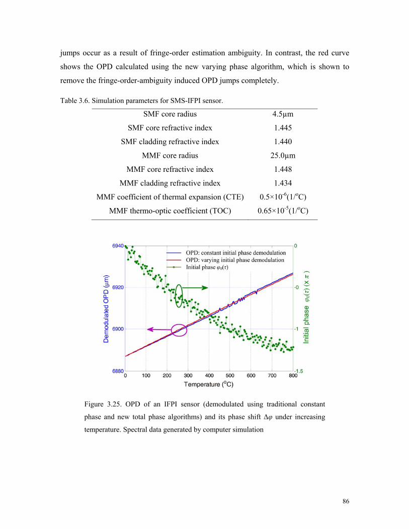
86
jumps occur as a result of fringe-order estimation ambiguity. In contrast, the red curve
shows the OPD calculated using the new varying phase algorithm, which is shown to
remove the fringe-order-ambiguity induced OPD jumps completely.
Table 3.6. Simulation parameters for SMS-IFPI sensor.
SMF core radius 4.5µm
SMF core refractive index 1.445
SMF cladding refractive index 1.440
MMF core radius 25.0µm
MMF core refractive index 1.448
MMF cladding refractive index 1.434
MMF coefficient of thermal expansion (CTE) 0.5×10⁻⁶(1/oC)
MMF thermo-optic coefficient (TOC) 0.65×10⁻⁵(1/oC)
Figure 3.25. OPD of an IFPI sensor (demodulated using traditional constant
phase and new total phase algorithms) and its phase shift Δφ under increasing
temperature. Spectral data generated by computer simulation

87
Figure 3.26. Comparison of simulated, experimental and theoretical variations in
initial phase φ0(τ) due to finite wavelength scan rate S.
Simulation of sampling rate-induced phase variation
In order to demonstrate the effects of finite sampling rate on initial phase, an IFPI sensor
was heated from room temperature to 600oC in 30 minutes, while a total of 180 spectra
were recorded at equal time intervals. The rate of temperature increase varied throughout
the heating process, which led to a non-constant OPD changing rate R. The measured
OPD and additional phase φ0meas of the sensor were estimated at each sampling point
using the algorithm developed in 3.4.3. Next, the rate of OPD change R was estimated
by applying a fifth-order polynomial fit to the measured OPD vs. sample number data.
Using Eq.3.72, the estimated R curve was applied to generate a set of simulated spectra
containing the theoretical dependence of Φ(k) on sampling rate S and OPD change rate R.
This simulated data was then re-processed to calculate its additional phase φ0sim. Figure
3.26 shows the comparison between measured additional phase φ0meas, simulated
additional phase φ0sim, and the theoretical sampling-induced phase shift in Eq.3.73. All
three curves clearly have the same shape, confirming the analytical sampling-induced
phase shift result. A total initial phase shift of slightly less than π is shown to result from
this finite sampling rate phenomenon. The varying total phase algorithm is able to
interrogate the sensor without introducing jumps in the demodulated output.

88
Simulated noise performance
The performance of the total phase algorithm was further evaluated by identifying its
OPD estimation accuracy at different noise levels, as shown in Figure 3.27. The
evaluation method employed was similar to that in [27]. The Mean-Square-Error (MSE)
was evaluated at different cavity lengths and SNR levels by averaging over 1000
measurements at each given condition. An additional phase ranging from 0 to 1.2π was
introduced into the simulated spectra and evenly distributed over the 1000 statistical
sampling points to demonstrate the robustness of the algorithm against phase drifts larger
than π. The corresponding Cramer-Rao bound (see 4.2.2) is also plotted in Figure 3.27 to
show that the varying total phase method can reach the upper theoretical bound of linear
regression-based algorithms even at the presence of a phase shift as large as 1.2π.
Figure 3.27. Performance of the varying total phase algorithm evaluated at
different cavity lengths and SNR levels. MSE errors were calculated based on
1000 sampling points, among which phase shift from 0- 1.2π was evenly
distributed. Each spectrum contains 20000 points spaced over 1520-1570nm.
Experimental evaluation of algorithm
The benefits of the varying total phase algorithm are further demonstrated by the
following two experiments. In the first experiment, an IFPI temperature sensor with
strong multimode excitation was used in order to show the superior performance of the
algorithm in an extreme case, in which large phase shift exists due to the modal behavior
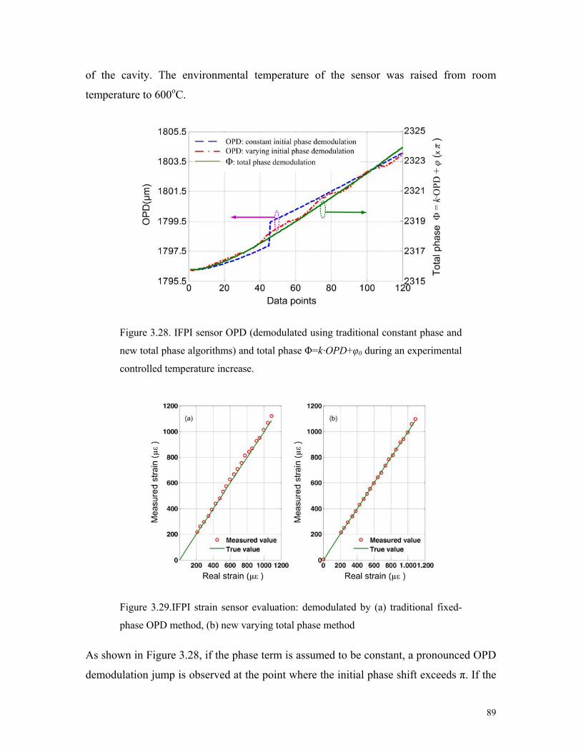
89
of the cavity. The environmental temperature of the sensor was raised from room
temperature to 600oC.
Figure 3.28. IFPI sensor OPD (demodulated using traditional constant phase and
new total phase algorithms) and total phase Φ=k·OPD+φ0 during an experimental
controlled temperature increase.
Figure 3.29.IFPI strain sensor evaluation: demodulated by (a) traditional fixed-
phase OPD method, (b) new varying total phase method
As shown in Figure 3.28, if the phase term is assumed to be constant, a pronounced OPD
demodulation jump is observed at the point where the initial phase shift exceeds π. If the

90
variable initial phase algorithm in Eqs. 3.76, 3.77 is used to demodulate the sensor, the
measured OPD exhibits no demodulation jump. However, the estimated OPD exhibits a
strong, quasi-sinusoidal fluctuation, which is attributed to the heavy modal-excitation in
the cavity as described in 3.3.1 (not to demodulation error).
These periodic fluctuations clearly demonstrate that OPD is not a usable sensing
parameter when initial phase is allowed to vary. Instead, average total phase (Eq. 3.79)
is calculated to quantify changes in the IFPI sensor due to external stimuli. The result is a
demodulated total phase curve that is entirely free from both jumps and sinusoidal
fluctuations (Figure 3.28).
A second experiment was performed to demonstrate the advantage of the total phase
algorithm under varying initial phase due to finite laser scan rate. An IFPI sensor was
stressed by hanging a dead-weight onto the far-end of the fiber link with burst vibration
instabilities caused by swaying of the object. These high-speed fluctuations led to chirp in
the spectra due to the limited speed of the wavelength scanning in the optical detection
and generated an additional phase term according to Eq. 3.73.
As a result, if OPD is used to characterize the sensor, the strain calibration curve (strain
versus demodulated OPD) in Figure 3.29 (a) is full of small fluctuations and suffers from
poor repeatability. This is reflected by the large measurement error (RMSE = 19.9µε)
obtained using the traditional OPD algorithm. Instead, if the total phase is used to
characterize the same fluctuating IFPI data, it results in much better repeatability and
measurement accuracy (RMSE = 5.4 µε) as shown in Figure 3.29 (b).
3.5 Conclusion
In this chapter the reflection mode SMS fiber structure employing the GI-MMF (SMS-
IFPI) was studied. Splicing reflectivity, IFPI refocusing, and the additional phase in the
sensor spectrum were analyzed and discussed. An analytical expression for the SMS-IFPI
spectrum, with the reflectivity dictated by the fiber axial index profile was deduced. The
model provided a means by which the physical background of the cavity reflection was
clearly understood. The IFPI cavity refocusing effect was studied by a ray matrix

91
approach and fiber modal analysis. The multiplexing capacity of the SMS-IFPI fiber
sensors was dramatically increased by promoting refocusing of the propagating light.
Wave-front distortion in the MMF section of a SMS-IFPI sensor is a direct result of the
multi-modal nature of the cavity. Similar to EFPI fiber sensors, the wave-front distortion
generates an additional phase term in the interference spectrogram of the sensor. The total
phase in the spectrogram is modeled by a rotating effective vector. The OPD
demodulation process mathematically is the estimation of the rotational speed of the
effective vector with respect to wavenumber by looking at the interference spectrum, but
the information obtained herein can be misleading to some extent. Hence the error in this
first-step estimation amounts to an additional phase shift in the formula used to calculate
the total phase. It is predicted that in a real application, if the OPD change is small in a
measurement, the change of the additional phase term will not be significant and high
measurement accuracy can still be obtained; however, for applications where OPD
changes are large, it is possible that the phase term will change very rapidly and accurate
OPD decoding will be difficult.
The resultant non-constant phase term in the fiber sensor spectrogram plays an important
role in sensor signal demodulation. When a phase shift of π occurs, an ambiguity arises in
fringe-order estimation, generating an abrupt jump in the OPD calculated by traditional
constant-phase algorithms. These phenomena can cause the resulting measurement to
suffer from poor accuracy, even in sensors with high signal-to-noise ratio.
To avoid such jumps, we present a demodulation algorithm based on two key innovations:
continuous calculation of a time-varying initial phase, and use of total phase as a
measurement parameter instead of OPD. The varying total phase algorithm is shown to
have high resolution and to eliminate spurious jumps caused by both multimode
excitation and slow wavelength scanning rate. As long as the additional phase shift stays
within 2π, no ambiguity exists in the total phase.

92
Chapter 4 WLI-Based Signal Processing
4.1 Introduction
In the previous chapters, both EFPIs and IFPIs have been theoretically studied. In their
applications, the change of the optical path difference (OPD), defined as twice the
product of the cavity length and the refractive index of the cavity material, is almost
linearly related to the physical parameters being measured; as a result, the key of signal
processing is to make accurate measurement of the OPD. The reflection spectrum of the
FP sensor is expressed as [93]
2
1 cos2
1 2 cosI R
R R
(4.1)
where R is the reflectance of the cavity mirrors (assume identical reflectivity) and Φ
denotes the total phase defined through Φ = kOPD, where k is the wavenumber in
vacuum. In the regime of “low-finesse”, the reflectances of the cavity mirrors are low and
multi-reflection is neglected. Such low-finesse FP sensors are more cost-effective, and
most importantly, they exhibit outstanding robustness in harsh environments [14]. For
such sensors Eq. 4.1 is reduced to
I(Φ) = 2R[1-cos(Φ)] (4.2)
which appears sinusoidal with respect to Φ, and Φ is linear with both OPD and k. In
fringe counting mode, a fixed-wavelength laser (or several of them) is injected into the
sensor and the reflected power is modified sinusoidally with the OPD (when k is fixed)
[22]. Unfortunately as the output is inherently periodic, it provides only relative OPD
measurement. Absolute measurement is apparently more desirable and can be achieved
using white-light interferometry (WLI) in which a broad-band optical source is used.
With WLI, the OPD is measured either by matching the cavity length of a reference
interferometer [11] or by direct analysis of the reflected spectrum, the latter is the subject
of this chapter.

93
Figure 4.1. Schematic of the fiber optic WLI -FP sensing system.
The schematic of the WLI sensing system is depicted in Figure 4.1. The spectrum
interrogation unit comprises of a broadband source and a spectrometer (or a swept-laser
spectrometer) which records the reflection spectrum of the FP sensor and sends the data
to a processing unit (computer) for demodulation. The spectrum is sinusoidal with
wavenumber k according to Eq. 4.2. A variety of demodulation methods have been
developed to calculate the OPD directly from the spectrum, and they can be classified
into two categories.
The first type is denoted as TYPE I (direct frequency estimation), which relies on the fact
that the spectrum is a harmonic function of k, with OPD being the frequency. Estimating
the frequency can be achieved by using periodogram (i.e., by Fourier Transform, FT) or
phase linear regression. Periodogram is mostly adopted in which the frequency is
estimated by tracking the peak position in the FT of the spectrum [37, 45, 94-96], this
method is especially powerful for demodulation of multiplexed sensors. An alternative
TYPE I approach relies on Φ = OPDk where multiple Φ and k values are obtained from
the spectrogram, consequently calculation of OPD is converted to frequency estimation
by linear regression. A simple but popular version uses only two points, which usually
employs peaks, valleys or zero-crossing points [97-99]. This method offers low
resolution and works better for situations where only few peaks exist in the spectrum. If
more peaks are available, it is straightforward to use more points to maximize
information utilization. In such cases, multiple peak/valley points [42, 100] or the whole
spectral data [41, 101] are used for the linear regression.
The second type of algorithm, named TYPE II (total phase), also relies on the
relationship Φ = OPDk. In a simple version, the spectral position k of one peak is

94
accurately determined, and the OPD is obtained by Φ/k where the value Φ of the peak is
known if the corresponding fringe order is found. Without the knowledge of the fringe
order there is an 2π ambiguity in Φ [102]. In order to enable absolute measurement, an
improved algorithm estimates the fringe order in the first step by FT or linear regression
and subsequently determines the OPD by tracking one peak [39, 103]. This strategy was
extended further to utilize the whole spectrum [27]. Apart from estimating only the
frequency component in the spectrograph as in TYPE I methods, this approach seeks to
estimate the total phase Φ at given spectral points k (or vice versa). Similar task was also
accomplished by iterative curve fitting [40, 46, 47].
Despite the success of these developed methods, problems still exist. It is widely
accepted (and will be demonstrated later) that the TYPE II approach (total phase) is more
accurate than TYPE I (frequency estimation) in calculating the OPD. Unfortunately
because the total phase is periodic in nature, a 2π ambiguity may occur during
implementation which leads to abrupt discontinuity (or “jumps”) in the demodulated
OPD [27, 40, 46, 47] (it should be noted that jumps only exist in TYPE II estimations).
To date, the cause of the jump is still not thoroughly understood, and consequently
eliminating the jump is still not promising. Moreover, a theoretical framework is missing
within which the performance of the different algorithms can be evaluated and compared.
Due to these reasons, it is reasonable to conclude that the practicality and potentiality of
the WLI algorithms are still not fully exploited.
This chapter constructs a set of theories and criteria upon which the performance of the
algorithms can be evaluated, and the cause of the jump problem is completely explained
(section 4.2). We emphasize the role of an additional phase term which acts as a “hidden
killer” to cause the jumps, and propose a more appropriate definition of the total phase
with the hope of maximizing noise reduction while maintaining minimum jump risk. In
4.3, the theories will be verified and discussed. Three WLI algorithms will be compared
and their pros and cons will be concluded. The physical cause of the additional phase will
be further expounded and a solution to minimize the jump occurrence will be
demonstrated.

95
4.2 Theory
4.2.1 Background
In deriving Eq. 4.1, plane wave with normal incidence (parallel to cavity axis) is assumed.
In real application, the beam inside the cavity is diffraction limited and its divergence
gives rise to a roundtrip power coupling factor ν and accordingly Eq. 4.1 is modified to
2
2 2
1 2 cos
1 2 cosI R
R R
(4.3)
with ν<1. I(Φ) is periodic with Φ and can be subsequently expressed by a Fourier series
as
01
cosnn
I a a n
(4.4)
with Fourier coefficients an (the sine terms are absent due to symmetry). It is shown that
the intensity ratio between adjacent harmonics is (for n > 0):
1n na a R (4.5)
which dictates that higher harmonics are orders of magnitude weaker than the
fundamental component and can be neglected. As a result we are left with a pure
sinusoidal signal which, after normalization appears to be
2
21 cos
1normI k OPD
(4.6)
The influence of beam divergence is to reduce the signal strength by a factor of 2ν/(1+ν2)
which is usually referred to as the fringe visibility.
The above discussion only takes into account the loss generated by beam divergence. In
fact, divergence also distorts the phase front of the beam, which introduces another phase
term φ0 in the total phase Φ when coupled back into the lead fiber [40]. Eq. 4.6 is finally
written in the following form (where φ0 + π is combined into φ0):

96
02
21 cos
1normI k OPD
(4.7)
which best describes the spectrum of a real low-finesse FP sensor. The TYPE I
(frequency estimation) approaches calculate OPD directly from the density of the fringes,
thus the phase term φ0 is ignored. On the contrary, this term needs to be considered in the
TYPE II approach due to its direct contribution to the value of the total phase, and is
usually treated as a constant and pre-calibrated [27, 39]. Nevertheless, this treatment is in
most cases not suitable and will result in the demodulation jumps, as will be discussed
later.
Most spectrometers provide spectral position readings in unit of wavelength (λ), which
result in uneven distribution of k (i.e., k = 2π/λ). It is recommended that the spectrum to
be interpolated to yield equal sampling interval in k to take full advantage of standard
signal processing techniques. The interpolation error is minimized if “cubic spline”
interpolation is used and the associated interpolation error shows negligible influence on
the final estimation quality, as will be demonstrated in 4.3.2.
We conclude that the OPD estimation problem is now converted to standard harmonic
analysis. Before continuing to the theories, the scope of the subject matter needs to be
further clarified. The signal is a discrete, real-valued sequence, with unknown parameters
OPD (frequency) and φ0 (phase) to be estimated. Because the data is real-valued, we
define the normalized frequency by ωn = ω/(2ωs) where ωs is the angular sampling
frequency, thus
n OPD k (4.8)
where Δk denotes the spectral sampling interval. As can be easily verified, for real
systems Eq. 4.8 always yields a number <0.1, which suggests that the signal have
“moderately low” frequency. The phrase “moderately low” is picked to distinguish from
“extremely low”, in which the FT peak in the periodogram is nearly indistinguishable
from the direct current (DC) that standard frequency estimation methods (such as the
ones to be introduced in 4.3.1) tend to generate large errors. In such cases, the method in
[39] is suggested. If the FT peaks are clearly resolvable in the Fourier domain, classical

97
non-parametric periodgram yields the best performance (i.e., the maximum likelihood
estimator) [28], this condition is satisfied for most cases, and is the subject of this chapter.
More specifically, this work is confined to single harmonic analysis. For multi-tone
analysis usually a filter is used to select the corresponding frequency component,
however the problem is complicated by issues such as cross-talk among different
channels and the lower bounds of the estimators need to be modified [28]. If multiple
harmonic components closely co-exist with deteriorated resolution on the periodogram,
parametric methods can be applied [30]. In some applications, the signal is amplitude-
modulated by an envelope stemming from the source spectrum. The envelope can be
removed by pre-calibrating the source spectrum or by an interpolation process [27, 103].
In sum, after the removal of the envelope and the DC component, the signal is expressed
as
0cosn n nI A OPD k W (4.9)
where A is the amplitude and kn is the fixed sampling wavenumber and In is the measured
intensity at kn, which is contaminated by zero-mean white Gaussian noise Wn with power
σ2=var[Wn] (var[] denotes the variance). The quantities in Eq. 4.9 are all real-valued
and n = 1, 2, …N (N is the length of the data). OPD and φ0 will be the parameters to be
estimated, their corresponding estimation values are denoted as ˆOPD and 0 respectively.
The signal to noise ratio (SNR) is defined as S = A2/(2σ2) [104]. The beginning
wavenumber is defined as k0 and subsequently kn = k0 + (n-1)Δk, and we define a central
wavenumber
kc = (k1+kN)/2 ≈ k0 + N Δk/2 (4.10)
which is heavily used throughout the rest of the chapter. Two WLI systems will be
applied for simulation and experimental demonstration of the theories. Their system
parameters are listed in Table 4.1.

98
Table 4.1. List of key parameters of the WLI systems used in the research.
System number
Source Spectrometer Wavelength range (nm)
N k0
(μm-1) Δk
(m-1) Remarks
1 LED OceanOptics Inc.USB2000
715.88-980.64
2048 6.4072 1157.6 Multimode fiber based
2
Micron Optics Inc., Swept laser spectrometer with built-in source, Si-720
1520-1570 20000 4.0020 6.5826 Single-mode fiber based
4.2.2 The theories
Cause of the jump (I): the constant φ0 assumption
For the TYPE II (total phase) methods, if φ0 is assumed to be a constant, the jump
problem becomes inherent when in fact φ0 changes during the measurement and the
change exceeds π. A detailed analysis of this phenomenon is found in 3.4.2 and Ref.[60].
This can be intuitively understood as follows. While φ0 shifts, as long as the drift is less
than π, the algorithm can find a nearest fringe order (N0) by a rounding process [39].
However, when the shift is beyond π, the nearest fringe order suddenly moves to N0 1,
and the jump occurs. As a result, assumption of a constant φ0 should be avoided to
prevent jumps.
Total phase estimation with varying φ0
As stated in the previous subsection, when applying the TYPE II approach (to calculate
the total phase), φ0 cannot be treated as constant. Instead, it should be estimated along
with the OPD, and the total phase can be estimated by [60]
0ˆˆ ˆck OPD (4.11)
where ˆOPD and 0 are estimated by the TYPE I algorithm and subsequently an
estimation of OPD with better resolution is given by:
ˆ ˆtot cOPD k (4.12)
The subscript “tot” denotes TYPE II OPD estimation by total phase. A major advantage
of TYPE II estimation is its superior noise reduction capability. In 4.2.2 and 4.3.5 the
99
noise reduction mechanism of the TYPE II approach will be analyzed. Moreover, using
total phase also benefits from a reduction of bias and demodulation nonlinearity, as will
be discussed in 4.3.3, 4.3.5.
Using Eq.4.11, the prerequisite of constant φ0 is removed. Typically, φ0 depends on OPD
in a deterministic way and can be calibrated within the measurement range (e.g. by
polynomial fitting φ0 = P(OPD)). In real practice, one needs to estimate ˆOPD and 0 in
the first step. Similar to Φ, φ0 is also a phase term and is consequently subject to 2π
ambiguity. If φ0 is pre-calibrated (meaning the relationship of φ0 = P(OPD) is found), one
can calculate the expectation value of φ0 at the given ˆOPD as 0 = P( ˆOPD ), and set a
2π range [ 0 - π, 0 + π] to determine 0 . As will be shown in 4.3.5, this technique can
reduce the probability of jump by several orders of magnitude.
The lower bounds
For an estimator its performance can be evaluated by the mean square error (MSE)
2 2ˆ ˆ ˆ[( ) ] [ ] [ ] E var bias (4.13)
where E denotes average, and is the estimated value of the parameter θ. In general the
estimator is assumed to be unbiased and the MSE reduces to the variance of the estimator.
However unbiasedness is not a straightforward assumption and will be discussed in detail
in 4.3.3. In any circumstances, the variance of the estimator cannot be arbitrarily small,
the lower bound of which is defined by the Cramér-Rao bound (CRB). Here, without
proof, the CRBs for the frequency and phase estimations in WLI are given, the
derivations can be found in [105]. Define P = N(N-1)/2, Q = N(N-1)(2N-1)/6, n0 = k0/Δk,
and Y = n02N + 2n0P+Q,
The CRB of OPD estimation with unknown φ0 is (OPD of TYPE I):
2 2
12ˆ[ ]1
OPDS k N N
var (4.14)
The CRB of OPD estimation with known φ0 is (this is an approximation of the CRB of
TYPE II OPD. See 4.3.5):

100
2
1ˆ[ ]OPDS k Y
var (4.15)
The CRB of φ0 estimation with unknown OPD is (φ0 of TYPE I):
0 2 2
12ˆ[ ]
1
Y
S N N
var (4.16)
The CRB of φ0 estimation with known OPD is (Φ of TYPE II):
0
1ˆ[ ]
S N
var (4.17)
For WLI systems, both OPD and φ0 are unknown. Eq. 4.14 defines the lower bound of
the OPD estimation variance for the TYPE I algorithms (“frequency estimation”), the
lower bound of phase estimation variance of TYPE I methods is given by Eq. 4.16. Eq.
4.17 is the CRB of Φ estimation (total phase of TYPE II, Eq. 4.11), and accordingly the
TYPE II OPD estimation ( ˆtotOPD ) has a variance limit of
2
1ˆ[ ]totc
OPDS N k
var (4.18)
To demonstrate that Eq. 4.17 is the CRB of , we take the variance on both sides of Eq.
4.11, and notice that when the frequency (OPD) is known, the variances of and 0
coincides, which sets the lower bound of the total phase estimation. A more detailed
explanation of the noise reduction mechanism of the total phase approach will be given in
4.3.5. The benefit of using total phase is clear when Eq. 4.18 and Eq.4.14 are compared.
The root mean square (RMS) error of the direct frequency estimation is much larger than
the total phase based OPD estimation by a factor of (by taking the square root of
(Eq.4.14)/(Eq.4.18))
0 12 3
2
nG
N
(4.19)

101
For WLI System I, it is calculated that G ≈ 11.09 and for WLI System II, G ≈ 107.04.
This predicts that the OPD estimation resolution using total phase is approximately 10dB
and 20dB better than the direct frequency estimation, for system I and II respectively.
More benefits of using total phase will be further discussed in section 4.3.5. In general, if
high resolution is required, total phase demodulation is recommended. However, one
major drawback of the approach is the potential of the demodulation jumps.
Cause of the jump (II): estimation noise of φ0
The probability density function (PDF) of 0 is a Gaussian with mean φ0 and variance
2p (the lower bound of the variance is defined by Eq. 16) and is expressed as
2
0 020 0 2
ˆ1ˆ ; , exp
22p
pp
f
(4.20)
As discussed in 4.2.2, a 2π range is assigned to φ0 in order to unambiguously determine
its value. A jump event will occur if 0 falls out of the assigned range, this would lead to
addition or subtraction of multiple 2π’s in order to force 0 back to the given range. The
probability of jump is minimized if the range is centered at φ0, where the probability is
defined by the following inequity:
20 0 0ˆ ˆ2 ; 2 ; ,jump pP F f f d
(4.21)
where F denotes the cumulative distribution function. It should be noted that in principle
the jump cannot be eliminated (value of Eq.4.21 is always >0), however it can approach
zero if σp is small and the 2π range is appropriately selected. The jump probability
minimizes when the estimator reaches the CRB and the 2π range is centered at φ0. One
can thus estimate the jump probability by Eqs. 4.16 and 4.21. The probability escalates
rapidly if σp is large and/or the range is not centered at φ0, we will illustrate this situation
in more detail in 4.3.5.

102
4.3 Discussion
4.3.1 WLI algorithms
The periodogram (FFT method)
The maximum likelihood estimator of single harmonic is the periodogram which can be
regarded as the best algorithm [28, 105]. However, this method has been considered to
yield poor accuracy when applied in WLI. The reasons for this belief are: 1) periodogram
was used as a TYPE I estimator in the past, i.e., only ˆOPD is estimated. As a result of the
discussion in 4.2.2, compared with the TYPE II approaches, the resolution of
periodogram is worse; 2) the implementation of the algorithm is not optimized.
Because the signal is real, its FT is symmetric about zero and only N/2 data points are
effective in the periodogram. This basically dictates the normalized frequency resolution
to be limited to 2/N. To improve the resolution, zero padding is widely adopted to
increase N [37]. Taking derivative of Eq. 4.8 on both sides, and denoting the frequency
resolution as dωn = 2/N, it is found that in order to resolve a frequency difference of
δOPD, the number of points needed is
2cN
OPD
(4.22)
in which λc is the central wavelength and Δλ is the wavelength interval of the
spectrometer. To achieve resolution of δOPD = 1Å, for WLI System I, N = 7.4 x 10⁷ and
for WLI System II, N = 9.6 x 10⁹. The required data size will lead to unrealistic
computational load and result in extremely low efficiency. To improve its efficiency, it is
recommended that following a rough estimation of the FT peak position with relatively
short N, the normalized frequency in Eq. 4.8 is further determined by the Newton-
Raphson method to maximize [28, 105]
1
0
expN
n n nn
A I i n
(4.23)
and the estimations of OPD and φ0 are obtained by
ˆ ˆnOPD k (4.24)
103
0 0ˆˆ ˆarg exp niOPD k A (4.25)
This method is expected to yield the maximum-likelihood estimation to reach the CRB. It
is abbreviated as FFT method and will be discussed further in the following subsections.
Linear regression (LR method) and peak tracking (PT method)
In the linear regression method, Φ of all the data points are calculated by solving the
angle of the analytical signal, followed by a linear fitting to their corresponding spectral
positions kn, details of the method can be found in [27]. Eq. 4.13 in [27] is used to
estimate the OPD and φ0. This method is abbreviated as LR.
Instead of using all the spectral points for linear regression, the peak tracking method
uses only the peak positions in the spectrum. Corresponding details can be found in 3.4.3
([60]), and Eqs. 3.77 and 3.78 in 3.4.3 are used to determine the OPD and φ0. This
method is abbreviated as PT. At first glance the accuracy of PT should be lower than LR
because only a small portion of the spectral data (only the peak points) are used; however
this is not true because actually all the points contribute to the determination of the peak
positions.
For the LR and PT methods, it is important to use a band-pass filter to clean the signal in
advance to increase the breakdown threshold (which is defined as a SNR value beyond
which the error of the estimator abruptly becomes significantly larger than the CRB) [27].
It is found that an effective order of the filter is Nf = N/10. If Nf is too small, the noise
reduction is not sufficiently effective; on the contrary, if Nf is too large, the effective
length of the data is sacrificed to an extent that the CRB is apparently lifted. It is also
important to shift the filtered data back Nf/2 points to compensate the filtering delay,
otherwise a large phase bias would occur.
4.3.2 Evaluation of the algorithms
The algorithms in 4.3.1 were evaluated by comparison with the corresponding CRBs
using computer simulation. In the simulation, an FP cavity with OPD = 200μm was
assumed, and the parameters of WLI System I was used. White Gaussian noise was
added to the sensor spectrum according to the required SNR. At each SNR level, one

104
thousand sets of spectral data were generated, and the variances of the FFT, LR and PT
methods were calculated for both TYPE I and TYPE II (by using Eqs.4.11,4.12)
estimations. Plotted together are the corresponding CRBs.
Figure 4.2. Performance evaluation of the FFT, LR and PT methods, plotted
together in both figures are the standard deviation of both the TYPE I and TYPE
II estimators. a: OPD estimation and b: φ0 estimation. The CRBs for the
corresponding variances are co-plotted. Insets are zoomed-in views of the curves,
which provide better visibility of the algorithms’ performances.

105
On the figure of OPD estimation, the CRB for frequency estimation with known phase
was plotted, which is sufficiently accurate as the CRB for TYPE II OPD estimator (see
4.3.5). Because the estimators were assumed to be unbiased, the simulation used their
standard deviation as the RMS error. The discussion on estimator bias is given in 4.3.3.
As demonstrated by Figure 4.2, all three algorithms approach the CRBs nicely. It should
be noted that the input spectrum was evenly-sampled in wavelength. Reaching the CRB
demonstrated the effectiveness of the interpolation process that evenly sampled the
spectrum in wavenumber. The FFT method, as expected, shows the best performance,
whereas the LR and PT methods demonstrate nearly identical performances. The
threshold of the LR and PT methods take place at SNR~-5dB, the FFT approach shows a
lower threshold below -10dB, which suggests better immunity to noise. Reaching the
CRB is a manifestation of the performance optimization. In other words, once an
algorithm approaches the CRB, it reaches the ultimate limit given the amount of
information. Any other WLI algorithms can be evaluated against the CRB under the same
framework.
4.3.3 Comparison of the algorithms
Estimator bias
In the previous discussions, the estimators are assumed to be unbiased [105], which is in
fact not true for the current situation. The reason is closely related to the properties of the
WLI signal. As noted in 4.2.1, the harmonic under analysis is real-valued and bears very
low frequency. Unlike complex-valued signal (analytic signal), the real signal is
symmetric about zero on the Fourier domain. When the harmonic frequency is low, the
positive and negative peaks associated with the harmonic are very close to each other. As
the sequence is of finite length, spectral leakage will take place [104, 106], manifesting as
side lobes near the FT peaks. The side lobes of the negative peak interfere with the
positive peak and slightly change its spectral position. The modification is small but a
noticeable bias is incurred when high accuracy is required.

106
Figure 4.3. Absolute value of OPD bias versus cavity length plotted for TYPE I
LR, FFT and windowed FFT (Blackmanharris) estimators. The result for TYPE
II estimator using FFT (Blackmanharris) is co-plotted, which demonstrates
superior bias suppression.
Windows can be applied to the data to effectively suppress the intensity of the side lobes.
The performances of different windows are compared by computer simulation, in which
the cavity length of the FP sensor was continuously swept from 3μm to 100 μm, with the
cavity refractive index set to unity. During the simulation no noise was added, and the
WLI System I parameter was used in the study. The TYPE I OPD estimated using LR,
FFT and windowed FFT (with Blackmanharris window) are obtained and the bias of each
estimator at the given cavity length was found by comparing with the true value. The
results are shown in Figure 4.3. A common feature shown is the tendency toward short
cavity, where the influence of spectral leakage surges rapidly for all the estimators,
resulting in increased bias. Another feature is the bias’s pattern that oscillates with the
cavity length, which is apparently a signature of the side lobes. For TYPE I estimation,
FFT and LR show unsatisfactorily large bias. Even at cavity length of 100μm, both show
a maximum bias of ~10 nm. The oscillatory pattern will promote demodulation
nonlinearity. Demonstrated is the effectiveness of windowing to suppress the bias. As
shown by the dotted curve, application of Blackmanharris window leads to a bias

107
suppression ratio over 30dB, the maximum bias was reduced below 10pm for cavity
length from 10 to 100μm.
During simulation, φ0 in the spectrum was set to zero, as a result the TYPE II OPD
estimator (Eqs. 4.11, 4.12) becomes unbiased (otherwise TYPE II estimator has an
constant bias, which will be discussed in 4.3.5). It is found that the TYPE II estimator
shows superior bias reduction, which suppressed the bias further for another ~15dB. The
maximum bias for cavity length ranging from 10 to 100μm was uniformly below 1pm,
which is of significant importance for high-accuracy applications.
Comparison of the algorithms
In 4.3.2 the performances of the algorithms are evaluated by comparing with the CRBs.
In the previous demonstration only the variance is considered. According to Eq. 4.13, the
MSE also includes a bias term; as is discussed in the preceding section, the estimators are
generally biased which calls for re-examination of their performances. Comparison was
made among FFT, LR and windowed FFT (with Blackmanharris window), for both
TYPE I and TYPE II estimations by computer simulation, the simulation assumes WLI
system I parameters. In order to make the influence of bias more visible, the OPD of the
simulated spectrum was shortened to 60μm. At each SNR level, the RMS error was
calculated based on comparison of the estimated and true OPD values with 1000
observations. The results are plotted in Figure 4.4. The RMS errors of the TYPE I LR and
FFT estimators diverge significantly from the CRB for SNR > 10dB, which is attributed
to a big bias. The curve corresponding to windowed FFT in the TYPE I group follows the
CRB nicely in the whole SNR range except for a uniform ~3dB degradation. This is
attributed to the larger equivalent noise bandwidth associated with the window used [106].
For TYPE II estimators, FFT without windowing shows the worst performance (diverge
significantly from CRB starting at SNR ~ 10dB). For the TYPE II LR estimator,
significant divergence from CRB happens above SNR ~ 25dB. The performance of the
windowed FFT is consistent in the complete SNR range. According to the simulation, for
TYPE I estimation, windowed FFT is preferred if SNR is over 20 dB. For TYPE II
estimation, for SNR > 30dB, windowed FFT has the best performance, otherwise LR
method is sufficient. For applications with high SNR and requiring high accuracy, TYPE

108
II windowed FFT is the best choice. The simulation predicts that for WLI System I, at
SNR =40 dB the RMS estimation error is ~50pm if TYPE II FFT with Blackmanharris
window is used.
Figure 4.4. Performance comparison of the LR, FFT and windowed FFT
(Blackmanharris). The RMS error includes the contributions from both the
estimator variance and bias. The windowed FFT for both TYPE I and TYPE II
estimations manifests superior performance in bias reduction, at the expense of a
~3dB increase in the RMS error.
The computation complexity of the FFT, PT, and LR estimators were compared in terms
of computation time. The time was measured by averaging over 1000 executions and as a
function of data length (N), the result is plotted in Figure 4.5. The investigated algorithms
show that the computation time linearly increases with N. The LR and PT methods have
nearly identical complexity, while the complexity for the FFT method is significantly
higher. The calculated complexity can be influenced by a number of factors such as CPU
speed and programming skills. However the significantly higher complexity of the FFT
estimator is as expected [107].

109
Figure 4.5. Measured computation complexity in terms of execution time, plotted
as a function of data length (N). The FFT, PT and LR methods are compared to
demonstrate linear relationship with N. The complexity of FFT is the highest
while the complexities of PT and LR are almost identical.
4.3.4 OPD-dependent additional phase
We discussed in 4.2.2 that the “constant φ0” assumption will intrinsically lead to
demodulation jumps if TYPE II estimation is made. We concluded from numerous
experimental observations that the φ0 term for both EFPI and IFPI is, in general,
dependent on OPD, and more importantly, is usually a function of OPD. Being a function
of OPD makes the φ0 calibratable, which is the key to reducing the probability of jumps
as will be discussed in 4.3.5. In this subsection some major causes of the OPD-
dependent φ0 will be introduced; nevertheless, factors not included in this subsection may
also cause a changing φ0.
Phase front distortion
The φ0 change due to phase front distortion is an inherent property of the FP cavity. In
other words, unlike other factors, it is a “built-in” signature of the cavity and is
unremovable by any hardware and/or software. At the cavity interface, the optical beam
will be diffracted from a fiber mode into either a free-space mode (for EFPI) or other
fiber modes (for IFPI). During propagation, the phase front of the cavity mode will
110
become distorted, and a non-zero phase term will be generated when the phase-front-
distorted beam is recoupled back into the lead-in fiber. Intuitively, the greater the
distortion is, the larger the phase term would be; as the distortion is OPD-dependent, so is
the induced phase. For EFPI, detailed analysis can be found in [40, 52, 108], and the case
for IFPI was studied in [59]. In general, for EFPI, the phase term caused by phase front
distortion is small and changes moderately with OPD; for IFPI, due to multi-mode
excitation, this term could be large and change more rapidly.
Material dispersion
If the FP cavity is filled by a material with chromatic dispersion (i.e., not air), and while
the spectral bandwidth of the spectrometer is large (e.g., WLI System I), material
dispersion can cause a “chirp” in the spectrum which finally amounts to a spurious phase
term. The material dispersion is described by the Sellmeier model, the coefficients of the
model are all temperature-dependent. For a temperature sensor, changing the temperature
subsequently changes the OPD, while the Sellmeier coefficients simultaneously vary to
cause a changing φ0. This was simulated using the parameters of the WLI System I and a
silica wafer with initial thickness of 70μm. Dispersion of the wafer was modeled by the
temperature-dependent Sellmeier model with parameters from [67]. During the
simulation, temperature was increased from 20oC to 1300oC, and the linear coefficient of
thermal expansion (CTE) was set to 8.5x10⁻⁶. The φ0 term was calculated using
Blackmanharris windowed FFT and plotted as the solid line in Figure 4.6. The agreement
of the simulation result with experiment will be given later in 4.3.5.
Fixed-pattern noise (FPN)
A pixel-sensor (such as a CCD) usually bears fixed-pattern noise due to uneven pixel-to-
pixel sensitivity [109]. Some spectrometers (such as the spectrometer used in WLI
system I) are built with such devices. Typically the FPN is small enough for accurate
spectral analysis, however for sensitive OPD measurement, the influence from the FPN
can be noticeable. The OPD-dependent phase term φ0 can be understood as follows. The
spectrum of the FP sensor with the FPN is written as (with time-dependent noise
excluded)
0cosn n nI A OPD k W (4.26)

111
where nW represents the FPN. The Fourier domain spectrum is thus expressed as
k k n k kI I S w FFT (4.27)
where Sk is the FT of the harmonic signal and kw is the FT of the FPN. A major
difference between the FPN and normal noise is that kw is fixed for each Fourier bin.
Figure 4.6. Computer-simulated phase term φ0 caused by material dispersion
(solid) and fixed-pattern noise (dashed). The dispersion of a 70μm-thick silica
wafer was modeled by the temperature-dependent Sellmeier model. WLI System
I, together with Blackmanharris windowed FFT was used for signal
demodulation. For the simulation of fixed-pattern noise, the applied white
Gaussian noise yields a SNR = 12 dB.
When OPD changes, the FT peak position scans continuously, and the interference from
w is dependent on the peak position, thus the OPD estimation error becomes OPD-
dependent. This OPD error is finally translated to a phase error via Eq. 4.25. The FPN
induced phase shift always shows up with an oscillating pattern (with respect to OPD)
with a period roughly equal to λc (the central wavelength). This can be easily understood
by recalling that after the OPD shifts λc, the spectrum nearly recovers, and the influence
by the FPN will consequently repeat. The FPN-induced phase was simulated by adding a

112
fixed white Gaussian noise to the spectrum acquired by WLI system I, which resulted in
an equivalent SNR = 12 dB. This noise was added upon the spectra which are previously
used to simulate and plot the dispersion-related phase (Figure 4.6, solid curve), and the
final results are shown on the same figure as the dashed curve. The simulated influence
indeed shows up as an OPD-dependent oscillatory phase term.
Finite sampling rate (FSR)
If the spectrometer has a finite sampling rate (FSR) across the full spectral range (e.g.,
WLI System II, the laser scanning rate is 5 Hz), the FSR will couple with the OPD
changing rate to generate an additional phase. The added phase can be expressed as [60]
2
0c
s
kdOPD
dt f N k
(4.28)
where fs denotes the scanning frequency and the derivative term represents the OPD
changing rate. Among all the factors that induce the OPD-dependent φ0, this FSR-
induced phase is the most difficult to be removed, because it depends on the
instantaneous OPD changing rate, and thus cannot be pre-calibrated.
4.3.5 More on total phase
The noise reduction mechanism of TYPE II estimations
In 4.2.2, we have shown the noise reduction gain (defined as the ratio between the RMS
errors of TYPE I and TYPE II estimations) in Eq. 4.17 and a simple proof of the
statement is given in 4.2.2. In this section we will explain more on the noise reduction
mechanism of the TYPE II approaches.
Taking the variance on both sides of Eq. 4.18, we get
20 0
ˆ ˆˆ ˆ ˆ[ ] [ ] 2 [ , ] [ ]c ck OPD k OPD var var cov var (4.29)
where cov[] denotes the covariance. The values of the terms on the right-hand-side of
Eq. 4.29 can be obtained from the components of the inversed Fisher information matrix,
and correspondingly labeled as J(i,j) (i,j = 1,2). The values of ˆ[ ]OPDvar =J(11) and

113
0ˆ[ ]var =J(22) are defined in Eqs. 4.14 and 4.16, respectively. The value of 0ˆ ˆ[ , ]OPD cov
is determined by the anti-diagonal elements J(1,2) = J(2,1) which can be calculated as:
0(1,2) (2,1)
2
6 2 1
1
n NJ J
S k N N
(30)
The value is negative and sets the lower limit of the covariance in the sense that |cov[]|
|J(1,2)|. To estimate the variance of we insert Eqs. 4.14, 4.16 and 4.30 into Eq. 4.29, and
get
2 2
0
2 2 2
12 12 2 1 12ˆ[ ]1
c ck N k k n N N k Y
S k N N
var (31)
In order to simplify Eq. 4.31, the following approximations are made:
2
2
NP (4.32.1)
3
3
NQ (4.32.2)
0 0
1 1
2 2ck k N k n N k
(4.32.3)
22
2
12c
N kY kk
N
(4.32.4)
From (4.32.4) the following equation is obtained:
2
2 2 20
0
11 1
12 c c
NY k k N C k N
n
(4.33)
Inserting (4.32.1)~(4.32.4) into Eq. 4.31 and after some mathematical manipulations, we
get

114
1ˆ[ ]
S N
var (4.34)
which is the CRB of 0 with known OPD (Eq. 4.17). We can further prove that the
TYPE II OPD estimation (Eq. 4.12) approaches the CRB of OPD estimation with known
φ0 by inserting Eq. 4.33 and Eq. 4.12 into Eq. 4.34 and setting C0 = (N/n0)2/12 ≈ 0 (to
demonstrate, put in parameters for WLI System I, we get C0≈ 0.01 and for WLI System II
C0 ≈ 0.0001), and finally get
2
1ˆ[ ]totOPDS k Y
var (4.35)
which is the CRB for OPD estimation with known phase (Eq. 4.15). The above
calculation was confirmed by computer simulation in which the variance and covariance
terms in Eq. 4.29 are numerically solved (OPD = 200μm, WLI System I with FFT
estimator was used, at each SNR 1000 observations were made).
Figure 4.7. Computer-simulated variance and covariance terms in Eq. 4.29. The
corresponding CRBs are plotted together. An important observation is that the
variance terms and the covariance term cancel to yield a significantly reduced
variance for the total phase estimation.

115
The result is plotted in Figure 4.7. The figure clearly shows how the covariance term
cancels the variance terms (they have similar magnitude but opposite signs) to yield a
much smaller variance for the total phase estimation. As the value of C0 reduces, the
difference between the two lines in the inset figure (corresponding to Eq. 4.29 and Eq.
4.34) will gradually vanish. It should be noted that Eq. 4.34 is the real CRB for the total
phase estimation, whereas Eq. 4.29 is only an approximation (as shown in the figure, the
variance falls in between the two lines).
Characteristics of the estimated total phase
The benefit of TYPE II estimation is multifold. First, as is demonstrated previously, the
TYPE II estimators have superior noise reduction capability. The RMS error reduction
factor for OPD is given in Eq.4.19, and the CRB of the TYPE II OPD estimator
approaches the CRB of OPD estimation with known phase. Secondly, as shown in 4.3.3,
the estimation bias of TYPE II estimator is much lower than that of the TYPE I’s. More
generally, the total phase estimation, , follows the real OPD change more linearly than
ˆOPD . At first glance, the definition of TYPE II OPD estimator (Eq.4.12) introduces a
bias term (Eq. 4.11, 0 term). In fact, it is the inclusion of this term that reduces the
demodulation nonlinearity. In real applications, the projection from the real OPD change
to the demodulated ˆOPD (TYPE I) change is always not perfectly linear. This is caused
by the nonlinearly changing φ0 as discussed in 4.3.4. Interestingly, the divergence from
linear that 0 experiences is always accompanied by a proportional ˆOPD deviation in the
opposite direction (that is why ˆOPD is not quite linear), however the outcome is a
cancellation of the nonlinearity in the total phase which adds the two oppositely
diverging terms. In sum, the TYPE I ˆOPD has worse translation fidelity due to the
influence of the spurious additional phase 0 , however the translation to is much linear.
An excellent example is given in 3.4.4, Figure 3.28.

116
Figure 4.8. Experimentally obtained PDF of φ0 estimation.
Reducing the probability of jump in TYPE II estimations
Despite its multiple benefits, a major drawback of the TYPE II estimation is the
demodulation jump as discussed in 4.2.2. Based on the assumption that the PDF of 0 is
Gaussian, the theory in 4.2.2 predicts the lower limit of the jump probability by Eq. 4.21,
and this limit is reached when the 2π phase confinement range is centered on φ0 and the
estimator reaches the phase CRB. It should be noted that the Gaussian PDF of the phase
estimation is an essential assumption of the theory, which is demonstrated in Figure 4.8.
The PDF plotted in the figure was obtained with a real EFPI sensor whose phase was kept
constant during the measurement. The WLI System I was used in conjunction with the
PT method, and the PDF was calculated from 200,000 estimations, which can be well
fitted by a Gaussian with σp = 0.158π.
From the discussion in 4.2.2 and 4.3.4, the OPD-dependent phase term φ0 can be
calibrated in advance such that during real measurement, the expectation value of φ0 can
be estimated by ˆOPD , resulting in a proper assignment of the 2π phase range for 0 with
minimum jump risk.
In detail, after calibration, the φ0 term is fitted with the OPD using a polynomial as φ0 =
P(OPD). In real measurement, ˆOPD and 0 are estimated by a TYPE I estimator (e.g.,

117
FFT), and the expectation value of φ0 is obtained by 0 = P( ˆOPD ). Then, multiple 2π
will be added to or subtracted from 0 such that it falls within the range [ 0 -π, 0 +π].
Finally, the TYPE II OPD is estimated by Eqs. 4.11,4.12.
Figure 4.9. Reduction of jump probability by phase calibration. a: PDF of φ0
estimation plotted with OPD, σp = 0.158π. The area between the solid lines is the
assigned phase range assuming constant phase, dashed lines are the boundaries of
the OPD-calibrated range with linear fitting. b: The corresponding probability of
jump. Solid line: OPD-dependent jump probability for the constant range scheme.
Dashed line: jump probability for the calibrated range scheme.

118
In Figure 4.9 an example is given to illustrate the above process. In (a), the color map of
the PDF of the estimated phase is plotted as a function of OPD. The data was acquired
experimentally from a sapphire-wafer based EFPI temperature sensor [14]. During the
phase calibration, sufficient amount of data was recorded to capture the OPD-φ0
relationship (comparing with Figure 4.6 reveals reasonable agreement). For simplicity, a
linear fitting was used to fit the phase with the OPD, and accordingly the phase
confinement range was assigned, shown as the dashed lines in the figure. In comparison,
the solid lines are an alternative range scheme which centered at the initial φ0 but assume
constant values. According to the PDF of 0 and the values of the range boundaries, the
probability of jump (i.e., the probability of having phase estimation outside the pre-
defined range) is plotted in (b) for both range schemes. For the fixed phase boundary
(solid line in a), the maximum probability of jump reached ~10% at OPD ≈ 207.2μm,
whereas using the OPD-dependent phase boundary the jump probability was uniformly
below 1 part per million (ppm). A reduction of jump probability by 105 was resulted.
4.4 Conclusion
The demodulation of the WLI low-finesse FP sensor is identical to parameter estimation
of a noise-contaminated, real, discrete tone with finite length. This forces us to solve the
problem, and to evaluate the estimators in the context of harmonic analysis. We call
attention to the importance of the Cramér-Rao bounds, because any developed algorithms
should be evaluated using the bounds as standards. Three algorithms are compared in
terms of their errors (including estimation variance and bias) and complexities;
comparisons with the CRBs are highlighted.
In spite of its similarity to traditional harmonic analysis, the WLI problem bears some
unique features. The data is real, and has finite length and low frequency, consequently
the bias caused by spectral leakage becomes dominant when the SNR is high. A solution
is to use windows with effective side lobe suppression in the periodogram, at the expense
of moderately increased variance.
The TYPE I estimation (denoted as ˆOPD ) will suffice if the requirement for resolution is
not high. Despite low resolution, this approach has no jump problem. If high resolution is
119
desired, both ˆOPD and 0 need to be estimated, and subsequently combined to yield the
TYPE II estimation ( ˆtotOPD ). ˆ
totOPD has significantly reduced estimation error and
demodulation nonlinearity, however it has the risk of abrupt demodulation jumps. The
jump is attributed to the 0 term, the value of which is intrinsically ambiguous (with 2π-
step jumps). Moreover, the value of φ0 is not a constant and can vary during measurement.
As such, 0 and ˆOPD are of parallel importance in TYPE II estimation. If φ0 is reliably
dependent on OPD, it can be calibrated in advance and an appropriate (OPD-dependent)
2π range can be assigned to 0 to minimize the occurrence of jumps.
120
Chapter 5 Summary and Future Work
5.1 Summary
This dissertation addresses several theoretical issues in low-finesse fiber optic Fabry-
Perot Interferometric sensors. The work is divided into two levels, and both levels
coupled to each other closely. The first level is modeling of the FPI sensors, in which
both EFPI and IFPI were studied. The second level is white-light-interferometry-based
signal processing of the FP sensors. With a practical model, the physical behaviors of the
FP structures are better understood, which helps gear toward optimized cavity and system
design for reliable signal processing; on the other hand, understanding of the basic signal
processing principles sets forth certain criteria by which the fabrication and operation of
the sensors should obey.
A model for low finesse EFPI was developed in Chapter 2. Compared with prior models,
this new model is more practical in describing a real cavity. The deduction of the theory
was based on a rigorous diffraction treatment of the field in the FP cavity, and through
some reasonable approximations, we reached a transform pair between the interferometer
output and the spatial power density distribution projected onto the fiber transmission
axis. With approximations, such relationship reduces to a Fourier-transform problem, and
presents a k-domain analogy of the Wiener-Khintchine theorem. The theory was
experimentally proven using both single-mode fiber and multimode fiber based EFPIs,
and relationships between the new model with other models were established. We found
that the fringe visibility and additional phase in the interferogram were strongly
influenced by the output spatial power density distribution and working wavelength, but
were not directly related to either temporal or spatial degree of coherence. According to
the model, different fiber excitation condition results in quite distinctive features of the
visibility curve, and maximizing the fringe contrast relies on designing the excitation to
yield a minimized beam divergence. At last, the OPD-dependent additional phase terms
were analyzed separately for air-gap and wafer-based EFPIs. It was found that, in
principle, the additional phase of an air-gap cavity changed very moderately while that of
a wafer-based cavity was dominantly affected by material dispersion. The significance of
this observation is further explored in Chapter 4.

121
Secondly, the SMS-IFPI structure was theoretically studied (Chapter 3). Splicing
reflectivity, IFPI refocusing, and the additional phase in the sensor spectrum were
modeled. The IFPI cavity refocusing effect was studied by a ray matrix approach and
fiber modal analysis. As a result of the study, the multiplexing capacity of the SMS-IFPI
fiber sensors was dramatically increased by promoting refocusing of light. Wave-front
distortion in the MMF section of a SMS-IFPI sensor is a direct result of the multi-modal
nature of the cavity. Similar to EFPI fiber sensors, the wave-front distortion generates an
additional phase term in the interference spectrogram. The total phase in the spectrogram
is modeled by a rotating effective vector. Such effect poses a spurious OPD-dependent
additional phase in the spectrum. It is predicted that in a real application, if the OPD
change is small in a measurement, the change of the additional phase term will not be
significant; however, for applications where OPD changes are large, it is possible that the
phase term will change very rapidly and accurate OPD decoding will be difficult. The
resulted non-constant phase term in the fiber sensor spectrogram plays an important role
in sensor signal demodulation. When a phase shift of π occurs, an ambiguity arises in
fringe-order estimation, generating an abrupt jump in the OPD calculated by traditional
constant-phase algorithms. These phenomena can cause the resulting measurement to
suffer from poor accuracy, even in sensors with high signal-to-noise ratio. To avoid such
jumps, a new demodulation algorithm based was developed, which calculates not only
the OPD, but also the additional phase, and uses both values for the calculation of the
total phase. The algorithm is shown to have high resolution, and is able to eliminate
spurious jumps as long as the additional phase shift stays within 2π.
At last, signal processing of the FP sensors using WLI was studied (Chapter 4). The
demodulation of the WLI low-finesse FP sensor is identical to parameter estimation of a
noise-contaminated, real, discrete tone with finite length. This forces us to solve the
problem, and to evaluate the estimators in the context of harmonic analysis. The Cramér-
Rao bounds of the WLI algorithms were calculated, and any developed algorithms should
be evaluated using the bounds as standards. Three algorithms were compared in terms of
their errors (including estimation variance and bias) and complexities; comparisons with
the CRBs were highlighted. In spite of its similarity to traditional harmonic analysis, the
WLI problem bears some unique features. The data is real, and has finite length and low

122
frequency, consequently the bias caused by spectral leakage becomes dominant when the
SNR is high. A solution is to use windows with effective side lobe suppression in the
periodogram, at the expense of moderately increased variance. Two types of algorithms
were studied and compared. The TYPE I estimation will suffice if the requirement for
resolution is not high. Despite low resolution, this approach has no jump problem. If high
resolution is desired, both OPD and the additional phase need to be estimated, and
subsequently combined to yield the TYPE II estimation. Such estimation has significantly
reduced estimation error and demodulation nonlinearity, however it has the risk of abrupt
demodulation jumps. The jump is attributed to the additional phase term, the value of
which is intrinsically ambiguous (with 2π-step jumps). Moreover, the value of the
additional phase is not a constant, and can vary during measurement. If the additional
phase is reliably dependent on OPD, it can be calibrated in advance and an appropriate
(OPD-dependent) 2π range can be assigned to minimize the occurrence of jumps.
5.2 Contributions and publications
The major contributions of this dissertation are listed below.
A theory for SMF-/MMF-EFPI is developed. This model is more accurate than the
geometric-optics-based approach, and is more practical compared with the more
sophisticated fiber modal analysis approach. The model, with solid experimental
validation, successfully describes the change of fringe visibility and additional phase
with major cavity and system parameters. The discovery of the Fourier-transform-like
dependence of the fringe visibility on the spatial light power distribution is of great
theoretical and practical values. The model is useful for EFPI system optimization.
A model of SMS-IFPI is built using fiber modal analysis. Two major predictions of
the model are cavity refocusing and OPD-dependent additional phase. The
significance of the cavity refocusing lies in the fact that multiplexing capacity of the
sensors is improved from less than 6 to more than 20. The importance of the
additional phase is its relationship with the abrupt signal demodulation jumps.
The signal processing algorithms for low-finesse FPIs are reviewed, classified,
evaluated, and improved. Theorems are developed to describe the ultimate estimation
resolution and the origins and probability of demodulation jumps. Optimized
123
algorithm is found, and comparison among different algorithms is provided. The
additional phase term is identified as a hidden factor to cause the demodulation
jumps, and means of reducing the jump probability by sensor pre-calibration is
proposed and demonstrated.
The major publications by the author during the dissertation are listed below.
Cheng Ma, Bo Dong, Evan Lally and Anbo Wang, Optimization of single-/multi-
/single-mode intrinsic Fabry-Perot fiber sensors, J. Lightwave Technol., v 30, p 2281-
2288, 2012.
Cheng Ma, Bo Dong, Jianmin Gong and Anbo Wang, Decoding the spectrum of
extrinsic Fabry-Perot fiber interferometers, Opt. Express, v 19, p 23727-23742, 2011.
Cheng Ma and Anbo Wang, Toward eliminating signal demodulation jumps in
white-light optical fiber intrinsic Fabry-Perot interferometric sensors, J. Lightwave
Technol., v 29, p 1913-1919, 2011.
Cheng Ma and Anbo Wang, Multimode excitation-induced phase shifts in intrinsic
Fabry–Perot interferometric fiber sensor spectra, Appl. Opt. v 49, p 4836-4845, 2010.
Cheng Ma and Anbo Wang, Optical fiber tip acoustic resonator for hydrogen
sensing, Opt. Lett., v 35, p 2043-2045, 2010.
Cheng Ma, Brian Scott, Gary Pickrell and Anbo Wang, Porous capillary tubing
waveguide for high-temperature carbon monoxide detection, IEEE Photon. Technol.
Lett., v 22, p 323-5, 2010.
Cheng Ma, Brian Scott, Gary Pickrell and Anbo Wang, Porous capillary tubing
waveguide for multigas sensing, Opt. Lett., v 35, p 315-17, 2010.
5.3 Recommendation for future work
Some theoretical and experimental works, which are direct extensions of the dissertation,
are not pursued. However, they are of great potential impacts. The following is a list of
the suggested future work.
5.3.1 Elimination of the demodulation jumps

124
Elimination of the OPD demodulation jumps (in TYPE II algorithms) is possible using
the phase-precalibration method developed in 4.3.5 (although complete elimination is
impossible, reducing the probability below a small threshold value, e.g., 10-6, could be
achieved). However, there are two potential problems. 1) The repeatability of the
additional phase evolution is still not fully demonstrated. Even if the repeatability is
confirmed, the additional phase-OPD relationship can be sometimes more complicated
than depicted in Figure 4.9. As such, a simple mathematical calibration relationship is
difficult to find. 2) The repeatability of the phase-OPD relationship among different
sensors needs to be confirmed. If the phase evolution differs from sensor to sensor,
calibration has to be performed for each individual sensor. The complexity involved will
lead to high cost, and in turn dramatically discounts the viability of the approach. In order
to economically eliminate the demodulation jumps, answers to the following questions
are necessary: 1) Can the additional phase be made repeatable? 2) Can the change of the
additional phase, within the full measurement range, be made minimum and linear by
optimized sensor design?
5.3.2 Improvement of the fringe visibility
For MMF-EFPI, the fringe visibility is highly sensitive to the parallelism of the cavity
mirrors and the diverge angle of the light beam. Such constraints significantly increase
the sensor manufacture complexity, giving rise to high cost. According to the theory, it is
possible to relax the requirement for sensor elements (such as wafer thickness and
parallelism) by controlled fiber excitation and selection of working wavelength: beam
pre-collimation and longer wavelength operation are practical means to improve fringe
visibility.
5.3.3 Development of universal FPI demodulation software
The present computer programs developed for OPD demodulation are written in raw
Matlab codes. Their compatibility will be extended by converting into C or C++. For real
application, a program applicable to all types of FPIs is highly desirable, which can
automatically detect effective spectral range, select proper algorithm, be compatible with

125
sensor multiplexing, and perform data conversion according to the specific data
acquisition instrument.
5.3.4 Application of the FV-I(kz) relationship
The FV-I(kz) relationship developed in 2.2.2 has been successfully applied in EFPI
modeling to predict the sensor spectrum given the device structure. The relationship is
basically a one-to-one projection between the visibility curve and the light spatial
distribution. It is possible, for example, to characterize the optical beam distribution by
measuring the visibility curve of a low-finesse FP cavity placed co-axially with the beam.
It is therefore potentially useful for optical component characterization, such as
measurement of the mode field diameter of optical fibers.

126
Bibliography
1. M. Nikles and F. Ravet, "Distributed fibre sensors: Depth and sensitivity," Nat
Photon 4, 431-432 (2010).
2. "Carbon Trust invests in ultrahigh temperature sensor," Nature Photonics 4, 424-
424 (2010).
3. A. F. Abouraddy, M. Bayindir, G. Benoit, S. D. Hart, K. Kuriki, N. Orf, O.
Shapira, F. Sorin, B. Temelkuran, and Y. Fink, "Towards multimaterial
multifunctional fibres that see, hear, sense and communicate," Nat Mater 6, 336-
347 (2007).
4. A. F. Abouraddy, O. Shapira, M. Bayindir, J. Arnold, F. Sorin, D. S. Hinczewski,
J. D. Joannopoulos, and Y. Fink, "Large-scale optical-field measurements with
geometric fibre constructs," Nat Mater 5, 532-536 (2006).
5. M. Bayindir, F. Sorin, A. F. Abouraddy, J. Viens, S. D. Hart, J. D. Joannopoulos,
and Y. Fink, "Metal-insulator-semiconductor optoelectronic fibres," Nature 431,
826-829 (2004).
6. J. P. Dakin, D. J. Pratt, G. W. Bibby, and J. N. Ross, "Distributed optical fibre
Raman temperature sensor using a semiconductor light source and detector,"
Electronics Letters 21, 569-570 (1985).
7. T. Horiguchi, K. Shimizu, T. Kurashima, M. Tateda, and Y. Koyamada,
"Development of a distributed sensing technique using Brillouin scattering,"
Lightwave Technology, Journal of 13, 1296-1302 (1995).
8. M. Froggatt and J. Moore, "High-Spatial-Resolution Distributed Strain
Measurement in Optical Fiber with Rayleigh Scatter," Appl. Opt. 37, 1735-1740
(1998).
9. D. A. Jackson, "Monomode optical fibre interferometers for precision
measurement," Journal of Physics E: Scientific Instruments 18, 981 (1985).
10. D. A. Jackson, "Recent progress in monomode fibre-optic sensors," Measurement
Science and Technology 5, 621 (1994).
11. C. Belleville and G. Duplain, "White-light interferometric multimode fiber-optic
strain sensor," Opt. Lett. 18, 78-80 (1993).
12. H. Xiao, J. Deng, G. Pickrell, R. G. May, and A. Wang, "Single-Crystal Sapphire
Fiber-Based Strain Sensor for High-Temperature Applications," J. Lightwave
Technol. 21, 2276 (2003).

127
13. H. Xiao, J. Deng, Z. Wang, W. Huo, P. Zhang, M. Luo, G. R. Pickrell, R. G. May,
and A. Wang, "Fiber optic pressure sensor with self-compensation capability for
harsh environment applications," Optical Engineering 44, 054403-054410 (2005).
14. Y. Zhu, Z. Huang, F. Shen, and A. Wang, "Sapphire-fiber-based white-light
interferometric sensor for high-temperature measurements," Opt. Lett. 30, 711-
713 (2005).
15. B. Yu, D. W. Kim, J. Deng, H. Xiao, and A. Wang, "Fiber Fabry-Perot Sensors
for Detection of Partial Discharges in Power Transformers," Appl. Opt. 42, 3241-
3250 (2003).
16. Y. Zhang, X. Chen, Y. Wang, K. L. Cooper, and A. Wang, "Microgap
Multicavity Fabry-Perot Biosensor," Lightwave Technology, Journal of 25, 1797-
1804 (2007).
17. D. Rugar, H. J. Mamin, and P. Guethner, "Improved fiber-optic interferometer for
atomic force microscopy," Applied Physics Letters 55, 2588-2590 (1989).
18. A. Oral, R. A. Grimble, H. O. Ozer, and J. B. Pethica, "High-sensitivity
noncontact atomic force microscope/scanning tunneling microscope (nc
AFM/STM) operating at subangstrom oscillation amplitudes for atomic resolution
imaging and force spectroscopy," Review of Scientific Instruments 74, 3656-3663
(2003).
19. N. Suehira, Y. Tomiyoshi, Y. Sugawara, and S. Morita, "Low-temperature
noncontact atomic-force microscope with quick sample and cantilever exchange
mechanism," Review of Scientific Instruments 72, 2971-2976 (2001).
20. H. I. Rasool, P. R. Wilkinson, A. Z. Stieg, and J. K. Gimzewski, "A low noise all-
fiber interferometer for high resolution frequency modulated atomic force
microscopy imaging in liquids," Review of Scientific Instruments 81, 023703-
023710 (2010).
21. J. L. Santos, A. P. Leite, and D. A. Jackson, "Optical fiber sensing with a low-
finesse Fabry-Perot cavity," Appl. Opt. 31, 7361-7366 (1992).
22. K. A. Murphy, M. F. Gunther, A. M. Vengsarkar, and R. O. Claus, "Quadrature
phase-shifted, extrinsic Fabry-Perot optical fiber sensors," Opt. Lett. 16, 273-275
(1991).
23. P. Sandoz, "Wavelet transform as a processing tool in white-light interferometry,"
Opt. Lett. 22, 1065-1067 (1997).

128
24. K. G. Larkin, "Efficient nonlinear algorithm for envelope detection in white light
interferometry," J. Opt. Soc. Am. A 13, 832-843 (1996).
25. Z. Li, J. Gong, B. Dong, C. Ma, J. Wang, and A. Wang, "Compact optical path
scanner and its application for decoding fiber-optic interferometers," Opt. Lett.
35, 1284-1286 (2010).
26. T. Li, A. Wang, K. Murphy, and R. Claus, "White-light scanning fiber Michelson
interferometer for absolute position-distance measurement," Opt. Lett. 20, 785-
787 (1995).
27. F. Shen and A. Wang, "Frequency-estimation-based signal-processing algorithm
for white-light optical fiber Fabry-Perot interferometers," Appl. Opt. 44, 5206-
5214 (2005).
28. S. M. Kay, Modern Spectral Estimation: Theory and Application (Prentice Hall,
1999).
29. X. Zhang, Modern Signal Processing, 2 ed. (Tsinghua University Press, 2002).
30. Y. J. Rao, X. J. Wang, T. Zhu, and C. X. Zhou, "Demodulation algorithm for
spatial-frequency-division-multiplexed fiber-optic Fizeau strain sensor networks,"
Opt. Lett. 31, 700-702 (2006).
31. S. Chen, A. W. Palmer, K. T. V. Grattan, and B. T. Meggitt, "Digital signal-
processing techniques for electronically scanned optical-fiber white-light
interferometry," Appl. Opt. 31, 6003-6010 (1992).
32. Y. Gong, Y.-J. Rao, Y. Guo, Z.-L. Ran, and Y. Wu, "Temperature-Insensitive
Micro Fabry-Perot Strain Sensor Fabricated by Chemically Etching Er-Doped
Fiber," Photonics Technology Letters, IEEE 21, 1725-1727 (2009).
33. B. T. Meggitt, "Fiber optic white-light interferometric sensors Optical Fiber
Sensor Technology," K. T. V. Grattan and B. T. Meggitt, eds. (Springer
Netherlands, 1994), pp. 269-312.
34. R. O. Claus, M. F. Gunther, A. Wang, K. A. Murphy, and D. Sun, "Extrinsic
Fabry-Perot Sensor for Structural Evaluation," Applications of Fiber Optic
Sensors in Engineering Mechanics, 60-71 (1993).
35. J. Tapia-Mercado, A. V. Khomenko, and A. Garcia-Weidner, "Precision and
sensitivity optimization for white-light interferometric fiber-optic sensors,"
Lightwave Technology, Journal of 19, 70-74 (2001).

129
36. T. Wei, Y. Han, H.-L. Tsai, and H. Xiao, "Miniaturized fiber inline Fabry-Perot
interferometer fabricated with a femtosecond laser," Opt. Lett. 33, 536-538
(2008).
37. S. M. Musa, "Real-Time Signal Processing and Hardware Development for a
Wavelength Modulated Optical Fiber Sensor System," Ph.D. dissertation,
Virginia Tech (1997).
38. J. Zhang, G. D. Peng, L. Yuan, and W. Sun, "Composite-cavity-based Fabry-
Perot interferometric strain sensors," Opt. Lett. 32, 1833-1835 (2007).
39. B. Qi, G. R. Pickrell, J. Xu, P. Zhang, Y. Duan, W. Peng, Z. Huang, W. Huo, H.
Xiao, R. G. May, and A. Wang, "Novel data processing techniques for dispersive
white light interferometer," Optical Engineering 42, 3165-3171 (2003).
40. M. Han, Y. Zhang, F. Shen, G. R. Pickrell, and A. Wang, "Signal-processing
algorithm for white-light optical fiber extrinsicFabry-Perot interferometric
sensors," Opt. Lett. 29, 1736-1738 (2004).
41. J. Yi, "Fourier Transform White-Light Interferometry for the Measurement of
Fiber-Optic Extrinsic Fabry-Perot Interferometric Sensors," Photonics
Technology Letters, IEEE 20, 75-77 (2008).
42. Y. Jiang, "High-resolution interrogation technique for fiber optic extrinsic Fabry-
Perot interferometric sensors by the peak-to-peak method," Appl. Opt. 47, 925-
932 (2008).
43. Y. Jiang and W. Ding, "Recent developments in fiber optic spectral white-light
interferometry," Photonic Sensors 1, 62-71 (2011).
44. A. Majumdar and H. Huang, "Compact optical fiber whitelight interferometric
distance sensor for arbitrary small distance measurement," Appl. Opt. 48, 3702-
3708 (2009).
45. A. Majumdar and H. Huang, "Development of an in-fiber white-light
interferometric distance sensor for absolute measurement of arbitrary small
distances," Appl. Opt. 47, 2821-2828 (2008).
46. H. Huang, "Data interrogation for Fabry-Perot whitelight interferometry," in
(SPIE, 2006), 617419-617417.
47. X. Zhou and Q. Yu, "Wide-Range Displacement Sensor Based on Fiber-Optic
Fabry-Perot Interferometer for Subnanometer Measurement," Sensors Journal,
IEEE 11, 1602-1606 (2011).

130
48. R. Yun-Jiang, "Recent progress in fiber-optic extrinsic Fabry–Perot
interferometric sensors," Optical Fiber Technology 12, 227-237 (2006).
49. V. Arya, M. de Vries, K. A. Murphy, A. Wang, and R. O. Claus, "Exact Analysis
of the Extrinsic Fabry-Perot Interferometric Optical Fiber Sensor Using
Kirchhoff's Diffraction Formalism," Optical Fiber Technology 1, 380-384 (1995).
50. F. Pérennès, P. C. Beard, and T. N. Mills, "Analysis of a Low-Finesse Fabry-
Perot Sensing Interferometer Illuminated by a Multimode Optical Fiber," Appl.
Opt. 38, 7026-7034 (1999).
51. M. Han and A. Wang, "Exact Analysis of Low-Finesse Multimode Fiber Extrinsic
Fabry-Perot Interferometers," Appl. Opt. 43, 4659-4666 (2004).
52. M. Han and A. Wang, "Mode power distribution effect in white-light multimode
fiber extrinsic Fabry-Perot interferometric sensor systems," Opt. Lett. 31, 1202-
1204 (2006).
53. P. R. Wilkinson and J. R. Pratt, "Analytical model for low finesse, external cavity,
fiber Fabry-Perot interferometers including multiple reflections and angular
misalignment," Appl. Opt. 50, 4671-4680 (2011).
54. C. E. Lee and H. F. Taylor, "Fiber-optic Fabry-Perot temperature sensor using a
low-coherence light source," Lightwave Technology, Journal of 9, 129-134
(1991).
55. A. Wang, H. Xiao, J. Wang, Z. Wang, W. Zhao, and R. G. May, "Self-Calibrated
Interferometric-Intensity-Based Optical Fiber Sensors," J. Lightwave Technol. 19,
1495 (2001).
56. Y. Kim and D. P. Neikirk, "Micromachined Fabry-Perot cavity pressure
transducer," Photonics Technology Letters, IEEE 7, 1471-1473 (1995).
57. N. Furstenau, M. Schmidt, H. Horack, W. Goetze, and W. Schmidt, "Extrinsic
Fabry-Perot interferometer vibration and acoustic sensor systems for airport
ground traffic monitoring," Optoelectronics, IEE Proceedings - 144, 134-144
(1997).
58. S. Tretter, "Estimating the frequency of a noisy sinusoid by linear regression
(Corresp.)," Information Theory, IEEE Transactions on 31, 832-835 (1985).
59. C. Ma and A. Wang, "Multimode excitation-induced phase shifts in intrinsic
Fabry-Perot interferometric fiber sensor spectra," Appl. Opt. 49, 4836-4845
(2010).

131
60. C. Ma, E. M. Lally, and A. Wang, "Toward Eliminating Signal Demodulation
Jumps in Optical Fiber Intrinsic Fabry-Perot Interferometric Sensors," J.
Lightwave Technol. 29, 1913-1919 (2011).
61. M. Born and E. Wolf, Principles of optics: electromagnetic theory of proagation,
interference and diffraction of light, 7 ed. (Cambrige University Press, 2003).
62. A. Yariv, Optical electronics in modern communications, 5th ed. (Oxford
University Press, Inc., 1997).
63. E. D. Becker and T. C. Farrar, "Fourier Transform Spectroscopy," Science 178,
361-368 (1972).
64. M. Artiglia, G. Coppa, P. Di Vita, M. Potenza, and A. Sharma, "Mode field
diameter measurements in single-mode optical fibers," Lightwave Technology,
Journal of 7, 1139-1152 (1989).
65. Y. Kokubun and K. Iga, "Mode analysis of graded-index optical fibers using a
scalar wave equation including gradient-index terms and direct numerical
integration," J. Opt. Soc. Am. 70, 388-394 (1980).
66. G. Keiser, Optical Fiber Communications (McGraw-Hill, Boston,Mass., 2000).
67. G. Ghosh, M. Endo, and T. Iwasaki, "Temperature-dependent Sellmeier
coefficients and chromatic dispersions for some optical fiber glasses," Lightwave
Technology, Journal of 12, 1338-1342 (1994).
68. P. R. Horche, M. Lopez-Amo, M. A. Muriel, and J. A. Martin-Pereda, "Spectral
behavior of a low-cost all-fiber component based on untapered multifiber unions,"
Photonics Technology Letters, IEEE 1, 184-187 (1989).
69. D. Ðonlagic and M. Zavrsnik, "Fiber-optic microbend sensor structure," Opt. Lett.
22, 837-839 (1997).
70. D. Donlagic and B. Culshaw, "Microbend sensor structure for use in distributed
and quasi-distributed sensor systems based on selective launching and filtering of
the modes in graded index multimode fiber," Lightwave Technology, Journal of
17, 1856-1868 (1999).
71. A. Kumar, R. K. Varshney, and R. Kumar, "SMS fiber optic microbend sensor
structures: effect of the modal interference," Optics Communications 232, 239-
244 (2004).
72. A. Kumar, R. K. Varshney, S. Antony C, and P. Sharma, "Transmission
characteristics of SMS fiber optic sensor structures," Optics Communications 219,
215-219 (2003).
132
73. D. M. Mackie and A. W. Lee, "Slotted Multimode-Interference Devices," Appl.
Opt. 43, 6609-6619 (2004).
74. S. M. Tripathi, A. Kumar, E. Marin, and J.-P. Meunier, "Single-Multi-Single
Mode Structure Based Band Pass/Stop Fiber Optic Filter With Tunable
Bandwidth," J. Lightwave Technol. 28, 3535-3541 (2010).
75. A. Sun, Y. Semenova, and G. Farrell, "A novel highly sensitive optical fiber
microphone based on single mode–multimode–single mode structure,"
Microwave and Optical Technology Letters 53, 442-445 (2011).
76. W. S. Mohammed, A. Mehta, and E. G. Johnson, "Wavelength tunable fiber lens
based on multimode interference," Lightwave Technology, Journal of 22, 469-477
(2004).
77. Q. Wu, Y. Semenova, P. Wang, and G. Farrell, "High sensitivity SMS fiber
structure based refractometer: analysis and experiment," Opt. Express 19, 7937-
7944 (2011).
78. Q. Wang, G. Farrell, and W. Yan, "Investigation on Single-Mode-Multimode-
Single-Mode Fiber Structure," J. Lightwave Technol. 26, 512-519 (2008).
79. S. M. Tripathi, A. Kumar, R. K. Varshney, Y. B. P. Kumar, E. Marin, and J.-P.
Meunier, "Strain and Temperature Sensing Characteristics of Single-Mode-
Multimode-Single-Mode Structures," J. Lightwave Technol. 27, 2348-2356
(2009).
80. Q. Shi, Z. Wang, L. Jin, Y. Li, H. Zhang, F. Lu, G. Kai, and X. Dong, "A Hollow-
Core Photonic Crystal Fiber Cavity Based Multiplexed Fabry-Perot
Interferometric Strain Sensor System," Photonics Technology Letters, IEEE 20,
1329-1331 (2008).
81. Z. Huang, Y. Zhu, X. Chen, and A. Wang, "Intrinsic Fabry-Perot fiber sensor for
temperature and strain measurements," Photonics Technology Letters, IEEE 17,
2403-2405 (2005).
82. W. Emkey and C. Jack, "Analysis and evaluation of graded-index fiber lenses,"
Lightwave Technology, Journal of 5, 1156-1164 (1987).
83. G. Yuan, G. Yu, R. Yun-Jiang, Z. Tian, and W. Yu, "Fiber-Optic Fabry-Perot
Sensor Based on Periodic Focusing Effect of Graded-Index Multimode Fibers,"
Photonics Technology Letters, IEEE 22, 1708-1710 (2010).

133
84. Y. Zhang, Y. Li, T. Wei, X. Lan, Y. Huang, G. Chen, and H. Xiao, "Fringe
Visibility Enhanced Extrinsic Fabry-Perot Interferometer Using a Graded Index
Fiber Collimator," Photonics Journal, IEEE 2, 469-481 (2010).
85. A. D. Yablon and R. T. Bise, "Low-loss high-strength microstructured fiber
fusion splices using GRIN fiber lenses," Photonics Technology Letters, IEEE 17,
118-120 (2005).
86. A. D. Yablon, Optical fiber fusion splicing (Springer, Berlin; New York, 2005).
87. A. K. Ghatak and K. Thyagarajan, An introduction to fiber optics (Cambridge
University Press, Cambridge; New York, 1998).
88. M. D. Feit and J. J. A. Fleck, "Light propagation in graded-index optical fibers,"
Appl. Opt. 17, 3990-3998 (1978).
89. V. Bhatia, M. B. Sen, K. A. Murphy, and R. O. Claus, "Wavelength-tracked white
light interferometry for highly sensitive strain and temperature measurements,"
Electronics Letters 32, 247-249 (1996).
90. S. M. Tripathi, A. Kumar, R. K. Varshney, Y. B. P. Kumar, E. Marin, and J. P.
Meunier, "Strain and temperature sensing characteristics of single-mode-
multimode-single-mode structures," Journal of Lightwave Technology 27, 2348-
2356 (2009).
91. S. M. Tripathi, A. Kumar, E. Marin, and J. P. Meunier, "Critical Wavelength in
the Transmission Spectrum of SMS Fiber Structure Employing GeO Doped
Multimode Fiber," Photonics Technology Letters, IEEE 22, 799-801 (2010).
92. F. Shen, Z. Wang, W. Peng, K. Cooper, G. Pickrell, and A. Wang, "UV-induced
intrinsic Fabry-Perot interferometric sensors and their multiplexing for
temperature and strain sensing," in Smart Structures and Materials 2006: Sensors
and Smart Structures Technologies for Civil, Mechanical, and Aerospace
Systems, 27 Feb. 2006, Proc. SPIE - Int. Soc. Opt. Eng. (USA) (SPIE - The
International Society for Optical Engineering, 2006), 61740-61741.
93. M. Born and E. Wolf, Principles of Optics: Electromagnetic Theory of
Propagation, Interference and Diffraction of Light, 7 ed. (Cambridge University
Press, Cambridge, 1999).
94. T. Liu and G. F. Fernando, "A frequency division multiplexed low-finesse fiber
optic Fabry--Perot sensor system for strain and displacement measurements,"
Review of Scientific Instruments 71, 1275-1278 (2000).

134
95. S. Taplin, A. G. Podoleanu, D. J. Webb, and D. A. Jackson, "Displacement sensor
using channelled spectrum dispersed on a linear CCD array," Electronics Letters
29, 896-897 (1993).
96. C. Boulet, M. Hathaway, and D. A. Jackson, "Fiber-optic-based absolute
displacement sensors at 1500 nm by meansof a variant of channeled spectrum
signal recovery," Opt. Lett. 29, 1602-1604 (2004).
97. T. Liu, M. Wu, Y. Rao, D. A. Jackson, and G. F. Fernando, "A multiplexed
optical fibre-based extrinsic Fabry-Perot sensor system for in-situ strain
monitoring in composites," Smart Materials and Structures 7, 550 (1998).
98. T. Liu, D. Brooks, A. R. Martin, R. A. Badcock, and G. F. Fernando, "Design,
fabrication, and evaluation of an optical fiber sensor for tensile and compressive
strain measurements via the use of white light interferometry," in (SPIE, 1996),
408-416.
99. V. Bhatia, K. A. Murphy, R. O. Claus, T. A. Tran, and J. A. Greene, "Recent
developments in optical-fiber-based extrinsic Fabry-Perot interferometric strain
sensing technology," Smart Materials and Structures 4, 246 (1995).
100. J. Schwider and L. Zhou, "Dispersive interferometric profilometer," Opt. Lett. 19,
995-997 (1994).
101. M. Takeda, H. Ina, and S. Kobayashi, "Fourier-transform method of fringe-
pattern analysis for computer-based topography and interferometry," J. Opt. Soc.
Am. 72, 156-160 (1982).
102. V. Bhatia, M. B. Sen, K. A. Murphy, and R. O. Claus, "Wavelength-tracked white
light interferometry for highly sensitive strain and temperature measurements,"
Electronics Letters 32, 247-249 (1996).
103. R. Cortés, A. V. Khomenko, A. N. Starodumov, N. Arzate, and L. A. Zenteno,
"Interferometric fiber-optic temperature sensor with spiral polarization couplers,"
Optics Communications 154, 268-272 (1998).
104. H. C. So, Y. T. Chan, Q. Ma, and P. C. Ching, "Comparison of various
periodograms for sinusoid detection and frequency estimation," Aerospace and
Electronic Systems, IEEE Transactions on 35, 945-952 (1999).
105. D. Rife and R. Boorstyn, "Single tone parameter estimation from discrete-time
observations," Information Theory, IEEE Transactions on 20, 591-598 (1974).
106. F. J. Harris, "On the use of windows for harmonic analysis with the discrete
Fourier transform," Proceedings of the IEEE 66, 51-83 (1978).

135
107. H. C. So, C. Kit Wing, Y. T. Chan, and K. C. Ho, "Linear prediction approach for
efficient frequency estimation of multiple real sinusoids: algorithms and
analyses," Signal Processing, IEEE Transactions on 53, 2290-2305 (2005).
108. C. Ma, B. Dong, J. Gong, and A. Wang, "Decoding the spectra of low-finesse
extrinsic optical fiber Fabry-Perot interferometers," Opt. Express 19, 23727-
23742 (2011).
109. T. H. Barnes, "Photodiode array Fourier transform spectrometer with improved
dynamic range," Appl. Opt. 24, 3702-3706 (1985).