modeling and analysis of systems lecture #2 - …guilldrion/files/syst0002-2016-17... · systems...
TRANSCRIPT

Modeling and Analysis of SystemsLecture #2 - Mathematical Representations of Dynamical Systems
Guillaume DrionAcademic year 2016-2017
1

Outline
Inputs and outputs: signals
System dynamics: static gain, input integration and state interactions (feedback)
System output: update function vs output function
2
Outline
Inputs and outputs: signals
System dynamics: static gain, input integration and state interactions (feedback)
System output: update function vs output function
3
Systems modeling
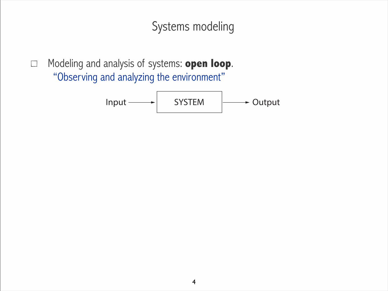
Modeling and analysis of systems: open loop. “Observing and analyzing the environment”
SYSTEMInput Output
4
Systems modeling
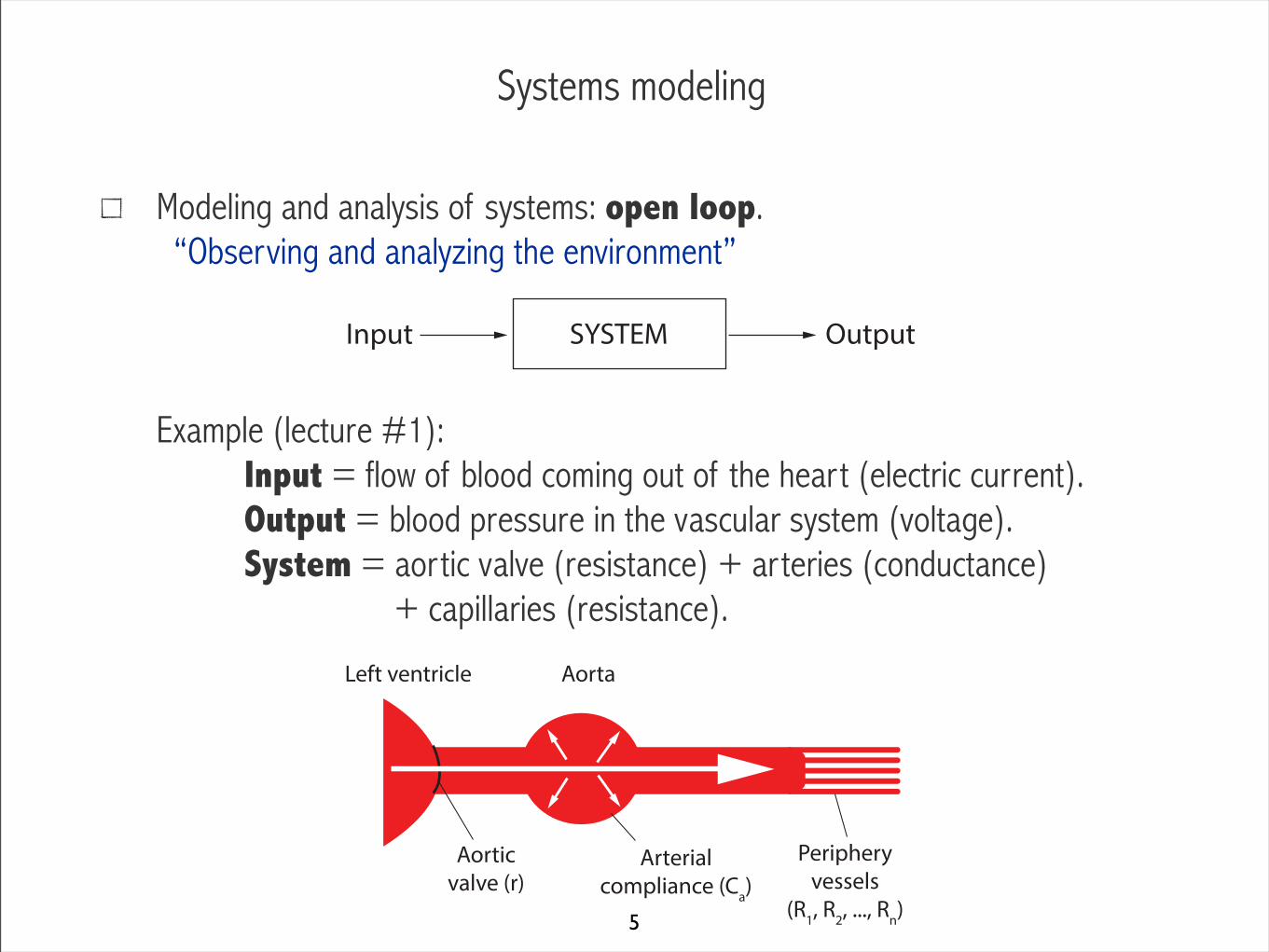
Modeling and analysis of systems: open loop. “Observing and analyzing the environment”
Example (lecture #1): Input = flow of blood coming out of the heart (electric current). Output = blood pressure in the vascular system (voltage). System = aortic valve (resistance) + arteries (conductance) + capillaries (resistance).
SYSTEMInput Output
Left ventricle
Aortic valve (r)
Aorta
Arterial compliance (Ca)
Peripheryvessels
(R1, R2, ..., Rn)
r
RCaP(t)
u(t)
PCa(t)Pr(t)
5
Systems modeling
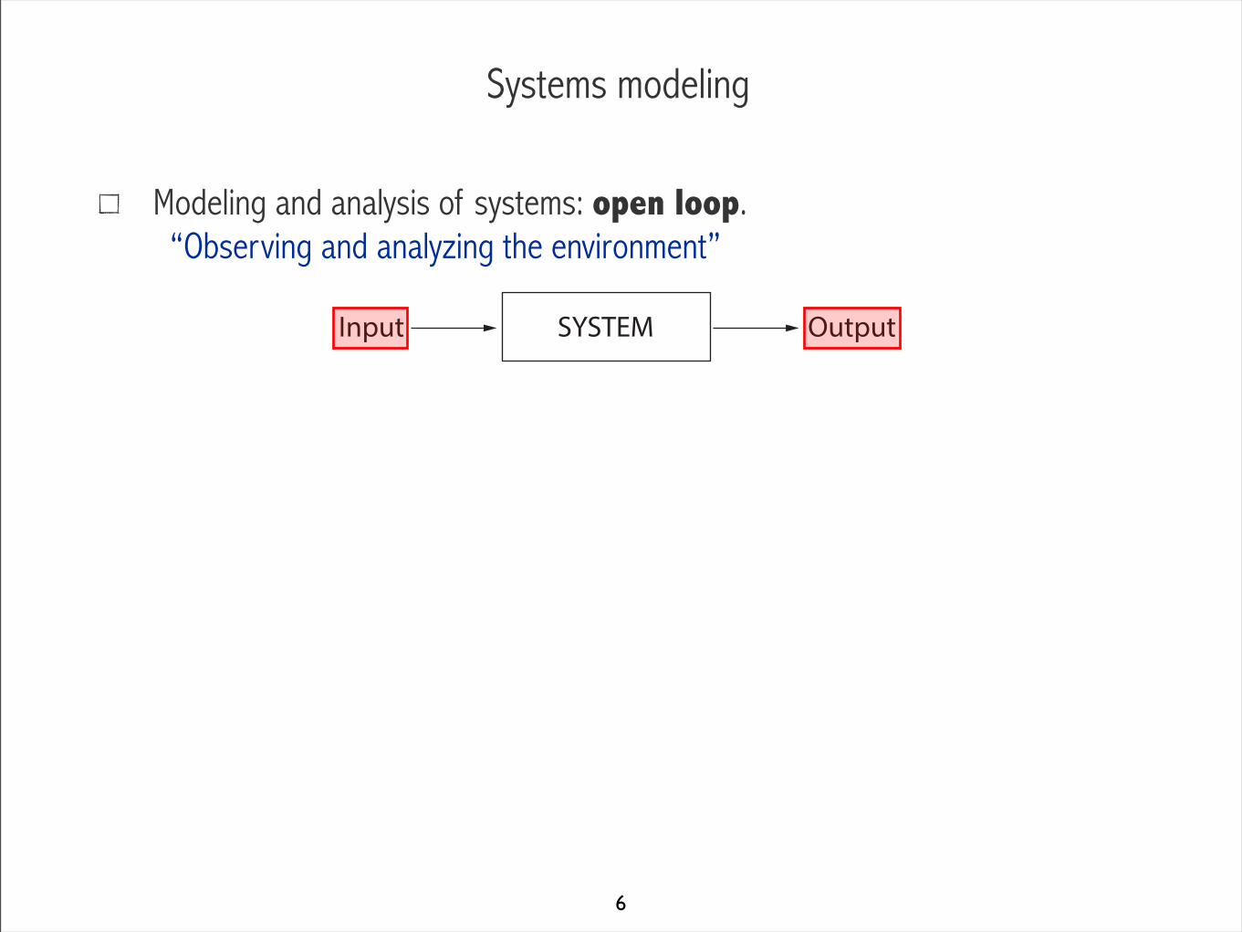
Modeling and analysis of systems: open loop. “Observing and analyzing the environment”
SYSTEMInput Output
6
Signals
Inputs and outputs are signals.Examples:
“Hi!” on a computer is “01001000 01101001 00100001” (Ascii) => Discrete, binary signal x[n].
7
Signals
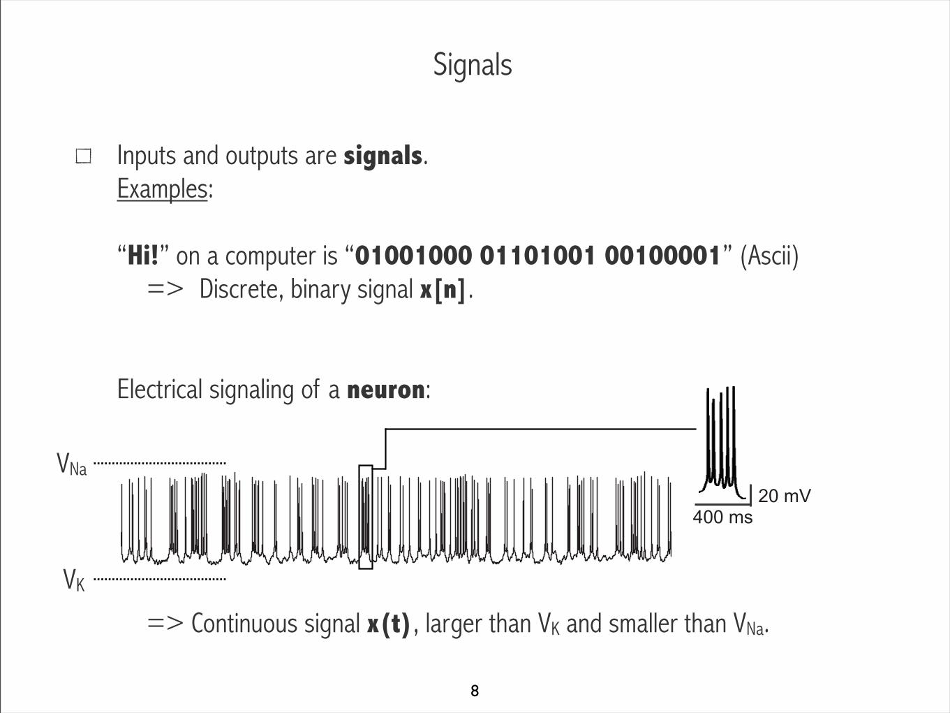
Inputs and outputs are signals.Examples:
“Hi!” on a computer is “01001000 01101001 00100001” (Ascii) => Discrete, binary signal x[n].
Electrical signaling of a neuron:
=> Continuous signal x(t), larger than VK and smaller than VNa.
400 ms20 mV
VK
VNa
8
Signals: domain and image
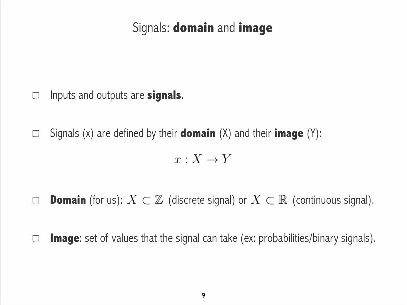
Inputs and outputs are signals.
Signals (x) are defined by their domain (X) and their image (Y):
Domain (for us): (discrete signal) or (continuous signal).
Image: set of values that the signal can take (ex: probabilities/binary signals).
9

Signals: domain and image
Inputs and outputs are signals.Examples:
“Hi!” on a computer is “01001000 01101001 00100001” (Ascii) => Discrete, binary signal x[n].
Electrical signaling of a neuron:
=> Continuous signal x(t), larger than VK and smaller than VNa.
400 ms20 mV
Domain Image
Domain Image (+⊂ℝ)
VK
VNa
10
Signals: domain and image
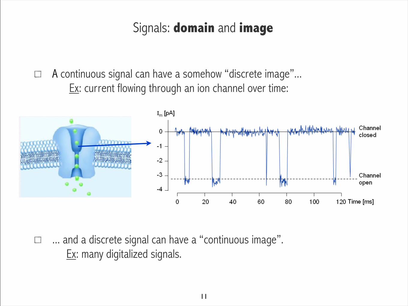
A continuous signal can have a somehow “discrete image”... Ex: current flowing through an ion channel over time:
... and a discrete signal can have a “continuous image”. Ex: many digitalized signals.
11
Why should we care about the domain of a signal?
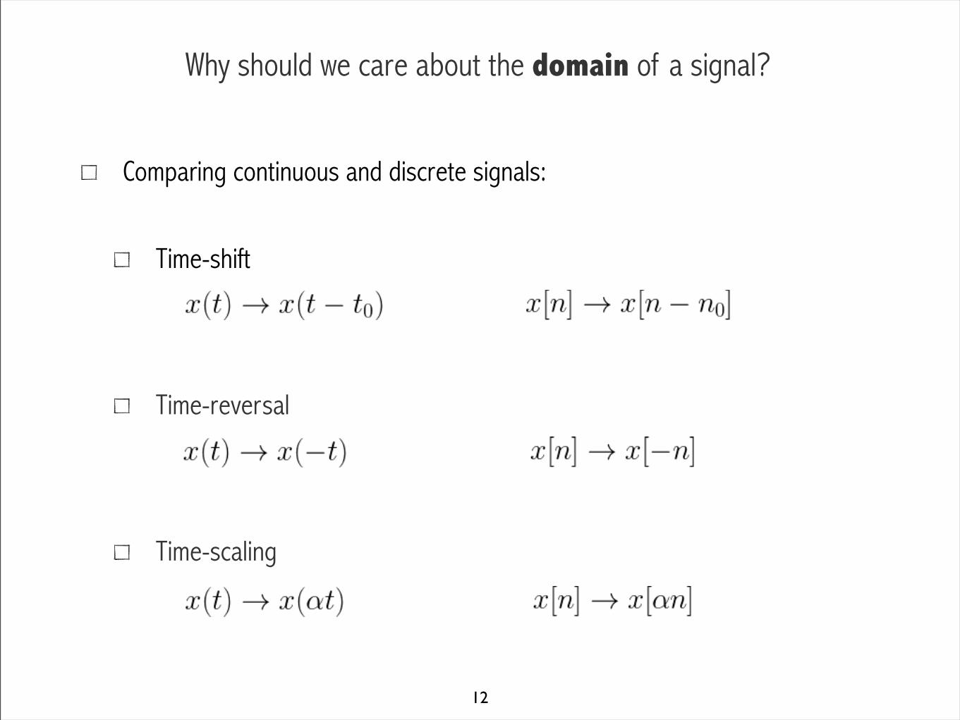
Time-shift
Time-reversal
Time-scaling
Comparing continuous and discrete signals:
12

Time-shift
Time-reversal
Time-scaling
Why should we care about the domain of a signal?
Some values of α lead to problems
Comparing continuous and discrete signals:
13

Why should we care about the image of a signal?
In theory, you can design any system using mathematical modeling.
Ex: we want to design a system that controls the movement of a robot arm for weight lifting, and proudly come up with this system that works perfectly:
But in real-life, the values that the signals can take are constrained. You have to take this limitations of the signal image into account in your model!
Ex: in the robot, the voltage signal cannot exceed some saturation voltage. With your design, the robot can barely lift his arm, let alone any additional weight...
Input voltage
Lifted weight ( relative to arm weight)
123456
14
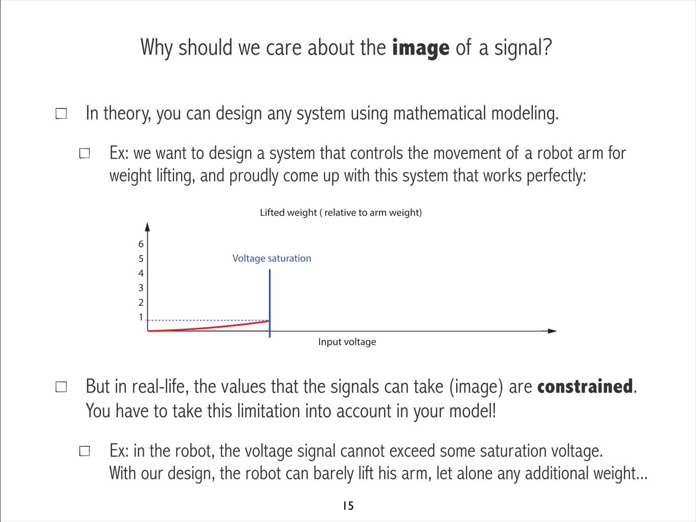
Why should we care about the image of a signal?
In theory, you can design any system using mathematical modeling.
Ex: we want to design a system that controls the movement of a robot arm for weight lifting, and proudly come up with this system that works perfectly:
But in real-life, the values that the signals can take (image) are constrained. You have to take this limitation into account in your model!
Ex: in the robot, the voltage signal cannot exceed some saturation voltage. With our design, the robot can barely lift his arm, let alone any additional weight...
Input voltage
Lifted weight ( relative to arm weight)
123456
Voltage saturation
15
Outline
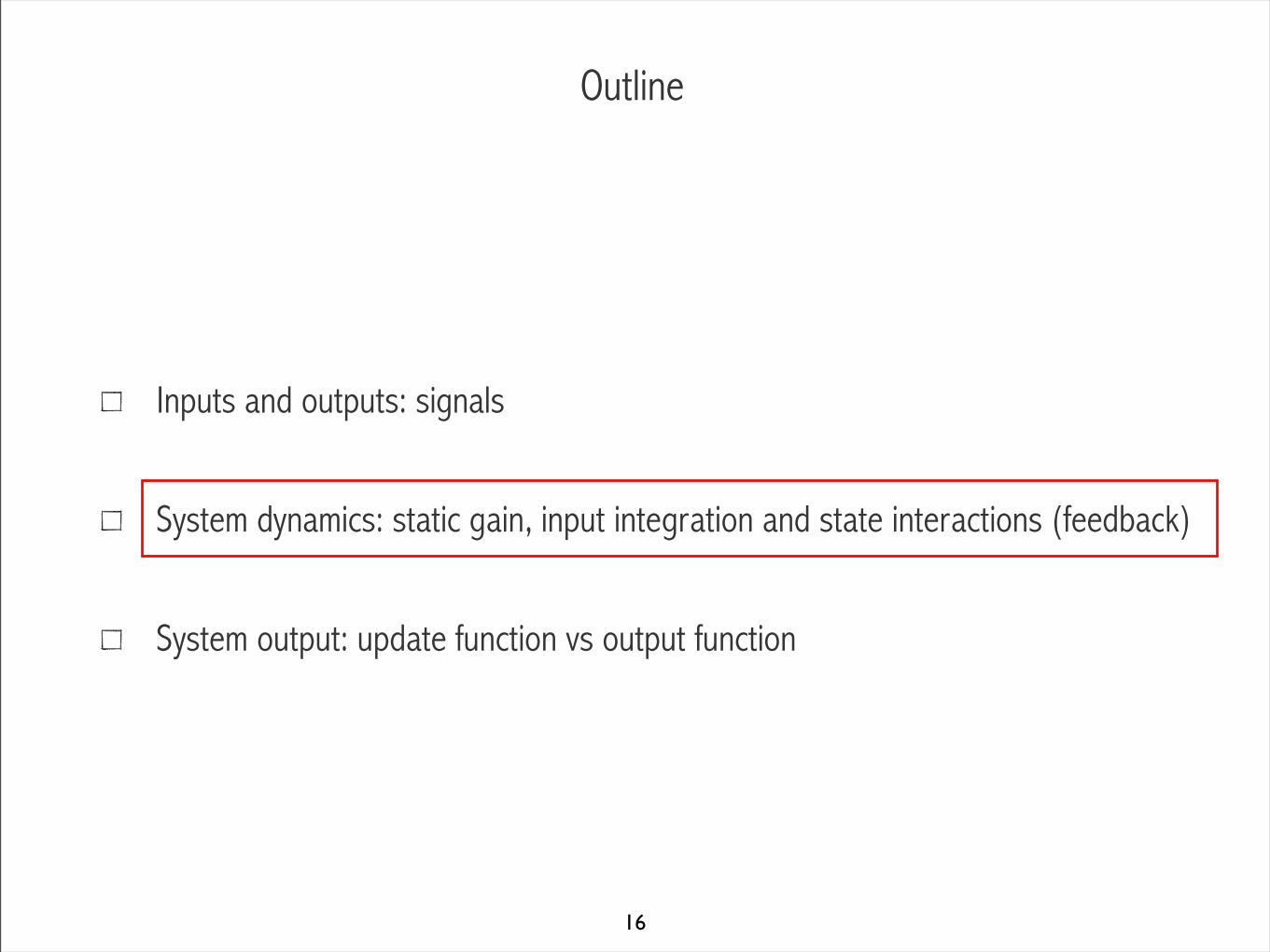
Inputs and outputs: signals
System dynamics: static gain, input integration and state interactions (feedback)
System output: update function vs output function
16
System dynamics
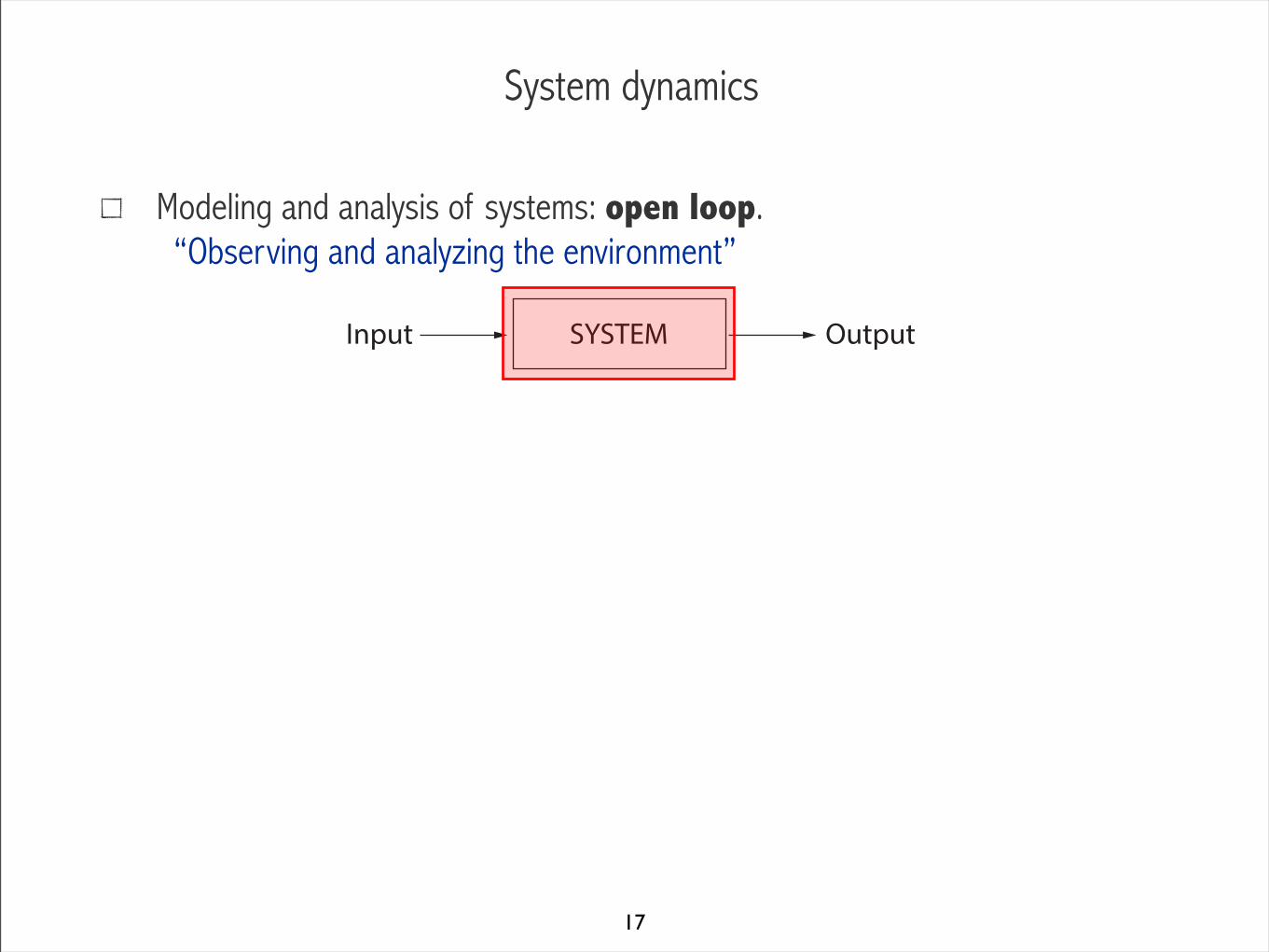
Modeling and analysis of systems: open loop. “Observing and analyzing the environment”
SYSTEMInput Output
17

System dynamics: static gain
Example #1: Applying a force on a spring.
18
kF
xF = kx () x =
1
k
F
F (Input)0
1
x (Output)
0
1/k

System dynamics: static gain
Example #1: Applying a force on a spring.
The output is solely shaped by the input at the present time: static system.
19
kF
xF = kx () x =
1
k
F
F (Input)0
1
x (Output)
0
1/kstatic gain

System dynamics: static gain
Example #2: A current through a resistive wire.
20
R
i
V = Ri () i =1
RV
static gain
i (Input)0
1
V (Output)
0
R
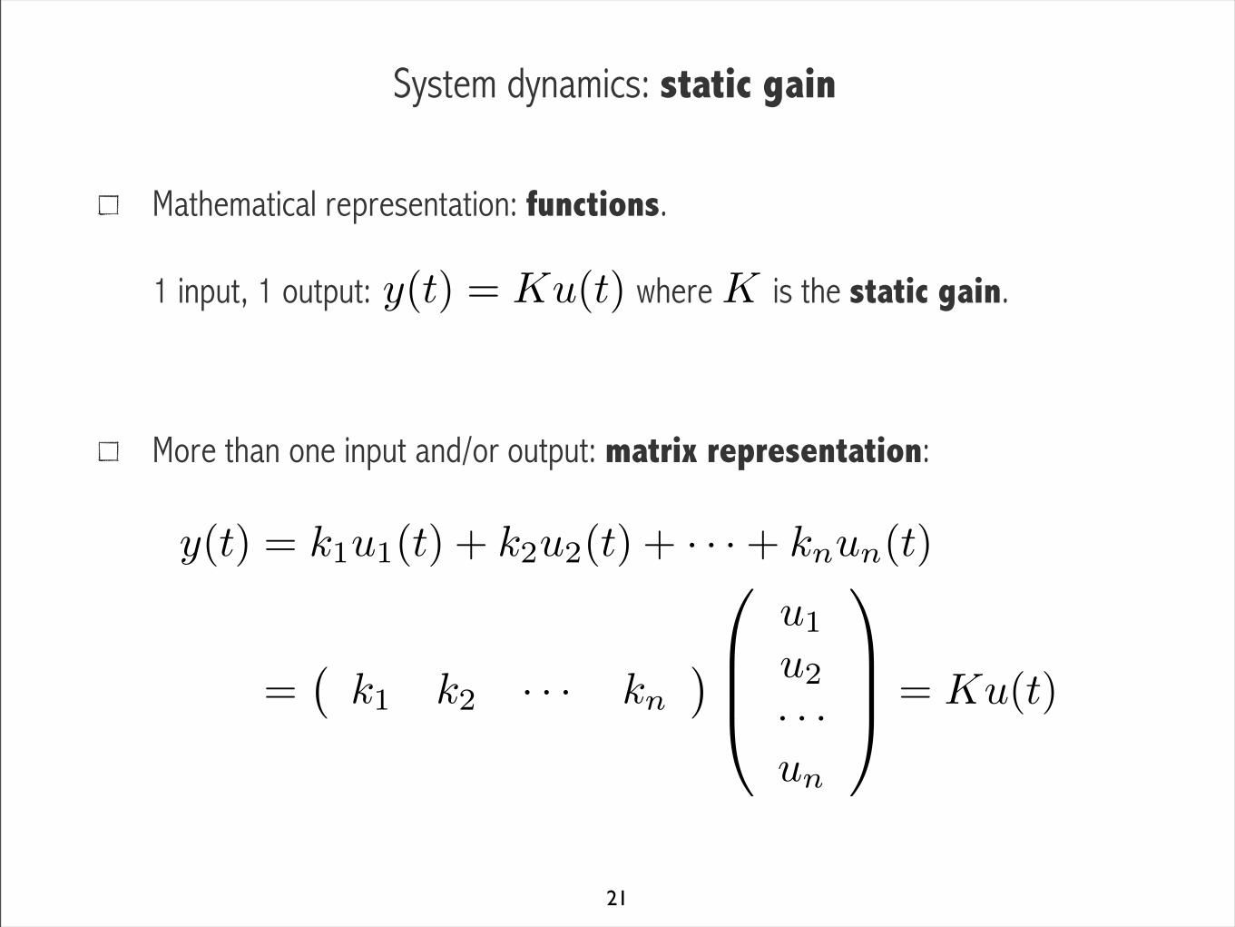
System dynamics: static gain
Mathematical representation: functions. 1 input, 1 output: where is the static gain.
More than one input and/or output: matrix representation:
21
y(t) = Ku(t) K
y(t) = k1u1(t) + k2u2(t) + · · ·+ knun(t)
=�k1 k2 · · · kn
�
0
BB@
u1
u2
· · ·un
1
CCA = Ku(t)
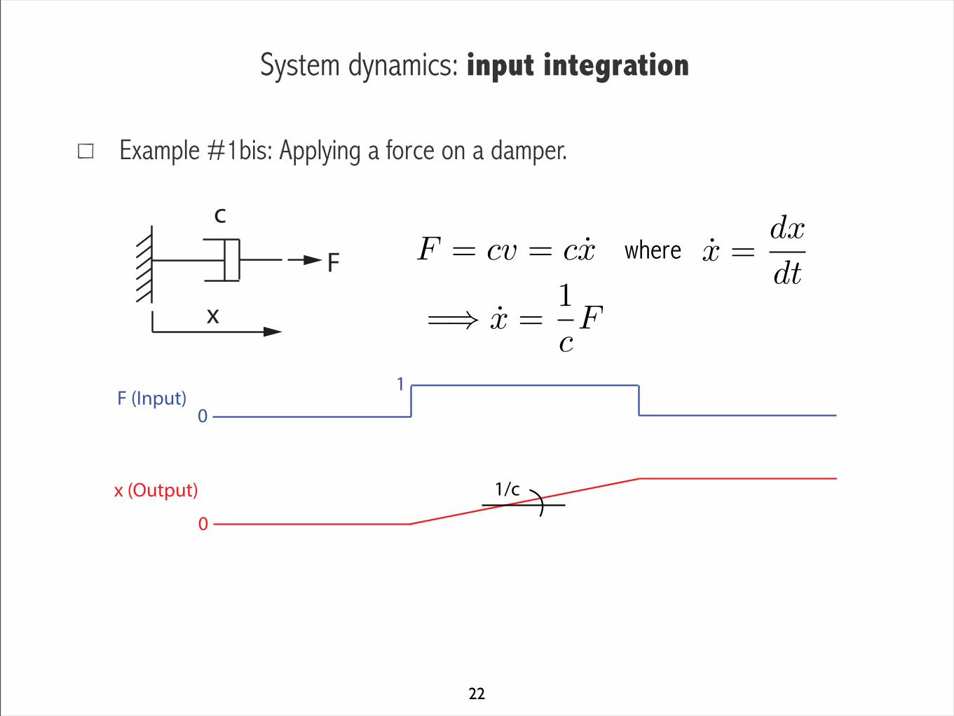
System dynamics: input integration
Example #1bis: Applying a force on a damper.
22
F
x
cF = cv = cx
wherex =
dx
dt
=) x =1
c
F
F (Input)0
1
x (Output)
0
1/c
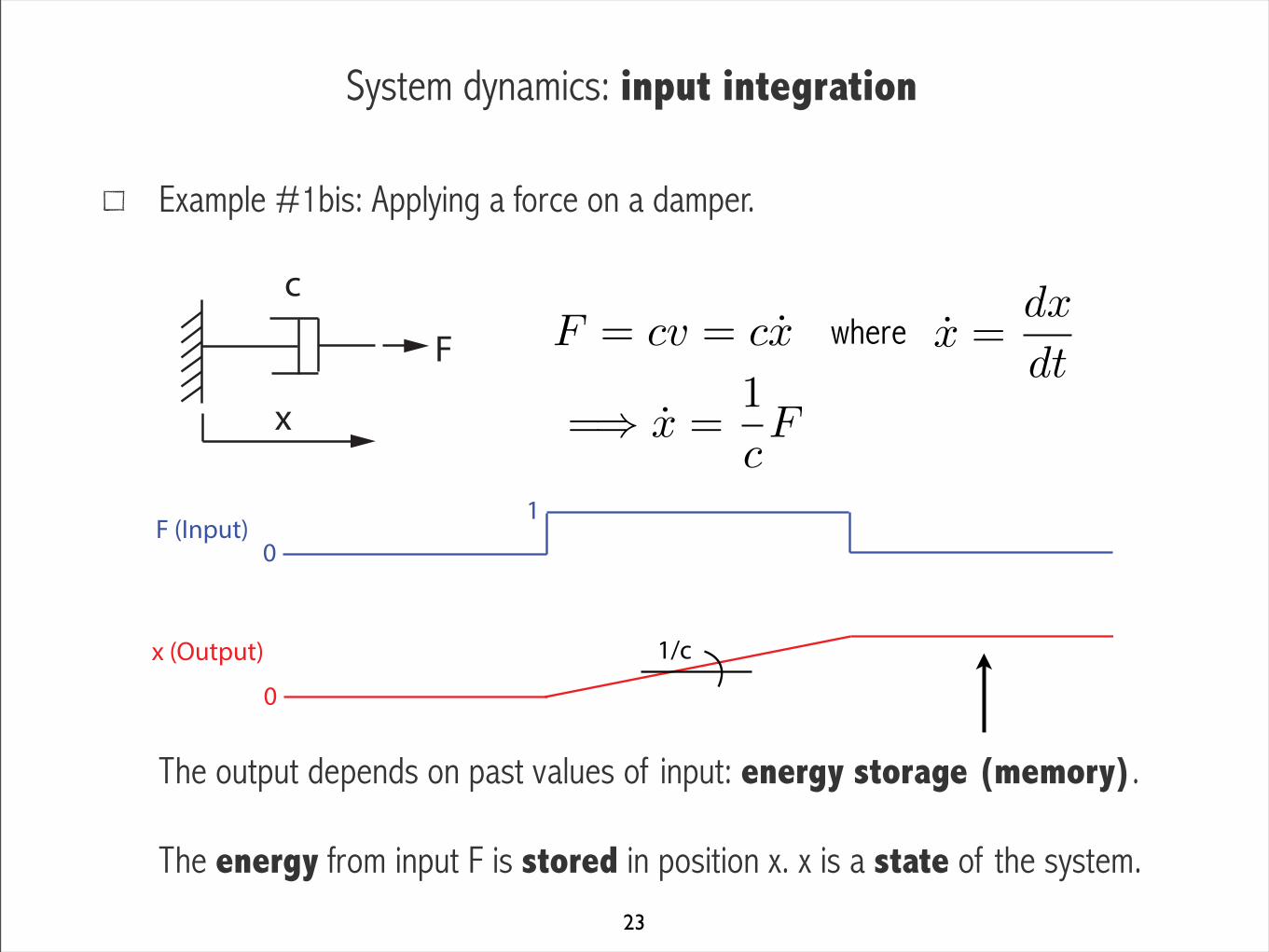
System dynamics: input integration
Example #1bis: Applying a force on a damper.
The output depends on past values of input: energy storage (memory).
The energy from input F is stored in position x. x is a state of the system.
23
F
x
cF = cv = cx
wherex =
dx
dt
=) x =1
c
F
F (Input)0
1
x (Output)
0
1/c

System dynamics: input integration
Example #2bis: A current “through” a capacitor.
The energy from input i is stored in voltage V. V is a state of the system.
24
i
C i = CV () V =1
Ci
i (Input)0
1
V (Output)
0
1/C

System dynamics: input integration
Integrators store past values of the input into states.
Mathematical representation: ordinary differential equations (continuous). or difference equations (discrete).
25
Input
State
x = Bu
x[n+ 1] = Bu[n]or
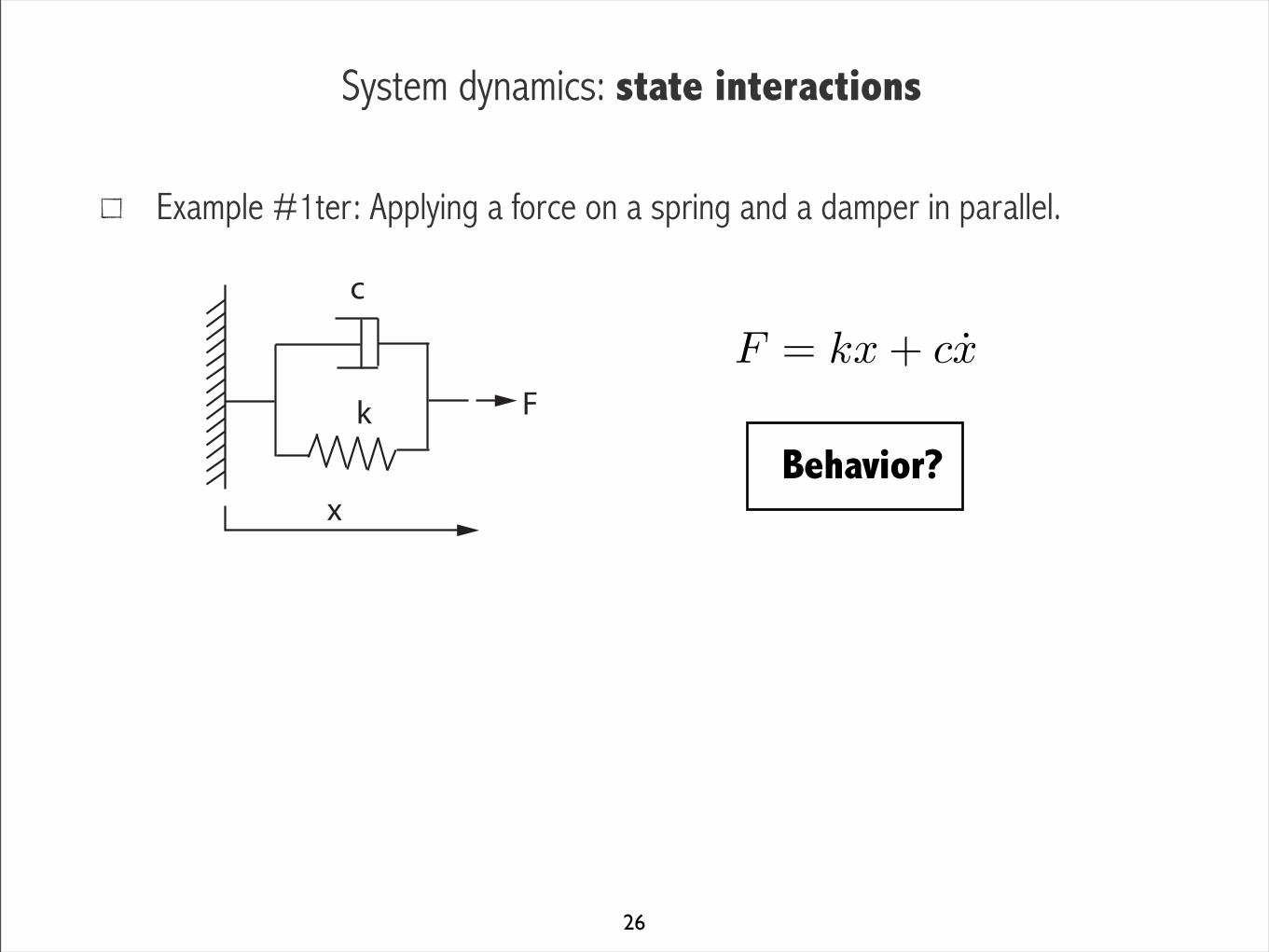
System dynamics: state interactions
Example #1ter: Applying a force on a spring and a damper in parallel.
26
k
c
x
F
F = kx+ cx
Behavior?
System dynamics: state interactions
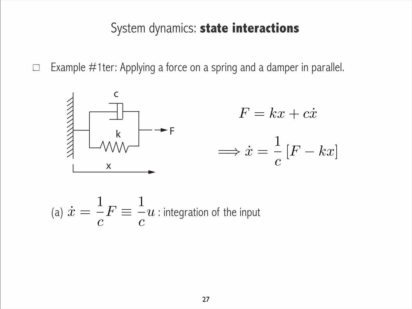
Example #1ter: Applying a force on a spring and a damper in parallel.
(a) : integration of the input
27
k
c
x
F
F = kx+ cx
=) x =1
c
[F � kx]
x =1
c
F ⌘ 1
c
u

System dynamics: state interactions
Example #1ter: Applying a force on a spring and a damper in parallel.
(a) : integration of the input
(b) : does not depend on input - Internal dynamics!
28
k
c
x
F
F = kx+ cx
=) x =1
c
[F � kx]
x =1
c
F ⌘ 1
c
u
x = �k
c
x
System dynamics: state interactions
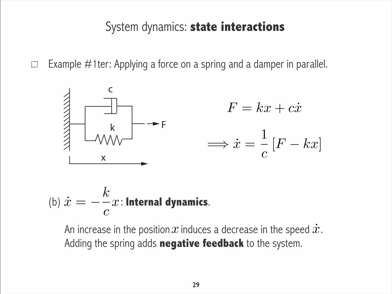
Example #1ter: Applying a force on a spring and a damper in parallel.
(b) : Internal dynamics.
An increase in the position induces a decrease in the speed . Adding the spring adds negative feedback to the system.
29
k
c
x
F
F = kx+ cx
=) x =1
c
[F � kx]
x = �k
c
x
x
x

System dynamics: state interactions
Example #1ter: Applying a force on a spring and a damper in parallel.
30
k
c
x
F
F = kx+ cx
=) x =1
c
[F � kx]
F (Input)0
1
x (Output)
0
?

System dynamics: state interactions
Example #2ter: Applying an input voltage on an RC circuit.
(a) : integration of the input
(b) : Internal dynamics.
31
R
i
VC
i
i = iR + iC =V
R+ CV
=) V =1
C
i� V
R
�
V =1
Ci
V = � 1
RCV
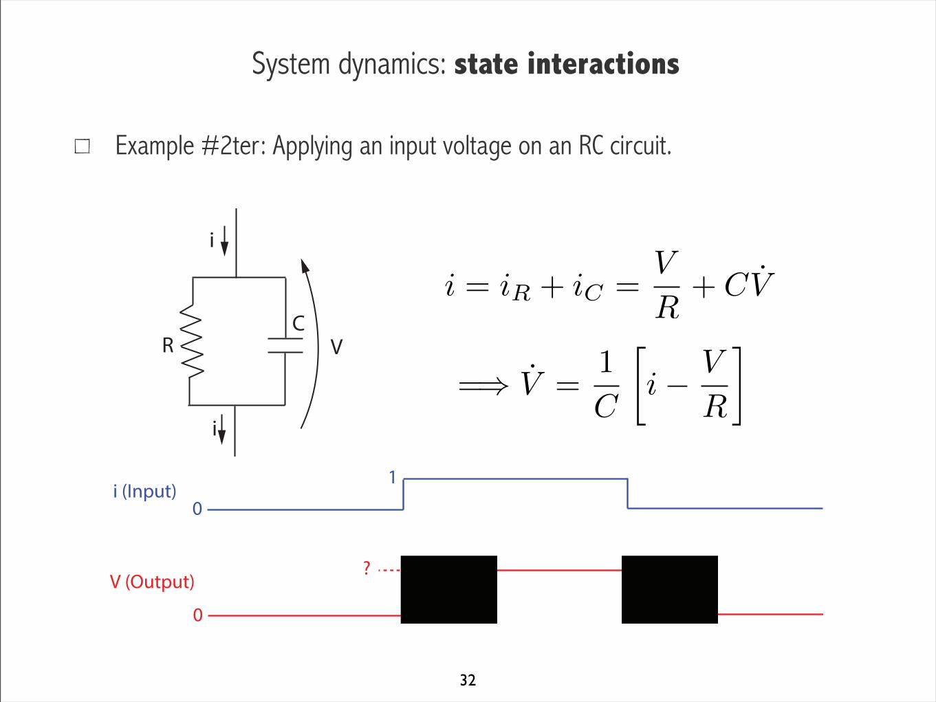
System dynamics: state interactions
Example #2ter: Applying an input voltage on an RC circuit.
32
R
i
VC
i
i = iR + iC =V
R+ CV
=) V =1
C
i� V
R
�
i (Input)0
1
V (Output)
0
?

System dynamics: state interactions
Mechanical system vs electrical system.
33
=) V =1
C
i� V
R
�=) x =
1
c
[F � kx]
Mechanical system Electrical system
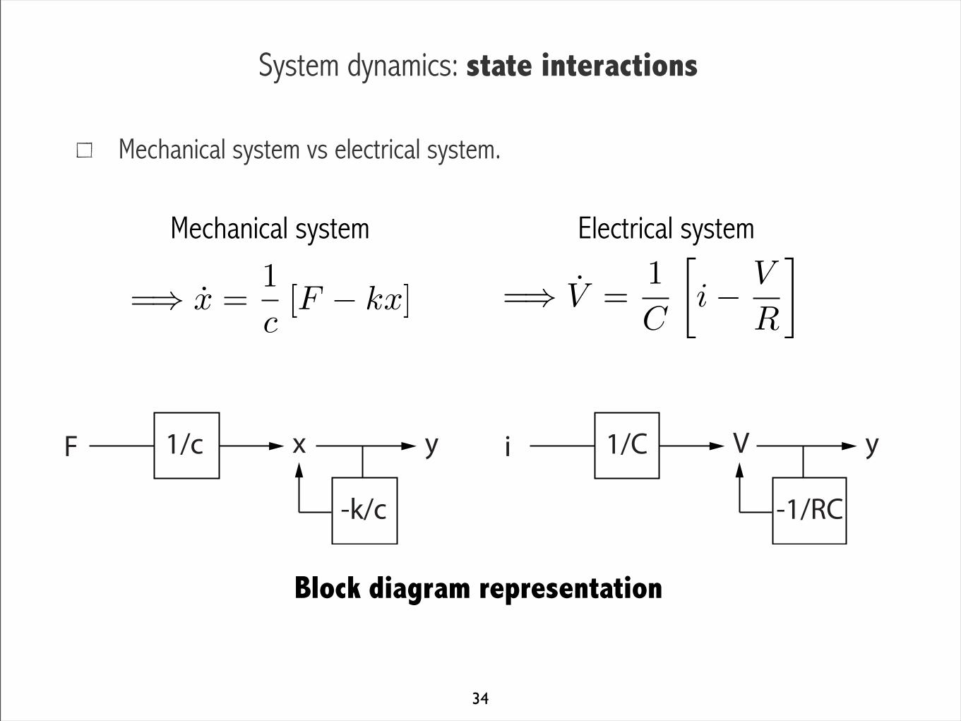
System dynamics: state interactions
Mechanical system vs electrical system.
34
=) V =1
C
i� V
R
�=) x =
1
c
[F � kx]
Mechanical system Electrical system
F 1/c x
-k/c
y i 1/C V
-1/RC
y
Block diagram representation
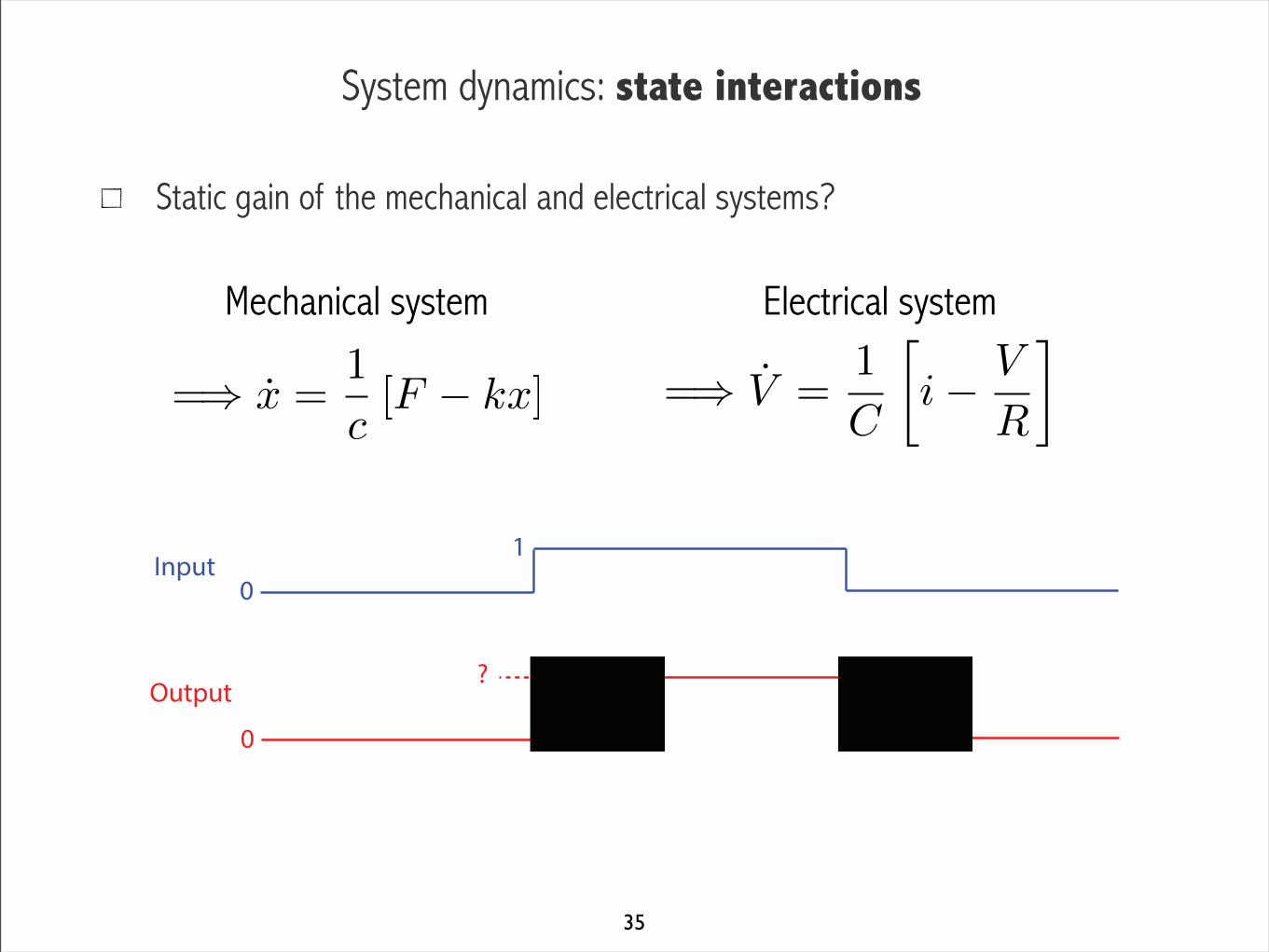
System dynamics: state interactions
Static gain of the mechanical and electrical systems?
35
=) V =1
C
i� V
R
�=) x =
1
c
[F � kx]
Mechanical system Electrical system
Input0
1
Output
0
?
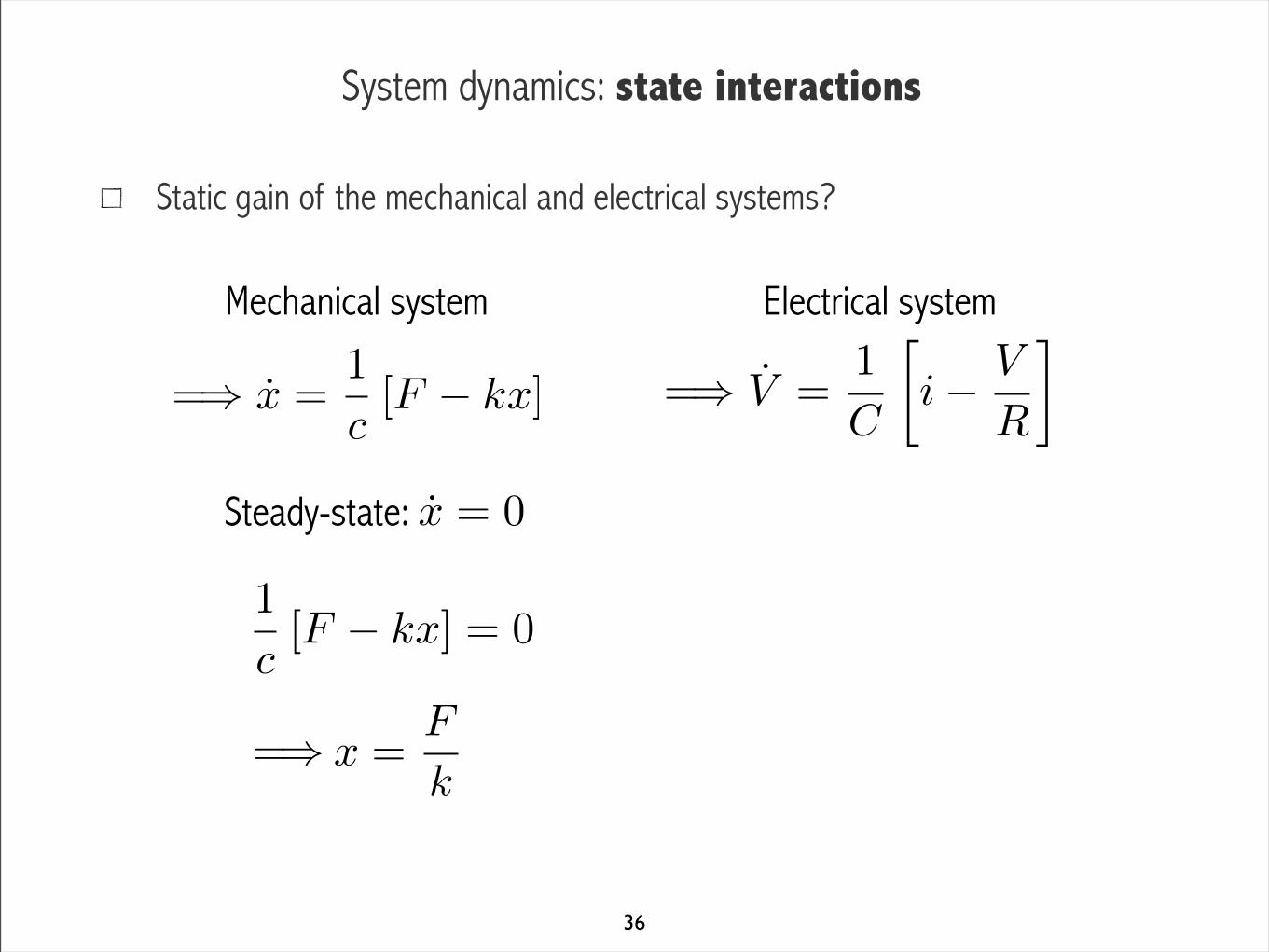
System dynamics: state interactions
Static gain of the mechanical and electrical systems?
36
=) V =1
C
i� V
R
�=) x =
1
c
[F � kx]
Mechanical system Electrical system
Steady-state: x = 0
x =F
k
1
c
[F � kx] = 0
=)
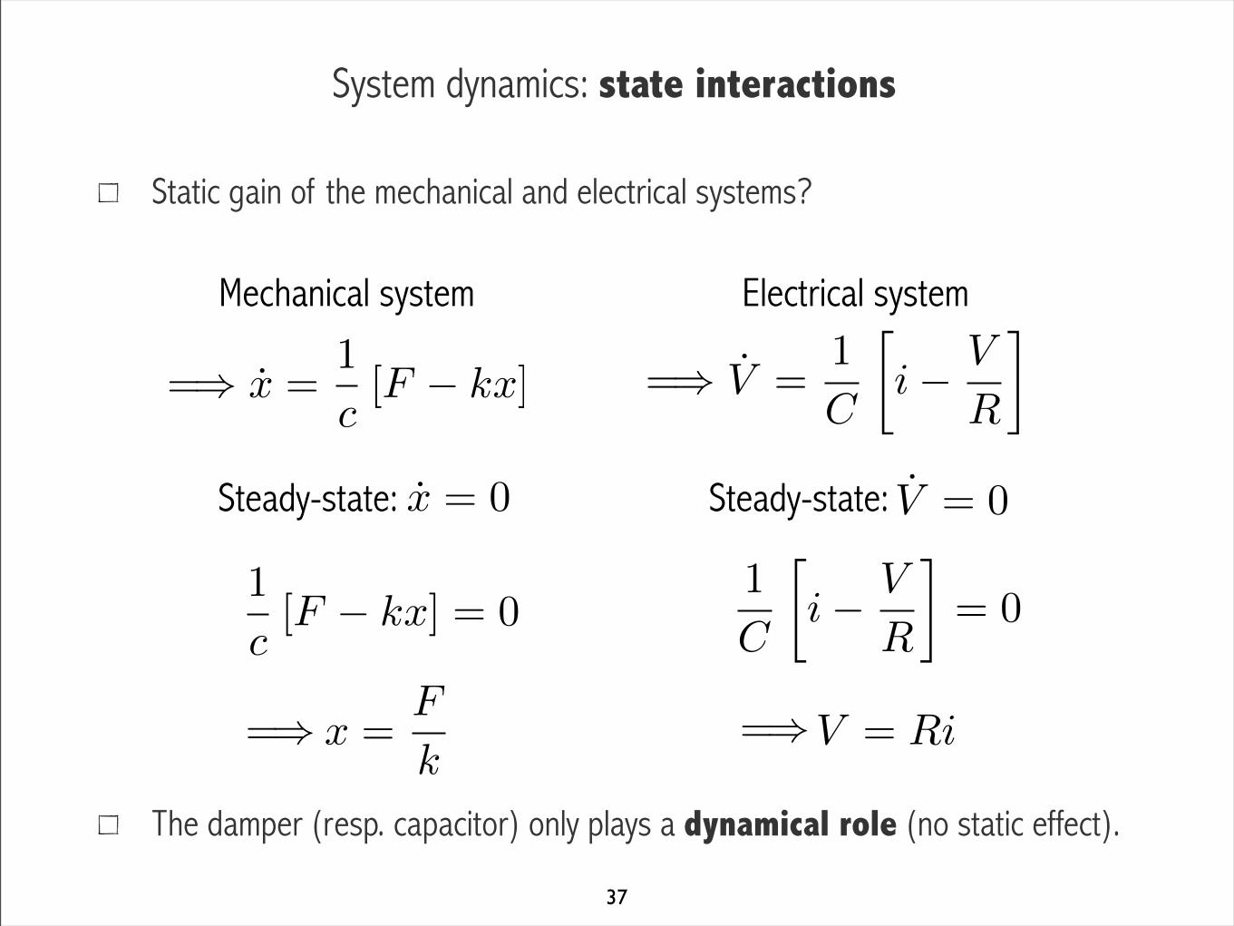
System dynamics: state interactions
Static gain of the mechanical and electrical systems?
The damper (resp. capacitor) only plays a dynamical role (no static effect).
37
=) V =1
C
i� V
R
�=) x =
1
c
[F � kx]
Mechanical system Electrical system
Steady-state: Steady-state: x = 0 V = 0
V = Ri
1
C
i� V
R
�= 0
x =F
k
1
c
[F � kx] = 0
=) =)
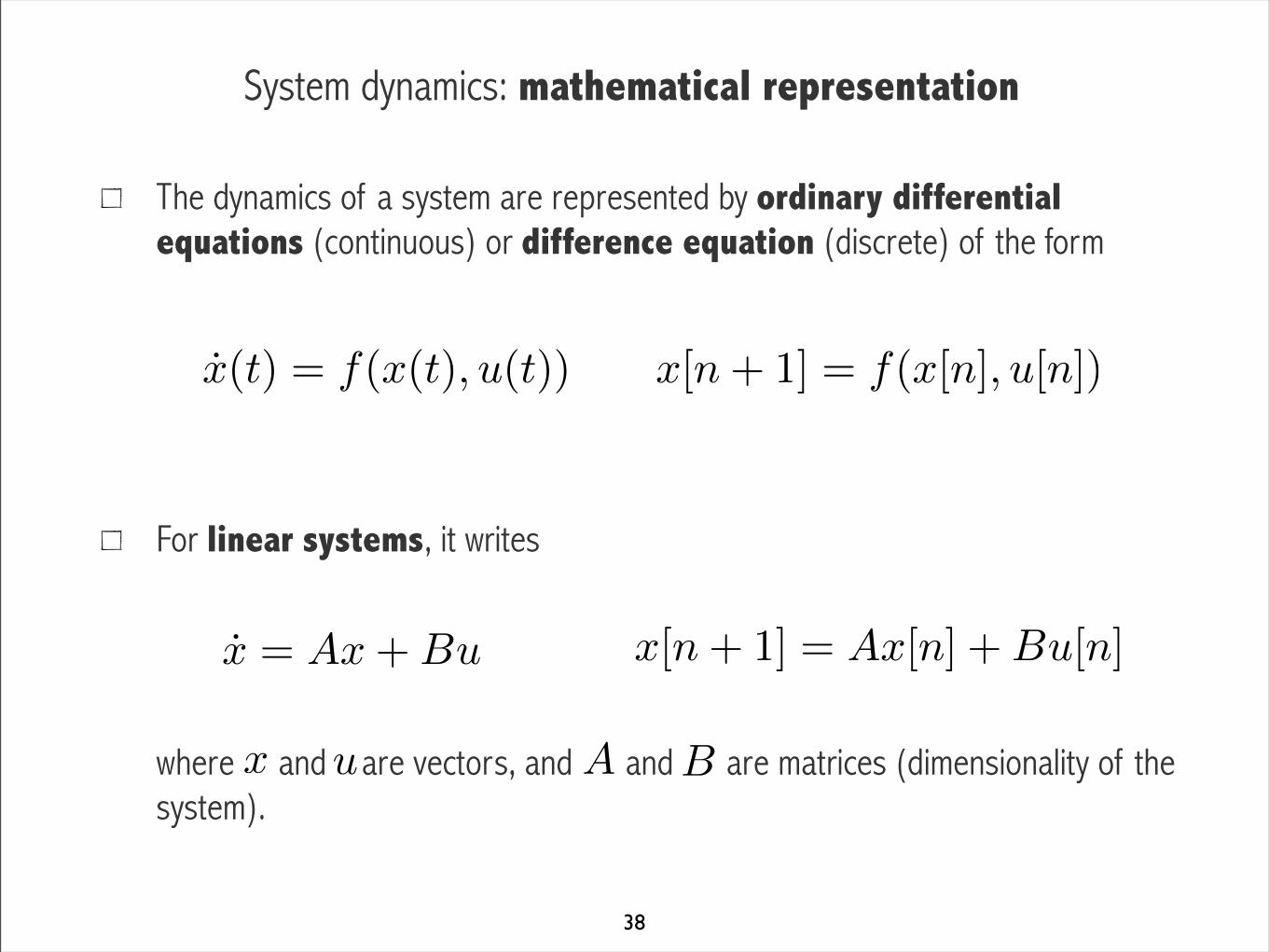
System dynamics: mathematical representation
The dynamics of a system are represented by ordinary differential equations (continuous) or difference equation (discrete) of the form
For linear systems, it writes
where and are vectors, and and are matrices (dimensionality of the system).
38
x(t) = f(x(t), u(t)) x[n+ 1] = f(x[n], u[n])
x = Ax+Bu
x[n+ 1] = Ax[n] +Bu[n]
BAx u
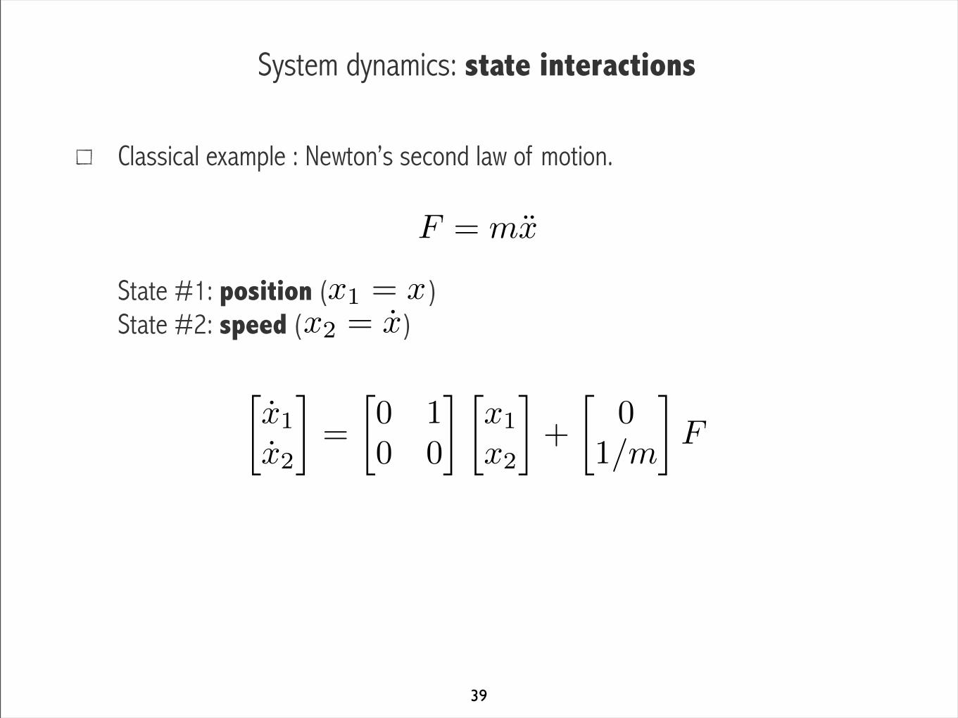
System dynamics: state interactions
Classical example : Newton’s second law of motion.
State #1: position ( )State #2: speed ( )
39
F = mx
x2 = x
x1 = x
x1
x2
�=
0 10 0
� x1
x2
�+
0
1/m
�F

System dynamics: state interactions
Classical example : Newton’s second law of motion.
State #1: position ( )State #2: speed ( )
40
F = mx
x2 = x
x1 = x
x1
x2
�=
0 10 0
� x1
x2
�+
0
1/m
�F
Force affects speed(Input integration)
Speed affects position(state interactions)
Outline
Inputs and outputs: signals
System dynamics: static gain, input integration and state interactions (feedback)
System output: update function vs output function
41
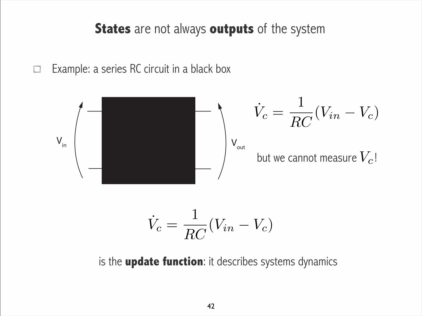
States are not always outputs of the system
Example: a series RC circuit in a black box
but we cannot measure !
is the update function: it describes systems dynamics
42
R Vout
C
i
Vin
Vc =1
RC(Vin � Vc)
Vc
Vc =1
RC(Vin � Vc)
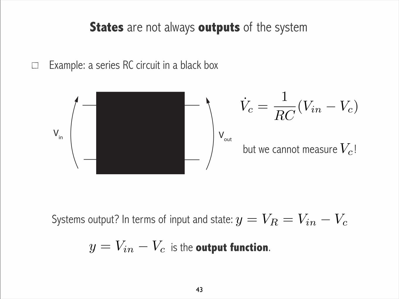
States are not always outputs of the system
Example: a series RC circuit in a black box
but we cannot measure !
Systems output? In terms of input and state:
is the output function.
43
R Vout
C
i
Vin
Vc =1
RC(Vin � Vc)
Vc
y = VR = Vin � Vc
y = Vin � Vc
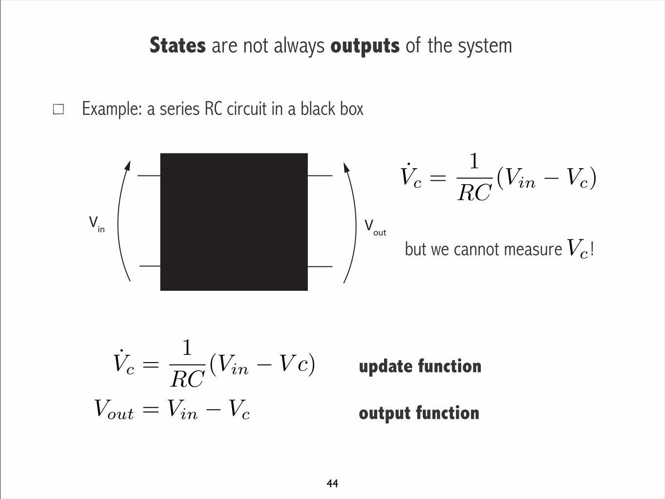
States are not always outputs of the system
Example: a series RC circuit in a black box
but we cannot measure !
update function output function
44
R Vout
C
i
Vin
Vc =1
RC(Vin � Vc)
Vc
Vc
=1
RC(V
in
� V c)
Vout
= Vin
� Vc
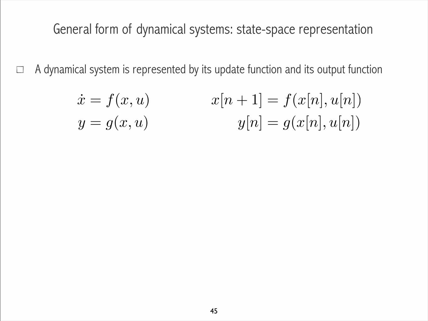
General form of dynamical systems: state-space representation
45
A dynamical system is represented by its update function and its output function
For linear systems, it writes
where , and are vectors,
, , and are matrices (dimensionality of the system).
x = f(x, u)
y = g(x, u)
x = Ax+Bu
y = Cx+Du
BA
x u y
DC
x[n+ 1] = Ax[n] +Bu[n]
y[n] = Cx[n] +Du[n]
x[n+ 1] = f(x[n], u[n])
y[n] = g(x[n], u[n])
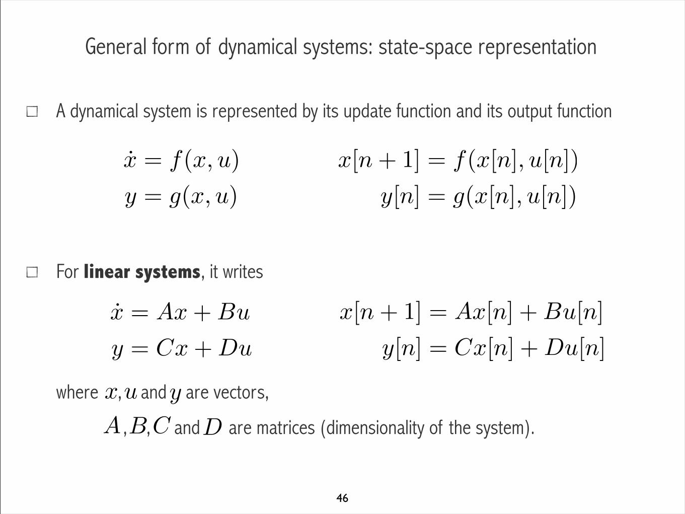
General form of dynamical systems: state-space representation
46
A dynamical system is represented by its update function and its output function
For linear systems, it writes
where , and are vectors,
, , and are matrices (dimensionality of the system).
x = f(x, u)
y = g(x, u)
x = Ax+Bu
y = Cx+Du
BA
x u y
DC
x[n+ 1] = Ax[n] +Bu[n]
y[n] = Cx[n] +Du[n]
x[n+ 1] = f(x[n], u[n])
y[n] = g(x[n], u[n])

Linear systems: A,B,C,D representation
Linear, time-invariant (LTI) dynamical systems can be represented in the form
where describes how the dynamics of the system evolve (dynamics matrix) describes how the input influences the states (input matrix) describes how the states “are seen” in the output (output matrix). describes how the input directly influences the output (feedthrough matrix).
The output is therefore a function of the input and the states. Simple but recurrent case: the output is one of the states.
47
x = Ax+Bu
y = Cx+Du
BA
DC

Linear systems: block diagram representation
48
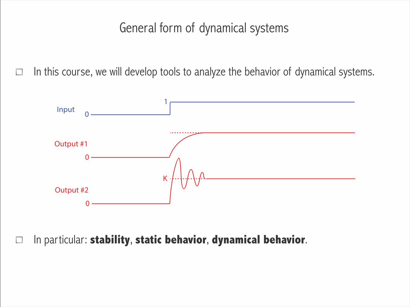
General form of dynamical systems
In this course, we will develop tools to analyze the behavior of dynamical systems.
In particular: stability, static behavior, dynamical behavior.
Input 0
1
Output #1
0
Output #2
0
K
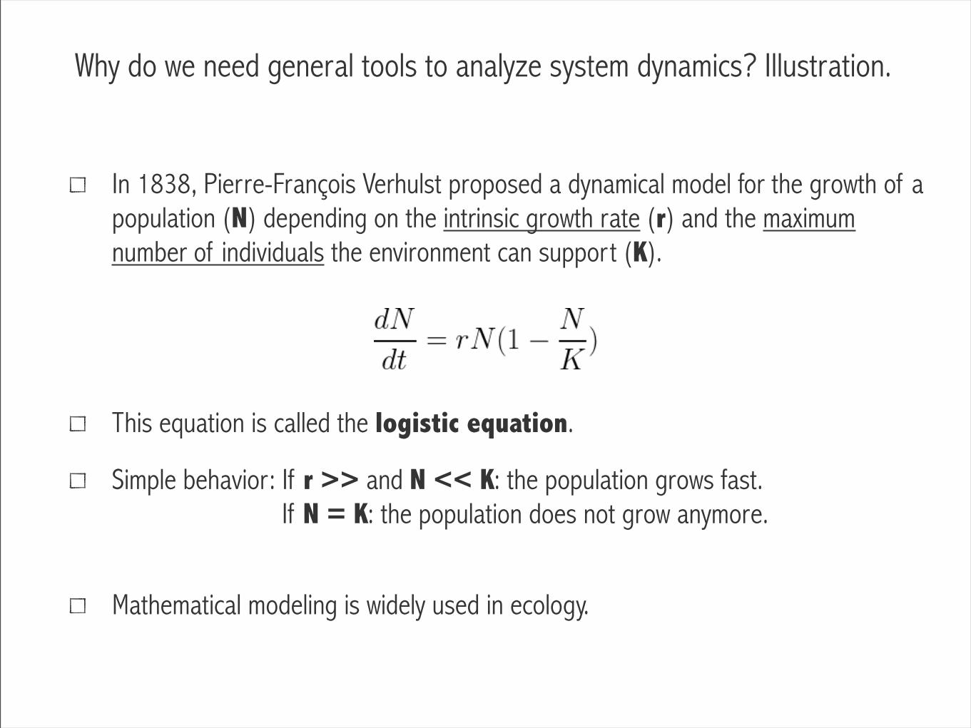
Why do we need general tools to analyze system dynamics? Illustration.
In 1838, Pierre-François Verhulst proposed a dynamical model for the growth of a population (N) depending on the intrinsic growth rate (r) and the maximum number of individuals the environment can support (K).
This equation is called the logistic equation.
Simple behavior: If r >> and N << K: the population grows fast. If N = K: the population does not grow anymore.
Mathematical modeling is widely used in ecology.

The logistic equation
Simulation of the logistic equation for different growth rates and K=1.
1 1.5 2 2.5 3 3.5 4 4.5 50
0.2
0.4
0.6
0.8
1Logistic equation, r=2
1 1.5 2 2.5 3 3.5 4 4.5 50
0.2
0.4
0.6
0.8
1Logistic equation,r=4
time
N
N
51

A discrete equivalent of the logistic equation: the logistic map
In 1976, Robert May proposed a “discrete equivalent”
As opposed to the continuous system, the dynamics of the discrete system is extremely rich, and can be “chaotic” for certain values of α.
vs
52
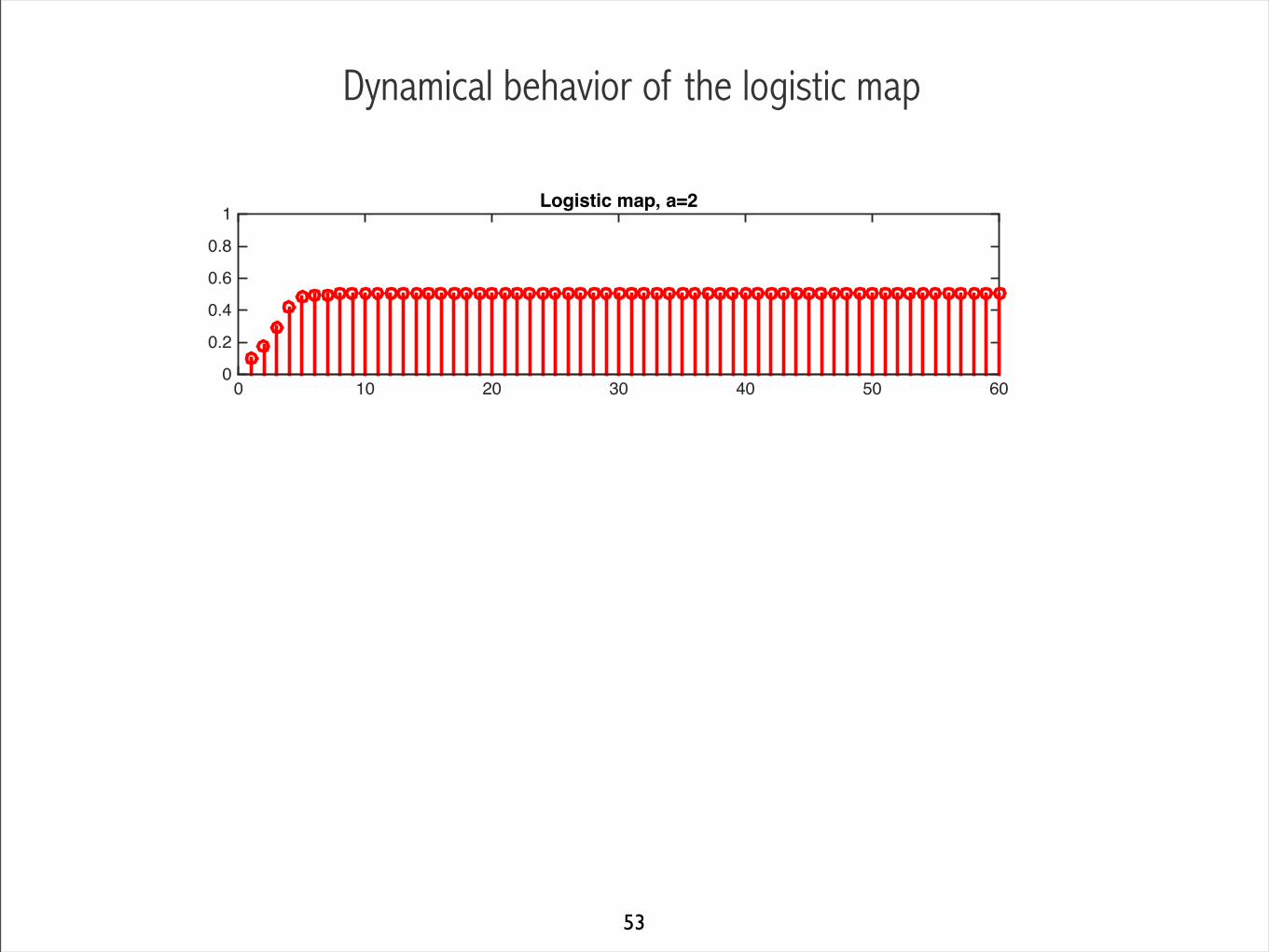
Dynamical behavior of the logistic map
0 10 20 30 40 50 600
0.2
0.4
0.6
0.8
1Logistic map, a=2
0 10 20 30 40 50 600
0.2
0.4
0.6
0.8
1Logistic map, a=3.3
0 10 20 30 40 50 600
0.2
0.4
0.6
0.8
1Logistic map, a=4
53
Dynamical behavior of the logistic map
0 10 20 30 40 50 600
0.2
0.4
0.6
0.8
1Logistic map, a=2
0 10 20 30 40 50 600
0.2
0.4
0.6
0.8
1Logistic map, a=3.3
0 10 20 30 40 50 600
0.2
0.4
0.6
0.8
1Logistic map, a=4
54
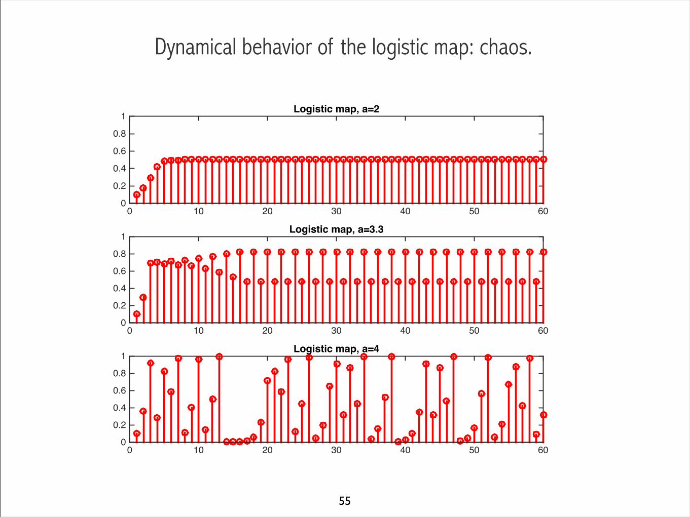
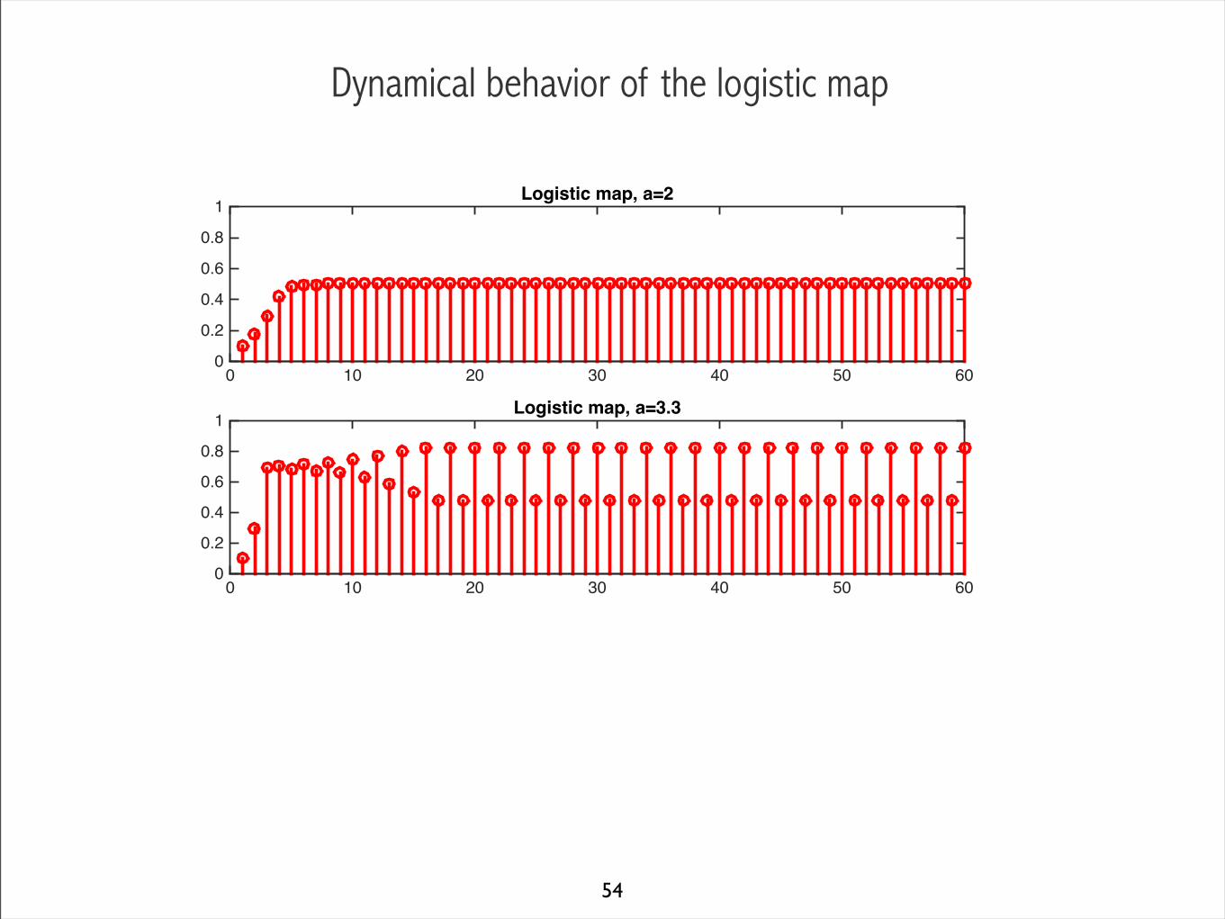
Dynamical behavior of the logistic map: chaos.
0 10 20 30 40 50 600
0.2
0.4
0.6
0.8
1Logistic map, a=2
0 10 20 30 40 50 600
0.2
0.4
0.6
0.8
1Logistic map, a=3.3
0 10 20 30 40 50 600
0.2
0.4
0.6
0.8
1Logistic map, a=4
55
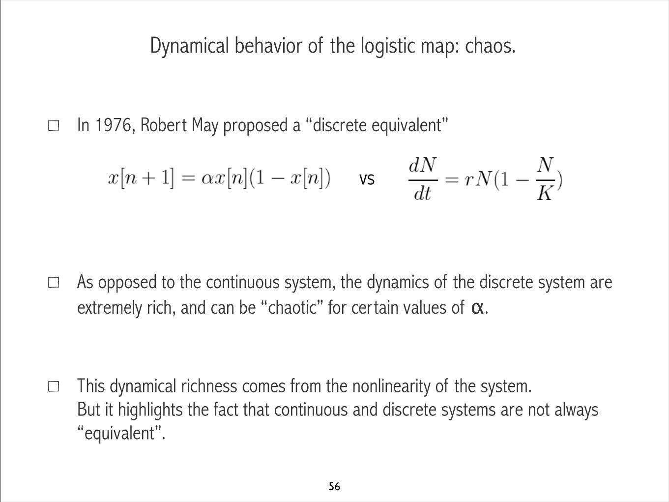
Dynamical behavior of the logistic map: chaos.
In 1976, Robert May proposed a “discrete equivalent”
As opposed to the continuous system, the dynamics of the discrete system are extremely rich, and can be “chaotic” for certain values of α.
This dynamical richness comes from the nonlinearity of the system.But it highlights the fact that continuous and discrete systems are not always “equivalent”.
vs
56

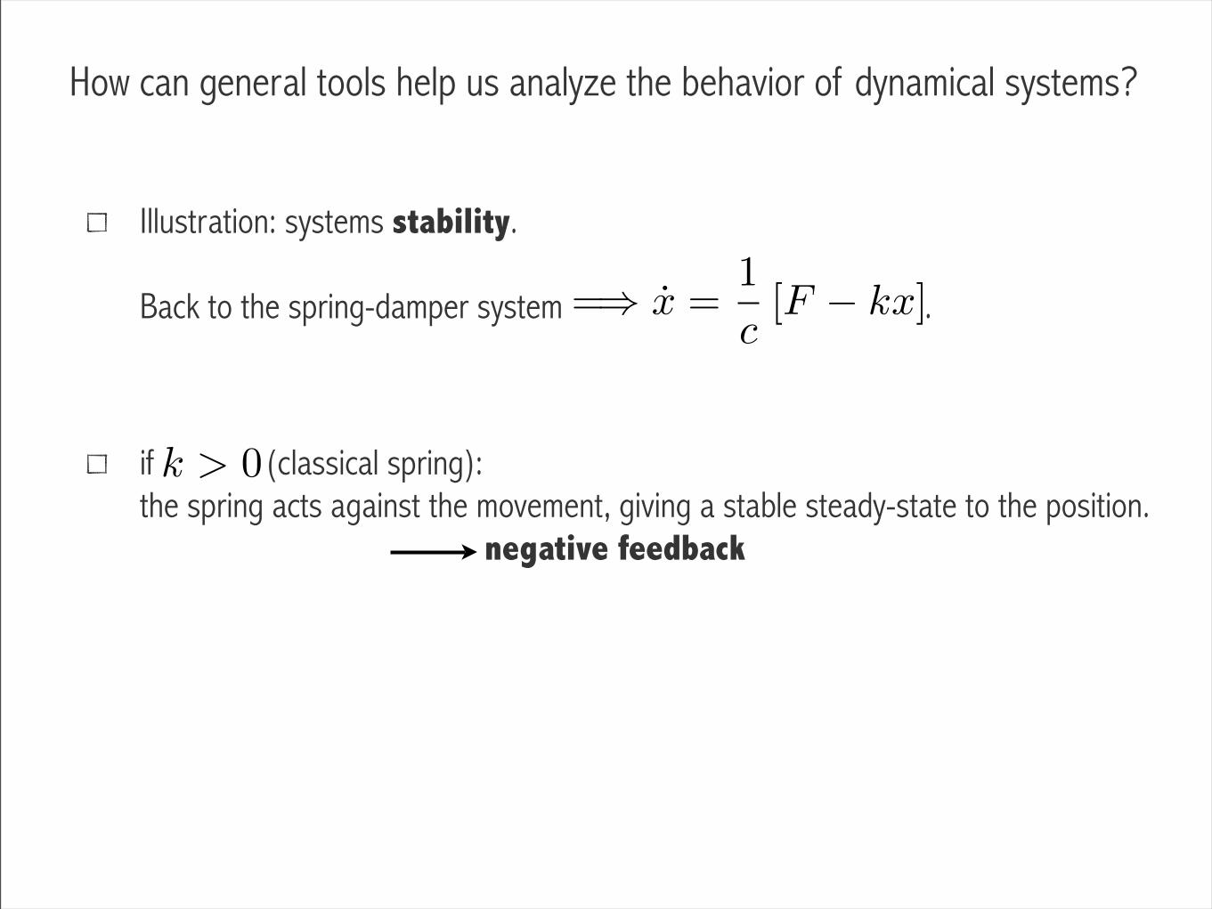
How can general tools help us analyze the behavior of dynamical systems?
Illustration: systems stability.
Back to the spring-damper system .
if (classical spring):the spring acts against the movement, giving a stable steady-state to the position. negative feedback
if :the further the system is, the faster is goes away.the system will go away until the “negative spring” saturates. positive feedback
=) x =1
c
[F � kx]
k > 0
k < 0
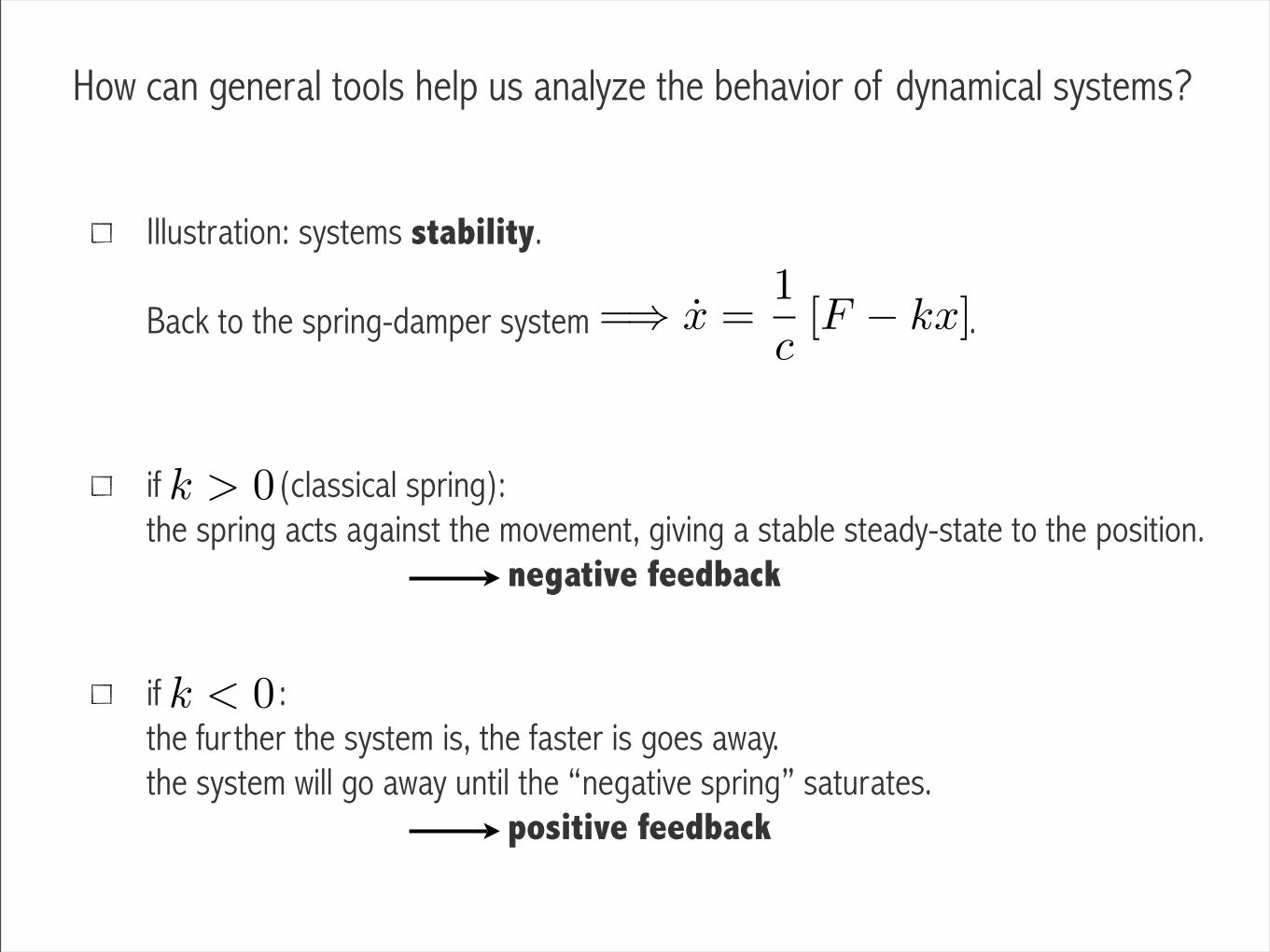
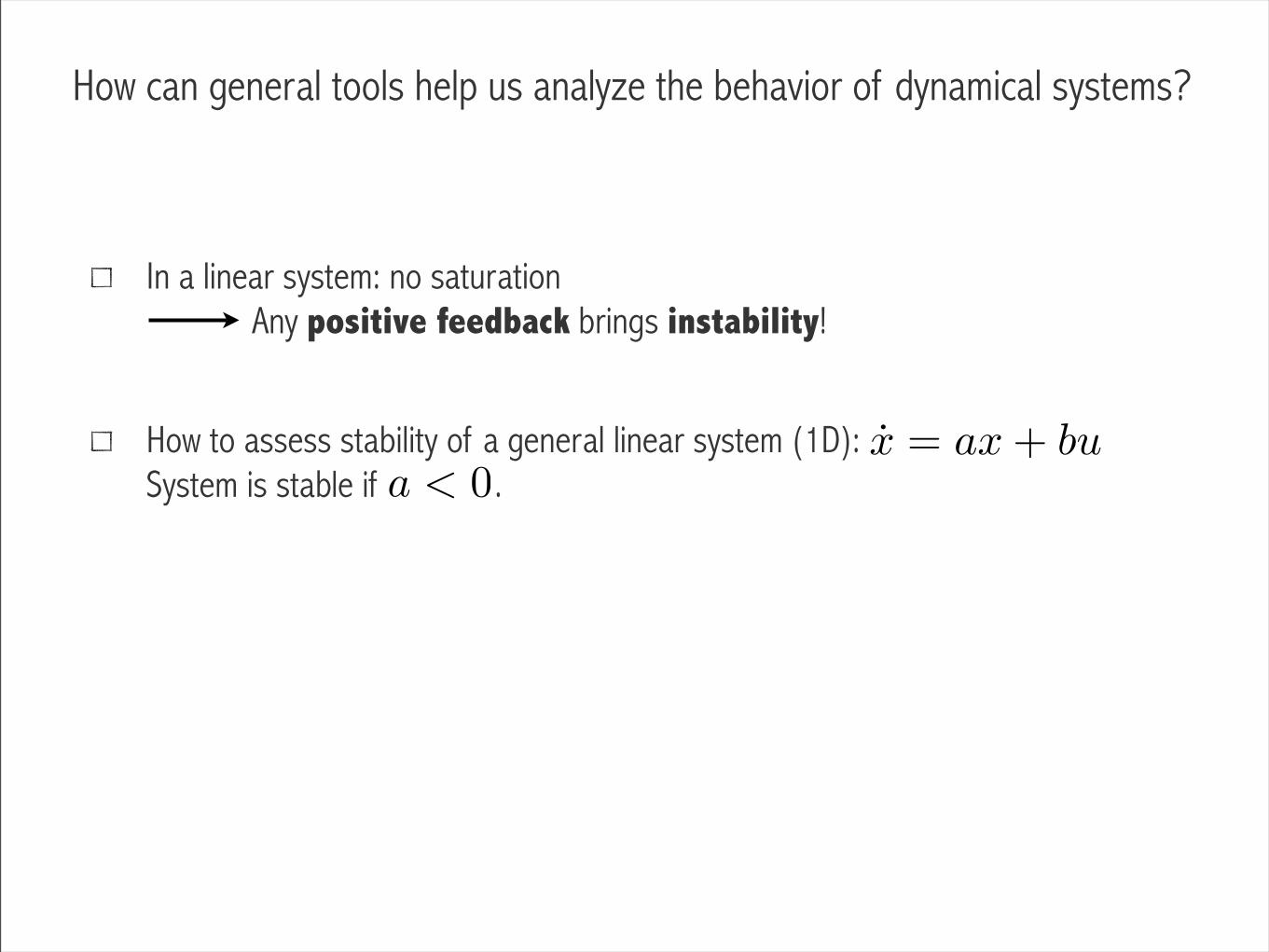
How can general tools help us analyze the behavior of dynamical systems?
In a linear system: no saturation Any positive feedback brings instability!
How to assess stability of a general linear system (1D):System is stable if .
a < 0x = ax+ bu

How can general tools help us analyze the behavior of dynamical systems?
In a linear system: no saturation Any positive feedback brings instability!
How to assess stability of a general linear system (1D):System is stable if .
How to assess stability of a general linear system (N-D): Multiple state-interactions: what are the feedbacks?N-feedback directions (eigenvectors of matrix ), each having its own amplitude(eigenvalues of ). The system is stable if (all feedbacks negative).
a < 0x = ax+ bu
x = Ax+Bu
R(eig(A)) < 0
AA
Outline
Inputs and outputs: signals
System dynamics: static gain, input integration and state interactions (feedback)
System output: update function vs output function
62