modeling and analysis of systems general informationsguilldrion/files/syst0002-2016-17... ·...
TRANSCRIPT

Modeling and Analysis of SystemsGeneral Informations
Guillaume DrionAcademic year 2016-2017
SYST0002 - General informations
Website: http://sites.google.com/site/gdrion25/teaching/syst0002
Contacts: Guillaume Drion - [email protected] Marie Wehenkel (teaching assistant) - [email protected]
Organization: 9 or 10 main lessons - Tuesday 10:45 to 12:45 9 tutorial sessions split in 4 groups - Monday 10:45 to 12:45 (rooms to be determined) - Thursday 8:30 to 10:30
Theory and exercises follow the textbooks provided on the website (in French).The textbooks are the same as last year!

Schedule of the year
Tutorials will start on Monday, October 4!

Goals of the course and evaluation
Goals of the course:
Lessons: intuition! The main goal of this course is to provide a general (and simple) framework for the analysis of possibly complex systems.
Tutorials: develop your technical skills, methods.
Evaluation:
Project: throughout the year (cut in pieces with several deadlines).
Exam: 2-3 questions to test your technical skills (tutorial style). 1-2 questions to test your basic knowledge and intuition.

Modeling and Analysis of SystemsLecture #1 - Introduction to Systems Theory
Guillaume DrionAcademic year 2016-2017

Modeling and analysis of systems
Real problems

Modeling and analysis of systems
Real problems
Engineering problems

Modeling and analysis of systems
Real problems
Engineering problems
SYSTEMS MODELING
AnalysisDesignImplementation
“Applied mathematics”

Modeling and analysis of systems
Historical example: mechanics before and after Newton.

Modeling and analysis of systems
Contemporary examples:
analysis and design of next generation materials (graphene).

Modeling and analysis of systems
Contemporary examples:
analysis and design of next generation materials (graphene).
engineering in life sciences (cardiovascular physiology, neuroscience).
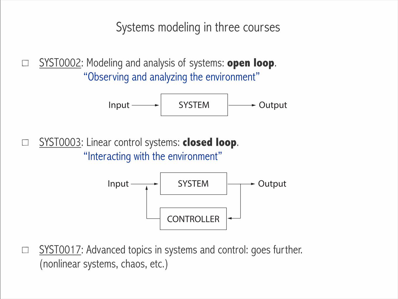
Systems modeling in three courses
SYST0002: Modeling and analysis of systems: open loop. “Observing and analyzing the environment”
SYST0003: Linear control systems: closed loop. “Interacting with the environment”
SYST0017: Advanced topics in systems and control: goes further. (nonlinear systems, chaos, etc.)
SYSTEMInput Output
SYSTEMInput Output
CONTROLLER

Modeling and analysis of systems
Systems theory:
translates a possibly complex problem in mathematics.
develops and uses specific set of tools to solve these problems.
more general/abstract = more powerful.

Modeling and analysis of systems
Illustration: what is the common point between a simple suspension, an electrical circuit and the mammalian cardiovascular system?

Modeling and analysis of systems
Illustration: what is the common point between a simple suspension, an electrical circuit and the mammalian cardiovascular system?
Answer: they all have very similar dynamical and input/output behaviors.

Modeling and analysis of systems
Illustration: what is the common point between a simple suspension, an electrical circuit and the mammalian cardiovascular system?
Answer: they all have very similar dynamical and input/output behaviors.
⌧ =m
B=
B
K
= RC =L
R
Stimulation ON Stimulation OFF
m = massB = dampingK = stiffness
R = resistanceC = capacitanceL = inductance
?
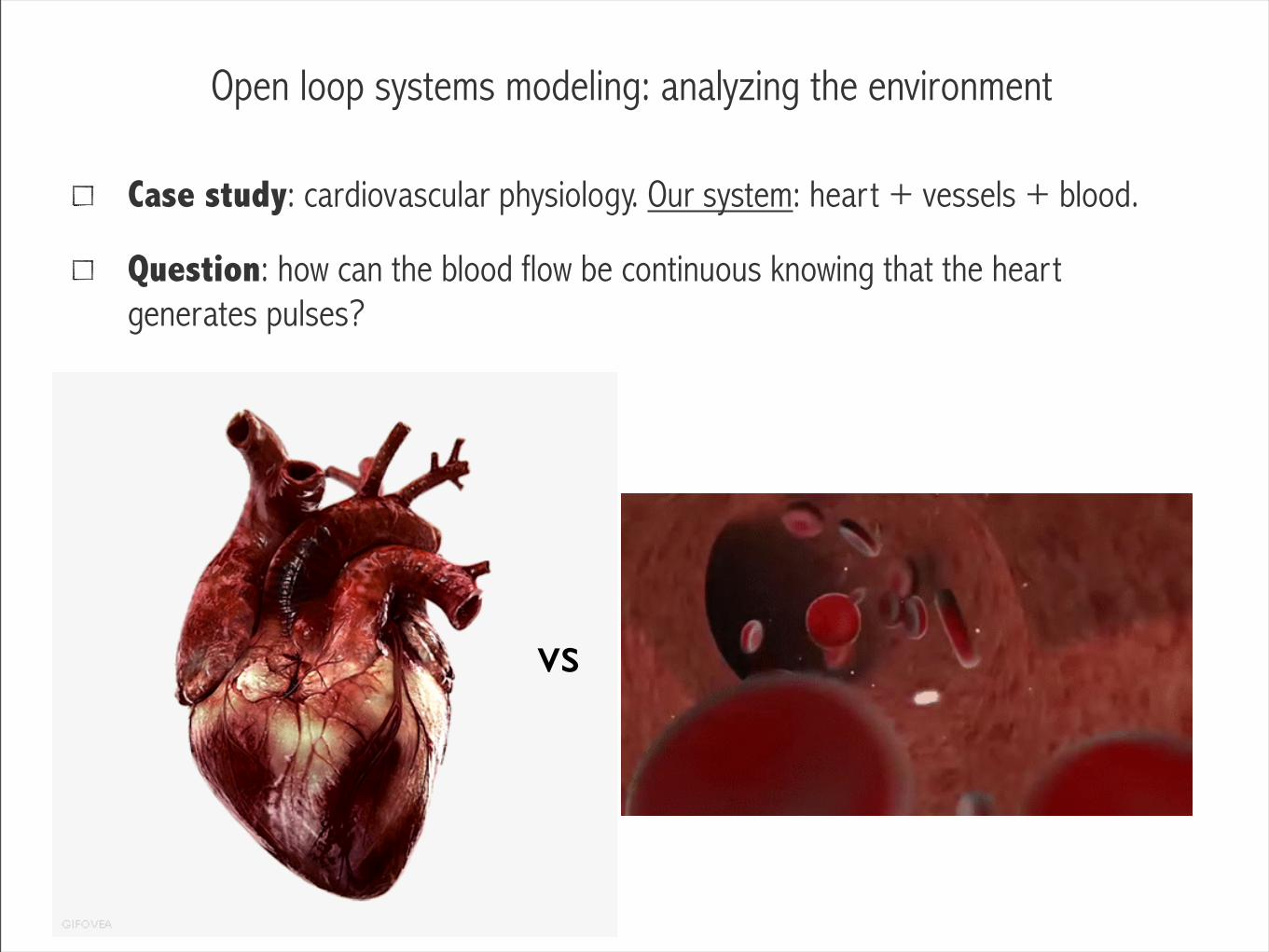
Open loop systems modeling: analyzing the environment
Case study: cardiovascular physiology. Our system: heart + vessels + blood.
Question: how can the blood flow be continuous knowing that the heart generates pulses?
vs

Modeling the cardiovascular system
Measurements: pressure in the left ventricle LV (input) and in the Aorta Ao(output).

Modeling the cardiovascular system
Measurements: pressure in the left ventricle LV (input) and in the Aorta Ao(output).
LV: large variations. Ao: stays highly positive (between 80 and 120 mmHg).
InputOutput
LV and Ao pressure variations over time are signals.

Modeling the cardiovascular system
Pathology: some patients have higher systolic pressure with lower diastolic pressure. Why? (It happens mostly in older patients).
Answering this question is very important because these patients are prone to heart failures. What can we do to “fix” the problem?

Modeling the cardiovascular system: Otto Frank.
In 1899, german physiologist Otto Frank came up with a first mathematical representation of the LV-Ao system: the Windkessel Model.
We will use this example to introduce the different ways to model a system
1. Find an equivalent representation of the system under study (Ch2, Ch3)
2. Put system into equations (Ordinary Differential Equations or Difference Equations)
• State-space representation (Ch2-3-4)
3. Extract system input/output properties (Laplace/Fourier or z-transform) (Ch 5-6)
• Transfer function (Ch7)
• System analysis (effects of changes in parameters?) (Ch8-9-10)
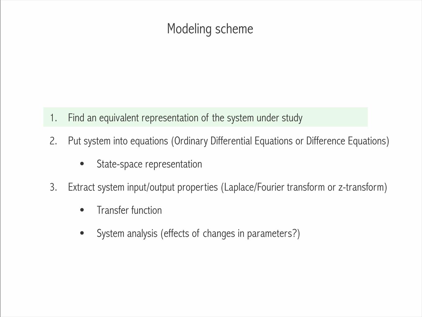
Modeling scheme
1. Find an equivalent representation of the system under study
2. Put system into equations (Ordinary Differential Equations or Difference Equations)
• State-space representation
3. Extract system input/output properties (Laplace/Fourier transform or z-transform)
• Transfer function
• System analysis (effects of changes in parameters?)

Find an equivalent representation of the system under study
Linear algebra
Matrix algebraDifference equations
Informatics
AlgorithmsProgramming
Numerical analysis
Numerical methodsOptimization
Mathematical analysis
Ordinary differential equationsSeriesFourier transformConvolution
Physics
Laws of mechanicsLaws of electricity and electromagnetism
Chemistry
Chemical reactionsOrganic chemistryThermodynamics

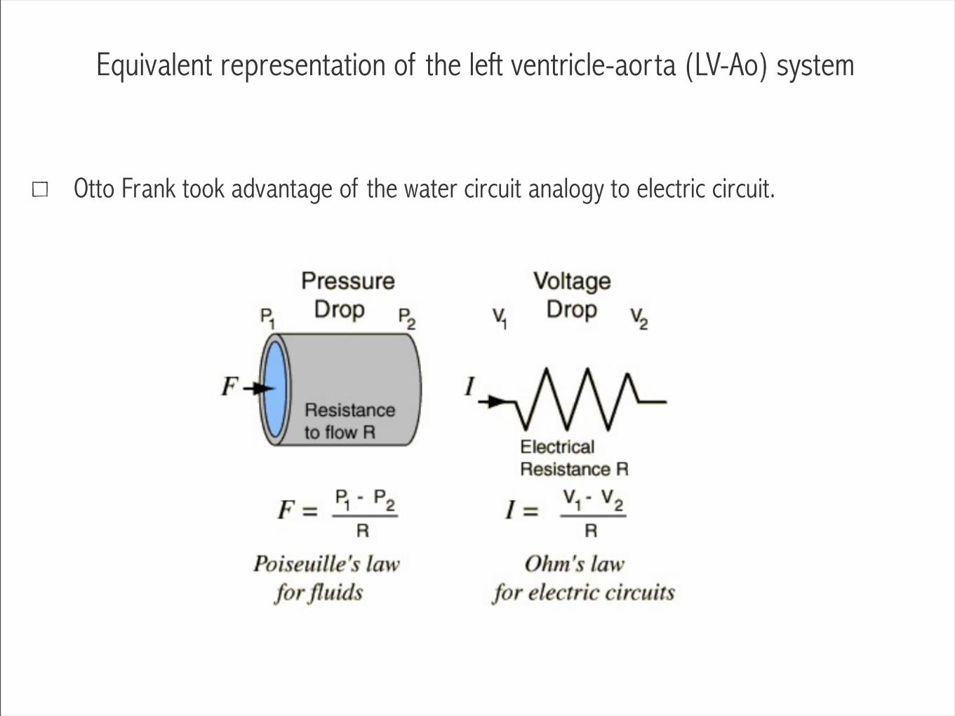
Equivalent representation of the left ventricle-aorta (LV-Ao) system
Otto Frank took advantage of the water circuit analogy to electric circuit.
Left ventricle
Aortic valve (r)
Aorta
Arterial compliance (Ca)
Peripheryvessels
(R1, R2, ..., Rn)
r
RCaP(t)
u(t)
PCa(t)Pr(t)
Equivalent representation of the left ventricle-aorta (LV-Ao) system
Otto Frank took advantage of the water circuit analogy to electric circuit.

Left ventricle
Aortic valve (r)
Aorta
Arterial compliance (Ca)
Peripheryvessels
(R1, R2, ..., Rn)
r
RCaP(t)
u(t)
PCa(t)Pr(t)
The 3-Element Windkessel model - Circuit diagram
1. Equivalent circuit of the LV-Ao system
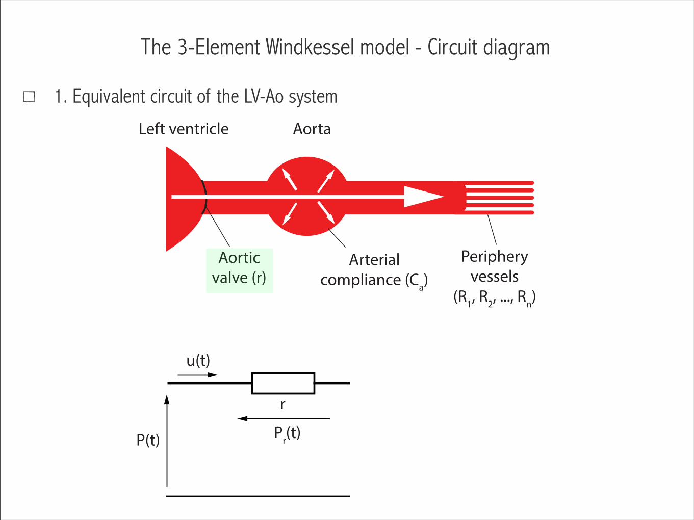
Left ventricle
Aortic valve (r)
Aorta
Arterial compliance (Ca)
Peripheryvessels
(R1, R2, ..., Rn)
r
RCaP(t)
u(t)
PCa(t)Pr(t)
The 3-Element Windkessel model - Circuit diagram
1. Equivalent circuit of the LV-Ao system
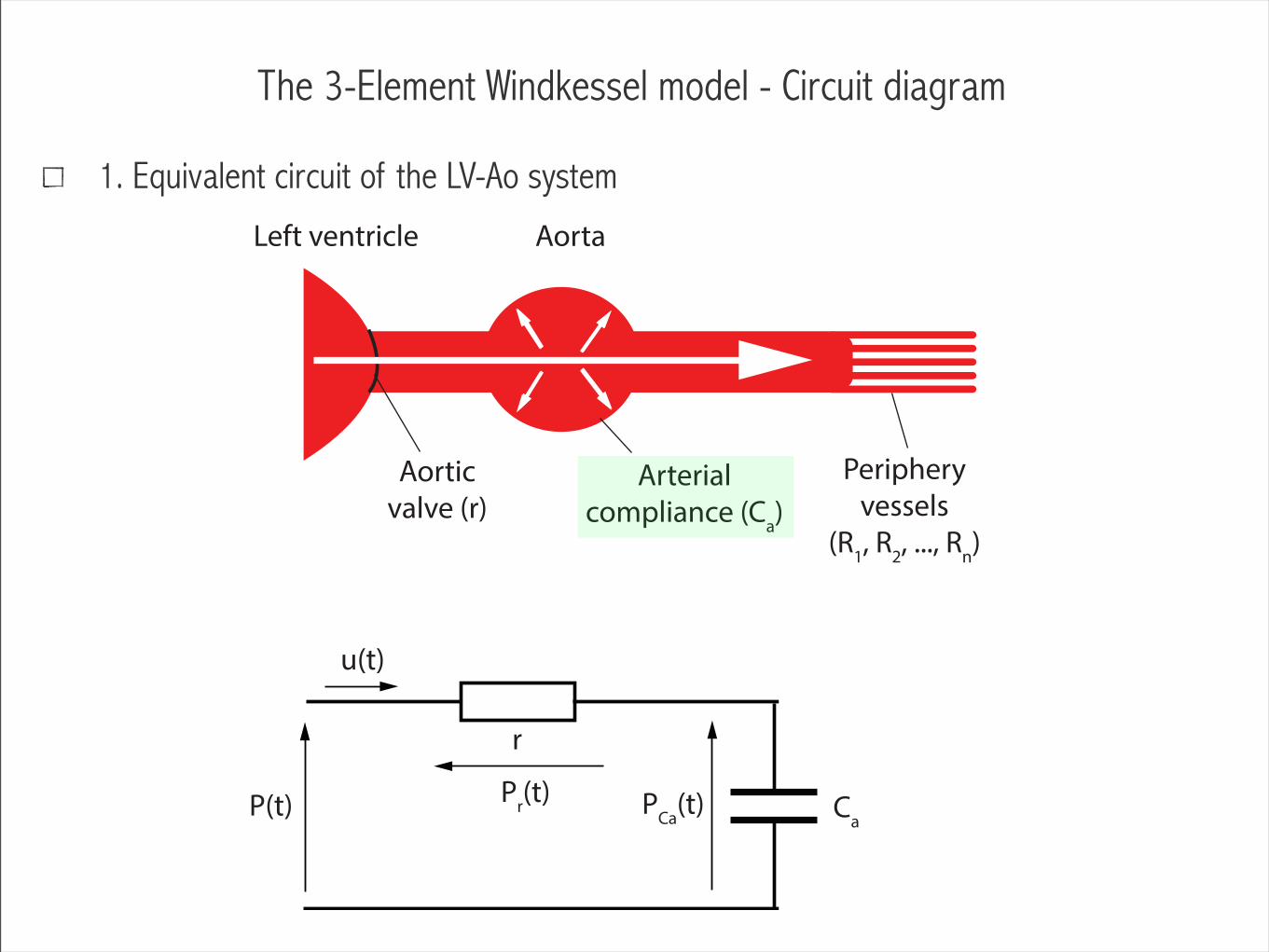
Left ventricle
Aortic valve (r)
Aorta
Arterial compliance (Ca)
Peripheryvessels
(R1, R2, ..., Rn)
r
RCaP(t)
u(t)
PCa(t)Pr(t)
The 3-Element Windkessel model - Circuit diagram
1. Equivalent circuit of the LV-Ao system

Left ventricle
Aortic valve (r)
Aorta
Arterial compliance (Ca)
Peripheryvessels
(R1, R2, ..., Rn)
r
RCaP(t)
u(t)
PCa(t)Pr(t)
The 3-Element Windkessel model - Circuit diagram
1. Equivalent circuit of the LV-Ao system

r
RCaP(t)
u(t)
PCa(t)Pr(t)
The 3-Element Windkessel model - Circuit diagram
1. Equivalent circuit of the LV-Ao system

Modeling scheme
1. Find an equivalent representation of the system under study
2. Put system into equations (Ordinary Differential Equations or Difference Equations)
• State-space representation
3. Extract system input/output properties (Laplace/Fourier transform or z-transform)
• Transfer function
• System analysis (effects of changes in parameters?)

The 3-Element Windkessel model - Circuit diagram
2. Mathematical description of the dynamical system: ordinary differential equations
r
RCaP(t)
u(t)
PCa(t)Pr(t)

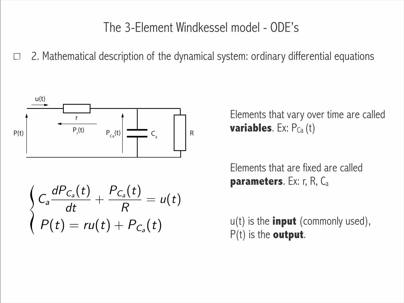
The 3-Element Windkessel model - ODE’s
2. Mathematical description of the dynamical system: ordinary differential equations
Kirchhoff’s voltage law:
r
RCaP(t)
u(t)
PCa(t)Pr(t)
P(t) = Pr (t) + PCa(t) = ru(t) + PCa
(t)

The 3-Element Windkessel model - ODE’s
2. Mathematical description of the dynamical system: ordinary differential equations
Kirchhoff’s current law:
Kirchhoff’s voltage law:
r
RCaP(t)
u(t)
PCa(t)Pr(t)
P(t) = Pr (t) + PCa(t) = ru(t) + PCa
(t)
u(t) = iCa(t) + ir (t) = Ca
dPCa(t)
dt+
PCa(t)
R

The 3-Element Windkessel model - ODE’s
2. Mathematical description of the dynamical system: ordinary differential equations
r
RCaP(t)
u(t)
PCa(t)Pr(t)
P(t) = ru(t) + PCa(t)
Ca
dPCa(t)
dt+
PCa(t)
R= u(t)
The 3-Element Windkessel model - ODE’s
r
RCaP(t)
u(t)
PCa(t)Pr(t)
P(t) = ru(t) + PCa(t)
Ca
dPCa(t)
dt+
PCa(t)
R= u(t)
2. Mathematical description of the dynamical system: ordinary differential equations
Elements that vary over time are called variables. Ex: PCa (t)
Elements that are fixed are called parameters. Ex: r, R, Ca
u(t) is the input (commonly used),P(t) is the output.

The 3-Element Windkessel model - Simulation
2A. Validation of the model: simulation (ex: matlab)
u(t)
P(t)
r
RCaP(t)
u(t)
PCa(t)Pr(t)
P(t) = ru(t) + PCa(t)
Ca
dPCa(t)
dt+
PCa(t)
R= u(t)

The 3-Element Windkessel model - State-space
2B. State-space canonical representation
Linear, time-invariant (LTI) dynamical systems can be represented in the form
y = Cx + Du
x = Ax + Bu
where A is the dynamics matrix,
B is the input matrix,
C the output matrix,
D the feedthrough matrix.
Linear: the output is a linear function of the input (not y = x2 for instance)
Time-invariant: parameters do not change over time. (A, B, C and D does not depend on time). Here: the values of r, R and Ca are fixed.

The 3-Element Windkessel model - State-space
2B. State-space canonical representation
y = Cx + Du
x = Ax + Bu
where A is the dynamics matrix,
B is the input matrix,
C the output matrix,
D the feedthrough matrix.
P(t) = PCa(t) + ru(t)
dPCa(t)
dt= −
1
RCa
PCa(t) +
1
Ca
u(t)
Linear, time-invariant (LTI) dynamical systems can be represented in the form
Linear: the output is a linear function of the input (not y = x2 for instance)
Time-invariant: parameters do not change over time. (A, B, C and D does not depend on time). Here: the values of r, R and Ca are fixed.

The 3-Element Windkessel model - State-space
2B. State-space canonical representation
y = Cx + Du
x = Ax + Bu
where A is the dynamics matrix,
B is the input matrix,
C the output matrix,
D the feedthrough matrix.
P(t) = PCa(t) + ru(t)
x(t) = PCa(t), y(t) = P(t)
A = −
1
RCa
,B =1
Ca
,C = 1,D = r
dPCa(t)
dt= −
1
RCa
PCa(t) +
1
Ca
u(t)
Linear, time-invariant (LTI) dynamical systems can be represented in the form
Linear: the output is a linear function of the input (not y = x2 for instance)
Time-invariant: parameters do not change over time. (A, B, C and D does not depend on time). Here: the values of r, R and Ca are fixed.

The 3-Element Windkessel model - State-space
A - the dynamics matrix (“states feed back on themselves”)
y = Cx + Du
x = Ax + Bu x(t) = PCa(t), y(t) = P(t)
A = −
1
RCa
,B =1
Ca
,C = 1,D = r
u is the input of the system, y is the output. What is x?
x is called a state. A state describes the internal dynamics of the system.Hence the name state-space representation.
The matrix A describes how the states influence themselves (x = Ax), and therefore describes how the dynamics of the system evolve (dynamics matrix).

The 3-Element Windkessel model - State-space
B - the input matrix
y = Cx + Du
x = Ax + Bu x(t) = PCa(t), y(t) = P(t)
A = −
1
RCa
,B =1
Ca
,C = 1,D = r
The input not only directly affects the output of the system, but also affects the internal states.
The matrix B describes how the input influences the states (x = Bu) (input matrix).

The 3-Element Windkessel model - State-space
C - the output matrix
y = Cx + Du
x = Ax + Bu x(t) = PCa(t), y(t) = P(t)
A = −
1
RCa
,B =1
Ca
,C = 1,D = r
The output of a system is mostly shaped by its internal states.
The matrix C describes how the states are seen in the output (y = Cx) (output matrix).

The 3-Element Windkessel model - State-space
D - the feedthrough matrix
y = Cx + Du
x = Ax + Bu x(t) = PCa(t), y(t) = P(t)
A = −
1
RCa
,B =1
Ca
,C = 1,D = r
Some part of the input might also affect the output without “being affected” by the dynamics of the system.
The matrix D describes how the input directly influences the output (y = Du) (feedthrough matrix).
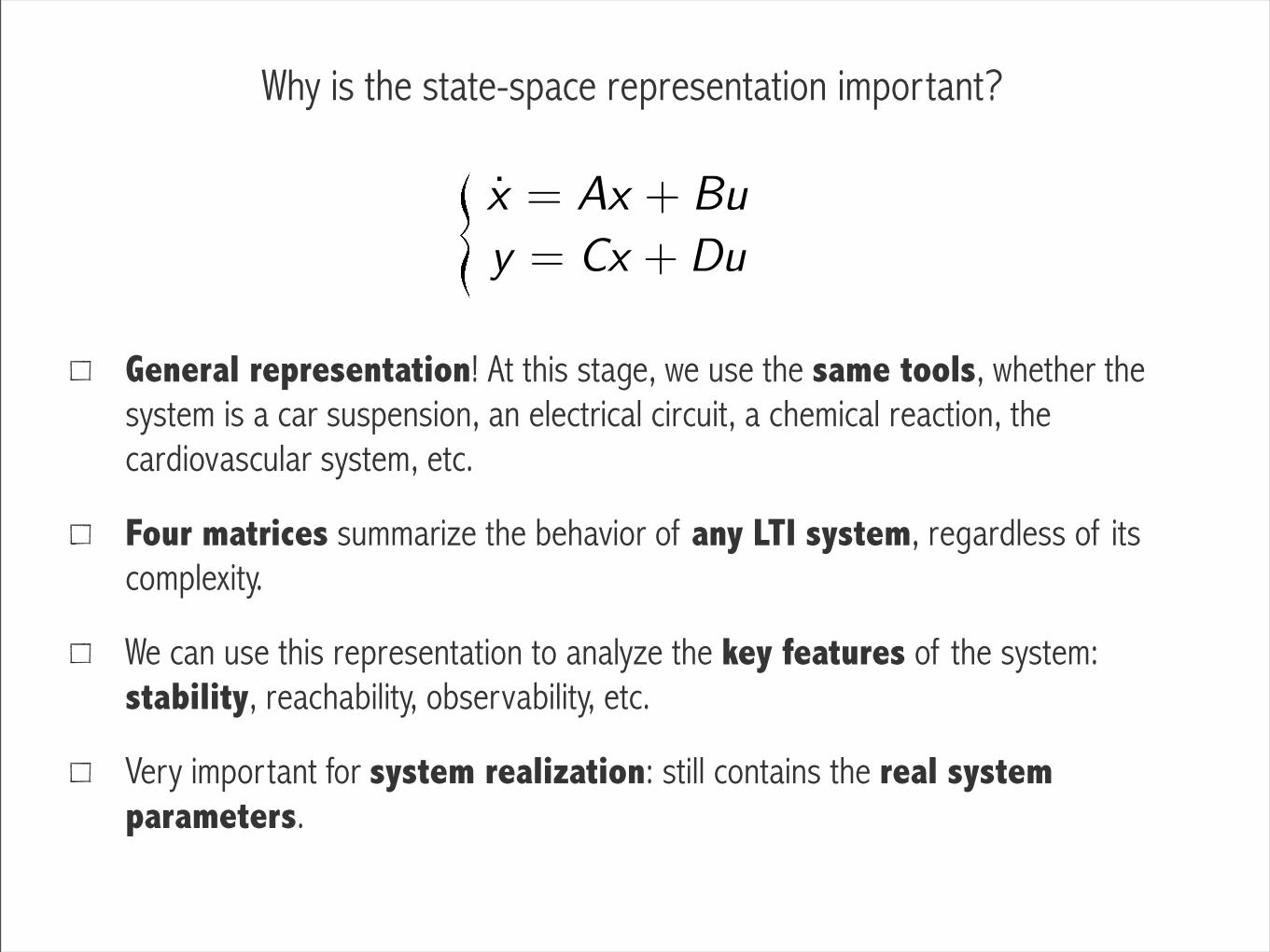
Why is the state-space representation important?
General representation! At this stage, we use the same tools, whether the system is a car suspension, an electrical circuit, a chemical reaction, the cardiovascular system, etc.
Four matrices summarize the behavior of any LTI system, regardless of its complexity.
We can use this representation to analyze the key features of the system: stability, reachability, observability, etc.
Very important for system realization: still contains the real system parameters.
y = Cx + Du
x = Ax + Bu

Back to our case study
Questions:
How can the blood flow be continuous knowing that the heart generates pulses?
Some patients have higher systolic pressure with lower diastolic pressure. Why?
y = Cx + Du
x = Ax + Bu x(t) = PCa(t), y(t) = P(t)
A = −
1
RCa
,B =1
Ca
,C = 1,D = r

Modeling scheme
1. Find an equivalent representation of the system under study
2. Put system into equations (Ordinary Differential Equations or Difference Equations)
• State-space representation
3. Extract system input/output properties (Laplace/Fourier transform or z-transform)
• Transfer function
• System analysis (effects of changes in parameters?)

Frequency domain: introduction
You have seen the Fourier transform in calculus.
In this course, we will use the Fourier transform, and others such as the Laplace transform (continuous time) and z-transform (discrete time) to move from the time domain to the frequency domain.
where ω is an angular frequency (rad/s).

Frequency domain: introduction
The idea is to decompose a signal into the frequencies that compose it and analyze how a system transmit/transform these frequencies.

Frequency domain: introduction
The idea is to decompose a signal into the frequencies that compose it and analyze how a system transmit/transform these frequencies.

Frequency domain: introduction
The idea is to decompose a signal into the frequencies that compose it and analyze how a system transmit/transform these frequencies.

Frequency domain: introduction
The idea is to decompose a signal into the frequencies that compose it and analyze how a system transmit/transform these frequencies.
Low frequency High frequency

Frequency domain: Fourier transform vs Laplace transform
Fourier transform
where ω is an angular frequency (rad/s).
Laplace transform
where s is the complex frequency s = σ + jω.

Why working in the frequency domain?
Many advantages, here is one of them:
Time domain Frequency domain

The 3-Element Windkessel model - Transfer function
3. Input/output properties: transfer function (frequency domain via Laplace transform)
Idea: describe the system through a simple function that characterizes the way it affects an input U(s)
“s” is the complex number frequency (s = σ+jω). If σ=0: Fourier transform!
U(s) H(s) Y(s) and

The 3-Element Windkessel model - Transfer function
3. Input/output properties: transfer function (frequency domain via Laplace transform)
U(s) H(s) Y(s)
Idea: describe the system through a simple function that characterizes the way it affects an input U(s)
“s” is the complex number frequency (s = σ+jω). If σ=0: Fourier transform!
There are different ways to compute the transfer function of a system. However, it is convenient to start from the canonical state-space representation (if available)
y = Cx + Du
x = Ax + Bu
which gives
H(s) =Y (s)
U(s)= C (sI − A)−1
B + D (see next slide)
and
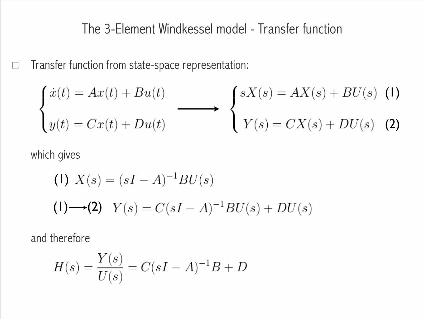
The 3-Element Windkessel model - Transfer function
Transfer function from state-space representation:
which gives
and therefore
(1)
(2)
(1)
(1) (2)

The 3-Element Windkessel model - Transfer function
3. Input/output properties: transfer function (frequency domain via Laplace transform)
Transfer function of the 3-Element Windkessel model ( )
H(s) =Y (s)
U(s)= C (sI − A)−1
B + D
A = −
1
RCa
,B =1
Ca
,C = 1,D = r

The 3-Element Windkessel model - Transfer function
H(s) =Y (s)
U(s)= C (sI − A)−1
B + D
3. Input/output properties: transfer function (frequency domain via Laplace transform)
Transfer function of the 3-Element Windkessel model ( )A = −
1
RCa
,B =1
Ca
,C = 1,D = r
= 1(s +1
RCa
)−11
Ca
+ r

The 3-Element Windkessel model - Transfer function
H(s) =Y (s)
U(s)= C (sI − A)−1
B + D
3. Input/output properties: transfer function (frequency domain via Laplace transform)
Transfer function of the 3-Element Windkessel model ( )A = −
1
RCa
,B =1
Ca
,C = 1,D = r
= 1(s +1
RCa
)−11
Ca
+ r
=R
RCas + 1+ r

The 3-Element Windkessel model - Transfer function
H(s) =Y (s)
U(s)= C (sI − A)−1
B + D
≡
K
τs + 1+ r => Low pass filter! (r<< physiologically)
K=R: gain τ=RCa: time constant ωc=1/τ: cutoff frequency
3. Input/output properties: transfer function (frequency domain via Laplace transform)
Transfer function of the 3-Element Windkessel model ( )A = −
1
RCa
,B =1
Ca
,C = 1,D = r
=R
RCas + 1+ r
= 1(s +1
RCa
)−11
Ca
+ r

The 3-Element Windkessel model - Transfer function
≡
K
τs + 1+ rLow-pass filter

The transfer function of the Windkessel model helps making predictions on the potential effects of physiological and/or pathological conditions on blood pressure
Low frequency High frequency
Low pass filter
τ = RCa
H(s) =R
RCas + 1+ r

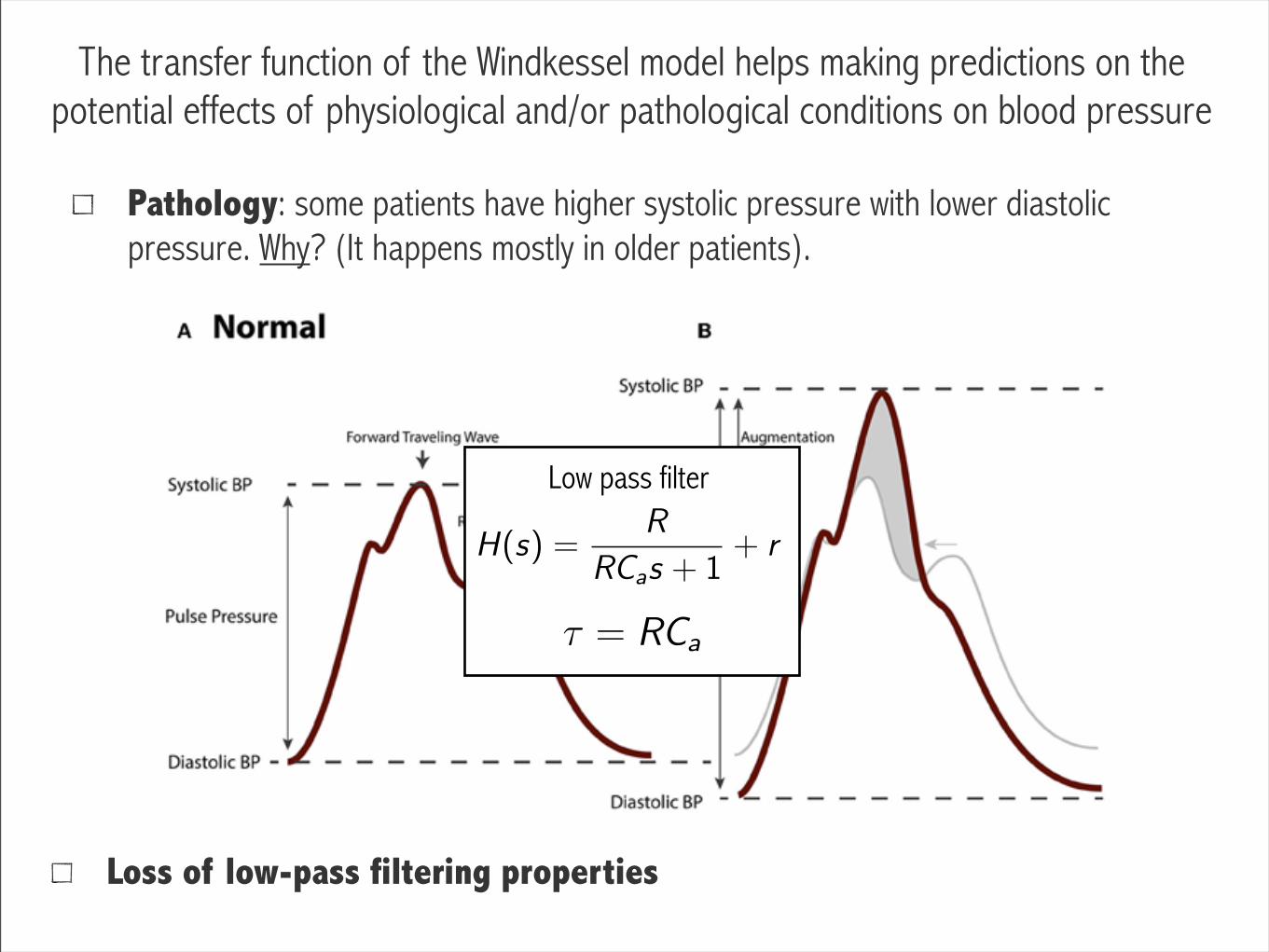
The transfer function of the Windkessel model helps making predictions on the potential effects of physiological and/or pathological conditions on blood pressure
Pathology: some patients have higher systolic pressure with lower diastolic pressure. Why? (It happens mostly in older patients).

The transfer function of the Windkessel model helps making predictions on the potential effects of physiological and/or pathological conditions on blood pressure
Pathology: some patients have higher systolic pressure with lower diastolic pressure. Why? (It happens mostly in older patients).
Loss of low-pass filtering properties
Low pass filter
τ = RCa
H(s) =R
RCas + 1+ r

The transfer function of the Windkessel model helps making predictions on the potential effects of physiological and/or pathological conditions on blood pressure
Atherosclerosis: loss of arterial compliance => Ca decreases => τ=RCa decreases
τ = RCa
Low pass filter
H(s) =R
RCas + 1+ r

Modeling the cardiovascular system: conclusion
The vascular system acts as a low-pass filter, following slow heart movements but filtering fast heart movements.
This allows to maintain a rather constant blood flow in the system.
InputOutput

Modeling scheme
1. Find an equivalent representation of the system under study
2. Put system into equations (Ordinary Differential Equations or Difference Equations)
• State-space representation
3. Extract system input/output properties (Laplace/Fourier transform or z-transform)
• Transfer function
• System analysis (effects of changes in parameters?)