modeling air traffic management technologies with a ... · modeling air traffic management...

NASA / CR- 1999- 208988

Modeling Air Traffic Management

Technologies With a Queuing Network

Model of the National Airspace System

Dou Long, David Lee, Jesse Johnson, Eric Gaier, and Peter Kostiuk

Logistics Management Institute, McLean, Virginia

National Aeronautics and

Space Administration

Langley Research Center

Hampton, Virginia 23681-2199

Prepared for Langley Research Centerunder Contract NAS2-14361

January 1999 : .

https://ntrs.nasa.gov/search.jsp?R=19990024952 2018-07-05T01:10:37+00:00Z

Available from:

NASA Center for AeroSpace Information (CASt)7121 Standard Drive

Hanover, MD 21076-1320

(301) 621-0390

National Technical Information Service (NTIS)

5285 Port Royal Road

Springfield, VA 22161-2171(703) 605-6000

Contents

Chapter 1 Overview ........................................................................................... 1-1

Chapter 2 LMINET ........................................................................................... 2-1

AIRPORT DELAY MODEL ................................................................................................... 2-2

Arrival Service Process .............................................................................................. 2-3

Taxi-Delay Queues ..................................................................................................... 2-4

Departure Service Processes ...................................................................................... 2-6

Equations of the Extended Airport Delay Model ....................................................... 2-6

Calibrating the Airport Delay Model ......................................................................... 2-9

An Example of the LMINET Airport Delay Model ................................................. 2-11

Effect of Night-Time Taxi Speeds ........................................................................... 2-12

AIRPORT CAPACITY MODEL ............................................................................................ 2-13

Arrivals Only ............................................................................................................ 2-15

Sequences of Alternating Arrivals and Departures .................................................. 2-19

Statistics of Multiple Operations .............................................................................. 2-20

Input-Stream Effects ................................................................................................. 2-26

Completing the Pareto Frontier of Runway Capacity .............................................. 2-27

MODELS OF TRACON AND ARTCC SECTORS ............................................................... 2-28

M/E3/N/N+Q Sector Model ...................................................................................... 2-28

TRACON Models .................................................................................................... 2-31

En Route Sector Models ........................................................................................... 2-31

Automatic Traffic Flow Controller .......................................................................... 2-31

Chapter 3 Adjusting LMINET to Model the NAS ............................................ 3-1

DEMAND INPUTS ............................................................................................................... 3-1

Demand in 1996 ......................................................................................................... 3-1

Demand in 2007 ......................................................................................................... 3-2

CAPACITY MODELS ............................................................................................................ 3-8

Airport Airside Capacity Models ............................................................................... 3-9

nl

Airport Surface-Delay Model ................................................................................... 3-10

Chapter 4 Modeling IndividualATM Technologies ......................................... 4-1

MODELING TAP TECHNOLOGmS ....................................................................................... 4-1

Dynamic Runway Occupancy Measurement .............................................................. 4-1

Roll Out and Turn Off ................................................................................................ 4-1

Aircraft Vortex Spacing System ................................................................................. 4-1

ATM 4-2

T-NASA ..................................................................................................................... 4-2

MODELING NASA AATT TECHNOLOGmS ........................................................................ 4-2

General Considerations for Modeling DSTs .............................................................. 4-2

TMA, P-FAST, and A-FAST ..................................................................................... 4-3

En Route and Descent Advisor .................................................................................. 4-6

Expedite Departure Path ........................................................................................... 4-10

National Surface Movement Tool ............................................................................ 4-11

E-CDTI and APATH ................................................................................................ 4-13

Chapter 5 ATM Impacts on Network Parameters ............................................. 5-1

TOOLS MODELED AND NOT MODELED .............................................................................. 5-1

LEVELS OF CONFIDENCE IN THE PARAMETRIC MODELS ...................................................... 5-3

TABLE OF MODELING PARAMETERS .................................................................................. 5-4

Airport Parameters ..................................................................................................... 5-4

TRACON Parameters ................................................................................................. 5-5

ARTCC Parameters .................................................................................................... 5-7

FOUR SPECIFIC CASES ....................................................................................................... 5-7

2007 Reference ........................................................................................................... 5-7

All TAP and AATT .................................................................................................... 5-7

TAP Only ................................................................................................................... 5-8

AATT Only ................................................................................................................ 5-8

Chapter 6 Impacts of ATM Technologies on NAS Operations ........................ 6-1

Chapter 7 Economic Impacts of ATM Technologies ....................................... 7-1

MODEL STRUCTURE ................................................................................ . ......................... 7-1

iv

Contents

VOC VERSUS DOC .......................................................... . ............................................... 7-2

CALCULATION OF DELAY COSTS ....................................................................................... 7-3

COMPOSrrE ANALYSIS ....................................................................................................... 7-6

SUMMARY ......................................................................................................................... 7-9

Chapter 8 Delay Impact on System Throughput ............................................... 8-1

Am CARRIER INVESTMENT MODEL ................................................................................... 8-2

USING THE ACIM TO EVALUATE CHANGES IN SYSTEM THROUGHPUT .............................. 8-3

ACIM THROUGI-IPtrr RESULTS .......................................................................................... 8-6

EXTENDING THE RESULTS TO COMMIYrER AND GA TRAFFIC ............................................ 8-9

Chapter 9 Summary and Conclusions ............................................................... 9-1

Appendix A 1996 Variable Operating Costs For the U.S. Fleet ..................... A-1

Appendix B A First-Moment Closure Hypothesis for M/EJ1 Queues ........... B-1

Appendix C Glossary of Airport Identifiers .................................................... C- 1

FIGURES

Figure

Figure

Figure

Figure

Figure

Figure

Figure

Figure

Figure

Figure

Figure

Figure

Figure

Figure

2-1.

2-2.

2-3.

2-4.

2-5.

2-6.

2-7.

2-8.

LMINET Airports ................................................................................................ 2-1

Queues in the LMINET Airport Model ............................................................... 2-2

Some Erlang Distributions ................................................................................... 2-4

Comparison of Service-Time (Interarrival Time) Distributions ........................ 2-10

Calibration of Surface-Delay Model .................................................................. 2-11

Example Runway Capacity ................................................................................ 2-14

Flight Trajectories, Gaining Follower ............................................................... 2-15

Hight Trajectories, Lagging Follower ............................................................... 2-18

2-9. Flight Trajectories, Mixed Arrival and Departure ............................................. 2-20

2-10. Example Probability Distribution of Interarrival Time ................................... 2-22

2-11. Distribution Function of the Time for Two Arrivals ....................................... 2-25

2-12. Distribution of the Time for Four Arrivals ...................................................... 2-25

2-13. Example Interarrival Distribution with Input-Stream Effects ......................... 2-27

3-1. Total LMINET Airport Annual Operations (millions) ........................................ 3-5

V

Figure 3-2. Total LMINET Airport Annual Enplanements (millions) ................................... 3-6

Figure 4-I. Capacity Comparisons ......................................................................................... 4-6

Figure 4-2. Variation of Controller Utilization with Maximum Number of Aircraft in

Sector ................................................................................................................................ 4-9

Figure 4-3. Smoothed Sample PDF of Mean Taxi-in Delay Times at the 64 LMINET

Airports ........................................................................................................................... 4-13

Figure 6-1. Total Annual Delays in Aircraft-Minutes ............................................................ 6-1

Figure

Figure

Figure

Figure

Figure

Figure

Figure

Figure

Figure

Figure

Figure

6-2.

6-3.

6-4.

Arrival Queues at ATL ........................................................................................ 6-3

Ground-Hold Queues at ATL .............................................................................. 6-4

Arrival Queues at ORD ............... .,,,., .................................................................. 6-5

6-5. Ground-Hold Queues At ORD ............................................................................ 6-5

7-I. Schematic Diagram of Overall Cost Structure .................................................... 7-2

7-2. Annual Cross Comparable Benefits .................................................................... 7-8

8-1. Arrival Demand and Capacity at DCA ........... ..................................................... 8-1

8-2. FCM Schematic ................................................................................................... 8-3

8-3: Schematic of ACIM Approach ............................................................................ 8-4

8-4: Commercial Operations ....................................................................................... 8-9

B-1. Comparison of Exact and Closure-Hypothesis Results for <n> ........................ B-2

TABLES

Table 2-1. LMINET Output For BOS, April 8, 1996 ........................................................... 2-12

Table 3-1. Annual Operations (thousands) and Enplanements (millions) at LMINET

Airports ............................................................................................................................. 3-3

Table 3-2. LMINET Airports Versus the Network (operations) ............................................ 3-4

Table 3-3. LMINET Airports Versus the Network (enplanements) ....................................... 3-5

Table 5-1. Miles-in-Trail Minima .......................................................................................... 5-6

Table 5-2. LMINET Parameters Modeling TAP and DST Tools and Combinations ofTools ................................................................................................................................. 5-9

Table 5-3. Parameters For Cases in Preliminary Report ...... . ............................................... 5-11

Table 6-1. LMINET Output for BOS, 2007 Baseline ............................................................ 6-6

Table 6-2. LMINET Output For BOS, TAP and AATT Technologies In Place .................... 6-7

Table 7-1. GA and Non-GA Combined Variable Operating Cost Calculation ...................... 7-4

vi

Contents

Table 7-2. Total Delay Cost Drivers in 1996 Dollars ............................................................ 7-4

Table 7-3. Yearly Block Minute Delay Costs in 1996 Dollars .............................................. 7-5

Table 7-4. Case Summary ...................................................................................................... 745

Table 7-5. Comparative Analysis ........................................................................................... 7-7

Table 7-6. Yearly Delay ($ billion) in 1996 Dollars .............................................................. 7-8

Table 8-1. FCM Delay Inputs ................................................................................................. 8-4

Table 8-2. Commercial RPM Results (billions) ..................................................................... 8-7

Table 8-3. Commercial Enplanement Results (millions) ....................................................... 8-7

Table A-1. 1996 Variable Operating Costs for the U.S. Fleet .............................................. A-1

vii

Chapter 1

Overview

This report describes an integrated model of air traffic management (ATM) tools

under development in two National Aeronautics and Space Administration

(NASA) programs--Terminal Area Productivity (TAP) and Advanced Air Trans-

port Technologies (AATT). The model is made by adjusting parameters of

LMINET, a queuing network model of the National Airspace System (NAS),

which the Logistics Management Institute (LMI) developed for NASA. Operating

LMINET with models of various combinations of TAP and AATT will give

quantitative information about the effects of the tools on operations of the NAS.

An extension of economic models developed by the Institute for NASA maps the

technologies' impacts on NAS operations into cross-comparable benefits esti-

mates for technologies and sets of technologies. An application of the Aviation

Systems Analysis Capability (ASAC) Air Carder Investment Model (ACIM), de-

veloped for NASA by the Institute, gives estimates of the ways in which the

NASA tools impact NAS throughput, as measured by revenue passenger miles

(RPMs), enplanements, and operations.

Following this overview chapter, Chapter 2 describes LMINET and its constituent

models in some detail. This information will help readers unfamiliar with

LMINET to understand ATM models made with LMINET parameters. For com-

pleteness, we have included in this report material from three other reports and an

LMI white paper, all of which were prepared for NASA by the Institute. [1,2,3,4]

Those familiar with LMINET's components need only consider the material in the

sections "Input-Stream Effects" and "Taxi-Delay Queues" in Chapter 2. The fn'st

describes a new LMINET parameter, developed to account for the fact that termi-

nal radar approach control (TRACON) controllers may present airport controllers

with arrival streams that are difficult to manage efficiently. The second explains

the model of taxiway delays that we have developed for this project.

Chapters 3 and 4 and describe, respectively, our models of two reference cases of

the NAS and of the TAP and AATT technologies. Chapter 5 summarizes our

modeling work. Chapter 6 summarizes the technologies' impacts on some aspects

of NAS operation. Chapter 7 summarizes the technologies' economic impacts.

Chapter 8 describes our means of estimating the impacts of delay on system

throughput and gives the throughput results. The report concludes with a summary

of principal results, given in Chapter 9.

1-1

fi| _t-'

Chapter 2

LMINET

Our principal tool for this study is LMINET, a queueing network model of the

NAS, developed by LMI for NASA. [1,3] Presently, LMINET is implemented

with 64 airports (Figure 2-1). _ They account for over 80 percent of the air carrier

operations for 1997, as reported in Department of Transportation (DOT)

Forms T-100. The LMINET airports are a superset of the Federal Aviation Ad-

ministration's (FAA's) 57 pacing airports.

Figure 2-1. LMINET Airports

In general terms, LMINET models flights among a set of airports by linking

queueing network models of airports with sequences of queuing models of

TRACON and Air Route Traffic Control Center (ARTCC) sectors. The user may

specify the sequences of sectors to represent various operating modes for the

1The 64 airports (denoted by three-letter codes) are ABQ, ATL, AUS, BDL, BNA, BOS,BUR, BWI, CLE, CLT, CMH, CVG, DAL, DAY, DCA, DEN, DFW, DTW, ELP, EWR, FLL,GSO, HOU, HPN, IAD, IAH, IND, ISP, JFK, LAS, LAX, LGA, LGB, MCI, MCO, MDW, MEM,MIA, MKE, MSP, MSY, OAK, ONT, ORD, PBI, PDX, PHL, PHX, PIT, RDU, RNO, SAN, SAT,SDF, SEA, SFO, SJC, SLC, SMF, SNA, STL, SYR, TEB, and TPA.

2-1

NAS. The sequences may, for example, correspond to optimal routes for the

winds aloft of a specific day or to trajectories of flights as flown on a specific day

as determined from data in the FAA's Enhanced Traffic Management System

(ETMS).

Given the sector sequences for the interairport routes, LMINET is driven by two

inputs: traffic demand and weather data. Traffic demand is input by a schedule of

hour-by-hour departures from the network airports and a schedule of arrivals to

network airports from terminals outside the network. The 1997 Official Airline

Guide (OAG)--augmented by data on general aviation (GA) operations from the

ETMS and the FAA's Terminal Area Forecast (TAF)--is our source for theseschedules.

Weather data are provided to LMINET as hour-by-hour values of surface mete-

orological conditions (specifically, ceiling, visibility, wind speed and direction,

and temperature) at each network airport and as hour-by-hour values of a single

weather parameter for each TRACON and en route sector. Our source for surfaceweather data is the National Climatic Data Center's On-line Access and Service

Information System (OASIS). We did not vary the sectors' weather parameters for

this report.

The following sections give more details on LMINET's components.

AIRPORT DELAY MODEL

Operations at each LMINET airport are modeled by a queueing network, as shown

in Figure 2-2.

Figure 2-2. Queues in the LMINET Airport Model

ps

qtd qP

2-2

_ *i _

LMINET

Traffic enters the arrival queue, q_, according to a Poisson arrival process with

parameter _,a(t). Upon service by the arrival server, an arriving aircraft enters the

taxi-in queue, qrA. After the turnaround delay, x, the output of the taxi-in queue, t,

enters the ready-to-depart reservoir, R. Each day's operations begin with a certainnumber of aircraft in this reservoir.

Departures enter the queue for aircraft, qp, according to a Poisson process with

rate _.o. Departure aircraft are assigned by a process with service rate lip(t). When

a departure aircraft is assigned, R is reduced by 1. Having secured a ready-to-

depart aircraft, the departure leaves qp and enters the queue for taxi-out service,

qtd. Output from the taxi-out queue is input to the queue for service at a departure

runway, qo, where it is served according to the departure service process with rate

liD. Finally, output from the departure queue, qo, is output from the airport into therest of LMINET.

The following subsections describe our models for the several queues in the air-

port delay model.

Arrival Service Process

The user may choose the arrival service process as either a Poisson process with

parameter liA(t) or an Erlang process with mean liA(t) and shape parameter k. Thus,

the arrival queue is either an MIM/1 queue or an M/Eldl queue.

Choosing the Erlang family of distributions, several examples of which are shown

in Figure 2-3, gives the user a way to specify the concentration of the service time

about its mean. For shape parameter 1, the Erlang distribution is the same as the

exponential distribution. For increasing values of shape parameter k, the Erlang

distribution becomes more and more concentrated. In the limit of very large val-

ues of k, the Erlang distribution approaches the discrete distribution 5(t-_t).

2-3

Figure 2-3. Some Erlang Distributions

K=20

K=10

K=5

K=2

K=I

0 0.5 1 1.5 2 2.5

Time/mean service time

Taxi-Delay Queues

Patterns of surface movement, and related delays, are airport specific. Developing

surface-movement models in whose outputs one has high confidence will require

studies of individual airports.

Such an effort is beyond the scope of this study. Nevertheless, we are asked to in-

clude the effects of surface-movement tools, even if only in a preliminary way.

2-4

LMINET

We discussed causes of surface-movement delays with controllers. Some of the

prominent delays mentioned were

• taxiways crossing active runways,

• aircraft backing out of gates into taxiways,

• segments of taxiways too narrow for two-way traffic, and

• taxiways intersecting.

The controllers also mentioned that long queues for departure runways impeded

both taxi-in and taxi-out operations, and that taxi operations were impeded by

poor visibility, like that of Instrument Landing System 0LS) Category H orworse. 2

Now, while relatively few parts of airport surface movements correspond to sin-

gle-server queues, those listed previously arguably do. If in fact the chief causes of

surface-movement delay correspond to single-server queues, then it may be help-

ful to model, not the entire taxi process but just the delays in the process as single-

server queues.

With this idea in mind, we attempted to capture surface-movement delays with

two added queues, as shown in Figure 2-2. The queue, qta, models taxi-in delays,

and the queue, qtd, models taxi-out delays. We take both these taxi-delay queues to

be M/M/1 queues.

It is important to keep in mind that with this approach we attempt to model sur-

face-movement delays, rather than the complex, actual surface-movement proc-

esses on which as yet we have limited information. In this model, we assume that

taxi-in and taxi-out operations proceed without delays, except for events whose

total delays can be modeled with the two single-server queues.

We incorporate three phenomena in the service rates P.ta and l.ttd to the taxi-in and

taxi-out queues. The In'st of these phenomena is the airport-specific level of sur-

face-movement demand that causes delays. The second is the effect of congestion

caused by large queues for departure runway service, and the third is the impedi-

ment of surface movement by poor visibility.

We model these three surface-movement effects by the forms we assume for Bta

and t.tta. These are

[Eq. 2-11

2 ILS Category II is an ILS approach procedure that provides for an approach to a height

above touchdown of not less than 100 feet with runway visual range of not less than 1,200 feet.

2-5

wherex is either a or d. The parameter Ix= sets the basic service rate of the queue.

It determines the airport-specific level of demand that causes delays. The pa-

rameter rt determines the degree to which long departure queues affect overall taxi

capacity. We have arbitrarily imposed the limit of 25 percent as the greatest re-

duction that departure queues impose on taxi capacity.

To model the effects of poor visibility on taxi operations, we reduce l.ttxby 25 per-

cent when visibility is 1 nautical mile or less. We based this threshold, and the

25 percent reduction, on discussions with aircrew members.

Departure Service Processes

The departure processes begin with service at the queue for ready-to-depart air-

craft. This service depends on the state of the ready-to-depart reservoir, R. If R is

not empty, then the service rate, l.tp(t), is very large compared to 1 (service time is

very short). If R is empty, then departing aircraft are supplied by output of the ar-

rival queue, delayed by the turnaround time, x. The precise form of the somewhat

complicated expression for service to the queue for ready-to-depart aircraft is

given in Equation 2-13 in the following subsection. It is discussed in detail there.

Since aircraft are not interchangeable, this assumption on the supply of departing

aircraft is tenable only when delays in the arrival process do not significantly alter

the sequence of arrivals.

The taxi-out queue has been discussed previously. The departure queue, qo, like

the arrival queue, qa, may be either MIMI1 or M/Ek/1. We chose Erlang serv-ice-time distributions.

Equations of the Extended Airport Delay Model

The specific equations that we use to treat the queuing network model of Fig-

ure 2-2 incorporate several different queuing models, as well as our priorities for

eliminating a queue for airplanes, qp, and restoring a depleted reservoir, R. We

wrote the modeling equations to conserve aircraft. For completeness, we give the

model equations with a brief discussion.

We chose the Erlang service model for the arrival queue. We treat this queue with

a closure hypothesis that permits us to approximate the first moment of the

distribution of the number of clients in the queue, i.e., the mean number. In this

approximation, we write

qa "_-" f l ( _t'a ']'_a ,k,qa) , [E.q. 2-21

where

2-6

I!

LMINET

f l (_a ,I.t ,_ ,k,qa ) = k(_,-_)-l- k_.,k(k + 1)

k(k + 1) + 2kq,,[Eq. 2-3]

Appendix B gives a derivation of this approximate model for the M/Ek/1 queue.

Conservation of aircraft in the arrival process requires the condition

oa = _. ,, -- Ifla [Eq. 2-4]

on the process output rate oa. Equation 2-4 shows that the rate at which aircraft

arrive is equal to the sum of the rate at which aircraft leave the arrival process and

the rate-of-change of the arrival queue. That is, arriving aircraft either exit the ar-

rival process or enter the arrival queue.

The output rate, oa, is the input to the taxi-in queue, qta. We model the M/M/1

taxi-in queue with the Rothkopf-Oren closure hypothesis, which allows us to ap-

proximate first and second moments. [5] The equations are

and

where

il,a =oa-l.tta[1- Po(qt,,,v_,)]

9,,, = oa + l.tt,, (2q_ + 1)P 0 (qt,, ,Vta ),

[Eq. 2-5]

[Eq. 2-6]

q2

g__"x

Po(q,v) =lql "-q . [F_,q. 2-7]

To conserve aircraft, we impose

ota = oa - _71ta . [F__q.2-8]

Equation 2-8 implies that the rate of output, oa, of the arrival process is equal to

the rate at which aircraft leave the taxi-in process plus the rate of change of thetaxi-in queue. Adding Equations 2-4 and 2-8 leads to

_a = ota + t)a + q,,,, [Eq. 2-9]

which shows that, in our present airport delay model, arrivals either exit the entire

arrival-taxi-in process or accumulate in either the arrival queue or the taxi-in queue.

2-7

Theoutputrateof thetaxi-inprocess,ota, after the turnaround delay, "_,is the in-

put rate to the reservoir, R, of ready-to-depart aircraft. Conservation of aircraft for

the reservoir is expressed by

= ota(t - x) - ps, [Eq. 2-10]

where ps is the plane-service rate. We will specify ps in connection with the de-

parture process, to which we now turn.

A departing flight first queues for service with a ready-to-depart airplane. Our

equations for this queue for airplanes are

qp = f #,_(ko,ps, qp), [Eq. 2-11]

where

. f X-/.t, q>0(z ,q)

)

_(A. - #)+ ,q = 0"[Eq. 2-12]

In Equation 2-12, (x) + is equal to x when x > 0, and is zero for nonpositive x. It

follows from Equation 2-11 with Equation 2-12 that qp will remain zero, ifps

= _o • Accordingly, we choose ps = Ao whenever that is possible, i.e., whenever

R>0.

If R = 0, then ps cannot be greater than the input rate to the reservoir, i.e., ota(t-x).

When R = 0, we choose ps to have this maximum value whenever qp > 0. When

R = 0 and qp = 0, we choose ps to be the smaller of A.o and the maximum value.

This choice has the effect of first eliminating any queue for airplanes, and then

replenishing the reservoir, when the airport is recovering from a depleted

reservoir. Our choice for the function ps is thus

fps= 'I ota(t-'r),qp >0[min((_t_,ota(t-'c)),qp=O}'

R=£

[Eq. 2-13]

To conserve aircraft, we determine the output rate, op, of the queue for ready-to-

depart airplanes by

op = _o -qp. [F_,q.2-14]

2-8

!77_I_

LMINET

The output rate, op, is the input to the taxi-out queue, qtd. As for the taxi-in delay

queue, qt_, we model the taxi-out queue, qtd, as an MIM/1 queue, using the

Rothkopf-Oren closure hypothesis. Our equations for this queue are

cite = op-gt_e[1- Po(qta,v_a)] [Eq. 2-15]

and

;J_ = op + gt,a (2qt e + 1)P0(q, e ,vie ) . [Eq. 2-16]

By conservation, we determine the output rate, otd, of the taxi-out queue by

otd = op - (t_ . [Eq. 2-17]

The output, otd, of the taxi-out queue is then input for the departure queue, qo. As

for the arrival queue, we model departure runway service as an MIEdl queue with

a first-moment closure hypothesis. Its equation is

£tn = fl( °td, gtn,qn). [Eq. 2-18]

Finally, for conservation, the output rate of the departure process, od, is

od = otd - On. [Eq. 2-19]

At each epoch, we treat the eighth-order system of ordinary differential equations,

given by Equations 2-2, 2-5, 2-6, 2-10, 2-11, 2-15, 2-16, and 2-18, numerically,

using Equations 2-3, 2-4, 2-7, 2-8, 2-12, 2-13, 2-14, and 2-17. Equation 2-19

gives the departure rate from the airport.

Calibrating the Airport Delay Model

As noted previously in this chapter, we chose the value at which reduced horizontal

visibility impacts taxi operations, 1 nautical mile, and the value of that impact, a

25 percent reduction in service rate, from discussions with aircrew. We somewhat

arbitrarily set rt, the length of the queue for departure runway service that interferes

with surface movements, at one-fourth of the basic taxi-in rate, /2,a. We made this

choice on the assumption that a taxi-out queue equal to 15 minutes' taxi traffic was

likely to cause trouble. Other calibrated model parameters are described in subsequent

chapters.

ERLANG SHAPE PARAMETER, K

We calibrated this value with a representative distribution of interarrival times

given by the airport capacity models LMI developed for NASA. These models are

discussed in this chapter. Figure 2-4 shows the fit of an Erlang distribution with

shape parameter k = 22 to the capacity model's distribution of interarrival times.

2-9

Figure 2-4. Comparison of Service-Time ( lnterarrivaI Time) Distributions

0.01

0.01

0.012

0.0I

0.008

0.006

0.004

0.002

50 100 150 200

Interarrival time, seconds

250

-_-- Capacity model

-ram- Approximating

Erlang, k = 22

BASIC TAXI-IN SERVICE RATE

We calibrated the basic taxi-in service rate, la_, with data from the FAA's Per-

formance Monitoring Analysis Capability (PMAC). From this source, we obtained

mean taxi-in delays for each of the 64 LMINET airports for 1995. We then oper-

ated LMINET with universal good weather inputs and adjusted the 64 values of

I-ttato obtain acceptable agreement between mean taxi-in delays from LMINET

and the observed values. The agreement between LMINET outputs and observed

delays is shown in Figure 2-5.

PMAC' s taxi-out delay data include the effects of queues for departure runways.

Those delays are, of course, not part of surface-movement problems. For that rea-

son, we did not calibrate taxi-out service with PMAC's taxi-out delay data.

Rather, for this report, we set taxi-out service rates equal to taxi-in service rates.

That is reasonable only if aircraft taxiing out encounter similar delays to those

taxiing in.

2-10

If! I _

LMINET

An Example of the LMINET Airport Delay Model

We illustrate the working of the extended LMINET airport delay model with an

example. Table 2-1 shows the hour-by-hour model outputs for BOS, for

April 8, 1996.

Figure 2-5. Calibration of Surface-Delay Model

5 ...................................................................................................................................................................................................................................

4.54 i

3.5

0.5

I 2 3 4 5 617 8 II _11_12_3_4_1_17_8_92_2_2223242_26272_293_1323334353e37383Q_41424344454g4_4g_51_2_5_U_5D_e_826_t

This was a bad day at BOS. Poor visibility kept the field in instrument meteoro-

logical conditions (IMC) all morning. This restricted capacity, causing queues to

develop for both arrival and departure service. Most of the arrival delays were

taken as ground holds at departure airports, as shown in the last column ofTable 2-1.

Reduced arrivals, together with the need for aircraft already at BOS to depart, de-

pleted the reservoir by 0900. This caused a queue for planes to develop. All dur-

ing this time of reduced capacity, taxi-in and taxi-out queues were small becausethere was actually less taxi traffic than usual.

At 1300, conditions improved to marginal visual meteorological conditions

(VMC), and capacities increased sharply. Both arrival and departure queues

dropped. Increased taxi demand generated increases in taxi delays. After the

1-hour turnaround delay, increased arrivals caused the queue for airplanes to de-

crease, but it was not eliminated until 2100. Starting at that hour, the reservoir be-

gan to rebuild. With dwindling demand for both arrivals and departures, and

continued VMC--there was even one period of VMC-1,3 in which instrument

flight rules (IFR) flight plans could be concluded with visual approaches--the ar-

rival and departure queues fell to negligible levels, and the reservoir recovered.

(Indeed, since demand profiles are not necessarily balanced, the BOS reservoir

recovered to 30 more than its starting value of 122 airplanes.)

3 VMC-1 at BOS is defined as the minimum visibility of 3 miles and minimum ceiling of2,500 feet.

2-11

Table 2-1. LMINET Output For BOS, April 8, 1996

........ iEDT Z,A IXA Arrivals qA qta

6 6.4 7.6 4.7 1.6 0.1

7 31.1 18.7 16.7 15.4 0.7

8 7.7 11.2 11.2 12.4 0.3

9 2 7 6.8 7.7 0.2

10 16.2 15.7 14.5 9.2 0.5

11 13.9 20.5 18.9 4.1 0.5

12 29.4 22.9 21.1 12.1 0.7

13 63.7 62.4 57.1 15.7 3.8

14 62.8 62.5 54.9 17.9 9.6

15 67.5 62.2 55.5 24.7 14.8

16 57.8 61.3 56.2 22.5 18.6

17 56.5 61.2 56.4 19.4 21.9

18 67.2 61.3 56.6 26.6 25.2

19 48.1 60.9 56.7 15.3 27.9

20 71.4 62.9 56.8 25.4 32.3

21 30.3 57.5 56.8 1.6 29.6

22 34.5 69.6 55.9 0.5 9.3

23 16.6 73.6 24.5 0.2 1.7

0 6.3 73.6 8.1 0.1 0.1

1 7.5 67 7.4 0.1 0.1

2 1.8 67 1.9 0 0

EDT = Eastern Daylight Time.

Ground

Reservoir qp qfd _,O I.to Departures qo hold

88.9 0 1 33.1 39.2 29.5 2.6 0

48.4 0 3.4 45.2 27.8 26.1 19.3 0

14.4 0 5.5 50.7 35.5 34.8 33 16.3

0 17.4 0.2 43.4 39.9 39.2 25.1 34.2

0 49.4 0.1 38.8 30,9 29.4 2.6 44

0 74.7 0.3 39.7 26 16.2 0.7 55.4

0 91.5 0.4 35.7 23.5 17.6 1.9 62.9

0 109.9 0.4 39.5 49.7 22.6 0.4 50.1

0 89.1 7.8 36.3 48.8 41.7 8.5 39.6

0 72 9.4 37.8 51 48.7 13 27.6

0 66.2 11.4 49.7 57.2 54.9 11.7 23.9

0 58.7 13.3 48.7 58.1 55.5 10.5 19.6

0 55.3 15 53 57.2 54.5 10.7 12.6

0 46.1 16.6 47.4 60.1 57 8.6 12.2

0 16.6 18.1 27.2 46.6 44.8 19 0

11.1 0 10.5 29.1 65.8 63.5 8.8 0

59.7 0 0.9 8.2 53 26.4 0.1 0

112.3 0 0 3.3 18.6 4.2 0.1 0

136.9 0 0 0 1.8 0.1 0 0

145 0 0 0 0.1 0 0 0

152.4 0 0 0 0.2 0 0 0

It was an expensive day of delays. The delays are priced at the cost of the aircraft

plus the fuel used during the delay. Pricing the taxi in delays at $22.07 per minute

leads to a cost of almost $420,000 for the roughly 19,000 aircraft-minutes of taxi

delays. Departure delays are slightly less expensive at $21.18 per minute, but nev-

ertheless the roughly 11,000 aircraft-minutes of departure delays would cost over

$230,000. Airlines see ground holds as very expensive. Without considering the

effects of customer displeasure on future business, ground holds are priced at

$18.80 per minute (Table 2-1). Priced in this way, the total cost of the roughly

24,000 aircraft-minutes of ground holds due to arrival delays and 45,000 minutes

of airplane delays would approach $1.3 million.

Effect of Night-Time Taxi Speeds

According to NASA personnel, aircraft taxi more slowly in the dark, and an effect

of the Taxiway Navigation and Situation Awareness (T-NASA) tool is to remove

this decrease in taxi speeds. 4 This reduced speed presumably affects all taxi

4 The T-NASA tool will help pilots improve visibility and situation awareness through radar.

2-12

t7_I

LMINET

operations, so it is not appropriately modeled with our queuing model of delays atsurface bottlenecks.

We made a crude preliminary model of the night-time speed reductions in the

following way: The time required to taxi a distance, d, at speed, V, is of course

d/V. If all typical taxi operations proceeded at "full speed," then taxi time would

increase relatively by the same amount as the relative decrease in V.

Only part of a taxi operation will be conducted at full speed, however. Taxiing

aircraft slow down in gate areas, for example, and when approaching intersections

at which a stop may be required. Only the full speed taxi operation seems likely to

be affected by darkness, and we intend to capture the effects of intersections with

the queuing model of taxi delays.

We do not have the resources in the present task to develop statistics for either the

distances taxied or for taxi times unconstrained by delays. To have a preliminary

estimate of the effects of slower night-time taxi speeds, we developed a triangular

distribution of the distances aircraft may be expected to taxi at full speed.

Arguably, most taxi paths include at least one-quarter mile of full-speed taxiing.

Given that runways are often roughly 2 miles long, a plausible upper extreme for

the distance, d, on which aircraft may taxi at full speed is one and one-half runway

lengths, or 3 miles. A more common distance, which we take as the mode of the

triangular distribution, is likely to be one-half the runway length, or 1 mile.

The mean of the triangular distribution just produced is (0.25 + 1 + 3)/3, or about

1.4 miles. NASA personnel inform us that daytime taxi speeds are about 18 knots,

and night-time taxi speeds about 15 knots. This implies a daytime taxi time of

about 5 minutes and an increase of about 1 minute per taxi operation conducted

at night.

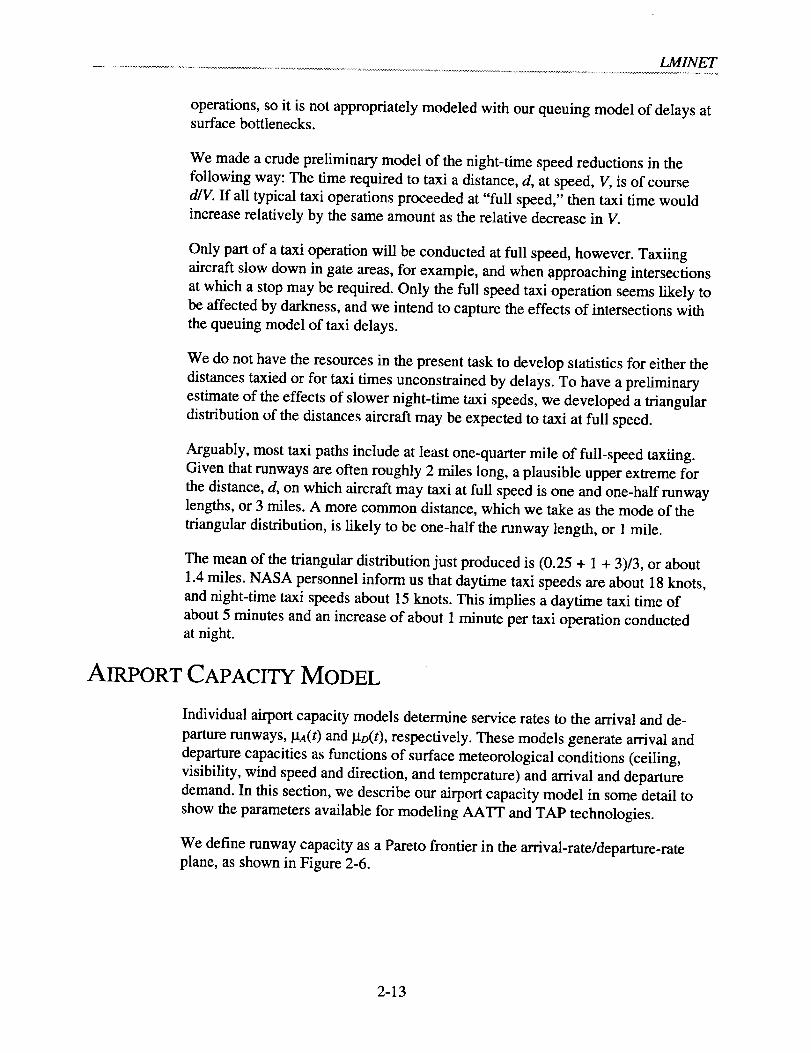
AIRPORT CAPACITY MODEL

Individual airport capacity models determine service rates to the arrival and de-

parture runways, _ta(t) and kto(t), respectively. These models generate arrival and

departure capacities as functions of surface meteorological conditions (ceiling,

visibility, wind speed and direction, and temperature) and arrival and departure

demand. In this section, we describe our airport capacity model in some detail to

show the parameters available for modeling AATT and TAP technologies.

We define runway capacity as a Pareto frontier in the arrival-rate/departure-rate

plane, as shown in Figure 2-6.

2-13

Figure 2-6. Example Runway Capacity

7O

60

o

5O(/)

4o2

_ 30

_ 20

10

0 t I I0 40 50 60 70

F

10 20 30

Arrivals/hou r

All cases of arrival rate/departure rate inside the region bounded by the capacity

curve and the axes are feasible. The capacity curve itself is the set of feasible

points at which not both arrival rate and departure rate can be increased.

We develop capacity from a "controller-based view" of runway operations. That

is, we assume that a human controller manipulates aircraft, introducing time (or,

equivalently, space) increments in traffic streams to meet all applicable rules--

e.g., miles-in-trail requirements, single-occupant rule--with specified levels of

confidence. The desired confidence may differ from rule to rule. For example,

while respecting all rules, controllers may want greater confidence that two air-

craft never attempt to occupy a runway simultaneously than that miles-in-trail

minima are met.

As an example of this approach, consider the arrival-arrival sequence of Figure 2-7,

which shows space-time trajectories of the two arrivals. Zero distance is the begin-

ning of the common approach path, and zero time is the instant at which the lead

aircraft enters the common approach path.

In our model, the controller maneuvers the following aircraft so that it enters the

common approach path a time, _, after the lead aircraft enters it. (The controller

may actually achieve this by bringing the following aircraft onto the common path

when the lead aircraft has advanced a specified distance along the path.) The con-

troller chooses the time interval, kt, through knowledge of typical approach speeds

for the two aircraft and of disturbances affecting their relative positions (winds,

position uncertainties, variations in pilot technique) to ensure that miles-in-trail

2-14

ill I

LMINET

requirements and runway occupancy rules are met with assigned levels of confi-

dence. As we will see in the following subsections, this action of the controller--

together with information on statistics of aircraft operating parameters and the

disturbances to arrival operations, such as winds and position uncertainties--leads

directly to statistics of operations and runway capacity.

Figure 2-7. Flight Trajectories, Gaining Follower

it}

Exl

¢-

0

EE00

t-

O

_D

0C=

121

Runway threshold

1 2 3 4 5 6

I i_ ! Time, minutes

Arrivals Only

We consider first the controller-based paradigm for a runway devoted entirely to

arrivals. Two cases are important: when the following aircraft's approach speed is

greater than that of the lead aircraft ("gaining follower") and when it is less

("lagging follower"). The gaining-follower case also covers the case of equal ap-

proach speeds.

GAINING FOLLOWER

The first of these cases, illustrated by Figure 2-7, occurs when the mean approach

speed of the following aircraft exceeds that of the leader.

In this case, the miles-in-trail constraint applies as the leader crosses the runway

threshold. At that time, the leader's position is D. We will derive a condition on the

controller's interval, gt, to guarantee that the miles-in-trail requirement is met, i.e.,

that at the time the leader crosses the threshold, the follower is at least distance S

away from the threshold, with a specific probability, which we take as 95 percent.

2-15

The position of the lead aircraft is given by

xL = _L +(vL +6VL+ _'_)t [Eq. 2-20]

and the position of the following aircraft by

X F = O°XF+ (V F + b-T'F + b'WF)(t -/1) [Eq. 2-21]

The leader crosses the runway threshold at time tLO, given by

D - O°XLt_.o = [Eq. 2-22]

At time tLo, the follower is at XF(tLO), given by

D- b'XL )x,:(tLo) = _,_ +(vF +,_G +,_v,_) vL +b'VL+b'W,.-p[Eq. 2-23]

We wish to derive a condition on It, to make D-X_tLo) > S, with a probability of

at least 95 percent. To keep the problem tractable, we will assume that all distur-

bances are of first order, and linearize Equation 2-23. When linearized, Equa-tion 2-23 becomes

+DVr(1 b'Vr+b'Wr 8X L 3VL +b'W_ ] _ (b'v_ + 6w_ ) [Ezl. 2-24 ]x,_(t_o) = b'x,_ v_ _, + _. vrV r D V L J /aVr 1"4

In this linear approximation, XF(tLO) is a normal random variable of mean

DV_-- - !aVe and variance

v,

t- tr2r [Eq. 2-25]

The condition that D-XF(tug) > S, with a probability of at least 95 percent, may

then be stated as

+1.6561 <D-S

or

D D-S 1.65o" lla > .... + --

v_ v_ v_[Eq. 2-26]

2-16

LMINET

Inequality in Equation 2-26 gives, in essence, the desired condition. However, Ix is

present on both sides of the inequality. Straightforward manipulations lead to an

explicit condition on It, which, neglecting terms of second order in relative distur-

bances in comparison with one, may be written

l-t > A + x/A2B 2 + C 2 [F_xt. 2-271

where

D D-SA - [Eq. 2-28]

VL V_

2 0"2 tB 2-1.652 trvp + wr

v: lEq. 2-29]

and

:22 22 2 2 2) }1.652 D V: trve+Crwr tr-_+ crv_+cr_ +trxr [Eq. 2-30]C 2 _ .4_ 2

V2 .---T;T-- ,-_ D 2 2 "L v; v;

To determine numerical values of the smallest I.t that meet 2-26, we find the itera-

five scheme

D D-S l'65trl(Pn)_.+I = +

v_ v_ v_

more convenient than using Equation 2-27.

Now let us develop a condition on IXthat will guarantee that the follower does not

cross the runway threshold until the leader has left the runway, with a specified

probability, which we choose to be 98.7 percent. The leader will exit the runway

at time tLo + RAL, and the follower will cross the threshold at time tFO, given by

D- b"Xptro = _-// [Eq. 2-31]

v_ +_ +_v_

Linearizing as previously, we find that in the linear approximation tro--t_ is aD D ---

normal random variable with mean -- + l.t - -- - RAt, where RA L denotes thev_ v_

mean of RAt., and variance

2 DE (0-2 2 2 "_ D 2 (0.2 2 2.

a2 V2_ D 2 V2 ) VL _.D _ .J+crRA L [Eq. 2-32]

2-17

It follows thattheconditionon IXfor the follower not to cross the threshold until

the leader has exited the runway--i.e., that teo-tLx > 0--with a probability of

98.7 percent is

D DIX > _-RA L + 2.215o" 2 [Eq. 2-33]

VL V_

The controller will in effect impose that value of time interval ix that is the small-

est IXsatisfying both Equations 2-26 and 2-32.

Given _t, the time between threshold crossings of successive arrivals is, in our ap-

proximation, a normal random variable of mean

D D+/.t [Eq. 2-34]

Vr VL

and variance

D 2(O.2 2 0.2 '_ D E(O.2 2 2o-3_: _L--D-_-+x.<>"+ _ .)+_/-_-_-__o.,,___+<>-,,L.v/ v; t o v? ;

[Eq. 2-35]

LAGGING FOLLOWER

When the follower's approach speed is slower than the leader's in the controller-

based view, the controller will bring the follower onto the common path after the

leader has advanced a distance S along it, as illustrated in Figure 2-8.

Figure 2-8. Flight Trajectories, Lagging Follower

_6

iE 48

t-

Ot_

82e'-

13

00

..............Threshh ................................

J-_ I 1 I

2 3 4 5 6Time, minutes

ix-,--

2-18

I:1 17

LMINET

Sequences

The positions of the two aircraft as functions of time are again given by Equa-

tions 2-20 and 2-21. The miles-in-trail requirement is now that XL(_)-Xy(p.) > S,

with a probability of at least 95 percent. But

x_ (_) - x_ (#) = _ + (v_ + _ + _w, )_ - _ [Eq. 2-36]

is a normal random variable of mean VLi.t and variance

2 =#2 2 2 2 2{_ 4 ( ff VL + ff WL ) "_- O- XF "I- {_ XL [Eq. 2-37]

It follows that the condition that the miles-in-trail requirement is met, with

95 percent confidence, is

# > _ + 1.65 o-4 [Eq. 2-38]v_ vL

Equation 2-38 may be written as a single condition on _t, using Equation 2-27, by

replacing Equations 2-28, 2-29, and 2-30 with the new definitions

SA_

v_

2 2

B 2 _ 1.65 z o-vL + o-vet , and

2 2

C 2 _ 1.652 o-xz + O-xr

The condition that the single-occupant rule is met with 98.7 percent confidence is

derived exactly as we derived that condition for Vv > VL, i.e., condition Equa-

tion 2-33. In the present case, too, the result is given by Equation 2-33. Also, in

the present case, equations for the mean and standard deviation of interarrival

time, given B, are given by Equations 2-34 and 2-35.

of Alternating Arrivals and Departures

We can readily translate the preceding results for repeated A-D operations, by re-

placing RAt. with RAL + RDn, where the subscript, D, denotes the intervening de-

parture aircraft. This case is illustrated by Figure 2-9.

2-19

Figure 2-9. Flight Trajectories, Mixed Arrival and Departure

E

0.C.[=

£E

oC

5

0

-2

-4

-6 .... I 1 I I 1

0 1 2 3 4 5 6

"Srr rdnutes

It may be desirable to consider the effect of a communications lag, c, on the de-

parture. If so, then RAm is replaced by RAm + c + RDo.

Statistics of Multiple Operations

At this point, we have expressions for the means and variances of normal random

variables representing interarrival times for two cases: when the runway is used

for arrivals only and when it is used for alternating arrivals and departures. Now

we wish to use these to generate statistics of multiple arrivals, or multiple arrivals

and departures, to capacity curves for single runways.

First, we consider the statistics of sequences of arrivals only. Statistics of the

overall interarrival time will be determined by the mix of aircraft using the run-

way, with their individual values of the aircraft parameters of Table 2-2. Suppose

n aircraft types use the runway, and let the fraction of the aircraft of type i in the

mix be pi. Then the results of the preceding sections give interarrival time for each

leader-follower pair as a normal random variable. Let tAAUdenote the random

variable that is the interarrival time for aircraft of type i following an aircraft of

typej. As we have seen, in our model tAAUis a normal random variable; let its

mean and standard deviation be gv and _ij, respectively.

2-20

HI[ _r-

LMINET

Table 2-2. Runway Capacity Parameters

Symbol, DefinitionXC

5cD

DoPiRA_

5RAiROi_RDi

D

S_j

IMC

Reciprocal of mean input-stream delay

Mean communication time delay

Standard deviation of communication time delay

Length of common approach pathDistance-to-turn on departure

Fraction of operating aircraft that are type i

Mean arrival runway occupancy time of ith aircraft typeStandard deviation of arrival runway occupancy time of ith aircraft type

Mean departure runway occupancy time of ith aircraft typeStandard deviation of departure runway occupancy time of ith aircraft type

Miles-in-trail separation minimum, aircraft of type/behind aircraft of type jDeparture miles-in-trail separation minimum, aircraft of type i behind aircraftof type j

Binary variable; 1 means instrument meteorological conditions prevailApproach speed of aircraft type iStandard deviation in approach speed of aircraft type li

Wind variation experienced by aircraft of type i

Standard deviation of controller's information on position of aircraft i

Now, to determine the distribution of the overall interarrival time, tAA, we consider

a classical "urn" problem: we have a population of interarrival times, from which

we draw one member, and we wish to know the distribution function of the result.

The probability of drawing tAAU is PiPi, and the distribution function of the result is

the weighted sum of the distribution functions for the individual taai./. That is, the

distribution function for the overall interarrival time taA(1) is

tax(1)~_,___PiPjN(t;lao,cro)

i j

['Eq. 2-39]

where N(t; It, c) denotes the normal probability distribution function. Obviously,

the distribution of interarrival times is not necessarily normal. An example of an

interarrival time distribution of the type Equation 2-39 is shown in Figure 2-10.

2-21

0.02

0.018

0.016

0.014

0.012

0.01

0.008

0.006

0.004

0.002

0

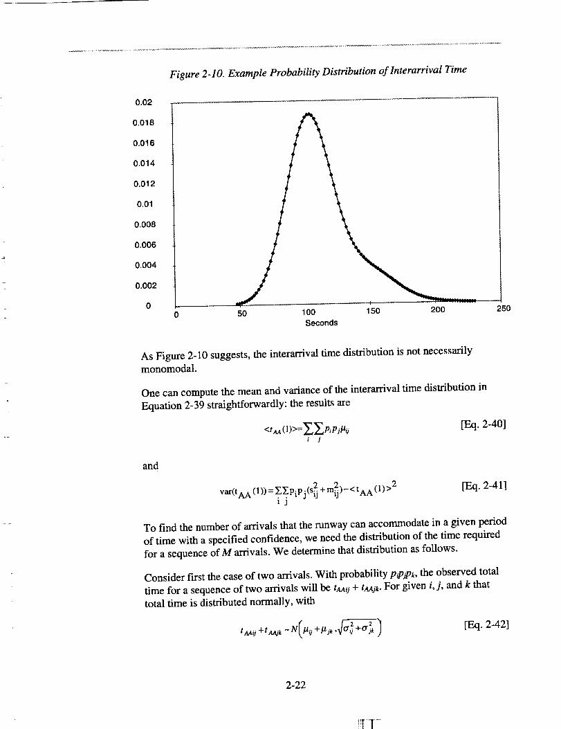
Figure 2-10. Example Probability Distribution of lnterarrival Time

0 50 100 150 200 250

Seconds

As Figure 2-10 suggests, the interarrival time distribution is not necessarilymonomodal.

One can compute the mean and variance of the interardval time distribution in

Equation 2-39 straightforwardly: the results are

<t an (1)>= EEpi pflaij [Eq. 2-40]i j

and

var(tAA (1))-- ._PiPj(S _ + m2)-< tAA (I)>2IJ

[Eq. 2-41]

To find the number of arrivals that the runway can accommodate in a given period

of time with a specified confidence, we need the distribution of the time required

for a sequence of M arrivals. We determine that distribution as follows.

Consider first the case of two arrivals. With probability p_o_ok, the observed total

time for a sequence of two arrivals will be tAAU+ tAAjk. For given i, j, and k that

total time is distributed normally, with

taail +t'_Jk- N( llil+lljk '_1 [F.xt. 2-42]

2-22

LMINET

Thus, the time taa(2) for a sequence of two arrivals will have the distribution

2 2[Eq. 2-43]

where the sums range over the number of aircraft in the mix.

Continuing in this way to reckon the distributions of the time required for 3, 4, ...,

M arrivals, we conclude that taa(M) has the distribution

£_._...£pipj...pypzN(t_ _+t2j _ 2 2 2+ojk+...+o;z). [Eq. 2-441

In Equation 2-25, the sums range over the set of aircraft using the runway. There

are M + 1 summations, and M + 1 terms in Pi Pj." Py Pz" There are M terms in2 2 2

both the sums/.tii + Pik +...+/zyz and cr0 + trjk +...+cry z .

Evaluating the expected value <taa(M)> is straightforward. We find

<taA(M)>=ZZ--.'___PiPj..-pyPz(IIi j +/tjk +"+/_ya) ' [Eq. 2-451

which leads directly to

<t AA( M)>=--M££piPj_'j , [F-xl. 2-46]

since the p; sum to one.

Evaluating the variance of tAa(M) is more involved. After considerable manipula-tion, we find

var(tAA (M))=M£Zpipj(a 2 +_)+2(M-1)£ZZpipjpk/4..ill.tjk -(3M-2)(ZZpiPjli4. j )2 .[Eq. 2-47]

In Equation 2-47, the sums again range over the set of aircraft types that use the

runway.

Evaluating the number of arrivals that a runway can accommodate in 1 hour, with

assigned confidence, is conceptually straightforward: one finds the largest M for

which the cumulative distribution corresponding to the probability distribution

Equation 2-44, evaluated at 3,600 seconds, is not less than the desired confidence.

It is tempting to approximate the distribution in Equation 2-44 with a normal dis-

tribution for this purpose, since direct evaluation of the cumulative distribution

function corresponding to Equation 2-44 involves lengthy sums when M takes

values near typical hourly arrival numbers, which are around 30.

If the individual interarrival times in a sequence of arrivals were statistically inde-

pendent, an appeal to the central limit theorem would justify that approximation.

2-23

Of course,theyarenot independent,becausethefollower in agivenpair is theleaderfor thenextpair of thesequence.

Nevertheless,numericalexperimentssuggestthatmembersof thefamily of distri-butionsinEquation2-44arewell approximatedby normaldistributions,evenforfairly smallM, even when the distribution of a single interarrival time departs

considerably from a normal distribution. Figures 2-11 and 2-12 illustrate this, with

the distribution functions of the time for two and for four arrivals, respectively.

The single-arrival distribution is the same as that of Figure 2-10.

In view of results like those of Figures 2-11 and 2-12, we approximate the distri-

bution of the time required for M arrivals as a normal distribution whose parame-

ters are the mean and variance given by Equations 2-46 and 2-47, respectively.

Then the largest number of arrivals that the runway can accommodate in 1 hour,

with 95 percent confidence, is the largest value of M for which

< taa (M) > +l.65x/var(taa (M)) < 3,600, [E,q. 2-48]

where tAA(M) and var[taa(M)] are evaluated by Equations 2-46 and 2-47, respec-

tively. For the case illustrated by Figures 2-10, 2-11, and 2-12, this leads to a ca-

pacity of 30 arrivals per hour.

An alternative definition of runway capacity is the largest number of arrivals for

which the expected total time is not longer than 3,600 seconds. With this defini-

tion, the capacity of the runway for the case illustrated in the figures is 32 arrivals

per hour.

2-24

i_i1

LMINET

Figure 2-11. Distribution Function of the Time for Two Arrivals

1 .20E-02

1 .00E-02

8.00E -03

6.00E -03

4.00E-03

2.00E-03

0.00E+00 5'0 100 150 200 250 300

Seconds

Figure 2-12. Distribution of the Time for Four A rrivals

9.00E-03

8.00E-03

7.00E-0G

6.00E-03

5.00E-03

4.OOE-03

3.OOE-03

2.00E-03

1.00E-03

0.00E+00100

SS-:--S:??S-S?S-_--Z--7

200 300 400 500 600 700 8O0

2-25

Input-Stream Effects

So far, we have developed our model as though the controller could always im-

pose the desired time separation, It, whatever the nature of the incoming stream of

aircraft. This may not in fact always be the case, and we extend our model to

cover input-stream effects in this way:

We suppose that the controller, wishing to impose separation It, is actually able to

impose the separation It + v, where v is a random variable, independent of all oth-

ers in the analysis, characterizing input-stream effects. We take v to have the ex-

ponential distribution with parameter _,, i.e.,

V - _e -_'v . [Eq. 2-49]

With the addition of the random variable, v, the distribution of interarrival times

for a fixed leader-follower pair is no longer a normal random variable, but the

convolution of a normal random variable and an exponential random variable.

Specifically, the distribution is

(t-r-#) 2®- ;tr

H(t;/_,tr,A)-=---_ ----- fe 2a2 dr.

42herdo

[Eq. 2-5O]

This distribution function may be evaluated conveniently using

_2a2

• _ -;t(t-/_)+_ 2n(t,l_,tr,_.)-Ae [1- C(/l,t-,_r ,(r)]. [Eq. 2-51]

where C(x,/_,a) denotes the cumulative normal distribution for mean It and stan-

dard deviation t_, evaluated at x.

Figure 2-13 shows an example of this class of distribution, together with the nor-

mal distribution that would have been seen absent input-stream effects• The ex-

ample of Figure 2-13 is somewhat extreme, for the sake of illustration. Typically,

input-stream effects would introduce a mean error of 10 seconds or less.

With our model of input-stream effects, the distribution of interarrival times

changes from Equation 2-39 to

tag (1) ~ _ y_.pipjH(t;_tij,oij,k )i j

[Fx t. 2-52]

2-26

l_ 1

LMINET

Figure 2-13. Example Interarrival Distribution with Input-Stream Effects

o 012

O.DI

0008

O.OOS

0 _1_4

0.O02

0

I Ith "l,pulllrenm *tfe©t*" "4B--N orm :* [

]•--4_-.. W

J

,¢0nd

_S0 200 250 300

IA T_JigandI

and the distribution function of taa(M) changes from Equation 2-44 to

where

2-53]

g % (t-*-/_) 2

;t /H(t;It,a,_,,K)= r --- It - e dr

42tea(K-I)! d0

[Eq. 2-54]

It is not difficult to show that the mean and variance of tAa(M) may be obtained

from the values in Equations 2-46 and 2-47, simply by adding MFL to <tAA(M)>

and M/(_, 2) to var(tAa(M)). With these results, and the assumption that the distri-

bution of taa(M) may be adequately approximated by a normal distribution for suf-

ficiently large M, we may compute runway capacities with our model of input-

stream effects. For example, taking the value l/_, = 6.3 seconds, which certain

data for operations at DFW suggest, reduces the 95-percent-confidence capacity to

28 arrivals/hour, and the "expected-total-arrival-time" capacity to 30.

Completing the Pareto Frontier of Runway Capacity

At this point, we have developed our model for one point on the Pareto frontier

that describes runway capacity, the point for all arrivals and no departures. We

give this fairly complete discussion of that point because it is often a very impor-

tant one and to illustrate our modeling work.

We completed our runway capacity models by systematically continuing the ap-

proach described previously, to cover three other cases: when the runway is de-

voted wholly to departures, when the runway operates with alternating departures

2-27

andarrivals,andwhentherunwayoperateswith as many departures as possible,

while continuing to accommodate the same number of arrivals as in the arrivals-

only case. We thus characterize the Pareto frontier by four points.

When these steps are completed, several parameters characteristic of a specific

airport are found to affect runway capacity. The complete list of capacity parame-

ters is shown in Table 2-2.

In addition to the runway capacity parameters, LMINET's airport capacity models

respond to information on the configurations in which the airport is usually operated.

This information includes the specific runways that make up the configuration, with

their individual minimum visibility restrictions. Our airport capacity models system-

atically select the configuration most capable of meeting demand, in view of mete-

orological conditions. The airport models report the feasible arrival-rate/departure-

rate combination that best meets demand as the airport's instantaneous capacity.

MODELS OF TRACON AND ARTCC SECTORS

Recent work done for NASA at the Institute has produced new models of both

ARTCC and TRACON sectors as multiserver queues, specifically as M/EdNIN+q

queues. That is, as queues with Poisson arrivals, service times with the Erlang

distribution with parameter k, and N servers; not more than q clients will wait for

service, so the maximum number in the system is N + q.

The models were developed with input from FAA people, including controllers at

the Denver ARTCC and the Denver TRACON as well as experienced supervisory

controllers working at the FAA's National Command Center in Herndon, VA.

The development and calibration of the queuing models of sectors is described in

[1]. The following section gives some details of the model and of the numerical

treatment that we made for operating LMINET.

M/E3/N/N+Q Sector Model

In our queuing model for the ARTCC and TRACON sectors of the NAS, thetimes between aircraft arrivals to each sector are assumed to have the Poisson

distribution, and the time that an aircraft stays in a sector is assumed to be a ran-

dom variable distributed according to Erlang-3 distribution. A sector can simulta-

neously handle no more than N aircraft at a time, where the capacity N is

determined by the sector's characteristics and the weather. We also assume that, at

most, q aircraft will "wait"--i.e., be delayed by speed changes or vectoring--to be

served in a sector.

The arrival demand for a sector is determined by the network flight schedule. The

choice of the Erlang-3 distribution for the times-in-sector was made in view of

ETMS data and is explained in [1]. We chose 18 as the maximum number of

2-28

LMINET

aircraft that a sector's controllers can handle at one time, to be consistent with

[13]. We base our choice of the maximum number of "wait" aircraft on interviews

with controllers at the Denver ARTCC.

Solving the model poses a significant challenge. There is no closed form solution,

not even for the steady state, for the MIEklNIN+q queue. We determine the prob-

abilities of each state of the system numerically.

That is itself a respectable challenge because the number of states is large. For a

MIE31NIN+3 system, there are 1,950 states. [6] The number of states increases

rapidly with N. For example, if q = 3, the number of states is 27,000 if N is 50, the

number of states is 192,000 ifN is 100, and the number of states is 620,000 ifN is

150. Thus, determining the state probabilities directly from the evolution equa-

tions means solving a very large system of ordinary differential equations.

The systems' plant matrices are sparse, and the systems seem reasonably well-

conditioned, so that brute-force numerical methods may succeed for some cases.

We have, in fact, generated numerical solutions of the full equations for N=18 and

q = 3 in this way, to have means of checking the results of approximate solution

methods. This approach takes too much time, however, to be at all appealing for

routine use. Fast-executing approximate solutions are greatly to be desired. The

trick lies in reducing the number of states.

Our key idea for improving the computer execution involves a new concept called

mega state. The Erlang-3 distribution is mathematically equivalent to the distribu-

tion that results from service by three servers in tandem, each of which has the

same Poisson distribution of service times. Thus, the state of an MIE3/N/N+q sys-

tem is determined by four numbers i,j, k, and q, where i denotes the number of

aircraft that have not completed one service of the three required, j denotes the

number that have completed one but not two services, k is the number that have

completed two but not three, and q is the number of aircraft waiting.

The mega state, m, is defined as m = i + j + k. If the sector capacity is N, then

me [0,N]. After checking the state transition matrix, we realized that a state inter-

acts only with states of neighboring mega states. This further implies that for

mega states ml, m2, ml< m2, if Pr(ml)=0, then Pr(m2)--O, which can be proved bymathematical induction.

In practice, we can maintain a dynamic upper bound of the mega state such that

the probability of any mega state less than this upper bound is nonzero and the

probability of any mega state equal or larger than this upper bound is negligibly

small. Therefore, we do not need to solve all the state transition equations; we

need to solve only the ones whose mega state is equal to or less than the upper

bound. This technique alone reduces more than 90 percent of computer execution

time. Since the upper bound is dynamic, there is virtually no loss of accuracy of

solution, which we have verified by comparison with exact solutions.

2-29

For solvingthosestateevolutionequationsthatmustbesolved,wehavetriedforwardEuler, second-andfourth-orderRunge-Kuttaintegrationschemes.Of thethree,thesecond-orderRunge-Kuttagivesusthebestspeed,contraryto the con-ventionalwisdomthatthefourth-orderRunge-Kuttawould.Thehighertheorderin theRunge-Kuttaintegrationscheme,themoreaccuracywemayget;hence,wemayafford largerintegrationstepsto speedup theprocess.However,dueto thelargenumberof differentialequationswith which wehaveto deal,stiffnessislikely to preventourusinglargesteps.Wefinally settledon the second-orderRunge-Kuttaschemewith adaptivestep.

Theadaptivestepcontrolworksasfollows. In movingthetimeby onestep,wealsomovethetimeby twohalf steps.Wethencomparetheirresults.If their dif-ferenceis smallerthanaspecifiednumber,wewill enlargethestepin thenextiteration;if their differenceis largerthanaspecifiednumber,wewill reducethestepandgobackto redothis integrationstep.Their differencesarealsousedtogetbetterprecision.In workingout severalcases,we find thatwegainasmallfractionof thetotal timeby usinga second-orderRunge-Kuttaschemewithadaptivestepsize.

Anotherimportantmethodfor keepingthequeuingcalculationstractableis to in-troducesubsectors.This is particularlyhelpful for therectangular-areasectorsofLMINET, whichcanhavelargepeakdemands.

In operatingtheNAS,theFAA subdividesbusysectors,geographicallyand/orbyaltitude.We modelthisby oursubdividingbusysectorsinto setsof independentsectors,eachof whichhastheN of a single sector. We have been careful not to

carry this process beyond the point at which the subdivisions are at least arguably

feasible for actual operations.

LMINET's rectangular en route sectors are roughly 120 miles on a side. They

represent airspace above Flight Level 230. With present altitude-direction

conventions, this affords about 14 levels at which modem turbojet transports may

cruise: eastbound traffic at flight levels 230, 250, 270, 290, 330, 370, and 410;

westbound traffic at flight levels 240, 260, 280, 310, 350, 390, and 430.

Thus, division into two subsectors can be accomplished feasibly, either by altitude

or geographic sectioning: two geographic subsectors would be 60 x 120 nautical

miles, and two altitude subsectors would each have 7 available flight levels.

Subsectoring with two geographic subsectors and two altitude subsectors is also

feasible, so divisions with four subsectors are feasible.

Subsectoring into three geographic regions could certainly be accomplished feasi-

bly, giving sectors 40 x 120 miles. Division of a rectangular sector into three sub-

sectors by altitude division probably is feasible, as well: each subsector would

2-30

I'! 'I ',

LM1NET

have at least two altitudes. But the resulting combination, giving nine subsectors,

may be about as far as one should go.

Internally, LMINET assumes that aircraft arriving at a subsectored sector are

roughly evenly divided among the subsectors. Queue statistics are generated for

just one of these, so, to get overall delay statistics, one scales up the single-sector

result by the number of subsectors. The advantage for the queuing calculations is

that we never consider a sector capacity N larger than the value, typically 18, that

is characteristic of a single controller team.

With megastates and subsectoring, and compiling the C code in which LMINET is

written to optimize execution speed, we can generate statistics for one 20-hour

"day" of CONUS operations in roughly 15 minutes on LMI's HP D370 withRISC 2.0.

TRACON Models

Each airport's TRACON is modeled with two arrival sectors and one departure

sector. All the sectors are modeled as M/Ek/N/N+q queues.

LMINET allocates arrivals to an airport so that each arrival TRACON sector sees

roughly half of the arrivals in each epoch of operation. For the work reported here,

an epoch is 1 hour long.

En Route Sector Models

Like the TRACON sectors, en route sectors are modeled as M/Ek/NIN+q queues.

Automatic Traffic Flow Controller

This element of LMINET models the FAA's practice of delaying scheduled air-

craft departures to congested airports. The function of this module can be

summarized as limiting the arrivals to each airport by the airport's arrival capacity

for each time epoch of the day so that large arrival queues never form.

To perform this function, we construct a planning window, composed of the rest

of day, to facilitate the planning of ground hold decisions. At each epoch of the

day, the module checks each airport's arrivals for the rest of the day. If the sched-

uled arrivals exceed the arrival capacity, the module will move some arrivals to

the next epoch so that arrival demand meets capacity.

This process continues successively to the end of the day for each airport. Once

this is done, the departure schedule is permanently changed, based on the delays

calculated during the process. The arrival queue and departure queue at the end of

the last epoch are counted as additional demands to arrival and departure at the

2-31

currentepochin theplanningwindow,andthequeuefor planesfrom thelastepochiscountedasdemandto botharrivalanddepartureat thecurrentepoch.

Evenwith thetraffic flow controller,wecannottotallyeliminatethearrivalqueuesdueto thefact that (1)wecannotdelayanaircraftthatis alreadyin depar-ture,(2)wewill not delaythearrivalsfrom theout-of-networkairport, (3)airportcapacitiesaredynamicanddependuponbotharrivalsanddepartures,whichmeansthatarrivalsmayexceedthearrival capacityevenif arrivalsequalcapacityin theplanningdueto thelargedeparturedemand,and(4) delaysarealwayspos-siblein a queuingsystem.

We implementtheautomaticflow controllerin accordancewith thefollowingguidelines:

Only departuresto the congested airport will be delayed. The amount of

delay is equally distributed among all the flights eligible to be delayed.

We will not delay the departures from the congested airport to reduce

congestion.

• Only the flights in the network airports may be delayed. The departures

from airports outside the 64-airport network will not be delayed.

We assume each airport is independent in its traffic flow control planning,

and the decision to delay flights to the congested airport is solely based on

the current schedule, current delays and queues, and forecasted airport ca-

pacities. Since the air traffic flow control planning is done at each epoch

for the rest of the day for each airport, the network effect of the traffic flow

control is done through the modified schedule for the rest of the day.

TRACON congestion is not a decision criterion.

• Local weather information, for the rest of the day, is assumed to be known

to the air traffic controller at any time of the day.

• A flight can be delayed repeatedly as long as it has not yet departed.

The typical cause of airport and TRACON congestion is inclement weather,

which will reduce both capacities. However, as we found out, we do not need to

specifically count TRACON congestion as decision criterion because once the

arrivals and departures are curtailed, the demand to the associated TRACONs willalso be reduced.

2-32

1'7I

Chapter 3

Adjusting LMINET to Model the NAS

Users may adjust several LMINET inputs: demand prof'fles, airport capacity mod-

els, sector capacity models, surface weather and weather aloft, routes between air-

ports, and so on. This chapter explains our choices for the baselines.

DEMAND INPUTS

In general, the demand input to an NAS model must provide all requests for serv-

ice, at any time and anywhere in the NAS. Since other inputs to LMINET provide

the four-dimensional (4-D), or space and time, flight trajectories between every

airport pair, and since LMINET has models that handle the queues and delays, the

principal demand input to LMINET is the flight departure schedule, so_, where i, j

I = {0,1 ..... 64} and k e K={0,1 .... ,20}. Here i andj are the indices of the air-

ports in the LMINET, where 0 represents an out-of-network airport, and k is the

time index, where 0 represents the beginning of the day (0600 EDT). For this

study, we operated LMINET in 1-hour epochs, so that the 21 epochs cover the pe-

riod from 0600 EDT to 2300 Pacific time.

The remaining demand inputs to LMINET are a_t, arrivals to airport i at epoch k

from outside the network, and b_k, extra-network arrivals to sector i at epoch k. For

this report, we input extra-network arrivals to an arrival TRACON at each airport

and to the airport's arrival queue.

Demand in 1996

We considered both scheduled air transport service and itinerant GA traffic. We

based demand for scheduled air transport service on the schedule published by theOAG. We constructed the time variation in GA demands from data recorded in

the ETMS. Since the OAG schedule is the planned rather than the observed air

traffic schedule, and only the GA filing IFR will be recorded in ETMS, both the

OAG and GA schedules are scaled to conform with the corresponding data givenin the FAA's TAF.

April 8, June 12, and November 22, 1996, are the days for which we run our

model. We chose these in view of the variation in weather throughout a year. The

demand schedule we used for each specific day is based on the OAG for that day.

3-1

Demand in 2007

The future air traffic demand, expressed in terms of the schedule, SUk,must be

constructed. Our construction method is based on the current schedule, the TAF,

and a traffic distribution model. Since the TAF forecasts airport-specific growth

rates, one cannot generate future traffic demands by simply multiplying each air-

port's departure demands by its individual growth rate: to do that would not givethe desired new arrival rates at the other airports.

In fact, generating demand schedules for the entire network corresponding to indi-

vidual overall growth rates at its airports is a challenging task. The following sub-

sections review our methods for determining the individual growth rates and

developing future demands.

AIRPORT OPERATIONS GROWTH RATE

The TAF is our data source for the growth rate of airport operations. We used the

total of air carder, air taxi, and itinerant GA in the TAF as the airport operations

measure. Air carder and air taxi are the operations of scheduled air transport

service corresponding to the OAG; air taxi is for aircraft with less than 60 seats,

which is typical of commuter operations. For the most recent TAF, released in

February 1998, the data from 1976 to 1996 are the annual totals reported by the

airport control tower, while the data from 1997 through 2010 are the FAA's pre-

dicted values. From these predictions, we can derive the operations growth rate

from the baseline year 1996 to the target year 2007. Since the forecasts stop at

year 2010 in the TAF, we used the last year's growth rate from 2009 to 2010 re-

ported under each category and by each airport and then compounded it to get the

forecast beyond 2010

The forecasted operation figures for major airports in the TAF are derived by FAA

in the following ways: (1) forecasting the enplanements based on the socioeco-

nomic models; (2) forecasting the load factors to and from each airport based on

the demand, fare yield, and airlines cost; (3) forecasting the average number of

seats per aircraft for arrivals and departures at the airport; and (4) dividing the

forecasted enplanement by the forecasted load factor and by the forecasted aver-

age number of seats per aircraft.

Table 3-1 shows the FAA's values for operations and enplanements at the

LMINET airports for 1996, 2007, and 2017. Tables 3-2 and 3-3 compare

LMINET to the network for operations and enplanements, respectively. Figures

3-1 and 3-2 graphically depict the LMINET airport annual operations and en-

planements for 1996 through 2017.

3-2


Table 3-1. Annual Operations (thousands) and Enplanements

(millions) at LMINET Airports

Airport

BOS

BDL

HPN

ISP

TEB

LGA

JFK

EWR

PHL

BWl

DCA

lAD

GSO

RDU

CLT

ATL

MCO

PBI

FLL

MIA

TPA

MSY

IMEM

BNA

SDF

CVG

DAY

CMH

IND

CLE

DTW

P_

SYR

MKE

ORD

MDW

STL

IAH

HOU

AUS

1996

462

151

153

109

189

342

360

443

401

26O

305

323

138

217

454

770

337

182

234

540

269

162

358

222

168

392

143

185

230

287

53O

438

122

187

906

251

511

391

252

203

Operations

2017 19962OO7

509

181

160

117

189

381

397

561

509

338

318

397

170

256

563

916

5O2

196

304

694

331

190

467

26O

215

613

160

238

3O5

373

708

536

148

239

1039

297

637

566

287

245

543

214

159

122

189

413

432

661

584

411

33O

463

187

285

656

1050

665

207

365

850

396

215

581

285

243

818

176

268

375

450

873

628

170

276

1182

335

752

728

319

299

12.3

2.7

0.5

0.6

0.0

10.3

15.0

14,2

9.1

6.6

7.2

6,0

1.4

3.1

10.7

30.7

11.8

2.8

5.2

16,1

6.2

4.2

4.6

3.4

1.8

8.8

1.0

3,1

3.5

5.4

15.0

10.1

1.0

2.7

32.2

4.5

13.5

11.9

4.0

2.8

Enplanements

2007

16.0

4.1

0.9

0.9

0.0

13.8

20.7

20.7

14.8

10.3

8.6

9.7

2.5

4,8

15.6

41.4

22.6

3.9

9.4

27.4

9.2

5.9

6.2

5,4

2.9

16.9

1.0

5.3

5.8

8,6

24.7

14.4

1.3

4.3

43.2

6.4

20,5

20.0

5,3

4.6

2017

18.9

5.9

1,3

1,3

0.0

17.0

26.0

26.7

19.7

13.8

10.1

13,3

3.5

6.9

20.1

51.3

32.8

4.9

13.2

38.3

12.0

7.5

7.7

7.3

3.9

24.6

1,1

7,3

7.9

11.5

33.8

18.5

1.5

6.1

53.9

8.4

27.0

27.5

6,6

6.2

3-3

Table 3-1. Annual Operations (thousands) and Enplanements

(millions)at LMINET Airports (Continued)

Operations Enplanements

Airport 1996 2007 2017 1996 2007 2017

SAT

DAL

DFW

MSP

MCI

DEN

ABQ

ELP

PHX

SLC

LAS

SAN

SNA

LGB

LAX

BUR

i ONT

RNO

SMF

OAK

SFO

SJC

PDX

SEA

238

219

869

478

195

453

173

122

531

369

445

238

369

263

761

180

149

144

145

4OO

426

210

290

397

293

264

1234

615

244

553

217

125

698

491

637

309

483

312

947

222

177

189

201

494

562

258

384

5O3

359

305

1571

742

285

644

258

128

854

6O4

815

376

588

356

1120

262

203

216

241

581

687

302

471

601

3.3

3.5

27.4

13,4

5,0

15.2

3.2

1.8

14.6

9.8

14.3

6.8

3.6

0.2

28.2

2,5

3.2

3.0

3.5

4.8

18.3

4.8

6.1

11,7

5.5

5.2

43,7

20.8

7,1

20.6

5.1

2.8

24.2

15.5

26.1

10,4

6.4

0.4

41.9

4.3

4.6

5.4

5.7

7,8

29.4

8.0

10.2

17.5

7.6

7.0

59.0

27.8

9.0

25.5

6.9

3.8

33.3

20.8

37.3

13.7

9.0

0.6

55.0

6.1

6.0

7.6

7.8

10.7

38.3

11.0

14.1

22.8

Table 3-2. LMINET Airports Versus the Network (operations)

Operations (millions)

Growth rate Growth rateLocation Count 1996 2000 2010 1996-2000 2000-2010

Large hubs

Medium hubs

Smallhubs

Nonhubtowem

29

42

67

305

LMINET airports

13.6

9.2

8.2

30.9

14.9

9.9

6.6

31.8

18.3

11.6

9.3

33.5

2.37

2.04

1.24

0.70

2.04

133

0.74

0.54

Total 443 61.9 65.3 72.7 1.35 1.08

64 20.7 22.6 27.3 2.20 1.91

3-4


Table 3-3. LMINET Airports Versus the Network (enplanements)

Enplanements(millions)

Gmwth GmwthLoc_ion Count 2010 rate rate

1996-2000 2000-2010

Large hubsa

Medium hubsb

Small hubsc

Non hub towers

29

42

67

273

684.3

237.9

67.5

22.2

1996 20O0

412.6 490.1

135.7 163.6

41.6 48.8

15.5 17.6

605.5 720.2

514.0 613.0

85.0 85.1

4.40

4.79

4.08

3.18

3.39

3.81

3.30

2.38

Total 411 1,012.0 4.43 3.46

LMINET airports 64 863.0 4.50 3.50

Share of LMINET airports 85.3

Source: Department of Transportation, Termina/ Area Forecasts, Fiscal Years 1997-2010, ReportNo. FAA-APO-97-7, Federal Aviation Administration, Office of Aviation Policy and Plans, Statistics andForecast Branch, Washington, DC, October 1997.

a> 1% of total enplanement

b > 0.25% of total enplanement

c > 0.05% of total enplanement

Figure 3-1. Total LMINET Airport Annual Operations (millions)

35.00

30.00

25.00

20.0O m GA /

15.oo l [] Commerc al i'

10.00

5.00

0.00 ,

3-5

Figure 3-2. Total LMINET Airport Annual EnpIanements (millions)

m Enplanement

FRATAR ALGORITHM

This algorithm is the most widely used method of generating trip distributions

based on the terminal area forecast. It has been used by both DOT and FAA in

their transportation planning models, such as the National Air Space Performance

Analysis Capability (NASPAC), an event simulation model of NAS. The traffic,

tij, from airport i to airport j, total departures, d/, from airport i, and total arrivals,

aj, to airport j are related to the schedule, sijk, as follows:

t# = ,Y-.ks#k,

di = _,j t O,

aj = _,i to.

If the schedule is balanced, or the network does not have any sinks, then di = ai, V

ieI.

Let Di, i _ I be the total number of departures in the target year taken from the

forecast. The Fratar method is an iterative algorithm that takes the following

steps:

Step 0: Assign t0, di, aj, Vi, j e I, based on the current year schedule.

3-6

ii! it_


Step 1:

Dgi =- ',Vi_l,

di

Step 2:

TO =tij'gi'gj" " _ - • ,Vi,j

rt J

Step 3:

If Z_j=Di,Vi_I, then go to Step 4;

else

tij= To, Vi, j _ I,

update di, aj, Vi, j _ I accordingly, go to Step 1.

Step 4: Compute the traffic growth factor r U, Vi, j _ L by dividing the traffic TU in

the target year by the one in the current year; compute the schedule Sijk in the tar-

get year by multiplying the schedule in the current year by the traffic growth factor

r 0. Stop.

The schedule in the target year made by the Fratar algorithm has some interesting

properties. First, the schedule will always meet the terminal departure totals pre-

dicted in the TAF. Second, r U= rji, which means the traffic growth is undirec-

tional. Third, the growth factor is u mform across the entire day, which is a desired

property if we assume that the underlying time-of-day travel demand pattern in the

future is unchanged and the schedules are designed to best serve the demand

across the day. Unless there is any drastic change in air transportation technology

that will substantially reduce travel time, it is reasonable to assume that the same

time-of-day demand pattern will remain the same in the future. Another assump-

tion hinges on the rational behavior and maturity of the air transport industry. The

airline industry appears to have reached its maturity two decades after its deregu-

lation. For the past few years, the industry has enjoyed record profits, stable net-

work configuration, steady capacity growth, and rational route development in

contrast to the record loss, brutal market share competition, explosive capacity

growth, countless startups, and massive industry consolidation typical in the years

just after deregulation.

3-7

Thefact thatthegrowthfactoris uniform acrossthedayimpliesanotherpropertyof theschedulein thetargetyear:theairport traffic is dynamicallybalanced,andthebankoperationsin hubairportsarepreserved.Let dik, ajk, Vi_ L Vk _ K, be

the total departures and arrivals in time k.

elk -" _j Sijk,

aik = _j sjik.

An airport i is said to be dynamically balanced if dig = aik, Vk _ K, which means

there are no idle aircraft sitting on the ground. In reality, a flight has to spend

some time in the terminal before taking off, but we will keep this simple defini-

tion, and real operations can be modeled by shifting the time index. Let Di_, Aik,

Vie L Vk e K, be the total departures and arrivals at airport i at time k in the tar-

get year. By the Fratar algorithm,

Dik = _j Siyk = Y_yr_isiyk= Gi _,y uy sijk,

Aik = _,j Sjik : Zj rji Sjik = Zj rij Sjik = Gi _j uij sijk,

where

Gi uj = rU, Vi, j _ I,

_juj= 1.

Now one can see that the right hand sides of Dik and Aik resemble the expectations

of the product of two discrete random variables. If two random variables are inde-

pendent, then the expectation of their product is equal the product of their expec-

tations. If we assume that the traffic growth rate is independent of the current

schedule (which is a reasonable assumption), then

Dik = Gi (_j uj)( _j Sijk,) = Gidi_,

similarly,

Aik =- Giaik.

Since dlk = aik, Vi _ L Vk _ K, then Dik = Aik. And, interestingly, Gi must be the

growth factor implied by TAF in order to satisfy the binding terminal total depar-ture constraint.

CAPACITY MODELS

This section explains how we adjusted our airport capacity models to make a

baseline case for 2007. We treat the airside and surface-delay models separately.

3-8

!!!ili


Airport Airside Capacity Models

We derived the 64 airport capacity models in two steps. The initial development

was done for NASA as Task 97-10, "AATT Benefits Prioritization," under con-

tract NAS2-14361. This development used two sources. For the 10 airports treated

in the TAP studies LMI performed for NASA, ! we developed models from dis-

cussions with controllers at the individual airports. For the remaining airports, we

developed models by reviewing airport diagrams in the several volumes of U. S.

Terminal Procedures, published by the Department of Commerce. (These flight

information publications are commonly called "approach plates.")

We validated the models in two ways. First, we operated LMINET with universal

good weather inputs and observed that the outputs indicated minimal, but not

zero, delays. We also observed that the total number of aircraft required in the air-

ports' initial ready-to-depart reservoirs is roughly 80 percent of the total number

of aircraft in the commercial fleet for 1994, as reported in the FAA Statistical

Handbook for 1994. This is consistent with the fact that the LMINET airports ac-

count for roughly 80 percent of CONUS operations.

The second validation was by discussing the results with controllers at the FAA's

Command Center. The controllers with whom we spoke agreed with the LMINET

outputs in some cases and disagreed in others. When there was disagreement, we

modified our airport capacity models in accordance with the controllers' sugges-tions.

For the present study, we extended the models developed under Task 97-10 to in-

clude input-stream effects, as described previously. Our baseline capacity models

infer the mean time impact of input-stream effects (i.e., the value of 1/_,) from an

equivalent distance. Specifically, we generate the value of 1/% as the equivalent

distance divided by the average of the approach speeds of the aircraft types using

the runway. For the 1996 reference, we take the equivalent distance to be

0.25 nautical mile, which gives 1/_. = 6.4 seconds for a representative case of air-

craft types and mix. We obtained a value of 0.25 nautical mile by adjusting our

capacity model with input-stream effects to agree generally with results given by

Ballin and Erzberger and by Credeur et al. [7,8]

For the baseline capacity models in 2007, we changed the 1996 models to include

certain planned FAA upgrades at specific airports. We reviewed the FAA's 1996

Aviation Capacity Enhancement (ACE) Plan and airport database and National

Airspace System Architecture, Version 2.0, to determine these. [9,10]

1These 10 airports are ATL, BOS, DFW, DTW, EWR, JFK, LAX, LGA, ORD, and SFO.

3-9

For the2007baseline,we includedonly thosefew airportconstructionprojectsdescribedin theACE databasethatwouldbefinishedafter1996butbefore2006,wouldclearly increasecapacity,andhadapproved environmental impact state-ments. These are

• DEN--Runway 16R/34L;

• DTW--Fourth north-south parallel runway, Runway 4/22;

• LAS--Upgrade of Runway 1L/19R to accommodate air carder traffic;

• MEM--New north-south parallel Runway 18L/36R;

• PHL---Commuter runway, Runway 8/26;

• SDF Replace Runway 1/19 with two new parallel runways separated by

4,950 feet, Runways 17R/35L and 17L/35R; and

• LAX--Remove 84/hour arrival-rate maximum imposed by groundside ca-

pacity limits.

Because we wish to capture benefits of all NASA ATM technologies, our 2007

baseline will not include any implementations of the Passive Final Approach

Spacing Tool (P-FAST), even though our review of the National Airspace System

Architecture, Version 2.0, suggests that the FAA plans to implement the Center-

TRACON Automation System (CTAS) Builds 1 and 2, which include P-FAST, at

eight airports by 2006. The FAA architecture review does not specifically identify

the airports.

Airport Surface-Delay Model

One could assume that airport operators and airlines will make no substantial im-

provements addressing surface-movement bottlenecks before 2007 and leave the

capacities of our surface-delay model unchanged. This would be a pessimistic as-

sumption.

We discussed the relative importance of surface-movement delays with FAA per-

sonnel at several airports. All said that surface-movement delays were significant

at their airports, and all said that, without corrective actions, they would expect

surface-movement delays to increase as a fraction of total delay as operations in-

crease.

The discussions also suggested a less pessimistic assumption, however, about the

ways that airports are likely to address surface-movement bottlenecks between

now and 2007. As we pointed out, long queues ("conga lines") for service at a de-

parture runway interfere with both taxi-in and taxi-out operations. We model this

3-10


effect with a reduction in service rate at the taxi-delay queues as departure queues

increase.

All the airport representatives with whom we discussed surface-movement delays

said that this effect was presently a significant cause of delays at their airports. All

but one of the representatives also said that "pads" to accommodate taxi-out

queues were either under construction or definitely going to be built. In view of

these inputs, we decided to model surface-movement delays in 2007 by keeping

the basic service rates /a,a and /.t,d fixed at the values calibrated for them with de-

lay data for 1995, while removing the factor 1 - min( q_ ,0.25) with which wer,

modeled taxi delays due to lengthy departure queues.

3-11

Chapter 4

Modeling IndividualATM Technologies

This chapter describes how the parameters of LMINET and its components may

be adjusted to reflect the effects of individual ATM technologies.

MODELING TAP TECHNOLOGIES

This section describes options for modeling several implementations of the TAP

technologies.

Dynamic Runway Occupancy Measurement

Dynamic runway occupancy measurement (DROM) provides real-time data on

runway occupancy times. We expect that DROM will confirm runway occupancy

times (ROTs) under 50 seconds and allow the use of 2.5-nautical-mile minimum

separations for IMC-1 wet runways. The effect will be to change the minimum

miles-in-trail requirements, as shown in Table 5-1 under FAA 2.5.

Roll Out and Turn Off

Roll out and turn off (ROTO) technology enables shorter ROTs in poor visibility.

We model the effects of significantly reduced visibility on ROTs by increasing

ROTs by 20 percent in ILS Category II and Category I1/conditions. We model

ROTO by removing the 20 percent ROT penalty and allowing 2.5-nautical-mile

minimum separations in IMC-2 conditions.

Aircraft Vortex Spacing System

We model two versions, or builds, of the Aircraft Vortex Spacing System

(AVOSS). AVOSS Build 1 allows prediction of wake vortex transport and demise

by aircraft class. AVOSS Build 2 allows predictions of safe separation for specific

aircraft pairs. We model AVOSS with reduced separation matrices. For Build 1

we reduce the separations by 0.5 nautical mile. Either 2.5- or 3.0-nautical-mile

minimums are used, depending on the meteorological condition and the presence

of DROM and ROTO. For Build 2 we further reduce the separations to levels ap-

proaching those seen in VMC-1 conditions. Again, the minimums allowed depend

on the meteorological condition and the presence of DROM and ROTO.

4-1

ATM

The TAP technology called ATM has two versions. We describe our models of

the two in the following sections.

ATM- 1: A-FAST/3-D FMS DATA LINK

ATM-1 combines the Active Final Approach Spacing Tool (A-FAST) with a data

link to the aircraft flight management system (FMS). We model ATM-1 by re-

ducing the wind uncertainty. The standard deviation of the wind uncertainty is re-

duced from 7.5 knots to 5 knots. This reduction assumes that FMS reports from

all aircraft during approach will allow A-FAST to better predict winds along the

flight path.

ATM 2: A-FAST/FMS INTEGRATION WITH 4-D DATA LINK

ATM-2 includes integration of A-FAST with the aircraft's 4-D FMS. This inte-

gration allows required time of arrival (RTA) operations. We model ATM-2 by

further reducing wind and velocity uncertainties. We also reduce the inefficiency

buffer, l/L, to zero. The standard deviations of the wind and velocity are reduced

to 2.0 and 1.2 knots, respectively.

T-NASA

We understand that T-NASA will enable taxi operations to proceed as efficiently

during periods of poor visibility as in periods of good visibility. We also under-

stand that T-NASA is expected to eliminate the night-time reduction in taxi

speeds discussed in Chapter 2. Accordingly, we modeled this technology by

eliminating the 25 percent reductions of taxi-in and taxi-out capacity imposed

when visibility is 1 mile or less and by eliminating the delays caused by reduced

night-time taxi speeds.

MODELING NASA AATT TECHNOLOGIES

This section describes options for modeling NASA AATT DSTs. The discussion

is inclusive; however, describing how specific DSTs can be evaluated--and even

when to do so--requires more resources and time than the present study affords.

The following subsections discuss general considerations for modeling DSTs and

give some specifics for modeling a set of DSTs.

General Considerations for Modeling DSTs

LMINET may be adjusted at several levels, using any parameter of its constituent

models, to reflect DST performance. At the highest level, airport capacities may

4-2

Modeling Individual ATM Technologies

be adjusted simply by multiplicative factors applied to arrival and/or departure

capacities. At the most detailed level, DST effects may be reflected in changes to

the runway capacity model parameters of Table 2-2.

The effects of DSTs on airspace outside airports may enter LM/NET by adjust-

ments to the parameters of the queues that model TRACON and en route sectors.

A DST that reduces a controller's workload might, for example, be reflected in an

increase to the maximum number, N, of aircraft that could be accommodated at

one time. A DST, like Expedited Departure Path (EDP), that reduces the amount

of time aircraft spend in a sector as well as the controller's workload, could be

modeled by an increase in N and a decrease in the mean of the Erlang distributionof service times.

To develop values for the variations in LMINET parameters that model DSTs'

effects on sectors, we used the Functional Analysis Model (FAM), a discrete event

model---developed for NASA by LMI---designed to analyze alternate concepts of

air traffic management and control.

TMA, P-FAST, and A-FAST

We will treat these three related DSTs together.

TRAFFIC MANAGEMENT ADVISOR

The Traffic Management Advisor (TMA) gives the ARTCC Traffic Management

Coordinator (TMC) predictions on throughput demand, recommendations for effi-

cient sequencing, and optimally spaced times for crossing feeder gates. This in-

formation should make it possible for the ARTCCs to deliver more manageable

traffic streams to TRACON controllers. We model its effects by reducing the

equivalent distance of the mean input-stream delay by 20 percent, from 0.25 to

0.20 nautical mile. This gives a decrease in 1/L from roughly 6.4 to approximately

5.2 seconds. We change no other ARTCC or TRACON parameters. In particular,

we do not assign benefits from TMA's potential to improve arrival sequences be-

cause arrival sequences to runways are more affected by actions of the TRACON

controllers than by actions of the ARTCC, where TMA's information is delivered.

As described in the following subsection, we assign sequencing benefits as an im-

portant benefit of P-FAST.

PASSIVE FINAL APPROACH SPACING TOOL

P-FAST provides controllers with advisories for landing sequence, and for the se-

lection of landing runway. As described by Davis et al., the test installation of P-

FAST at DF'W raised the average peak arrival rate by roughly 10 percent for both

IFR and visual flight rule (VFR) operations. [11] In the baseline for that compari-

son, however, about 3 to 5 arrivals per hour were diverted to runways other than

those in the normal set of arrival runways. Correcting for this difference in the

4-3

Z

capacity of the runways used leads to the conclusion that P-FAST caused an in-

crease of about 13 percent in the capacity of the set of normally used arrival run-

ways. Davis et al. also indicates that a significant part of P-FAST's benefits were

due to better balancing of the loads on separate runways.

Effects of Runway Imbalance

This "thought experiment" shows that runway balancing is likely to be important

at any airport with multiple runways. Suppose two independent runways are ac-

commodating arrivals, each with a capacity of 35 arrivals per hour. Also suppose

that arrival demand is 50 per hour. For simplicity, let us consider steady-state op-erations.

If the arrival stream is evenly balanced between the two runways, each will re-

ceive 25 aircraft per hour and will thus operate at a utilization ratio of 5/7. In

steady state, that would cause a mean queue of 2.5 aircraft, which implies a mean

delay of approximately 4.3 minutes for each arrival. Thus, with balanced runway

use, the airport handles the arrival demand with delays that are significant, but

probably tolerable.

Now suppose there is a moderate imbalance, with the arrivals reaching the two

runways in a 20-30 split. There is little delay--about 2 minutes---on the less-

loaded runway, but arrivals to the more heavily loaded runway will see a mean

delay of more than 10 minutes. Delays of that magnitude threaten airlines' sched-

ule integrity.

Even a slightly more serious imbalance, say an 18-32 split, would create an intol-

erable 18-minute delay on the more heavily loaded runway. It is likely that flights

would divert from that runway to bring delays down to at least the 10-minute

level. That would imply about two diversions per hour, or a reduction in the run-

ways' effective capacity of 4 percent.

Effects of Optimal Sequencing

To gain an indication of the potential effects of efficient sequencing, we consid-

ered operations for two mixes of aircraft types, which we called "domestic" and

"international." They characterize airports with mostly domestic traffic and those

with significant international traffic, respectively. The domestic mix is 10 percent

small, 80 percent large, and 5 percent each for B757 and heavy; the international

mix is 10 percent small, 60 percent large, 10 percent B757, and 20 percent heavy.

For the domestic mix, allowing aircraft to arrive at random gave a runway arrival

rate of 32.9 per hour. Restricting the runway to just one type of aircraft gave a

spread of arrival rates, ranging from 24.65 (all small) to 36.38 (all large). Weight-

ing each of these "one-type" arrival rates by the fraction of that type in the mix

gave a weighted average arrival rate of 34.57. We take this weighted average as a

4-4

:I


crude indicator of the improvement in arrival rate that could be achieved by effi-

cient sequencing. By this measure, efficient sequencing could increasearrival

rates at domestic airports by 5 percent. Repeating the process for international air-

ports gave an arrival-rate improvement of 7 percent.

Specific P-FAST effects

The analyses of the effects of optimal sequencing and runway balancing suggest

that sequencing and balancing together might result in around a 10 percent im-

provement in arrival capacity. This appears consistent with the benefits observed

at DFW. Also, the analyses suggest that benefits of about that size might be ex-

pected at any airport with multiple runways at which balancing was imperfect

with present ATM methods.

At present, our airport capacity models do not include any adjustment for less-

than-perfect runway balancing. In effect, they assume perfect balancing. In view

of this, we model only two of P-FAST's benefits. We model P-FAST's improve-

ment on the traffic flows reaching the controller, by a 50 percent reduction in the

distance equivalent to the mean input-stream delay, from 0.2 nautical mile (the

TMA value) to 0.1 nautical mile.

We model P-FAST's improvement in sequencing in the following way: we

change the Pareto parameters from those of the assigned mix to the weighted av-

erage of the runway capacities when the runway is operated with aircraft of one

type only. This leads to increases of about 4 percent in departure capacity, in ad-

dition to the arrival capacity increases. Since P-FAST is an aid to arriving traffic,

that might appear to give P-FAST an unmerited effect on departures. However,

DFW tests reported significant increases in departure capacity during P-FAST op-

erations, so we are content to have our model assign some departure capacity im-

provements to P-FAST. [11] In work to model effects of tools, like ASMA, that

should directly affect departure capacity, this point should be revisited so that ap-

propriate benefits can be associated with each tool.

ACTIVE FINAL APPROACH SPACING TOOL

Now let us consider A-FAST. A-FAST will "augment the capabilities of Passive

FAST with an interface that provides speed and heading advisories to the

TRACON final approach controller. It will also have improved conflict detection

and resolution capabilities." [12] It also should result in "tighter means and

smaller standard deviations of in-trail separations on final approach ... and shorter

common approach path lengths." [12]

In the context of our models, we see A-FAST, in comparison with P-FAST, as

further reducing input-stream errors, giving controllers much more accurate posi-

tion information for arrivals, and reducing variations in approach speeds.

4-5

Specifically,wemodelA-FAST's improvementover P-FAST by the reduction ofthe

• equivalent distance of the input error by 50 percent, from 0.1 to 0.05 nau-

tical mile;

• position uncertainty from 0.25 nautical mile to 100 feet; and

• standard deviations of approach speeds from 5 to 2 knots.

The approach speed and position uncertainties are reduced because speed and po-

sition data transmitted from the aircraft by the Automated Dependent Surveil-

lance-Broadcast (ADS-B) system will allow A-FAST to make more accurate

predictions. The standard deviation of the position uncertainty is reduced from

0.25 nautical mile to 100 feet (_).2 nautical mile). The wind uncertainty is not

reduced because no integration with the aircraft flight management system is as-sumed in the A-FAST baseline.

The steps in capacity from the current reference through TMA and P-FAST to A-

FAST are shown in Figure 4-1, which compares the Pareto frontiers describing

runway capacities in ILS Category I conditions, for the four cases.

Figure 4-1. Capacity Comparisons

5O

45

4O

35

3O

25

2O

15

10

5

•-IF,- AFASTCurrent

00 5 10 15 20 25 30 35 40

En Route and Descent Advisor

We understand that this DST embraces technologies previously covered by the

Conflict Prediction and Trial Planning (CPTP), Airspace Tool and Sector Too1

(AT/ST), and Advanced En Route Ground Automation (AERGA). Our specific

4-6

i'7 1 ¸

Modeling Individual A TM Technologies

information about the En Route and Descent Advisor (EDA) comes from discus-

sions of CPTP, AT/ST, and AERGA in the AATT Program's ATM concept defi-

nition. [13] Accordingly, we will discuss modeling EDA in terms of these

previously named elements.

CONFLICT PREDICTION AND TRIAL PLANNING TOOL

The CPTP tool will help en route sector controllers identify and resolve potential

conflicts. Intended as a precursor of the AT/ST DSTs described in the next sub-

section, CPTP will serve as a research tool for developing those DSTs while as-

sisting controllers.

CPTP will receive radar track and flight plan information from the host system

and winds aloft from the National Weather Service's Rapid Update Cycle predic-

tions. These data, with extensions of CTAS trajectory synthesis algorithms, will

provide predictions of potential conflicts considerably in advance of those devel-

oped now by individual controllers.

CPTP will send warnings of identified potential conflicts to the displays of the

controllers whose sectors are affected. Controllers may then use the "trial plan-

ning" feature of CPTP to test resolution strategies before issuing clearances to the

aircraft involved. For controllers directing aircraft in transition between en route

and terminal airspace, CPTP's trial planning functions have the ability to respect

any imposed miles-in-trail restrictions.

Models of CPTP must capture the tool's effects on individual sector operations

and on the NAS as a whole. The latter task can be done by a queuing network

model such as LMINET. Such models characterize sector performance by only a

few parameters: LMINET uses just three, namely, the maximum number of air-

craft that a controller team can handle at one time in a given sector; the index, k,

of the Ek distribution of times-in-sector, which characterizes the degree to which

times-in-sector are concentrated about their mean; and the mean time-in-sector.

Detailed analyses of sector operations are required to generate numerical values

that characterize the changes CPTP may be expected to make in the sector

model' s parameters. In the present work, we used FAM, which is capable of mod-

eling sector operations in considerable detail.

We set up FAM to model one sector in the Denver ARTCC (ZDV), together with

the Denver TRACON and the Denver and Colorado Springs airports. For each of

the parts modeled, FAM monitors the utilization of the controllers and operators.

We took the basic demand event file that FAM uses for this task directly from

actual ETMS data for flights that flew through the sector that we considered. To

increase demand in the sector, we modified the original event file. The model

simulates a 4-hour period of operations.

4-7

We derivedtheinitial conflict resolutiontimeof 50secondsusedin themodelfrom anaverageof the40and60secondsthatGrossberg,Richards,andRobert-sonreportit takesto resolve"crossingconflictsandovertakingconflicts,respec-tively." [14] This is a fixedconflict resolutiontimefor thepurposesof this model.In oursimulation,conflictsaregeneratedby arandomeventgeneratorthatpro-duceseventsbasedon thenumberof aircraftin thesector.

We ransimulationsfor a setof eventfilescoveringarangeof valuesof themaximumnumberof aircraftin thesector.This establishedthevariationof con-troller utilizationswith themaximumnumberof aircraft.We repeatedthesimula-tions,usingvaryingconflict resolutiontimesof 5 seconds,25seconds,and50secondsperconflict. We adjustedtheconflict generatorsothatthenumberofconflictsgeneratedin a4-hourperiodagreedwith reportedobservations.[14]Figure4-2showstheresultsfrom runsof thesimulations.We smoothedthecurvesby fitting aquadraticfunctionto them:

max= c o + c1(util) + c 2 (utiI) 2

A decrease in conflict resolution time from 50 seconds to 25 seconds is plausible

for C_. When we reduced the time to resolve conflicts using a maximum num-

ber of aircraft of 17, the maximum number of aircraft able to be handled increased

to 18. As the controller utilization increased, the difference between the 50- and

25-second conflict resolution times caused a larger increase in maximum number

of aircraft able to be controlled.

To conform with FAA standards, we use 18 as the standard maximum number of

aircraft in an ARTCC or TRACON sector. [15] While the results of Figure 4-2

might be used to justify a larger increase, to be conservative we chose to reflect

CPTP's effect as increasing the maximum number by 1, to 19.

AIRSPACE TOOL AND SECTOR TOOL

The AT will help controllers manage traffic that passes through sectors without

making transitions to or from terminal airspace. It is intended to support a new

controller position, the "airspace coordinator." The airspace coordinator will have

cognizance over the airspace of more than one sector, perhaps over all the sectors

in a center. Using accurate forecasts of aircraft' s future positions, current flight

plan information, and, possibly, trial planning features of the AT, the airspace co-

ordinator will develop proposals for clearances that make efficient resolutions of

conflicts and conform closely to users' wishes. The airspace coordinator will then

interact with sector controllers to implement and deliver these clearances.

The AT may be modeled with an extension of the CPTP model. The AT' s princi-

pal benefits for airspace users will be in more efficient conflict resolutions and inclearances closer to the users' desired routes than the CPTP results.

4-8

Modeling Individual A TM Technologies

Figure 4-2. Variation of Controller Utilization with Maximum

Number of Aircraft in Sector

29

27

"5 25

"_ 23

._ 19

_ 17

I I I I I15

52 57 62 67 72 77 82

Controller utilization

The AT' s benefits to the sector controllers should exceed those of the CPTP be-

cause the airspace coordinator will develop even more efficient conflict resolu-

tions than the CPTP and will deliver them even more efficiently to controllers.

Simulation modeling, like that of the FAM modeling reported here, may be used

to develop quantitative measures of the AT's benefits to sector controllers.

The ST will assist controllers managing transition airspace by developing propos-

als for efficient clearances. This tool will directly attack the inefficient descent

profiles that are all too common at busy terminals. Eliminating them may have

substantial payoffs in fuel, time, and schedule integrity.

ST's benefits to airspace users may be modeled by comparing the fuel bums and

times of actual descent profiles with those of optimal descent profiles, using a tool

such as the Base of Aircraft Data (BADA) model or Flight Segment Cost Model

(FSCM). ST's benefits to air traffic managers may be modeled by simulations, for

example, with FAM.

ADVANCED EN ROUTE GROUND AUTOMATION

This tool is intended to extend the efficiency and flexibility of ATM in en route

and transitional airspace beyond the levels provided by AT/ST. It will provide

such advanced features as automatic conflict resolution, coordination among

4-9

adjacentARTCCs,and automated negotiation among ATM functions, airline air-

craft operational control centers (AOCs), and aircrew.

Modeling AERGA will require extending the FAM models of ARTCC and

TRACON sectors to include AOCs. FAM presently models aircrew workloads

and functions, although we did not require this feature for the tools analyzed in

this report.

Expedite Departure Path

EDP's performance has been characterized as "decrease time-to-cruise-altitude by

15 percent." Our work on NASA Task 97-10 suggests that bringing times-to-

climb for departures from busy airports to values characteristic of less-busy air-

ports could reduce this time (specifically, the time-to-climb averaged over a day)

by 3 minutes from a base of 22 minutes at certain busy terminals, a decrease of 14

percent. [3] In view of this, the 15 percent goal seems reasonable, if it is inter°

preted as applying only to busy airports.

EDP is to achieve its results by giving controllers suggested clearances that bal-

ance flows to departure fixes and allow efficient climb-out paths whenever they

are possible with the existing mix of arrivals and departures. Presenting control-

lers with suggested clearances changes their cognitive processes from doing all

the work of analyzing the traffic picture and determining appropriate clearances,

to reviewing the suggested clearances. This change could reduce the thinking time

required for each flight. If this happens, EDP could also increase the maximum

number of aircraft that a controller can handle at one time. If so---and if the con-

troller's utilization is the binding constraint on the maximum number of aircraft in

a particular departure TRACON--then EDP would increase the maximum num-

ber of aircraft in the departure TRACON.

Standard instrument departures (SIDs) from busy airports often do not have a

fixed route but, rather, instruct crews to expect vectors to one of several f'LXeS or

navigation aids. (There is just one SID for ORD, for instance, and it is of this

kind.) Consequently, it seems likely that for many busy airports the controllers'

utilization, rather than airspace limitations, will in fact govern the maximum num-

ber of aircraft that can be accommodated in the departure TRACON at one time.

An interview with a controller who had experience in the NYC TRACON raised a

note of caution, however, about the chances for EDP to increase the number of

aircraft handled at one time. The controller told us that controller teams generally

develop standard operating procedures that they carry out largely mechanically,

particularly during busy periods. The controller believed that this often

resulted in conservative clearances. EDP operations might require controllers to

do more complex tasks to issue less-conservative clearances for departures. In this

case it is not clear that the maximum number of aircraft handled could increase,

even with the help provided by EDP.

4-10

I!!I


A solid assessment of EDP's effects on the maximum number of aircraft

simultaneously in a departure TRACON must wait until the tool is more fully

defined. Therefore, we model EDP by reducing the mean time in certain departure

TRACONs by 3 minutes, leaving the maximum number in the sector unchanged.

National Surface Movement Tool

This class of decision support tools will expedite aircraft movements on airport

groundsides. It is the current global name for DSTs formerly known as SMA-1

(Passive Surface Movement Advisor), SMA-2 (Enhanced Surface Movement Ad-

visor), and SMA-3 (Active Surface Movement Advisor). Because our information

on surface movement tools is keyed to these older names, we will discuss our Na-

tional Surface Movement Tool (NSMT) model with reference to them.

PASSIVE SURFACE MOVEMENT ADVISOR

SMA-1 also known as Passive Surface Movement Advisor, extracts data relevant

to surface movements from several sources and distributes them to operational

users. A proof-of-concept prototype has been implemented at ATL. Early results

indicate that the tool reduces average taxi times by about 1 minute. [16]

ENHANCED SURFACE MOVEMENT ADVISOR

SMA-2 (Enhanced Surface Movement Advisor) will provide information from

many sources--such as Automated Radar Terminal System (ARTS) data, airline

schedule and gate data, flight plans, Aeronautical Radio Incorporated (ARINC)

Communications Address and Reporting System (ACARS) data on flight status,

runway status data--to optimize the use of surface movement resources, probably

by means of collaborative decision-making among surface traffic managers and

airlines. Specific benefits are to include runway load balancing and managed

competition for a taxiway resource.

Modeling SMA-2's benefits from runway load balancing would begin with de-

termining how runways are assigned now. Presumably, each runway's load and

mix are presently dictated by airlines' specific gates, OAG departure schedules,

and a choice of taxiways made by ground controllers. With SMA-2, the runways'

loads and mixes would be determined by well-informed, collaborative decisions,

minimizing total time from gate to wheels-up in general and giving due consid-

eration to promoting certain flights when it is to a carrier's overall advantage.

Simulation modeling probably will be necessary to determine the changes in

runway loading and mixes that SMA-2 would be likely to realize. With this in-

formation, LMI's runway model would capture the effects of better mixes on ca-

pacity. LMI's airport models would then determine the effects on capacity, and

LMINET would capture the consequent effects on delays throughout the NAS.

4-11

Anotherinterestingoptionwouldbeto integrateasimulationmodelof aspecificairportor setof airportsdirectly intoLMINET.

Thismodelingis quitelikely to beairport specific.It shouldbevalidatedby re-viewswith FAA controllersat eachairporttreatedandbyreviewswith airlinegroundoperationsmanagers.

Modelingmanagementof a scarcetaxiwayresourcewouldalsobeginby deter-mininghowtraffic reachestheresourcein presentoperations.Presumably,eachconcourse'spushbackscheduleis now dictatedby individual airline's gatesandschedules,togetherwith decisionsby thegroundcontroller.With SMA-2, push-backschedulescouldbedeterminedcollaborativelyto minimize theeffectsofcongestionatthescarceresource.

SMA-3 (ACTIVESURFACEMOVEMENTADVISOR)

Our only informationaboutSMA-3is from two sentencesin sectionson"ExpectedCourseof Development"in write-upson SMA-1 andSMA-2. [13]ThesesentencessuggestthatSMA-3 will augmentcapabilitiesdevelopedinSMA-1 andSMA-2by trackingthegroundmovementsof individual aircraftwithinterfaceswith theAirport Movement Area Safety System (AMASS) and Airport

Surface Detection Equipment (ASDE-3).

MODELING EFFECTS OF SURFACE-MOVEMENT ADVISORS

In light of the three preceding sections, we modeled the effects of NSMT by ad-

justing the basic taxi-in service rates, _tt,,, as follows:

* At all airports where 1995 mean taxi-in delays exceeded 2 minutes, we in-

creased t.tta to reduce the mean delay to 1 minute.

* At airports where mean taxi delays were between 1 and 2 minutes, we in-

creased ktu, to reduce the mean delay to 1 minute.

* At airports where mean taxi-in delays were less than 1 minute, we left ixt,,

unchanged.

We chose this procedure in view of the sample probability distribution function of

mean delays at the LMINET airports, shown in Figure 4-3.

The delay-time distribution shows a group of airports with mean delays clustered

around a value slightly less than 1 minute and another group of airports where

larger mean delays generate a "fat tail" stretching out to more than 2 minutes.

Some exceptional airports have significantly larger mean taxi-in delays. For ex-

ample, DFW's mean delay is over 4 minutes (4.6 minutes).

4-12


It seems that a reasonable goal of the fully functioning NSMT program would be

to move airports out of the "tail" of the distribution of Figure 4-3. A test of sur-

face movement advisors at ATL indicates a reduction of mean taxi-in delays from

about 2 minutes to about 1 minute. [16] To move all airports---even those which,

like DFW, show mean taxi-in delays substantially greater than 2 minutes---out of

the "tail" may be optimistic. These considerations led to our choice of the

1-minute reduction for airports with mean delays larger than 2 minutes.

Surface-movement tools may not be able to affect the delays that produce the

cluster at around 1 minute in Figure 4-3. For this reason, we did not adjust Ixta at

those airports.

Figure 4-3. Smoothed Sample PDF of Mean Taxi-in Delay Times

at the 64 LMINET Airports

2.5

1.5

0.5

Ioe

PDF of mean laxl-ln delays

for the 64 LMINET airports

o15 1 1.5 2 2.5 3 31.5 ,_ 415

Minutes

Since part of the taxi-in delays are waits for arrival gates, reducing mean taxi-in

delays amounts to assuming that the fully functioning NSMT reduces such waits.

This is possible, given the intention of NSMT to facilitate coordination among

ground controllers and airlines.

E-CDTI and APATH

These tools are intended to enable flight crews to perform some conflict-

avoidance and route planning tasks. This may reduce controllers' workloads, but,

according to one source "this is not a foregone conclusion and much research is

needed to support this assumption." [12]

The purpose of the Enhanced Cockpit Display of Traffic Information (E-CDTI) is

to give flight crews minimum capabilities needed for airborne conflict avoidance

4-13

in enroutesectors.TheAirbornePlannerto Avoid Traffic andHazards(APATH)is designedto addsubstantiallyto theE-CDTI dataandprovideflight crewswithweather,traffic, andaircraftperformanceinformationthat will allowstrategicflight planningandreplanning.It is quitepossiblethatAPATH would resultinreducedcontrollerworkloadswhencrewsself-selectawayfrom heavy-trafficsectors.Crewsprovidedwith winds-aloft andturbulenceindicatorsmightwellmakefewerrequestsfor rideinformation from controllers.

Moreover,APATH mayprovidefunctionalityfor implementingtheA-FAST/FMSdatalinks of ATM- 1 andATM-2. We notethis aspectof APATHin Chapter5, Table5-3.We donot modelotherAPATH effectsin thisreport.

4-14

Ii! I

Thischaptersummarizesthemodelsof TAP and AATT tools. It includes a section

reviewing the Institute' s levels of confidence in the models of the several tools.

TOOLS MODELED AND NOT MODELED

We considered developing models of the 17 tools whose research and develop-

ment schedules are given in Appendix B of Volume 2 of ATM Concept Definition,

Version 1.0, prepared by NASA's AATT Program Office. Those tools are

. Traffic Management Advisor (TMA),

. Complex Airspace Adaptation Planner (CA-AP),

. Passive Final Approach Spacing Tool (P-FAST),

. Passive Surface Movement Advisor (SMA-I),

• Conflict Prediction and Trial Planner (CPTP),

. Enhanced Surface Movement Advisor (SMA-2),

• Airspace Tool (AT),

• Sector Tool (ST),

• Expedite Departure Path (EDP),

• Collaborative Departure Scheduling (CDS),

• Advanced En Route Ground Automation (AERGA),

• Active FAST (A-FAST),

• Collaborative Arrival Planning (CAP),

• Active Surface Movement Advisor (SMA-3),

• Low/Zero Visibility Tower Tools (LZVTT),

• Enhanced Cockpit Display of Traffic Information (E-CDTI), and

5-1

• AirbornePlannerto Avoid Traffic andHazards(APATH).

OnMarch24, 1998,aNASA official gavethefollowing newlist of DSTnames:

• Surfacemovement

• NationalSurfaceMovementTool (NSMT), which combinesP-SMT(SMA-1),E-SMT(SMA-2), andA-SMT (SMA-3)

• CollaborativeDepartureScheduling(CDS)

• Low/ZeroVisibility TowerTools(IdZVTT)

• Terminalarea

• Traffic ManagementAdvisor (TMA)

• PassiveFinal ApproachSpacingTool (P-FAST)

• Active Final ApproachSpacingToo1(A-FAST)

• CollaborativeArrival Planning(CAP)

• Multi-Center TMA

• Expedite Departure Path (EDP)

• Complex Airspace Adaptation Planner (CA-AP)

• En route

• En Route and Descent Advisor (EDA), a subset of AERGA

• Airborne

• Airborne Planner to Avoid Traffic Hazards (APATH).

We found sufficient information to at least consider modeling 14 of the 17 "old

name" tools. Those for which we presently have no information are CA-AP, CDS,

and L/ZVTT. With our present understanding of the names given to us on March

24, 1998, our information allows us to model six of the newly named tools, i.e.,

NSMT, TMA, P-FAST, A'FAST, EDP, and EDA. We consider APATH a poten-

tial provider of A-FAST/FMS data links for ATM- 1 and ATM-2.

5-2

If| '1 ¸

ATM Impacts on Network Parameters

LEVELS OF CONFIDENCE IN THE PARAMETRIC MODELS

Our models of the several TAP and AATT tools, and combinations of tools, are

made with values of LMINET parameters. Our confidence in these values varies

from case to case. Overall, we see three levels of confidence:

• At best, our parameter values rest on data concerning actual performance

of prototypes of the tools or technologies.

With less confidence, we have inferred some values from descriptions of

tools or technologies given in NASA publications (Reference [12], for ex-

ample) and/or discussions with people closely involved with the tools' or

technologies' development.

• With least confidence, lacking quantitative information about a tool's

effects, we have simply guessed.

Here is a breakout of our models, by confidence level. Again, since our detailed

information is keyed to the older DST names, the lists are organized by those

names. [13] We have, however, also shown in parentheses the newer DST names

to which the listed names pertain.

Confidence level 1--Values inferred at least in part from data

• 1996 Reference

• TMA

• P-FAST.

Confidence level 2---Values inferred from quantitative information in descriptive

publications and/or discussions with those knowledgeable about the tools' or

technologies' development

• 2007 Reference

• DROM

• ROTO

• A-FAST

• AVOSS

• Ultimate TAP

• CPTP (EDA)

5-3

• EDP

# APATH.

Confidence level 3--Values inferred from qualitative discussions

• AT (EDA)

• ST (EDA)

• AERGA (EDA)

• P-SMA (NSMT)

• E-SMA (NSMT)

• A-SMA (NSMT)

• T-NASA.

TABLE OF MODELING PARAMETERS

All of our modeling parameters are shown in Table 5-2 at the end of this chapter.

The following subsections contain definitions of the column headings and entries

of that table.

Airport Parameters

VARIABLES

ROT MULTIPLIER

The following variables are used in the table:

• Da: Length of common approach path

Dd: Minimum distance to turn on departure

%: Standard deviation of position uncertainty

av: Standard deviation of approach speed

aw: Standard deviation of wind.

The standard arrival ROTs in our model are 42 seconds for small aircraft, 47 sec-

onds for large and Boeing 757 aircraft, and 53 seconds for heavy aircraft. These

are increased by multiplication by the ROT multiplier in certain cases.

5-4


SEPARATION MATRIX

We consider several sets of miles-in-trail minima, (Table 5-1).

SEQUENCE

This parameter refers to the sequence in which aircraft of the mix arrive at a run-

way. "Random" means that aircraft arrive at random, in accordance with the prob-

abilities determined by the mix. "Optimal" means that aircraft arrive in an optimal

sequence, in which such time-absorbing cases as small behind heavy are elimi-nated.

TAXI CAPACITY

Taxi-queue capacities are either those which give mean taxi-in delays equal to the

PMAC values for 1995 (indicated by "1995 obs") or those which reduce the

maximum mean taxi-in delay to 1 minute at all network airports (indicated by "1'

max").

TAXI CAPACITY REDUCED iN Low VISIBILITY

This parameter shows whether or not the 25 percent reduction of taxi-queue ca-

pacity is imposed when visibility is less than 1 mile.

TRACON Parameters

The following are definitions of TRACON parameters:

1/_, equivalent distance--The distance traveled at the weighted average

approach speed of the aircraft using a runway, during time 1/_., i.e., during

the mean delay due to input-stream errors.

¢ It--The mean of the Erlang-k distribution of service times, i.e., of the

times aircraft spend in the TRACON.

k--The shape parameter of the Erlang-k distribution of service times.

¢, N The maximum number of aircraft that the TRACON controller can ac-

commodate at a given time.

5-5

Z

Table 5-1. Miles-in-Trail Minima

Follower $

Small

Large

B-757

Heavy

Small

3

3

3

3

FAA 3.0

Leader ---)

Large B-757

4 5

3 4

3 4

3 4

Heavy

FAA 2.5

Small

Large

B-757

Heavy

2.5

2.5

2.5

2.5

4

2.5

2.5

2.5

5

4

4

4

6

5

5

4

VMC

Small

Large

B-757

Heavy

1.9

1.9

1.9

1.9

2.7

1.9

1.9

1.9

3.5

3

3

2.7

4.5

3.6

3.6

2.7

LaRC 3.0

Small

Large

B-757

Heavy

Small

Large

B-757

Heavy

3 3.5 4.5

3 3 3.5

3 3 3.5

3 3 3.5

2.5

2.5

2.5

2.5

LaRC 2.5

3.5

2.5

2.5

2.5

LaRC 2.3

4

3.5

3.5

3.5

5.5

4.5

4,5

3.5

5.5

4.5

4.5

3.5

Small

Large

B-757

Heavy

2.3

2.3

2.3

2.3

3

2.3

2.3

2.3

4

3.5

3.5

3

4

3.5

3.5

3.5

5-6

i_| !|-!


ARTCC Parameters

The following are definitions of ARTCC parameters:

• _--The mean of the Erlang-k distribution of service times, i.e., of the

times aircraft spend in an ARTCC sector.

• k--The shape parameter of the Erlang-k distribution of service times.

• N--The maximum number of aircraft that an ARTCC sector controller can

accommodate at a given time.

FOUR SPECIFIC CASES

In this report, we considered four specific cases. This section summarizes the

LMINET parameters that we used to model them.

Table 5-2 gives the specific LMINET parameters used for each case. The follow-

ing paragraphs explain our choices.

2007 Reference

The LMINET parameters for this case are those for the row, "2007 Reference," in

Table 5-2.

All TAP and AATT

The airport parameters for this case are those of the row "Ultimate TAP" in Ta-

ble 5-2, except that the miles-in-trail matrix is LaRC 2.5 instead of LaRC 2.3 for

VMC-2 and for the IMC cases. The reason for this change is that AVOSS is not

usable under all wind conditions. We are unable to model this accurately with the

presently available link between our capacity models and LMINET because the

link does not permit epoch-by-epoch changes in runway capacity. Replacing

LaRC 2.3 with LaRC 2.5 gives an approximation to the capacity reductions

stemming from periods in which AVOSS is not available. These airport parame-

ters model effects of ATM-2 (which includes TMA and A-FAST), ROTO,

DROM, and AVOSS build 2.

We modeled the effects of T-NASA by eliminating the reduction in taxiway ca-

pacity associated with visibilities less than or equal to 1 mile.

The TRACON parameters of this case are 1/_, = 0, service time = 16 minutes,

shape parameter = 3, and maximum aircraft-in-sector = 19. These parameters

model effects of TMA, A-FAST, and EDP on TRACON operations. The ARTCC

parameters are service time = 24 minutes, shape parameter k - 3, and maximum

aircraft-in-sector = 21. These last three parameters model effects of EDA.

5-7

TAP Only

We modeled TAP only by keeping the airport parameters the same as for

"everything," with the exception of the taxiway capacities. Even though A-FAST

is an AA'I'q" program, it is such an integral part of the TAP technologies that we

maintained its presence for the "TAP only" case. APATH also should be consid-

ered a part of this case, since it may provide A-FAST/FMS data links.

We maintained taxiway capacities at the baseline level, since NSMT, an AATT

program, would not be present. We eliminated the reductions in taxiway capacity

associated with visibilities less than 1 mile, and with darkness, since that is how

we model the effects of T-NASA, a TAP program.

We kept TRACON and ARTCC parameters at baseline values, except for 1/'L. We

set this parameter to zero, since this reflects the effect of TMA, which we assume

to be implemented with A-FAST.

To summarize, the "TAP Only" case considers effects of ATM-2 (which includes

TMA and A-FAST), ROTO, DROM, and AVOSS build 2.

AATT Only

We modeled AATT Only by removing our models of the benefits of the TAP

technologies, while retaining benefits of AATT technologies. Thus, this case

models effects of TMA, A-FAST, EDP, EDA, and NSMT

5-8

I III

Z0o

Z

0

N

T-

I,n

0

c_

oJ

dddd d o _ o

m

o

0"

:_ o_

o _

0 0

o o ooo oooo

_ _o o

_ _ _._. _-o_-o o5-9

_- _=

0 0 0

=0

0 0

L_ 0 0 L)

e9 _

u_ LL

qm _q_ _ o _ 0

_ _ o _ o

0 0

_!.m

0 0mr m" = 0.

_o_o_11.

L)

5-10

0 do fl:

0

>

"0

z0

owr_

,,,g_

i_ o_

Z GO _

_-_,)

.<_

Z_

.E

=L E

z

_E

o

¢0

_0

¢0

0,I

c_

co

o

cO

00

CO

&

0

¢0

GO

¢o

0

,A

E

o

c

6

6

"7,

o _-

_ n-

__

__

0

E

>

m.

o

0

0

L¢I

¢-m

Q_

(b

>

I,-

0

m.

0Z

>

m.

ed0

m.

0Z

o

>

o

5

IN

Er,_

o

m

o.

o

m.

o

c

"_ ..g

5-11

Chapter 6

Impacts of ATM Technologies on NAS Operations

In this chapter, we show some of the LMINET outputs that characterize opera-

tions of the NAS with the 1996, 2007, and 2017 baselines and the effects of the

NASA technologies in 2007 and 2017. Let us look first at the total annual delays,

which are shown in Figure 6-1.

Figure 6-1. Total Annual Delays in Aircraft-Minutes

1,600

1,400

1,200

1,OOO

800

600

400

2O0

0

1996 Baseline 2007 Baseline 2007 AATT 2007 TAP 2007 All 2017 Baseline

Year & Technology

[ . Airporl Runwa. Airport G roun. Sector 1

In the 1996 baseline, the bulk of delays, 67 percent of the total, are due to runway

capacity limits. Surface-movement delays amount to 30 percent of the total delay.

This significant amount follows fairly directly from calibrating the surface-delay

models with FAA PMAC data. Sector delays contribute roughly 3 percent of thetotal.

We estimate that operating the NAS in 2007 in the same way it was used in 1996,

with demand increased by the FAA's forecast amounts for each network airport,

would cause nearly a fourfold increase in total delays (314 percent.) Effects of

runway capacity limits continue to dominate, with 72 percent of the total. Surface-

movement delays decrease in relative importance to 24 percent. Sector delays

continue to contribute about 3 percent of the total delay.

6-1

Sinceoursurface-movementdelaymodelis anewone,we should comment that

its relative importance is not unexpected. Some important airports experience no-

ticeable surface-movement problems. Peak arrival capacity at LAX is limited by

taxiway capacity. Taxiways at DFW are sufficiently heavily used that ground

controllers manage queues for taxiways during peak periods.

Let us turn now to the effects of the NASA technologies. Applying the AATT

tools TMA, A-FAST, EDP, EDA, and NSMT alone would, we estimate, reduce

total delays by 43 percent. Our model of NSMT indicates that this tool would re-

duce surface-movement delays to 68 percent of their 2007 baseline values. The

AATT tools cause a 47 percent reduction in delays from airport airside capacity

limits and a 32 percent reduction in en route delays.

Applying just the TAP technologies ATM-2, ROTO, DROM, T-NASA, and

AVOSS build 2--which includes A-FAST and, potentially, A-FAST/FMS data

links from APATH--would cause a 50 percent reduction in total delays by our

present estimate. The TAP tools are quite effective against airport runway capac-

ity constraints, reducing delays from this cause by 65 percent. Since our assumed

benefit of T-NASA is active only in low visibility conditions (a horizontal visibil-

ity of 1 nautical mile or less, or darkness), which are relatively infrequent, by our

present estimate T-NASA reduces surface delays by 15 percent.

Applying all the TAP and AATT technologies would, by our present estimates,

reduce total delays by 56 percent. Delays from airport runway capacity limits

would be reduced by 63 percent, to just 26 percent above their values in the 1996

baseline. Surface movement delays would be reduced by 36 percent. Sector delays

would be reduced by 55 percent.

The changes in delays between the "TAP only" and "All AATT and TAP" cases

give an interesting illustration of the interactions of DSTs' effects. In comparison

with the "All TAP" case, the "All AATT and TAP" tools reduce ground and sec-

tor delays significantly, by 25 percent and 56 percent, respectively. These im-

provements stress airport runways, resulting in a slight increase in airside delays

of just under 5 percent. Total delays are still reduced by 12 percent.

We doubt that the airlines would continue 1996 patterns of operation in the face

of delays as large as the 2007 baseline. If all AATT and TAP tools were used, our

estimate of the increase in total delay is 37 percent. That level of increase may be

close to what the carders would tolerate. Viewed in this way, our results suggest

that applying all AATT and TAP tools would allow the NAS to accommodate

2007 demands with 1996 patterns of operation, with somewhat increased but per-

haps still acceptable delays.

Continuing to operate the NAS with 1996 methods and the demands forecast for

2017 would, in our models, increase total delays by almost an order of magnitude

6-2

i!'_ 1


(by a multiple of 8.9). Applying all AATT and TAP tools would reduce these de-

lays by 52 percent.

These results push our models far from the data on which they were calibrated.

Moreover, we doubt that the airlines would accept delays as large as those pre-

dicted when all AATr and TAP tools are applied. Thus, the results for 2017 are

useful chiefly for theoretical discussions.

Returning to the 2007 cases, we note that the overall delay statistics are reflected

in time histories of queues at individual airports and sectors. For example, Fig-

ures 6-2 and 6-3 show the arrival and ground-hold queues at ATL for the weather

date of June 12, 1996.

Figure 6-2. Arrival Queues at ATL

35

30

25

|2o

_,_z

10

5

0 _'_ r" - :-- "-- _ ....

0 4 8 12 16 20

Eastern daylight time

• ..4.-- 1996 baseline 1

-'UI-- 2007 baseline

.... 2007, AATT & TAP

6-3

Figure 6-3. Ground-Hold Queues at ATL

50

45 F

40 -

35 _F

!3olJ; 2s_

2o_

ii

0 4 8 12 16 20

Eaetarn daylight time

24

-'0"- lgg6 Bsseline

-41-- 2007 Bsseline

2007, AATT & TAP

June 12 was a good-weather day at ATL, and with 1996 traffic there were only

insignificant delays. But with that same weather, the 2007 demands would have

caused significant arrival and ground-hold queues over much of the day. ATL's

arrival capacity usually does not exceed 110, so the queues imply 10-minute de-

lays for much of the day and 20- to 25-minute delays in the evening rush periods.

Queues at other major airports behaved in similar ways. For example, Figures 6-4

and 6-5 show arrival and ground-hold queues, respectively, at ORD.

6-4

I!! _li


Figure 6-4. Arrival Queues at ORD

30

25 ¸

20

I 15.

10-

5

O

5

-,.....

10 15 20 25

CDT

•,-4k-- 1908 Baseline

2007 BeBellne

_:: 2007, TAP & AATT

Figure 6-5. Ground-Hold Queues At ORD

ol8 12 le 2O 24

COT

-4-,- 19g4 Bssollne

200? Baseline

_: 2007, TAP & AATT

Certainly, the NASA technologies are very helpful, but they are by no means

panaceas. To see this, we may consider tables analogous to Table 6-1, showing

events at BOS with the weather of April 8, 1996.

6-5

EDT

6

7

8

9

10

11

12

13

14

15

16

17

18

19

20

21

22

23

0

1

2

Table 6-1. LMINET Output for BOS, 2007 Baseline

Z,A _A Arrivals qA qta Reservoir qp qta ;_o Iso Departures qo

6.6 7.1 4.6 2 0,1 94.3 0 1 37.2 39.7 31.9 4,3

32.2 17.9 16.4 17.5 0.4 49.3 0 1.9 49.5 28.7 27.4 25.5

7.6 10,9 10.8 14,6 0.2 10.6 0 2,6 55,1 35,8 35.3 44.7

0,1 6,3 6,2 8.6 0.1 0 25,4 0.2 46,8 40.5 40 28.5

14.0 15,7 14.5 7.9 0.3 0 59.8 0.1 40.6 30.9 29.8 5

16.4 20.1 18.5 5.6 0.5 0 90,5 0.2 45.2 26.3 18.6 0.7

25.8 22.5 21 10.3 0,6 0 109.8 0,3 37.9 23.9 17,4 1.8

68.1 62,3 57.1 18.3 3,5 0 130.3 0.4 41.4 50.7 22.3 0.4

51.4 61.9 59.7 10.1 3.5 0 113.6 3.3 ! 40.4 53.1 45.2 9.3i

77,7 62.2 60 i27.5 3,8 0 94,3 3,5 40.3 51.4 49.5 19.3

47.8 60.7 59.6 16.1 3.5 0 87.3 3.7 53.1 60.9 59.3 19.8

65.8 61,1 59.4 22.5 3.6 0 80.1 3,5 52.4 58.9 57.5 22.1

57.5 60.4 59.1 21.1 3.4 0 77.2 3.5 56.4 61.1 59.7 21.8

56.9 60.9 59.3 18.6 3.5 0 67.8 3.4 49.7 59.8 58,4 22.5

74.3 62,7 60,8 31.5 4 0 37.6 3,5 29.1 47.9 47 34.7

66.0 69.3 65.9 29.4 6.3 0 5 3.9 28,2 53.4 52.6 42.5

50.3 70.4 67,6 11.2 7.2 49.5 0 0.2 11.1 52 51 11.4

17.8 73.6 35.7 0.2 0.3 112.6 0 0.1 4.5 40.7 15.9 0.1

7.5 73.6 7.8 0.1 0.1 146.6 0 0 1.7 17.9 1.8 0,1

9.5 67 9,5 0.1 0.1 154.4 0 0 0 0.6 0 0

2.0 67 2.2 0 0 163.9 0 0 0 1 0 0

BOS is an airport with a relatively small traffic increase: the FAA forecasts a

7.8 percent increase there, in contrast to increases of 16.9 percent at ATL and

16.6 percent at ORD. Accordingly, delays are worse at BOS, but not dramatically

so. Table 6-2 shows events as we forecast them, with TAP and AATT technolo-

gies in place.

There is a marked improvement, to be sure, but this bad-weather day at BOS is

still a day of significant delay.

Groundhold

0

0

17.2

37.5

49.7

61.3

72.3

58.9

56.2

39.7

43

36

36.2

33.4

21.1

4.5

0

0

0

0

0

6-6


EDT

6

7

8

9

10

11

12

13

14

15

16

17

18

19

20

21

22

23

0

1

2

Table 6-2. LMINET Output For BOS, TAP and AATr Technologies In Place

Ground

_-A I-tA Arrivals qA qta Reservoir qp qtd ;Lo _l.o Departures qD hold

6.6 8.3 5.1 1.5 0.1 94.3 0 0.6 37.2 46.7 34.6 2 0

32.5 20.4 18.6 15.1 0.2 47.9 0 1 51.5 32,5 30.6 22.5 0

7.6 12.4 12.1 10.8 0.1 13.4 0 1.1 53.1 41.9 41.1 34.5 17.2

3.7 8.2 7.8 6.7 0.1 0 21 0.1 46.9 46.8 46 15.4 35.7

24.6 21 19.7 11.5 0.2 0 56 0 42.8 31.8 23 0.2 42.7

14.6 23.7 22 4 0.3 0 79.2 0.2 42.9 28.6 18.5 1.2 55.1

34.3 25.8 24.2 14.1 0.3 0 95.5 0.3 38.4 26.1 20.8 2.4 61.8

84.1 80.3 75.1 20.3 3.1 0 114.8 0.3 43.4 58.7 26.2 0.4 40.3

98.1 82.1 80.1 37.8 3.6 0 78.4 3 38.8 54.3 49.3 23.5 14.4

67.5 78.6 77.9 27.9 3 0 40.6 3.5 42.2 63 61.9 41.1 3.7

62 71.3 70.7 20.1 2.1 0 15.9 3.1 53.2 75.7 74.8 44.8 0

53.3 61.5 60.3 13.8 1.4 1.1 0 1.5 53.7 80.8 79.8 36.1 0

57.4 61.1 58.8 12.4 1.3 4.7 0 1.2 56.7 81 79.2 13.8i 0

51.5 73.2 62.9 1.3 1 13.4 0 1 50.2 74.7 63.2 1.1 0

50 83.4 50.5 0.8 0.9 47.1 0 0.4 29.1 50.8 30.1 0.7 0

33.3 77.9 34.1 0.4 0.5 69.6 0 0.4 28.1 66.8 28.4 0.4 0

39.5 98.1 39.4 0.4 0.6 93.5 0 0.1 10.1 26.7 10.5 0.3 0

18.3 104 19 0.3 0 130.7 0 0 2.2 14.9 2.6 0.1 0

7.4 108.1 7.6 0.1 0 149.7 0 0 0 1.6 0.1 0 0

8.9 98.8 8.9 0.1 0 157.3 0 0 0 0.1 0 0 0

2 98.8 2.1 0 0 166.1 0 0 0 0.2 0 0 0

6-7

Chapter 7

Economic Impacts of ATM Technologies

In the previous chapters, we analyzed the quantitative effects of these technolo-

gies. This chapter describes our analyses of their economic impacts.

The costs associated with air travel delay are borne by the flying public and/or the

air carriers. For this study, we will only examine the air travel delay costs that ac-

crue to the carders. These delay costs have two effects. The f'u'st is to increase the

costs of service on a particular flight, while the second is to increase the costs on

future flights that may use the same aircraft, personnel, or gates. These costs are

particularly important because efficient use of the aircraft is a key component of

every carder's profitability.

MODEL STRUCTURE

In this section, we examine the individual daily-delay costs used to calculate the

annual delay costs. A total of 21 cases were examined. Each technology, consist-

ing of various combinations of DSTs, was analyzed, as were the three baseline

cases (with 1996 representing the present baseline, 2007 representing the near fu-

ture baseline, and 2017 representing the far future baseline) for each of three rep-

resentative weather days. The benefits are defined as the cost savings of delays ofthe DSTs over the future baseline cases.

The cost is made up of two components: the sector delay costs and the airport

queue costs. We also tracked the cost and amount of the fuel embedded in those

two costs separately. I

The sector delay costs can be further divided into airport delay and en route delay.

The airport delay can be yet further divided into arrival TRACON delay and

departure TRACON delay. Finally, all sector delay components are composed oftime and fuel.

Airport queue costs comprise the costs of six queues: departure, taxi-in, taxi-out,

arrival, airplane, and ground hold. The costs of the first four queues are those for

This is a subtle but important breakout. The fuel costs represents direct and noticeable sav-ings to the airlines. In the short run, these are the only savings that the airlines capture. The othercosts are accrued to the airlines but on a much more incremental basis because they representchanges to a set of costs that are fixed in the short run. For example, pilots typically are paid on thebasis of a maximum time of actual flight time and/or expected block flight time. In order for theairlines to realize savings in pilot wages consistent with savings in either flight time or block time,either the wage rules or the scheduled travel times will have to be changed.

7-1

L

time and fuel, while the costs of the last two are for time only. We show a sche-

matic diagram of the overall cost structure in Figure 7-1.

Figure 7-1. Schematic Diagram of Overall Cost Structure

Airport delay costs

.__A rrival TraconDelay Costs

Oeparture, raoon]

l1

ESector delay costs

/t

I _tesect°rdelayc°its]

t Tim e costs

Fuel costs 1

Total costs ]r

I

E Airport queue costs

T

--__Departure queue costs

1__ Fuel coats ]

-_f Arrival queue costs

L_'_ 1 Tim e costs ]

Fuel costa ]

---__axi in queue costsTim e costs

_[ Fuel coats

Taxi out queue costs

Tim e costs

Fuel costs

I

Airplane queue costs

--_._ Hold queue costs

Tim e costs

VOC VERSUS DOC

The derivation of the delay costs starts with the concept of operating costs. The

delay costs must be equal to some value that represents either the additional costs

directly attributable to the delay and/or revenues lost due to the delay. There aretwo methods that can be used to calculate the cost of delay. Each produces a dif-

ferent type of aircraft operating cost, which will define the cost of delay. In fact,

these two methods will define a lower and upper bound of the delay cost.

The first method is based on the direct operating cost (DOC). Here the delay

cost is based on the DOC divided by the block hours flown. Since this measure

7-2


includes capital costs, it produces a relatively high estimate of delay cost. This

calculation results in a relatively large delay costs, which then creates very favor-

able economics for any new delay-reducing technology. In addition, the analytical

models developed in this analysis are sophisticated enough to analyze delay by

phase of flight. This DOC-based calculation averages costs, which include the fuel

cost, across all phases of flight. Therefore, using this calculation will not produce

accurate costs by phase of flight, but it is useful because it provides an approxi-

mate upper bound of the delay costs incurred by the carders.

The DOC per block is published in The Aviation & Aerospace Almanac. [17] For

1996, this block weighted cost is $2,591 per block hour or almost $44 per block

minute. This cost should be considered as an upper limit since this calculation is

based solely on the jet aircraft of the carriers recording the Form 41 DOT data

filings. 2

The second method is based on the variable operating cost (VOC). Here the costs

are those strictly attributable to moving the passengers from origin to destination.

This cost includes no capital costs. This number is also calculated from the DOT's

Form 41 data filings. Because of the additional complexity of the models, the fuel

costs have been removed from this calculation. The resulting average VOC was

$21.51 per block minute in 1996. Furthermore, this VOC can be decomposed into

its component costs of jets ($23.40 per block minute), turboprops ($6.15 per block

minute), piston-engined aircraft ($2.85 per block minute), or the combination of

jets and turboprops ($21.58). The complete data used in the calculation are shown

in Appendix A. Using the VOC as the delay cost will produce relatively much

smaller total delay costs. This makes the economic case for new delay-reducing

technology much harder to meet.

CALCULATION OF DELAY COSTS

The VOC calculation represents the costs associated with aircraft flown by carri-

ers sufficiently large enough to file the Form 41 data. These aircraft are actually a

subset of all the aircraft included in this study. Missing are the aircraft which per-

form the GA role, including air taxis. These aircraft include some of the piston-

powered aircraft as well as a few of the smaller jets, but the primary aircraft ful-

filling this role is the turboprop.

An adjustment is made to extend the basic VOC calculation to all aircraft included

in the study. The operations are split into GA and non-GA. The delay cost for the

non-GA operations is set equal to the VOC of the combined jet and turboprop air-

craft. The delay cost for the GA operations are set equal to the VOC of the turbo-

prop aircraft. The total delay cost is then found as the operations-weighted

2The DOT Form 41 schedule data are composed of a series of federally mandated reports thatdocument the financial and operational status of the individual carriers. These data are publiclyavailable and can be analyzed for a variety trends at both the carrier and industry levels.

7-3

average of these two VOCs. These results, for each test year, are shown in Ta-

ble 7-1.

Table 7-1. GA and Non-GA Combined Variable Operating Cost Calculation

GA operationsYear (%)

1996 18.00

2007 14.80

2017 14.06

Non-GA operations(%)

i

82.00

85:20

85.94

VOCjet and turboprops

$21.580

$26.832

$32.708

VOCturboprops

$6.150

$7.647

$9.321

CombinedVOC

$18.803

$23.993

$29.420

The extension of the delay cost calculation to the future is predicated on a specific

set of assumptions. These assumptions lead to the future delay costs shown in Ta-

ble 7-2. These data represent the assumptions of

• 0.10 percent yearly increase in the cost of fuel,

• yearly nominal interest rate of 2.0 percent,

• yearly real increase in aircraft operating costs of 1 percent, and

• gallon-to-kilogram conversion factor of 0.33125.

Table 7-2. Total Delay Cost Drivers in 1996 Dollars

Parameter 1996 2007 2017

Average price of a gallon of airplane fuel $0.650 $0.657 $0.664

DOC-based delay cost per block minute $43.181 $53.691 $65.449

VOC-based delay cost per block minute $21.580 $26.832 $32.708

The most important of these variables is the VOC-based delay cost per block mi-

nute. This parameter, when combined with the fuel costs, forms the basis of all of

the block minute delay costs per flight phase, except for the case of ground hold.

The costs of delay per block minute are shown in Table 7-3 by model and mode of

flight. The case where the cost is based on the variable operating costs is used so

these delay costs represent the minimum delay costs. The delay costs are also cal-

culated based on the expected operating costs in 2007 and 2017 but deflated back

to 1996 dollars. We then added the cost of the fuel used, by flight phase or sector

mode, to the VOC cost per block minute to arrive at the final delay cost per flight

phase or flight mode.

7-4

ill !Ii


Table 7-3. Yearly Block Minute Delay Costs in 1996 Dollars

Cost item 1996 2007

Base delay costs

Ground idle

Taxi out

Climb

Vector out

Cruise

Vector in

Descent

Taxi in

Ground hold

In arrival TRACON

In departure TRACON

In en route sector

$18.803

$21.175

$22.434

$40.724

$29.503

$29.200

$26.012

$21.195

$22.071

$18.803

$27.606

$21.175

$29.200

$23.993

$26.391

$27.664

$46.156

$34.811

$34.5O5

$31.282

$26.411

$27.297

$23.993

$32.893

$26.391

$34.505

2017

$2'_.420

$31.843

$33.128

$51.8O6

$40.347

$40.038

$36.783

$31.863

$32.757

$29.420

$38.410

$31.843

$40.038

The first observation is that the bulk of the delay costs (more than 91 percent in all

21 cases) is composed of airport queue costs. This suggests that the major reduc-

tions in delay costs are to be found in those technologies that primarily affect the

airport queues. Some of these technologies are also intrinsically linked to the op-

erations of the carders themselves. This then adds another layer of difficulty in

reaching the optimal effectiveness of the DSTs.

The comparative analysis results are shown in Table 7-5. One approach to looking

at the effectiveness of the DSTs is to gauge their results relative to the expected

future state of NAS. The expected increase of 22 percent in operations translate to

an average increase of 313 percent (unweighted) in delay costs in 2007. On that

basis, the AATT-based DSTs produce savings of an average of 40 percent across

all three weather scenarios, while the TAP-based DSTs produce an average sav-

ings of 45 percent. A savings of an average of 53 percent is obtained when both

sets of technologies are implemented.

The year 2017 cases include only the baseline and the complete set of all tools.

Here, the increase in operations drive the delay costs (unweighted) up almost

1200 percent over the 1996 baseline and almost 250 percent over the 2007 base-

line. The use of both sets of technologies results in an average decrease of 54 per-cent.

7-5

Case

Table 7-4. Case Summary

Name Year! Date

Baseline[ 1996 $9,484,782

Baseline[1996 ' $8,893,514

Baseline]1996 ." $17,430,792

Baseline[2007 $35,407,029

Baseline[2007 $36,482,529

Baselinel2007 ". $49,890,013

hA'l-l" 12007 $20,242,958

hA'l-r [2007 $20,043,438

AA'I-r [2007 ". $35,711,042

TAP [2oo7 $19,646,026

TAP [2007 $17,144,070

TAP ]2007 ". $37,283,714

ALL 12007 $15,640,208

ALL [2007 $15,757,001

ALL [2007 ". $29,504.870

Baseline]2017 $119,357,203

Baseline[2017 $131,563,892

Baseline[2017 ". $i36,259,976

ALL ]2017 $58,985,858

ALL ]2017 $59,789,121

ALL ]2017 ." $81,658,706

Total Delay Sector Delay Airport QueueCosts Costs Costs

$9,150,606$334,176

$392,161

$298,158

$1,544,367

$1,711,977

$1,061,172

$680,506

$774,028

$576,917

$1,372,078

$1,511,152

$1,158,316

$690,807

$782,411

$591,184

$3,431,476

$3,725,638

$2,751,336

$2,142,109

$544,237

$1,800,026

$8,501,353

$17,132,634

$33,862,662

$44,770,552

$48,828,841

$19,562,452

$19,269,410

$35,134,125

$18,273,948

$15,632,917

$36,125,398

$14,949,402

$14,974,590

$28,913,686

$115,925,727

$127,838,254

$133,508,640

$56,843,749

$59,244,884

$79,858,681

COMPOSITE ANALYSIS

The previous analysis treats the technologies on a specific weather day basis. This

section extends the analysis to an annual composite basis. The first step is to ex-

tend the three weather days into a representative day. Then the representative day

delays can be multiplied by 365.25 for a representative year. A composite day is

found by calculating the data from weather days 4/8, 6/12, and 11/29 by 0.13,

0.80, and 0.07, respectively. This assumption states that for 80 percent of the year,

the weather patterns will produce delay results consistent with 6/12 weather, and

similarly for 13 percent of the year with 4/8 weather, and finally 7 percent of the

year with 11/29 weather.

The airport queue delays can be divided into airport ground delay and airport run-

way delay. The airport ground delay is the sum of the delay attributable to the

taxi-in and the taxi-out queues. The airport runway delay is the sum of the other

four airport queues, departure, arrival, airplane, and hold.

7-6


Case

1

2

3

4

5

6

7

8

9

10

11

12

13

14

15

16

17

18

19

20

21

Name

Baseline

Baseline

Baseline

Baseline

Baseline

Baseline

AAI-F

AATT

AATT

TAP

TAP

TAP

ALL

ALL

ALL

Baseline

Baseline

Baseline

ALL

ALL

ALL

Table 7-5. Comparative Analysis

Increase overYear Date 1996 Baseline

1996 8 Apr

1996 12 Jun

1996 29 Nov

2007 8 Apr $25,922,246

2007 12 Jun $27,589,015

2007 29 Nov $32,459,221

2007 8 Apr $10,758,176

2007 12 Jun $11,149,925

2007 29 Nov $18,280,250

2007 8 Apr $10,161,244

2007 12 Jun $8,250,556

2007 29 Nov $19,852,922

2007 8 Apt $6,155,426

2007 12 Jun $6,863,488

2007 29 Nov $12,074,078

2017 8 Apr $109,872,421

2017 12 Jun $122,670,378

2017 29 Nov $118,829,184

2017 8 Apr $49,501,076

2017 12 Jun $50,895,607

2017 29 Nov $64,227,914

Increase Increase over Increase

(%) 2007 Baseline (%)

273.30

310.22

186.22

113.43 ($15,164,071) -42.83

125.37 ($16,439,091) -45.06

104.87 ($14,176,971) -28.42

107.13 ($15,761,002) --44.51

92.77 ($19,338,459) -53.01

113.90 ($12,606,299) -25.27

64.90 ($19,766,820) -55.83

77.17 ($20,725,528) -56.81

69.27 ($20,385,143) -40.86

1158.41 $83,950,175 237.10

1379.32 $95,081,363 260.62

681.72 $86,369,963 173.12

521.90 $23,578,830 66.59

572.28 $23,306,592 63.88

368.47 $31,768,693 63.68

Increase over Increase

2017 Baseline (%)

($1,289,367) -37.57

($3,181,401) -85.39

($951,311) -34.58

The results for a composite day, for each of the seven cases, are shown in Ta-

ble 7-6. The net effect is that unabated growth more than triples the delay costs in

2007. This implies an explicit nonlinearity in delay costs because the total opera-

tions over the same time period will increase by only 22 percent. The implemen-

tation of the TAP technology reduces the 2007 yearly costs by approximately

$6.9 billion. The AATT technology also produces benefits, but of a slightly lower

magnitude than the TAP technology. Here the yearly costs are reduced by approx-

imately $5.9 billion from the 2007 baseline. The most dramatic results occur when

both technologies are used. Here, there is a $8 billion decrease from the 2007

baseline delay costs, which represents a 60 percent increase over the 1996 yearly

costs.

The results of the 2017 case are even more profound. Unabated growth leads to a

1300 percent increase in total delay cost over the 1996 baseline, or a 283 percent

delay over the 2007 baseline. The implementation of both sets of technologies re-

suits in a decrease of $34 billion, or 43 percent. These data are also shown graphi-

cally in Figure 7-2.

7-7

Table 7-6. Yearly Delay ($ billion) in 1996 Dollars

1996 Baseline

2007 Baseline

2007 AATT

2007 TAP

2007 All

2017 Baseline

20i7 All

Airport runway Airport ground Sector Total

$2.3

$9.7

$5.2

$3.4

$3.3

$38.4

$15.1

$1.1

$3.5

$2.4

$3.o

$2.2

$8.1

$7.o

$0.1

$0.6

$o.3

$o.5

$0.3

$1.4

$0.3

$3.6

$13.8

$7.9

$6.9

$5.8

$47.9

$22.4

Figure 7-2. Annual Cross Comparable Benefits

$50.0

$45.0

$40.0

$35.0

g $3o.o

$25.0

$20.o

$15.0

$10.0

$5.o

$0.01996 baseline

i2007 baseline

I

2007 AATT 2007 TAP 2007 all

Year and technology

N Airport Runw ay • Airport Ground [] Sector lJ

2017 baseline 2017 all

Of interest is that neither set of technologies, nor their combination, reduces the

delays on a proportional basis. The net effect is that the technologies reduce de-

lays in the portions of the NAS--most notable, the airport ground system--that

are most critical to increasing throughput.

It is quite important, when considering Table 7-5 and Figure 6-1, that the AATT

and TAP results have different degrees of uncertainty. We have not developed

quantitative indicators of uncertainty, but, nevertheless, our models of the TAP

technologies presently rest on firmer bases than do our models of the AAI"I" tech-

nologies. This is indicated by our assessments in Chapter 5.

7-8


Consequently, it would be wrong to use the results of Table 7-5 and Figure 6-1 to

say that either TAP or AATT is "better." Indeed, since the TAP technologies in-

clude A-FAST, such a comparison would be meaningless.

Further work is required to quantify the uncertainties in the results and develop

meaningful comparisons of the benefits of specific groups of technologies.

SUMMARY

The benefits from the DSTs are real. They contribute directly to the bottom line of

the air carders and the airport owners/operators, while affecting the flying and the

nonflying public indirectly.

At the individual trip level, some of the DSTs that result in shorter travel times

generate two distinct benefits. The first is that the cost of that specific flight is de-

creased. Shorter travel times result in less fuel usage, less aircraft wear and tear,

and, after flight schedule reoptimization, lower labor costs. The second is that

shorter _ght times allow additional flights to be added after schedule re-

optimization. Individually, these savings are minute. Because of the high capital

and fixed costs, the air passenger transportation business is essentially a transac-

tion-based business. The carders can increase revenues and profits with little ad-

dition to the fixed costs, by better utilization of the current aircraft. But because

there are a relatively large number of flights, the minute savings begin to add up.

Another set of DSTs will not affect travel times, but will lower the cost of a spe-

cific flight. The efficient use of this set of DSTs results in holds occurring at trip

or carrier optimal flight segments, which results in significant fuel savings.

An additional set of DSTs serve a primary function of increasing throughput or

capacity of the airspace, rather than affecting individual flights. The effects are not

in the operation of the aircraft but in that their usage allows more aircraft to beflown.

The AATT technologies are composed of six DSTs: TMA, AFAST, APATH

(considered as a source of A-FAST/FMS links), EDP, EDA, and NSMT. The TAP

technologies consists of ATM-2, ROTO, DROM, and AVOSS build 2. These re-

suits show that the both sets offer reductions in delay costs over all weather sce-narios. What is not known is the relative contribution of each of these DSTs to the

total delay reduction. This analysis would need to be done for any true measure ofcost-effectiveness as well as weather sensitivities.

The TAP technologies produce greater reductions in delay time under all three

weather scenarios. Since we have not examined the costs of these technologies,

we cannot make any statements about their cost-effectiveness. Also, since the

TAP technologies use some AATT technologies, our present results are not di-

rectly useful for comparing the effectiveness of the two groups of technologies.

7-9

Thecasein whichbothsetsof technologies are implemented deserves special at-

tention. This combined set offers superior reductions over either technologies

used singly. As before, without knowing the costs of the technologies, no morecan be said. But the relative effectiveness can be calculated. The sums of the aver-

age delay reductions for each of the technologies in 2007 is $6.9 billion for TAP

and $5.9 billion for AATT, while for the combined technology it is $8.0 billion.

This ratio is 64 percent, meaning that some combination of the component DSTs

add capacity or throughput in one portion of the NAS without another subset

adding equivalent capacity or throughput at portion. Therefore a portion of the

capacity increase is wasted. A more in-depth analysis need to be performed to see

if this ratio could be raised above 64 percent. It would entail analysis of various

sets of DSTs rather than the two macro sets under study here.

7-10

I'! _1'

Chapter 8

Delay I1TLpact on System Throughput

This chapter describes our methods and results for estimating the impact of delay-

reducing technologies on system throughput. It might seem that this could be done

simply in light of the physical capacity measures of the NAS components. How-

ever, system throughput is not determined exclusively by the physical constraints

of the airspace.

To understand this, consider arrival demands at a busy, slot-controlled airport

such as DCA. Figure 8-1 shows the actual arrival traffic for DCA on April 8,

1996, along with the hourly capacity limitations.

Figure 8-1. Arrival Demand and Capacity at DCA

40

35

30

\ i

0 _-_--+----+----q_---f---e--+_

6 7 8 9 10 11 12 13 14 15 16 17 18 19 20 21 22 23 0

Eastern daylight time

While demand exceeds capacity for one epoch, it is less than capacity in every

other epoch and much less than capacity in most epochs. If they chose, airlines

could operate many more flights into DCA. The airport's physical capacity is not

a binding constraint.

Consequently, any methodology that links changes in delay to changes in

throughput must incorporate the strategic response of the airspace user community

8-1

to delay.Thatis, anymethodologymustrecognizethatsystemthroughputis de-terminedby theinteractionof airspacesupply,measuredby thephysicalcapacityof theairspaceandairspacedemand.Themethodologywe developedutilizestheAviationSystemAnalysisCapability(ASAC) Air CarrierInvestmentModel(ACIM) to link changesin delayto changesin air carrieroperatingcostsandairtraveldemand.[ 18]Ourestimatesof systemthroughputare,therefore,afunctionof bothairspacecapacityandair traveldemand.Theremainderof thischapterprovidesabrief introductionto theACIM, discussesourmethodologyto evaluatechangesin throughput,andpresentsour results.

AIR CARRIER INVESTMENT MODEL

To rink the technology of flight with the economics of flight, ASAC requires a

parametric model of airline costs and air travel demand. As such, the ACIM in-

corporates air travel demand, airline productivity, input prices, and profit consid-

erations into the airline investment decision. The result is a forecast for air travel

throughput, fares, airline employment, and aircraft fleet requirements for a given

technology scenario. Therefore, by comparing the results from a technology sce-

nario with those from a baseline scenario, we obtain estimates of throughput bene-

fits.

The ACIM consists of four core modules: the U.S. Econometric Module, the

U.S. Functional Cost Module (FCM), the Asian Econometric Module, and the

European Econometric Module. In addition, there are extension modules that map

the aggregate fleet requirements into seat-size categories and estimate the impact

of changes in technology on U.S. aircraft manufacturing and related employment.

The distinction between the U.S. Econometric Module and the FCM is the ap-

proach by which airline operating costs are estimated. The econometric module

uses an econometric approach to estimate air carrier costs, while the FCM uses an

activity-based costing approach. For this study, we employed the FCM exclu-

sively.

In the FCM, total costs are calculated for six functional cost categories as a func-

tion of input prices, factor productivities, and total output. As shown in Fig-

ure 8-2, the cost categories consist of fuel, flight personnel labor, maintenance,

aircraft capital, ground property and equipment capital, and a residual category

termed other indirecL The measure of output that drives the cost calculations is

available seat miles (ASM). The FCM solves for industry equilibrium by iterating

fare yields until the profit constraints are satisfied. Thus, any changes in airline

operating costs are passed on to the traveling public in the form of changes in

fares. Implicitly, such analysis assumes that the commercial air travel industry will

remain price competitive.

The model is based upon U.S. DOT Form 41 reports for 26 of the largest U.S. air

carders. The FCM represents approximately 91 percent of the 1995 U.S. flag

8-2

i!! ii!

Estimating the Delay Impact on System Throughput

scheduled traffic. The default assumptions of the model determine an uncon-

strained forecast, which compares quite favorably with other published forecasts

by Boeing and the FAA. [19,20] However, these unconstrained forecasts are pre-

dominately driven by demand and have little or no consideration of possible ca-

pacity shortfalls. The following section discusses our modifications to the

unconstrained forecast in order to measure the impact of delay. Scenarios for de-

lay-reducing technologies are subsequently compared with this baseline forecast.

Figure 8-2. FCM Schematic

Eatim ated

dem end, coefficfentl

• Per cmplte income

• Population

• Unemployment

I * Fare yield

Demand msllum ptioni

• per cllp(tll income

• Population

• Unemployment

Technology ellu m ptionl

• Productivity

• U n it collie

• Yeer of introduction

g Initial ponetret)on

• Term inal penetrationAircraft

Employment

USING THE ACIM TO EVALUATE CHANGES IN

SYSTEM THROUGHPUT

The basic premise of using the ACIM to evaluate the impact of delay on through-

put is that delay imposes additional costs on air carders, drives up fare yields, and

depresses air travel demand growth. The result is a revised forecast for through-

put, as measured by RPMs, which takes into account the impact of delay. We then

convert RPMs to both operations and enplanements to get a more complete pic-

ture of the impact of delay and delay-reducing technologies. Figure 8-3 illustrates

a schematic of this approach.

As shown in 8-3, the primary linkage between the NAS model and the FCM is the

projected delays per flight. The block time required to complete a flight segment

of a given length is a measure of the aircraft productivity employed by the FCM.

Generally, when stage length is held constant, shorter block times imply more

productive aircraft and consequently more departures per aircraft per day. The

8-3

FCM acceptschangesin aircraftproductivityaschangesin aircraftblockspeed,which,by definition, is inverselyproportionalto changesin block time.Aircraftblock speed,in conjunctionwith thenumberof seatsperaircraft,thereforedeter-minesthenumberof ASM thatcanbe flown by agivenaircraft.SinceASM drivecosts,thechangesin aircraftproductivityimplied by changesin delayarecentralto themodel'scalculations.

Figure 8-3: Schematic of ACIM Approach

Demand forair trafficservices

RPMsfarescosts

aircraftemployment

." ....... _1atio r_al',_irsp_ce" S y;te m"I_o'dei ...............

0

model model

........................ [ .....................

[ Do,ay,,li ht [,.,° ............................. _ .............................

Airline Economic Model

I Travel Idemand

Airline cost" model

As shown in Table 8-1, we begin with the total delay minutes from the NAS

model for each scenario. Since the FCM has no representation from GA and air

taxi, and only limited representation from commuter carders, we deduct the pro-

portion of operations and delays attributed to these groups. The remainder is de-

noted as delays attributed to commercial carders. The next column contains the

number of commercial operations with which we calculate the average delay per

flight for each scenario.

Table 8-1. FCM Delay Inputs

Scenario

1996 baseline

2007 baseline

2017 baseline

2007AATI"

2007 TAP

2007 all

2017 all

Total delayminutes

(millions)

167.7

525.5

1,521.0

299.1

300.9

229.5

726.6

Total commercial

delay minutes

(millions)

94.3

312.8

940.4

179.1

178.0

136.6

449.3

Commercial

operations(millions)

11.9

15.4

18.3

15.4

15.4

15.4

18.9

Average delayminutes per

flight

15.90

40.72

102.69

23.11

23.25

17.71

47.60

8-4

]!I !I!


One issue that arises in modeling aircraft productivity in this way is that in order

to fly the same schedule in the face of rising delays, the airline would have to pur-

chase additional aircraft. This may be unreasonable since airline financial depart-

ments would resist additional investments for increasingly less productive aircraft.

We developed an alternate approach that assumes that airlines would stretch their

schedules out during the day while simultaneously increasing the number of daily

aircraft block hours. Operationally, this appears as an increase in aircraft utiliza-

tion (more aircraft hours per day), although the total output as measured by miles

flown or RPMs remains constant because of the delay.

As outlined previously, the key variables that we modify to estimate the impact of

delay on throughput are aircraft block speed (inversely proportional to block time)

and aircraft utilization. Since the FCM accepts input in the form of annual per-

centage changes, we converted the gross changes in delay from Table 8-1 to com-

pound annual rates of change. These compound annual rates of change are then

input to the ACIM separately for each scenario.

An additional issue that arises in modeling system throughput in this way is that

the revised forecast generated by the ACIM may have considerably less traffic

than was assumed by the NAS model in generating the initial delay estimates. In

this case, the initial delay estimates may be overstated given the corresponding

reduction in traffic. Thus, the need arises for a feedback loop between the revised

traffic forecasts and the estimated delay. The most accurate method to implement

this feedback effect would be to pass revised traffic forecasts from the ACIM to

the NAS model and recompute the delay estimates. This process could then be

repeated until the difference between subsequent revisions converged to zero. Un-

fortunately, the NAS model requires more detailed input than the ACIM can pro-

vide. Specifically, LMINET requires a flight schedule with highly detailed

information on individual flights and airport operations, while the ACIM func-

tions at the aggregate level only. Thus, to implement a feedback loop involving

LMINET would require a complex algorithm to distribute changes in the aggre-

gate traffic forecast to the underlying schedule. At this time, no such algorithmexists.

In light of the difficulties in disaggregating the revised traffic forecast for input to

LMINET, we developed an alternate implementation for the feedback effect. The

approach is based upon a piecewise log-linear approximation of the delay model

applied to the aggregate traffic forecasts from the ACIM. To see the logic of this

approach, consider that the core function of the delay model is to calculate delay

as a function of traffic throughput and system capacity (as determined by the tech-

nology scenario assumptions). Thus, for any fixed capacity, the delay model rep-

resents a nonlinear mapping from throughput to delay.

Our approach is to use the actual output from the LMINET delay model to esti-

mate this nonlinear relationship for each technology scenario. A good approxima-

tion of the delay model was achieved using a piecewise log-linear specification for

8-5

eachscenario.Thus,theresultsfrom theinitial runof the ACIM arefedto theap-proximateddelaymodelto producereviseddelayestimates.Thereviseddelayes-timatessubsequentlyprovidenewinputsfor anadditionalrunof theACIM. Thisprocessisrepeateduntil thechangein systemthroughputfor subsequentrunsoftheACIM convergesto lessthanone-halfof onepercent.

Incorporatingtheseincreasedcosts into the airline economic model requires sev-

eral assumptions about the likely airline response to the increase in congestion.

We assume that fuel and labor costs increase proportionally with the increase in

delay as scheduled block times get longer and less predictable. However, since the

airlines operate a highly coordinated schedule of aircraft and crew movement, de-

lay in one portion of the system can have repercussions system wide. For this rea-

son, the cost of delay can be significantly larger than variable operating costs

indicate. To address this issue we have employed a set of cost multipliers that

were derived from a study by American Airlines. [21] The value of the cost multi-

plier is a nonlinear function of the duration of the delay and the time of day.

ACIM THROUGHPUT RESULTS

Implementing the ACIM under the methodology discussed yields a time series of

system throughput, as measured by RPMs, for each scenario. To convert RPMs to

operations and enplanements, we use the projected ratio of RPMs to

operations and RPMs to enplanements from the 1998 FAA forecast. [20] Implicit

in the FAA forecast projections are assumptions about increasing average stage

length and increasing average seat size, which cause RPMs to grow considerably

faster than enplanements and operations.

Additionally, there are discrepancies between the absolute operations numbers

reported in Table 8-4 and those presented in previous chapters. These discrepan-

cies are expected and are explained by differences in the size of the air system

considered by LMINET and the ACIM. Specif'lcally, LMINET only measures op-

erations for the 64 airports identified in a previous chapter. The ACIM, however,

measures operations system wide for the largest 26 passenger air carriers. Casual

inspection indicates that the ACIM measures approximately 200 airports. Thus,

the absolute ACIM unconstrained operations are larger than the LMINET opera-

tions, as expected.

Comparing estimates from each technology scenario with the baseline forecast

provides estimates of the benefits of the technologies in terms of system through-

put. Tables 8-2, 8-3, and 8-4 present our results.

8-6


Table 8-2. Commercial RPM Results (billions)

Year

1996

1997

1998

1999

2000

2001

2002

2003

2004

2005

2006

2007

2008

2009

2010

!2011

2012

'2013

2014

2015

2016

2017

Unconstrained Baseline AATT TAP All

563.2

593.7

625.8

659.7

695.4

733.0

765.1

798.6

833.6

870.1

908.2

947.9

989.2

1,032.3

1,077.3

563.2

589.1

616.2

644.5

674.1

705.2

729.8

755.2

781.6

808.8

837.1

865.1

894.1

924.1

955.1

563.2

591.6

621.6

653.0

686.0

720.7

749.6

779.6

810.8

843.3

877.0

912.2

563.2

592.4

623.1

655.4

689.3

725.1

755.1

786.4

818.9

852.8

888.2

924.9

1,124.3

1,173.1

1,224.0

1,277.1

1,332.6

1,390.4

1,450.8

987.1

1,019.1

1,052.1

1,086.1

1,121.3

1,157.6

1,195.1

563.2

593.4

625.3

659.0

694.4

731.7

763.5

796.6

831.2

867.3

905.0

937.8

971.9

1,007.2

1,043.8

1,081.7

1,118.1

1,155.8

1,194.7

1,234.9

1,276.4

1,319.4

Table 8-3. Commercial Enplanement Results (millions)

Year

1996

1997

1998

1999

2000

2001

2002

2003

2004

2005

2006

Unconstrained

593.1

625.2

659.0

694.7

732.3

772.0

805.8

841.1

877.9

916.4

956.5

Baselinei

593.1

620.4

648.9

678.8

AATr

593.1

623.1

654.6

687.7

710.0 722.5

742.6 759.0

768.5 789.4

795.4 821.0

823.1 853.9

851.8 888.1

881.6 923.6

TAP

593.1

623.8

656.2

690.2

726.0

763.6

795.2

828.2

862.4

898.2

935.3

All

593.1

625.0

658.6

694.0

731.3

770.6

804.1

839.0

875.4

913.4

953.1

8-7

Table 8-3. Commercial Enplanement Results (millions)

(Continued)

Unconstrained Baseline AATT TAP Alli

960.6 974.1

Year

2007

2008

2009

2010

2011

2012

2013

._014

.>015

2016=

i2017

998.2

1,041.8

1,087.2

1,134.6

1,184.1

1,235.5

911.1

941.7

973.2

1,005.9

1,039.6

1,073.2

987.7

1,023.6

1,060.8

1,099.3

1,139.2

1,177.6

1,289.1

1,345.0

1,403.4

1,464.3

1,527.9

1,108.0

1,143.8

1,180.9

1,219.1

1,258.6

1,217.2

1,258.1

1,300.5

1,344.2

1,389.5

Table 8-4. Commercial Operation Results (millions)

Year

1996

1997

1998

1999

2000

2001

2002

2003

20O4

2005

2006

2007

2008

2009

2010

2011

2012

12013

2014

2015

2016

2017

Unconstrainedi

13.54

13.89

14.28

14.69

15.09

15.61

15.99

16.27

16.58

16.89

17.22

17.55

17.92

18.29

18.67

19.05

19.45

19.85

20.25

20.67

21,09

21.53

Baseline AATT

13.54 13.54

13.78 13.84

14.06 i4.19

14.35 14.54

14.62 14.88

15.02 15.35

15.25 15.66

15.38 15.88

15.54 16.12

15.70 16.36

15.87 16.63

16.02 16.89

16.20

16.37

16.55

16.73

16.89

17.06

17.22

17.39

17.56

17.73

TAP

13.54

13.86

14.22

14.60

14.95

15.44

15.78

16.02

16.28

16.55

16.84

17.13

All

13.54

13.89

14.27

14.68

15.06

15.58

15.95

16.23

16.53

16.83

17.15

17.37

17.61

17.84

18.09

18.33

18.53

18.74

18.94

19.15

19.36

19.58

8-8

i!! il T


Figure 8-4 depicts the results for commercial operations graphically. As shown,

the scenario for all technologies closely approaches the unconstrained forecast

through 2007 but diverges shortly after. Basically, the combined technologies al-

low the projected traffic growth between 1996 and 2007 to occur without in-

creasing delay. However, beyond 2007 the combined technologies are unable to

further restrain delay. Interestingly, the TAP technology and AATT technology

scenarios are nearly identical in their ability to restrain delay for the projected traf-

fic growth. Finally, the baseline projections show that growth in operations will be

considerably restrained by delay in the absence of any new technologies.

Figure 8-4: Commercial Operations

22.0

mt-o

gt-O

O

N

0

20.0

18.0

16.0

14.0

12.0

--e_Unconstrained --B--Baseline _Both ---X--TAP _AA'I-r ]

b,.

O4

EXTENDING THE RESULTS TO COMMUTER AND GA

TRAFFIC

An obvious omission from the described analysis is the impact of delay on com-

muter, air taxi, and GA operations. Since we lacked any full-scale economic

model of these industries, however, we fell back on an assumption that operations

would be reduced in proportion to the reductions in commercial air traffic opera-

tions. While this assumption is most likely a good approximation for the impact of

delay on commuter and air taxi operations, its suitability for GA remains an open

question. Because the proportion of total operations attributed to commuter, air

taxi, and GA is projected to decline over the forecast period, the total operations

grow less rapidly than the commercial operations. Table 8-5 presents the opera-

tions results as extended for all types of operations.

8-9

Year

1996

1997

1998

1999

2000

2001

2002

2003

2004

2005

2006

2007

2008

2009

2010

2011

2012

2013

2014

2015

2016

2017

Table 8-5. Total Operation Results (millions)

Unconstrained Baseline AATT TAP All

24.O7

24.57

25.13

25.71

26.27

27.04

27.56

27.90

28.28

28.66

29.07

29.48

29.99

30.49

31.00

31.53

32.05

32.59

33.13

33.68

34.24

34.81

24.07

24.38

24.74

25.12

25.47

26.01

26.28

26.38

26.51

26.64

26.79

26.91

27.11

27.29

27.49

27.68

27.84

28.01

28.17

28.34

28.51

28.68

24.07

24.48

24.96

25.45

25.92

26.59

27.00

27.23

27.50

27.77

28.07

28,37

24.07

24.51

25.02

25.55

26.04

26.75

27.19

27.47

27.78

28.09

28,43

28.77

24.07

24.56

25.11

25.69

26.23

26.99

27.50

27.83

28,20

28.56

28.97

29.17

29.47

29.75

30.04

30.33

30.55

30.77

30.99

31.21

31.44

31.66

8-10

i11I

Chapter 9

Summary and Conclusions

We find that current delay costs to the airlines are about $3.6 billion annually,

about 4 percent of the total domestic air carriers' annual revenue. This total delay

cost figure is slightly larger than what the air carriers themselves estimate) The

difference is due to the method of measurement: we measure delay against ideal,

undelayed flight times, while the carders measure delay against their schedules,

which already include substantial "padding" for expected delays. (One major car-

rier's operations center told us that they base their schedules on block times that

their experience indicates can be met with at least 80 percent confidence.)

Under the assumptions that air carders

1. keep their present hub-and-spoke operations,

2. grow traffic to the levels predicted by the FAA, and

3. keep the present daily operations peaks,

delay costs to air carriers and GA will increase from about $3.6 billion in 1996 to

about $13.6 billion in 2007, and to about $47.9 billion in 2017. The average delay

per flight would increase from 16 minutes in 1996 to 41 minutes in 2007, and to

103 minutes in 2017, while delay as a percentage of block time would increase

from 11 percent in 1996, to 23 percent in 2007, and to 38 percent in 2017. The

reason that the delay times and percentages of delay times grow at different rates

is because of the forecast lengthening of stages.

With about 2 percent annual growth in operations, we see a greater than threefold

increase of delays in a decade. The message from this analysis is quite clear: the

NAS, a nonlinear queueing network, is operating close to its present capacity, so

even modest increases in traffic will result in substantially increased delays. It is

imperative, therefore, to augment NAS capacity---either through the deployment

of new technologies or the construction of new air traffic facilities--if the NAS is

not to become a limit on achievable air traffic growth.

zThe amount also exceeds our earlier estimates (for example, see Reference [3]). This differ-ence comes chiefly from our use of the MIEk/1 queues for airport arrivals and departures in placeof the fluid model for queues that we used in earlier LMINET studies. Introduction of surface de-lays also contributes to the difference, asdoes including GA operations in our demand schedules.The fluid queue model assigns no delay unless demand actually exceeds capacity, The new modelcorrectly shows that, as demand/capacity ratios approach 1 from below, some delays occur. Gener-ally, the old and new models agree fairly well during periods of substantial delay. The new modelalso accumulates many instances of relatively small delays.

9-1

One characterization of the technologies' benefits is the set of differences of delay

costs with the technologies and the baseline, as computed in Chapter 7. In dollar

terms, these benefits are huge: they amount, annually, to about $8 billion in 2007

and $25 billion in 2017 (for the deployment of both TAP and AATT). The bene-

fits of deploying either TAP or AATT are equally impressive: they are $6-7 bil-

lion annually in 2007.

These measures of the benefits of the technologies, albeit impressive, are never-

theless unrealizable, because the airlines and traveling public would not tolerate

the exorbitant delays predicted by the models. This simple comparison method

does, however, provide a means of measuring the technologies' potential benefits.

A better method to measure the technologies' benefits, delineated in Chapter 8, is

to calculate the improvements in system throughput that they would make. This is

a more realistic method, since the airlines can be relied upon to raise fares to

dampen demand if their usual fares would result in demands that cannot be met

without excessive delays.

Without improvements, we estimate that the NAS can only accommodate about

53 percent of the FAA's forecast traffic operation growth from 1996 to 2007, and

only about 42 percent of their forecast operation growth from 1996 to 2017. With

the deployment of TAP or AATT, about 80 or 87 percent of operation growth

from 1996 to 2007 could be accommodated, respectively. With both TAP and

AATT phased in through 2007, our models predict that the NAS can sustain

94 percent of the potential air traffic growth from 1996 to 2007. Even with both

TAP and AATT implemented, we estimate that the NAS could sustain only about

71 percent of forecast operation growth from 2007 to 2017.

The basic thrust of our predictions is that phasing in both TAP and AATT tech-

nologies through 2007 is likely to allow the NAS to sustain nearly the full demand

growth forecast by the FAA, while air carriers continue to operate as described by

previous assumptions 1-3. Crudely stated, we predict that the NASA technologies

would allow user s and operators of the NAS to operate with little change through

the next decade. The models also suggest, however, that the NAS will become a

bottleneck to potential air traffic growth after about 10 years, even with the NASA

technologies deployed.

Without knowing the costs of the technologies, we cannot discuss their cost-

effectiveness. In the present work, we applied the tools at all airports and at all

sectors, but it may well be that the cost-effective implementation would be for a

smaller set. Nor can we say at present if the tools integrate efficiently, that is, if

capacity gains from one set of tools are vitiated by NAS inefficiencies that other

tools do not address adequately. More in-depth analyses could clarify these issues.

Based on the current delay figures and model predictions, the overwhelming bulk

of the delays are airport related, more than 90 percent according to our models.

9-2

l!!11

Summary and Conclusions

Many tools are designed with multifaceted purposes, and enhancing capacities

may just be one of them, but any tools that will enlarge the runway or taxiway ca-

pacifies should be particularly effective in reducing congestion.

No technology assessment is complete without a sensitivity analysis or derived

confidence level, and this one is no exception. In this report we have expressed

various degrees of confidence in constructing the present models, some of them

quantifiable and many of them unquantifiable. The uncertainties in our models are

due in some cases to the lack of detailed operating characteristics and field tests of

the tools, in others to the elusive nature of air carders' responses to the excessive

delay.

Nevertheless, we are confident that our basic methods are solid: we have a sound

queueing network model of NAS and have used

validated airport and sector capacity models developed under previous

NASA-sponsored tasks,

the official terminal area forecasts from FAA,

real airline and GA cost figures, and

measures of system throughput that are based on the economic principles

that airlines have to make a profit and that their industry is competitive.

Details of the numbers may change when new data are incorporated. We are con-

fident, however, of our conclusions that the NAS needs immediate capacity im-

provement if it is not to restrain air travel and that, with both TAP and AATT

technologies implemented, the NAS could support the FAA's forecast demand

increases for about a decade.

9-3

ill ]:

References

[1]

[2]

[3]

[4]

[5]

[6]

[7]

[8]

[9]

Logistics Management Institute, Technical and Economic Analysis of Air

Transportation Management Issues Related to Free Flight, NS501T1, David

A. Lee, Peter F. Kostiuk, Bruce J. Kaplan, Marcos Escobar, Amedeo Odoni,

and Brett Malone, February 1997.

National Aeronautics and Space Administration, Estimating the Effects of

the Terminal Area Productivity Program, NASA Contractor Report 201682,

David A. Lee, Peter F. Kostiuk, Robert V. Hemm, Earl R. Wingrove HI, and

Gerald Shapiro, Langley Research Center, April 1997.

Logistics Management Institute, A Method for Making Cross-Comparable

Estimates of the Benefits of Decision Support Technologies for Air Traffic

Management, NS710S I, David A. Lee, Dou Long, Melvin R. Etheridge, Jo-

ana R. Plugge, Jesse P. Johnson, and Peter F. Kostiuk, March 1998.

Logistics Management Institute, "Capacity/Delay Modeling Parameters for

TAP Technologies," White Paper, Robert V. Hemm and David A. Lee,March 1997.

Michael H. Rothkopf and Shmuel S. Oren, "A Closure Approximation for

the Nonstationary MIMIs Queue," Management Science, Vol. 25, No. 6, June1979.

Logistics Management Institute, "MIE3/N/N+Q and M/EflN/N+Q," Internal

Paper, David A. Lee, January 1997.

NASA, An Analysis of Landing Rates and Separations at the Dallas-Fort

Worth International Airport, NASA Technical Memorandum 110397, Mark

G. Ballin and Heinz Erzberger, NASA Ames Research Center, Moffett Field,

CA, 1996.

NASA, Final-Approach Spacing Aids (FASA ) Evaluation for Terminal-Area,

Time-BasedAir Traffic Control, NASA Technical Paper 3399, Leonard Cre-

deur, William R. Capron, Gary W. Lohr, Daniel J. Crawford, Dershuen A.

Tang, and William G. Rodgers Jr., December 1993.

Department of Transportation, 1996 Aviation Capacity Enhancement (ACE)

Plan, Report DOT/FAA]ASC-96-1, Federal Aviation Administration Office

of System Capacity, Washington, DC, December 1996.

Ref-1

[10] Departmentof Transportation,National Airspace System Architecture, Ver-

sion 2.0, Federal Aviation Administration Office of System Architecture and

Program Evaluation, Washington, DC, October 1996.

[11] T.J. Davis, D.R. Isaacson, J.E. Robinson III, W. den Braven, K.K. Lee, and

B. Sanford, "Operational Test Results of the Passive Final Approach Spacing

Tool," 8th IFAC Symposium on Transportation Systems, Chania, Greece,June 1997.

[12] NASA, Summary Overview and Status of AATT Program Development Ac-

tivities, Draft NASA Internal Report, M.G. Ballin, R.A. Coppenbarger, D.R.

SchIeicher, and S.C. Johnson, May 29, 1997.

[13] NASA, ATM Concept Definition, Volume 2, "Coverage of Future National

Airspace System Operational Requirements," NASA Ames Research Center,

AATT Program Office, October 21, 1997.

[14] Department of Transportation, Validation of Air Traffic Controller Workload

Models, Report FAA-RD-79-83, M. Grossberg, J. Richards, and A. Robert-

son, Federal Aviation Administration, Washington, DC, September 1979.

[15] Department of Transportation, FAA Order 7210.3M, Change 1, Federal

Aviation Administration, Washington, DC, May 13, 1996.

[ 16] MCA Research Corporation, Wilma Rada, Surface Movement Advisor

(SMA) Benefit Analysis, Arlington, VA, October 1977.

[17] R. Lampl (Ed.), The Aviation & Aerospace Almanac, Aviation Week Group,

McGraw-Hill, New York, 1998.

[18] NASA, The ASAC Air Carrier Investment Model (Third Generation), NASA

Contractor Report 207656, Earl R. Wingrove III, Eric M. Gaier, and Tara E.

Santmire, 1998.

[i 9] Boeing, 1998 Current Market Outlook, Boeing Commercial Airplane Group

Marketing, P.O. Box 3707, Seattle, WA 98124-2207.

[201 Department of Transportation, FAA Aviation Forecast--Fiscal Years 1998-

2009, Report No. FAA APO-98-1, Federal Aviation Administration, Office

of Aviation Policy and Plans, Statistics and Forecast Branch, Washington,

DC, March 1998.

[21] American Airlines, Preliminary Evaluation of Flight Delay Propagation

Through an Airline Schedule, Roger Beatty et al., 1998.

Ref-2

IiII

Appendix A

1996 Variable Operating Costs For the U.S. Fleet

The following is the Form 41 data used to calculate the 1996 variable operatingcosts for the U.S. fleet.

Table A-1. 1996 Variable Operating Costs for the U.S. Fleet

Equipment

Form 41--U.S. Domestic Fleetwide

Type VOC Block hoursVOC-Fuel

per block hour=

VOC-Fuelper block minute

$32,924,714,441 16,427,986 $1,290.30 $21.51

[Jets only $32,078'774,657 $14,632,047 $1,404.30 $23.40

ITurboprop only $825,129,300 $1,726,173 $368.99 $6.15

Piston Only $20,179,380 $69,109 $171.20 $2.85

Jets & Turboprops $32,903,903,957 $16,358,220 $1,295.05 $21.58

$184,290,000

$27,241,949

$477,012,049

Fueli

$11,727,624,898

$11,531,056,681

$188,191,406

$8,348,254

$11,719,248,087

$80,362,000

$9,931,543

$79,978,811

!<Boeing

<Boeing

<Boeing

<Boeing

<Boeing

<Boeing

<Boeing

<Boeing

<Boeing

<Boeing

<Boeing

<Boeing

<Boeing

<Boeing

<Boeing

<Boeing

58,298

9,315

108,240

Jet

Jet

Jet

$1,782.70

$1,858.34

$3,668.08

777> <627>

B-707-300C><49>

B-727-100> <710>

Jet

Jet

Jet

Jet

Jet

Jet

Jet

Jet

Jet

Jet

Jet

Jet

Jet

Jet

Jet

Jet

Jet

Jet

Jet

Jet

Jet

Jet

Jet

Jet

Jet

Jet

$48,637,727

$3,896,306,472

$1,537,573,780

$191,946,615

$2,654,196,569

$451,360,825

$568,123,724

$1,742,736,499

$495,655,522

$899,565,000

$330,563,449

$3,165,320,714

$942,944,260

$1,407,934,726

$1,396,977

$7,535,212

$57,453,090

$963,525,378

$1,056,525,190

$369,502,000

$7,793,859

$97,459,966

$49,742,293

$87,868,113

$23,815,335

$89,827,801

$4,760,890

$1,381,260,892

$498,435,018

$57,034,477

$938,408,362

$164,919,157

$210,638,953

$759,133,033

$186,277,401

$432,213,000

$95,494,132

$1,129,559,624

$345,847,732

$571,830,278

$652,015

$4,652,643

$18,790,410

$322,854,089

$390,938,468

$139,896,000

$6,056,372

$32,049,982

$17,448,897

$26,285,077

$7,122,929

$19,671,801

27,950

1,644,279

954,174

98,762

1,658,836

310,134

448,452

301,397

80,029

175,486

36,170

1,648,105

368,093

545,046

1,174

12,547

37,210

219,887

227,571

53,057

6

30,686

9,086

33,309

9,878

31,761

$1,569.83

$1,529.57

$1,089.05

$1,366.03

$923.04

$923.61

$797.15

$3,263.48

$3,865.83

$2,663.19

$6,499.01

$1,235.21

$1,622.13

$1,534.01$634.55

$229.74

$1,039.04

$2,913.64

$2,924.74

$4,327.53

$289,581.17

$2,131.59

$3,554.19

$1,648.84

$1,669.86

$2,208.87

B-727-100C/QC> <711 >

B-727-200/231 A> <715>

B-737-100/200> <620>

B-737-200C> <621 >

B-737-300> <619>

B°737-400> <617>

B-737-500> <616>

B-747-100> <536>

B-747-200/300> <537>

B-747-400> <539>

B-747F> <820>

B-757-200> <622>

B-767-200/ER> <625>

<Boeing B-767-300/ER> <626>

<British Aero. BAE-146-100/RJ7> <866>

<British Aero. BAE-146-200> <867>

<British Aero. BAE-146-300> <868>

<Douglas DC-10-10> <730>

<Douglas DC-10-30> <732>

<Douglas DC-10-40> <733>

<Douglas DC-8-50> <548>

<Douglas DC-8-50F> <850>

<Douglas DC-8-61> <851 >

<Douglas DC-8-62> <854>

<Douglas DC-8-63> <880>


$29.71

$30.97

$61.13

$26.16

$26.49

$18.15

$22.77

$15.38

$15.39

$13.29

$54.39

$64.43

$44.39

$108.32

$20.59

$27.04

$25.57

$10.58

$3.83$17.32

$48.58$48.75$72.13

$4,826.35

$35.53

$59.24

$30.81

$28.16

$36.81

A-1

Table A-1. 1996 Variable Operating Costs for the U.S. Fleet (Continued)

Equipment

<Douglas DC-8-71> <860>

<Douglas DC-8-73> <864>


<Douglas DC-9-10> <630>

<Douglas DC-9-15/15F> <635>

<Douglas DC-9-30> <640>

VOC-Fuel

Type VOC Fuel Block hHours per block hour

Jet

Jet

Jet

Jet

Jet

Jet

$204,824,599

$226,093,578

$61,091,697

$152,708,546

$24,343,542

$1,277,998,591

$46,520,348

$72,389,531

$6,192,415

$47,321,548

$8,187,443

$438,508,128

73,343

64,565

30,805

100,289

19,150

815,059

$2,158.41

$2,380.81$1,782.15

$1,050.83

$843.66

$1,029.98

<Douglas DC-9-40• <645>

<Douglas DC-9-50> <650>

<Douglas MD-11 • <740•

<Euro Airbus A-300-600/R/CF/RCF><691 >

<Euro Airbus A-300 B4/C/F-10012><690>

<Euro Airbus A310-200 C/F> <692>

<Euro Airbus A320-100/200> <694>

i<Fokker 70> <604>

<Fokker 100> <603>

Jet

Jet

Jet

Jet

Jet

Jet

Jet

Jet

Jet

$68,017,962

$319,985,731

$953,691,000

$475,149,000

$57,841,075

$161,363,000

$663,990,524

$9,674,149

$566,311,000

$24,259,072

$110,279,662

$357,404,000

$157,735,000

$20,000,678

$32,016,000

$235,733,330

$4,543,445

$163,274,000

45,592

188,154

211,802

142,746

18,382

32,074

442,582

7,387

400,855

$959.79

$1,114.54

$2,815.30

$2,223.83

$2,058.56

$4,032.77

$967.63

$894.56

$980.50

<Fokker F-28-4000/6000> <602•

<Lear Jet 35> <663>

I<Lockheed L-801-1/100/200> <760>

<Lockheed L-801-500Tristar> <765>

<MD-80 & DC-9-4 All> <655>

<MD-87> <654>

<MD-90-30/50> <680>

<ATR-42 Aerospatiai> <441>

Jet

Jet

Jet

Jet

Jet

Jet

Jet

Turboprop'

$120,263,000

$119

$906,993,505

$397,755,000

$3,539,915,441

$4,232,518

$62,675,986

$135,180,492

$27,535,000

$114

$349,477,962

$138,503,000

$1,327,763,271

$2,899,739

$28,009,009

$26,808,488

61,244

12

218,603

80,966

2,279,138

8,010

52,351

238,969

$1,514.07

$0.42

$2,550.36

$3,201.99

$970.61

$166.39

$662.20

$453.50

<ATR-72 Aerospatial> <442>

i<Beech-16> <402•

I<Beech-99• <403>

!<Beech-Cg9> <404>

I<Beech B-1900> <405>

Turboprop

Turboprop

Turboprop

Turboprop i

Turboprop

$78,423,443

$33,797

$923

$96,910

$103,745,101

$18,480,064

$23,361

$770

$79,537

$34,996,413

118,076

48O

16

1,339

375,509

$507.67

$21.74

$9.56$12.97

$t83.08

<British Aero. BAE-ATP> <408>

<British Aero. BAE Jetstream 31 > <469•

<British Aero. BAE Jetstream 41> <471>

<Cessna 208> <416>

<Convair CV-580> <430>



<Dassault Falcon> <663>

<De Havilland DHC 8-100> <483>

<De Havilland DHC 8-300> <484>

<Domler 328> <449>

<Embraer EMB-120 Brasiiia> <461 •

<Lockheed L-188A-08/168C> <550>

<Lockheed L-382E L-100-30> <580>

<SAAB-Fairchi[d 340/B> <480>

Turboprop

Turboprop !

Turboprop

Turboprop

Turboprop

Turboprop

Turboprop

Turboprop

Turboprop

Turboprop

Turboprop

Turboprop

Turboprop

Turboprop

Turboprop

$20,384,710

$31,034,752

$19,597,299

$2,337,511

$70O,355

$5,452,166

$3,272,868

$99,714

$50,700,00O

$5,460,943

$18,448,0o0$170,204,207

$35,252,549

$39,819,621

$58,025,173

$4,419,043

$6,219,826

$5,836,788

$436,207

$581,230

$617,401

$739,970

$84,613

$8,029,O0O

$2,631,776

$3,316,000

$39,158,199

$8,507,384$9,217,380

$12,088,371

21,466

79,253

58,612

127,347

2,459

8,034

2,356

350

66,395

17,669

29,983

345,838

11,738

17,857

114,491

$743.77

$313.11

$234.77

$14.93

$48.44

$601.79

$1,075.08

$43.15

$642.68$160.12

$504.69

$378.92

$2,448.90

$1,713.74

$401.23

VOC-Fuel

per block minute

$35.97

$39.68$29.70$17.51

$14.08

$17.17

$16.00

$18.58

$46.92

$37.08

$34.31

$67.21

$16.13

$11.58

$16.34

$25.23

$0.01

$42.51

$53.37

$16.18

$2.77$11.04

$7.56

$8.46

$0.36$0.16$0.22

$3.05

$12.40

$5.22

$3.91

$0.25

$0.81

$10.03$17.92

$0.72

$10.71

$2.67

$8.41$6.32

$4o.81

$28.56$6.69

A-2

Appendix A: 1996 Variable Operating Costs for the U.S. Fleet

Table A-I. 1996 Variable Operating Costs for the U.S. Fleet (Continued)

Equipment

<Shorts 360> <489>

<Shorts SD330> <487>

<Swearlngen Metro II SA-226> <466>

<Sweadngen Metro III SA-227> <467>

Type

Turboprop

Turboprop

Turboprop

Turboprop,

VOC

$20,782,865 '

$112,885

$23,103

$25,939,913

Fuel

$3,584,364

$91,658

$17,975

$4,225,588

Block hHours

31,780

1,004

272

54,880

VOC-Fuelper block hour

$541.17

$21.14

$18.85

$395.67

VOC-Fuelper block minute

$9.02

$0.35

$0.31$6.5g

<Beech 18 C-185> <110>

<Cessna-206/207> <035>

<Cessna 404 C-4-4, "13tan><128>

<Cessna C402/402-A> <125>


<Domier DO-28> <161>

<Douglas DC-6> <216>

<Bell-206A> <315>

Piston

Piston

Piston

Piston

Piston

Piston

Piston

Helicoptor I

$54,200

$516

$96

$1,128

$202

$164,019

$19,959,219

$631,104

$87

$905

$137

$124,636

$8,222,489

$28,557

51,554

730

8

754

13

2,262

13,788

657

$1.05

$0.71$1.13

$0.30

$5.00$17.41

$851.23

$917.12

$0.02

$0.ol$0.02

$o.oo

$0.08$0.29

$14.19

$15.29

A-3

Appendix B

A First-Moment Closure Hypothesis for

M/Ek/1 Queues

In Elements of Queuing Theory with Applications, published by McGraw-Hill in

1961, Thomas L. Saaty gives the evolution equations for the M/Ekll queue

(Section 6-3, "Poisson Input, Erlangian Service Times"). From Saaty's equations

6-56 there follow two equations describing the time evolution of the mean number

in the system, <n>, and the variance of that number, 0"2. These are

d-- < n >= k(_, - It) + kitP0 [Fxl.B-I]dt

and

d(c_ 2) = k2_, + kg[1 - (2 < n > +I)P o] [Eq. B-2]

In steady state, B-1 and B-2 lead to the conclusion that

P0 =l-X/It; <n> =-1 (k+ 1)_,/it [Eq. B-3]2 1-X/It

These two equations allow one to express the steady-state Po in terms of the

steady-state <n> as

k+lP0 - [Eq. B-4]

2<n>+k+l

Our first-moment closure hypothesis is to use the expression B-4 for P0 in the full

evolution equation for <n>, thus taking as a single evolution equation for <n>

d <n> k[%-It+Itdt k+l 1k+l+2<n>[F_xt. B-5]

While this approximation is undoubtedly a rough one, its results seem reasonably

good, as illustrated by the figure.

B-1

Figure B-1. Comparison of Exact and Closure-Hypothesis Results for <n>

5.00E+O0

4.50E+00

4.00E+O0

3.50E+O0

3.00E+00

2.50E+00

2.00E+00

1,50E+O0

1.00E+O0 l

5.00E-01

0,00E+O0.- I

= . = , =

Non-dimensional Time

B-2

Ii_ _I_

Appendix C

Glossary of Airport Identifiers

ATL

BNA

BOS

BUR

BWI

CLE

CLT

CMH

CVG

DAL

DAY

DCA

DEN

DFW

DTW

EWR

HOU

HPN

IAD

IAH

IND

The William B. Hartsfield Atlanta International Airport, Atlanta, Georgia

Nashville, Tennessee Airport

General Edward Lawrence Logan International Airport,

Boston, Massachusetts

Burbank, California Airport

Baltimore-Washington International Airport

Hopkins International Airport, Cleveland, Ohio

Douglas Airport, Charlotte, North Carolina

Columbus International Airport, Columbus, Ohio

Cincinnati-Northern Kentucky Airport, Cincinnati, Ohio

Love Field, Dallas/Fort Worth, Texas

Dayton International Airport, Dayton, Ohio

Washington National Airport, Washington, D. C.

Denver International Airport, Denver, Colorado

Dallas-Fort Worth International Airport, Dallas/Fort Worth, Texas

Detroit Metropolitan Wayne County Airport, Detroit, Michigan

Newark International Airport, Newark, Ohio

William P. Hobby Airport, Houston, Texas

Westchester County Airport, Westchester County, NY

Dulles International Airport, Washington, D. C.

Houston Intercontinental Airport, Houston, Texas

Indianapolis International Airport, Indianapolis, Indiana

C-1

ISP

JFK

LAS

LAX

LGA

LGB

MCI

MCO

MDW

MEM

MIA

MKE

MSP

MSY

NYC

OAK

ONT

ORD

PBI

PDX

PHL

PHX

PIT

SAN

MacArthur Field, Long Island, New York

John F. Kennedy Intemational Airport

McCan'an International Airport, Las Vegas, Nevada

Los Angeles International Airport, Los Angeles, California

La Guardia Airport, New York, New York

Daugherty Field, Long Beach, California

Kansas City International Airport, Kansas City, Missouri

Orlando International Airport, Orlando, Florida

Midway Airport, Chicago, Illinois

Memphis International Airport, Memphis, Tennessee

Miami International Airport, Miami, Florida

General Mitchell Field, Milwaukee, Wisconsin

Minneapolis-Saint Paul International Airport,

Minneapolis-Saint Paul, Minnesota

New Orleans International Airport, New Orleans, Louisiana

New York City

(used to represent the three New York terminals considered as a group)

Oakland International Airport, Oakland, California

Ontario International Airport, Ontario, California

Chicago O' Hare International Airport

Palm Beach International Airport, Palm Beach, Florida

Portland International Airport, Portland, Oregon

Philadelphia International Airport, Philadelphia, Pennsylvania

Phoenix Sky Harbor International Airport, Phoenix, Arizona

Pittsburgh International Airport, Pittsburgh, Pennsylvania

Lindbergh Field, San Diego, California

C-2

li! i1

Glossary of Airport Identifiers

SEA

SFO

STL

SYR

Seattle-Tacoma International Airport, Seattle, Washington

San Francisco International Airport, San Francisco, California

Lambert Field, Saint Louis, Missouri

Hancock Field, Syracuse, New York

C-3

Appendix D

Abbreviations

AATT

ACARS

ACIM

AERGA

AMASS

AOC

APATH

ARINC

ARTCC

ARTS

ASAC

AT

ATM

AVOSS

BADA

CAP

CBM

CONUS

CP/TPT

CTAS

DOT

DROM

DST

EDA

EDP

ETMS

FAA

Advanced Air Transportation Technologies

ARINC Communications Addressing and Reporting System

Air Carrier Investment Model

Advanced Enroute Ground Automation

Airport Movement Area Safety System

aircraft operational control

Airborne Integrated Route Planner for Avoiding Traffic and Hazard

Aeronautical Radio, Incorporated

Air Route Traffic Control Center

Automated Radar Terminal System

Aviation Systems Analysis Capability

Airspace Tool

Air Traffic Management

Aircraft Vortex Spacing System

Base of Aircraft Data

Collaborative Arrival Planning

Cost-Benefit Model ..............

Contiguous United States

Conflict Probe/Trial Planning Tool

Center-TRACON Automation System

Department of Transportation

Dynamic Runway Occupancy Measurement

Daylight Saving Time

En route and Descent Advisor

Expedite Departure Path

Enhanced Traffic Management System

Federal Aviation Administration

D-1

FAM

FAST

FMS

FSCM

GA

IFR

ILS

IMC

LMINET

NAS

NASA

NASPAC

OAG

OASIS

PMAC

RISC

ROT

ROTO

RPM

SID

SMA

ST

TAF

TAP

TMA

TRACON

VFR

VMC

VOC

Functional Analysis Model

Final Approach Spacing Tool

flight management system

Flight Segment Cost Model

general aviation

Instrument Flight Rules

Instrument Landing System

Instrument Meterological Conditions

A queuing network model of the U. S. national airspace system

National Airspace System

National Aeronautics and Space Administration

National Airspace System Performance Analysis Capability

Official Airline Guide

National Climatic Data Center's On-Line Access and Service

Information System

Performance Monitoring Analysis Capability

Reduced Instruction Set Computer

runway occupancy times

roll out and turn off

revenue passenger miles

Standard Instrument Departure

Surface Movement Advisor

sector tool

Terminal Area Forecast

Terminal Area Productivity

Traffic Management Advisor

Terminal Radar Approach Control

Visual Flight Rules

Visual Meteorological Conditions

Variable Operating Cost

D-2

ill 1

REPORT DOCUMENTATION PAGE FormApprovedOMB No. 0704-0188

:,i,:,.ll =.,,.j =, ,u matured'ling u,e _._1,. rmm.._ ano comps;].rig aria revN_,m_g U_e co_ of inflate. Se'no commetlts regarding this I:_'rdene_t'. _ . fl'nate or an o_lerv asoect of th s ._twlOn of _mfo___ t,_, _nclud_. suggestions for reducing this burden, to We.shington Headquarters Set'Aces, Dir_.'lorate for tnformatmn Operations and Reports, 1215 Jefferson Davis

Jg ay,:_UnelZU4, mll'_gton. VA 222_2-43_2'andt_the_ce_fManagemen_andBudget`Paperw_rkReduc_K)nPr_fect(_7_1_wa_.DC_"

1. AGENCY USE ONLY (Leave blank) 2. REPORT DATE 3. REPORT TYPE AND DATES COVERED

January 1999 Contractor Report5. FUNDING NUMBERS

C NAS2-14361

4. TITLE AND SUuIH, r

Modeling Air Traffic Management Technologies with a Queuing NetworkModel of the National Airspace System

6. AUTHOR(S)

Dou Long, David Lee, Jesse Johnson, Eric Gaier and Peter Kostiuk

7. PERFORMING OR£._,NIZATION NAME(S) AND ADORESS(ES)

Logistics Management Institute2000 Corporate Ridge

McLean, VA 22102-7805

9. SPONSORINGI MONITORINGAGENCYNAME(S)ANDADDRESS{ES)

National Aeronautics and Space AdministrationLangley Research CenterHampton, VA 23681-0001

11. SUPPLEMENTARYNOTES

Langley Technical Monitor: Robert E. YackovetskyFinal Report

12a.DIS'rRIBb3iON/AVAILABUZFYSTATEMENT

Unclassified - Unlimited

WU 538-16-11-01

8. PERFORMING ORGANIZATION

REPORT NUMBER

NS808S1

10. SPONSORING/MONITORING

AGENCY REPORT NUMBER

NASA/CR- 1999-208988

12b. DISTRIBUTION CODE

Subject Category 01

Availability: NASA CASI (301) 621-0390

• Distribution: Nonstandard

13. ABSTRACT (Maximum 200 words)

This report describes an integrated model of air traffic management (ATM) tools under development in twoNational Aeronautics and Space Administration (NASA) programs -Terminal Area Productivity (TAP) andAdvanced Air Transport Technologies (AATT). The model is made by adjusting parameters of LMINET, a

queuing network model of the National Airspace System (NAS), which the Logistics Management Institute (LMI)developed for NASA. Operating LMINET with models of various combinations of TAP and AAI-F will givequantitative information about the effects of the tools on operations of the NAS. The costs of delays underdifferent scenarios are calculated. An extension of Air Carder Investment Model (ACIM) under ASAC developedby the Institute for NASA maps the technologies' impacts on NASA operations into cross-comparable benefitsestimates for technologies and sets of technologies.

14. SUBJECT TERMS

National Airspace System, Air Traffic Management, Terminal Area Productivity,Advanced Aviation Transport Technologies, Queueing Network Model, FlightDelay, System Throughput

17. SECURITY CLASSIFICATION

OF REPORT

Unclassified

18. SECOHH_ CLASSlRCATION

OF THIS PAGE

Unclassified

NSN 7540-01-280-5500

19. SECURITY CLASSIFICATION

OF ABSTRACT

Unclassified

15. NUMBER OF PAGES

121

16. PRICE CODE

A0620. UMITATION OF ABSTRACT

Unlimited

Standard Form 298 (Rev. 2..89)F_'escn"bed by ANSI Std, Z39-18

298-1 ¢Q

i'_ 1

modeling air traffic management technologies with a ... · modeling air traffic management...

Documents