model simulations of mixing technologies to reduce ... · model simulations of mixing technologies...

Model Simulations of Mixing Technologies to Reduce Cyanobacteria in Lake Carmi

Phase 2 Report

Prepared for the

Vermont Department of Environmental Conservation (Angela Shambaugh and Perry Thomas)

Prepared by

Paul J. Wolff, Andy F. Sawyer, G. Chris Holdren, and Richard J. Ruane

Reservoir Environmental Management, Inc

Chattanooga, TN

August 2018

1

Table of Contents 1 Introduction ................................................................................................................................... 4

2 Lake Carmi Water Quality .............................................................................................................. 5

3 Mixing Analyses............................................................................................................................ 19

3.1 Diffused Air Circulation with a Line Diffuser ........................................................................ 22

3.2 Diffused Air Circulation with Disk Diffusers ......................................................................... 26

3.3 Downdraft Pumping ............................................................................................................. 30

4 Model Predicted Water Quality Benefits of Mixing ..................................................................... 32

5 Recommendations ....................................................................................................................... 35

6 References ................................................................................................................................... 37

7 Appendix: Response from Steve Elliot, Wears Australia ............................................................. 38

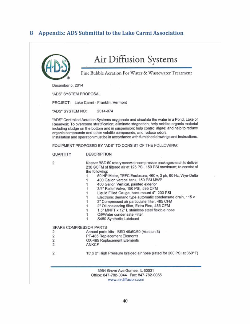
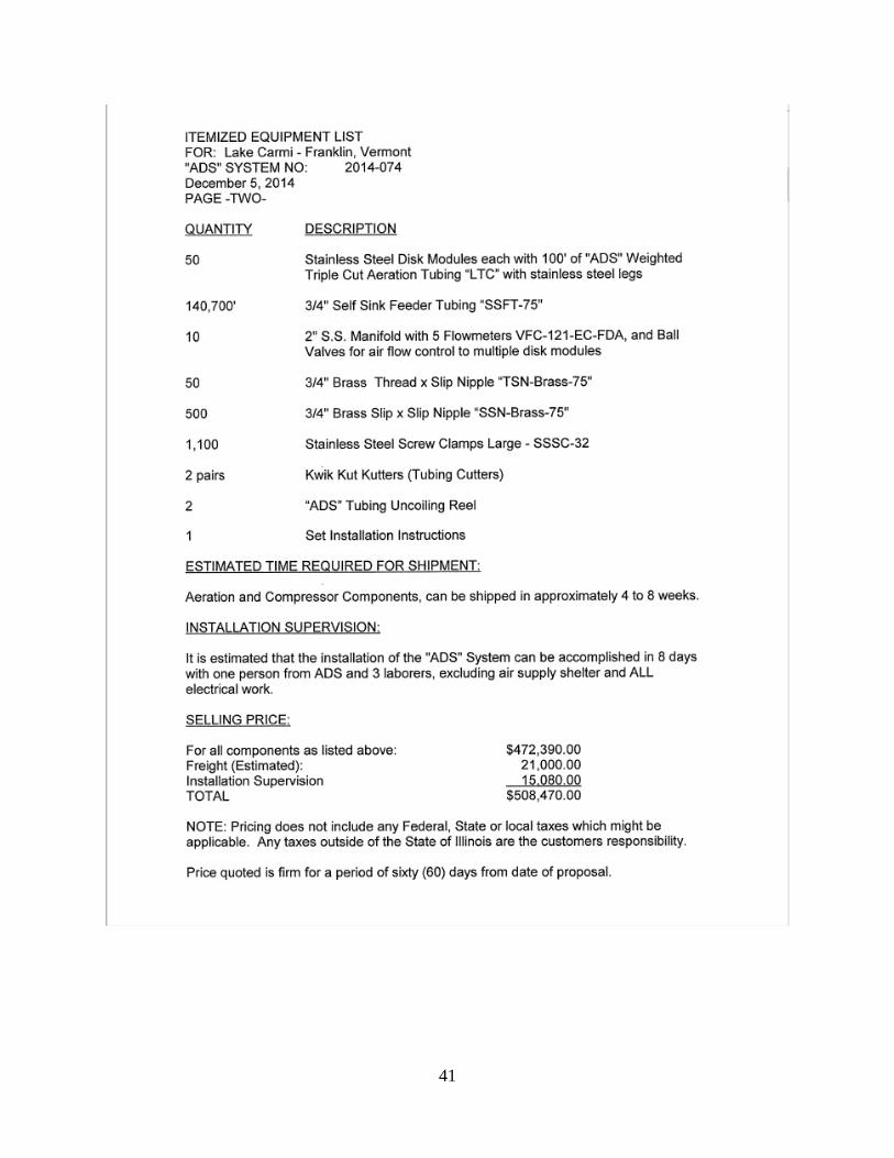
8 Appendix: ADS Submittal to the Lake Carmi Association ............................................................ 40

2

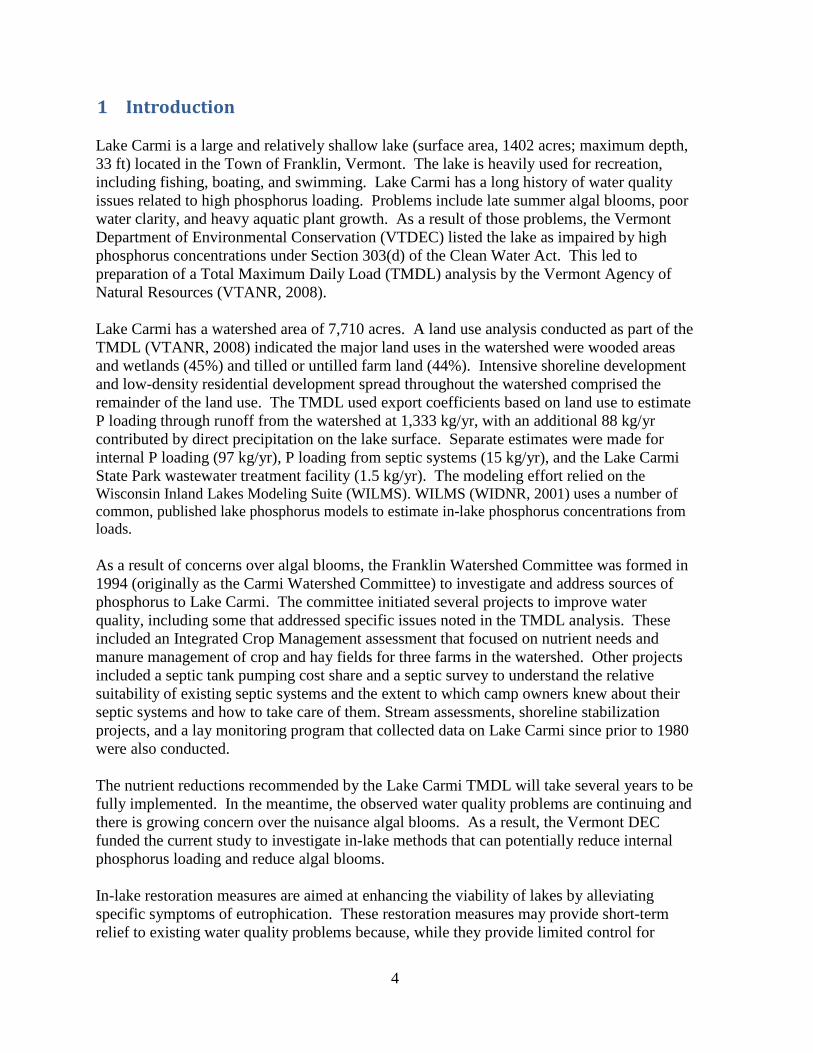
List of Figures Figure 2.1 - 2006 Modeled and Observed Temperature (top) and DO (bottom) Profiles in Lake Carmi. The x-axis is Temperature (oC) in the upper plots and DO (mg/L) in the lower plots, and the y-axis is Elevation (m). Depth to the bottom is about 9.5 m. Observed data are the circles, and modeled profiles are the lines (black, day of data collection; red, day before, and blue, day after). .................. 8

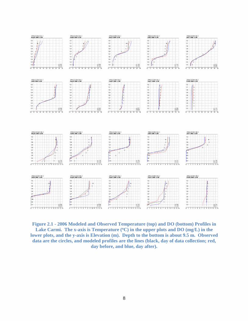
Figure 2.2 - 2007 Modeled and Observed Temperature (top) and DO (bottom) Profiles in Lake Carmi. The x-axis is Temperature (oC) in the upper plots and DO (mg/L) in the lower plots, and the y-axis is Elevation (m). Depth to the bottom is about 9.5 m. Observed data are the circles, and modeled profiles are the lines (black, day of data collection, red, day before, and blue, day after). .................. 9

Figure 2.3 - 2016 Modeled and Observed Temperature (top) and DO (bottom) Profiles in Lake Carmi. The x-axis is Temperature (oC) in the upper plots and DO (mg/L) in the lower plots, and the y-axis is Elevation (m). Depth to the bottom is about 8.5 m. Observed data are the circles, and modeled profiles are the lines (black, day of data collection, red, day before, and blue, day after). ................ 10

Figure 2.4 - 2017 Modeled and Observed Temperature (top) and DO (bottom) Profiles in Lake Carmi. The x-axis is Temperature (oC) in the upper plots and DO (mg/L) in the lower plots, and the y-axis is Elevation (m). Depth to the bottom is about 8.5 m. Observed data are the circles, and modeled profiles are the lines (black, day of data collection, red, day before, and blue, day after). ................ 11

Figure 2.5 – Model Predicted Dissolved Oxygen in Lake Carmi Without Added Inflow Phosphorus. . 12

Figure 2.6 – Model Predicted Dissolved Phosphorus in Lake Carmi Without Added Inflow Phosphorus. ......................................................................................................................................... 13

Figure 2.7 – Observed and Model Predicted Chlorophyll a Concentrations in Lake Carmi Without Added Inflow Phosphorus. These plots provide evidence that Cyanobacteria Can Use Buoyancy Control to Access Available Phosphorus Deep in the Water Column.................................................. 14

Figure 2.8 – Observed and Model Predicted Total Phosphorus Concentrations in Lake Carmi Without Added Inflow Phosphorus. ................................................................................................................... 15

Figure 2.9 – Model Predicted Dissolved Phosphorus in the Top Three Meters in Lake Carmi With (left) and Without (right) Added Inflow Phosphorus. .......................................................................... 16

Figure 2.10 – Model Predicted Chlorophyll a at 1.5 Meter Depth in Lake Carmi With and Without Added Phosphorus in the Inflow.......................................................................................................... 17

Figure 2.11 – Model Predicted Cyanobacteria and Total Algae at 1.5 Meter Depth in Lake Carmi With and Without Added Phosphorus in the Inflow. ................................................................................... 18

Figure 3.1 – Schematic of an MEI Line Diffuser (Top Figure) and Preliminary Layout of Line Diffuser in Lake Carmi (Bottom Figure). The diffuser shown along the bottom of the lake is about 5400 feet (1640 m). .............................................................................................................................................. 20

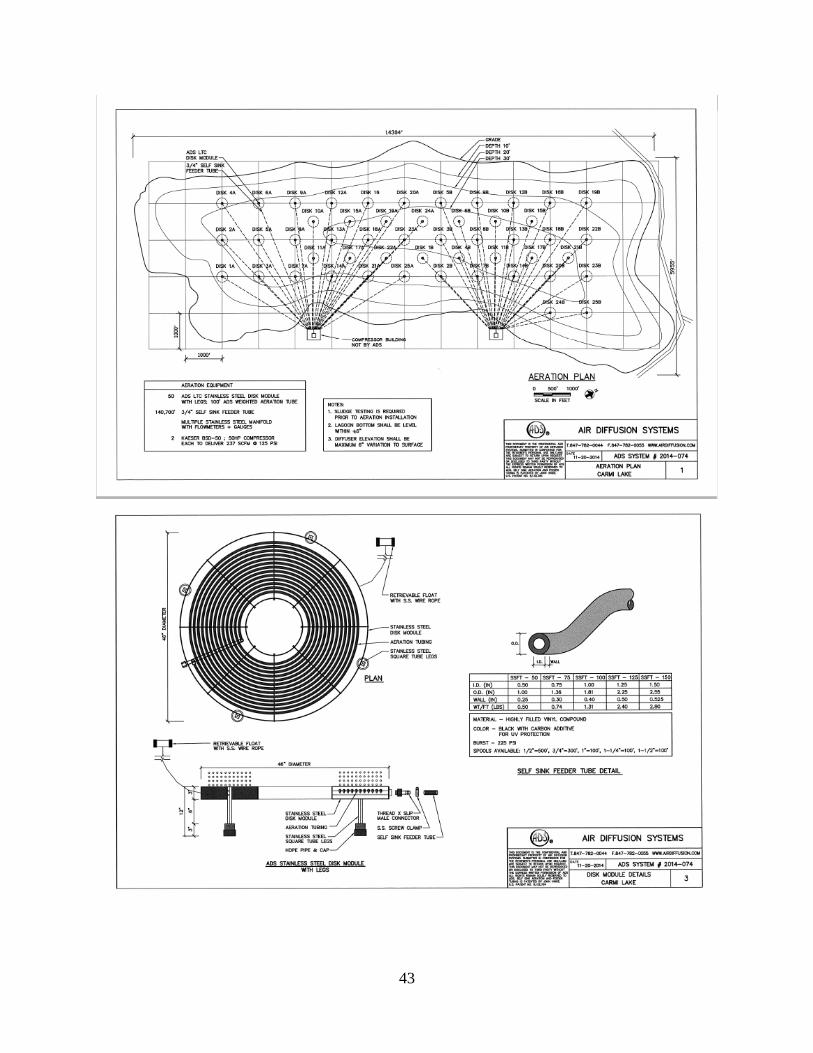
Figure 3.2 – ADS Disk Module (Top Figure) and Proposed Layout of Disks for Carmi Aeration (Bottom Figure) .................................................................................................................................................. 21

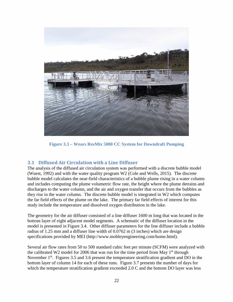
Figure 3.3 – Wears ResMix 5000 CC System for Downdraft Pumping ................................................. 22

Figure 3.4 - Model Bathymetry Showing Location of ResMix System and Location of Line Diffuser .. 23

Figure 3.5 - Temperature Stratification for a Line Diffuser with Several Air Flow Rates – 300 SCFM Provides Low Temperature Stratification with Reasonable System Size............................................. 24

3

Figure 3.6 - DO in the Bottom Model Layer for a Line Diffuser with Several Air Flow Rates -300 SCFM Provides High DO in Bottom Layer with Reasonable System Size ....................................................... 24

Figure 3.7 - Performance of Line Diffuser with Various Air Flow Rates ............................................... 25

Figure 3.8 - Temperature Stratification for Various Air Flow Rates and with Diffuser Operation Beginning on July 1st ............................................................................................................................. 25

Figure 3.9 - DO in the Bottom Model Layer for Various Air Flow Rates and with Diffuser Operation Beginning on July 1st ............................................................................................................................. 26

Figure 3.10 - Plume Flow Rates for a Disk diffuser and for a Line Diffuser with Two Different Ambient Temperature Profiles ........................................................................................................................... 29

Figure 3.11 - Plume Temperatures for a Disk diffuser and for a Line Diffuser with a Mixed Lake Temperature Profile ............................................................................................................................. 29

Figure 3.12 - Plume Temperatures for a Disk diffuser and for a Line Diffuser with an Unmixed Lake Temperature Profile ............................................................................................................................. 30

Figure 3.13 - Temperature Stratification at Two Different Model Locations for the ResMix System . 31

Figure 3.14 - DO in the Bottom Model Layer at Two Different Model Locations for the ResMix System ............................................................................................................................................................. 31

Figure 4.1 – Model Predicted Dissolved Oxygen in Lake Carmi With Mixing Starting on June 1. ....... 33

Figure 4.2 – Model Predicted Dissolved Phosphorus in Lake Carmi With Mixing Starting on June 1. 34

4

1 Introduction Lake Carmi is a large and relatively shallow lake (surface area, 1402 acres; maximum depth, 33 ft) located in the Town of Franklin, Vermont. The lake is heavily used for recreation, including fishing, boating, and swimming. Lake Carmi has a long history of water quality issues related to high phosphorus loading. Problems include late summer algal blooms, poor water clarity, and heavy aquatic plant growth. As a result of those problems, the Vermont Department of Environmental Conservation (VTDEC) listed the lake as impaired by high phosphorus concentrations under Section 303(d) of the Clean Water Act. This led to preparation of a Total Maximum Daily Load (TMDL) analysis by the Vermont Agency of Natural Resources (VTANR, 2008). Lake Carmi has a watershed area of 7,710 acres. A land use analysis conducted as part of the TMDL (VTANR, 2008) indicated the major land uses in the watershed were wooded areas and wetlands (45%) and tilled or untilled farm land (44%). Intensive shoreline development and low-density residential development spread throughout the watershed comprised the remainder of the land use. The TMDL used export coefficients based on land use to estimate P loading through runoff from the watershed at 1,333 kg/yr, with an additional 88 kg/yr contributed by direct precipitation on the lake surface. Separate estimates were made for internal P loading (97 kg/yr), P loading from septic systems (15 kg/yr), and the Lake Carmi State Park wastewater treatment facility (1.5 kg/yr). The modeling effort relied on the Wisconsin Inland Lakes Modeling Suite (WILMS). WILMS (WIDNR, 2001) uses a number of common, published lake phosphorus models to estimate in-lake phosphorus concentrations from loads. As a result of concerns over algal blooms, the Franklin Watershed Committee was formed in 1994 (originally as the Carmi Watershed Committee) to investigate and address sources of phosphorus to Lake Carmi. The committee initiated several projects to improve water quality, including some that addressed specific issues noted in the TMDL analysis. These included an Integrated Crop Management assessment that focused on nutrient needs and manure management of crop and hay fields for three farms in the watershed. Other projects included a septic tank pumping cost share and a septic survey to understand the relative suitability of existing septic systems and the extent to which camp owners knew about their septic systems and how to take care of them. Stream assessments, shoreline stabilization projects, and a lay monitoring program that collected data on Lake Carmi since prior to 1980 were also conducted. The nutrient reductions recommended by the Lake Carmi TMDL will take several years to be fully implemented. In the meantime, the observed water quality problems are continuing and there is growing concern over the nuisance algal blooms. As a result, the Vermont DEC funded the current study to investigate in-lake methods that can potentially reduce internal phosphorus loading and reduce algal blooms. In-lake restoration measures are aimed at enhancing the viability of lakes by alleviating specific symptoms of eutrophication. These restoration measures may provide short-term relief to existing water quality problems because, while they provide limited control for

5

nutrients and other pollutants, they can substantially improve the aesthetic and recreational potential of the lake and help gain public support for the restoration program while long-term management practices are being implemented. Wagner (2001) listed 18 potential in-lake management options, but those methods vary widely in cost, effectiveness in addressing various water quality problems, effects on other lake uses, and potential side effects. For example, chemical treatments can control nuisance algal growth but do not reduce nutrient concentrations and may have adverse long-term effects on other aquatic organisms. In contrast, dredging may reduce internal nutrient loading if enough nutrient rich-sediments can be removed, but it is expensive and is unlikely to control algal growth as long as significant external nutrient loading is occurring. Reservoir Environmental Management, Inc. (REMI) evaluated existing water quality data from Lake Carmi to determine the type of in-lake treatment that has the greatest probability of providing a cost-effective solution for improving lake water quality. Artificial mixing was identified as the most promising technique because it increases hypolimnetic dissolved oxygen concentrations to reduce internal phosphorus loading. Previous experience has shown that increased mixing can reduce cyanobacterial blooms. The two artificial mixing technologies deemed the most promising include diffused air circulation and downdraft pumping. The Phase 1 report recommended that model simulations be performed to gain additional insight into the water quality benefits of these techniques and to quantify their mixing performance. This report describes results of model simulations that include using a calibrated CE-QUAL-W2 (W2) model to evaluate the performance of a line diffuser and the performance of a downdraft pumping system. The simulation of the line diffuser is based on a preliminary design provided by Mobley Engineering, Inc. (MEI) during the Phase 1 study. The downdraft pumping simulation is based on a preliminary design of the WEARS ResMix System submitted during the Phase 1 study and then further modified based on email correspondence during this study. Additional simulations using a bubble plume model compare the performance of line diffusers to the performance of disk diffusers that are commercially available from Air Diffusion Systems (ADS) and were part of a proposal submitted by ADS in 2014.

2 Lake Carmi Water Quality Water quality monitoring has been carried out for Lake Carmi and its watershed through a variety of programs for over 40 years. Available water quality data for Lake Carmi is stored in the Vermont Integrated Watershed Information System (IWIS) and was summarized, along with various lake and watershed management measures that have been implemented to improve lake conditions, in a TMDL for Lake Carmi prepared by the Vermont Agency of Natural Resources (Vermont ANR, 2008). The TMDL reported mean concentrations of 28 µg/L for total phosphorus and 17 µg/L for chlorophyll a, with a mean Secchi depth of 2.0 m based on the 23-year period of record available at the time that document was prepared. Total phosphorus and chlorophyll a concentrations were higher, and Secchi depths were lower, in near-shore areas than in the center of the lake.

6

Based on a preliminary review of data available from IWIS, it appears that Lake Carmi experiences dissolved oxygen concentrations of less than 4 mg/L at depths of 6 m or more from approximately June through the fall overturn, which typically occurs in mid-September. During that period, iron concentrations increase in the hypolimnion of the lake and may be sufficient to bind with phosphorus that rarely exceeds hypolimnetic concentrations of 50 µg/L. Even if phosphorus removal is limited, beneficial changes in the algal community are still likely if an aeration/circulation project is initiated. Numerous previous studies have demonstrated that artificial circulation typically results in decreases in populations of cyanobacteria relative to other algal species. Nuisance algal blooms appear to be the primary concern for area residents. Walmsley and Butty (1979) proposed some typical relationships between maximum chlorophyll a concentrations and lake user perceptions of water quality. Chlorophyll a concentrations of 20-30 µg/L were indicative of nuisance conditions, while most lake users found that chlorophyll a concentrations of greater than 30 µg/L were indicative of severe nuisance conditions. The IWIS database shows that chlorophyll a concentrations greater than 20 µg/L have occurred in Lake Carmi as early as June, while concentrations greater than 30 µg/L occur most frequently in August and September. Area residents indicate the most severe algal blooms occur along the lake margins and particularly in the northeast corner of the lake (Vermont ANR, 2008). The most intensive monitoring was carried out in 1994-1996, 2006-2007, and 2016-2017. Those studies included profiles of phosphorus and other constituents. Profiles for temperature and dissolved oxygen from the 2006-2007 and 2016-2017 studies were used as the basis of the modeling conducted during this project. The W2 model was set up and calibrated to four years (2006, 2007, 2016 and 2017). The primary focus of the calibration was temperature, dissolved oxygen, total phosphorus and chlorophyll a. Figures 2.1 through 2.4 show the model-predicted temperature and DO profiles for the four years modeled compared to observed profiles from each year. Generally, the only model inputs that change with each year modeled are hydrology (i.e., inflow and outflow) and meteorology. All model coefficients were the same for all modeled years. Model calibration for each individual year could most likely be improved by adjusting the model coefficients, however, this was not attempted since temperature and DO dynamics in Lake Carmi were represented adequately for the objective of this modeling. Dissolved oxygen concentrations near the bottom were at or near zero for the entire months of July and August in all years modeled, and this anoxic period each year resulted in the release of phosphorus and iron from the sediments. Figure 2.5 presents time-series plots of model predicted DO throughout the water column for the four years modeled. Figure 2.6 presents time-series plots of model predicted dissolved phosphorus throughout the water column. These plots illustrate how anoxic conditions near the sediments result in the release of phosphorus.

7

During the calibration process it was determined that the models had a tendency to under-predict chlorophyll a concentrations in Lake Carmi. This bias was exposed by comparing the model-predicted chlorophyll a at 1.5 meters depth to chlorophyll a measurements from the year modeled as well as chlorophyll a data collected in 1991-2017. Figure 2.5 shows the model-predicted chlorophyll a at 1.5 meters depth for the four years modeled along with historical observations. As shown in the plots the model predicted concentrations do not reach the peaks that typically occur in Lake Carmi, especially in August. Figure 2.6 shows the model-predicted total phosphorus concentrations at 1.5 meter depth for all years modeled along with historical observations. These plots show that phosphorus concentrations predicted by the model are consistent with measured concentrations. Since model-predicted phosphorus concentrations near the surface represented actual concentrations in Lake Carmi, it was concluded that cyanobacteria are using buoyancy to access phosphorus that is available deeper in the water column (see Figure 2.6). Cyanobacteria, that are typically dominant in Lake Carmi during late-summer, have the capability to use buoyancy to drop in the water column to access phosphorus and then return to shallower depths where light is available. Because this phenomenon was not modeled, the cyanobacteria were under-predicted. To test this hypothesis, the phosphorus concentration in the inflow to the Lake Carmi W2 model was doubled to see if chlorophyll a concentrations near the surface increased, and therefore, better matched the observed data. Figure 2.9 shows the model-predicted dissolved phosphorus concentrations with and without the added phosphorus in the inflow for the four years modeled. Although the increase is phosphorus appears minor, the effect on chlorophyll a concentrations is obvious. Figure 2.10 shows the comparison of the model-predicted chlorophyll a at 1.5 meters for the four years modeled for the cases with and without added phosphorus in the inflow. Although agreement between the model predicted and observed concentrations are not ideal, the results illustrate that algal growth in Lake Carmi depends on availability of relatively high concentrations of phosphorus that occur deeper in the water column. Figure 2.11 presents time-series plots of cyanobacteria and total algae for the four years modeled. These plots show the effect that added availability of additional phosphorus has on algae concentrations near the surface.

8

Figure 2.1 - 2006 Modeled and Observed Temperature (top) and DO (bottom) Profiles in Lake Carmi. The x-axis is Temperature (oC) in the upper plots and DO (mg/L) in the

lower plots, and the y-axis is Elevation (m). Depth to the bottom is about 9.5 m. Observed data are the circles, and modeled profiles are the lines (black, day of data collection; red,

day before, and blue, day after).

9

Figure 2.2 - 2007 Modeled and Observed Temperature (top) and DO (bottom) Profiles in

Lake Carmi. The x-axis is Temperature (oC) in the upper plots and DO (mg/L) in the lower plots, and the y-axis is Elevation (m). Depth to the bottom is about 9.5 m. Observed data are the circles, and modeled profiles are the lines (black, day of data collection, red,


10


lower plots, and the y-axis is Elevation (m). Depth to the bottom is about 8.5 m. Observed data are the circles, and modeled profiles are the lines (black, day of data collection, red,


11


lower plots, and the y-axis is Elevation (m). Depth to the bottom is about 8.5 m. Observed data are the circles, and modeled profiles are the lines (black, day of data collection, red,


12

Figure 2.5 – Model Predicted Dissolved Oxygen in Lake Carmi Without Added Inflow Phosphorus.

0

1

2

3

4

5

6

7

8

9

10

11

12

13

14

5/1 5/11 5/21 5/31 6/10 6/20 6/30 7/10 7/20 7/30 8/9 8/19 8/29 9/8 9/18 9/28 10/8 10/18 10/28

Conc

entr

atio

n (m

g/L)

Date

2006 Dissolved Oxygen

1m

2m

3m

4m

5m

6m

7m

Bottom0

1

2

3

4

5

6

7

8

9

10

11

12

13

14

5/1 5/11 5/21 5/31 6/10 6/20 6/30 7/10 7/20 7/30 8/9 8/19 8/29 9/8 9/18 9/28 10/8 10/18 10/28

Conc

entr

atio

n (m

g/L)

Date


1m

2m

3m

4m

5m

6m

7m

Bottom

0

1

2

3

4

5

6

7

8

9

10

11

12

13

14

5/1 5/11 5/21 5/31 6/10 6/20 6/30 7/10 7/20 7/30 8/9 8/19 8/29 9/8 9/18 9/28 10/8 10/18 10/28

Conc

entr

atio

n (m

g/L)

Date


1m

2m

3m

4m

5m

6m

7m

Bottom0

1

2

3

4

5

6

7

8

9

10

11

12

13

14

5/1 5/11 5/21 5/31 6/10 6/20 6/30 7/10 7/20 7/30 8/9 8/19 8/29 9/8 9/18 9/28 10/8 10/18 10/28

Conc

entr

atio

n (m

g/L)

Date


1m

2m

3m

4m

5m

6m

7m

Bottom

13

Figure 2.6 – Model Predicted Dissolved Phosphorus in Lake Carmi Without Added Inflow Phosphorus.

0.000.010.020.030.040.050.060.070.080.090.100.110.120.130.140.150.16

5/1 5/11 5/21 5/31 6/10 6/20 6/30 7/10 7/20 7/30 8/9 8/19 8/29 9/8 9/18 9/28 10/8 10/18 10/28

Conc

entr

atio

n (m

g/L)

Date

2006 Dissolved Phosphorus

1m

2m

3m

4m

5m

6m

7m

Bottom

0.000.010.020.030.040.050.060.070.080.090.100.110.120.130.140.150.16

5/1 5/11 5/21 5/31 6/10 6/20 6/30 7/10 7/20 7/30 8/9 8/19 8/29 9/8 9/18 9/28 10/8 10/18 10/28

Conc

entr

atio

n (m

g/L)

Date


1m

2m

3m

4m

5m

6m

7m

Bottom

0.000.010.020.030.040.050.060.070.080.090.100.110.120.130.140.150.16

5/1 5/11 5/21 5/31 6/10 6/20 6/30 7/10 7/20 7/30 8/9 8/19 8/29 9/8 9/18 9/28 10/8 10/18 10/28

Conc

entr

atio

n (m

g/L)

Date


1m

2m

3m

4m

5m

6m

7m

Bottom

0.000.010.020.030.040.050.060.070.080.090.100.110.120.130.140.150.16

5/1 5/11 5/21 5/31 6/10 6/20 6/30 7/10 7/20 7/30 8/9 8/19 8/29 9/8 9/18 9/28 10/8 10/18 10/28

Conc

entr

atio

n (m

g/L)

Date


1m

2m

3m

4m

5m

6m

7m

Bottom

14

Figure 2.7 – Observed and Model Predicted Chlorophyll a Concentrations in Lake Carmi Without Added Inflow Phosphorus.

These plots provide evidence that Cyanobacteria Can Use Buoyancy Control to Access Available Phosphorus Deep in the Water Column

0

10

20

30

40

50

60

70

80

90

100

110

5/1 5/11 5/21 5/31 6/10 6/20 6/30 7/10 7/20 7/30 8/9 8/19 8/29 9/8 9/18 9/28 10/8 10/18 10/28

Conc

entr

atio

n (u

g/L)

Date

2006 Chlorophyll a - 1.5 Meter

1980-2016 Observations

2006 Observations

Model Predicted at 1.5m

0

10

20

30

40

50

60

70

80

90

100

110

5/1 5/11 5/21 5/31 6/10 6/20 6/30 7/10 7/20 7/30 8/9 8/19 8/29 9/8 9/18 9/28 10/8 10/18 10/28

Conc

entr

atio

n (u

g/L)

Date



2007 Observations


0

10

20

30

40

50

60

70

80

90

100

110

5/1 5/11 5/21 5/31 6/10 6/20 6/30 7/10 7/20 7/30 8/9 8/19 8/29 9/8 9/18 9/28 10/8 10/18 10/28

Conc

entr

atio

n (u

g/L)

Date



2016 Observations


0

10

20

30

40

50

60

70

80

90

100

110

5/1 5/11 5/21 5/31 6/10 6/20 6/30 7/10 7/20 7/30 8/9 8/19 8/29 9/8 9/18 9/28 10/8 10/18 10/28Co

ncen

trat

ion

(ug/

L)Date



2017 Observations


15

Figure 2.8 – Observed and Model Predicted Total Phosphorus Concentrations in Lake Carmi Without Added Inflow

Phosphorus.

0.00

0.02

0.04

0.06

0.08

0.10

0.12

0.14

0.16

0.18

0.20

3/25 4/9 4/24 5/9 5/24 6/8 6/23 7/8 7/23 8/7 8/22 9/6 9/21 10/6 10/21 11/5 11/20

Conc

entr

atio

n (m

g/L)

Date

2006 Total Phosphorus


2006 Observations

Model Predicted - 1.5m

0.00

0.02

0.04

0.06

0.08

0.10

0.12

0.14

0.16

0.18

0.20

3/25 4/9 4/24 5/9 5/24 6/8 6/23 7/8 7/23 8/7 8/22 9/6 9/21 10/6 10/21 11/5 11/20

Conc

entr

atio

n (u

g/L)

Date

2007 Total Phosphorus - 1.5 Meter


2007 Observations

Model Predicted 1.5m

0.00

0.02

0.04

0.06

0.08

0.10

0.12

0.14

0.16

0.18

0.20

3/25 4/9 4/24 5/9 5/24 6/8 6/23 7/8 7/23 8/7 8/22 9/6 9/21 10/6 10/21 11/5 11/20

Conc

entr

atio

n (m

g/L)

Date



2016 Observations

1.5 meter

0.00

0.02

0.04

0.06

0.08

0.10

0.12

0.14

0.16

0.18

0.20

3/25 4/9 4/24 5/9 5/24 6/8 6/23 7/8 7/23 8/7 8/22 9/6 9/21 10/6 10/21 11/5 11/20Co

ncen

trat

ion

(mg/

L)Date



Model Predicted 1.5m

16

Figure 2.9 – Model Predicted Dissolved Phosphorus in the Top Three Meters in Lake Carmi With (left) and Without (right) Added Inflow Phosphorus.

0.000

0.005

0.010

0.015

0.020

0.025

0.030

0.035

0.040

0.045

0.050

5/1 5/11 5/21 5/31 6/10 6/20 6/30 7/10 7/20 7/30 8/9 8/19 8/29 9/8 9/18 9/28 10/8 10/18 10/28

Conc

entr

atio

n (m

g/L)

Date


1m

2m

3m

0.000

0.005

0.010

0.015

0.020

0.025

0.030

0.035

0.040

0.045

0.050

5/1 5/11 5/21 5/31 6/10 6/20 6/30 7/10 7/20 7/30 8/9 8/19 8/29 9/8 9/18 9/28 10/8 10/18 10/28

Conc

entr

atio

n (m

g/L)

Date


1m

2m

3m

0.000

0.005

0.010

0.015

0.020

0.025

0.030

0.035

0.040

0.045

0.050

5/9 5/19 5/29 6/8 6/18 6/28 7/8 7/18 7/28 8/7 8/17 8/27 9/6 9/16 9/26 10/6 10/16 10/26 11/5

Conc

entr

atio

n (m

g/L)

Date


1m

2m

3m

0.000

0.005

0.010

0.015

0.020

0.025

0.030

0.035

0.040

0.045

0.050

5/1 5/11 5/21 5/31 6/10 6/20 6/30 7/10 7/20 7/30 8/9 8/19 8/29 9/8 9/18 9/28 10/8 10/18 10/28

Conc

entr

atio

n (m

g/L)

Date


1m

2m

3m

0.000

0.005

0.010

0.015

0.020

0.025

0.030

0.035

0.040

0.045

0.050

5/9 5/19 5/29 6/8 6/18 6/28 7/8 7/18 7/28 8/7 8/17 8/27 9/6 9/16 9/26 10/6 10/16 10/26 11/5

Conc

entr

atio

n (m

g/L)

Date


1m

2m

3m

0.000

0.005

0.010

0.015

0.020

0.025

0.030

0.035

0.040

0.045

0.050

5/1 5/11 5/21 5/31 6/10 6/20 6/30 7/10 7/20 7/30 8/9 8/19 8/29 9/8 9/18 9/28 10/8 10/18 10/28

Conc

entr

atio

n (m

g/L)

Date


1m

2m

3m

0.000

0.005

0.010

0.015

0.020

0.025

0.030

0.035

0.040

0.045

0.050

5/9 5/19 5/29 6/8 6/18 6/28 7/8 7/18 7/28 8/7 8/17 8/27 9/6 9/16 9/26 10/6 10/16 10/26 11/5

Conc

entr

atio

n (m

g/L)

Date


1m

2m

3m

0.000

0.005

0.010

0.015

0.020

0.025

0.030

0.035

0.040

0.045

0.050

5/1 5/11 5/21 5/31 6/10 6/20 6/30 7/10 7/20 7/30 8/9 8/19 8/29 9/8 9/18 9/28 10/8 10/18 10/28

Conc

entr

atio

n (m

g/L)

Date


1m

2m

3m

17

Figure 2.10 – Model Predicted Chlorophyll a at 1.5 Meter Depth in Lake Carmi With and Without Added Phosphorus in the

Inflow.

0

10

20

30

40

50

60

70

80

90

100

110

5/1 5/11 5/21 5/31 6/10 6/20 6/30 7/10 7/20 7/30 8/9 8/19 8/29 9/8 9/18 9/28 10/8 10/18 10/28

Conc

entr

atio

n (u

g/L)

Date


2006 Observations

With Additional Phosphorus added in the Inflow

Without Additional Phosphorus in the Inflow

0

10

20

30

40

50

60

70

80

90

100

110

5/1 5/11 5/21 5/31 6/10 6/20 6/30 7/10 7/20 7/30 8/9 8/19 8/29 9/8 9/18 9/28 10/8 10/18 10/28

Conc

entr

atio

n (u

g/L)

Date


2007 Observations

With Additional Phosphorus Added in the Inflow

Without Additional Phosphorus Added in the Inflow

0

10

20

30

40

50

60

70

80

90

100

110

5/1 5/11 5/21 5/31 6/10 6/20 6/30 7/10 7/20 7/30 8/9 8/19 8/29 9/8 9/18 9/28 10/8 10/18 10/28

Conc

entr

atio

n (u

g/L)

Date


2016 Observations

With Additional Phosphorus in the Inflow

Without Additional Phosphorus in the Inflow

0

10

20

30

40

50

60

70

80

90

100

110

5/1 5/11 5/21 5/31 6/10 6/20 6/30 7/10 7/20 7/30 8/9 8/19 8/29 9/8 9/18 9/28 10/8 10/18 10/28Co

ncen

trat

ion

(ug/

L)

Date


2017 Observations

With Phosphorus Added to the Inflow

Without Phosphorus Added to the Inflow

18

Figure 2.11 – Model Predicted Cyanobacteria and Total Algae at 1.5 Meter Depth in Lake Carmi With and Without Added

Phosphorus in the Inflow.

0

1

2

3

4

5

6

7

8

9

10

11

12

13

14

5/1 5/16 5/31 6/15 6/30 7/15 7/30 8/14 8/29 9/13 9/28 10/13 10/28

Conc

entr

atio

n (m

g/L)

Date

2006 Model-Predicted Cyanobacteria and Total Algae

Cyanobacteria With Additional Phosphorus in the Inflow

Total Algae with Additional Phosphorus in the Inflow

Cyanobacteria Without Additional Phosphorus in the Inflow

Total Algae Without Additional Phosphorus in the Inflow

0

1

2

3

4

5

6

7

8

9

10

11

12

13

14

5/1 5/16 5/31 6/15 6/30 7/15 7/30 8/14 8/29 9/13 9/28 10/13 10/28

Conc

entr

atio

n (m

g/L)

Date






0

1

2

3

4

5

6

7

8

9

10

11

12

13

14

5/1 5/16 5/31 6/15 6/30 7/15 7/30 8/14 8/29 9/13 9/28 10/13 10/28

Conc

entr

atio

n (m

g/L)

Date






0

1

2

3

4

5

6

7

8

9

10

11

12

13

14

5/1 5/16 5/31 6/15 6/30 7/15 7/30 8/14 8/29 9/13 9/28 10/13 10/28

Conc

entr

atio

n (m

g/L)

Date






19

3 Mixing Analyses Three mixing techniques were evaluated: diffused air circulation with a line diffuser (Figure 3.1), diffused air circulation with disk diffusers (Figure 3.2), and downdraft pumping (Figure 3.3). Line diffusers and downdraft pumping were compared with near-field models that were operated in conjunction with CE-QUAL-W2 (W2) to compute the far-field effects of the mixing techniques. The disk diffusers were compared to the line diffusers by comparing plume flow rates and plume temperatures, computed with a bubble plume model (Wuest, 1992), for the two diffuser geometries and for different temperature profiles. The performance of the diffusers was based on two metrics that include the vertical temperature gradient and DO in the bottom model layer. The vertical temperature gradient is computed by subtracting the temperature of the bottom layer of the model from the temperature of the third model layer below the water surface (1.25 m deep), at a given column of the model. Using a layer that is a few feet below the surface eliminates diurnal fluctuations in temperature and yields a clearer indication of the mixing effectiveness. The amount of time that the temperature stratification exceeds 2.0 C is also presented for a few analyses to summarize the time series results. A quantitative measure of the vertical temperature gradient is useful to compare the relative effectiveness of mixing techniques. The two components required for quantifying the effectiveness of mixing include the magnitude of the vertical temperature gradient and the time over which the temperature gradient occurred. For this study the metric that was chosen is the number of days that the vertical temperature exceeded two degrees C. Although there are no studies specifying two degrees C as an acceptable degree of mixing, it was chosen because two degrees represents a low summer vertical temperature gradient (and high level of mixing) and is straightforward to comprehend when expressed as the number of days. An alternate metric that quantifies mixing is degree days, but the units of degree days are somewhat obscure and not used for this reason. The second indicator was the DO in the bottom layer of the model. This is an important measure of mixing effectiveness because eliminating anoxic conditions in the hypolimnion of a lake can eliminate internal phosphorus release from the sediments. Time series of DO in the bottom layer are presented for each mixing technique and the quantity of time when the DO in the bottom layer exceeds 2.0 mg/l is computed to summarize the time series results.

20

Figure 3.1 – Schematic of an MEI Line Diffuser (Top Figure) and Preliminary Layout of Line Diffuser in Lake Carmi (Bottom Figure). The diffuser shown along the bottom of the

lake is about 5400 feet (1640 m).

21

Figure 3.2 – ADS Disk Module (Top Figure) and Proposed Layout of Disks for Carmi

Aeration (Bottom Figure)

22

Figure 3.3 – Wears ResMix 5000 CC System for Downdraft Pumping

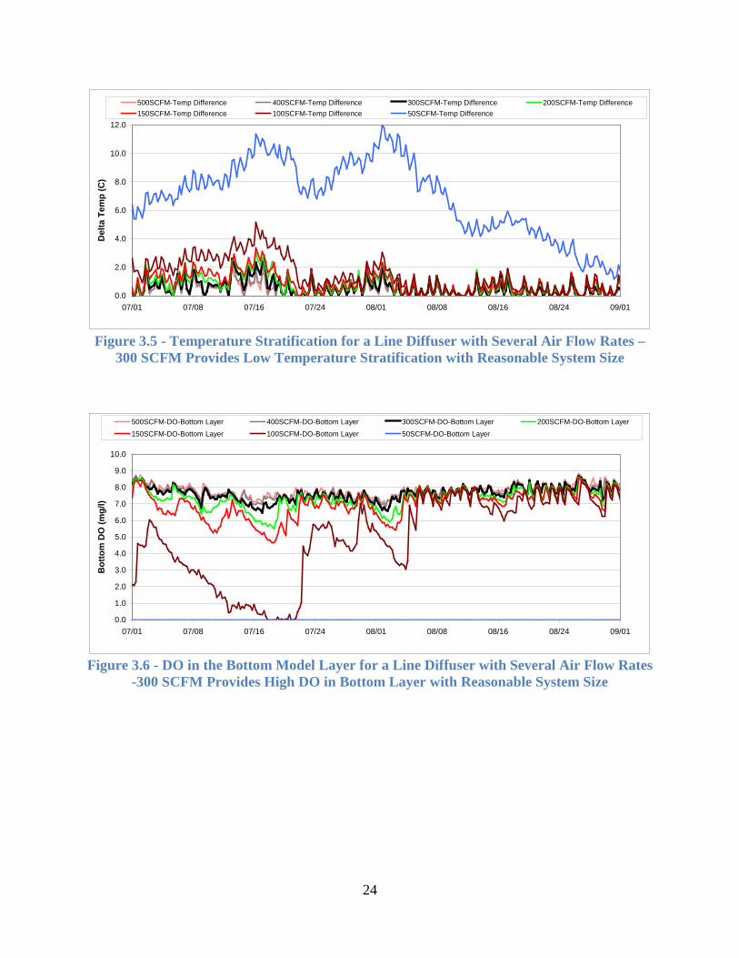
3.1 Diffused Air Circulation with a Line Diffuser The analysis of the diffused air circulation system was performed with a discrete bubble model (Wuest, 1992) and with the water quality program W2 (Cole and Wells, 2015). The discrete bubble model calculates the near-field characteristics of a bubble plume rising in a water column and includes computing the plume volumetric flow rate, the height where the plume detrains and discharges to the water column, and the air and oxygen transfer that occurs from the bubbles as they rise in the water column. The discrete bubble model is integrated in W2 which computes the far field effects of the plume on the lake. The primary far field effects of interest for this study include the temperature and dissolved oxygen distribution in the lake. The geometry for the air diffuser consisted of a line diffuser 1600 m long that was located in the bottom layer of eight adjacent model segments. A schematic of the diffuser location in the model is presented in Figure 3.4. Other diffuser parameters for the line diffuser include a bubble radius of 1.25 mm and a diffuser line width of 0.0762 m (3 inches) which are design specifications provided by MEI (http://www.mobleyengineering.com/home.html). Several air flow rates from 50 to 500 standard cubic feet per minute (SCFM) were analyzed with the calibrated W2 model for 2006 that was run for the time period from May 1st through November 1st. Figures 3.5 and 3.6 present the temperature stratification gradient and DO in the bottom layer of column 14 for each of these runs. Figure 3.7 presents the number of days for which the temperature stratification gradient exceeded 2.0 C and the bottom DO layer was less

23

than 2.0 mg/l. An air flow rate of 300 SCFM provides a reasonable tradeoff between air flow rate (which will affect system size and cost) and the mixing performance. As air flow rate increases above 300 SCFM the number of days that the temperature stratification exceeds 2.0 C is not strongly affected, while decreasing the air flow rate below 300 SCFM does increase the temperature stratification and decrease the bottom DO. An additional metric useful for evaluating mixing performance is the time it takes to mix a lake after the system has fully stratified. Figures 3.8 and 3.9 present the temperature stratification and the DO in the bottom layer in column 14 of the model for runs of various flow rates when the diffuser operation was started on July 1st after the lake was fully stratified. These plots show that there is a significant improvement in diffuser performance by increasing the air flow rate from 200 to 300 SCFM. The DO in the bottom layer increases above 2.0 mg/l almost immediately for the 300 SCFM air flow rate but requires over 20 days with an air flow rate of 200 SCFM. The improvements in performance are smaller as the air flow rate increases above 300 SCFM.

Figure 3.4 - Model Bathymetry Showing Location of ResMix System and Location of Line

Diffuser

24

Figure 3.5 - Temperature Stratification for a Line Diffuser with Several Air Flow Rates –

300 SCFM Provides Low Temperature Stratification with Reasonable System Size

Figure 3.6 - DO in the Bottom Model Layer for a Line Diffuser with Several Air Flow Rates

-300 SCFM Provides High DO in Bottom Layer with Reasonable System Size

Temp Stratification

0.0

2.0

4.0

6.0

8.0

10.0

12.0

07/01 07/08 07/16 07/24 08/01 08/08 08/16 08/24 09/01

Del

ta T

emp

(C)

500SCFM-Temp Difference 400SCFM-Temp Difference 300SCFM-Temp Difference 200SCFM-Temp Difference150SCFM-Temp Difference 100SCFM-Temp Difference 50SCFM-Temp Difference

Bottom DO

0.0

1.0

2.0

3.0

4.0

5.0

6.0

7.0

8.0

9.0

10.0

07/01 07/08 07/16 07/24 08/01 08/08 08/16 08/24 09/01

Bot

tom

DO

(mg/

l)

500SCFM-DO-Bottom Layer 400SCFM-DO-Bottom Layer 300SCFM-DO-Bottom Layer 200SCFM-DO-Bottom Layer150SCFM-DO-Bottom Layer 100SCFM-DO-Bottom Layer 50SCFM-DO-Bottom Layer

25

Figure 3.7 - Performance of Line Diffuser with Various Air Flow Rates

Figure 3.8 - Temperature Stratification for Various Air Flow Rates and with Diffuser

Operation Beginning on July 1st

0

20

40

60

80

100

120

140

0 50 100 150 200 300 400 500

Air Flow Rate (SCFM)

Num

ber o

f Day

s

Temp Stratification Exceeds 2.0 C

DO in Bottom Layer Less Than 2.0 mg/l

Temp Stratification

0.0

2.0

4.0

6.0

8.0

10.0

12.0

14.0

16.0

06/01 06/08 06/16 06/24 07/02 07/09 07/17 07/25 08/02 08/09 08/17 08/25 09/02

Del

ta T

emp

(C)

BaseCase-Temp Difference AirDiff200-Temp Difference AirDiff300-Temp Difference

AirDiff400-Temp Difference AirDiff500-Temp Difference

26

Figure 3.9 - DO in the Bottom Model Layer for Various Air Flow Rates and with Diffuser

Operation Beginning on July 1st

3.2 Diffused Air Circulation with Disk Diffusers An alternate configuration for an air diffuser is with a line diffuser configured in a spiral to create a circular plume (Figure 3.2)—see Section 8 ADS submittal to The Lake Carmi Association. This configuration is commercially available from ADS and will subsequently be referred to as a disk diffuser. A comparison between a line diffuser and a disk diffuser was performed by using BPi (Loginetics) which implements a bubble plume model (Wuest, 1992) and has the capability to model both line diffusers and circular plumes from disk diffusers of various configurations and for various ambient conditions. The bubble plume model used in BPi is identical to the model used in the W2 simulations. Plume flow rates were compared between a disk diffuser and a line diffuser for two different cases. These cases include: 1) a temperature profile for July 15th from a W2 model run that included continuous mixing with an air flow rate of 300 SCFM (mixed profile); and 2) a temperature profile for July 15th from a W2 model run without artificial mixing (unmixed profile). A temperature profile on July 15th was chosen because it represents a highly stratified reservoir, typical of the current conditions, and the mixed conditions for July 15th represent typical model predicted conditions with continual operation of a mixing system. The disk diffuser was configured to be 1.2 m in diameter with an air flow rate of 8.1 SCFM and a bubble radius of 1.25 mm. The line diffuser was configured to be 43.2 m with an air flow rate of 8.1 SCFM. This configuration for the line diffuser produces the same flux of 0.188 SCFM/m as the 1600 m line diffuser with the recommended air flow rate of 300 SCFM. A comparison between the plume flow rates for the two types of diffusers is presented in Figure 3.10. The range of plume flow rates produced by the disk diffuser is approximately the same at 2.5 and 2.6 cms for each of the temperature profiles. The range of plume flow rates for the line diffuser varies between 4.4 and 6.6 cms for the unmixed and mixed profiles. The plume flow rates of the line diffusers are 2.5 and 1.7 times larger than the plume flow rates for the disk diffusers for the mixed and unmixed lake temperature profiles.

Bottom DO

0.0

1.0

2.0

3.0

4.0

5.0

6.0

7.0

8.0

9.0

10.0

06/01 06/08 06/16 06/24 07/02 07/09 07/17 07/25 08/02 08/09 08/17 08/25 09/02

Bot

tom

DO

(mg/

l)BaseCase-DO-Bottom Layer AirDiff200-DO-Bottom Layer AirDiff300-DO-Bottom Layer

AirDiff400-DO-Bottom Layer AirDiff500-DO-Bottom Layer

27

The plume for the line diffuser in the unmixed lake experiences several detrainments during which the plume stops, discharges to the water column at the level of detrainment, and then starts upward again as the bubbles continue to rise. The plume for the disk diffuser has one detrainment for the unmixed lake and no detrainments for the mixed lake. A detrainment occurs when the upward momentum of the plume and the positive buoyancy force of the bubbles cannot overcome the force from the negative buoyancy created by the density (and temperature) difference between the plume and the ambient water. The negative buoyancy becomes larger with increasing stratification because the plume continually entrains cool water from lower depths. When the plume detrains, it discharges to the water column. The air bubbles then continue to rise, they entrain water, and another plume is created. This process continues until either the plume reaches the surface of the lake, or the air bubbles completely dissolve. The size of the air bubbles in a mixing diffuser is typically large enough that they do not completely dissolve. The line diffuser has more entrainments because the surface area of the plume is larger than the surface area of the plume for the disk diffuser and it entrains more water. And as described above, the larger plume volume creates a larger downwardly buoyant force, which leads to a larger number of detrainments for the line diffuser plume. The mixing effect of a plume on a lake depends on both the flow rate of the plume and the temperature difference between the plume and the lake level where it detrains. Because the objective of an upwelling system is to mix the cooler water near the bottom of the reservoir with the warmer water near the surface, the cooling rate that the plume provides is an objective measure of the mixing performance. The cooling rate will subsequently be referred to as the mixing rate. The mixing rate of a plume on the layer to which it discharges is quantified with the following equation:

𝑞𝑞 = 𝑚𝑚 ∗ 𝑐𝑐𝑐𝑐 ∗ 𝜌𝜌 ∗ (𝑇𝑇𝑐𝑐 − 𝑇𝑇𝑇𝑇) where

q = mixing rate (J/s) m = plume flow rate (cms) cp = heat capacity (kJ/kg C) Tp = plume temperature (C) Ta = lake temperature where plume detrains (C)

The total mixing rate for a plume is computed by summing the effects of each detrainment, including the discharge to the surface layer. Figure 3.11 presents the plume and ambient temperatures for the mixed profile. The plume temperatures for both the line diffuser and disk diffuser are nearly the same, with the exception of the temperature deviation near the surface. The plume for the line diffuser detrains near the surface while the plume for the disk diffuser rises to the surface. The mixing rate for the line diffuser is computed by combining the effect of the two detrainments. The plume flow rate of the first detrainment is 6.2 cms with a temperature difference of 1.6 C between the plume and ambient water. The plume flow rate for the second detrainment is 6.6 cms with a temperature difference of 0.04 C. The combined mixing rate for both of these detrainments is 42.5 kJ/s. Computing the mixing rate for the disk diffuser results in a mixing rate of 15.8 kJ/s (plume flow

28

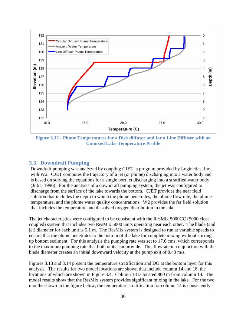
rate of 2.7 cms and temperature difference of 1.4 C). For the case of the mixed lake, the mixing rate of the line diffuser is 2.7 times larger than the disk diffuser. Figure 3.12 compares the plume temperatures for the two diffusers in the unmixed lake and shows that the plume dynamics are different for the two diffusers. The plume for the line diffuser undergoes several detrainments with small temperature differences between the plume and ambient water while the disk diffuser detrains once and then rises to the surface. Using the same approach as described above to compute mixing rates results in a mixing rate of 122.7 kJ/s for the line diffuser as compared to 83.6 kJ/s for the disk diffuser. For the case of the unmixed lake the mixing rate of the line diffuser is 1.5 times larger than the mixing rate for the disk diffuser. A phenomena not included in this calculation is the fallback of the plume. As the plume discharges to the lake, it will flow downward and continue to mix with the ambient water until the temperature (and density) between the plume discharge and lake are in equilibrium. The fallback region increases as the temperature difference between the plume and the ambient water increases. Because the plume for the disk diffuser is much cooler than the ambient water it will fall back to a greater depth than the line diffuser, thereby further decreasing the mixing rate. Because both the line diffuser and disk diffuser systems are uniformly distributed throughout the lake, the W2 modeling results and scaling relationships can be used to compare the performance of the two systems. The W2 analysis showed that an air flow rate of 300 SCFM provides effective mixing for both an unmixed and mixed lake. The ADS disk diffusers provide 8.1 SCFM per disk. Therefore 37 disk diffusers would be required to provide the same air flow rate as the line diffuser. The analyses above showed that the mixing rate of a line diffuser was between 1.5 and 2.7 times higher than a disk diffuser for the unmixed and mixed lake conditions. Therefore, the number of disks required to provide an equivalent mixing rate as the line diffuser is between 56 (37 x 1.5) and 100 (37 x 2.7) disk diffusers for the unmixed and mixed lake conditions, respectively.

29

Figure 3.10 - Plume Flow Rates for a Disk diffuser and for a Line Diffuser with Two

Different Ambient Temperature Profiles

Figure 3.11 - Plume Temperatures for a Disk diffuser and for a Line Diffuser with a Mixed

Lake Temperature Profile

122

123

124

125

126

127

128

129

130

131

132

0.0 1.0 2.0 3.0 4.0 5.0 6.0 7.0 8.0

Plume Flow Rate (cms)

Elev

atio

n (m

)0

1

2

3

4

5

6

7

8

9

10

Dep

th (m

)Circular Plume, July 15 Temp ProfileCircular Plume, Constant Temp of 20 CCircular Plume, Linear Temp ProfileCircular Plume, July 15 w 300 SCFM AirLD July 15 Temp ProfileLD Linear Temp ProfileLD July 15 w 300 SCFM Air LD Constant Temp of 20 C

122

123

124

125

126

127

128

129

130

131

132

10.0 15.0 20.0 25.0 30.0

Temperature (C)

Elev

atio

n (m

)

0

1

2

3

4

5

6

7

8

9

10

Dep

th (m

)

Circular Diffuser Plume TemperatureAmbient Water TemperatureLine Diffuser Plume Temperature

30

Figure 3.12 - Plume Temperatures for a Disk diffuser and for a Line Diffuser with an

Unmixed Lake Temperature Profile

3.3 Downdraft Pumping Downdraft pumping was analyzed by coupling CJET, a program provided by Loginetics, Inc., with W2. CJET computes the trajectory of a jet (or plume) discharging into a water body and is based on solving the equations for a single port jet discharging into a stratified water body (Jirka, 1996). For the analysis of a downdraft pumping system, the jet was configured to discharge from the surface of the lake towards the bottom. CJET provides the near field solution that includes the depth to which the plume penetrates, the plume flow rate, the plume temperature, and the plume water quality concentrations. W2 provides the far field solution that includes the temperature and dissolved oxygen distribution in the lake.

The jet characteristics were configured to be consistent with the ResMix 5000CC (5000 close coupled) system that includes two ResMix 5000 units operating near each other. The blade (and jet) diameter for each unit is 5.1 m. The ResMix system is designed to run at variable speeds to ensure that the plume penetrates to the bottom of the lake for complete mixing without stirring up bottom sediment. For this analysis the pumping rate was set to 17.6 cms, which corresponds to the maximum pumping rate that both units can provide. This flowrate in conjunction with the blade diameter creates an initial downward velocity at the pump exit of 0.43 m/s. Figures 3.13 and 3.14 present the temperature stratification and DO at the bottom layer for this analysis. The results for two model locations are shown that include column 14 and 18, the locations of which are shown in Figure 3.4. Column 18 is located 800 m from column 14. The model results show that the ResMix system provides significant mixing in the lake. For the two months shown in the figure below, the temperature stratification for column 14 is consistently

122

123

124

125

126

127

128

129

130

131

132

10.0 15.0 20.0 25.0 30.0

Temperature (C)

Elev

atio

n (m

)0

1

2

3

4

5

6

7

8

9

10

Dep

th (m

)

Circular Diffuser Plume TemperatureAmbient Water TemperatureLine Diffuser Plume Temperature

31

below 2.0 C with the DO in the bottom layer consistently greater than 2.0 mg/l. The results for column 18 show that as one moves away from the location of the pumps the stratification will increase. This is a disadvantage of the ResMix system as compared to the air diffusers, because the diffusers are distributed uniformly throughout the lake.

Figure 3.13 - Temperature Stratification at Two Different Model Locations for the ResMix

System

Figure 3.14 - DO in the Bottom Model Layer at Two Different Model Locations for the

ResMix System

Temp Stratification

-2.0

0.0

2.0

4.0

6.0

8.0

10.0

12.0

14.0

16.0

18.0

07/01 07/08 07/16 07/24 08/01 08/08 08/16 08/24 09/01

Del

ta T

emp

(C)

SWP Off-Temp Difference Col14-Temp Difference Col18-Temp Difference

Bottom DO

0.0

2.0

4.0

6.0

8.0

10.0

12.0

14.0

07/01 07/08 07/16 07/24 08/01 08/08 08/16 08/24 09/01

Bot

tom

DO

(mg/

l)

SWP Off-DO-Bottom Layer Col14-DO-Bottom Layer Col18-DO-Bottom Layer

32

4 Model Predicted Water Quality Benefits of Mixing As discussed is Section 2 of this report, DO concentrations are usually at near-zero in the bottom of Lake Carmi for a significant part of the Summer (Figure 2.5). The resulting anoxic conditions result in the release of phosphorus from the sediment that enhances algal growth, especially cyanobacteria. Mixing of the water column can prevent anoxic conditions near the sediment and therefore reduce phosphorus release from the sediment and, therefore, algal growth. Figure 4.1 shows the model-predicted DO with line diffuser operation starting on June 1 for all the modeled years. As can be seen in the plots, DO is well mixed throughout the summer and generally stays above 6 mg/L throughout the water column when the diffusers are on. The model-predicted dissolved phosphorus throughout the water column is shown in Figure 4.2. The availability of phosphorus is greatly reduced with aeration, thereby reducing algal growth. With the reduction of phosphorus in the deeper part of the water column, the advantage cyanobacteria have over the other more desirable types of algae will be reduced.

33

Figure 4.1 – Model Predicted Dissolved Oxygen in Lake Carmi With Mixing Starting on June 1.

0

1

2

3

4

5

6

7

8

9

10

11

12

13

14

5/1 5/11 5/21 5/31 6/10 6/20 6/30 7/10 7/20 7/30 8/9 8/19 8/29 9/8 9/18 9/28 10/8 10/18 10/28

Conc

entr

atio

n (m

g/L)

Date


1m

2m

3m

4m

5m

6m

7m

Bottom0123456789

1011121314

5/1 5/11 5/21 5/31 6/10 6/20 6/30 7/10 7/20 7/30 8/9 8/19 8/29 9/8 9/18 9/28 10/8 10/18 10/28

Conc

entr

atio

n (m

g/L)

Date


1m

2m

3m

4m

5m

6m

7m

Bottom

0

1

2

3

4

5

6

7

8

9

10

11

12

13

14

5/1 5/11 5/21 5/31 6/10 6/20 6/30 7/10 7/20 7/30 8/9 8/19 8/29 9/8 9/18 9/28 10/8 10/18 10/28

Conc

entr

atio

n (m

g/L)

Date


1m

2m

3m

4m

5m

6m

7m

Bottom0

1

2

3

4

5

6

7

8

9

10

11

12

13

14

5/1 5/11 5/21 5/31 6/10 6/20 6/30 7/10 7/20 7/30 8/9 8/19 8/29 9/8 9/18 9/28 10/8 10/18 10/28

Conc

entr

atio

n (m

g/L)

Date


1m

2m

3m

4m

5m

6m

7m

Bottom

34

Figure 4.2 – Model Predicted Dissolved Phosphorus in Lake Carmi With Mixing Starting on June 1.

0.000.010.020.030.040.050.060.070.080.090.100.110.120.130.140.150.16

5/1 5/11 5/21 5/31 6/10 6/20 6/30 7/10 7/20 7/30 8/9 8/19 8/29 9/8 9/18 9/28 10/8 10/18 10/28

Conc

entr

atio

n (m

g/L)

Date


1m

2m

3m

4m

5m

6m

7m

Bottom

0.000.010.020.030.040.050.060.070.080.090.100.110.120.130.140.150.16

5/1 5/11 5/21 5/31 6/10 6/20 6/30 7/10 7/20 7/30 8/9 8/19 8/29 9/8 9/18 9/28 10/8 10/18 10/28

Conc

entr

atio

n (m

g/L)

Date


1m

2m

3m

4m

5m

6m

7m

Bottom

0.000.010.020.030.040.050.060.070.080.090.100.110.120.130.140.150.16

5/9 5/19 5/29 6/8 6/18 6/28 7/8 7/18 7/28 8/7 8/17 8/27 9/6 9/16 9/26 10/6 10/16 10/26 11/5

Conc

entr

atio

n (m

g/L)

Date


1m

2m

3m

4m

5m

6m

7m

Bottom

0.000.010.020.030.040.050.060.070.080.090.100.110.120.130.140.150.16

5/1 5/11 5/21 5/31 6/10 6/20 6/30 7/10 7/20 7/30 8/9 8/19 8/29 9/8 9/18 9/28 10/8 10/18 10/28

Conc

entr

atio

n (m

g/L)

Date


1m

2m

3m

4m

5m

6m

7m

Bottom

35

5 Recommendations Simulations of a line diffuser and of a downdraft pumping system were computed to determine their mixing performance. A W2 model showed that a 1600-m line diffuser operating with 300 SCFM of air (0.19 SCFM/m; 0.058 SCFM/ft) provides a reasonable tradeoff between system size and the amount of mixing that it provides. Further increases in system size produced only small gains in performance. The W2 water quality modeling showed that the proposed line diffuser could reduce cyanobacteria for the period mid-May through September by aeration that added DO to the hypolimnion thereby reducing their access to phosphorus in the water column. The water quality modeling showed that the line diffuser could provide through aeration and mixing dissolved oxygen concentrations near the lake sediments in the range of 6 to 9 mg/L adjacent to the diffuser (i.e., laterally) and no less than 4 mg/L beyond the diffuser area (i.e., longitudinally) throughout the period mid-May through September. The occurrences of DO near 4 mg/L were sporadic and near the sediments. The mixing analyses, system design features, and plume characteristics can be used to compare a line diffuser to the system of disk diffusers proposed by ADS:

1. The range of plume flow rates produced by the disk diffuser was approximately the same at 2.5 and 2.6 cms for each of the two temperature profiles considered. The range of plume flow rates for the line diffuser varied between 4.4 and 6.6 cms for the unmixed and mixed profiles. The bubble plume model showed that the mixing rate for a line diffuser is 1.7 to 2.6 times higher than the mixing rate of a disk diffuser for equal air flow rates. Based on these scaling factors, about 55 to 100 disks would be required to provide the same mixing rate as a 1600-m line diffuser with an air flow rate of 300 SCFM. The ADS proposal specifies 50 disks (see Section 8 Appendix).

2. The line diffuser requires a single air supply facility. Because of the large number of

disks and their spatial orientation, two air supply facilities are specified in the ADS proposal (see Section 8).

3. The pneumatic loss for the ADS system would be higher than for the line diffuser

requiring larger electrical operating costs for a given air flow rate. The larger pneumatic loss for the system of disks is due to the configuration of supply lines, which are more numerous, of smaller diameter, and with more branches than the line diffuser.

4. A factor not accounted for in the bubble plume analyses is the fall back of the plume.

Once a plume detrains, it descends downward in the water column until the detrained plume mixes with the water and the density difference is eliminated. Because the disk diffuser provides a smaller plume than the line diffuser, the temperature difference between the plume and ambient water will be greater. This will cause the plume from a disk diffuser to fall back to a greater depth (i.e., lower elevation) than the line diffuser plume and will further decrease the mixing rate of a disk diffuser relative to a line

36

diffuser. The end-result is that the disk diffuser system would require extended operational periods or greater pumping capacity to mix the bottom layers of cool water with the upper layers near the water surface in order to mix the water column. If desired, additional W2 model runs could be explored to address this issue.

Simulations of the ResMix system showed that it provides a significant amount of mixing. However, because the system is confined to a small area of the lake, the mixing effectiveness will decrease with increasing distance from the system. The ResMix system will cost significantly more than a line diffuser based on an updated cost estimate submitted during this phase of the project (see Section 7 and Phase 1 Report (Holdren, et al. 2018)). A factor in the cost increase for the ResMix system is an increase in the size of the proposed system and the requirement imposed on system design because of the ice cover for Lake Carmi. Table 1 below compares available information on costs for the three mixing methods evaluated during this study. Table 1 – Available comparative cost information for the assessed restoration methods

Restoration Method Capital Costs Annual O&M Cost Diffused air circulation with a line diffuser

$633,536 for diffuser installation $886,160 for air supply facility installation

$75,000 for compressor operation, $1,500 for compressor maintenance

Diffused air circulation with disks

$508,470 for system components. Site design, air supply facility costs (two would be required based on December 2014 proposal), and installation costs were not included.

Not provided

Downdraft pumping $2,750,000 for a ResMix 5000CC system, including shipping and installation supervision.

$28,000 electrical cost (may increase due to larger system) $3,500 for mechanical service

Please note that the costs listed in Table 1 are not directly comparable. The costs for diffused air circulation with a line diffuser are the most complete because they included engineering fees for site preparation, testing, an air supply facility, and other fees, plus they provide additional costs for contingencies and eventual diffuser replacement. The other two estimates did not include these costs.

37

6 References Cole, T.M., and Wells, S. A. (2015) "CE-QUAL-W2: A two-dimensional, laterally averaged, hydrodynamic and water quality model, version 3.72," Department of Civil and Environmental Engineering, Portland State University, Portland, OR. Holdren, G. C., R.J. Ruane, and J. Holz (2018). “Evaluation of In-Lake Management Options for Lake Carmi, Franklin, Vermont, Final Report,” Reservoir Environmental Management, Inc. Report prepared for Vermont Department of Environmental Conservation.

Jirka, G. H. (1996). Five Asymptotic Regimes of a Round Buoyant Jet in Stratified Crossflow. Institute for Hydromechanics, University of Karlsruhe; Karlsruhe, Germany.

Loginetics, Inc., www.loginetics.com. Vermont ANR. 2008. Phosphorus Total Maximum Daily Load (TMDL) for Lake Carmi, Waterbody VT05-02L01. Vermont Agency of Natural Resources, Waterbury, VT. Wagner, K.W. 2001. Management Techniques Within the Lake or Reservoir. Chapter 7, In Holdren et al., Managing Lakes and Reservoirs. N. Am. Lake Manage. Soc. and Terrene Inst., in coop. with Off. Water Assess., Watershed Prot. Div., U.S. Environ. Prot. Agency, Madison, WI. Walmsley, R.D. and M. Butty. 1979. Eutrophication of rivers and dams. VI. An investigation of chlorophyll-nutrient relationships for 21 South African Impoundments. Contributed Report, Water Res. Comm., Pretoria, South Africa. Wuest, A., N, Brooks, D. Imboden (1992). Bubble Plume Modeling for Lake Restoration. Water Resources Research, vol. 28, no. 12, pp 3235-3250, December.

38

7 Appendix: Response from Steve Elliot, Wears Australia We have been carefully considering this project and some of the unique features and perform outcomes for this lake. We believe that our current systems would require a minor redesign to accommodate the severe winter conditions (some material changes) and also that the system should be operated all year round to maintain oxic condition throughout the year. Although we would make a comprehensive submittal should the ResMix system be the best cost effective solution and the client wishes to proceed, to get you underway with your analysis we make this offering. 1 x ResMix 5000CC (i.e. 2 ResMix units close coupled contra-rotating impellers) designed to be deployed year round. Full operations controls from the shore side with the capability of offsite interrogation, connection by either Ethernet, GSM, or a possible range of communication protocols to be determined. Full turnkey installation Operations manuals and support Underwater power cable laid on the floor of the lake ResMix 5000CC 2 x 5.5kW 3 phase electric motors 1 x 11Kw Variable frequency drive and comprehensive switch controls mounted on the unit 1 x Shore control system with SCADA capability Power cable run from the water edge to the system Delivery to USA Customs and shore side delivery not included Flow Downwards Maximum Flow is 17600L/s (~277,000 GPM) @ 22A 11kW (~15Hp). Typical operational flow mid-summer is: Approximately 12,000L/s @ 15Amps We propose that the system flow should be intermittently reversed during winter to assist to clear ice from near proximity to the system, so the design would accommodate the automatic flow reversal for the winter mode. Project budgetary cost is approximately US$2.75M + or -15%, based on a simple purchase order and terms can be discussed. Installed within 12 Months. Notwithstanding potential fluctuations in monetary exchange rates. Please contact me should you require further information. Very best regards,

39

Steve Stephen L. Elliott BEng(Civil), RPEQ, MBA, MIEAust, MAWA, MIPWEAust Principal Engineer WEARS Australia www.wears.com.au Cell: +61 416 203 171

http://www.wears.com.au/

40

8 Appendix: ADS Submittal to the Lake Carmi Association

model simulations of mixing technologies to reduce ... · model simulations of mixing technologies...

Documents