model predictive torque control of an induction motor with
TRANSCRIPT

2020 17th International Conference on Electrical Engineering, Computing Science and Automatic Control (CCE)Mexico City, Mexico. November 11-13, 2020
Model Predictive Torque Control of an InductionMotor with Discrete Space Vector Modulation
1st J. P. Moreno BeltranICBI-AACyE
UAEHHidalgo, Mexico
2nd O. Sandre HernandezICBI-AACyE
CONACYT- UAEHHidalgo, Mexico
omar [email protected]
3rd R. Morales CaporalPostgraduate Studies and Research Division
Technological institute of ApizacoTlaxcala, Mexico
4th P. Ordaz-OliverICBI-AACyE
UAEHHidalgo, Mexico
jesus [email protected]
5th C. Cuvas-CastilloICBI-AACyE
UAEHHidalgo, Mexico
carlos [email protected]
Abstract—In order to improve the performance of modelpredictive torque control (MPTC) for induction motor (IM),this paper proposed the use of discrete space vector modulation(DSVM). In traditional MPTC, the application of one voltage vec-tor is performed during the whole control cycle, which requiresa small sampling time for proper operation. The applicationof the voltage vector can be performed in a discrete mannerby using the DSVM to increase the sampling time requiredfor the control. Nevertheless, DSVM increase considerable thecomputational burden of the controller, for this reason, this paperproposed a methodology to reduce the number of voltage vectorsof DSVM evaluated in MPTC to keep computational burdenfeasible. Simulation results on a commercial IM are presented toprove the effectiveness of the proposed method.
Index Terms—predictive control, induction motor, torque con-trol, discrete space vector modulation
I. INTRODUCTION
Induction Motors (IMs) are by far the most popular motorsin the industry, this is mainly because of characteristics suchas robustness, simple design, durability, and low cost [1].In general, IMs are used in applications of constant speedwhere high dynamic torque responses are not required, suchas fans and pumps [2], [3]. In order to obtain an accurateperformance of the IM, a close loop control is necessary for thespeed, torque, or current control. This has motivated the useof high-performance control schemes such as field-orientedcontrol (FOC) [4], direct torque control (DTC) [5], and modelpredictive control (MPC) [6], [7].
Compared to FOC and DTC, MPC is a more intuitivecontrol approach for power electronics; there is no need ofrotational transformations; and non-linearities can be consid-ered in the control design [8]. These are the reasons of recent
popularity of MPC for the control of the IM. Moreover, sincea voltage source inverter (VSI) is commonly used to feedthe voltage of the IM, a limited number of control actionsis obtained, and MPC becomes a constrained optimizationcontrol commonly known as finite set MPC (FS-MPC).
In FS-MPC the effect of each voltage vector in the futurebehavior of the controlled variables during the whole controlcycle is evaluated, and the voltage vector which minimizethe cost function is selected as the optimal control action.However, this implies the use a short sampling time to reducethe torque and flux ripples, which has limited the application ofFS-MPC in industrial drive systems. An optional approach toreduce torque and flux ripple without increasing the samplingtime is to apply more than one voltage vector during each con-trol cycle. In this way, several control strategies to modulateFS-MPC have been presented, such as mean torque control [9],dead beat torque control [10], and variable switching control[11]. When using these strategies, the simplicity of FS-MPCis lost and complex calculations are introduced.
The simplicity of FS-MPC can be preserved by using thediscrete space vector modulation (DSVM) introduced in [12].Rather to calculate the application time of the voltage vectorduring each sampling time as in conventional SVM, in DSVMfixed virtual vectors are used. These virtual vectors are fixedin direction and magnitude and are combined with FS-MPC topreserve simplicity and to improve performance of the control.In this way, the application of multiple voltage vector duringeach sampling time reduce torque and flux ripple.
The main drawback of FS-MPC with DSVM is that com-putational burden is exponentially increased with the numberof virtual vectors selected. Therefore, a simplification of
978-1-7281-8987-1/20/$31.00 ©2020 IEEE

L1
L2
L3
UDC C
Su+ Sv+ Sw+
Su- Sv- Sw-
U
V
W
Usuvw
isu isv isw
Rectifier DC link VSI
IM stator
Du+ Dv+ Dw+
Du- Dv- Dw-
Fig. 1. Two level voltage source inverter.
the evaluated voltage vectors during each sampling time ismandatory, in [12] hysteresis comparators are used, in [13]torque and flux variations, in [9] dead beat control, and in[14] look up tables. These methods must take into account fluxand torque deviation for the selection of the optimal voltagevector, for this reason, this paper proposes a new methodologyfor the simplification of the FS-MPC with DSVM. In theproposed method, only the torque deviation is used to selectthe number of voltage vectors evaluated in each control cycle,which allows achieving the control objectives accurately witha reasonable computational burden. The performance of theproposed methodology is assessed on simulation environmentfor a commercial IM.
II. THEORETICAL BACKGROUND
A. Inverter topology
A two-level voltage source inverter (VSI) is commonly usedto feed the voltage in the machine. The topology of the VSIis shown in Fig 1. Assuming that the switching devices canaccept only one of the two possible states “on (1)” or “off (0)”,the VSI has only eight possible switching states, generatingeight voltage space vectors (VSV). Each VSV produce avoltage uv given by:
uv =
23UDC · e
j(v−1)π3 when v = 1, 2, · · · , 6
0 when v = 0, 7(1)
where UDC is the voltage in the DC-link and v is the VSVevaluated.
B. IM equations
The state space model of the IM in the α-β reference framecan be described in its compact form by using space vectorrepresentation by the following equations [15]:
~vs = Rs~is +d
dt~ψs (2)
0 = Rr~ir +d
dt~ψr − jωe ~ψr (3)
~ψs = Ls~is + Lm~ir (4)~ψr = Lm~is + Lr~ir (5)
Te =32pIm ~ψ∗
s · ~is (6)
Jd
dtωm = Te − TL (7)
Cost Function Optimization
ˆ ( 1)s k ( 1)eT k
VSI
, ,u v wSIM
sui
sviabc
Rotor and Stator Fluxestimation
Torque and Stator Flux prediction
,s si
Voltageestimation
,s su
ˆ ( )s k ˆ ( )r k
PI erefTmref
m
sref
Fig. 2. Simplified scheme of the conventional FS-MPC of IM drive.
Where ~vs, ~is, and ~ψs are the stator voltage, current andflux vectors respectively; ~ir, ~ψr are the rotor current andflux vectors respectively; Rs and Rr are the stator and rotorresistances respectively; Ls, Lr and Lm are the stator, rotor,and magnetizing inductances respectively; Te and TL are theelectromagnetic and load torques respectively; ωe and ωm arethe electrical and mechanical speeds respectively; J is theinertia of the motor; ∗ is the complex conjugate, and p isthe number of pole pairs. Each space vector~ is formulated asthe combination of the real α and the imaginary β component,for instance, ~vs = vsα + jvsβ .
The relation between the mechanical speed and the electricalspeed is given by:
ωe = p · ωm (8)
C. Conventional FS-MPC
A simplified scheme of the conventional FS-MPC for anIM drive is shown in Fig. 2. Conventional FS-MPC is com-monly performed into three steps: estimation of the machinevariables, prediction of the machine variables for each VSVgenerated by the VSI, and minimization of the cost functionfor the selection of the next control action.
In the first step, the measured stator currents isu,sv aretransformed to the α-β reference frame through the Clarktransformation. Then, the currents isα,sβ , and the electricalspeed ωe are used to estimate the values of the rotor andstator flux of the IM. Hence, by using (2)-(5), the estimatedrotor flux ~
ψr and the estimated stator flux ~ψs can be described
respectively as:
d
dt~ψr = Rr
LmLr
~is −(RrLr− jωe
)~ψr (9)
~ψs =
LmLr
~ψr + σ~isLs (10)
where σ = 1− Lm2
LsLr.
FS-MPC is inherently a discrete-time controller, therefore,the mathematical model of the IM needs to be discretized. Tothis end, Forward Euler, Backward Euler or exact discretiza-tion is most commonly employed [16]. The Euler approachis very popular as computational load remain cheap while asufficient accuracy is obtained, thus, the already pronouncedcomputational cost of MPC is not increased. If reader isinterested in a better approximation in the discretization of the

continuous model they can refer to [17]. Since the proposedcontrol scheme will increase the computational burden, theForward Euler method is selected to discretized the model,however, the stability is preserved due to the small samplingtime used. In this way, by using (2)-(6), the predictive valuesof stator flux ~ψps and torque T pe at the sampling instant k + 1respectively, can be obtained as:
~ψps (k + 1) =~ψs(k) + Ts
(~vs(k)−Rs~is(k)
)(11)
T pe = 32pIm
~ψps (k + 1)∗~ips(k + 1) (12)
where Ts is the sampling time, and the values of ~ψs(k) and
~ψr(k) can be obtained from (9)-(10), which results in:
~ψr(k) =
~ψr(k − 1)
+ Ts
Rr
LmLr−(RrLr− jωe(k)
)~ψr(k − 1)
(13)
~ψs(k) =
LmLr
~ψr(k) + σLs~is(k) (14)
As noted in (12), torque prediction depends of the currentprediction ~ips in sampling instant k + 1. Hence, the statorcurrent can be predicted using the equivalent equation of thestator and rotor dynamics of a cage type IM given by [18]:
~ips(k + 1) =
(1− Ts
τσ
)~is(k)+
TsτσRσ
(krτr− jkrωe(k)
)~ψr(k) + ~us(k)
(15)
where kr = LmLr
; Rσ = Rs + kr2Rr; τσ = Lσ
Rσ; Lσ = σLs
and τr = LrRr
.In conventional FS-MPC, the prediction of the machine
variables need to be performed for each VSV to evaluate thecost function, then, the selection of the VSV which minimizethe tracking error between the reference and the actual valueof the controlled variables is performed. And the resulted VSVis applied in the next control cycle. A common choice of thecost function is to use the l2-norm, which ensures practicalstability [19]. The cost function is given by:
g = |Teref − Te(k + 1)|2 + λ∣∣∣| ~ψsref | − | ~ψs(k + 1)|
∣∣∣2 (16)
where g is the value of the cost function; Teref is the referencetorque; ~ψsref is the reference flux; and λ is a factor to balancethe tradeoff between torque and flux.
III. PROPOSED FINITE SET MODEL PREDICTIVE CONTROL
Conventional FS-MPC has the problem of large flux andtorque ripple when a low sampling frequency is used, there-fore, high sampling times are required for proper operationof FS-MPC. To overcome this drawback, the combination ofFS-MPC with DSVM (MPC-DSVM) can be carried out. MPC-DSVM has the advantage of lower sampling frequency, witha similar performance to conventional FS-MPC. MPC-DSVMuses the same procedure to perform the control of the IM thanconventional FS-MPC: estimation, prediction and optimization
5 ) (555V
1 ) (111V
2 ) (222V
3 ) (333V4 ) (444V
6 ) (666V
7 ) (112V
8 ) (122V
9 ) (223V
10 (233) V
11 (334) V12 (344) V
13 (445) V
14 (455) V
15 (556) V
16 (566) V
17 (661) V 18 (611) V
19 (110) V
20 (120) V
21 (220) V
22 (230) V
23 (330) V24 (340) V25 (440) V
26 (450) V
27 (550) V
28 (560) V
29 (660) V 30 (610) V
31 (100) V
32 (200) V
33 (300) V34 (400) V
35 (500) V
36 (600) V
37 (000) V
1S
2S3S
4S
5S 6S
Torque increase
Torque decrease
s
a)
b)
Fig. 3. DSVM with three equal time intervals. a) virtual vectors. b) zoom insector 1
of a cost function. However, the main difference is that MPC-DSVM applies a virtual vector (VV) in each control cycle.
In MPC-DSVM the sampling time is subdivided into equiv-alent time intervals, and by the combination of real VSV,the application of a VV in each control cycle is performed.By using VV, the sampling time can be increased, hence,there is more time to perform different algorithms such ason-line parameter estimation, sensorless operation, or controlimplementation in low cost platforms. However, the computa-tional burden is exponentially increased with the number oftime intervals selected in the DSVM, i. e., the higher thetime intervals the higher the computational burden. To reducethe computational burden, a simplification in the number ofevaluated VV can be carried out by evaluating the torquedeviation as will be shown in the next subsections.
A. DSVM
In a two-level VSI, the eight VSV can be represented in theαβ plane as shown in Fig. 3a (red vectors: ~V1, ~V2, ..., ~V6 andtwo ~V37). These VSV are fixed in magnitude and direction,however, a linear combination of the real VSV can be usedto synthetize a VV. The new VV is a combination of the realVSV in prefixed time intervals, as described by [13]:
~V vir =∑
j=1,2...,n
tj ~Vjreal
(17)
t1 + t2 + ...+ tn = Ts (18)
~Vjreal∈ ~V0, ~V1, ..., ~V7 (19)
Cost Function Optimization
ˆ ( 1)s k ( 1)eT k
VSI
, ,u v wSIM
sui
sviabc
Rotor and Stator Fluxestimation
Torque and Stator Flux prediction
,s si
Voltageestimation
,s su
ˆ ( )s k ˆ ( )r k
Speed controller
erefTmref
m
sref
DiscreteSVM
VV selection
ˆ ( )s k
5 ) (555V
1 ) (111V
2 ) (222V
3 ) (333V4 ) (444V
6 ) (666V
7 ) (112V
8 ) (122V
9 ) (223V
10 (233) V
11 (334) V12 (344) V
13 (445) V
14 (455) V
15 (556) V
16 (566) V
17 (661) V 18 (611) V
19 (110) V
20 (120) V
21 (220) V
22 (230) V
23 (330) V24 (340) V25 (440) V
26 (450) V
27 (550) V
28 (560) V
29 (660) V 30 (610) V
31 (100) V
32 (200) V
33 (300) V34 (400) V
35 (500) V
36 (600) V
37 (000) V
1S
2S3S
4S
5S 6S
virV
viroptV
ˆ ( )LT k
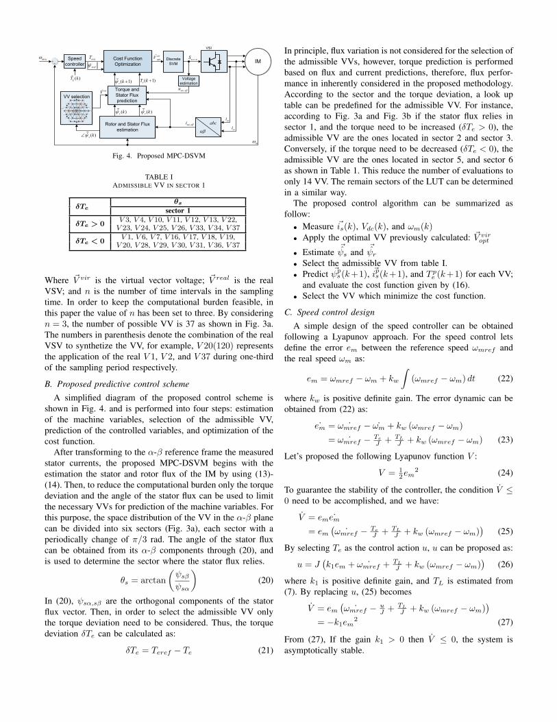
Fig. 4. Proposed MPC-DSVM
TABLE IADMISSIBLE VV IN SECTOR 1
θsδTe sector 1
δTe > 0V 3, V 4, V 10, V 11, V 12, V 13, V 22,V 23, V 24, V 25, V 26, V 33, V 34, V 37
δTe < 0V 1, V 6, V 7, V 16, V 17, V 18, V 19,V 20, V 28, V 29, V 30, V 31, V 36, V 37
Where ~V vir is the virtual vector voltage; ~V real is the realVSV; and n is the number of time intervals in the samplingtime. In order to keep the computational burden feasible, inthis paper the value of n has been set to three. By consideringn = 3, the number of possible VV is 37 as shown in Fig. 3a.The numbers in parenthesis denote the combination of the realVSV to synthetize the VV, for example, V 20(120) representsthe application of the real V 1, V 2, and V 37 during one-thirdof the sampling period respectively.
B. Proposed predictive control scheme
A simplified diagram of the proposed control scheme isshown in Fig. 4. and is performed into four steps: estimationof the machine variables, selection of the admissible VV,prediction of the controlled variables, and optimization of thecost function.
After transforming to the α-β reference frame the measuredstator currents, the proposed MPC-DSVM begins with theestimation the stator and rotor flux of the IM by using (13)-(14). Then, to reduce the computational burden only the torquedeviation and the angle of the stator flux can be used to limitthe necessary VVs for prediction of the machine variables. Forthis purpose, the space distribution of the VV in the α-β planecan be divided into six sectors (Fig. 3a), each sector with aperiodically change of π/3 rad. The angle of the stator fluxcan be obtained from its α-β components through (20), andis used to determine the sector where the stator flux relies.
θs = arctan
(ψsβψsα
)(20)
In (20), ψsα,sβ are the orthogonal components of the statorflux vector. Then, in order to select the admissible VV onlythe torque deviation need to be considered. Thus, the torquedeviation δTe can be calculated as:
δTe = Teref − Te (21)
In principle, flux variation is not considered for the selection ofthe admissible VVs, however, torque prediction is performedbased on flux and current predictions, therefore, flux perfor-mance in inherently considered in the proposed methodology.According to the sector and the torque deviation, a look uptable can be predefined for the admissible VV. For instance,according to Fig. 3a and Fig. 3b if the stator flux relies insector 1, and the torque need to be increased (δTe > 0), theadmissible VV are the ones located in sector 2 and sector 3.Conversely, if the torque need to be decreased (δTe < 0), theadmissible VV are the ones located in sector 5, and sector 6as shown in Table 1. This reduce the number of evaluations toonly 14 VV. The remain sectors of the LUT can be determinedin a similar way.
The proposed control algorithm can be summarized asfollow:
• Measure ~is(k), Vdc(k), and ωm(k)• Apply the optimal VV previously calculated: ~V viropt
• Estimate ~ψs and ~
ψr• Select the admissible VV from table I.• Predict ~ψps (k+1), ~ips(k+1), and T pe (k+1) for each VV;
and evaluate the cost function given by (16).• Select the VV which minimize the cost function.
C. Speed control design
A simple design of the speed controller can be obtainedfollowing a Lyapunov approach. For the speed control letsdefine the error em between the reference speed ωmref andthe real speed ωm as:
em = ωmref − ωm + kw
∫(ωmref − ωm) dt (22)
where kw is positive definite gain. The error dynamic can beobtained from (22) as:
˙em = ˙ωmref − ˙ωm + kw (ωmref − ωm)
= ˙ωmref − TeJ + TL
J + kw (ωmref − ωm) (23)
Let’s proposed the following Lyapunov function V :
V = 12em
2 (24)
To guarantee the stability of the controller, the condition V ≤0 need to be accomplished, and we have:
V = em ˙em
= em(
˙ωmref − TeJ + TL
J + kw (ωmref − ωm))
(25)
By selecting Te as the control action u, u can be proposed as:
u = J(k1em + ˙ωmref +
TLJ + kw (ωmref − ωm)
)(26)
where k1 is positive definite gain, and TL is estimated from(7). By replacing u, (25) becomes
V = em(
˙ωmref − uJ + TL
J + kw (ωmref − ωm))
= −k1em2 (27)
From (27), If the gain k1 > 0 then V ≤ 0, the system isasymptotically stable.

Time (s)
(A)
si(r
ad/s
)m
(N
m)
eTˆ
(Wb)
s
su sv swiii
mrefm
emesTeTLT
Fig. 5. Steady state response of the FS-MPC. From top: stator currents,mechanical speed, electromagnetic torque, stator flux
Time (s)
(A)
si(r
ad/s
)m
(N
m)
eTˆ
(Wb)
s
su sv swiii
mref
m
emesTeTLT
Fig. 6. Steady state response of the MPC-DSVM. From top: stator currents,mechanical speed, electromagnetic torque, stator flux
IV. SIMULATION RESULTS
In order to verify the effectiveness of the proposed control,the system shown in Fig. 4 is implemented in Matlab/Simulinkprogramming environment. The performance of the proposedcontrol is compared with the conventional FS-MPC. Themachine under test is a commercially available IM whoseparameters are listed in table II. For both control schemes,the speed control is carried out based on (26); and the factorλ of the cost function is set to λ = 2. For all control schemesthe IM is magnetized to create the stator flux and reduce initialcurrents, this is done by applying the VSV V2 several timesuntil a 70% of the nominal stator flux is obtained, then, theclose loop control of the IM is performed. In practice, themeasured stator currents are commonly filtered by a low passfilter to avoid noise problems during prediction of the machinevariables.
The performance of the IM in steady state under theconventional FS-MPC and the proposed MPC-DSVM is shown
Time (s)
(A)
si(r
ad/s
)m
(N
m)
eTˆ
(Wb)
s
su sv swiii
mref
m
emesTeTLT
Fig. 7. Transient state response of the MPC-DSVM under speed control.From top: stator currents, mechanical speed, electromagnetic torque, statorflux
TABLE IIPARAMENTERS OF THE IM
415V , 3-Φ, 50 Hz IMParameter value Parameter value
Rs 6.03 Ω ψsnom 1.0 WbRr 6.085 Ω Tenom 7.4 NmLs 0.5192 H p 1Lr 0.5192 H J 0.011787 kgm2
Lm 0.4893 H ωmnom 1415 r/min
in Figs. 5-6. A sampling time of 50 µs for the FS-MPC anda sampling time of 120 µs for the proposed control are used.This sampling time lead to an approximate equal switchingfrequency. In this test the reference speed is set to 150 rad/s.The load torque is equal to 0 Nm during the startup, and at atime of 0.75 s a load torque of 7 Nm is applied. The resultsshow a fast dynamic response of the torque and flux controlduring the startup, which lead to an accurate tracking of thereference speed. It can be noted that under perturbations thespeed remains stable and torque is increased to compensatethe load. It can be seen from Figs. 5-6 that performance ofFS-MPC and MPC-DSVM is similar, however, the proposedMPC-DSVM lead to a higher sampling time, which can beused to perform more complex control algorithms.
The second test is performed to evaluate the transientresponse of the system under MPC-DSVM when a samplingtime of 50 µs is used. The results of the evaluation of MPC-DSVM under speed control is shown in Fig. 7. In this testthe speed is initially set to 150 rad/s and at a time of 1s ischanged to -150 rad/s. For the load torque, a torque of 0 Nmis used during the startup, then load torque is varied from 0to 5 Nm and from 0 to 7 Nm in different instants of time.It can be observed from simulation, that the performance ofthe controller is effective for the speed tracking against torqueload perturbations, and that torque and flux ripples are smallercompared to FS-MPC.

Time (s)
(A)
si(r
ad/s
)m
(N
m)
eTˆ
(Wb)
s
su sv swiii
mref
m
emesTeTLT
Fig. 8. Transient state response of the MPC-DSVM proposed in [13]. Fromtop: stator currents, mechanical speed, electromagnetic torque, stator flux
Finally, a comparison with the method proposed in [13]is carried out. The same parameters used for the transientstate evaluation in previous test are used. It can be seem fromFigs. 7-8, that similar results are obtained from the proposedmethod and the one presented in [13], therefore, a quantitativeevaluation of the torque and flux ripple is performed based onthe flux and torque deviation from the reference values, hence,the standard deviation is used and expressed as percentage.Under Ts = 50µs, this test results in a torque ripple of 3.74%for the proposed method, and a torque ripple of 3.70% ofthe the method presented in [13]. On the other hand, for theproposed method the flux ripple is equal to 0.93%, and for themethod presented in [13] is equal to 1.05%.
The results obtained demonstrate the effectiveness of theproposed control scheme. The proposed MPC-DSVM presentsa similar performance of FS-MPC but with a significant highersampling time. In comparison with [13], the proposed methodresults in a similar torque performance, but a slightly betterflux performance. Moreover, while [13] uses flux and torquedeviation for the selection of the admissible VV, the proposedmethod only uses torque deviation, and from 37 VV only 14VV are required for evaluation.
V. CONCLUSIONS
In this paper a simplified approach for the MPC-DSVMof an IM drive is proposed. By using the torque deviationand the sector where stator flux vector relies, a simplificationin the number of VVs used to predict the behavior of themachine variables is performed, therefore, a reduction of thecomputational burden is aimed to be obtained. Furthermore, asimple speed control design is proposed to improve robustnessof the system. From the simulation results, good performanceunder steady and transient state is obtained, and the response isnot significantly affected by the proposed simplification of theadmissible VV selection. It has been shown that the proposedspeed control lead to fast torque dynamic. The results motivate
the implementation of the proposed control scheme. This issuewill be investigated in the future.
REFERENCES
[1] Bose, B. K. Modern power electronics and AC drives. Upper SaddleRiver, NJ: Prentice hall, 2002.
[2] K. Matsuse and D. Matsuhashi, “New technical trends on adjustablespeed AC motor drives,” in Chinese Journal of Electrical Engineering,vol. 3, no. 1, pp. 1-9, 2017.
[3] R. W. De Doncker, “Modern Electrical Drives: Design and FutureTrends,” 2006 CES/IEEE 5th International Power Electronics and Mo-tion Control Conference, Shanghai, pp. 1-8, 2006.
[4] I. Takahashi and T. Noguchi, “A New Quick-Response and High-Efficiency Control Strategy of an Induction Motor,” in IEEE Transac-tions on Industry Applications, vol. IA-22, no. 5, pp. 820-827, Sept.1986.
[5] R. Gabriel, W. Leonhard and C. J. Nordby, “Field-Oriented Control ofa Standard AC Motor Using Microprocessors,” in IEEE Transactions onIndustry Applications, vol. IA-16, no. 2, pp. 186-192, March 1980.
[6] Y. Zhang, B. Xia, H. Yang and J. Rodriguez, “Overview of modelpredictive control for induction motor drives,” in Chinese Journal ofElectrical Engineering, vol. 2, no. 1, pp. 62-76, June 2016.
[7] Y. Zhang, H. Yang and B. Xia, “Model-Predictive Control of InductionMotor Drives: Torque Control Versus Flux Control,” in IEEE Transac-tions on Industry Applications, vol. 52, no. 5, pp. 4050-4060, Sept.-Oct.2016.
[8] S. Kouro, P. Cortes, R. Vargas, U. Ammann and J. Rodriguez, “ModelPredictive Control—A Simple and Powerful Method to Control PowerConverters,” in IEEE Transactions on Industrial Electronics, vol. 56, no.6, pp. 1826-1838, June 2009.
[9] O. Sandre-Hernandez, J. d. J. Rangel-Magdaleno and R. Morales-Caporal, “Modified model predictive torque control for a PMSM-drivewith torque ripple minimisation,” in IET Power Electronics, vol. 12, no.5, pp. 1033-1042, Jan 2019.
[10] Y. Wang et al., “Deadbeat Model-Predictive Torque Control With Dis-crete Space-Vector Modulation for PMSM Drives,” in IEEE Transactionson Industrial Electronics, vol. 64, no. 5, pp. 3537-3547, May 2017.
[11] P. Karamanakos, P. Stolze, R. M. Kennel, S. Manias and H. duToit Mouton, “Variable Switching Point Predictive Torque Control ofInduction Machines,” in IEEE Journal of Emerging and Selected Topicsin Power Electronics, vol. 2, no. 2, pp. 285-295, June 2014.
[12] D. Casadei, G. Serra and K. Tani, “Implementation of a direct controlalgorithm for induction motors based on discrete space vector modula-tion,” in IEEE Transactions on Power Electronics, vol. 15, no. 4, pp.769-777, July 2000.
[13] M. Amiri, J. Milimonfared and D. A. Khaburi, “Predictive TorqueControl Implementation for Induction Motors Based on Discrete SpaceVector Modulation,” in IEEE Transactions on Industrial Electronics, vol.65, no. 9, pp. 6881-6889, Sept. 2018.
[14] S. Vazquez et al., “Model Predictive Control with constant switchingfrequency using a Discrete Space Vector Modulation with virtual statevectors,” 2009 IEEE International Conference on Industrial Technology,Gippsland, pp. 1-6, VIC, 2009.
[15] M. Habibullah, D. Dah-Chuan Lu, D. Xiao and M. F. Rahman, “Acomputationally efficient FS-PTC for IM with minimum voltage vec-tors,” 2015 IEEE 11th International Conference on Power Electronicsand Drive Systems, pp. 992-997, Sydney, NSW, 2015.
[16] P. Karamanakos, E. Liegmann, T. Geyer and R. Kennel, “ModelPredictive Control of Power Electronic Systems: Methods, Results,and Challenges,” in IEEE Open Journal of Industry Applications, doi:10.1109/OJIA.2020.3020184.
[17] H. Miranda, P. Cortes, J. I. Yuz and J. Rodriguez, “Predictive TorqueControl of Induction Machines Based on State-Space Models,” in IEEETransactions on Industrial Electronics, vol. 56, no. 6, pp. 1916-1924,June 2009, doi: 10.1109/TIE.2009.2014904.
[18] J. Holtz, “The dynamic representation of AC drive systems by complexsignal flow graphs,” Proceedings of 1994 IEEE International Symposiumon Industrial Electronics (ISIE’94), pp. 1-6, Santiago, Chile, 1994.
[19] P. Karamanakos, T. Geyer and R. Kennel, “On the Choice of Norm inFinite Control Set Model Predictive Control,” in IEEE Transactions onPower Electronics, vol. 33, no. 8, pp. 7105-7117, Aug. 2018.