Model predictive control of discrete-time hybrid systems

with discrete inputs ∗

B. Potocnik, G. Music and B. Zupancic

Faculty of Electrical Engineering, University of Ljubljana

Trzaska 25, SI-1000 Ljubljana, Slovenia

Abstract

This paper proposes and discusses a model predictive control approach

to hybrid systems with discrete inputs only. The algorithm, which takes

into account a model of a hybrid system, described as an MLD (mixed

logical dynamical) system, is based on a performance-driven reachability

analysis. The algorithm abstracts the behavior of the hybrid system

by building a “tree of evolution”. The nodes of the tree represent the

reachable states of a process, and the branches connect two nodes if a

transition exists between the corresponding states. A cost-function value

is associated with each node, and based on this value the exploration of

the tree is driven. As soon as the exploration of the tree is finished,

the corresponding input is applied to the system and the procedure is

repeated.

I. INTRODUCTION

Hybrid systems are dynamic systems that involve the interaction of continuous dynamics

(modeled as differential or difference equations) and discrete dynamics (modeled by finite-

state machines). Hybrid systems have been the topic of intense research activity in recent

years, primarily because of their importance in applications [1]. Hybrid models are important

for a number of problems in system analysis, for example, the computation of trajectories,

∗ISA Transactions, 2005, Vol. 44 (2), pp. 199-211.

1

control, stability, and safety analysis.

Several control approaches were proposed in the literature. However, optimal control

approaches for hybrid systems are the most promising ones at the moment, and have been

thoroughly investigated in recent years [12,17]. Many results can be found in the control-

engineering literature. The optimal control of hybrid systems in manufacturing is addressed

in [1,13,16], where the authors combine time-driven and event-driven methodologies to solve

optimal control problems. An algorithm to optimize the switching sequences for a class

of switched linear problems is presented in [20], where the algorithm searches for solutions

that are arbitrarily close to the optimal ones. A similar problem is addressed in [3], where

the potential for numerical optimization procedures to make optimal sequencing decisions

in hybrid dynamic systems is explored. A computational approach based on ideas from dy-

namic programming and convex optimization is presented in [17]. Piecewise linear quadratic

optimal control is addressed in [23], where the use of piecewise quadratic cost functions is

extended from a stability analysis of piecewise linear systems. Optimal control based on

a reachability analysis, and where the inputs of the system are continuous, is addressed

in [6]. A model predictive control technique is presented in [7,5]; this is able to stabilize

the MLD system on desired reference trajectories, and online optimization procedures are

solved through mixed integer quadratic programming (MIQP). Multi-parametric approaches

are thoroughly investigated in [10,11,8,2], where both optimal and model predictive control

approaches are discussed. The latter, in particular, has been successfully applied to many

real problems [21].

In this paper we study and discuss the solution to a model predictive control for linear

discrete-time hybrid systems with discrete inputs only, where the system is described as a

mixed logical dynamical (MLD) system [7]. Many of the control approaches are limited to

discrete-time hybrid systems because many complex mathematical issues are removed. In

many applications the command variables are intrinsically discrete, either because such a

system design is simpler or for other technological reasons. A car with an automatic gear

transmission system is one example where the control system influences the car dynamics

2

only through discrete inputs (gears).

The existing MIQP (MILP) based solutions can also be applied to systems with discrete

inputs, but only in cases with a small number of discrete inputs and a small number of

auxiliary internal system variables (δ and z variables in MLD terminology - see Section

II). The reasons are in the computational complexity of the optimization approach. The

optimization problem is solved in the extended (x, u, z, δ) space with equality constraints,

which increase the size of the problem dramatically [2]. An new approach is proposed in

this paper, which is more efficient than MIQP (MILP) approaches and also more general in

terms of the allowable cost function.

The paper is organized as follows. In Sec. II we address the mixed logical dynamical and

piecewise affine modeling frameworks, as the model predictive approaches based on these

two models will be discussed in the paper. The problems of model predictive control of

hybrid systems with discrete inputs and the proposed solution are addressed in Sec. III.

The proposed algorithm, applied to the model of a motorboat, is discussed in Sec. IV. The

conclusions are given in Sec. V.

II. MIXED LOGICAL DYNAMICAL AND PIECEWISE AFFINE SYSTEMS

In this section mixed logical dynamical systems and piecewise affine systems defined in

discrete time are presented. The model predictive approaches that will be discussed in the

following are based on these two modeling formalisms.

A. Mixed logical dynamical (MLD) systems

Hybrid systems are a combination of logic, finite-state machines, linear discrete-time dy-

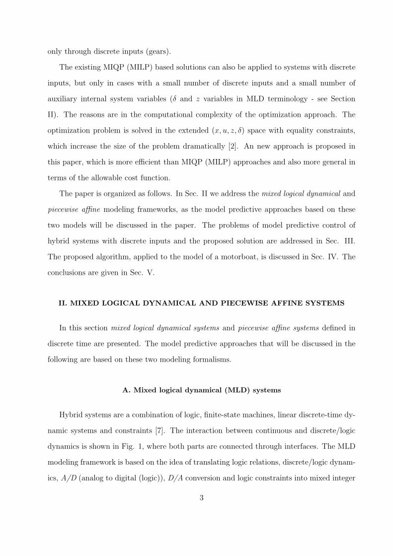
namic systems and constraints [7]. The interaction between continuous and discrete/logic

dynamics is shown in Fig. 1, where both parts are connected through interfaces. The MLD

modeling framework is based on the idea of translating logic relations, discrete/logic dynam-

ics, A/D (analog to digital (logic)), D/A conversion and logic constraints into mixed integer

3

discrete/logicdynamics

continuousdynamics inputs u

states x

symbols di symbols do

A/D D/Ainterface

outputs y

FIG. 1. Hybrid control system – discrete and continuous dynamics interact through interfaces

linear inequalities. These inequalities are combined with the continuous dynamical part,

which is described by linear difference equations. The resulting MLD system is described

by the following relations:

x(k+1)=Ax(k)+B1u(k)+B2δ(k)+B3z(k) (1a)

y(k)=Cx(k)+D1u(k)+D2δ(k)+D3z(k) (1b)

E2δ(k)+E3z(k)≤ E1u(k)+E4x(k)+E5, (1c)

where x(k) ∈ Rnc ×0, 1nb is a vector of continuous and logic states, u(k) ∈ R

mc ×0, 1mb

are the inputs, y(k) ∈ Rpc × 0, 1pb are the outputs and δ ∈ 0, 1rb and z ∈ R

rc are

the logic and continuous auxiliary variables, respectively. The inequalities (Eq. 1c) can also

include physical constraints over continuous variables (states and inputs). Given the current

state x(k) and the input u(k), the time evolution of (1) is determined by solving δ(k) and

z(k) from (1c), and then updating x(k + 1) and y(k) from (1a, 1b). The MLD system (1)

is assumed to be well posed if for a given state x(k) and a given input u(k) the inequalities

(1c) have a unique solution for δ(k) and z(k). Because they are so extensive, the details

of the translation techniques from logic relations, discrete/logic dynamics, A/D (analog to

digital (logic)), D/A conversion and logic constraints into mixed integer linear inequalities,

are not given here. For a more detailed description of MLD form and translation techniques

the reader is referred to [7].

4

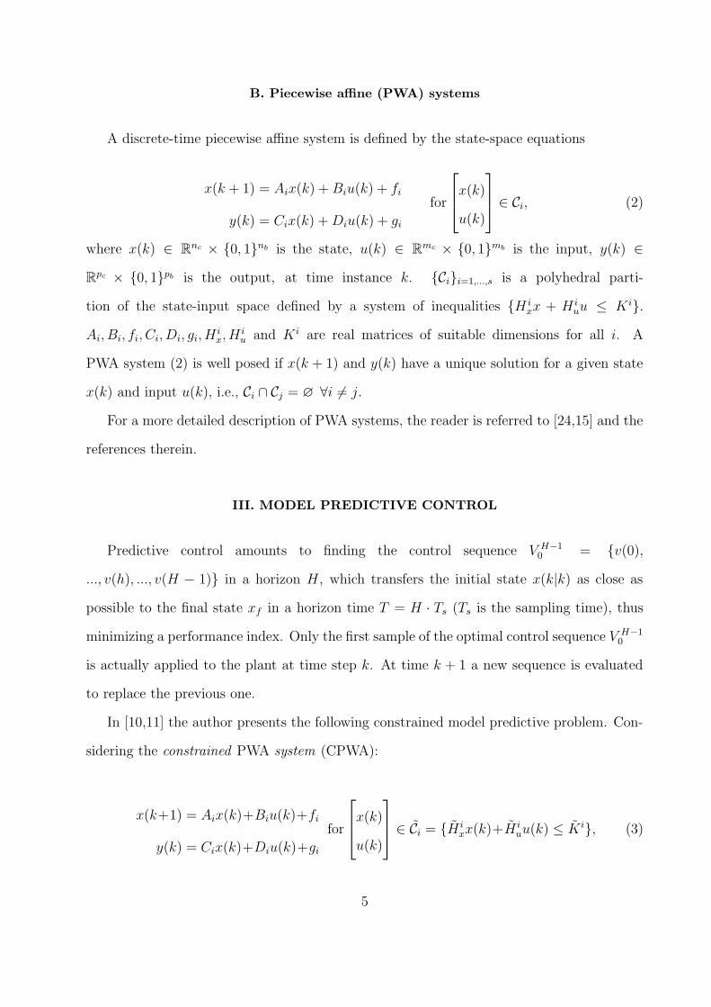
B. Piecewise affine (PWA) systems

A discrete-time piecewise affine system is defined by the state-space equations

x(k + 1) = Aix(k) + Biu(k) + fi

y(k) = Cix(k) + Diu(k) + gi

for

x(k)

u(k)

∈ Ci, (2)

where x(k) ∈ Rnc × 0, 1nb is the state, u(k) ∈ R

mc × 0, 1mb is the input, y(k) ∈

Rpc × 0, 1pb is the output, at time instance k. Cii=1,...,s is a polyhedral parti-

tion of the state-input space defined by a system of inequalities H ixx + H i

uu ≤ K i.

Ai, Bi, fi, Ci, Di, gi, Hix, H

iu and K i are real matrices of suitable dimensions for all i. A

PWA system (2) is well posed if x(k + 1) and y(k) have a unique solution for a given state

x(k) and input u(k), i.e., Ci ∩ Cj = ∅ ∀i 6= j.

For a more detailed description of PWA systems, the reader is referred to [24,15] and the

references therein.

III. MODEL PREDICTIVE CONTROL

Predictive control amounts to finding the control sequence V H−10 = v(0),

..., v(h), ..., v(H − 1) in a horizon H, which transfers the initial state x(k|k) as close as

possible to the final state xf in a horizon time T = H · Ts (Ts is the sampling time), thus

minimizing a performance index. Only the first sample of the optimal control sequence V H−10

is actually applied to the plant at time step k. At time k + 1 a new sequence is evaluated

to replace the previous one.

In [10,11] the author presents the following constrained model predictive problem. Con-

sidering the constrained PWA system (CPWA):

x(k+1) = Aix(k)+Biu(k)+fi

y(k) = Cix(k)+Diu(k)+gi

for

x(k)

u(k)

∈ Ci = H i

xx(k)+H iuu(k) ≤ Ki, (3)

5

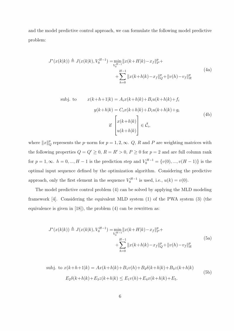
and the model predictive control approach, we can formulate the following model predictive

problem:

J∗(x(k|k)) , J(x(k|k), V H−10 ) =min

V H−1

0

‖x(k+H|k)−xf‖pP +

+H−1∑

h=0

‖x(k+h|k)−xf‖pQ+‖v(h)−vf‖

pR

(4a)

subj. to x(k+h+1|k) = Aix(k+h|k)+Biu(k+h|k)+fi

y(k+h|k) = Cix(k+h|k)+Diu(k+h|k)+gi

if

x(k+h|k)

u(k+h|k)

∈ Ci,

(4b)

where ‖x‖pQ represents the p–norm for p = 1, 2,∞. Q, R and P are weighting matrices with

the following properties Q = Q′ ≥ 0, R = R′ > 0, P ≥ 0 for p = 2 and are full column rank

for p = 1,∞. h = 0, ..., H − 1 is the prediction step and V H−10 = v(0), ..., v(H − 1) is the

optimal input sequence defined by the optimization algorithm. Considering the predictive

approach, only the first element in the sequence V H−10 is used, i.e., u(k) = v(0).

The model predictive control problem (4) can be solved by applying the MLD modeling

framework [4]. Considering the equivalent MLD system (1) of the PWA system (3) (the

equivalence is given in [18]), the problem (4) can be rewritten as:

J∗(x(k|k)) , J(x(k|k), V H−10 ) =min

V H−1

0

‖x(k+H|k)−xf‖pP +

+H−1∑

h=0

‖x(k+h|k)−xf‖pQ+‖v(h)−vf‖

pR

(5a)

subj. to x(k+h+1|k) = Ax(k+h|k)+B1v(h)+B2δ(k+h|k)+B3z(k+h|k)

E2δ(k+h|k)+E3z(k+h|k) ≤ E1v(h)+E4x(k+h|k)+E5.

(5b)

6

A. Multi-parametric approach

In this section the multi-parametric solution to the predictive control problem will be

presented. The aim is to express the approach’s strengths and weaknesses when dealing

with hybrid systems that have discrete inputs.

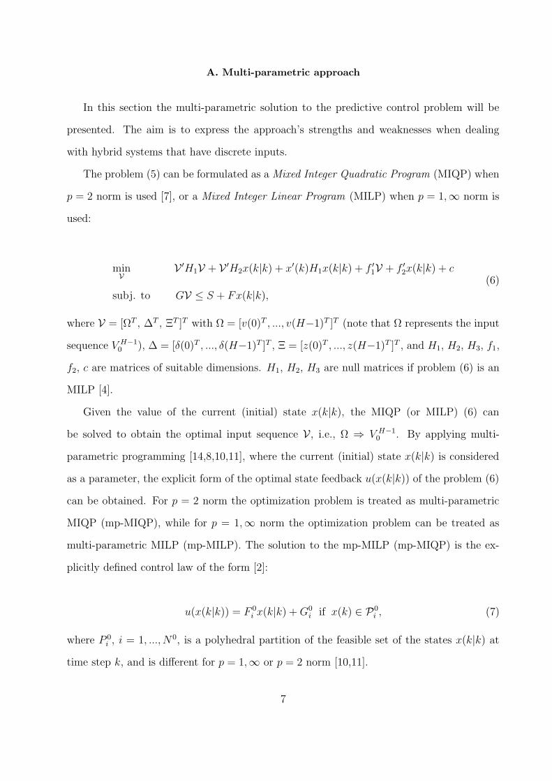
The problem (5) can be formulated as a Mixed Integer Quadratic Program (MIQP) when

p = 2 norm is used [7], or a Mixed Integer Linear Program (MILP) when p = 1,∞ norm is

used:

minV

V ′H1V + V ′H2x(k|k) + x′(k)H1x(k|k) + f ′

1V + f ′

2x(k|k) + c

subj. to GV ≤ S + Fx(k|k),

(6)

where V = [ΩT , ∆T , ΞT ]T with Ω = [v(0)T , ..., v(H−1)T ]T (note that Ω represents the input

sequence V H−10 ), ∆ = [δ(0)T , ..., δ(H−1)T ]T , Ξ = [z(0)T , ..., z(H−1)T ]T , and H1, H2, H3, f1,

f2, c are matrices of suitable dimensions. H1, H2, H3 are null matrices if problem (6) is an

MILP [4].

Given the value of the current (initial) state x(k|k), the MIQP (or MILP) (6) can

be solved to obtain the optimal input sequence V , i.e., Ω ⇒ V H−10 . By applying multi-

parametric programming [14,8,10,11], where the current (initial) state x(k|k) is considered

as a parameter, the explicit form of the optimal state feedback u(x(k|k)) of the problem (6)

can be obtained. For p = 2 norm the optimization problem is treated as multi-parametric

MIQP (mp-MIQP), while for p = 1,∞ norm the optimization problem can be treated as

multi-parametric MILP (mp-MILP). The solution to the mp-MILP (mp-MIQP) is the ex-

plicitly defined control law of the form [2]:

u(x(k|k)) = F 0i x(k|k) + G0

i if x(k) ∈ P0i , (7)

where P 0i , i = 1, ..., N 0, is a polyhedral partition of the feasible set of the states x(k|k) at

time step k, and is different for p = 1,∞ or p = 2 norm [10,11].

7

By looking at the definition of the optimization vector V in (6) and considering the

current state x(k|k) as a parameter, we can see that the mp-MILP (MIQP) approach solves

the problem in extended (x, v(u), δ, z) space, which is numerically very difficult to handle

and increases the size of the problem drastically. The reason is two fold. Firstly, the

complexity of the optimization problem grows exponentially with the number of binary

variables. Therefore, including binary variables δ, which are actually explicitly defined by the

MLD system, state x and input v, into the optimization problem is not efficient. Secondly,

the continuous variables z actually represent equality constraints that were translated into

two sets of inequalities (the consequence of the MLD modeling framework [7]) and which are

also explicitly defined by the MLD system, state x and input v. In [2] an efficient algorithm

for computing the solution for the p = 1,∞ norm case and in [10,11] for p = 2 norm is given.

Both approaches solve the problem in extended (x, v(u)) space and all the problems presented

previously are removed. The algorithms are based on a dynamic programming approach and

mp-LP(QP) solvers. The limitation of the multi-parametric approaches mentioned above is

that they are restricted to hybrid systems where the states x(k) and the inputs u(k) are

defined in x(k) ∈ Rnc and u(k) = v(0) ∈ R

mc , respectively. In spite of these limitations the

approaches were successfully applied to many real problems [21].

When dealing with hybrid systems that also contain binary states or binary inputs, i.e.,

x(k) ∈ Rnc × 0, 1nb and u(k) ∈ R

mc × 0, 1mb , the efficient multi-parametric methods

mentioned above are not applicable and the original mp-MILP (mp-MIQP) complexity re-

mains. Due to the drastic increase in the size of the problem when solving the problem

in extended (x, v(u), δ, z) space, a different approach has to be used. Such an alternative

approach for the case where the hybrid system can be influenced through binary (discrete)

inputs only will be discussed in the following.

8

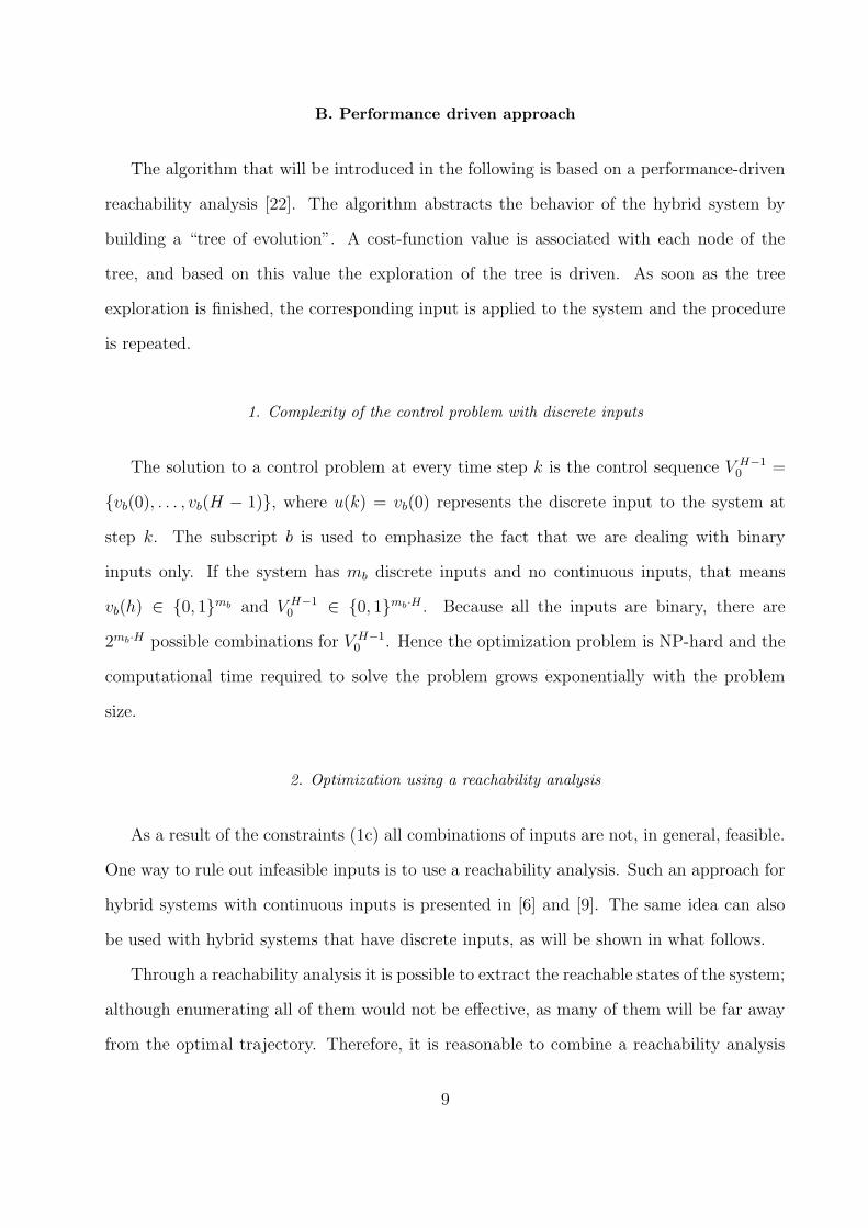
B. Performance driven approach

The algorithm that will be introduced in the following is based on a performance-driven

reachability analysis [22]. The algorithm abstracts the behavior of the hybrid system by

building a “tree of evolution”. A cost-function value is associated with each node of the

tree, and based on this value the exploration of the tree is driven. As soon as the tree

exploration is finished, the corresponding input is applied to the system and the procedure

is repeated.

1. Complexity of the control problem with discrete inputs

The solution to a control problem at every time step k is the control sequence V H−10 =

vb(0), . . . , vb(H − 1), where u(k) = vb(0) represents the discrete input to the system at

step k. The subscript b is used to emphasize the fact that we are dealing with binary

inputs only. If the system has mb discrete inputs and no continuous inputs, that means

vb(h) ∈ 0, 1mb and V H−10 ∈ 0, 1mb·H . Because all the inputs are binary, there are

2mb·H possible combinations for V H−10 . Hence the optimization problem is NP-hard and the

computational time required to solve the problem grows exponentially with the problem

size.

2. Optimization using a reachability analysis

As a result of the constraints (1c) all combinations of inputs are not, in general, feasible.

One way to rule out infeasible inputs is to use a reachability analysis. Such an approach for

hybrid systems with continuous inputs is presented in [6] and [9]. The same idea can also

be used with hybrid systems that have discrete inputs, as will be shown in what follows.

Through a reachability analysis it is possible to extract the reachable states of the system;

although enumerating all of them would not be effective, as many of them will be far away

from the optimal trajectory. Therefore, it is reasonable to combine a reachability analysis

9

with procedures that can detect reachable states not leading to the optimal solution and

remove them from the exploration procedure. The whole procedure is a kind of branch and

bound strategy. The procedure involves the generation of a tree of evolution, as will be

described in the following.

3. Reachability analysis

Let x(k + h|k) be the state at step k + h (h = 0, ..., H − 1). The reachability analysis

computes all the possible states, xi(k+h+1|k), that are reachable in the next time step. If the

system has mb discrete inputs, then 2mb possible next states may exist. However, because of

the constraints (1c), only a smaller number of states can actually be reached. The reachable

states can be computed using the algorithm for reach-set computation described in [9].

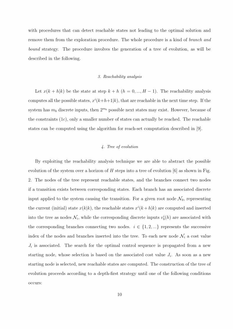
4. Tree of evolution

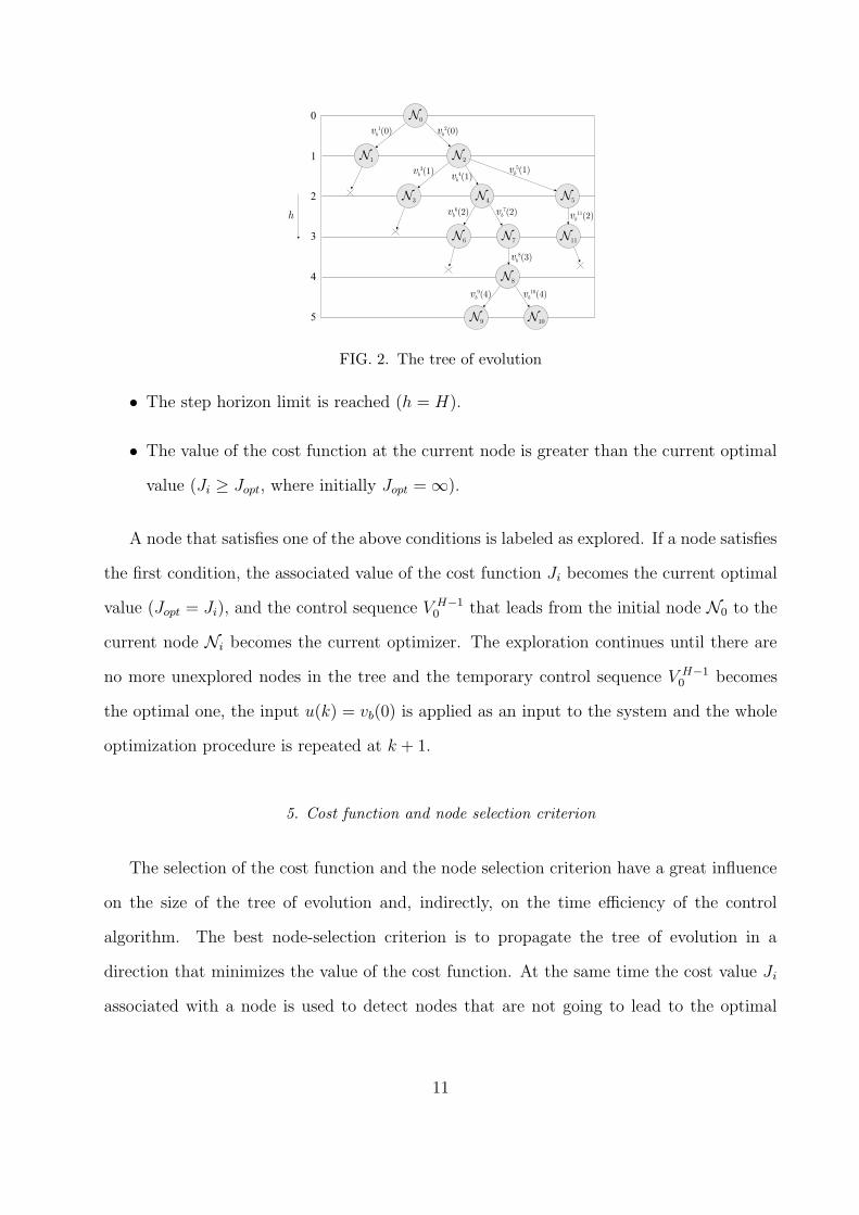
By exploiting the reachability analysis technique we are able to abstract the possible

evolution of the system over a horizon of H steps into a tree of evolution [6] as shown in Fig.

2. The nodes of the tree represent reachable states, and the branches connect two nodes

if a transition exists between corresponding states. Each branch has an associated discrete

input applied to the system causing the transition. For a given root node N0, representing

the current (initial) state x(k|k), the reachable states xi(k +h|k) are computed and inserted

into the tree as nodes Ni, while the corresponding discrete inputs vib(h) are associated with

the corresponding branches connecting two nodes. i ∈ 1, 2, ... represents the successive

index of the nodes and branches inserted into the tree. To each new node Ni a cost value

Ji is associated. The search for the optimal control sequence is propagated from a new

starting node, whose selection is based on the associated cost value Ji. As soon as a new

starting node is selected, new reachable states are computed. The construction of the tree of

evolution proceeds according to a depth-first strategy until one of the following conditions

occurs:

10

N0

N1 N2

N4 N5

N11N7N6

N8

N9 N10

N3

0

1

2

3

4

5

h

vb

1(0) vb

2(0)

vb

3(1)v

b

4(1)v

b

5(1)

vb

6(2) vb

7(2) vb

11(2)

vb

8(3)

vb

9(4) vb

10(4)

FIG. 2. The tree of evolution

• The step horizon limit is reached (h = H).

• The value of the cost function at the current node is greater than the current optimal

value (Ji ≥ Jopt, where initially Jopt = ∞).

A node that satisfies one of the above conditions is labeled as explored. If a node satisfies

the first condition, the associated value of the cost function Ji becomes the current optimal

value (Jopt = Ji), and the control sequence V H−10 that leads from the initial node N0 to the

current node Ni becomes the current optimizer. The exploration continues until there are

no more unexplored nodes in the tree and the temporary control sequence V H−10 becomes

the optimal one, the input u(k) = vb(0) is applied as an input to the system and the whole

optimization procedure is repeated at k + 1.

5. Cost function and node selection criterion

The selection of the cost function and the node selection criterion have a great influence

on the size of the tree of evolution and, indirectly, on the time efficiency of the control

algorithm. The best node-selection criterion is to propagate the tree of evolution in a

direction that minimizes the value of the cost function. At the same time the cost value Ji

associated with a node is used to detect nodes that are not going to lead to the optimal

11

solution. To achieve that, the cost function must have certain properties that we describe

below.

In the case of a classical optimal control problem we typically choose a cost function of

the form:

J(x(k|k), V H−10 ) = ‖x(k+H|k)−xf‖

pP +

H−1∑

h=0

‖x(k+h|k)−xf‖pQ+‖vb(h)−vf‖

pR (8)

where ‖x‖pQ represents the p–norm for p = 1, 2,∞, and where Q, R and P are weighting

matrices with the same properties as in (4a).

For a node Vi inserted into the tree of evolution at the prediction step h < H the associated

cost value (based on (8)) is

Ji(x(k|k), V h−10 , h) =

h∑

j=0

‖x(k+j|k)−xf‖pQ+

h−1∑

j=0

‖vb(j)−vf‖pR. (9)

It is reasonable to detect the nodes Ni that do not lead to the optimal solution at the step

instance h < H (H is horizon) by comparing Ji(h) to Jopt. When the cost value becomes

greater than the current optimal one (Ji ≥ Jopt) we want to ensure that by continuing the

exploration no better solution than the current one can be found. To achieve this the cost

function (9) has to be monotonically increasing with the prediction step. The cost function

(8), (9) fulfils the mentioned condition for p = 1, 2,∞ norm, i.e.,

Ji(x(k|k), V h0 , h + 1) − Ji(x(k|k), V h−1

0 , h) = (10a)

=h+1∑

j=0

‖x(k+j|k)−xf‖pQ+

h∑

j=0

‖vb(j)−vf‖pR −

h∑

j=0

‖x(k+j|k)−xf‖pQ−

h−1∑

j=0

‖vb(j)−vf‖pR =

(10b)

= ‖x(k+h+1|k)−xf‖pQ + ‖vb(h)−vf‖

pR ≥ 0 for h = 1, ..., H − 2. (10c)

and at the horizon, the corresponding difference is ‖x(k+H|k)−xf‖pP +‖vb(H−1)−vf‖

pR ≥ 0.

In the case of a time optimal control problem we must choose a different cost function.

This may be of the form:

Ji(x(k|k), V h−10 , h) = f

(

x(k|k), V h−10

)

+ g(h), h = 1, ..., H, (11)

12

where f(

x(k|k), V h−10

)

is a rewarding function (the “quality” of the control) with the fol-

lowing property

f(

x(k|k), V h+10

)

− f(

x(k|k), V h0

)

≤ 0, (12)

while g(h) is a penalty function (elapsed time) with the following property

g(h + 1) − g(h) > 0. (13)

To maintain the requirement for the cost function (11) to be monotonically increasing with

the prediction step we must choose such a cost function (f(·) and g(·)) that

Ji(x(k|k), V h0 , h + 1) − Ji(x(k + h|k), V h−1

0 , h) ≥ 0 (14a)

i.e.(

f(x(k|k), V h0 ) + g(h + 1)

)

−(

f(x(k|k, V h−10 )) + g(h)

)

≥ 0. (14b)

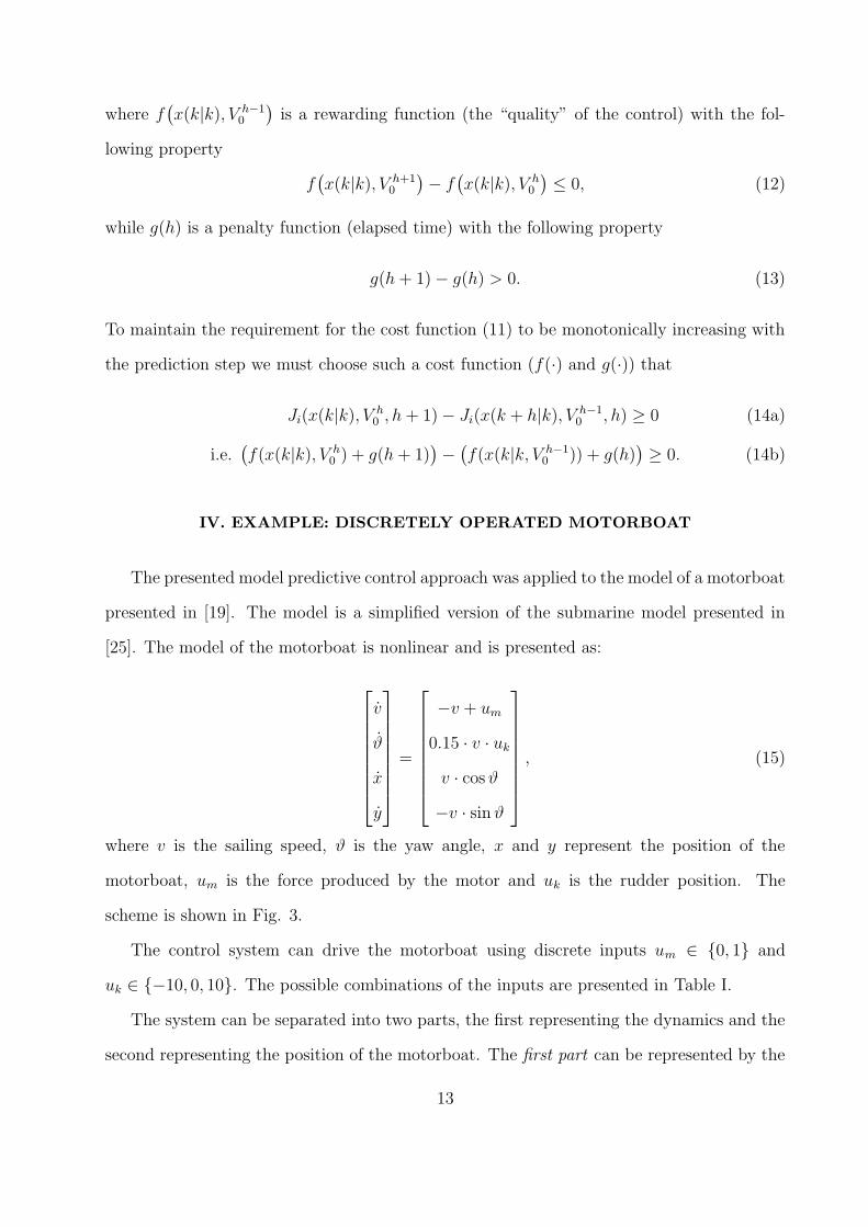
IV. EXAMPLE: DISCRETELY OPERATED MOTORBOAT

The presented model predictive control approach was applied to the model of a motorboat

presented in [19]. The model is a simplified version of the submarine model presented in

[25]. The model of the motorboat is nonlinear and is presented as:

v

ϑ

x

y

=

−v + um

0.15 · v · uk

v · cos ϑ

−v · sin ϑ

, (15)

where v is the sailing speed, ϑ is the yaw angle, x and y represent the position of the

motorboat, um is the force produced by the motor and uk is the rudder position. The

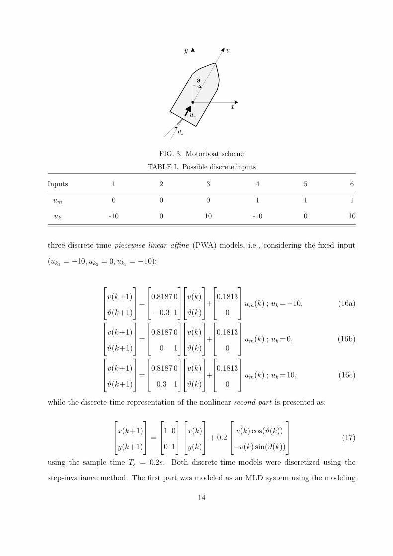
scheme is shown in Fig. 3.

The control system can drive the motorboat using discrete inputs um ∈ 0, 1 and

uk ∈ −10, 0, 10. The possible combinations of the inputs are presented in Table I.

The system can be separated into two parts, the first representing the dynamics and the

second representing the position of the motorboat. The first part can be represented by the

13

y

x

v

um

uk

FIG. 3. Motorboat scheme

TABLE I. Possible discrete inputs

Inputs 1 2 3 4 5 6

um 0 0 0 1 1 1

uk -10 0 10 -10 0 10

three discrete-time piecewise linear affine (PWA) models, i.e., considering the fixed input

(uk1= −10, uk2

= 0, uk3= −10):

v(k+1)

ϑ(k+1)

=

0.8187 0

−0.3 1

v(k)

ϑ(k)

+

0.1813

0

um(k) ; uk =−10, (16a)

v(k+1)

ϑ(k+1)

=

0.8187 0

0 1

v(k)

ϑ(k)

+

0.1813

0

um(k) ; uk =0, (16b)

v(k+1)

ϑ(k+1)

=

0.8187 0

0.3 1

v(k)

ϑ(k)

+

0.1813

0

um(k) ; uk =10, (16c)

while the discrete-time representation of the nonlinear second part is presented as:

x(k+1)

y(k+1)

=

1 0

0 1

x(k)

y(k)

+ 0.2

v(k) cos(ϑ(k))

−v(k) sin(ϑ(k))

(17)

using the sample time Ts = 0.2s. Both discrete-time models were discretized using the

step-invariance method. The first part was modeled as an MLD system using the modeling

14

language HYSDEL (see Appendix). The HYSDEL compiler [26] returned the following

MLD system:

v(k+1)

ϑ(k+1)

=

1 0 0 0

0 1 1 1

z(k) (18a)

1.8187 0 0 01 0 0 01.4562 0 0 01 0 0 01.4562 0 0 01 0 0 01.81871 0 0 0

0 1 0 00 1 0 00 1 0 00 1 0 00 0 1 00 0 1 0

( )0 0 1 00 0 1 00 0 0 10 0 0 10 0 0 10 0 0 10 0 0 00 0 0 00 0 0 00 0 0 0

z k

0.8187 00.8187 00.8187 0

0 0 0 00 10 0 00 10.6 0 00 10.6 0 00 10 0 00 0 10 00 0 10 0

( )0 0 10 00 0 10 00 0 0 100 0 0 10.60 0 0 10.60 0 0 100 1 1 10 1 1 00 1 0 10 0 1 1

u k +

1.63751.6375

00.8187 0100.3 110.60.3 100 000 0100 1100 1

( ) 00 000 0

10.60.3 1100.3 100 000 010 010 0

0 0 10 0 1

x k +

(18b)

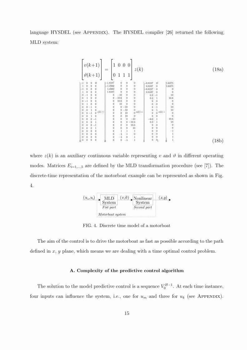
where z(k) is an auxiliary continuous variable representing v and ϑ in different operating

modes. Matrices Ei=1,...,5 are defined by the MLD transformation procedure (see [7]). The

discrete-time representation of the motorboat example can be represented as shown in Fig.

4.

MLD( , )um uk (v,J) (x y, )

Fist part Second part

Motorboat system

SystemNonlinearSystem

FIG. 4. Discrete time model of a motorboat

The aim of the control is to drive the motorboat as fast as possible according to the path

defined in x, y plane, which means we are dealing with a time optimal control problem.

A. Complexity of the predictive control algorithm

The solution to the model predictive control is a sequence V H−10 . At each time instance,

four inputs can influence the system, i.e., one for um and three for uk (see Appendix).

15

The horizon applied was set to H = 3. Considering the number of discrete inputs and the

length of the horizon, there exist 24·3=12 = 4096 possible combinations of the input vector

V H−10 ∈ 0, 112. Of course not all input combinations are possible, i.e., considering six

possible inputs (see Table I) and the horizon H = 3, 63 = 216 feasible input combinations

exist, and many of them lead to non-optimal solutions. By increasing the length of the

horizon the quality of the control does not increase significantly. The reason is the limited

range of the values through which the discrete inputs can influence the dynamics of the

system. Therefore, it is reasonable to choose shorter horizons, as the longer ones increase

the complexity of the control problem exponentially without improving the quality of the

control.

B. Cost-function selection

The aim is to drive the motorboat as fast as possible along a given path. Based on the

cost function and the node selection criteria for the time optimal control problem introduced

earlier, we use the following cost function:

Ji = k − K · s(k + h|k) + D1|xr − x(k + h|k)| + D2|yr − y(k + h|k)|, (19)

where h represents the current step, K is a parameter whose properties will be explained

later, s is the sailed path, D1 and D2 are parameters weighting the deviations from the given

path. According to (14) the cost function (19) has to be monotonically increasing

J(

x(k+h+1|k), y(k+h+1|k), h+1)

− J(

x(k+h|k), y(k+h|k), h)

=

=(

h+1−K·s(k+h+1|k)+D1|xr−x(k+h+1|k)|+D2|yr−y(k+h+1|k)|)

−

−(

h − K · s(k+h|k)+D1|xr−x(k+h|k)|+D2|yr−y(k+h|k)|)

≥ 0.

(20)

For the given path, which can be seen in Fig. 6, the parameters D1 and D2 were set to

D1 = 1 and D2 = 0 or D1 = 0 and D2 = 1 depending on the relative position of the

16

motorboat with respect to the given path. This way we forced the motorboat to sail as

close as possible to the given path. Furthermore, the following relation for parameter K is

obtained:

J(x(k+h+1|k), y(k+h+1|k), h+1)−J(x(k+h|k), y(k+h|k), h) =

= 1 − K(

s(k + h + 1|k) − s(k + h|k))

+

+ D1

(

|xr − x(k + h + 1|k)| − |xr − x(k + h|k)|)

≥ 0

K ≤1 + D1

(

|xr − x(k + h + 1|k)| − |xr − x(k + h|k)|)

s(k + h + 1|k) − s(k + h|k)

. (21)

By considering the worst-case scenario and Dx , |xr − x(k + h + 1|k)| − |xr − x(k + h|k)| =

|xr−x(k+h|k)−∆x|−|xr−x(k+h|k)| ⇒ Dx ∈ [−∆x, ∆x], where ∆x = Ts ·max(v cos(ϑ)) =

0.2 · 1 = 0.2, and ∆s , s(k + h + 1|k) − s(k + h|k) = Ts · max(v cos(ϑ)) = 0.2 · 1 = 0.2, the

parameter K is estimated to be:

K ≤1 − 1 · 0.2

0.2= 4. (22)

Regarding the node selection criterion, it is reasonable to chose the node that leads to the

best current optimal solution, i.e., the node with the smallest associated cost-function value

Ji at step h (the influence of step instance h is the same, but the influence of s is greater).

C. Results

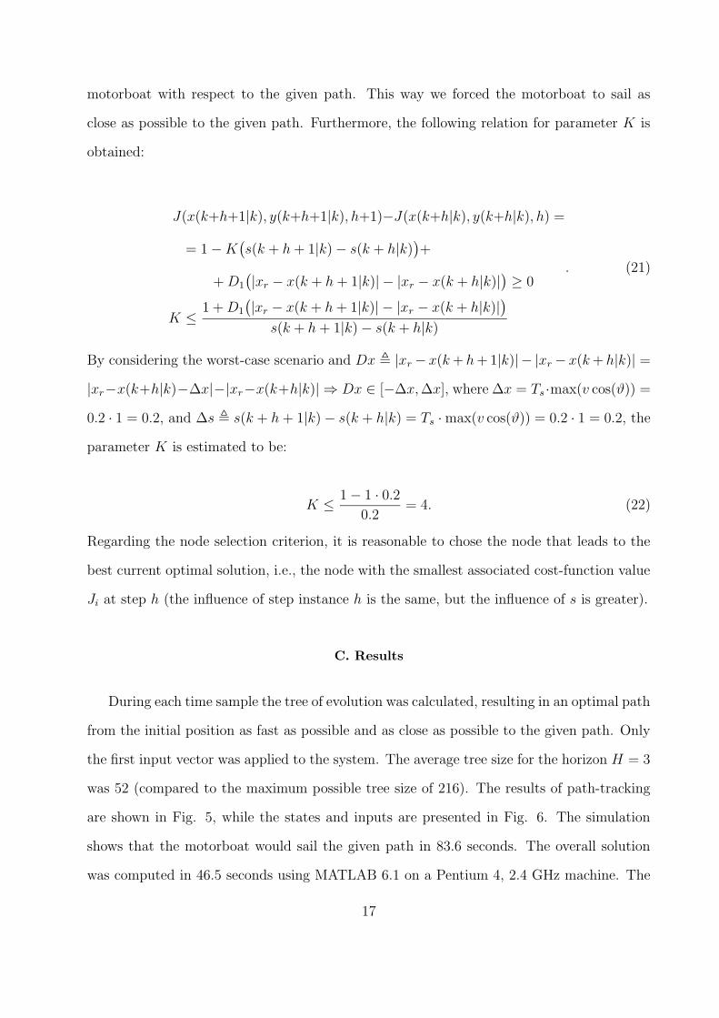
During each time sample the tree of evolution was calculated, resulting in an optimal path

from the initial position as fast as possible and as close as possible to the given path. Only

the first input vector was applied to the system. The average tree size for the horizon H = 3

was 52 (compared to the maximum possible tree size of 216). The results of path-tracking

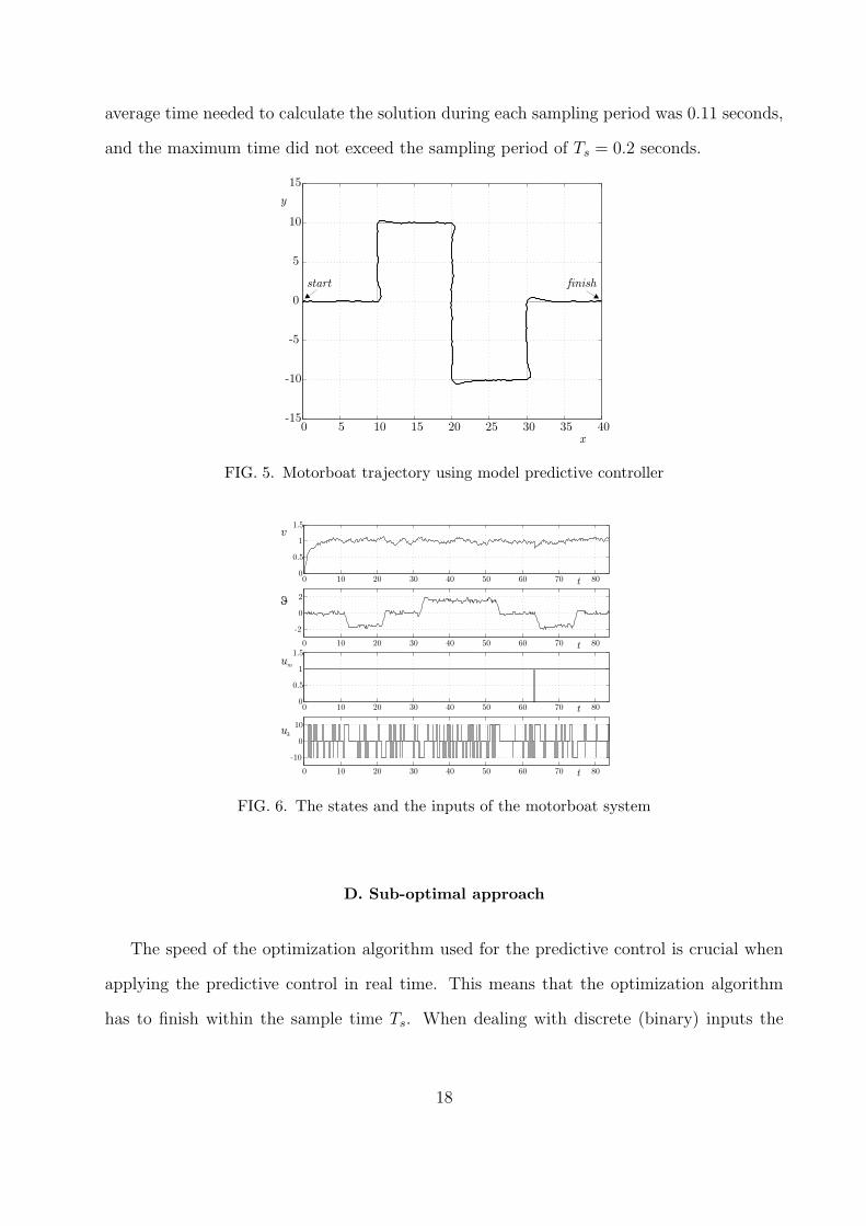
are shown in Fig. 5, while the states and inputs are presented in Fig. 6. The simulation

shows that the motorboat would sail the given path in 83.6 seconds. The overall solution

was computed in 46.5 seconds using MATLAB 6.1 on a Pentium 4, 2.4 GHz machine. The

17

average time needed to calculate the solution during each sampling period was 0.11 seconds,

and the maximum time did not exceed the sampling period of Ts = 0.2 seconds.

0 5 10 15 20 25 30 35 40-15

-10

-5

0

5

10

15

x

y

start finish

FIG. 5. Motorboat trajectory using model predictive controller

0 10 20 30 40 50 60 70 800

0.5

1

1.5

0 10 20 30 40 50 60 70 80

-2

0

2

0 10 20 30 40 50 60 70 800

0.5

1

1.5

0 10 20 30 40 50 60 70 80

-10

0

10

v

J

um

uk

t

t

t

t

FIG. 6. The states and the inputs of the motorboat system

D. Sub-optimal approach

The speed of the optimization algorithm used for the predictive control is crucial when

applying the predictive control in real time. This means that the optimization algorithm

has to finish within the sample time Ts. When dealing with discrete (binary) inputs the

18

problem is even more explicit, as the problem’s complexity grows exponentially with the

number of discrete inputs mb and the horizon H.

The presented approach builds the tree of evolution, proceeding according to a depth-first

strategy. This means that the first sub-optimal solution is obtained as soon as the horizon H

is reached (Jopt = Ji, initially Jopt = ∞). Basically, the algorithm is improving the first sub-

optimal solution until the whole tree is explored and the last sub-optimal solution found is

declared as the optimal one. If the optimization algorithm does not finish the exploration of

the tree within the sample time Ts, the optimization is interrupted and the last sub-optimal

solution is applied to the system. The obtained solution could be the optimal one, but we

cannot guarantee that.

The sub-optimal approach was applied to the motorboat system with the horizon in-

creased to H = 4. Since the number of inputs is mb = 4, then theoretically 24·4 = 65536

possible input sequences V H−10 ∈ 0, 116 exist. In each step only six different inputs can

be applied to the system, and therefore the number of input sequences is reduced to only

64 = 1296.

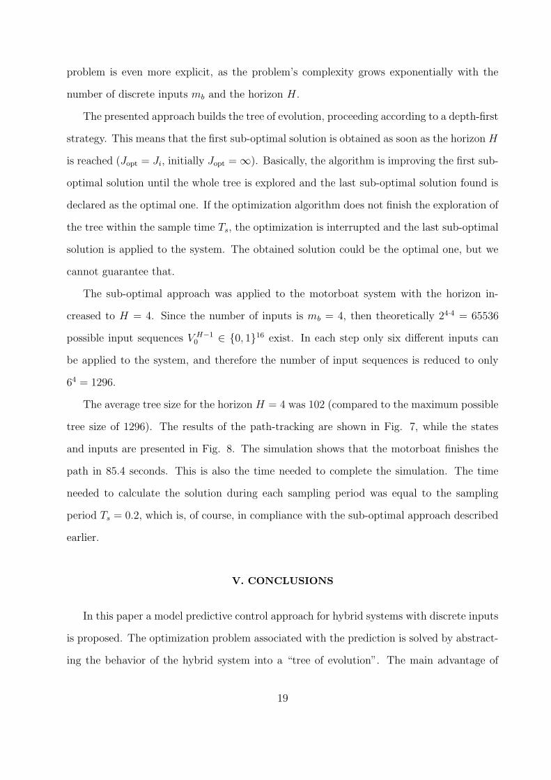
The average tree size for the horizon H = 4 was 102 (compared to the maximum possible

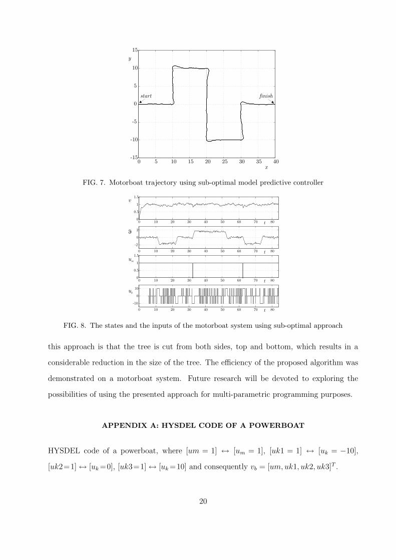
tree size of 1296). The results of the path-tracking are shown in Fig. 7, while the states

and inputs are presented in Fig. 8. The simulation shows that the motorboat finishes the

path in 85.4 seconds. This is also the time needed to complete the simulation. The time

needed to calculate the solution during each sampling period was equal to the sampling

period Ts = 0.2, which is, of course, in compliance with the sub-optimal approach described

earlier.

V. CONCLUSIONS

In this paper a model predictive control approach for hybrid systems with discrete inputs

is proposed. The optimization problem associated with the prediction is solved by abstract-

ing the behavior of the hybrid system into a “tree of evolution”. The main advantage of

19

0 5 10 15 20 25 30 35 40-15

-10

-5

0

5

10

15

x

y

start finish

FIG. 7. Motorboat trajectory using sub-optimal model predictive controller

0 10 20 30 40 50 60 70 800

0.5

1

1.5

0 10 20 30 40 50 60 70 80

-2

0

2

0 10 20 30 40 50 60 70 800

0.5

1

1.5

0 10 20 30 40 50 60 70 80

-10

0

10

v

J

um

uk

t

t

t

t

FIG. 8. The states and the inputs of the motorboat system using sub-optimal approach

this approach is that the tree is cut from both sides, top and bottom, which results in a

considerable reduction in the size of the tree. The efficiency of the proposed algorithm was

demonstrated on a motorboat system. Future research will be devoted to exploring the

possibilities of using the presented approach for multi-parametric programming purposes.

APPENDIX A: HYSDEL CODE OF A POWERBOAT

HYSDEL code of a powerboat, where [um = 1] ↔ [um = 1], [uk1 = 1] ↔ [uk = −10],

[uk2=1] ↔ [uk =0], [uk3=1] ↔ [uk =10] and consequently vb = [um, uk1, uk2, uk3]T .

20

SYSTEM motorboat

INTERFACE

STATE

REAL v [0,2];

REAL th [-10,10];

INPUT

BOOL um,uk1,uk2,uk3;

PARAMETER

REAL v1=0.1813;

REAL v2=0.8187;

IMPLEMENTATION

AUX

REAL vp;

REAL thp1,thp2,thp3;

DA

vp = IF um THEN v2*v+v1 ELSE v2*v ;

thp1=IF uk1 THEN th-0.3*v;

thp2=IF uk2 THEN th+0*v;

thp3=IF uk3 THEN th+0.3*v;

CONTINUOUS

v=vp;

th=thp1+thp2+thp3;

MUST

(uk1&~uk2&~uk3)|(~uk1&uk2&~uk3)|(~uk1&~uk2&uk3);

21

REFERENCES

[1] P.J. Antsaklis, editor. Special issue on hybrid systems: Theory and applications, Pro-

ceedings of the IEEE, volume 88, 2000.

[2] M. Baotic, F.J. Christophersen, and M. Morari. A new algorithm for constrained fi-

nite time optimal control of hybrid systems with a linear performance index. Technical

report, Automatic Control Laboratory, Swiss Federal Institute of Technology (ETH),

Zrich, 2002.

[3] P.I. Barton, J.R. Banga, and S. Galan. Optimization of hybrid discrete/continuous

dynamic systems. Computers and Chemical Engineering, 24:2171–2182, 2000.

[4] A. Bemporad, F. Borrelli, and M. Morari. On the optimal control law for linear discrete

time hybrid systems. In Hybrid Systems: Computation and Control, volume 2289 of

Lecture Notes in Computer Science, pages 105–119. Springer Verlag, 2002.

[5] A. Bemporad, G. Ferrari-Trecate, D. Mignone, M. Morari, and F.D. Torrisi. Model

predictive control - ideas for the next generation. In European Control Conference,

Karlsruhe, Germany, 1999.

[6] A. Bemporad, L. Giovanardi, and F.D. Torrisi. Performance driven reachability analysis

for optimal scheduling and control of hybrid systems. In Proceedings of the 39th IEEE

Conference on Decision and Control, pages 969–974, Sydney, Australia, 2000.

[7] A. Bemporad and M. Morari. Control of systems integrating logic, dynamics, and con-

straints. Automatica, 35(3):407–427, 1999.

[8] A. Bemporad, M. Morari, V. Dua, and E.N. Pistikopoulos. The explicit linear quadratic

regulator for constrained systems. Automatica, 38(1):3–20, 2002.

[9] A. Bemporad, F.D. Torrisi, and M. Morari. Optimization-based verification and stability

characterization of piecewise affine and hybrid systems. In Hybrid Systems: Computation

22

and Control, volume 1790 of Lecture Notes in Computer Science, pages 45–58. Springer

Verlag, 2000.

[10] F. Borrelli. Discrete Time Constrained Optimal Control. PhD thesis, Automatic Control

Laboratory, Swiss Federal Institute of Technology (ETH), Zrich, 2002.

[11] F. Borrelli. Constrained Optimal Control of Linear and Hybrid Systems, volume 290 of

Lecture Notes in Control and Information Sciences. Springer Verlag, 2003.

[12] M.S. Branicky, V.S. Borkar, and S.K. Mitter. A unified framework for hybrid control:

Model and optimal control theory. IEEE Transactions on Automatic Control, 43(1):31–

45, 1998.

[13] C.G. Cassandras, D.L. Pepyne, and Y. Wardi. Optimal control of a class of hybrid

systems. IEEE Transactions on Automatic Control, 46(3):398–415, 2001.

[14] V. Dua, N.A. Bozinis, and E.N. Pistikopoulos. A multiparametric programming ap-

proach for mixed-integer quadratic engineering problems. Computers & Chemical En-

gineering, 26(4–5):715–733, 2002.

[15] G. Ferrari-Trecate, F.A. Cuzzola, D. Mignone, and M. Morari. Analysis of discrete-time

piecewise affine and hybrid systems. Automatica, 38(12):2139–2146, 2002.

[16] K. Gokbayrak and C.G. Cassandras. A hierarchical decomposition method for optimal

control of hybrid systems. In Proceedings of the 38th IEEE Conference on Decision and

Control, pages 1816–1821, Phoenix, Arizona, USA, 1999.

[17] S. Hedlund and A. Rantzer. Optimal control of hybrid systems. In Proceedings of the

38th IEEE Conference on Decision and Control, pages 3972–3976, Phoenix, Arizona,

USA, 1999.

[18] W.P.M.H. Heemels, B. De Schutter, and A. Bemporad. Equivalence of hybrid dynamical

models. Automatica, 37(7):1085–1091, 2001.

23

[19] M. Sikovc. Control of hybrid systems (in Slovene). Master’s thesis, Faculty of Electrical

Engineering, University of Ljubljana, 1998.

[20] B. Lincoln and A. Rantzer. Optimizing linear system switching. In Proceedings of the

40th IEEE Conference on Decision and Control, pages 2063–2068, Orlando, Florida,

USA, 2001.

[21] M. Morari, M. Baotic, and F. Borrelli. Hybrid systems modeling and control. European

Journal of Control, 9(2–3):177–189, 2003.

[22] B. Potocnik, A. Bemporad, F.D. Torrisi, G. Music, and B. Zupancic. Hybrid mod-

elling and optimal control of a Multiproduct Batch Plant. Control Engineering Practice,

12(9):1127-1137, 2004.

[23] A. Rantzer and M. Johansson. Piecewise linear quadratic optimal control. IEEE Trans-

actions on Automatic Control, 45(5):629–637, 2000.

[24] E.D. Sontag. Nonlinear regulation: The piecewise linear approach. IEEE Transactions

on Automatic Control, 26(2):346–358, 1981.

[25] J.A. Stiver, P. J. Antsaklis, and M.D. Lemmon. Hybrid control system design based on

neural invariants. In Proceedings of the 34th IEEE Conference on Decision and Control,

pages 1455–1460, New Orleans, LA, 1995.

[26] F.D. Torrisi and A. Bemporad. HYSDEL – a tool for generating computational hybrid

models. IEEE Transactions on Control Systems Technology – Special Issue on Computer

Automated Multi-Paradigm Modeling, in press, 2002.

24