a dual-discrete model predictive control-based mppt for pv

Aalborg Universitet

A Dual-Discrete Model Predictive Control-based MPPT for PV systems

Lashab, Abderezak; Séra, Dezso; Zapata, Josep Maria Guerrero

Published in:I E E E Transactions on Power Electronics

DOI (link to publication from Publisher):10.1109/TPEL.2019.2892809

Publication date:2019

Document VersionAccepted author manuscript, peer reviewed version

Link to publication from Aalborg University

Citation for published version (APA):Lashab, A., Séra, D., & Zapata, J. M. G. (2019). A Dual-Discrete Model Predictive Control-based MPPT for PVsystems. I E E E Transactions on Power Electronics, 34(10), 9686 - 9697. [8611184].https://doi.org/10.1109/TPEL.2019.2892809

General rightsCopyright and moral rights for the publications made accessible in the public portal are retained by the authors and/or other copyright ownersand it is a condition of accessing publications that users recognise and abide by the legal requirements associated with these rights.

- Users may download and print one copy of any publication from the public portal for the purpose of private study or research. - You may not further distribute the material or use it for any profit-making activity or commercial gain - You may freely distribute the URL identifying the publication in the public portal -

Take down policyIf you believe that this document breaches copyright please contact us at [email protected] providing details, and we will remove access tothe work immediately and investigate your claim.

Downloaded from vbn.aau.dk on: January 30, 2022

https://doi.org/10.1109/TPEL.2019.2892809

https://vbn.aau.dk/en/publications/60b3de0d-6de7-4446-9402-d462fa7b676d

https://doi.org/10.1109/TPEL.2019.2892809

0885-8993 (c) 2018 IEEE. Personal use is permitted, but republication/redistribution requires IEEE permission. See http://www.ieee.org/publications_standards/publications/rights/index.html for more information.

This article has been accepted for publication in a future issue of this journal, but has not been fully edited. Content may change prior to final publication. Citation information: DOI 10.1109/TPEL.2019.2892809, IEEETransactions on Power Electronics

1

Abstract--This paper presents a method that overcomes the

problem of the confusion during fast irradiance change in the classical MPPTs as well as in model predictive control (MPC)-based MPPTs available in the literature. The previously introduced MPC-based MPPTs take into account the model of the converter only, which make them prone to the drift during fast environmental conditions. Therefore, the model of the PV array is also considered in the proposed algorithm, which allows it to be prompt during rapid environmental condition changes. It takes into account multiple previous samples of power, and based on that is able to take the correct tracking decision when the predicted and measured power differ (in case of drift issue). After the tracking decision is taken, it will be sent to a second part of the algorithm as a reference. The second part is used for following the reference provided by the first part, where the pulses are sent directly to the converter, without a modulator or a linear controller. The proposed technique is validated experimentally by using a buck converter, fed by a PV simulator. The tracking efficiency is evaluated according to EN50530 standard in static and dynamic conditions. The experimental results show that the proposed MPC-MPPT is a quick and accurate tracker under very fast changing irradiance, while maintaining high tracking efficiency even under very low irradiance.

Index Terms-- Buck converter, dc-dc power conversion, Drift,

Double cost function, EN50530 standard, Maximum power point tracking, MPC, Photovoltaic systems.

I. INTRODUCTION

HOTOVOLTAIC (PV) electricity production system is one of the most essential renewable energy systems, due to its advantageous features, primarily the clean, free, and

unlimited resource. It is predicted that in 2035, the energy generated by PV systems will increase by almost 20 times, expanding to 846TWh [1].

Under each irradiance/temperature level, the PV array provides different output power vs voltage characteristic P(v). This latter, is nonlinear and in normal conditions has only one peak, indeed it has a shape close to the intersection shape “∩”. The peak of this curve is usually referred to as the maximum power point (MPP). Various algorithms have been proposed in the literature for defining and making the PV module working

The authors are with the Department of Energy Technology, Aalborg

University, 9220 Aalborg, Denmark (e-mail: [email protected]; [email protected]; [email protected]).

under this peak simultaneously [2]. These algorithms are named as maximum power point trackers (MPPT). The classical and the most well-known MPPT is the Perturb and Observe (P&O). In fact, this algorithm is simple and requires only the use of sensors for measuring the PV current and voltage. But, as its name denotes, this algorithm continuously perturbs the voltage (in case of voltage control) by adding/subtracting a fixed voltage increment (ΔV) to/from the PV voltage, which produces some oscillations in the output PV power. Also, its speed convergence is limited, by reason that the choice of the step size is linked to the steady state operation conditions [3], [4]. Incremental Conductance (INC) also is a well-known MPPT [5], [6], and its operational principle is very congruous to that of P&O algorithm. It therefore provides tantamount static and dynamic perfor-mances as P&O according to the investigation reported in [7]. There exist other classical methods, such as fractional open-circuit voltage (FOCV) [8], and fractional short-circuit current (FSCC) [2]. But, these methods do not converge to the true MPP, and they suffer from power loss during the measurement of the fractional variable. The relative merits of these numerous approaches are discussed and investigated in [2].

The fact that the classical MPPTs fail to pursue the MPP under rapidly changing atmospheric conditions, has raised concern of many researchers [9]-[14]. This issue is referred as drift in the literature [9]. For instance, the conventional P&O fails to track the MPP during fast environmental condition changes, because this algorithm and its rules are designed for a static PV curve, and if there is a fast change in the irradiance/temperature, the rules of this algorithm are no longer sufficient. As a scenario, if the result of the condition Ppv(k)-Ppv(k-1)>0 is yes, P&O considers that the operating point is approaching the MPP, and subsequently, the same decision as the previous one will be taken. However, there is another probability P&O is not designed to be aware of, which is, the increase of power caused by the increase of irradiance during one perturbation period is larger than the increase in power induced by the previous perturbation. In this case, the operating point is may be going far away from the MPP. In [9], a condition has been added to P&O by observing the change in current, which provides to P&O the knowledge when the operating point goes to the right side of the MPP. But, the operating point may go to the right or left side of the MPP, that depends upon the last action taken by P&O just prior to the irradiance change. In [10], the change of power resulted by the environmental condition changes is subtracted from the overall resulted PV power, to allow the P&O

A Dual-Discrete Model Predictive Control-Based MPPT for PV Systems

Abderezak Lashab, Student Member, IEEE, Dezso Sera, Senior Member, IEEE, and Josep M. Guerrero, Fellow, IEEE

P



2

discriminate the change in power resulted by incre-menting/decrementing the involved reference from the power caused by the insolation changes. In [11], maximum and minimum boundaries have been set to limit the PV voltage around the estimated MPP. This avoids undesirable excursions of the PV voltage during rapidly changing atmospheric conditions. In [12], multi-sampling (MS) MPPT has been developed, in which a voltage step size is incremented and decremented and incremented (+-+), and based on the behavior of the PV power caused by these actions, the right decision will be set. This approach provides a good dynamics. However, in some cases, under very fast irradiance change, the same action should be set successively in order to track the MPP. In [13], an adaptive algorithm that tunes continuously the size of the increment in P&O has been proposed. Although this technique alleviates the drift, large oscillations are produced during the change in irradiance. Moreover, according to realistic weather changes, if the MPP controller is sufficiently sophisticated to provide right decisions during varying irradiance/temperature, a fixed step size would be adequate even if the atmospheric change is fast [41]-[42]. The combination of FSCC and P&O has been proposed in [14] to detect the change in irradiance. The method starts first with FSCC by estimating the current of the MPP based on the measured short circuit current. Afterwards, the algorithm starts working by using P&O. At each iteration, the PV current is compared with one calculated first with FSCC, if the differ-ence exceeds a certain limit (in case of irradiance change), the algorithm start over. The convergence time is short at the start-up, and the drift issue is mitigated, however, may still some losses since the operation principle is approximation based.

Recently, intelligent controllers such as fuzzy logic controller [15], neural network controller [16], sliding mode [17], and model predictive controller [25], have been used for tracking the MPP to overcome the drawbacks of the classical ones. Both fuzzy logic and neural network controllers are appropriate for applications where the mathematical model of the system or some of its parameters are undefined. Sliding mode offers robustness and takes into consideration the switching nature of the power converter [21]. The main feature of MPC is its estimation of the future conduct of the controlled variable.

The computational cost of MPC, which was important in the past years, has now become a minor issue, since powerful digital microprocessors and FPGAs that can execute complex calculations in a short time were developed. This fact has led to a significant attention to the implementation of MPC in power electronics applications such as dc-dc converters, electric drives, multilevel inverters, and matrix converters [18]-[20]. MPC in power electronics is subdivided into two main categories [21], [22]: continuous control set MPC (CCS-MPC) and finite control set MPC (FCS-MPC). In the first class, the gate drive signals are generated from a modulator, where its input is a continuous predicted variable. The second class exploits the finite number of the switching states of the converter to restrain the error between the controlled variable and its given reference [22].

As reported in the literature, MPC in MPPTs is subdivided into two major classes, CCS-MPC-MPPT [23]-[24] and Discrete-MPC-MPPT, the later itself is subdivided into FCS-

MPC-MPPT [25]-[29] and Digital Observer (DO)-MPC-MPPT [30]-[31].

In FCS-MPC-MPPT, the discrete-time model of the system is used to predict the behavior of the controlled variable up to N horizon length. The switching state that entails a minimized cost function will be selected to be applied during the next sampling time directly to the converter without the necessity of a PI controller or a modulation stage. Among the merits of FCS in power electronics generally are its fast dynamic response and its ability of handling nonlinearities, as well as including multi-variables in the cost function. The references provided to FCS-MPC-MPPT are calculated by using P&O [25] or INC [26]-[29]. In DO-MPC-MPPT, a digital observer is adopted for the prediction of a PV currents conformable to an assumed PV voltages, where the PV voltages are shifted by a predicted step size. In [32], the efficiency of Discrete-MPC-based MPPT has been deeply studied, considering different weather conditions as well as various power converter topologies, and, as it has been reported, when using FCS-MPC-based MPPT; the resulted MPP tracker will have the same shortcomings as the used reference (in that paper P&O is considered). Regarding DO-MPC-MPPT, a better performance during a changing environmental conditions compared to FCS-MPC-MPPT can be obtained, but tracking the MPP under fast environmental condition changes is still a challenge for DO-MPC as well.

Based on the existing body of literature, the drift issue in MPC-MPPTs is still unsolved, which retained the research in this area ongoing. In this paper, a method using model predictive control in both sides, PV and converter is proposed, where the main objective is drift avoidance during fast irradiance change by using MPC.

II. OPERATION PRINCIPLE OF FINITE-CONTROL-SET MPC-BASED MPPT

The dc-dc buck topology used in this paper is illustrated in Fig. 1. Since only one switch is used in the selected topology, the control operation is simpler than other topologies, such as, series capacitor buck converter [33]. A one step ahead is the horizon length used in this paper. The first step of FCS-MPC-MPPT implementation procedure is defining the system equations. By applying Kirchhoff´s voltage and current laws on the electrical circuit in Fig. 1, the model in continuous-time domain of the buck converter for the two states can be found as follows Switch ON

2

Lpv C2 L L

C2L R

diL = v

dtdv

C = i idt

v r i

(1)

Switch OFF

2

Laux C2 aux L L

C2aux L R

diL = v

dtdv

C = i idt

d d r i

d

(2)

such as the four state variables vpv, iL, vC2 and, iR are the PV



3

voltage, the current through the inductor L, the output voltage of the converter, and the current going through the load R, respectively. daux is equal to “1” during the continuous current mode (CCM), whereas during the discontinuous current mode (DCM) and after the switch opens and the current in the inductor gets nulled, it takes the value of “0” [34]. In what follows, it is assumed that the inductor stray resistance rL is equal to zero, and the converter is operating in CCM.

Usually, the discrete-time model of the system is obtained by using Euler´s forward-difference law, which can be expressed as

dx x x

dt

( ) ( )k + 1 kTs

‐ (3)

where Ts is the sampling time. The substitution of (3) into buck converter’s Switch ON equations yields to

( ) ( ) ( ) ( )

( ) ( ) ( ) ( )

L pv C2 L

C2 L R C22

v +

i i

Tsi k + 1 k v k i k

LTs

v k + 1 = k + 1 k v kC

(4)

The model of buck converter’s Switch OFF state in discrete-time domain was found similarly as

( ) ( ) ( )

( ) ( ) ( ) ( )

L C2 L

C2 L R C22

v +

i i

Tsi k +1 = k i k

LTs

v k +1 = k +1 k + v kC

(5)

The average value of the current going through the capacitor C2 is zero. Hence, the average current going through the inductor L equals to the average value of the output current. The relationship between the inductor current and input current can be then expressed as follows

( ) ( )pv Li k +1 D i k +1 . (6)

where D is the duty cycle of the gating signal. The predicted PV current can be calculated by substituting

(6) into (4) and (5). Generally, the cost function is calculated by using the predicted variables and their references, where the references are calculated based on P&O or INC algorithm,

0,1 0,1 0,1( ) ( )pv v pvi k +1 i v k +1 v g +I * * (7)

Fig. 1. A simplified configuration of PV system interfaced by a dc-dc buck converter.

Fig. 2. (a) equivalent dc-dc buck converter during Switch ON state, (b) equivalent dc-dc buck converter during Switch OFF state.

Fig. 3. Overview of the proposed approach.

where, λI and λv are the current and voltage weighting factors, respectively. In the cost function, each term is weighted through these weighting factors in order to reach the desired balance between the priorities among the control targets and constraints. Definitely, the larger the weighting factor, the larger priority assigned to the corresponding term. Different approaches are usually used to determine the weighting factors, the most adopted one is based on empirical methods [22]. Despite the fact that in [35] some guidelines for the design of the weighting factors are given, there are still no analytical or mathematical methods to ultimately overcome this issue. The weighting factors design could be complex since in some systems the design done for a specific operating region, is not valid for another one. On that account, intelligent controllers, such as, Artificial Neural Network [36] and Fuzzy Logic [36][37] are being employed to address this issue, where the optimization process is performed online.

After the cost function optimization, the controller has to wait until tk reaches Ts. Where tk is the time from the last application of the gate signals. Thereafter, the switching state corresponding to the evaluated cost function can be applied directly to the converter.

III. PROPOSED MODEL PREDICTIVE CONTROL-BASED MPPT

In the literature, P&O and its alternate implementation, the INC are the ones used for providing the references to FCS-MPC [25]-[29]. But, P&O and INC methods have a poor dynamic performance under rapidly varying environmental conditions, which influence on the MPPT efficiency negatively. Also, the generated power by using these two methods fluctuates in the steady state, causing some losses. The application of FCS with the inclusion of these two main drawbacks of P&O/INC method, will result to an MPPT hampered by them. For this purpose, an improved predictive control algorithm has been designed in this paper, its flowchart is sketched in Fig. 5. The novelty of this work consists of integrating two predictions into a single MPP tracker as depicted in Fig. 3, where: The first prediction is based on the estimation of the

predicted PV voltage/current on the extrapolated PV curve, which will then serve as a reference (blue color in Fig. 3). The prominent role of these predictions is during dynamic weather conditions as will be explained next.

In order to increase the dynamic reference tracking performance during the start-up of the system, and also during load variation, the dynamic behavior of the converter is going to be predicted by introducing FCS-

C1 C2

Li

v

i

vD

S

i

PV R

RLPV

C2PV

rL

C1 C2

Li i iRL

C1 C2

Li iR

R R

PV PVrL

vPV

vPV

v

vC2

rL

C2

(a) (b)

Actual samlpe

Part of the PV curve extraploation (Lagrange)

Two previous samples

Converter model

FCS‐MPC

Predicted PV current/voltage

Converter Gating signal

Apply an opposite action to the on appiled in the

previous sampling time

Does the predicted power at

the previous sampling time equal to the actual

power?

Yes

NoI (k+1)*PV



4

MPC as a second prediction part in the proposed algorithm, which also allows the elimination of the PI controller from the voltage/current regulation loop as well as the modulation stage (red color in Fig. 3).

1) Static weather conditions A. Reference Generation In MPC techniques, the discretized equations of the system

are used for the estimation of the future action of the controlled variable. Concerning the PV array, a high accuracy model of the system is extremely difficult and unpractical to build, because a lot of factors are continuously changing such as the solar irradiance, temperature, and the degradation of the PV modules. For this reason, an algorithm that identifies the model of part of the PV curve at each sampling period by interpolating it based on Lagrange polynomial has been developed in this work (please see Fig. 4). Lagrange polynomial (POl) is interpolated using a data points as follows

........ .( ) 0,1 .. , ..,i iPol x y for i n

And Lagrange polynomial will have the following form 1 2

1 2 1 0( ) ...n nn nPol x a x a x a x a x a

(8) 1 2

0 0 0 0 0

1 21 11 1 1 1

1 20

... ... ... ...

... ... ... ...

....... ....... ..

... 1

.

...

... ... ..

.

.

. 1

... .. 1.

n n nn

n n nn

n n nnn n n n

x x x x a y

a yx x x x

yax x x x

(9)

By substituting (8) in (9), we get a system of set of equations in am coefficients. The matrix on the left is usually referred to as Vandermonde Matrix. There are various proposed algorithms that exploit the scheme of Vandermonde Matrix to compute stable solutions by Gaussian elimination [38], [39]. The interpolated polynomial can be written in terms of the Lagrange polynomials as follows

1 20

0 1 0 2 0

0 21

1 0 1 2 1

0 1 1

0 1

( )( ) ( )( )

( )( ) ( )

( )( )::::::::::::::

:::::::::::::::::::::::::::::::::

:::::::::

( )

( )( ) ( )

( )( ) ( )

( )( )::

n

n

n

n

n

n n

x x x x x xPol x y

x x x x x x

x x x x x xy

x x x x x x

x x x x x x

x x x x

1( ) nn n

yx x

(10)

Fig. 4. Extrapolation of the predicted current based on the predicted PV voltage and the interpolated PV curve.

Fig. 5. Flowchart of the proposed MPC-MPPT.

Lagrange polynomials are generally expressed in Sylvester´s Formula, as the following way

::0 0

( )n

ji

i j n i jj i

x xPol x y

x x

(11)

To interpolate a part of the PV curve that is in the neighborhood of the operating point, a data points constituted of ipv(k-2){vpv(k-2)}, ipv(k-1){vpv(k-1)}, and ipv(k){vpv(k)} are used. Where k-2 denotes to the sampling time before the last one, k-1 denotes to the previous sampling time, and k denotes to the present sampling time. Hence, the following Lagrange polynomial for the PV curve is proposed

22 1 0( ) ( ) ( )pv pv pvv k a i k a i k a (12)

Vandermonde Matrix can be then written as follows

2

2

21

20

( ) ( ) 1 ( )

( ) ( ) 1 ( )

( )( ) ( ) 1

pv pv pv

pv pv pv

pvpv pv

i k - 2 i k - 2 v k - 2a

i k - 1 i k - 1 a v k - 1

a v ki k i k

(13)

PVP

PVvMPPv

MPPP

( 6), ( 5), ( 4), ( 3)PV PV PV PVv k v k v k v k ( 5), ( 4), ( 3), ( 2)PV PV PV PVv k v k v k v k ( 4), ( 3), ( 2), ( 1)PV PV PV PVv k v k v k v k ( 3), ( 2), ( 1), ( )PV PV PV PV MPPv k v k v k vv k

(6)

PVv

k(

5)

PVv

k(

4)PV

vk(

3)PV

vk

(2)

PVv

k(

1)PV

vk ()

PVv

k

MPPv

No

Yes

Start

Predicted voltages

tk TsApply the switching

state

Updates

First cost function

exp pvP - P (k)

First cost function evaluation

Predicted currents estimation

Second cost function

Second cost function evaluation

Apply a decision opposite to the one taken in the last

sampling time

( ) ( ) ; pv pv1,2 i k +1 = i k i

Reference generation

No Yes

Extrapolation of the predictedvoltages by using (18), (19),

(20), and (15)

( ) ( )pv 1,2 pvP k +1 - P k1 ,21g

( )pv k +1i *

i i 1 ,21f max g

( ) ( ) ( )pv , C2 L0=siTs

k +1 = v k +i k DL

( ) ( ) ( ) ( )pv pv C2 L, =1siTs

k +1 = v k v k + i k DL

( ) ( )pv pvk +1 - i k +1

2

2 0,1 0 ,1g i *

( )k +1S

i i 0 ,12f min g

( ) ( )

( ) ( )pv pv

pv pv

i k +1 * = i k * +

i k - 1 * - i k - 2 *

expP

i i 1 ,21f max g

( ) ( ) ( ) 0 ;pv pv C2 kv k , i k , v k , t =



5

By substituting (13) into Sylvester´s Formula, the factors a0, a1, and a2 can be found as in (18), (19), and (20), respectively. These factors are updated in each sampling time in order to allow an accurate prediction for all regions of the PV curve. They are also constantly updated since the whole PV curve changes with the weather conditions. Another essential role of updating these factors will be revealed in the Dynamic weather conditions sub-section.

The predicted PV currents can be calculated for two states using the following expression

1,2( ) ( )pv pvi k + 1 i k i (14)

Once the predicted PV currents are estimated for the two states, the interpolated equation (12) in the next time horizon can be used for the extrapolation of the PV currents for the two states corresponding to these predicted voltages

22 1 0( ) ( ) ( )pv pv pvv k + 1 a i k + 1 a i k + 1 a (15)

1,2 1,21,21 ( ) ( ) ( ) (: : )pv pv pv pvi k +1 v k +1 i k v k g (16)

Equation (16) is used for the evaluation of the first cost function, and the predicted PV current/voltage matching the evaluated cost function will be chosen to be the PV current/voltage that needs to be applied in the next sampling instant. The selected PV current/voltage will be used for the evaluation of the second cost function as explained in the next sub-section. B. Switching states generation

In this method, the switching states are generated by involving another model predictive control algorithm (FCS-MPC), which can be implemented without the need of a PI controller or a modulator. Hence, no PI gains tuning effort is needed. Also, the steady-state operation is reached in relatively a long time by using a PI controller. And decreasing the response time between two successive references impairs the operation of the system under dynamic conditions [40]. On the contrary, the employment of FCS in the control of power converters provides an excellent dynamic response [22], which makes it advantageous for PV systems operating under rapidly changing atmospheric conditions. In the previous sub-section, the predictions were carried out by taking into consideration the PV characteristic or the path in which the PV voltage and current are varying. But in FCS-MPC, the predictions are performed by taking into account the model of the converter and the model of any object connected to that converter, such as filter, grid, synchronous machine…etc. In FCS, all the targeted objectives such as currents, flux, torque and active and reactive power, are included in the cost

where

function. In a dc-dc stage of MPPT application, the objective is the PV voltage and PV current. Since the desired current and voltage correspond to the same operating point on the PV curve, and also to minimize the computational burden, only the PV current is considered in the second cost function,

( ) ( )

0 ,1pv pvi k + 1 - i k + 1 0 ,1

2

2g * (17)

where ipv(k+1) is estimated by using (4) and (5), and ipv*(k+1) is provided by the first cost function (16). Due to the inclusion of only term in the cost function of the proposed method, no weighting factors design is needed. The second cost function is calculated for the two converter states, and the state that corresponds to the minimum cost function will be applied during the next sampling cycle.

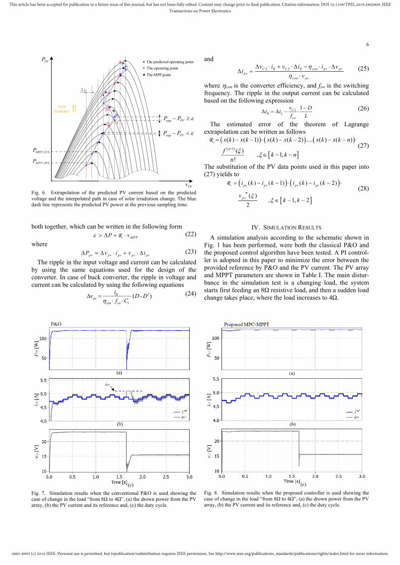
2) Dynamic weather conditions As it can be seen from Fig. 6, during fast solar irradiance

change, each update instant could be from a different PV curve. In this case, the interpolation does not emulate the model of a part of the PV curve. In fact, the interpolation reflects the path of the operating point movement from one PV curve to another. The resulted extrapolated line is shown in blue dashed line, the solid blue line represents the path of the operating point (the blue dashed line may not be seen in some areas where it coincides with the solid one).

If it is assumed that, the voltage reference is increasing and the operating point is on the right side of the MPP point (point A in Fig. 6), the predicted operating point would be B. However, since the prediction on the new PV curve is out of the arced area, the measured power during the next sampling time would be much less than what was expected (point C).

Hence, the predicted power is stored in the controller and labeled as the expected power (Pexp). During the next sampling time, the expected power Pexp is compared to the measured one PPV. If the difference between the measured and expected power exceeds a define threshold (ε), it implies that the operating point has just left the arced area of the PV curve, as shown in Fig. 6. In this case, an opposite action to the one applied during the previous sampling time should applied i.e. if in the last sampling time a voltage/current increment has been added, then, in the current sampling period it should be subtracted, and vice-versa “iPV(k+1)*= iPV(k)*+iPV(k-1)*- iPV(k-2)*”, as illustrated in Fig. 5. By adding this loop to the algorithm, a tracking in the right direction is always fulfilled whether under increasing or decreasing irradiance.

The threshold ε must be greater than the oscillation of the input power of the converter under the same duty ratio and the estimated error of Lagrange polynomial extrapolation added

(18)

(19)

(20)

(21)

1

1( ) ( ) ( ) ( ) ( ) ( ) ( ) ( ) ( )2 2 2 2 2 2

pv pv pv pv pv pv pv pv pva v k - 2 i k i k - 1 v k -1 i k - 2 i k v k i k - 1 i k - 2

( ) ( ) ( ) ( ) ( ) ( ) ( ) ( ) ( ) ( )2 2 2 2 2pv pv pv pv pv pv pv pv pv pvi k - 2 i k - 1 - i k i k - 2 i k - i k - 1 i k - 1 i k i k - 1 i k

2

1( ) ( ) ( ) ( ) ( ) ( ) ( ) ( ) ( )pv pv pv pv pv pv pv pv pva v k - 2 i k - 1 i k v k - 1 i k i k - 2 v k i k - 2 i k - 1

0

1( ) ( ) ( ) ( ) ( ) ( ) ( ) ( ) ( ) ( )

( ) ( ) ( ) ( ) ( )

2 2 2 2pv pv pv pv pv pv pv pv pv pv

2 2pv pv pv pv pv

a v k - 2 i k - 1 i k i k i k - 1 v k - 1 i k - 2 i k i k - 2 i k

v k i k - 2 i k - 1 - i k - 2 i k - 1



6

Fig. 6. Extrapolation of the predicted PV current based on the predicted voltage and the interpolated path in case of solar irradiation change. The blue dash line represents the predicted PV power at the previous sampling time.

both together, which can be written in the following form

MPPP v R (22)

where

pv pv pv pv pvP v i v i (23)

The ripple in the input voltage and current can be calculated by using the same equations used for the design of the converter. In case of buck converter, the ripple in voltage and current can be calculated by using the following equations

1

( )2Rpv

con sw

iv D- D

f C

(24)

Fig. 7. Simulation results when the conventional P&O is used showing the case of change in the load “from 8Ω to 4Ω”, (a) the drown power from the PV array, (b) the PV current and its reference and, (c) the duty cycle.

and 2 2C R C R con pv pv

pvcon pv

v i v i i vi

v

(25)

where conis the converter efficiency, and fsw is the switching frequency. The ripple in the output current can be calculated based on the following expression

2 1CR L

sw

v Di i

f L

(26)

The estimated error of the theorem of Lagrange extrapolation can be written as follows

( 1)

( ) ( 1) ( ) ( 2) .... ( ) ( )

( ), 1,

!

n

x k x k x k x k x k x k n

fk k n

n

R(27)

The substitution of the PV data points used in this paper into (27) yields to

( ) ( 1) ( ) ( 2)

( ), 1, 2

2

pv pv pv pv

pv

i k i k i k i k

vk k

R (28)

IV. SIMULATION RESULTS

A simulation analysis according to the schematic shown in Fig. 1 has been performed, were both the classical P&O and the proposed control algorithm have been tested. A PI control-ler is adopted in this paper to minimize the error between the provided reference by P&O and the PV current. The PV array and MPPT parameters are shown in Table I. The main distur-bance in the simulation test is a changing load, the system starts first feeding an 8Ω resistive load, and then a sudden load change takes place, where the load increases to 4Ω.

Fig. 8. Simulation results when the proposed controller is used showing the case of change in the load “from 8Ω to 4Ω”, (a) the drown power from the PV array, (b) the PV current and its reference and, (c) the duty cycle.

,20MPPP %

,21MPPP %

exp PVP P

exp PVP P

v

PVv

PVP

Solar Irradiance

The operating point

The MPP point

The predicted operating point

A

B

C

D



7

Fig. 9. The irradiance profiles used to assess the dynamic efficiency of the MPPT, according to the standard EN50530. The blue and red colors indicate to the insolation ranges and slopes of low to high solar irradiation test and very low to medium irradiation test, respectively.

The results shown in Fig. 7 and Fig. 8 correspond to P&O

and the proposed MPC-MPPT controller, respectively. As it can be seen from Fig. 7, at the instant 1.75s of the test, where the load suddenly changes, the PI controller takes relatively a long time to adjust the new duty cycle. In this case, the PV array was drifted to operate near the short circuit current (iSC) point, which corresponds to approximately 24W. Moreover, the long response time caused by the PI controller, has led the P&O to make a wrong tracking direction, on account of the operating point is not in the neighborhood of the provided reference. In contrast, since the proposed controller is faster in adjusting the duty cycle, the operating point barely moved from the MPP point during the step load change. One should note, that the oscillation around the provided reference in the classical P&O has been significantly reduced in the proposed MPC-MPPT controller.

V. EXPERIMENTAL RESULTS

A. Test conditions

Different test types have been suggested in the literature for the evaluation of MPPT performances. The well-known test composed of step irradiance changes. But this test does not reflect all the possible weather conditions. Another test consists of a random ramp profile, which emulates a moving clouds also has been suggested. In 2006 a German international working group suggested a standardized MPPT performance test. This test has been approved as a standard in the European Union and published as the Standard EN50530 MPPT performance characterization by the end of 2009 [41].

According to EN50530 standard, the performance of the MPPT is assessed under both static and dynamic conditions. The static test can be performed by running the system under seven defined solar irradiance levels, for a duration of 10 min in each level. The static efficiency can be calculated as function of the European weighting factors by using the following formula

05 10 20

30 50 100....

0.03 0.06 0.13

0.10 0.48 0.2... 0..EU

% % %

% % %

(29)

As well as by using California Energy Commission’s (CEC) weighting factors

10 20 30

50 75 100.....

0.04 0.05 0.12

0...... 21 0.53 0.. 05CEC

% % %

% % %

(30)

where 05% refers to the efficiency of MPPT for a PV array working under 5% of the solar irradiation in standard test conditions. At each irradiance level, the efficiency is calculated based on the following expression

1

1 n

pviav M

P TP T

(31)

where Ppv is the power drawn from the PV string, Pav is the available power in the PV array, TM is the total measurement time, n is the number of periods, and ΔT is the sampling rate. The dynamic efficiency is calculated based on two successive series of a trapezoidal solar irradiance profiles. In the first series, the minimum and maximum of the trapezoidal profiles are 100W/m2 and 500W/m2, respectively. And the ramps are varying from 0.5 W/m2/s in the first sequence (slopeL1) up to 50 W/m2/s in the last sequence (slopeLm) as shown in Fig. 9. Whereas in the second series, the minimum and maximum of the trapezoidal profiles are 300W/m2 and 1000W/m2, respectively. And the ramps are varying from 10 W/m2/s in the first sequence (slopeH1) up to 100 W/m2/s in the last sequence (slopeHm). In each repetition, the efficiency is calculated based on the following product

,1

1

1. .

n

Dyn i pvnj

avj

P TP T

(32)

The dynamic efficiency corresponding to EN50530 standards is the average efficiency of all these repetitions

,1

1 m

Dyn i

n

Dynimn

(33)

where nm is the total number of repetitions.

B. Experimental test bench

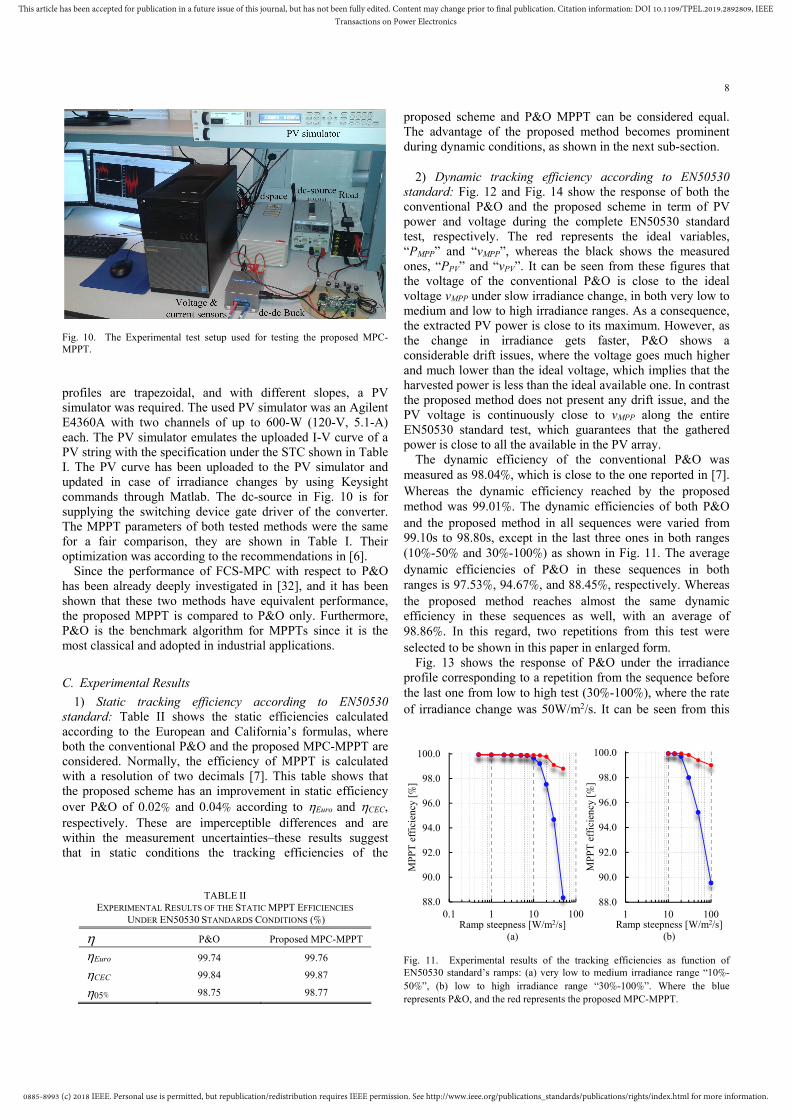
In order to verify the theoretical analysis, experimental tests have been carried out. Fig. 10 shows the experimental test bench used for testing the proposed MPC-MPPT. The control programs have been implemented in Matlab/Simulink, and by using dSPACE real-time interface, they have been compiled and uploaded to dSpace1103 controller board. The converter used here is a 250-W, 35-V prototype buck converter, which has been designed to be installed on the back of a real PV panel for withdrawing the local maximum power. The load was a resistive one (Rload), Rload has been computed in such a way to guarantee a total dissipation greater than the largest PMPP to be evaluated. In this case, Rload has been selected to be 8Ω. Notice that, any converter topology that FCS has been applied to in the literature, can be used here. Furthermore, this system can be connected directly to a dc micro-grid, or to an ac system through an inverter. Since the solar irradiance

TABLE I SIMULATION AND EXPERIMENTAL IMPLEMENTATION PARAMETERS

PV parameters Value Other Parameters Value

Maximum power, PMPP 122W MPPT Frequency, fMPPT 10Hz

Voltage at MPP, vMPP 24.8V Current increment, Δi 0.08A

Open circuit voltage, vOC 31V Switching Frequency, fsw 30kHz

Short circuit current, iSC 5.1A Sampling time, Ts 30µs

Settling

TOP

Down

Sequence 1 (n1 repetition)

Sequence 2 (n2 repetition)

Sequence m (nm repetition)

2/m

st

50%

21

10..

..H

slop

em

21

0..5...

.L

slop

em

2L

slo

pe

2H

slop

e

250

.... .

Lm

s lop

em

210

..0...

.H

msl

ope

m

G. W

100%

10%30%

t

t time



8

88.0

90.0

92.0

94.0

96.0

98.0

100.0

0.1 1 10 100

MP

PT e

ffic

ienc

y [%

]

Ramp steepness [W/m2/s](a)

88.0

90.0

92.0

94.0

96.0

98.0

100.0

1 10 100

MP

PT

eff

icie

ncy

[%]

Ramp steepness [W/m2/s](b)

Fig. 10. The Experimental test setup used for testing the proposed MPC-MPPT.

profiles are trapezoidal, and with different slopes, a PV simulator was required. The used PV simulator was an Agilent E4360A with two channels of up to 600-W (120-V, 5.1-A) each. The PV simulator emulates the uploaded I-V curve of a PV string with the specification under the STC shown in Table I. The PV curve has been uploaded to the PV simulator and updated in case of irradiance changes by using Keysight commands through Matlab. The dc-source in Fig. 10 is for supplying the switching device gate driver of the converter. The MPPT parameters of both tested methods were the same for a fair comparison, they are shown in Table I. Their optimization was according to the recommendations in [6].

Since the performance of FCS-MPC with respect to P&O has been already deeply investigated in [32], and it has been shown that these two methods have equivalent performance, the proposed MPPT is compared to P&O only. Furthermore, P&O is the benchmark algorithm for MPPTs since it is the most classical and adopted in industrial applications.

C. Experimental Results

1) Static tracking efficiency according to EN50530 standard: Table II shows the static efficiencies calculated according to the European and California’s formulas, where both the conventional P&O and the proposed MPC-MPPT are considered. Normally, the efficiency of MPPT is calculated with a resolution of two decimals [7]. This table shows that the proposed scheme has an improvement in static efficiency over P&O of 0.02% and 0.04% according to Euro and CEC, respectively. These are imperceptible differences and are within the measurement uncertainties–these results suggest that in static conditions the tracking efficiencies of the

TABLE II

EXPERIMENTAL RESULTS OF THE STATIC MPPT EFFICIENCIES UNDER EN50530 STANDARDS CONDITIONS (%)

P&O

Proposed MPC-MPPT

Euro

99.74

99.76

CEC

99.84

99.87

05%

98.75

98.77

proposed scheme and P&O MPPT can be considered equal. The advantage of the proposed method becomes prominent during dynamic conditions, as shown in the next sub-section.

2) Dynamic tracking efficiency according to EN50530 standard: Fig. 12 and Fig. 14 show the response of both the conventional P&O and the proposed scheme in term of PV power and voltage during the complete EN50530 standard test, respectively. The red represents the ideal variables, “PMPP” and “vMPP”, whereas the black shows the measured ones, “PPV” and “vPV”. It can be seen from these figures that the voltage of the conventional P&O is close to the ideal voltage vMPP under slow irradiance change, in both very low to medium and low to high irradiance ranges. As a consequence, the extracted PV power is close to its maximum. However, as the change in irradiance gets faster, P&O shows a considerable drift issues, where the voltage goes much higher and much lower than the ideal voltage, which implies that the harvested power is less than the ideal available one. In contrast the proposed method does not present any drift issue, and the PV voltage is continuously close to vMPP along the entire EN50530 standard test, which guarantees that the gathered power is close to all the available in the PV array.

The dynamic efficiency of the conventional P&O was measured as 98.04%, which is close to the one reported in [7]. Whereas the dynamic efficiency reached by the proposed method was 99.01%. The dynamic efficiencies of both P&O and the proposed method in all sequences were varied from 99.10s to 98.80s, except in the last three ones in both ranges (10%-50% and 30%-100%) as shown in Fig. 11. The average dynamic efficiencies of P&O in these sequences in both ranges is 97.53%, 94.67%, and 88.45%, respectively. Whereas the proposed method reaches almost the same dynamic efficiency in these sequences as well, with an average of 98.86%. In this regard, two repetitions from this test were selected to be shown in this paper in enlarged form.

Fig. 13 shows the response of P&O under the irradiance profile corresponding to a repetition from the sequence before the last one from low to high test (30%-100%), where the rate of irradiance change was 50W/m2/s. It can be seen from this Fig. 11. Experimental results of the tracking efficiencies as function of EN50530 standard’s ramps: (a) very low to medium irradiance range “10%-50%”, (b) low to high irradiance range “30%-100%”. Where the blue represents P&O, and the red represents the proposed MPC-MPPT.



9

(b)Time [s]

Pow

er [

W]

Vol

tage

[V

]

P&O

(a)

Fig. 12. (a) The harvested PV power of the conventional P&O during the complete EN50530 standard test, (b) the PV voltage variation of P&O MPPT during the complete EN 50530 standard test.

figure that P&O diverged from the MPP several times. In this situation, P&O diverges until the operating point gets out of the curved area of the P(v) characteristic, where the change in power induced by the perturbation gets larger. The recorded efficiency of P&O in this test was 95.21%. Fig. 15 shows the tracking performance when the proposed MPC-MPPT is applied. As expected, this method has the ability to provide a current reference which continuously matches the operating voltage with vMPP. The proposed scheme shows an efficiency Fig. 13. A repetition from the sequence before the last one from low to high (30%-100%) EN50530 standard test (50W/m2/s), with 5 seconds on top, when P&O is applied. (a) The current used as a reference, (b) the extracted PV power, (c) the PV voltage.

Fig. 14. (a) The harvested PV power of the proposed method during the complete EN50530 standard test, (b) the PV voltage variation of the proposed method during the complete EN 50530 standard test.

of 98.88%, which is improved compared to the conventional P&O by 3.67% in this test.

The second chosen repetition is corresponding to the last sequence from very low to medium test (10%-50%). The speed of the irradiance change in this sequence is 100W/m2/s (Fig. 16 and Fig. 18). It can be observed from Fig. 16 (a), that the conventional P&O is confused due to the fast increase in irradiance. The ideal current iMPP has increased at the fourth second of this test, as a result P&O provided a decreasing

Fig. 15. A repetition from the sequence before the last one from low to high (30%-100%) EN50530 standard test (50W/m2/s), with 5 seconds on top, when the proposed control strategy is applied. (a) The current used as a reference, (b) the extracted PV power, (c) the PV voltage.

(a)Time [s]

Iref

[A

]P

ower

[W

]

Vol

tage

[V

]

Time [s] Time [s](b) (c)

P&O

Proposed MPC-MPPT

(a)

(b)Time [s]

Pow

er [

W]

Vol

tage

[V

]P

ower

[W

]

Vol

tage

[V

]


Proposed MPC-MPPT

(a)Time [s]

Iref

[A

]



10

97.6

98.0

98.4

98.8

99.2

99.6

100.0

-30 -20 -10 0 10 20 30

MP

PT

eff

icie

ncy

[%]

Parameter mismatch [%]

Rload L Rload & L

Fig. 16. A repetition from the last sequence from very low to medium (10%-50%) EN50530 standard test (100W/m2/s), with 5 seconds on top, when P&O is applied. (a) the current used as a reference, (b) the extracted PV power, (c) the PV voltage.

reference, which caused to a much higher PV voltage than vMPP. Also, during the decrease of the irradiance, the P&O reference has been confused, and stayed on the top of the ramp, while the ideal iMPP has started to decrease. Due to the voltage drift during both the fast increase and fast decrease of the irradiance in this sequence, the efficiency of P&O barely reaches 88.33%. From Fig. 18, it can be seen that the proposed approach is still robust even under such a fast irradiance increase, in fact, it provides a non-confused reference, conforming with the ideal one, and the harvested PV power was at its maximum during the whole profile. The efficiency of the proposed MPC-MPPT in this test is 98.85%, which is improved over P&O by 10.52%.

3) Model parameter mismatch: One of the drawbacks of MPC schemes is the effect of model parameters misestimation on the controller performance.

Fig. 17. Experimental results of the proposed approach under the STC in case of model parameter mismatch, “Rload, and L”.

Fig. 18. A repetition from the last sequence from very low to medium (10%-50%) EN50530 standard test (100W/m2/s), with 5 seconds on top, when the proposed MPC-MPPT is applied. (a) the current used as a reference, (b) the extracted PV power, (c) the PV voltage.

Hence, the proposed MPC-MPPT has been also tested with mismatched model parameters, where the range of modeling errors was ±30%. Note that the system was operating under the STC in this test. It can be seen from the results displayed in Fig. 17, that the effect of the underestimation of the load resistor by 30% drops the efficiency to 99.01%, while the same mismatch of the inductor value worsens the efficiency to 98.40%. One should note that, the effect of mismatched load resistor is less than the effect of mismatched inductor.

From Fig. 17, it can be observed that the effect of -30%

mismatched inductor leads to a drop of the efficiency to 97.89%, whereas +30% mismatch exhibits a drop to 98.45%. It can be noted that, the mismatch of the inductor value, is asymmetrical, i.e., the underestimation of this parameter has more influence than its overestimation on the MPPT efficiency. And it is the case with the resistor as well.

VI. CONCLUSION

An MPC-based MPPT for rapidly changing meteorological conditions has been presented in this paper. The method estimates the PV current/voltage that should be applied in order to make the operating point converge to the MPP. Moreover, it has the ability to detect whether the operating point is still at PMPP, or it has been deviated e.g. due to a fast change in the environmental conditions. The estimated PV current/voltage serves as a reference to finite control set MPC, and the switching state that minimizes the difference between this reference and the predicted variable is applied directly to the converter. The proposed method has been implemented and compared to the conventional P&O according to EN50530

(a)Time [s]

Vol

tage

[V

]


Iref

[A

]P

ower

[W

]

P&O

(a)Time [s]

Vol

tage

[V

]


Iref

[A

]P

ower

[W

]

Proposed MPC-MPPT



11

in both static and dynamic conditions. The experimental results show that the proposed scheme offers an excellent dynamic performance with respect to P&O algorithm, providing a reference that matches the MPP locus even under very fast environmental condition changes.

VII. REFERENCES [1] Fernandes D, Almeida R, Guedes T, Sguarezi Filho AJ, Costa FF. "State

feedback control for DC-photovoltaic systems," Electric Power Systems Research. vol. 143, pp. 794-801. Feb. 2017.

[2] T. Esram and P. L. Chapman, "Comparison of photovoltaic array maximum power point tracking techniques," IEEE Trans. Energy Convers., vol. 22, pp. 439-449, June 2007.

[3] A. Lashab, A. Bouzid and H. Snani, "Comparative study of three MPPT algorithms for a photovoltaic system control," 2015 World Congr. Info. Technol. Comput. Appl. WCITCA 2015, no. 3, 2015.

[4] J. Kivimäki, S. Kolesnik, M. Sitbon, T. Suntio and A. Kuperman, "Revisited Perturbation Frequency Design Guideline for Direct Fixed-Step Maximum Power Point Tracking Algorithms," IEEE Trans. Ind. Electron, vol. 64, no. 6, pp. 4601-4609, June 2017.

[5] F. Paz and M. Ordonez, "High-Performance Solar MPPT Using Switching Ripple Identification Based on a Lock-In Amplifier," IEEE Trans. Ind. Electron., vol. 63, no. 6, pp. 3595-3604, June 2016.

[6] N. Femia, G. Petrone, G. Spagnuolo, M. Vitelli, "Optimization of perturb and observe maximum power point tracking method," IEEE Trans. Power Electron. vol. 20, no. 4, pp. 963-973, July 2005.

[7] D. Sera, L. Mathe, T. Kerekes, S. V. Spataru, and R. Teodorescu, " On the Perturb-and-Observe and Incremental Conductance MPPT Methods for PV Systems," IEEE J. Photovolt., vol. 3, no. 3, pp. 1070–1078, 2013.

[8] J. Ahmad, "A fractional open circuit voltage based maximum power point tracker for photovoltaic arrays," 2nd Int.l Conf. Software Technol. Engineering, San Juan, PR, 2010, pp. V1-247-V1-250.

[9] M. Killi and S. Samanta, "Modified Perturb and Observe MPPT Algorithm for Drift Avoidance in Photovoltaic Systems," IEEE Trans. Ind. Electron., vol. 62, no. 9, pp. 5549-5559, Sept. 2015.

[10] D. Sera, R. Teodorescu, J. Hantschel and M. Knoll, "Optimized Maximum Power Point Tracker for Fast-Changing Environmental Conditions," IEEE Trans. Ind. Electron., vol. 55, no. 7, pp. 2629-2637, July 2008.

[11] J. Ahmed and Z. Salam, "A Modified P&O Maximum Power Point Tracking Method With Reduced Steady-State Oscillation and Improved Tracking Efficiency," IEEE Trans. Sust. Energy, vol. 7, no. 4, pp. 1506-1515, 2016.

[12] G. Escobar, S. Pettersson, C. N. M. Ho and R. Rico-Camacho, "Multisampling Maximum Power Point Tracker (MS-MPPT) to Compensate Irradiance and Temperature Changes," IEEE Trans. Sust. Energy, vol. 8, no. 3, pp. 1096-1105, July 2017.

[13] S. K. Kollimalla and M. K. Mishra, “Variable perturbation size adaptive P&O MPPT algorithm for sudden changes in irradiance,” IEEE Trans. Sust. Energy, vol. 5, no. 3, pp. 718–728, Jul. 2014.

[14] H. A. Sher, A. F. Murtaza, A. Noman, K. E. Addoweesh, K. Al-Haddad and M. Chiaberge, “A New Sensorless Hybrid MPPT Algorithm Based on Fractional Short-Circuit Current Measurement and P&O MPPT,” IEEE Trans. Sust. Energy, vol. 6(4), pp. 1426-1434, October 2015.

[15] B. N. Alajmi, K. H. Ahmed, S. J. Finney and B. W. Williams, "A Maximum Power Point Tracking Technique for Partially Shaded Photovoltaic Systems in Microgrids," IEEE Trans. Ind. Electron., vol. 60, no. 4, pp. 1596-1606, April 2013.

[16] S. Messalti, A. G. Harrag and A. E. Loukriz, "A new neural networks MPPT controller for PV systems," The Sixth Int. Renewable Energy Congrs (IREC), Sousse, 2015, pp. 1-6.

[17] E. Bianconi, J. Calvente, R. Giral, E. Mamarelis, G. Petrone, C. A. Ramos-Paja, Giovanni Spagnuolo, Senior Member, IEEE, and Massimo Vitelli "A Fast Current-Based MPPT Technique Employing Sliding Mode Control," IEEE Trans. Ind. Electron., vol. 60, no. 3, pp. 1168-1178, March 2013.

[18] S. Vazquez, J. I. Leon, L. G. Franquelo, J. Rodriguez, H. A. Young, A. Marquez, and P. Zanchetta, “Model predictive control. A review of its applications in power electronics,” IEEE Ind. Electron. Mag., vol. 8, no. 1, pp. 16–31, Mar. 2014.

[19] A. Linder, R. Kanchan, R. Kennel, and P. Stolze, "Model Based Predictive Control of ElectricDrives," Germany: Cuvillier Verlag Göttingen, 2010.

[20] W. Song, Y. Zhang, X. Sun, Q. Zhang, and W. Wang, “A study of Zsource dual-bridge matrix converter immune to abnormal input voltage disturbance and with high voltage transfer ratio,” IEEE Trans. Ind. Info., vol. 9, no. 2, pp. 828–838, May 2013.

[21] P. Cortes, M. P. Kazmierkowski, R. M. Kennel, D. E. Quevedo, and J. Rodriguez, “Predictive control in power electronics and drives,” IEEE Trans. Ind. Electron., vol. 55, no. 12, pp. 4312–4324, Dec. 2008.

[22] J. Rodriguez, M. P. Kazmierkowski, J. R. Espinoza, P. Zanchetta, H. Abu-Rub, H. A. Young, et al., "State of the Art of Finite Control Set Model Predictive Control in Power Electronics," IEEE Trans. Ind. Info, vol. 9, pp. 1003-1016, 2013.

[23] R. Errouissi, S. M. Muyeen, A. Al-Durra, and Siyu Leng. "Experimental Validation of a Robust Continuous Nonlinear Model Predictive Control Based Grid-Interlinked Photovoltaic Inverter." IEEE Trans. Ind. Electron., vol, 63.no 7: pp. 4495-4505. July 2016.

[24] R. Erase, S. M. Muyeen, A. Al-Durra, and S. Leng. "A Robust Continuous-Time MPC of a DC–DC Boost Converter Interfaced With a Grid-Connected Photovoltaic System." IEEE J. Photovolt., vol. 6, no. 6: pp. 1619-1629, 2016.

[25] M. B. Shadmand, X. Li, R. S. Balog and H. A. Rub, "Model predictive control of grid-tied photovoltaic systems: Maximum power point tracking and decoupled power control," First Workshop on Smart Grid and Renewable Energy (SGRE), Doha, 2015, pp. 1-6.

[26] M. Metry; M. B. Shadmand; R. S. Balog; H. A. Rub, "MPPT of Photovoltaic Systems Using Sensorless Current-Based Model Predictive Control,"IEEE Trans. Ind. App., vol. 53, no. 2, pp. 1157-1167, Ap 2017.

[27] O. Abdel-Rahim and H. Funato, "Model Predictive Control based Maximum Power Point Tracking technique applied to Ultra Step-Up Boost Converter for PV applications," IEEE Innovative Smart Grid Technol., Asia (ISGT ASIA), Kuala Lumpur, 2014, pp. 138-142.

[28] M. B. Shadmand, M. Mosa, R. S. Balog and H. A. Rub, "An improved MPPT technique for high gain DC-DC converter using model predictive control for photovoltaic applications," IEEE Applied Power Electro. Conf. and Expo., APEC 2014, Fort Worth, pp. 2993-2999.

[29] M. Mosa, M. B. Shadmand, R. S. Balog and H. Abu Rub, "Efficient maximum power point tracking using model predictive control for photovoltaic systems under dynamic weather condition," IET Renewable Power Generation, vol. 11, no. 11, pp. 1401-1409, 9 13 2017.

[30] S. Sajadian, R. Ahmadi, "Model Predictive-Based Maximum Power Point Tracking for Grid-Tied Photovoltaic Applications Using a Z-Source Inverter," IEEE Trans. Power Electron., vol. 31, no. 11, pp. 7611–7619, Nov. 2016.

[31] A. A. Abushaiba, S. M. M. Eshtaiwi and R. Ahmadi, "A new model predictive based Maximum Power Point Tracking method for photovoltaic applications," 2016 IEEE Int. Conf. Electro Info. Technol. (EIT), Grand Forks, ND, pp. 0571-0575.

[32] A. Lashab, D. Sera, J. M. Guerrero, L. Mathe and A. Bouzid, "Discrete Model-Predictive-Control-Based Maximum Power Point Tracking for PV Systems: Overview and Evaluation," IEEE Trans. Power Electron., vol. 33, no. 8, pp. 7273-7287, Aug. 2018.

[33] P. S. Shenoy, M. Amaro, J. Morroni and D. Freeman, "Comparison of a Buck Converter and a Series Capacitor Buck Converter for High-Frequency, High-Conversion-Ratio Voltage Regulators," IEEE Trans. Power Electron., vol. 31, no. 10, pp. 7006-7015, Oct. 2016.

[34] P. Karamanakos, T. Geyer and S. Manias, "Direct Voltage Control of DC–DC Boost Converters Using Enumeration-Based Model Predictive Control," IEEE Trans. Power Electron., vol. 29, no. 2, pp. 968-978, Feb. 2014.

[35] P. Cortes et al., “Guidelines for weighting factors design in model predictive control of power converters and drives,” in Proc. IEEE Int. Conf. Ind. Technol., Feb. 2009, pp. 1–7.

[36] T. Dragicevic and M. Novak, "Weighting Factor Design in Model Predictive Control of Power Electronic Converters: An Artificial Neural Network Approach," IEEE Trans. Ind. Electron.. Accepted, doi: 10.1109/TIE.2018.2875660

[37] Z. Zhang, W. Tian, W. Xiong, and R. Kennel, “Predictive torque control of induction machines fed by 3L-NPC converters with online weighting factor adjustment using Fuzzy Logic,” in Proc. IEEE Transport. Electrification Conf. Expo, Jun. 2017, pp. 84–89.

[38] Higham, N. J. (1988). "Fast Solution of Vandermonde-Like Systems Involving Orthogonal Polynomials". IMA Journal of Numerical Analysis. 8 (4): 473–486.



12

[39] Calvetti, D & Reichel, L (1993). "Fast Inversion of Vanderomnde-Like Matrices Involving Orthogonal Polynomials". BIT. 33 (33): 473–484. doi:10.1007/BF01990529.

[40] M. E. Ropp, S Gonzalez. “Development of a MATLAB/Simulink modelof a single phase grid-connected photovoltaic system.” IEEE Trans. Energy Convers., vol. 24, no. 1: pp. 195-202, 2009.

[41] H. Häberlin, P. Schärf, “New test procedure for Measuring Dynamic MPP Tracking Efficiency at Grid connected PV inverters”, 24th European Photovoltaic Solar Energy Conf., Germany, Sep 2009, pp. 3631-3637.

[42] H. Schmidt, B. Burger, U. Bussemas, & S. Elies, “How fast does an MPP tracker really need to be?” 24th European Photovoltaic Solar Energy Conference, Hamburg, Germany, Jan 2009, pp. 3273-3276.

Abderezak Lashab (S’13) received the bachelor’s and master’s degrees in electrical engineering in 2010 and 2012, respectively, from Universié des Frères Mentouri Constantine, Constantine, Algeria. During the year 2013, he served as an engineer in High Tech Systems (HTS).

He is currently working toward the Ph.D. degree with the Department of Energy technology, Aalborg University, Denmark. His current research interests include control, modeling, and diagnostics of

photovoltaic power systems, and power electronics.

Dezso Sera (S’05–M’08–SM’15) received the B.Sc. and M.Sc. degrees in electrical engineering from the Technical University of Cluj, Cluj-Napoca, Romania, in 2001 and 2002, respectively, the M.Sc. degree in power electronics and the Ph.D. degree in PV systems from the Department of Energy Technology, Aalborg University, Aalborg, Denmark, where he is currently an Associate Professor. Since 2009, he has been Programme

Leader of the Photovoltaic Systems Research Programme (www.pv-systems.et.aau.dk) at the same department.

His research interests include modeling, characterization, diagnostics and maximum power point tracking (MPPT) of PV arrays, as well as power electronics, and grid integration for PV systems.

Josep M. Guerrero (S’01–M’04–SM’08–F’15) received the B.S. degree in telecommunications engineering, the M.S. degree in electronics engineering, and the Ph.D. degree in power electronics from the Technical University of Catalonia, Barcelona, Spain, in 1997, 2000, and 2003, respectively. Since 2011, he has been a Full Professor with the Department of Energy Technology, Aalborg University, Aalborg,

Denmark, where he is responsible for the Microgrid Research Program. In 2012, he was a Guest Professor with the Chinese Academy of Science and the Nanjing University of Aeronautics and Astronautics; and in 2014, he was the Chair Professor with Shandong University.

His research interests include different microgrid aspects, including power electronics, distributed energy-storage systems, hierarchical and cooperative control, energy management systems, and optimization of microgrids and islanded minigrids.

Dr. Guerrero was awarded by Thomson Reuters as an ISI Highly Cited Researcher

a dual-discrete model predictive control-based mppt for pv

Documents