Model predictive control for vehiclesteering using road information in thelocal frameMaster’s thesis in Systems, Control and Mechatronics

LOVE MOWITZNAM VU

Department of Mechanics and Maritime SciencesCHALMERS UNIVERSITY OF TECHNOLOGYGoteborg, Sweden 2019

MASTER’S THESIS IN SYSTEMS, CONTROL AND MECHATRONICS

Model predictive control for vehicle steering using road information in thelocal frame

LOVE MOWITZNAM VU

Department of Mechanics and Maritime Sciences

Division of Vehicle Engineering and Autonomous Systems

CHALMERS UNIVERSITY OF TECHNOLOGY

Goteborg, Sweden 2019

Model predictive control for vehicle steering using road information in the local frameLOVE MOWITZNAM VU

c© LOVE MOWITZ, NAM VU, 2019

Master’s thesis 2019:81Department of Mechanics and Maritime SciencesDivision of Vehicle Engineering and Autonomous SystemsChalmers University of TechnologySE-412 96 GoteborgSwedenTelephone: +46 (0)31-772 1000

Chalmers ReproserviceGoteborg, Sweden 2019

Model predictive control for vehicle steering using road information in the local frameMaster’s thesis in Systems, Control and MechatronicsLOVE MOWITZNAM VUDepartment of Mechanics and Maritime SciencesDivision of Vehicle Engineering and Autonomous SystemsChalmers University of Technology

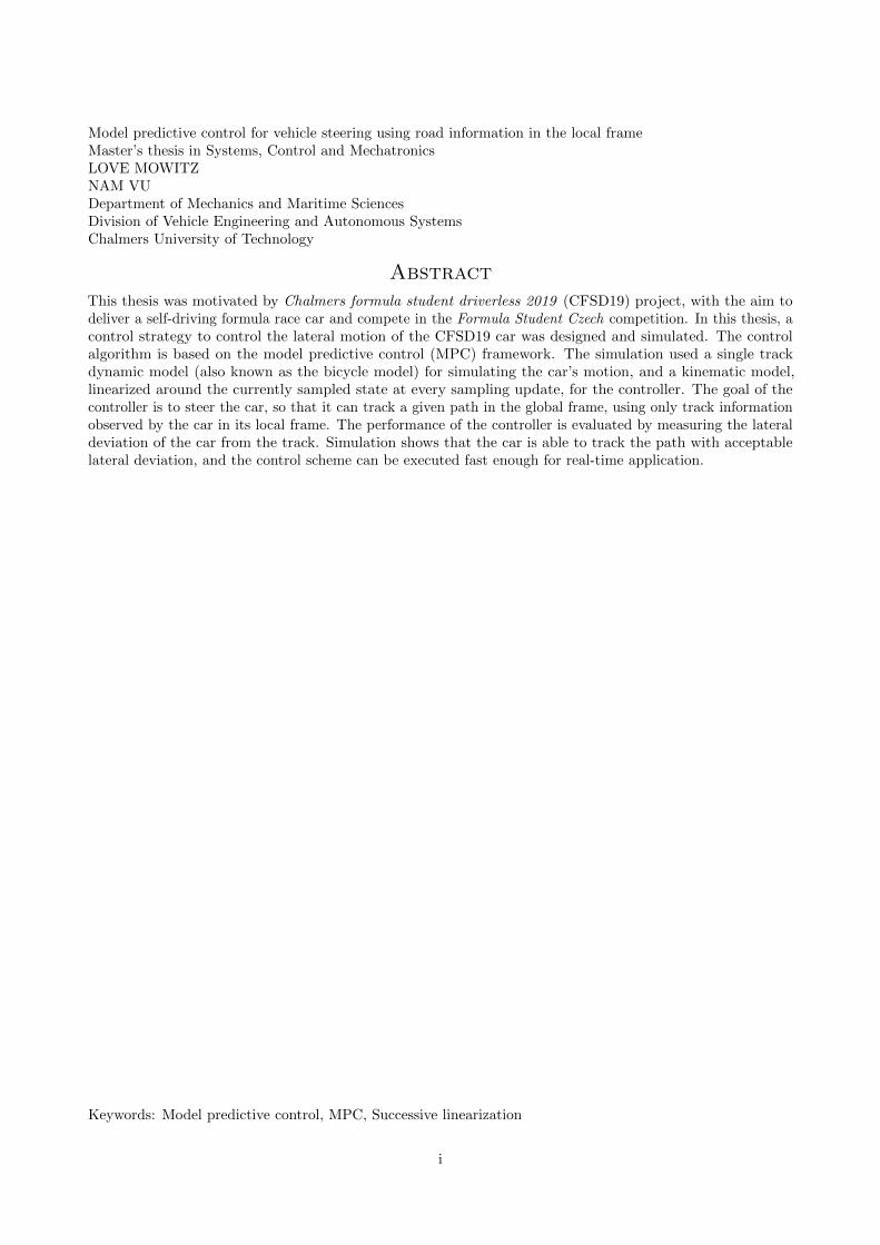
AbstractThis thesis was motivated by Chalmers formula student driverless 2019 (CFSD19) project, with the aim todeliver a self-driving formula race car and compete in the Formula Student Czech competition. In this thesis, acontrol strategy to control the lateral motion of the CFSD19 car was designed and simulated. The controlalgorithm is based on the model predictive control (MPC) framework. The simulation used a single trackdynamic model (also known as the bicycle model) for simulating the car’s motion, and a kinematic model,linearized around the currently sampled state at every sampling update, for the controller. The goal of thecontroller is to steer the car, so that it can track a given path in the global frame, using only track informationobserved by the car in its local frame. The performance of the controller is evaluated by measuring the lateraldeviation of the car from the track. Simulation shows that the car is able to track the path with acceptablelateral deviation, and the control scheme can be executed fast enough for real-time application.

Keywords: Model predictive control, MPC, Successive linearization

i

ii

AcknowledgementsFirst and foremost, we would like to express our sincere gratitude towards our examiner, Ola Benderius, forhis guide and support during both the project and thesis. Our gratitude also extends to all the members ofCFSD19 team who have worked with us in the project. In addition, we would also like to thank the members ofthe CFSD18 and CFS17 team, our predecessors, who built the car and laid the foundation for the current project.

Last but not least, we also want to thank the staff of Revere lab, including Arpit Karsolia, Fredrik vonCorswant, Christian Berger and many others, for sharing their resources and offering valuable help throughoutthe project.

Thesis examiner: Ola Benderius

iii

iv

Contents

Abstract i

Acknowledgements iii

Contents v

1 Introduction 11.1 Aim . . . . . . . . . . . . . . . . . . . . . . . . . . . . . . . . . . . . . . . . . . . . . . . . . . . . . 11.2 Scope . . . . . . . . . . . . . . . . . . . . . . . . . . . . . . . . . . . . . . . . . . . . . . . . . . . . 1

2 Background 3

3 Theory 63.1 Model predictive control . . . . . . . . . . . . . . . . . . . . . . . . . . . . . . . . . . . . . . . . . . 63.2 Successive linearization of controller model . . . . . . . . . . . . . . . . . . . . . . . . . . . . . . . 73.2.1 Discretization . . . . . . . . . . . . . . . . . . . . . . . . . . . . . . . . . . . . . . . . . . . . . . . 83.3 Quadratic programming formulation . . . . . . . . . . . . . . . . . . . . . . . . . . . . . . . . . . . 8

4 Method 134.1 Simulation setup . . . . . . . . . . . . . . . . . . . . . . . . . . . . . . . . . . . . . . . . . . . . . . 134.2 Simulation of vehicle motion . . . . . . . . . . . . . . . . . . . . . . . . . . . . . . . . . . . . . . . 144.2.1 Equations of motion . . . . . . . . . . . . . . . . . . . . . . . . . . . . . . . . . . . . . . . . . . . 144.2.2 Lateral tire forces . . . . . . . . . . . . . . . . . . . . . . . . . . . . . . . . . . . . . . . . . . . . 164.2.3 Longitudinal tire forces . . . . . . . . . . . . . . . . . . . . . . . . . . . . . . . . . . . . . . . . . 164.2.4 Load transfer . . . . . . . . . . . . . . . . . . . . . . . . . . . . . . . . . . . . . . . . . . . . . . . 184.3 Reference path generation . . . . . . . . . . . . . . . . . . . . . . . . . . . . . . . . . . . . . . . . . 194.3.1 Generating reference path from local path . . . . . . . . . . . . . . . . . . . . . . . . . . . . . . . 194.4 Longitudinal control . . . . . . . . . . . . . . . . . . . . . . . . . . . . . . . . . . . . . . . . . . . . 204.5 Lateral control . . . . . . . . . . . . . . . . . . . . . . . . . . . . . . . . . . . . . . . . . . . . . . . 214.5.1 Kinematic model . . . . . . . . . . . . . . . . . . . . . . . . . . . . . . . . . . . . . . . . . . . . . 214.5.2 Dynamic model . . . . . . . . . . . . . . . . . . . . . . . . . . . . . . . . . . . . . . . . . . . . . . 224.5.3 Torque vectoring . . . . . . . . . . . . . . . . . . . . . . . . . . . . . . . . . . . . . . . . . . . . . 24

5 Results 265.1 Controller specifications . . . . . . . . . . . . . . . . . . . . . . . . . . . . . . . . . . . . . . . . . . 265.2 Steady state cornering . . . . . . . . . . . . . . . . . . . . . . . . . . . . . . . . . . . . . . . . . . . 265.3 Double lane change . . . . . . . . . . . . . . . . . . . . . . . . . . . . . . . . . . . . . . . . . . . . . 275.4 Track drive . . . . . . . . . . . . . . . . . . . . . . . . . . . . . . . . . . . . . . . . . . . . . . . . . 30

6 Discussion 33

7 Conclusions 357.1 Future work . . . . . . . . . . . . . . . . . . . . . . . . . . . . . . . . . . . . . . . . . . . . . . . . . 35

References 36

v

vi

1 Introduction

Autonomous driving technology is currently an active field of study, and is expected to change the automotiveindustry in the near future. Sharing the same vision, Formula Student Germany (FSG), an engineering designcompetition where students build their own formula racing cars to compete with others, has also adoptedFormula Student Driverless as a new competition class since 2017, and by 2021, “all vehicles participatingin FSG are supposed to have driverless technology on board” [1]. Given the rising interest in autonomousvehicles in this area, it is of interest to investigate different controller performances on an autonomous race vehicle.

In 2017, the same year as the first FSG competition with a driverless class, Chalmers University of Technologyset up a Formula Student Driverless team. Chalmers Formula Student Driverless (CFSD) thus had it’s firstseason in 2018 where the members converted a manually driven formula race car into a driverless vehicle. Atthe competition the vehicle races in four different dynamic events meant to test the vehicle’s ability to navigatethrough the specified track environment. The event tracks are marked with colored cones and are designed totest the full capabilities of the vehicles.

This thesis investigates the lateral control of a formula car developed for use in the CFSD19 car and as suchtakes into account the dynamic events of driverless competitions when evaluating the controller. The proposedlateral controller utilises decoupled model predictive control (MPC) with two different system controller modelsand its performance is simulated using a two-track vehicle model. The decoupled MPC controllers usingdifferent controller plant models are simulated using test cases to provide insight on the controller performancein conditions comparable to the Formula Student competition dynamic events. To provide a simulation of thelateral controller in the context of the real system, the path planning and longitudinal control planned for thevehicle is additionally part of the simulation environment.

1.1 Aim

The aim of this thesis is to investigate the feasibility of a decoupled MPC for the steering of a Formula Studentcar. Specifically, this thesis aims to answer the following research questions:

• What is the performance of a decoupled MPC for steering in the specified driving environment?

• What is the performance effect of different controller plant models for the decoupled MPC in the specifieddriving environments?

1.2 Scope

This thesis will not investigate the implications coupled lateral and longitudinal control and will instead onlyconsider decoupled lateral control at varying longitudinal speeds using different plant models. The vehiclemodel will also be tailored to the specific Formula Student car developed in 2017 by Chalmers Formula Studentwhich was made autonomous in 2018 by Chalmers Formula Student Driverless. The Formula Student Driverlesscompetition tracks and track setup will also be taken into consideration when testing and evaluating thecontroller.

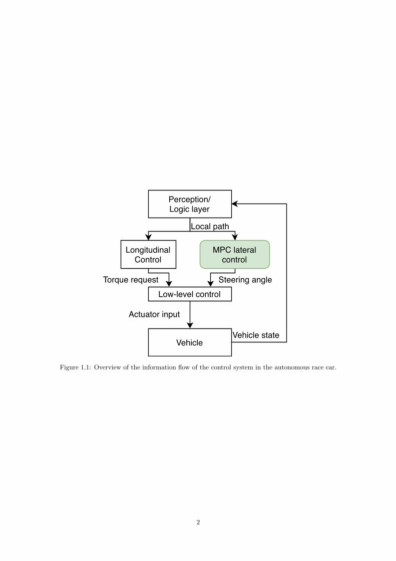
The proposed controller sits between the perception and low-level controllers that interface with the steeringactuation. Figure 1.1 shows an overview of the system architecture and where the focus of this thesis lies.

1

Perception/Logic layer

MPC lateralcontrol

Low-level control

Vehicle

Steering angle

Local path

Vehicle state

Actuator input

LongitudinalControl

Torque request

Figure 1.1: Overview of the information flow of the control system in the autonomous race car.

2

2 Background

Model predictive control is an advanced method for process control able to satisfy given input and outputconstraints and can therefore be useful for safety critical autonomous design [2]. MPC was originally developedin the context of power plants and petroleum refineries but can today be found in a wide variety of areas,including the automotive industry [3][4]. This can be attributed to the growing processing power increasing thepossibility of real time application in some areas. This has also made it possible for non-linear MPC solutionsto be feasible in real time in some cases [5]. Since MPC is model-based control, it is similar to a linear-quadraticregulator (LQR). MPC, however, differs from LQR in that a finite time-horizon is optimized but only thefirst input is used from the optimal control sequence and then the process is optimized again at the next time step.

One specific area of MPC application in automotive control is called Active Front Steering (AFS). In thisapplication, MPC is used to adjust the front steering angle of vehicles, without changing the position of steeringwheel. This is used to assist the driver around difficult cornering in non-autonomous driving. Using MPCallows the controller to account for physical constraints, such as maximum steer angle or maximum steeringrate. This was demonstrated by Yoon et al. [6], or Falcone [7]. The positive results as well as the simple setupfor these controllers gave motivation of the this thesis.

Since MPC is a model-based control scheme, it is therefore important to choose the right model to predict thevehicle motion. There are generally three types of models for vehicle control: kinematic model which describesvehicle motion by only examining its velocities and orientation; single-track (or bicycle) dynamic model whichcollapses a four-wheel vehicle into only two wheels in a single axis, and describes vehicle motions using forcesand inertia (linear or rotational) of vehicle; and two-track model which is similar to single-track model but nowexamine all four wheels and also account for the vehicle’s rolling motion. Each model has its own advantagesand drawbacks, and the right model is the best compromise between its accuracy in describing motion, andits complexity. The first class of model, kinematic model is considered to be simplest and would require lesscomputational power, which is beneficial for real-time application. This model also avoids the singular problemin tire modelling, namely that tire model have a tire slip angle equation which has the longitudinal velocity inthe denominator (thus making tire model unusable at zero or low velocity). However, the biggest drawbackof kinematic model is its inaccuracy particularly under high longitudinal speed or high lateral acceleration.In one report [8], a comparison in the accuracy of predicting a vehicle position between a kinematic and adynamic-based MPC steering was done. The result showed that a kinematic model gives worse predictionover time compared to a dynamic one, particularly in high speed. Thus in high dynamic application such ascontrolling a racing car, it is deemed better to use a dynamic model for controller. In another report [9], anextensive comparison of accuracy between different car dynamic models were done: namely a single track modelwith three different tire models (linear, nonlinear magic formula, and tire force lag), and a two-track model. Theoutputs of these models (front side slip angle, yaw rate) were compared against real measurements in a doublelane change test, where the test car was driven at three different speeds (36, 49, and 59 km/h). It was concludedthat a single track model with tire for lag model would perform equally well as a two-track model, and the single-track, linear-tire model would perform well only up to a lateral acceleration of 0.5G. Thus the conclusion fromthis is that it is good enough to use a single track model, as long as the tire model is good enough for the use case.

In case of dynamics-model-based controller, one usually consider whether to couple or decouple the controlstrategy. A decoupled dynamic controller is a control strategy where the longitudinal and lateral dynamics ofvehicles are separately controlled by two separate controller; whereas in coupled controllers both dynamicsare controlled by a single controller. The industry practice for path tracking MPC is to decouple longitudinaland lateral dynamics, in which a speed profile (that aims at maximize acceleration capability for example)is generated first; and the longitudinal controller (MPC or PID) would make sure the car drives at the setspeed. After that, another separate controller would use the longitudinal set speed as a parameter, and makesure the car follow a desired lateral trajectory (lane keeping or collision avoidance for example). Coupledcontrollers are generally more complex to implement, but they give better performance in theory. Severalattempts have been made to implement and study coupled dynamic controllers. Both coupled and decoupleddynamic model based controllers have been discussed prominently in other reports [10][11]. One proposeddesign was a coupled controller, where longitudinal and lateral dynamics were controlled separately but theyexchange information together while having to satisfy the same constraint on tire slip angle [11]. Extensive work

3

regarding comparing coupled and decoupled controllers in terms of both performance, complexity and executiontime has likewise been done before. In one such report [12], both controllers used a single track dynamic model,with the decoupled controller controlling only the steering angle, while the coupled one controlling both thesteering angle and longitudinal acceleration. The author concluded that the coupled controller only performedslightly better than the decoupled one in terms of lateral tracking (the difference is only 1 cm lateral deviationless for the coupled one). However, the coupled one is more complex and harder to tune, and it also takes quitemore time to execute (the average control loop of the coupled one being 11 ms, 2 ms more than the decoupledone, and this violated a requirement of 10 ms control loop in this work). Figure 2.1 illustrates the comparisonof coupled and decoupled controllers done in the previously mentioned report [12]. Based on these results, thedecoupled control scheme was chosen in this thesis.

Figure 2.1: Comparison between coupled and decoupled controller [12].

In a model predictive control scheme, at each control step an optimization problem is solved based on someperformance index (minimising or maximizing a cost function), and this is repeated for every control step. Theoptimization problem can be based on a linear or non-linear model with respect to the optimizing variables.Even though a non-linear model is usually more accurate than a linear one, it often results in a more complexnonlinear programming problem, and takes more to to solve. This would contradict the real-time requirement ofmost control problems. Therefore, many MPC application in autonomous driving would linearize the non-linearcontrol models at the current operating conditions, to get an approximation of the nonlinear model, anduse that linearized model for the MPC-solver. This is called successive linearization, and the optimizationproblem of this kind is called Linear-Time Varying model MPC, or LTV-MPC. LTV-MPC are commonly usedin autonomous driving application, due to most dynamic models for lateral control being nonlinear with respectto both states and control inputs.

Other authors have previously proposed an LTV-MPC for active front steering, where a discrete-time, linearsystem was obtained by successive online linearization of a nonlinear vehicle mode [7][13]. Also in these works,the stability conditions for LTV-MPC controllers were presented. In a similar report the authors have alsodemonstrated that successive linearizations of a nonlinear model over the prediction horizon would improve theaccuracy of the LTV prediction model and thus the performance of the controller [14]. Outside of applicationsfor automotive autonomous control, successive linearization are also widely applied in other fields, such asrobotics or in marine vessel tracking [15][16]. The results from the aforementioned works showed that LTV-MPCare robust for active front steering control, and thus an LTV-MPC obtained from successful linearization waschosen in this thesis.

4

After the controller is designed, it is also important to decide how it would be tested. Controller validationdepends greatly on the selected test scenarios. For a racing car, it is desirable to examine the controllerbehaviour at its limiting conditions. One report investigates different test scenarios and their benefits [17].Based on this work, the following tests were chosen in this thesis:

• Steady state cornering: The vehicle drives in a constant radius turn. The radius is the same as theturning radius in the skidpad dynamic event. The vehicle would drive at different constant longitudinalvelocities. Lateral deviation from middle line of the test track would be recorded. This test would revealinformation about the vehicle’s under or over-steering properties.

• Double lane change: The vehicle drives in a first straight lane for 50 m, then steer sideways and changeto a second lane. It continues on that lane for 12 m, then steer back to the first lane and continue drivingon the first lane until the end. The lanes are three meters apart. This test is commonly used for testingelectronic control systems (ECS).

• Track drive: The vehicle drives in a track following the Formula Student Driverless track drive ruleswhich includes straights, constant turns and hairpin turns. The lanes are three meters apart. The test isused to provide insight to the controller performance in the intended application environment.

Last but not least, time complexity is a major consideration when implementing MPC. Due to the fast dynamicnature of vehicle dynamics, any controller must be able to execute control loops fast enough. In most of theworks mentioned above, MPC controllers were able to run at a relatively high frequency, from 50 hz and above.Thus, in this thesis, it is of importance that the controller design enables a high control frequency in terms ofcomplexity. It is however important to keep in mind that the intended execution environment on the formulacar will have limited resources that have to be shared among multiple programs and that the controller shouldalso be evaluated at lower control loop frequencies.

5

3 Theory

This chapter provides the necessary background for understanding the controller formulation and design. Theoryabout LTV MPC is presented through a general MPC formulation with the linearization and discretization ofnon-linear system dynamics.

3.1 Model predictive control

Model predictive control is well suited for system where safety requirements have to be considered, such as lanekeeping for vehicle control. Some of the advantages of MPC is constraint handling, explicit use of a model andwell defined tuning parameters together with its ability to take future system behaviour into consideration. Bythis it is possible to, for example, take wheel angle and road lane limits into consideration when formulatingthe problem, which is also taken into consideration when evaluating future system behavior.

MPC is based on a finite-horizon optimization of a dynamic system by utilizing a mathematical model of theplant. The current state of the system is sampled at time t and minimizes a cost function based on the systemstates and inputs between the current sampled time until some point in the future t+ T divided into N steps.A basic MPC formulation can be expressed as

minuJ(xk, uk)

subject to xk+1 = f(xk, uk)

xk ∈ Xuk ∈ U

(3.1)

where x are the system states, u are control inputs, J is the cost function to optimize, f(xk, uk) captures thesystem dynamics and X and U are constraint sets for the system states and inputs respectively. Since theprediction is made in N steps over a given time T these are parameters that affects the complexity of theproblem as well as the accuracy of the solution. A large time horizon T with a small number of steps N give aless accurate approximation of the system evolution and a small time horizon with a high number of stepsmight not look far enough into the future to be able to stabilize the system.

The cost function J will affect the goal of the controller and is often set up as a quadratic cost function of thesystem states and inputs as

J(xk, uk) = xTNQxN +

N−1∑k=1

(xTkQxk + uTkRuk) (3.2)

where Q is a positive-semidefinite weight matrix for the system states and R is a positive-definite weight matrixfor the control inputs. By adjusting these weight matrices, more or less importance can be given to individualstates or inputs. By solving the problem given in equation (3.1) the optimal input solution, u∗k, for the horizonis given. Only the first control input is then implemented on the actual system and the optimization problem issolved again at the next time step.

One of the drawbacks of MPC is that the problem complexity grows quickly with the system model andprediction horizon which results in the control scheme being computationally heavy. One way to reduce thecomplexity is to linearize the system dynamics around the sampled states over the horizon and using a linearMPC formulation. By utilizing a linear system formulation together with linear and convex constraints thecomplexity of the system is greatly reduced at the cost of some accuracy.

6

3.2 Successive linearization of controller model

Since the vehicle models are nonlinear they need to be linearized in order to be used in the quadraticprogramming formulation. At every update step when a new state is obtained, the model is linearized aroundstate. This is called successive linearization. From the state evolution equations, the states and outputs ofsystem can be summarised as

x = F (x,u) (3.3)

y = Z(x,u) (3.4)

where F and Z are any nonlinear function of states and inputs. The linearization around the current statesand inputs can be done by calculaing the Jacobian matrices and substitute the value of current states andinputs to these matrices. For example

AL =

∂f1∂x1

∂f1∂x2

. . . ∂f1∂xnx

∂f2∂x1

∂f2∂x2

. . . ∂f2∂xnx

......

. . ....

∂fnf

∂x1

∂fnf

∂x2. . .

∂fnf

∂xnx

(3.5)

or for short

AL(i, j) =∂fi∂xj

(3.6)

where i is the index of the number of nonlinear functions, and j is the index of the number of states (or controlinputs). Similarly, one can also write BL(i, j) = ∂fi

∂uj, CL(i, j) = ∂zi

∂xjand DL(i, j) = ∂zi

∂uj. The state and control

input deviations from the chosen linearized point x0 and u0 is

δx = ALδx +BLδu (3.7)

with δx = xL − x0, δx = xL − x0, and δu = uL − u0. Rewriting equation (3.7), one gets

x = x0 +AL(xL − x0) +BL(uL − u0) (3.8)

xL and uL are state and future input variables, while x0 and u0 are currently measured states (thus areconstants). Grouping all constant terms into one term, K, and rearranging the above equation yields

xL = ALxL +BLuL +K (3.9)

yL = CLxL +DLuL (3.10)

where

K = x0 −ALx0 −BLu0 (3.11)

7

3.2.1 Discretization

The continuous state evolution equations further have to be discretized after linearization. Equation (3.9) canbe rewritten as

e−ALtx(t) = e−ALtxL(t) + e−ALt(BLuL +K

)(3.12)

by multiplying both sides with e−ALt. Rearranging equation (3.12) yields

d

dt(e−ALtx(t)) = e−ALt

(BLuL +K

)(3.13)

Integrating and then multiplying both sides by eALt yields

x(t) = e−ALtx(0) +

∫ t

0

e−AL(t−τ)(BLuL +K

)dτ (3.14)

Denote xL[k] = xL(kTs), Ts is the sampling time; and substitute t with kTs yields

xL[k + 1] = eALTsxL[k] +

∫ kTs+Ts

kTs

eAL(kTs+Ts−τ)(BLuL

(τ)

+K)dτ (3.15)

Assuming the control input is constant during each update step, uL = uL[k]. Additionally, if AL is invertiblethe above equation can be rewritten into

xL[k + 1] = eALTsxL[k] +A−1L

(eALTS − I

)(BLuL[k] +K

)(3.16)

Denote Ad = eALTs , Bd = A−1L

(eALTs − I

), Cd = CL, Dd = DL and K = A−1

L

(eALTs − I

)K, one gets

xL[k + 1] = AdxL[k] +BduL[k] + K (3.17)

and

yL[k + 1] = CdxL[k] +DduL[k] (3.18)

which are the discretized state update and output equations.

3.3 Quadratic programming formulation

To solve the linear MPC problem fast it can be formulated as a quadratic programming (QP) problem. Thegeneral QP problem has the form

minuJ =

1

2uTHu+ fTu

subject to Dinu ≤ binDequ = beq

lb ≤ u ≤ ub

(3.19)

8

where u is a vector that minimizes the cost function, H is a positive definite matrix, fT is a real valued vectorwhile Din and bin are inequality constraints, Deq and beq are equality constraints and lb and ub are lower andupper bounds of u.

Denote xL[k] as xkD, uL[k] as ukD, and yL[k] as ykD. The cost function of the QP problem usually depends on

the error between the state and the reference signal, ek = ykD − rk. For a given system with nx states, nucontrol inputs and no measured states, the change in the tracking error can be calculated over the predictionhorizon, np as

ek = CdxkD +Ddu

kD − rk (3.20a)

ek+1 = Cdxk+1D +Ddu

k+1D − rk+1 = CdAdx

kD + CdBdu

kD + CdK +Ddu

k+1D − rk+1 (3.20b)

...

ek+np−1 = CdxkD +Ddu

kD − rk (3.20c)

which can be expanded to any arbitrary error within the horizon. Thus, all error states within the horizon canbe calculated as

ek

ek+1

ek+2

...ek+np−1

︸ ︷︷ ︸

−→e k

=

CdCdAdCdA

2d

...

CdAnp−1d

︸ ︷︷ ︸P∈Rnpno×nx

xkD +

Dd 0 0 . . .CdBd Dd 0 . . .CdAdBd CdBd Dd . . .

......

.... . .

CdAnp−2d Bd CdA

np−3d Bd CdA

np−4d Bd . . .

︸ ︷︷ ︸

H∈Rnpno×npnu

ukDuk+1D

uk+2D...

uk+np−1D

︸ ︷︷ ︸

−→u k

+

0Cd

Cd(I +Ad)...

Cd(I +∑np−2i=1 Aid

︸ ︷︷ ︸

E∈Rnpno×nx

K−

rk

rk+1

rk+2

...rk+np−1

︸ ︷︷ ︸

−→r k

(3.21)

where P , H and E are output prediction matrices and −→e k, −→u k and −→e k are the combined error, control inputand reference vectors for the horizon. Equation (3.21) can then compactly be written as

−→e k = PxkD +H−→u k +K (3.22)

where K = EK−−→r k contains all constant terms. The cost function for this problem could then be writtenas

J =1

2(−→e TkQ

−→e k +−→u TkR−→u k) (3.23)

where Q ∈ Rnpno×npno and R ∈ Rnpnu×npnu are weighting matrices for the combined error and control inputvectors respectively. By expanding equation (3.21) in (3.23) one gets the following expression for the costfunction

J =1

2((PxkD +H−→u k +K)TQ(PxkD +H−→u k +K) +−→u T

kR−→u k) (3.24)

9

Some of the resulting terms in the cost function are independent of the control inputs and can therefore beremoved without affecting the results of the optimization problem. It is also possible to group the linear andquadratic terms to gain the expression

J =1

2−→u Tk (HTQH +R)︸ ︷︷ ︸

G

−→u k + (xkDTPT +KT )QH︸ ︷︷ ︸

WT

−→u k (3.25)

resulting in

J =1

2−→u TkG−→u k +WT−→u k (3.26)

which can be compared to the cost in the general QP formulation in equation (3.19). Since the cost functionincludes the whole input, the resulting minimum cost solution might introduce a steady state error. It istherefore beneficial to use the input change in the cost function instead of the full function. This can be solvedby rewriting the input in terms of input increments as

uk+n−1D = uk−1

D +

n∑i=1

δui (3.27)

where δui are the input increments at time point i and n ∈ [1, np]. This can be represented in matrix formas

ukDuk+1D...

uk+np−1D

︸ ︷︷ ︸

−→u k

=

uk−1D

uk−1D...

uk−1D

︸ ︷︷ ︸−→u k−1

+

I 0 . . .I I . . ....

.... . .

I I . . .

︸ ︷︷ ︸∆∈Rnpnu×npnu

δu1

δu2

...δunp

︸ ︷︷ ︸−→δuk

(3.28)

where ∆ is a lower diagonal matrix where each element is identity I ∈ Rnu×nu or a zero matrix of the samesize. It is then possible to rewrite equation (3.22) using equation (3.28) as

−→e k = PxkD +H(−→u k−1 + ∆−→δuk) +K (3.29)

Now −→u k−1 can be included into the constant vector K since it is constant during the whole horizon. Thisresults in the new cost function

J∆ =1

2

−→δuTkG∆

−→δuk +WT

∆

−→δuk (3.30)

where G∆ = ∆TG∆ and WT∆ = −→u k−1G∆ +WT∆.

The last piece of the general QP formulation is to be able to formulate linear constraints on the system states

and inputs in terms of the input increments,−→δuk. Firstly, the state evolution within the horizon can be

10

determined as

xkDxk+1D

xk+2D...

xk+np

D

︸ ︷︷ ︸−→x k∈R(np+1)nx

=

IAdA2d

...Anp

d

︸ ︷︷ ︸

Px∈R(np+1)nx×nx

xkD +

0 0 0 . . .Bd 0 0 . . .Ad Bd 0 . . ....

......

. . .

Anp−1d Bd A

np−2d Bd A

np−3d Bd . . .

︸ ︷︷ ︸

Hx∈R(np+1)nx×npnu

ukDuk+1D

uk+2D...

uk+np−1D

+

0I

I +Ad...

I +∑np−1i=1 Aid

︸ ︷︷ ︸Ex∈R(np+1)nx×nx

K

(3.31)

where −→x k contains the state predictions for the horizon while Px, Hx and Ex are state prediction matricessimilar to the error output prediction matrices in equation (3.22). More concisely, equation (3.31) can bewritten as

−→x k = PxxkD +Hx

−→u k + ExK (3.32)

With the given formulation, constraints on the states can be given in the form

xl ≤ V−→x k ≤ xu (3.33)

where xl ∈ R(np+1)nc and xu ∈ R(np+1)nc are the lower and upper bound state constraints respectively andV ∈ R(np+1)nc×(np+1)nx is a matrix to select a given number of states, nc, with active constraints. If all stateshave individual active constraints, V would be identity of size (np + 1)nx × (np + 1)nx. Equation (3.33) can bewritten in terms of the input −→u k as

xl − V PxxkD − V ExK ≤ V Hx−→u k ≤ xu − V PxxkD − V ExK (3.34)

Equation (3.34) can in turn instead be expressed in terms of input increments δ−→u k instead of the full inputvector as

Ul ≤ Uδ−→u k ≤ Uu (3.35)

where U = V Hx∆, Ul = xl −Uk, Uu = xu −Uk and Uk = V PxxkD + V ExE + V Hx

−→u k−1.

Lastly, constraints on the system input can be written as

ul ≤ −→u k ≤ uu (3.36)

where ul and uu are the upper and lower input constraints respectively. These input constraints can be writtenin terms of the input increments as

ul ≤ δ−→u k ≤ uu (3.37)

11

where ul = ∆−1(ul −−→u k) and uu = ∆−1(uu −−→u k). This results in the final QP formulation

min−→δuk

J =1

2

−→δuTkG∆

−→δuk +W∆

−→δuk

subject to Ul ≤ U−→δuk ≤ Uu

ul ≤−→δuTk ≤ uu

(3.38)

where the full problem is expressed using only the input increments as the optimization variable. The QPproblem in (3.38) can then be solved at every update while only keeping the first of the optimal inputs for thehorizon.

12

4 Method

In this chapter the specifics of the simulation setup and simulation model together with the controller designsand references are presented.

4.1 Simulation setup

In this section a detailed explanation of the simulation is presented. An overview of the simulation, whichincludes different function blocks and information flow, is shown in Figure 4.1. The simulation runs in discretetime steps, in each time step the function blocks are executed. At the end of each update step, an optimalcontrol action is calculated and fed to the plant model. The plant model calculates a new state based on thiscontrol action, and the calculated new state is used for the next update step.

The first step in simulation is to obtain the local path information for the vehicle to follow. This is done by thedriver model. The obtained local path is a list of Cartesian coordinate (X,Y ) in the vehicle’s frame. From this,a new list of reference coordinates is calculated for the lateral control block. An acceleration request is alsocalculated for the longitudinal control, which would calculate a torque request for the vehicle’s motors, basedon a model of the vehicle’s powertrain.

For lateral control, a control strategy based on model predictive control is used, which calculates an optimalsteering angle that would result in the vehicle tracking the given local path as closely as possible. Two differentmodels were investigated: a kinematic model, and dynamic single-track model. Both models assume a constantlongitudinal speed, to decouple longitudinal and lateral motions:

• The kinematic model was used which calculates the car’s position only based on the heading andlongitudinal velocity. This model was chosen with the assumption that the longitudinal velocity is nothigh enough so that the car would have any significant lateral velocity. The chosen kinematic model,though simple, is still nonlinear, and thus needs to be linearized around the current states at every updatestep. This is because the MPC lateral control needs a linear model in order to formulate a quadraticprogramming problem, which is then solved to obtain the optimal steering angle.

• The dynamic model used is a single track model. It is an extension of the kinematic model above. Thismodel takes into account the yaw inertia of the car to predict its heading, and is more accurate duringsteering at higher speed.

For longitudinal control a simple velocity reference is generated based on the path curvature which is used tocalculate the required acceleration to reach the specified speed at a given point. The acceleration request canthen be used to calculate the required motor torque of the vehicle.

The obtained linear model, along with currently measured (or estimated) states and the local reference path,are passed to the MPC lateral control block. This block formulates the lateral control task into a quadraticprogramming problem, with the optimization variable being the steering angle. The cost function would be thepredicted position of the car, and the local path coordinates that the car would follow. Additional constraintsare added to account for the physical limitations of the real system (path boundary, steering angle or steeringrate limits). After a feasible optimal control sequence is calculated (steering angle in this case), the first controlaction in this sequence is applied to the plant model block. The plant model would calculate the vehicle statesin the next update step, and in the next update step the whole procedure of simulation is repeated.

The plant model is a two-track dynamic model to capture some of the more important high speed dynamics ofthe vehicle.

13

Road informationSpeed reference

Lateral control

Successivelinearization of

controller model

Formulate QPproblem and solve for

steering input

Linearmodel

Localpath

Torquerequest

Two-track model

RK4 integrator

Plant model

Steeringangle

Vehiclestate

Convert speed referenceinto torque request

Longitudinal control

Find local path

Generate referenes

Path planner

Figure 4.1: Flow chart of the simulation process.

4.2 Simulation of vehicle motion

The simulation model described in this section is a two-track model with eight degrees of freedom. The modelis designed to try to accurately capture the vehicle dynamics of the CFS17 car. It is assumed that the car isdriving on a flat surface without any inclination. The basis for the simulation model is therefore a dynamicmodel with load transfer around the longitudinal axis taken into account.

4.2.1 Equations of motion

Two coordinate frames are used in the simulation process of the vehicle. The coordinates X and Y representthe global position of the vehicle together with its heading θ in the inertial frame of reference. Similarly, x andy denotes the local position of the vehicle in the vehicle fixed coordinate frame. Figure 4.2 illustrates the freebody diagram of the vehicle with the two frames and forces acting upon the vehicle. The longitudinal and lateralvelocities in the vehicle frame is given by x and y. The angular rotation around the center of gravity is denoted r.

In the figure, F is the force acting on the vehicle tires, α is the slip angles, δ is the steering angle, l is thedistance to the center of gravity from the wheel centers and w is the track width. The subscript (.)F. denotesthe front of the vehicle, (.)R. the rear, (.).l the left side and (.).r the right side. The rate of change of the vehicleposition in the inertial frame is given by

X = vx cos(θ)− vy sin(θ) (4.1)

14

�

�

�

���

���

��,��

��,��

��

��

���

���

��,��

��

���

���

��,��

�

���

���

��,��

�

��

��,��

��

��

�

��,��

��,��

Figure 4.2: Free body diagram of the two track model.

Y = vx sin(θ) + vy cos(θ) (4.2)

The forces acting on vehicle in the longitudinal and lateral direction can be summed up as

Fx = Fx,F l cos(δ) + Fx,Fr cos(δ)− Fy,F l sin(δ)− Fy,F l sin(δ) + Fx,Rl + Fx,Rr (4.3)

Fy = Fx,F l sin(δ) + Fx,Fr sin(δ) + Fy,l cos(δ) + FFr cos(δ) + Fy,Rl + Fy,Rr (4.4)

External forces acting on the vehicle are air resistance and rolling resistance. Assuming negligible wind velocity,air resistance is given by

Fa =1

2ρCdAv

2x (4.5)

where ρ is the density of air, Cd is the drag coefficient, and A is the frontal area of the vehicle. Roll resistanceis given by

Fr = frmg (4.6)

under the assumption of flat road. Here fr is the rolling resistance coefficient, m is the total vehicle mass and gis the gravitational acceleration.

15

Through force and momentum equilibrium the equations of motion in the vehicle frame can be obtainedas

mvx = Fx − Fa − Fr (4.7)

mvy = Fy (4.8)

Iz r = (Fx,F l cos(δ)− Fx,Fr cos(δ)− Fy,F l sin(δ)− Fy,Fr sin(δ))wF2

+ (Fx,Rl − Fx,Fr)wR2

+

(Fx,Fr sin(δ) + Fx,Fr sin(δ) + Fy,F l cos(δ) + Fy,Fr cos(δ))lF − (Fy,Rl + Fy,Rr)lR(4.9)

4.2.2 Lateral tire forces

For the lateral forces, measurements for lateral slip angles had been collected by the team that designed thevehicle. As with the longitudinal road force the lateral tire forces are a function of the current load and roadfriction but also the slip angles, αi. The slip angles can be calculated as

αFl = δ − arctan

(vy + lF r

vx + wF r

)(4.10a)

αFr = δ − arctan

(vy + lF r

vx − wF r

)(4.10b)

αRl = − arctan

(vy + lRr

vx + wRr

)(4.10c)

αRr = − arctan

(vy + lRr

vx − wRr

)(4.10d)

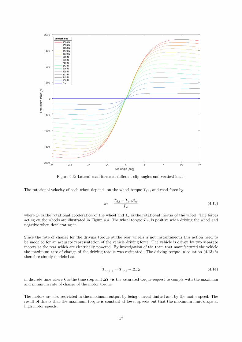
The lateral road force is then estimated by linear 2D-interpolation from the wheel load and slip angles. Figure 4.3illustrates the captured data for the lateral force as a function of the slip angle at varying loads.

4.2.3 Longitudinal tire forces

The non-linear interaction between the tires and ground can be modelled as a function of slip and vertical load.For the tire-road friction force there was no empirical data for the research vehicle available and therefore asemi-empirical model similar to Pacejka’s magic tire formula was used. The longitudinal force was calculatedas

Fx,i = µiFz,i sin(C arctan(Bsx,i − E(Bsx,i − arctan(Bsx,i)))) (4.11)

for i = {FL,Fr,Rl,Rr}. Here µi is the friction coefficient, Fz,i is the tire load, B, C, and E are fittingparameters and sx,i is the longitudinal slip ratio of each tire. The slip is in turn given by

sxi=Rw · ωi − vx

vx(4.12)

where Rw is the radius of the wheel and ωi is the rotational speed of each wheel.

16

-20 -15 -10 -5 0 5 10 15 20

Slip angle [deg]

-2000

-1500

-1000

-500

0

500

1000

1500

2000

Late

ral tire

forc

e [N

]1500 N

1393 N

1286 N

1179 N

1072 N

965 N

858 N

750 N

643 N

536 N

429 N

322 N

215 N

108 N

0 N

Vertical load

Figure 4.3: Lateral road forces at different slip angles and vertical loads.

The rotational velocity of each wheel depends on the wheel torque Td,i, and road force by

ωi =Td,i − Fx,iRw

Iw(4.13)

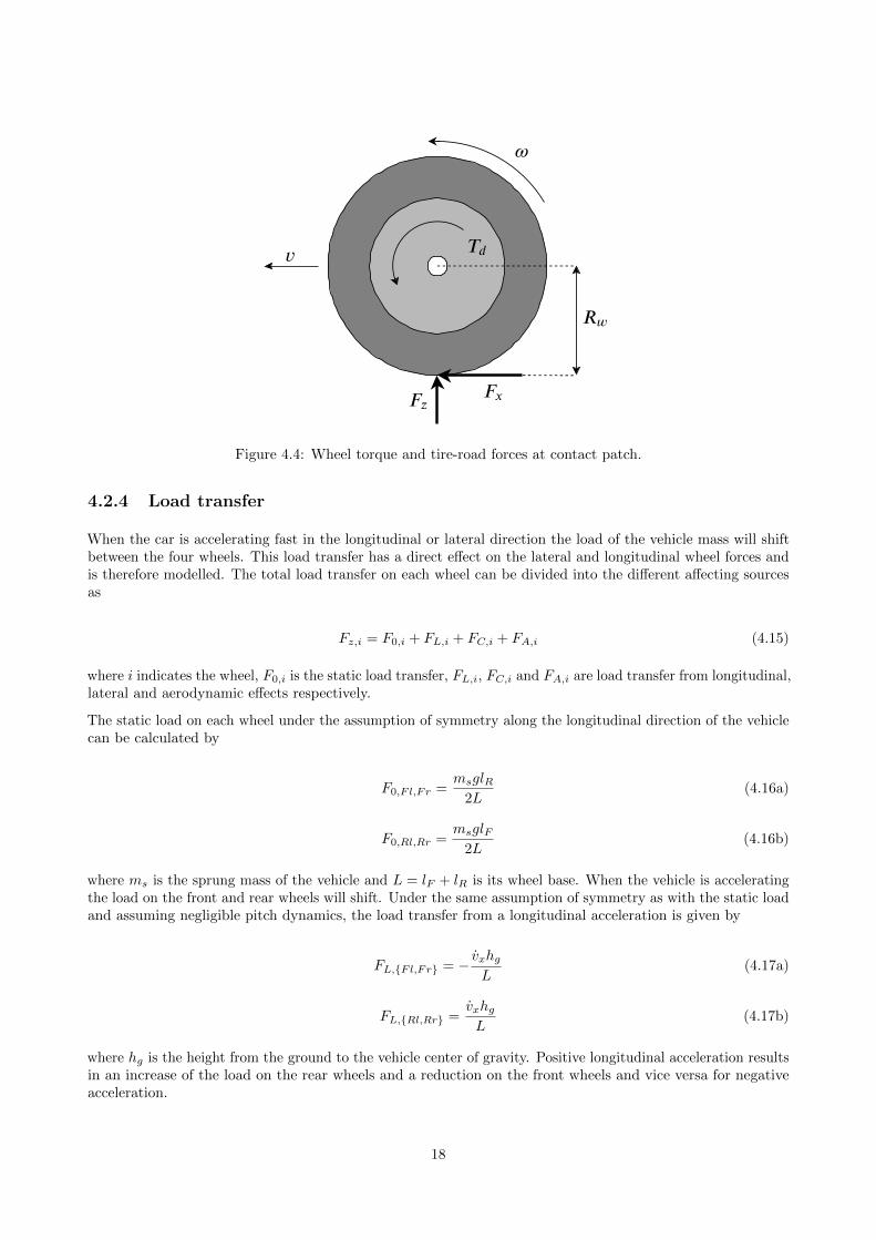
where ωi is the rotational acceleration of the wheel and Iw is the rotational inertia of the wheel. The forcesacting on the wheels are illustrated in Figure 4.4. The wheel torque Td,i is positive when driving the wheel andnegative when decelerating it.

Since the rate of change for the driving torque at the rear wheels is not instantaneous this action need tobe modeled for an accurate representation of the vehicle driving force. The vehicle is driven by two separatemotors at the rear which are electrically powered. By investigation of the team that manufactured the vehiclethe maximum rate of change of the driving torque was estimated. The driving torque in equation (4.13) istherefore simply modeled as

Td,ik+1= Td,ik + ∆Td (4.14)

in discrete time where k is the time step and ∆Td is the saturated torque request to comply with the maximumand minimum rate of change of the motor torque.

The motors are also restricted in the maximum output by being current limited and by the motor speed. Theresult of this is that the maximum torque is constant at lower speeds but that the maximum limit drops athigh motor speeds.

17

��

��

�

��

�

��

��

Figure 4.4: Wheel torque and tire-road forces at contact patch.

4.2.4 Load transfer

When the car is accelerating fast in the longitudinal or lateral direction the load of the vehicle mass will shiftbetween the four wheels. This load transfer has a direct effect on the lateral and longitudinal wheel forces andis therefore modelled. The total load transfer on each wheel can be divided into the different affecting sourcesas

Fz,i = F0,i + FL,i + FC,i + FA,i (4.15)

where i indicates the wheel, F0,i is the static load transfer, FL,i, FC,i and FA,i are load transfer from longitudinal,lateral and aerodynamic effects respectively.

The static load on each wheel under the assumption of symmetry along the longitudinal direction of the vehiclecan be calculated by

F0,F l,Fr =msglR

2L(4.16a)

F0,Rl,Rr =msglF

2L(4.16b)

where ms is the sprung mass of the vehicle and L = lF + lR is its wheel base. When the vehicle is acceleratingthe load on the front and rear wheels will shift. Under the same assumption of symmetry as with the static loadand assuming negligible pitch dynamics, the load transfer from a longitudinal acceleration is given by

FL,{Fl,Fr} = − vxhgL

(4.17a)

FL,{Rl,Rr} =vxhgL

(4.17b)

where hg is the height from the ground to the vehicle center of gravity. Positive longitudinal acceleration resultsin an increase of the load on the rear wheels and a reduction on the front wheels and vice versa for negativeacceleration.

18

For the lateral load the roll dynamics are taken into account in the model under the assumption of steady stateand that the roll angles are small. In steady state the roll angle of the vehicle is given by

cφφ = msvyhφ cos(φ) +msghφ sin(φ) (4.18)

where φ is the roll angle, cφ is the vehicle roll stiffness, hφ is the height difference between the roll axis andcenter of gravity. Since the roll angle is assumed to be small equation (4.18) can be solved as

φ =msvyhφ

cφ −mshφg. (4.19)

By moment equilibrium around the roll axis’ the lateral load transfer is obtained as

FC,{Fl,Fr} =1

2wF(cφ,Fφ+

lRLmsvy) (4.20a)

FC,{Rl,Rr} =1

2wR(cφ,Rφ+

lFLmsvy) (4.20b)

where cφ,F and cφ,R are the effective cornering stiffness at the front or rear roll axles.

Since the vehicle is designed for high speed cornering the aerodynamic packages have a noticeable effect on thelongitudinal load transfer. Assuming all aerodynamic lift and drag forces can be summed up at a single pointwith height hp and longitudinal distance lp the load on each wheel can be calculated as

FA,{Fl,Fr} =1

4LρA(Clv

2x(lR − lp)− Cdhp) (4.21a)

FA,{Rl,Rr} =1

4LρA(Clv

2x(lR + lp) + Cdhp). (4.21b)

4.3 Reference path generation

For the lateral control to work, a local path is needed. This path would be the output of the path plannermodule given as a list of coordinates relative to the car’s local frame. This path is updated at the samefrequency as the lateral controller.

4.3.1 Generating reference path from local path

To use the local path as reference trajectory for the lateral controller, the path needs to be redefined. Assumingif there is an optimal steering angle sequence such that the car could track the local path perfectly, then onecould divide the local path into a number of segments; each segment is the distance covered by the car in onesampling time. Then the first np segments, where np is the prediction horizon for the MPC lateral controller,would be chosen as the reference local path. Figure 4.5 illustrates the path with its segments.

Assume the longitudinal speed of the car, vx, is constant within the prediction horizon. np is the predictionhorizon, np,max is the maximum prediction horizon, Lp is the total local path length, Ts is the sampling time.Then np would be

N = min

(ceil

(LpvxTs

), np,max

)(4.22)

where ceil() would return the nearest rounded integer greater than or equal to the argument.

19

Figure 4.5: Generation of prediction horizon with np segments.

4.4 Longitudinal control

This section provides an insight to how the longitudinal speed of the vehicle is set during simulation and iswhat was implemented on the formula race car and how the decoupled lateral control works together with thelongitudinal control of the vehicle.

The lateral acceleration of the vehicle can be estimated based on the curvature of the road as

vy =v2x

R(4.23)

where vx is the speed of the vehicle and R is represents the path radius at some given part of the track. If thecurvature of the track is known a reference velocity can be calculated based on the vehicles maximum lateralacceleration as

vx =√ay,maxR (4.24)

where vx is the velocity reference at a given point and ay,max is the maximum lateral acceleration. By calculatinga velocity reference for all points in the given local path it is possible to trace back from the last point tothe first to ensure that the maximum longitudinal acceleration is not exceeded. If it is, the velocities arerecalculated with the maximum longitudinal acceleration to ensure that all reference velocities can be reached

20

by the vehicle. Based on these velocities the required acceleration can be calculated by differentiation as

ax,k =vx,k+1 − vx,k

tk(4.25)

where ax,k is the longitudinal acceleration at point k, vk is the reference velocity at point k and tk is the timeit takes to move from point k to k + 1. The time between points, tk is estimated as

tk =2sk

vx,k+1 + vx,k(4.26)

where sk is the Euclidean distance between point k and k + 1.

This acceleration is then used to calculate the force to accelerate the vehicle

Fx,k = m(vx,k + gfr) +1

2CdAρv

2x,k (4.27)

where mvx,k is the inertial force to accelerate the vehicle, mgfr is the approximated roll resistance of the wheelsand 1

2CdAρv2x,k is the air resistance with Cd being the drag coefficient, A being the frontal area of the vehicle

and ρ being the air density. The required motor torque can then be calculated as

Tm,k =Fx,kRwK

(4.28)

where Tm is the motor torque, Rw is the wheel radius and K is the gear ratio.

4.5 Lateral control

Two models for lateral control were investigated for the control model: a kinematic model, and a dynamic model.The kinematic model is simple and therefore not computationally demanding for the controller. However, itdoes not model the vehicle state change at higher velocities as well as compared to the dynamic model. Thereis therefore a trade off between the accuracy of the vehicle model for the controller and the computationaleffort. An addition is made to the dynamic model to include the vehicle motor differentials to enable torquevectoring.

4.5.1 Kinematic model

A simple kinematic model is used as the lateral controller model, with three states: the car’s coordinate in

Cartesian coordinate system and the heading x =[x, y, θ

]T; and one control input: the steering angle u =

[δ].

The assumption for choosing this model is that the car does not run at sufficiently high speed while takingcurves, so that the lateral forces and side slips are small. The state evolution equations are

x = vx cos θ (4.29)

y = vx cos θ (4.30)

θ = vxtan(δ)

L(4.31)

21

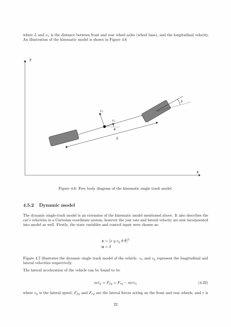
where L and vx is the distance between front and rear wheel axles (wheel base), and the longitudinal velocity.An illustration of the kinematic model is shown in Figure 4.6

�

�

��

�

�

�

��

Figure 4.6: Free body diagram of the kinematic single track model.

4.5.2 Dynamic model

The dynamic single-track model is an extension of the kinematic model mentioned above. It also describes thecar’s velocities in a Cartesian coordinate system, however the yaw rate and lateral velocity are now incorporatedinto model as well. Firstly, the state variables and control input were chosen as:

x = [x y vy θ θ]T

u = δ

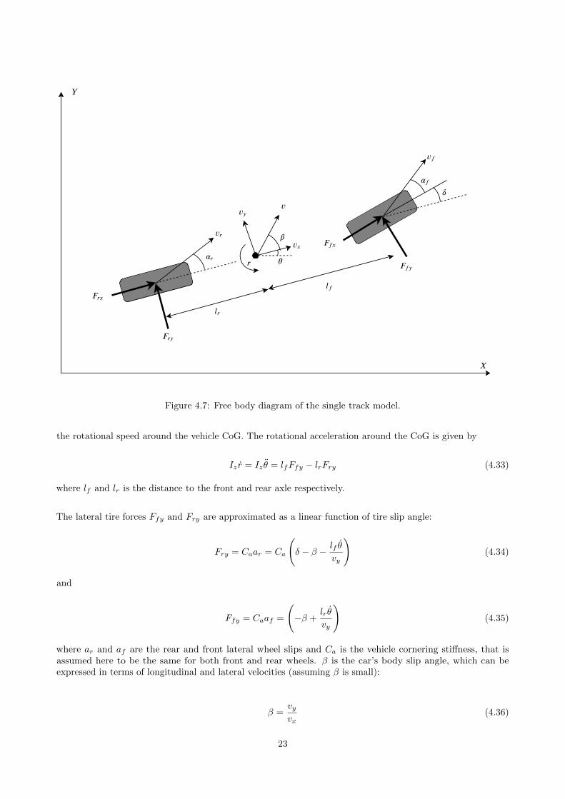
Figure 4.7 illustrates the dynamic single track model of the vehicle. vx and vy represent the longitudinal andlateral velocities respectively.

The lateral acceleration of the vehicle can be found to be

mvy = Ffy + Fry −mrvx (4.32)

where vy is the lateral speed, Ffy and Fry are the lateral forces acting on the front and rear wheels, and r is

22

�

�

�

��

��

�

���

���

��

��

���

�

��

��

���

��

��

�

�

Figure 4.7: Free body diagram of the single track model.

the rotational speed around the vehicle CoG. The rotational acceleration around the CoG is given by

Iz r = Iz θ = lfFfy − lrFry (4.33)

where lf and lr is the distance to the front and rear axle respectively.

The lateral tire forces Ffy and Fry are approximated as a linear function of tire slip angle:

Fry = Caar = Ca

(δ − β − lf θ

vy

)(4.34)

and

Ffy = Caaf =

(−β +

lr θ

vy

)(4.35)

where ar and af are the rear and front lateral wheel slips and Ca is the vehicle cornering stiffness, that isassumed here to be the same for both front and rear wheels. β is the car’s body slip angle, which can beexpressed in terms of longitudinal and lateral velocities (assuming β is small):

β =vyvx

(4.36)

23

Combining the above three equation gives:

Fry = Ca

(δ − vy

vx− lf θ

vy

)(4.37)

Ffy =

(−vyvx

+lr θ

vy

)(4.38)

States of interest are vy and θ which can be given by:

• Substituting 4.37 into 4.33 and 4.32.

• Expressing vy and θ as functions of other state variables and control input

This would give

vy =

(−2Cavxm

)vy +

(−vx −

Ca(lf + lr)

vxm

)θ +

(Cam

)δ (4.39)

θ =

(Ca(lr − lf )

Izvx

)vy +

(−Ca(l2f + l2r)

vxm

)θ +

(lfCaIz

)δ (4.40)

and vy, θ and θ can be found by integrating vy and θ.The change of position of the car in the inertial frame is given by

X = vx cos(θ)− vy sin(θ) (4.41)

andY = vx sin(θ) + vy cos(θ). (4.42)

Equation 4.39, 4.40, 4.41, and 4.42 describe the state evolution of the dynamic model.

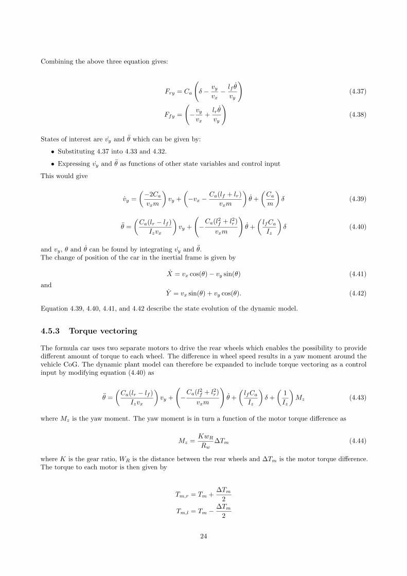
4.5.3 Torque vectoring

The formula car uses two separate motors to drive the rear wheels which enables the possibility to providedifferent amount of torque to each wheel. The difference in wheel speed results in a yaw moment around thevehicle CoG. The dynamic plant model can therefore be expanded to include torque vectoring as a controlinput by modifying equation (4.40) as

θ =

(Ca(lr − lf )

Izvx

)vy +

(−Ca(l2f + l2r)

vxm

)θ +

(lfCaIz

)δ +

(1

Iz

)Mz (4.43)

where Mz is the yaw moment. The yaw moment is in turn a function of the motor torque difference as

Mz =KwRRw

∆Tm (4.44)

where K is the gear ratio, WR is the distance between the rear wheels and ∆Tm is the motor torque difference.The torque to each motor is then given by

Tm,r = Tm +∆Tm

2

Tm,l = Tm −∆Tm

2

24

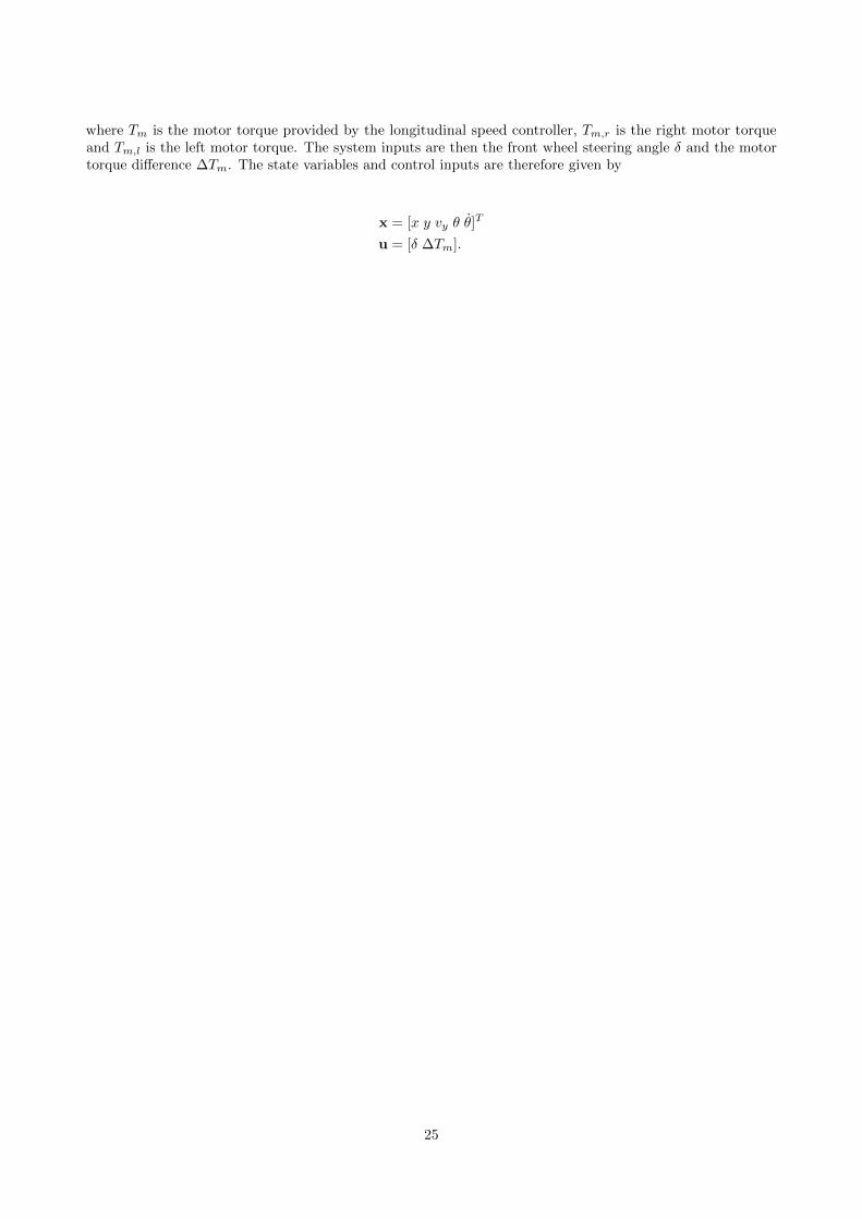
where Tm is the motor torque provided by the longitudinal speed controller, Tm,r is the right motor torqueand Tm,l is the left motor torque. The system inputs are then the front wheel steering angle δ and the motortorque difference ∆Tm. The state variables and control inputs are therefore given by

x = [x y vy θ θ]T

u = [δ ∆Tm].

25

5 Results

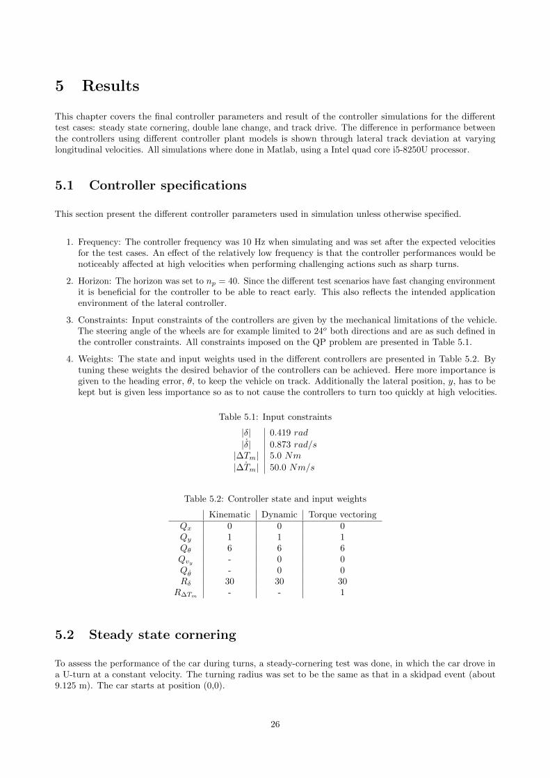
This chapter covers the final controller parameters and result of the controller simulations for the differenttest cases: steady state cornering, double lane change, and track drive. The difference in performance betweenthe controllers using different controller plant models is shown through lateral track deviation at varyinglongitudinal velocities. All simulations where done in Matlab, using a Intel quad core i5-8250U processor.

5.1 Controller specifications

This section present the different controller parameters used in simulation unless otherwise specified.

1. Frequency: The controller frequency was 10 Hz when simulating and was set after the expected velocitiesfor the test cases. An effect of the relatively low frequency is that the controller performances would benoticeably affected at high velocities when performing challenging actions such as sharp turns.

2. Horizon: The horizon was set to np = 40. Since the different test scenarios have fast changing environmentit is beneficial for the controller to be able to react early. This also reflects the intended applicationenvironment of the lateral controller.

3. Constraints: Input constraints of the controllers are given by the mechanical limitations of the vehicle.The steering angle of the wheels are for example limited to 24o both directions and are as such defined inthe controller constraints. All constraints imposed on the QP problem are presented in Table 5.1.

4. Weights: The state and input weights used in the different controllers are presented in Table 5.2. Bytuning these weights the desired behavior of the controllers can be achieved. Here more importance isgiven to the heading error, θ, to keep the vehicle on track. Additionally the lateral position, y, has to bekept but is given less importance so as to not cause the controllers to turn too quickly at high velocities.

Table 5.1: Input constraints

|δ| 0.419 rad

|δ| 0.873 rad/s|∆Tm| 5.0 Nm

| ˙∆Tm| 50.0 Nm/s

Table 5.2: Controller state and input weights

Kinematic Dynamic Torque vectoringQx 0 0 0Qy 1 1 1Qθ 6 6 6Qvy - 0 0Qθ - 0 0Rδ 30 30 30

R∆Tm - - 1

5.2 Steady state cornering

To assess the performance of the car during turns, a steady-cornering test was done, in which the car drove ina U-turn at a constant velocity. The turning radius was set to be the same as that in a skidpad event (about9.125 m). The car starts at position (0,0).

26

After several runs, it was found that the maximum velocity that the car could make the turn without hittingany cone is 40 km/h. Any velocity higher than this would result in driving off the track. Figure 5.1 shows theposition trace of the car using the dynamic model (with and without torque vectoring) and kinematic modelfor lateral controller. In general, all three models behaved similarly. Nevertheless, there is a slight difference:the dynamic models were slightly more under steering, compared to the kinematic model.

-15 -10 -5 0 5 10 15 20 25 30

x (m)

0

5

10

15

20

25

30

35

40

y (

m)

Position of car for u turn using different models

dynamic

dynamic-torque

kinematic

blue cones

yellow cones

Figure 5.1: U-turn with position of the car using different lateral controller models.

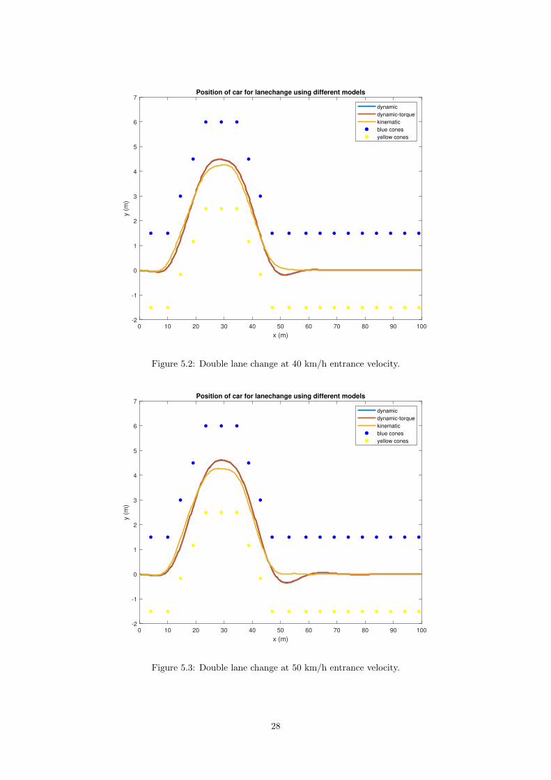
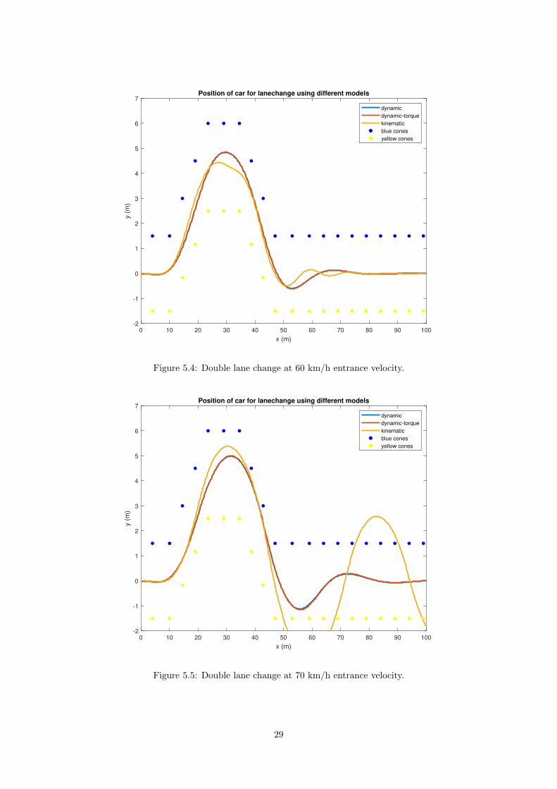
5.3 Double lane change

Figure 5.2–5.5 illustrate the position traces of the car using different models of controller, for the double lanechange test case. Due to the constant-speed assumption while designing the controller, the lane change testwere done with four different constant speeds: 40, 50, 60 and 70 km/h.

From the four speed settings, it can be seen that at low speeds (40 and 50 km/h), all controller models couldhandle well, albeit the kinematic model performs slightly better. However, at higher speed (70 and 80 km/h),the dynamic models (both with and without torque vectoring) are more stable: at 70 km/h, the maximumlateral deviation is about 0.3 m for all models, but the kinematic model started to exhibit oscillatory behaviour.At 80 km/h, both dynamic models can still keep the car follow the lane, albeit with larger lateral deviation,whereas the kinematic model completely drove the car outside the lane with large, oscillatory lateral error. Athigher velocities than 80 km/h, no model could keep the car in lane.The controller frequency also has noticeable impact on the steering performance. A similar test for lanechanging at 70km/h for all three controller models was also run, but now the controller was set to run at 50 Hz.It was observed that at 50 Hz, the dynamic models (both with and without torque vectoring) performed betterthan at 10 Hz, the difference can be seen when the car reaches the 60 m mark, where the deviation from pathcenterline was 1.3 m at 10 Hz, and 0.4 m at 50 Hz,a 70 percent reduction in lateral deviation. For the kinematic

27

0 10 20 30 40 50 60 70 80 90 100

x (m)

-2

-1

0

1

2

3

4

5

6

7

y (

m)

Position of car for lanechange using different models

dynamic

dynamic-torque

kinematic

blue cones

yellow cones

Figure 5.2: Double lane change at 40 km/h entrance velocity.

0 10 20 30 40 50 60 70 80 90 100

x (m)

-2

-1

0

1

2

3

4

5

6

7

y (

m)

Position of car for lanechange using different models

dynamic

dynamic-torque

kinematic

blue cones

yellow cones

Figure 5.3: Double lane change at 50 km/h entrance velocity.

28

0 10 20 30 40 50 60 70 80 90 100

x (m)

-2

-1

0

1

2

3

4

5

6

7

y (

m)

Position of car for lanechange using different models

dynamic

dynamic-torque

kinematic

blue cones

yellow cones

Figure 5.4: Double lane change at 60 km/h entrance velocity.

0 10 20 30 40 50 60 70 80 90 100

x (m)

-2

-1

0

1

2

3

4

5

6

7

y (

m)

Position of car for lanechange using different models

dynamic

dynamic-torque

kinematic

blue cones

yellow cones

Figure 5.5: Double lane change at 70 km/h entrance velocity.

29

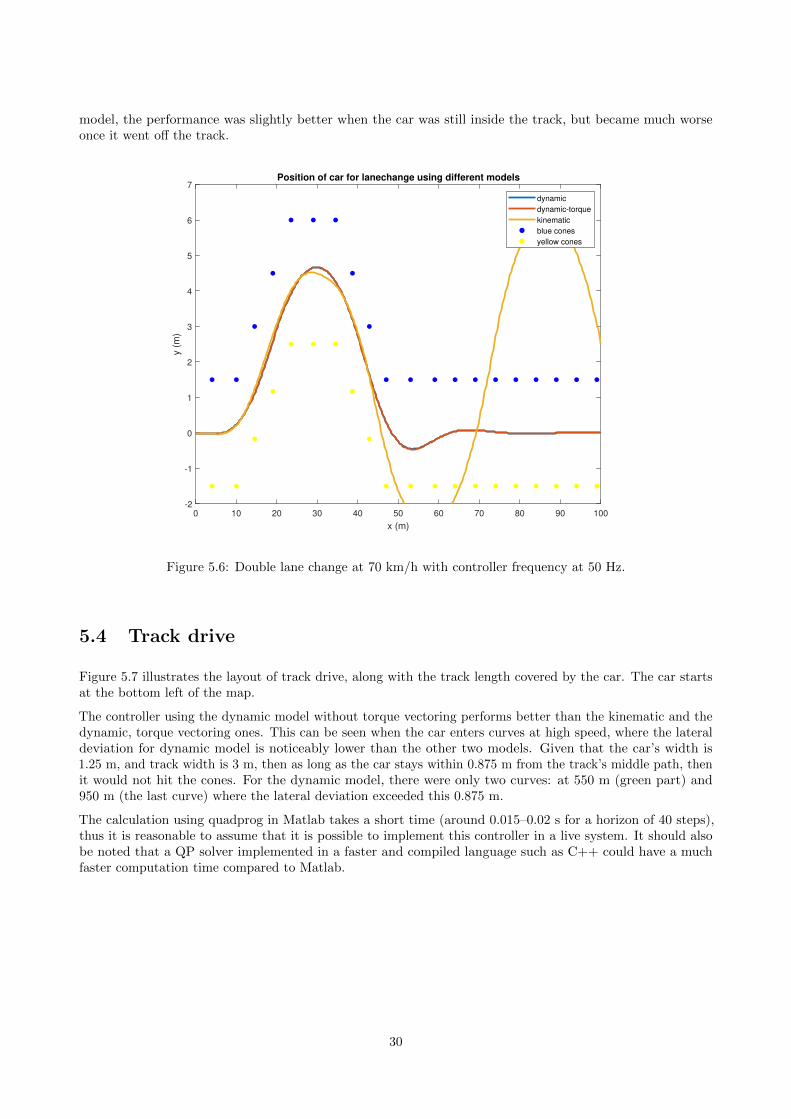
model, the performance was slightly better when the car was still inside the track, but became much worseonce it went off the track.

0 10 20 30 40 50 60 70 80 90 100

x (m)

-2

-1

0

1

2

3

4

5

6

7

y (

m)

Position of car for lanechange using different models

dynamic

dynamic-torque

kinematic

blue cones

yellow cones

Figure 5.6: Double lane change at 70 km/h with controller frequency at 50 Hz.

5.4 Track drive

Figure 5.7 illustrates the layout of track drive, along with the track length covered by the car. The car startsat the bottom left of the map.

The controller using the dynamic model without torque vectoring performs better than the kinematic and thedynamic, torque vectoring ones. This can be seen when the car enters curves at high speed, where the lateraldeviation for dynamic model is noticeably lower than the other two models. Given that the car’s width is1.25 m, and track width is 3 m, then as long as the car stays within 0.875 m from the track’s middle path, thenit would not hit the cones. For the dynamic model, there were only two curves: at 550 m (green part) and950 m (the last curve) where the lateral deviation exceeded this 0.875 m.

The calculation using quadprog in Matlab takes a short time (around 0.015–0.02 s for a horizon of 40 steps),thus it is reasonable to assume that it is possible to implement this controller in a live system. It should alsobe noted that a QP solver implemented in a faster and compiled language such as C++ could have a muchfaster computation time compared to Matlab.

30

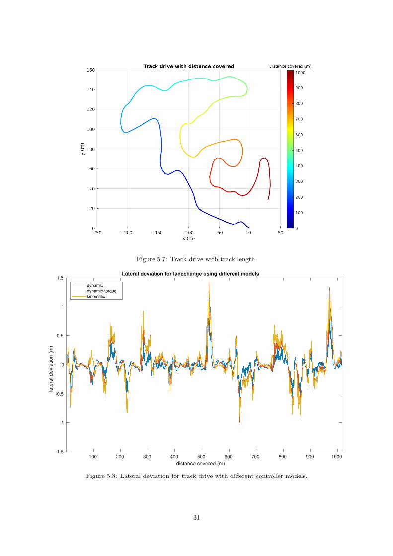
Figure 5.7: Track drive with track length.

100 200 300 400 500 600 700 800 900 1000

distance covered (m)

-1.5

-1

-0.5

0

0.5

1

1.5

late

ral d

evia

tion

(m

)

Lateral deviation for lanechange using different models

dynamic

dynamic-torque

kinematic

Figure 5.8: Lateral deviation for track drive with different controller models.

31

Figure 5.9: Longitudinal velocity for track drive with different controller models. All controller models resultedin nearly identical velocity profiles.

32

6 Discussion

In this thesis the design and implementation of linear time variant model predictive steering controllers havebeen presented together with the simulated result with a given vehicle model. Two different control models wereused: a kinematic pointmass model, and a dynamic single track model with decoupled longitudinal and lateraldynamics. The different lateral controllers were tested in three test scenarios: a steady state cornering test, adouble lane change test, and a track drive test suing the track layout of Formula Student Germany. The resultsof using different controller models have also been presented and a comparison between their performances canbe made.

In steady state cornering test, the car drives in a u-turn with a constant turning radius at constant speed. Thistest will reveal a vehicle’s oversteering and understeering properties. From the test results, it shows that thekinematic model controller appears to be more responsive than the dynamic model controllers in steady-stateconditions. This could be due to the reactive nature of the kinematic model, where a control input is calcu-lated directly from the local path information, without taking into account the dynamic properties of the vehicle.

In double lane change test, the car will perform two lane-change maneuver while trying to stay as close tothe lane centerline as possible. These maneuvers are commonly used to test the vehicle’s ability in handlinghigh dynamic situations. The test results show that in high dynamic situations, the dynamic model controllersperform better than the kinematic controller, especially at high speeds. In addition, the controllers were alsotested at two different frequencies (10 Hz and 50 Hz) at 70 km/h longitudinal speed, and as expected thelateral control performance was much better at the higher frequency: the car managed to stay 70 percent closerto the lane centerline, and the increased controller frequency did not result in any significant computationaltime increase.

Lastly, a track drive test was carried out for all three controllers, to assess their performance in an openenvironment. In this test a full racing lap simulation was done, where the car would drive through a racing track.The track is composed of straight lines, constant radius turns, hairpin turns. This combination of differentmaneuvers will test the overall performances of the controllers. Lateral deviation from the track centerline wasrecorded for all controllers, in order to judge their lateral control performance. A speed profile along the trackof all controllers was also recorded, to judge the longitudinal controller performance. From 5.8, it shows thatthe lateral controllers are good enough to keep the car inside the track most of the time, there are only twoplaces where the lateral deviation are higher than 0.8 meter which were considered to be outside of the safezone. These places correspond to two sharp turns after a straight line, where the car has to slow down fast totake the turn. As the longitudinal speed has to change quickly, the lateral controllers which assumed a constantlongitudinal speed in the dynamic model, would become less accurate, and thus results in a poor performance.The longitudinal speed profile shows that the top speed reached was only 63 km/h, a rather slow speed forracing car. Nevertheless, this speed is acceptable, as it is easier to keep the car stay within the 3 meter wide track.

Using Matlab’s quadratic programming solver quadprog the mean execution times on a Intel quad corei5-8250U are around 4 ms for all controllers. This provides a good indication that the controller designs wouldhave feasible execution times if implemented in the real world on the formula car. If the controller wouldbe implemented on the formula car it would also be written in a compiled language such as C++ whichmight improve the execution time further. However, the MPC controller would also run alongside many otherprograms on the vehicle and as such it is not possible to make any estimation on the execution time of theproposed controller designs on the real system.

From the results it is apparent that the different controller performance are similar. In the case of the U-turnthe different controllers can keep the vehicle close enough to the center line at roughly the same maximumlongitudinal speed. The only noticeable difference is that the dynamic models were understeering more whencompared to the kinematic model. The understeering of the dynamic model controller could be cased byinaccuracies in the lateral and rotational dynamics of the control model. In the double lane change test thecontroller performances were once again similar at lower speeds. At higher speeds however, the kinematic

33

controller loses control of the vehicle completely. This test shows a clear difference between the controllers athigher longitudinal speed indicates that the dynamic model controller might be preferable in the actual vehicle.During the track drive the dynamic based controller generally performs better in keeping the vehicle close tothe track centerline. The difference during sharp turns is also large enough to possibly make the differencebetween hitting a cone or not during competition.

From the controller performances there is a minor difference between the controllers based on the kinematic anddynamic models while the calculation time remains roughly the same. The controller using the kinematic modelwould appear to be sufficient at lower longitudinal speeds but, as could be seen in the double lane change test, itperforms worse at higher longitudinal and lateral speeds. The dynamic model controller also generally performsbetter at the track drive where the longitudinal speed is constantly changing. Since the calculation time isalso the same between models, the dynamic model based controller might be favourable to use in the real vehicle.

Since the proposed lateral controllers are decoupled from the longitudinal control they perform better at constantspeed. Cornering performance is worsened since the speed is assumed to be constant during linearization of thecontroller plant model while it is changing during simulation. This can be seen during the track drive testing inresults where the vehicle slows down when approaching a turn which leads to worsened lateral performance. Bet-ter performance could be achieved if the change in speed is taken into account when planning the steering actionof the vehicle. However, literature study about performance of coupled and decoupled steering control has beenmentioned, which showed that the a coupled dynamic model will have higher complexity and thus is harder totune, while the performance improvement is little. In addition, the increased complexity will also result in longerexecution time of the controller. From the double lane change test result, it can be seen that much better steeringperformance can be achieved with only a decoupled model but at higher frequency (50 Hz instead of 10 Hz). Thus,it can be concluded that the decoupled MPC steering controller has performed well in this specified environment.

The weight matrices Q (state weights) and R (control input weights) were carefully tuned during each testscenario to maximize the performance. For all tests, the weights were chosen as (Qx, Qy, Qvy , Qθ, Qθ) = (0,

1, 6, 0, 0) for Q, and (θ) = (30) for R (where x, y are the car position, vy is lateral velocity, θ is yaw rate of

the car, and θ is the steer angle rate in radians per second, all are in the car’s local frame). It could be seenthat the lateral velocity has a big impact on the steering performance amongst all states; the steering rateweight does not have a big impact because it was in radians and not degree. Tuning the weights require a lotof trials, and one has to account for how each state affects another. The tuning strategy was as follow: first setall weights to zero, then increase the control input weight until the car could somehow follow the track, thenincrease the state weights, on by one, until the desired performance is obtained. As mentioned before, tuningrequires a lot of trials and depends a lot on the actual dynamic of the system. This set of weights was the mostoptimized, and further tuning did not result in any performance improvement.

With the proposed controller designs the steering angle and steering rate are kept at all times. This providesa way to take the constraints of the physical system into account when planning the steering action of thevehicle. Due to the physical limitations of the steering system on the vehicle the steering rate is low and thus itis beneficial to take into account in the controller.

In the controllers, Cartesian coordinates were used to represent the local path. Since the local path is thecenter line of the tracks, a curvilinear coordinate system might have provided a better representation of thesystem since it would have been possible to represent the change in curvature in the model. In the currentsystem representation the model does not take the turn rate of the path into account when modeling the vehicledynamics which could possibly have a noticeable effect on the controller performances. With a curvilinearcoordinate system and using the path deviation as a state it would also be possible to add constraints on thepath deviation in the controller design. One could additionally explore the use of constraints on system statessuch as lateral acceleration and yaw rate.

34

7 Conclusions

Satisfactory steering behavior could be achieved in simulation for decoupled lateral control using MPC. Allthree controllers performed well in the different test cases at lower velocities and could be considered for testingin the real world on the formula car. While the different controllers performed similarly, using a dynamicvehicle model had slightly better performance at higher velocities. The controller utilizing a kinematic vehiclemodel did perform better at the cornering test due to less understeering. However, since the controllers usinga dynamic model did perform better overall while not increasing the computational complexity by much, itshould be considered firsthand if tested on the real car.

It can be concluded that the controllers all performed sufficiently within the simulation environment and couldbe considered for testing on the real vehicle. A difference in the performance of the kinematic and dynamicbased controllers could be observed in simulation. It is however not possible to make any conclusions on theiractual performance in the real vehicle due to the limitations of the simulation environment.

7.1 Future work

The proposed controllers all have acceptable performance at somewhat high speeds. There are however aspectsto the controllers that could be investigated for further improvements. A possibility would be to investigatecoupled longitudinal and lateral control to provide insight to the benefits of coupled control in the applicationenvironment. One could also change the path representation to a curvilinear coordinate system which wouldprovide the possibility to constrain the path deviation in the MPC formulation. With coupled longitudinal andlateral control this could improve the car’s ability to stay on track during sharp turns.

No verification data of the vehicle movement could be collected during this work which would have providedbetter insight on the performance of the controller on the actual formula car. As it stands right now nothingcan be said about the performance of the designed controllers outside of the simulation environment.

Very little can be said about the controller execution time outside of the simulation environment in Matlab.A formal analysis of the execution time to verify real-time capabilities of the controller could additionally bedone. To implement the controllers on the formula car the current controller code would have to be ported tocode that can run in the formula car execution environment. This would most likely also serve to improve theexecution time of the MPC calculations.

35

References

[1] F. S. Germany. An outlook on FSG 2021 and the following seasons. 2018. url: https://n.fs-g.org/1064(visited on 12/28/2018).

[2] E. F. Camacho and C. B. Alba. Model Predictive Control. 2nd ed. 1-29. Springer Verlag, 2004. isbn:9780857293985.

[3] S. Qin and T. A. Badgwell. A survey of industrial model predictive control technology. Control EngineeringPractice 11.7 (2003), 733–764. issn: 0967-0661. doi: https://doi.org/10.1016/S0967-0661(02)00186-7. url: http://www.sciencedirect.com/science/article/pii/S0967066102001867.

[4] M. Zanon et al. “Model Predictive Control of Autonomous Vehicles”. Vol. 455. Mar. 2014. doi: 10.1007/978-3-319-05371-4_3.

[5] R. Verschueren et al. “Towards time-optimal race car driving using nonlinear MPC in real-time”. 53rdIEEE Conference on Decision and Control. 2014, pp. 2505–2510. doi: 10.1109/CDC.2014.7039771.

[6] Y. Yoon et al. Model-predictive active steering and obstacle avoidance for autonomous ground vehicles.Control Engineering Practice 17 (July 2009), 741–750. doi: 10.1016/j.conengprac.2008.12.001.

[7] P. Falcone et al. Predictive Active Steering Control for Autonomous Vehicle Systems. Control SystemsTechnology, IEEE Transactions on 15 (June 2007), 566–580. doi: 10.1109/TCST.2007.894653.

[8] J. Kong et al. “Kinematic and dynamic vehicle models for autonomous driving control design”. 2015IEEE Intelligent Vehicles Symposium (IV). June 2015, pp. 1094–1099. doi: 10.1109/IVS.2015.7225830.

[9] K. Lundahl, J. Aslund, and L. Nielsen. Investigating Vehicle Model Detail for Close to Limit ManeuversAiming at Optimal Control (May 2012).

[10] R. Attia, R. Orjuela, and M. Basset. “Coupled longitudinal and lateral control strategy improving lateralstability for autonomous vehicle”. 2012 American Control Conference (ACC). June 2012, pp. 6509–6514.doi: 10.1109/ACC.2012.6315130.

[11] R. Attia, R. Orjuela, and M. Basset. Combined longitudinal and lateral control for automated vehicleguidance. Vehicle System Dynamics: International Journal of Vehicle Mechanics and Mobility 52 (Jan.2014), 261–279. doi: 10.1080/00423114.2013.874563.

[12] C. Olsson. “Model Complexity and Coupling of Longitudinal and Lateral Control in Autonomous VehiclesUsing Model Predictive Control”. PhD thesis. May 2015. url: http://urn.kb.se/resolve?urn=urn:nbn:se:kth:diva-175389.

[13] P. Falcone et al. “A linear time varying model predictive control approach to the integrated vehicledynamics control problem in autonomous systems”. 2007 46th IEEE Conference on Decision and Control.Dec. 2007, pp. 2980–2985. doi: 10.1109/CDC.2007.4434137.

[14] A. Katriniok and D. Abel. LTV-MPC approach for lateral vehicle guidance by front steering at thelimits of vehicle dynamics. In Proceedings of the IEEE Decision and Control and IEEE European ControlConference 52 (2011), 6828–6833.

[15] A. Zhakatayev et al. Successive linearization based model predictive control of variable stiffness actuatedrobots (July 2017), 1774–1779. issn: 2159-6255. doi: 10.1109/AIM.2017.8014275.

[16] H. Zheng. Trajectory Tracking of Autonomous Vessels Using Model Predictive Control (Aug. 2014),8812–8818. doi: 10.3182/20140824-6-ZA-1003.00767.

36

[17] A. Karlsson. Test Procedures and Evaluation Tools for Passenger Vehicle Dynamics (2014).

37