use of individual wheel steering to improve vehicle
TRANSCRIPT

Use of individual wheel steering to improve vehicle stability and disturbance rejection
by
Richard C.K. Nkhoma
Submitted in partial fulfilment of the requirements for the degree
MSc (Applied Science) Mechanical
in the Faculty of
Engineering, Built Environment and Information Technology
University of Pretoria, Pretoria
October 2009
©© UUnniivveerrssiittyy ooff PPrreettoorriiaa
Abstract
i
Use of individual wheel steering to improve vehicle stability
and disturbance rejection
By
Richard C.K. Nkhoma
Supervisor : Prof. N.J. Theron
Department : Mechanical and Aeronautical Engineering
Degree : MSc (Applied Science) Mechanical
ABSTRACT
The main aim of this research project is to extend theories of four-wheel-steering as
developed by J. Ackermann to include an individually steered four-wheel steering system
for passenger vehicles. Ackermann’s theories, including theories available in this subject
area, dwell much on vehicle system dynamics developed from what is called single track
model and some call it a bicycle model. In the bicycle model, the front two wheels are
bundled together. Similarly, the rear wheels are bundled together. The problem with this
is that it assumes two front wheels or two rear wheels to be under the same road, vehicle
and operating conditions. The reality on the ground and experiments that are conducted
are to the contrary. Therefore this study discusses vehicle disturbance rejection through
robust decoupling of yaw and lateral motions of the passenger vehicle.
A mathematical model was developed and simulated using Matlab R2008b. The model
was developed in such a way that conditions can be easily changed and simulated. The

Abstract
ii
model responded well to variations in road and vehicle conditions. Focus was in the
ability of the vehicle to reject external disturbances. To generate yaw moment during
braking, the brake on the left front wheel was disconnected. This was done because
lateral wind generators, as used by Ackermann, were not available. The results from both
simulations and experiments show disturbance rejection in the steady state.
Keywords – Disturbance rejection, yaw rate, lateral acceleration, four wheel steering
(4WS), individual wheel steering (IWS), robust control, robust decoupling.

Acknowledgement
iii
ACKNOWLEDGEMENT I would like to thank, Prof N. J. Theron, who not only served as my supervisor but also
encouraged and challenged me throughout my academic program and whose tireless
efforts and his ever present helping hand made this work a success. I would also like to
thank Prof. S. Els for his invaluable comments and inputs, and not forgetting my office
mate and now Dr. Michael Thoreson who tried all he could to supply solutions to all my
academic questions.
To my wife Catherine and child Peace for their encouragement and love despite the long
distance that separated us. You were a source of inspiration to me in times when the chips
were down.
To all friends too many to mention, I just want to say that thank you for all the moral
support that you rendered to me during my study, particularly I would like to thank
Jimmy Mokhafera for his support during the whole period of my research. May the Good
LORD richly bless you all.
Above all, I would like to thank God through Jesus Christ for HIS mercies and grace
towards me throughout my stay in South Africa.

Table of Contents
iv
TABLE OF CONTENTS
ABSTRACT ........................................................................................................................ i
ACKNOWLEDGEMENT ............................................................................................... iii
TABLE OF CONTENTS ................................................................................................ iv
LIST OF FIGURES ........................................................................................................ vii
LIST OF TABLES ........................................................................................................... ix
NOMENCLATURE ...........................................................................................................x
1 INTRODUCTION......................................................................................................1
1.1 Background ..........................................................................................................1
1.2 Statement of the Problem .....................................................................................2
1.3 Approach ..............................................................................................................2
2 LITERATURE REVIEW .........................................................................................4
2.1 Experimental Vehicle Status ................................................................................4
2.2 Current Research Situation ..................................................................................4
2.2.1 Decoupling controller ......................................................................................4
2.2.2 Drive by wire ...................................................................................................5
2.2.3 Driver assisted control .....................................................................................6
2.2.4 Adaptive Steering Controller ...........................................................................6
2.2.5 2H / H synthesis ..........................................................................................7
2.3 Closing .................................................................................................................9
3 MATHEMATICAL MODELLING .......................................................................10
3.1 Introduction ........................................................................................................10
3.2 Assumptions .......................................................................................................11
3.3 Nonlinear vehicle model equations of motion ...................................................12
3.4 Sideslip angles ...................................................................................................16

Table of Contents
v
3.5 Lateral forces .....................................................................................................18
3.6 Linearized model ...............................................................................................18
3.6.1 Linearized wheel sideslip angles ...................................................................18
3.6.2 Linearized cornering and lateral forces ..........................................................19
3.6.3 Linearized yaw moments ...............................................................................19
3.6.4 Linearized equation of motion .......................................................................20
3.7 Robust controller ................................................................................................22
3.8 The decoupled yaw subsystem...........................................................................26
3.9 Transfer functions ..............................................................................................28
3.9.1 Uncontrolled vehicle system ..........................................................................28
3.9.2 Controlled vehicle system ..............................................................................32
3.10 Position of centre of pressure .............................................................................36
3.11 Conclusion .........................................................................................................38
4 SIMULATIONS AND RESULTS ..........................................................................39
4.1 Decoupled car ....................................................................................................39
4.2 Conventional car ................................................................................................40
4.3 Results ................................................................................................................42
4.3.1 Validation of the model .................................................................................42
4.3.2 Simulations of a conventional and a decoupled vehicle ................................44
4.3.3 New control laws ...........................................................................................47
4.3.4 Simulations of different coefficient of friction .........................................50
5 IMPLEMENTATION OF INDIVIDUAL WHEEL STEERING .......................52
5.1 Introduction ........................................................................................................52
5.2 Motor characterisation .......................................................................................53
5.3 Potentiometer characterisation ...........................................................................57
5.4 DC motor controller ...........................................................................................61

Table of Contents
vi
5.5 Actuator assembly ..............................................................................................65
6 EXPERIMENTAL SETUP .....................................................................................68
6.1 Experimental Results .........................................................................................70
6.1.1 No input from the steering wheel...................................................................70
6.1.2 Sinusoidal input from the steering wheel .......................................................74
7 CONCLUSIONS AND FUTURE WORK .............................................................78
REFERENCES .................................................................................................................81
APPENDIX .......................................................................................................................85

List of Figures
vii
LIST OF FIGURES
Figure 1-1: SAE Vehicle axis system notations (SAE J670e (1976)) ........................... 3
Figure 3-1: Wheels turning the same direction ............................................................ 11
Figure 3-2: Sketch showing wheel sideslip angles ...................................................... 16
Figure 3-3: Decoupling point ....................................................................................... 22
Figure 3-4: Location of centre of pressure ................................................................... 37
Figure 4-1: Actuator model .......................................................................................... 41
Figure 4-2: simulation results at 50 1v m s ......................................................... 43
Figure 4-3: Conventional vehicle with front wheels steering only .............................. 44
Figure 4-4: Robustly decoupled vehicle with front wheel steering only ..................... 45
Figure 4-5: Front wheel steering and individual rear wheel steering .......................... 45
Figure 4-6: Force input response to different ......................................................... 47
Figure 5-1: Experimental vehicle ................................................................................ 53
Figure 5-2: Wiper motor sketch ................................................................................... 54
Figure 5-3: Motor tests setup ...................................................................................... 55
Figure 5-4: Motor response to a step input .................................................................. 55
Figure 5-5: Potentiometer connection sketch .............................................................. 58
Figure 5-6: Actuator unit ............................................................................................. 58
Figure 5-7: Graph of potentiometer angle against potentiometer volts ....................... 60
Figure 5-8: Graph of wheel angle against Potentiometer volts ................................... 61
Figure 5-9: Actuator block diagram. ............................................................................ 62
Figure 5-10: DC Motor Controller circuit diagram ....................................................... 63
Figure 5-11: DC motor Controller circuit box ............................................................... 63
Figure 5-12: Pulse Width Modulation, National Semiconductors (2005) ..................... 64
Figure 5-13: LMD18200 chip, National Semiconductors (2005) .................................. 64
Figure 5-14: LMD18200 circuit diagram, National Semiconductors (2005) ................ 65
Figure 5-15: Actuator – hub assembly connection ........................................................ 66
Figure 5-16: Actuator exploded view ............................................................................ 67
Figure 6-1: A sketch of experimental setup ................................................................. 68
Figure 6-2: Computer................................................................................................... 69

List of Figures
viii
Figure 6-3: Controlled vehicle yaw rate response. ...................................................... 71
Figure 6-4: Front right additional steering angle response .......................................... 72
Figure 6-5: Front left additional steering angle response ............................................ 72
Figure 6-6: Rear right steering angle response ............................................................ 73
Figure 6-7: Rear left steering angle response .............................................................. 73
Figure 6-8: Uncontrolled vehicle test result at 50 km/h .............................................. 75
Figure 6-9: Controlled vehicle test result at 50 km/h .................................................. 75
Figure 6-10: Steering angles response at low speed (20 km/h) ..................................... 76
Figure 6-11: Steering angles responses to braking at 40 km/h ...................................... 77

List of Tables
ix
LIST OF TABLES
Table B-1: Vehicle data ............................................................................................. 86

Nomenclature
x
NOMENCLATURE
i individual wheel slip angle
1 front left slip angle
2 front right slip angle
3 rear left slip angle
4 rear right slip angle
xa longitudinal acceleration
ya lateral acceleration
yDPa lateral acceleration at decoupling point
a distance the front axle is ahead of the centre of gravity (i.e., negative if the
centre of gravity lies ahead of the front axle)
A state dynamic matrix
fA frontal area of the vehicle
chassis sideslip
i chassis sideslip angle at individual wheel position
1 chassis sideslip angle at front left wheel
2 chassis sideslip angle at front right wheel
3 chassis sideslip angle at rear left wheel
4 chassis sideslip angle at rear right wheel
B state input matrix
Nomenclature
xi
iC individual wheel cornering stiffness
1C front left wheel cornering stiffness
2C front right wheel cornering stiffness
3C rear left wheel cornering stiffness
4C rear left wheel cornering stiffness
C state output matrix
dxC longitudinal drag coefficient
dyC lateral drag coefficient
MzC yaw moment coefficient
FyC lateral force coefficient.
i individual wheel steering angle
1 front left steering input (driver and control inputs)
2 front right steering input (driver and control inputs)
3 rear left steering input
4 rear right steering input
c control steering input
f steering wheel angle
s part of the front wheel steering angle that is the same for the left and right
wheels and is directly controlled by the driver
D state input output coupling matrix

Nomenclature
xii
dxF longitudinal disturbance force , assumed to be acting through the centre of
pressure.
yiF individual wheel force in the vehicle body axis system y direction
xiF individual wheel force in the vehicle body axis system x direction
dyF lateral disturbance force , assumed to be acting through the centre of
pressure
xF summation of all longitudinal forces
yF summation of all lateral forces
xtiF longitudinal wheel forces on the individual wheels axis system
ytiF lateral wheel forces on the individual wheels axis system
i corrective individual slip angle for front wheels only
cgh height to centre of gravity
iK generic gain parameter, where the index i is used to identify the gain in the
text.
zI moment of inertia about z axis
l wheelbase
fl distance the front axle is ahead of the centre of pressure (i.e., negative if
the centre of pressure lies ahead of the front axle)

Nomenclature
xiii
gpl distance the centre of pressure is ahead of the centre of gravity (i.e.,
negative if the centre of pressure lies behind the centre of gravity)
gml distance the centre of the vehicle is ahead of the centre of gravity
mpl distance the centre of pressure is ahead of the centre of the vehicle
rl distance the centre of gravity is ahead of the rear axle
m total mass
izM self aligning torques
ezM generic torques that are applied to the wheels
friction coefficient
r yaw rate and is the same as
refr reference yaw rate
defr the difference between reference yaw rate and the actual yaw rate
t half track width of the vehicle
t time
the angle of road inclination in the direction of travel.
sprocket angle. u state input vector
v vehicle velocity
xv longitudinal velocity

Nomenclature
xiv
yv lateral velocity
wrv resultant wind velocity
wyv crosswind velocity
0 0x y horizontal plane of an inertial axis system (as in figure 3-1)
x y horizontal plane of a vehicle body fixed axis system, x forward
(longitudinal), y lateral.
y state output vector
yaw angle
z vertical plane of the vehicle axis system, positive downwards

Chapter 1 Introduction
1
1 INTRODUCTION
1.1 Background
The concept of four wheel steering (4WS) in motor vehicles is manifested when the
driver is able to steer both front and rear wheels. There are several methods that have
been investigated in order to achieve 4WS, as noted in the literature review. There are
various reasons that necessitated the research into 4WS, like sudden disturbances
rejection (e.g. side wind forces, sudden wheel burst, rough roads, -split), improving
steerability and stability of vehicles and to increase ride comfort for the driver and
passengers.
Research of four-wheel car steering system has gained much attention from the early
1980’s. Since then, there has been a tremendously growing interest in the research and
development of 4WS. Early systems used simple open loop architecture to achieve active
control. To date several attempts have been made to improve handling characteristics and
performance of vehicles in order to increase manoeuvrability, stability, safety, and ride
comfort.
The use of single-track model to analyse the fundamentals of steering dates back as early
as 1940 as pointed out by Ackermann et al. (2002). This method assumes that steering
angles are the same for the two front wheels as well as for the two rear wheels. It is used
much in literature for the derivation of equations.
This research focuses on an extension of Ackermann’s theory, mainly as given by
Ackermann et al. (2002), to develop a system that would enable all wheels to be steered
individually. In addition to allowing each wheel to rotate through a steering angle, each
Chapter 1 Introduction
2
wheel is also equipped with a linear actuator to effect steering. The steering signal from
the driver is the conventional angular input using the steering wheel. The total steering
angle for a front wheel will thus be made up of the input from the driver and the angle
generated by the actuator. As for the rear wheels, the input angles will come from the
actuators only. The actuators are controlled by a control system, independently of the
driver. The purpose of this control system is to react to and reject suddenly applied
disturbances in the short delay period caused by the driver's slow reaction time, but then
to return control to the driver.
1.2 Statement of the Problem
This research analysed steering performance characteristics of a certain vehicle for all
speed ranges, i.e. at low speeds as well as at high speeds. Therefore this study
concentrated on theoretical and experimental analysis of the steering performance
characteristics of the vehicle under the above-mentioned conditions. This was done in
order to improve the current vehicle handling characteristics, manoeuvrability, stability,
safety, and to increase ride comfort for the driver as well as the passengers.
Measurements on the developed system indicated steady state rejection of disturbances.
Work of the previous researchers was investigated in order to assess the current level of
performance of 4WS as outlined in the subsequent chapters.
1.3 Approach
Theoretical modelling and analysis of individual wheel steering (IWS) was done when all
information was gathered both from available literature as well as from the existing 4WS
experimental vehicle in the SASOL Laboratory.

Chapter 1 Introduction
3
After developing the necessary theory, computer simulations were done and all
information gathered was applied to the experimental vehicle to observe the actual
performance. Therefore this research involved three sections:
Theoretical modelling and analysis of an IWS vehicle.
Computer simulations of an IWS vehicle.
Physical implementation and modifications on the existing four-wheel car
steering system, followed by road tests to evaluate the effects of modifications.
Figure 1-1 shows a standard SAE vehicle axis system and terminology as defined by SAE
J670e (1976). These are used throughout this work in the theoretical dynamic modelling.
The directions are as defined in the nomenclature.
Figure 1-1: SAE Vehicle axis system notations (SAE J670e (1976))
Chapter 2 Literature Review
4
2 LITERATURE REVIEW
2.1 Experimental Vehicle Status
The experimental 4WS vehicle that is available in the SASOL laboratory of the
University of Pretoria was designed and built by Burger in 1995. Klein (1996) used this
vehicle to study the optimisation of the phase shift in all wheel steering to minimize the
percentage overshoot on yaw velocity. He used active control system theory to achieve
active control of the vehicle’s steering system.
2.2 Current Research Situation
Different researchers have suggested various ways of achieving good characteristics and
handling performance of 4WS vehicles. Below are some of the suggested and
implemented methods, as found in the literature, from control point of view since the
focus of this research will mainly be on control issues.
2.2.1 Decoupling controller
Ackermann et al. (2002) (in particular chapter 6), make good observations and
analyses of the 4WS system. They firstly identify and then discuss decoupling
two steering tasks, for the purpose of improved steering control and disturbance
rejection. One of the tasks is to be performed by the driver, which is path tracking.
The other steering task is done by the automatic control system to counter the
effect of disturbance. This automatic control system is thought to do the
disturbance rejection faster and more precise than the driver. They achieved their
desired robust decoupling effect by cancellation of the yaw rate through a
feedback control law. This makes the yaw rate non-observable from the lateral
acceleration at the decoupling point. They showed through experiments that their

Chapter 2 Literature Review
5
robust control system reduces the yaw rate to zero and then the driver, as his path
tracking task, returns the vehicle to the original heading.
The robust decoupling control concept is practically useful, only if the resulting
subsystems are stable, or can be stabilised separately without destroying the
decoupling effect. Some of the work about decoupling is also given in the papers
presented by Ackermann et al. (1992, 1995, 1996, 1997 and 2004).
Ackermann et al. (1999) say that there were some items that were not satisfactory
in the actual driving experiments through the use of robustly decoupling control.
The first one was that damping of the separated yaw dynamics was not sufficient
at high speeds. The second drawback was that integral feedback had been
implemented only to achieve robust unilateral decoupling despite providing
steady state accuracy. The last drawback outlined was that limit cycles happened
due to actuator rate limitations.
2.2.2 Drive by wire
Klein (1996) advocated the use of steer (drive) by wire. Lynch (2000) says that
with drive by wire, no mechanical restrictions exist in choosing the front and rear
steering angles and that the driver has no direct control over any of the wheels. In
this kind of steering, the steering wheel has no direct physical connections to the
wheels. All steering angles are supposed to be determined by an onboard
computer. One of the advantages of drive by wire is that there is tremendous
flexibility in designing the handling characteristics of the vehicle. Klein (1996)
applied in his research a strategy of yaw rate feedback to control rear steering

Chapter 2 Literature Review
6
angles through the use of a controller, and driver input to control front steering
angles. Despite all this, drive by wire has its disadvantages and the obvious one is
the potential for disaster from controller failure as outlined by Lynch (2000).
2.2.3 Driver assisted control
Lynch (2000) proposes a concept of driver-assisted control (DAC) where the
driver has full command of the front wheel steering angle mechanically through
the steering wheel. He uses a flexible controller to improve the vehicle
performance by steering the rear wheels while allowing the driver to take full
charge in the event of controller failure. He incorporates the ideas behind drive by
wire and driver assisted control to achieve his goals.
The drawback is that his simulations focussed on low speeds in the range of 1 to
4 m s . His system was more oscillatory at higher speeds and this seems to
suggest that the system was moving towards instability at higher speeds.
2.2.4 Adaptive Steering Controller
Wu et al. (2001) used an adaptive controller for achieving accurate and prompt
control with noisy steering command signals and drifting valve characteristics on
an automated agricultural tractor with electro-hydraulic steering system. The
adaptive controller consisted of a feedforward base controller, a proportional-
integral-derivative (PID) base controller; a Kalman filter based adaptive (PID)
gain tuner, a wheel angle estimator and an adaptive nonlinearity compensator. In
this design, the feedforward controller determines the primary control signal on

Chapter 2 Literature Review
7
the demand steering angle, and the PID controller provides a compensation signal
to offset the steering error based on the feedback signal.
The draw back in the adaptive control system is that there is a need to have a
process to identify real time vehicle response variables as pointed out by Abe
(1999, 2002). The problem then comes when the steering input from the driver is
very small, in which case the accuracy of the identification will deteriorate. On
top of that, the theoretical treatment of stability conditions for designing an
adaptive control system is complicated. To address these problems Wu focussed
on direct yaw moment control (DYC), where vehicle motion is controlled by a
yaw moment actively generated by the intentional excitation of wheel longitudinal
forces.
2.2.5 2H / H synthesis
Kitajima et al. (2000) used H control as an integral part of their design, which
optimises the control inputs and goals with predictable disturbances. In their
design, the front steering angle is considered as a detectable disturbance, whose
effect was to be rejected by the control signal. Their first integration design is a
feedforward integration type. In this design, one vehicle control input is
designated for each vehicle output and the other control inputs were treated as
disturbances. In order to study the effectiveness of these two integration designs, a
simulator, which realises vehicle longitudinal, lateral, roll, yaw and each wheel
rotational motion, was developed. In order to improve vehicle handling and
stability at high speeds, a multiobjective H optimal control was investigated by

Chapter 2 Literature Review
8
Lv et al. (2004) based on yaw rate tracking. In particular, the four wheel steering
vehicle is controlled to simultaneously stabilise the responses of yaw rate, side
slip angle and lateral acceleration to the front wheel steering angle with the rear
wheels steered by wire.
You and Joeng (1998) designed an autopilot of a four-wheel steering vehicle
against external disturbances. To enhance the dynamic performance of this
automobile system, a mixed 2H / H synthesis with pole constraint was
designed on the basis of a full state feedback applying linear matrix inequality
(LMI) theory. For lateral/directional and roll motions, the steering angles were
actively controlled by steering wheel angles through the actuator dynamics.
Although the 2H approach is well suited to many real systems, it is known that its
stability and robustness cannot be guaranteed in the presence of various
uncertainties as pointed out by You and Joeng. As is the case with many vehicle
systems, a passenger car is expected to operate in a highly variable environment
and can be affected by fluctuations under manoeuvring conditions. This raises
questions about robustness of the control system by which the vehicle controller
must cope with these uncertainties successfully. They pointed out that H
synthesis guarantees a robust stability and disturbance rejection performance in
the presence of uncertainties. The drawback is that the H optimal controller
typically leads to an intolerable large control effort. To trade off, they combined
the two 2H and H effects to come up with 2H / H synthesis with pole
constraint via LMIs.

Chapter 2 Literature Review
9
2.3 Closing
Some of the methods in the literature are tailored towards a particular variable. Various
researchers try to achieve better vehicle handling characteristics by designing controllers
for a specific situation like disturbance input from side wind forces or split, etc. So far
the solutions given in the literature are based on simplified and linearized models of the
vehicle systems. The drawback to this is that it is not possible to predict road conditions.
In this study, existing solutions have been analysed and incorporated to achieve better
vehicle handling performance characteristics and stability and to reject external
disturbances. Some of the variables neglected in most of the literature were considered.
This study wanted to specifically perform an investigation similar to what Ackerman, et
al. (2002) have done, but with a difference that instead of using a bicycle model, the
model used in this work has the two wheels on the same axle modelled separately, with
different conditions and the possibility for different steer angles and control signals. The
theory that was developed by Ackerman, et al. (2002), allows the control system to reject
disturbances caused by the two wheels on the same axle not experiencing the same
conditions, as illustrated by some of the experiments described in this book, like -split
braking. This theory works well for that case even though he does not model the left and
right wheels separately, and that illustrates the robustness of this theory. Furthermore,
this work will investigate whether modelling and controlling the left and right wheels
separately would not further improve the theory by Ackerman, et al. (2002), and to
investigate the benefits (or not) of having the possibility to have different control steering
angles at each of the four wheels. In the analysis, aerodynamic drag will be considered
and that the vehicle will be assumed to be travelling at constant speed.

Chapter 3 Mathematical modelling
10
3 MATHEMATICAL MODELLING
3.1 Introduction
To understand the behaviour of the vehicle at the point of turning, a model was developed
and using this model, equations of motion were derived. There are various methods of
achieving four-wheel vehicle steering as outlined by Lakkad (2004) and there are also
different ways of building models as well as ways of working on these models. In this
work, nonparallel steering was used for derivation of the equations of motion. This type
of steering is when the steered wheels on a single axle are not parallel during steering. It
has been chosen in order to achieve individual wheel steering where each wheel can be
steered towards the desired direction.
Figure 3-1 shows a scenario whereby the rear wheels turn in the same direction as the
front wheels. The direction of a positive steer angle is indicated for each of the wheels
in figure 3-1. The sketch shows the vehicle momentarily rotated at an angle with
respect to the 0 0x y axis system.
The vehicle will exhibit translational motion as well as rotational motion during a turning
manoeuvre. To describe the motion of the vehicle instantaneously, it is convenient to use
extra axes, fixed to and moving with the vehicle. With respect to the latter axes, the mass
moments of inertia of the vehicle are constant, where as with respect to the axes fixed in
space, the mass moment of inertia varies as the vehicle changes orientation, Wong
(1993). The x y z axis system is the vehicle coordinate system which is fixed with its
origin at the centre of gravity while 0 0x y z axis system is the non-rotating coordinate

Chapter 3 Mathematical modelling
11
system moving with the vehicle and this is shown at time t . The vehicle has rotated from
the 0 0x y axis system to the x y axis system by an angle , which is called yaw
angle.
Figure 3-1 by implication shows the definition of the different wheel axis systems, which
for wheel i is rotated about the z-axis through the steering angle i , with respect to the
vehicle coordinate system.
2
r v
xv
yv
1
4
3
FR
ON
T
RE
AR
dyFy0y
0x
x
3ytF3xtF
4ytF4xtF
2xtF
1xtF1ytF
2ytF
dxFyDPa
Figure 3-1: Wheels turning the same direction
3.2 Assumptions
In order to simplify the derivation of the equations of motions, the following assumptions
are made:
i. All the analyses that will be done will assume that the vehicle is travelling or
being driven at a constant speed.
ii. The force in the x direction of the wheel axis system is sufficient to balance
drag but is assumed to be significantly smaller than the lateral direction
forces.

Chapter 3 Mathematical modelling
12
iii. The vehicle is turning at constant velocity and with this assumption
acceleration in the longitudinal direction is negligible.
iv. The vehicle model to be considered is a two dimensional and rigid body
vehicle.
v. The normal force of the vehicle is distributed equally onto the left and right
wheels and the forces transferred by the wheels are applied in the centre of the
wheel contact patch.
vi. Effects from the suspension and wheel deformation were neglected.
vii. The vehicle is travelling on a flat surface i.e. x y plane and motions to be
considered occur along this plane.
viii. The vehicle is symmetrical about x z plane and the centre of pressure and
the centre of gravity is in this plane.
ix. Roll, pitch and translational motion along the z axis was neglected and the
remaining three degrees of freedom were considered i.e. longitudinal motion
along the x axis , lateral motion along the y axis and yaw motion around
the z axis .
x. Track width 2t at the rear is the same as at the front.
3.3 Nonlinear vehicle model equations of motion
In this section, equations of motion that describe individual wheel steering are derived.
Referring to figure 3-1:
Longitudinal forces for the front and rear wheels are:
cos sinxi xti i yti iF F F [3.1]

Chapter 3 Mathematical modelling
13
Lateral forces for the front and rear wheels are:
sin cos yi xti i yti iF F F [3.2]
where 1, 2,3,4i
The longitudinal and lateral vehicle velocities can be calculated from the actual velocity
v which is at a chassis sideslip angle to the vehicle’s longitudinal axis. The
corresponding acceleration components can be found by differentiating these velocities,
i.e.
cosxv v cos sinxv v v [3.3]
sinyv v sin cosyv v v [3.4]
Let f gpa l l [3.5]
Newton – Euler’s laws can now be applied to figure 3-1 in order to derive equations of
motion. More details about some of the derivations can be found in the books by Wong
(1993), Gillespie (1992) and Genta (1997).
Translational motion
The sum of the external forces acting on the body in a given direction is equal to the
product of its mass and the acceleration of the C.G. in that direction, i.e.
o longitudinal motion in the directionx xF ma x [3.6]
o lateral motion in the directiony yF ma y [3.7]
The summation of acceleration should take into account the effect of yaw rate to give a
complete picture of acceleration in the x and y direction.

Chapter 3 Mathematical modelling
14
a. Longitudinal direction
xx xi d xF F F ma [3.8]
Where 21
2dx f wr dxF A v C is typically the drag force. If the vehicle is travelling at an
inclined plane, then the effect of weight in the form of sinmg is added (Genta, 1997).
x x ya v rv [3.9]
xx y xi dm v rv F F [3.10]
Substituting for xv and yv from equations [3.3] and [3.4], equation [3.8] now becomes:
cos sinxxi dmv mv r F F [3.11]
b. Lateral direction
yy yi d yF F F ma [3.12]
y y xa v rv [3.13]
yy x yi dm v rv F F [3.14]
Substituting for yv and xv , equation [3.12] now becomes:
sin cosyyi dmv mv r F F where 1,2,3,4i [3.15]
c. Rotational motion
Gillespie (1992) points out that the sum of the torques acting on a body in a given
direction is equal to the product of its rotational moment of inertia about an axis through
its C.G., and the rotational acceleration about that axis.
z zM I r [3.16]

Chapter 3 Mathematical modelling
15
1 2 3 4 2 4 1 3z y y r y y x x x x dy gp D zM a F F l F F t F F F F F l M I r
[3.17]
where according to Genta (1997)
i. As said before, ydF is the component of aerodynamic forces in the y direction. The
resulting wind velocity when driving, wrv , is the combination of the apparent wind
velocity due to the vehicle’s forward motion, xv , and the cross wind velocity, wyv ,
which is written as: 2 2wr x wyv v v .
The resulting airflow has an angle of approach with respect to the vehicle, , which
is computed as:
arctan wy
x
v
v
Hence:
21
2y yd wr f dF v A C , (Hucho 1987, p.63).
ii. DM is made up of all the moments that are developed due to disturbance inputs i.e.
21
2i z eD z wr f M zi
M M l v A C M (Hucho 1987, p, 63).
Using equations [3.11], [3.15] and [3.17] to solve for , r and v gives:
sin cos 0
cos sin 0
0 0 1
xi dx
yi dy
z
mv r F F
mv F F
I r Y
Where
1 2 3 4 2 4 1 3y y r y y x x x x dy gp DY a F F l F F t F F F F F l M

Chapter 3 Mathematical modelling
16
But
1sin cos 0 sin cos 0
cos sin 0 cos sin 0
0 0 1 0 0 1
therefore
sin cos 0
cos sin 0
0 0 1
xi dx
yi dy
z
mv r F F
mv F F
I r Y
[3.18]
3.4 Sideslip angles
Wheel slip angle is defined as the angle that is so formed between the x – axis of the
wheel axis system and the actual direction of the wheel velocity, while the sideslip angle
is the angle between the vehicle’s actual velocity vector v and the vehicle axis x .
Figure 3-2 shows individual wheel sideslip angles as well as the front and rear chassis
sideslip angles.
r
v
xv
flvyv
1
FR
ON
T
RE
AR
ydF
1
1 1c
s
frv
22
2 2c
s2f
1f
rrv 44
4
rlv 33
3
Horizontal line in the
plane of the wheel
Horizontal line in the
plane of the wheel
Horizontal line in the
plane of the wheel
Horizontal line in the
plane of the wheelxd
F
Figure 3-2: Sketch showing wheel sideslip angles

Chapter 3 Mathematical modelling
17
From figure 3-2, it can be noted that:
i i i where 1, 2,3, 4i [3.19]
and that
i s i where 1, 2i for front wheels.
For the calculation of sideslip angles, the equations listed below were used as reported by
Ghelardoni (2004) as well as Zhengqi et al. (2003) and are modified according to this
work. Referring to figure 3-2:
1 1 1tan tany
x
v ar
v tr
[3.20]
2 2 2tan tany
x
v ar
v tr
[3.21]
3 3 3tan tany r
x
v l r
v tr
[3.22]
4 4 4tan tany r
x
v l r
v tr
[3.23]
From where the individual wheels sideslip angles can be found to be:
11 1
sintan
cos
v ar
v tr
[3.24]
12 2
sintan
cos
v ar
v tr
[3.25]
13 3
sintan
cosrv l r
v tr
[3.26]
14 4
sintan
cosrv l r
v tr
[3.27]

Chapter 3 Mathematical modelling
18
3.5 Lateral forces
Lateral forces that are developed at the contact patch between the individual wheels and
the ground are normally referred to as cornering forces. According to Ackermann, et al.
(2002, equation (6.4.1)), the cornering forces are functions of the sideslip angles. They
state that the relationship between the lateral force and the wheel slip angle, when the
camber angle of the wheel is zero and when no sliding is taking place, is given as:
cosyi i i i iF C where 1, 2,3, 4i [3.28]
3.6 Linearized model
Most equations derived so far are nonlinear due to the presence of trigonometrical
functions. Nonlinearity is also coming from the fact that naturally wheel forces are not
linear. Ackermann et al. (2002) say that in normal driving situations (except slow parking
manoeuvres), the most important nonlinearity is the uncertain wheel model. If small
angles are assumed, like if we assume small steering angles, small sideslip angles of the
wheels and small sideslip angle of the vehicle, we know that tan sin and
cos 1 where stands for a small angle.
3.6.1 Linearized wheel sideslip angles
According to You et al. (1998), if small angles are assumed, xv t r . Therefore
x xv tr v and x xv tr v . Also xv v
From equation [3.24] to [3.27], the linearized wheel sideslip angles’ equations are:
i i i ix x
v ar v ar ar
v tr v v
where 1, 2i [3.29]
r r ri i i i
x x
v l r v l r l r
v tr v v
where 3, 4i [3.30]

Chapter 3 Mathematical modelling
19
3.6.2 Linearized cornering and lateral forces
The second equation in equation [3.18] deals with the longitudinal acceleration of the
vehicle. The analysis may be limited to the case where the vehicle is driven at a constant
speed, which firstly means some propulsive force is necessary in the x direction to
balance the effect of the aerodynamic drag force, and secondly that this equation need not
be further considered. Turning to the first equation in equation [3.18], the resultant x -
direction force xi dxF F , if not zero, would be very small and the multiplication of this
small quantity with the sine of the small sideslip angle can be ignored. Therefore, the
linearized form of the first equation in equation [3.18] reduces to:
1 2 3 4 yy y y y dmv r F F F F F [3.31]
From equation [3.28], it follows that the linearized lateral forces in the vehicle axis
system, based on the assumption that i is small, are:
yi i i i i i i iar
F C C Cv
where 1, 2i [3.32]
ryi i i i i i i i
l rF C C C
v where 3, 4i [3.33]
3.6.3 Linearized yaw moments
The vehicle x -direction forces can be ignored based on the argument that they are quite
small, and are also multiplied with a moment arm t which is typically half the length of
the moment arms a and rl of the lateral forces. Then the yaw motion equation reduces
to:
1 2 3 4z y y r y r y dy gp DI r aF aF l F l F F l M [3.34]

Chapter 3 Mathematical modelling
20
3.6.4 Linearized equation of motion
The final linearized equations of motion will now be equations [3.31] and [3.34], which
can now be summarised in matrix form as:
1 2 3 4
1 2 3 4
yy y y y d
y y r y r y dy gp Dz
F F F F Fmv r
aF aF l F l F F l MI r
[3.35]
Using equations [3.32] and [3.33] of the relationships between lateral forces and wheel
slip angles, we have:
1 1 1 1 1 2 2 2 2 2
3 3 3 3 3 4 4 4 4 4
1[
]y
r rd
ar arC C C C
mv v v
l r l rC C C C F r
v v
1 1 1 1 1 2 2 2 2 2
3 3 3 3 3 4 4 4 4 4 g
1[
]
z
r rr r r r dy p D
ar arr a C a C a C a C
I v v
l r l rl C l C l C l C F l M
v v
[3.36]
In matrix form:
11 1 2 2 3 3 4 4
1 2 2
gp1 1 2 2 3 3 4 43 4 3
4
10
C
1Cyd
r r D
z z z z z z
C C C CFC mvmv mv mv mv
la C a C l C l CC rr MI I I I I I
[3.37]
Where:
1 1 1 2 2 3 3 4 41
C C C C Cmv [3.38]

Chapter 3 Mathematical modelling
21
2 1 1 2 2 3 3 4 42
11r rC a C a C l C l C
mv [3.39]
3 1 1 2 2 3 3 4 41
r rz
C a C a C l C l CI [3.40]
2 2 2 24 1 1 2 2 3 3 4 4
1r r
z
C a C a C l C l CI v [3.41]
i.e. this is in the form of a state space equation and using Friedland (1986) notations,
equation [3.37] can be written as:
dx x u x A B E and [3.42]
y x u C D [3.43]
Where
1 2
3 4
C
C
C
C
A
1 1 2 2 3 3 4 4
1 1 2 2 3 3 4 4r r
z z z z
C C C C
mv mv mv mva C a C l C l C
I I I I
B
gp
1 0
1
z z
mvl
I I
E xr
1
2
3
4
u
ydd
D
Fx
M
[3.44]
The output from this linearized model, given by equation [3.43], is the vector of lateral
acceleration at the decoupling point and yaw rate as shown later.

Chapter 3 Mathematical modelling
22
3.7 Robust controller
Ackermann et al. (2002 pp. 177,178) suggested the implementation of a robust controller
to aid the driver in his steering task and this section is essentially based on their
suggestions. To begin with, they explain that there exist a point called a decoupling
point, as shown in Figure 3-3, which experiences a lateral acceleration yDPa . This
position is used to decouple two steering tasks of the vehicle, which are path tracking by
the driver and the automatically controlled yaw stabilization and disturbance
compensation. Ackermann et al. (2002), further explain that the indirect influence of the
disturbance torques on the lateral acceleration yDPa via the vehicle dynamics should be
compensated such that the driver controls the undisturbed yDPa in his or her path
tracking task. They pointed out that in system theoretical terms, the task separation
requires the yaw rate r to be non-observable from yDPa . The condition for this
decoupling is that DP z rl I ml . This may be shown as follows, with reference to figure
3-3:
FR
ON
T
RE
AR
dyF
Figure 3-3: Decoupling point

Chapter 3 Mathematical modelling
23
yDP yCG DPr
a a lt
1 2 3 4yCG y y y y dyma F F F F F
1 2 3 4z y y f gp y y r dy gp Dr
I F F l l F F l F l Mt
1 2 1 2 3 4 3 4y y y y f gp DP y y y y r DPyDP
z z
dy gp DP dyDPD
z z
F F F F l l l F F F F l la
m I m I
F l l FlM
I I m
[3.45]
By defining the decoupling point such that
DP z rl I ml [3.46]
the contribution of the lateral forces at the rear wheels to the acceleration of the
decoupling point is zero, so that
1 2 1 2 g.y y y y f gp DP dy p DP dyDPyDP D
z z z
F F F F l l l F l l Fla M
m I I I m
g1 2
1 f gp dy p dyDy y
r r r
l l F l FMF F
m ml ml ml m
g1 2
11 f gp dy p dyD
y yr r r
l l F l FMF F
m l ml ml m
g1 2
1 dy p dyDyDP y y
r r r
F l FMa F F l
ml ml ml m [3.47]
Hence
2
1yDP yi D dy r gp r
i
a F l M F l l ml
[3.48]

Chapter 3 Mathematical modelling
24
2
1i i i D dy r gp r
i
C ar v l M F l l ml
[3.49]
Ackermann at al. (2002), stress that this unilateral decoupling must be robust for all
operating conditions. The feedback control law used to make the yaw rate r non-
observable from the lateral acceleration yDPa at the decoupling point, as suggested by
these authors (Ackermann at al. 2002, p. 186), is:
c DPref
l ar r r
t v
[3.50]
Making zI in equation [3.46] subject of formula and substituting this relationship into
equation [3.35], we have:
1 2 3 4
1 2 3 4
yy y y y d
y y r y r y dy gp Dr DP
mv r F F F F Ft
aF aF l F l F F l Mrml l
t
[3.51]
Solving equation [3.51] by first multiplying the top equation by rl and then adding the
two equations, followed by multiplying the top equation by a and then subtracting the
bottom equation from the top equation, results in the following two simultaneous
equations:
1 2r DP y y dy r dy gp Dr
ml v r l F l F l F l F l Mt t
[3.52]
3 4r DP y y dy dy gp Dr
m va r l l F l F l F a F l Mt t
[3.53]
Substituting for r from equation [3.50]
cref DP
rr r l a v
tt
[3.54]

Chapter 3 Mathematical modelling
25
into equation [3.52], the result is
1 2c
r y y dy r dy gp D r refr
mvl a v F l F l F l F l M mvl rtt t
[3.55]
The linearization that renders equations [3.29] and [3.30] from equations [3.24] to [3.27]
also implies that, after linearization, 1 2 and 3 4 . Also, because the control law
enforces 1 2c c c , there are no longer two distinctive angles after linearization
i.e., 1 2f f . Therefore, from now onwards, whenever the linearized model is
discussed or used f will be used for both 1 and 2 , r will be used for both 3 and
4 , and f for both 1f and2f
.
From f f c and substituting f ar v from front wheels equation(see
equation [3.29]), we have
f car v , which will give f equal to the expression in the square brackets of
equation [3.55]. Substituting f for this expression leads to:
1 2f
y y dy r gp D r refF l F l F l l M mvl rt
[3.56]
Also from equation [3.48], it can be seen that:
fyDP refa v r
t
[3.57]
It can be noted from equation [3.56] that this first order equation in does not depend on
the state variable r . This shows that the control law, equation [3.50], makes the yaw rate
non-observable from the lateral acceleration yDPa at the decoupling point. The lateral

Chapter 3 Mathematical modelling
26
forces are functions of slip angles i.e. 1 1 1y yF F and 2 2 2y yF F . From figure 3-2,
1 s f and thus independent of r . Therefore 1y s fF = 2y s fF . This
leads equation [3.56] to:
1 2f
y s f y s f dy r gp D r refF l F l F l l M mvl rt
[3.58] 3.8 The decoupled yaw subsystem
From the linearization that produces equation [3.30] from equations [3.26] and [3.27]
(see also the introduction of r just after equation [3.55]), we can see that:
/r rl r v [3.59]
Therefore
/r rl r v
Substituting for from equation [3.53], we have:
3 4
1 r DPr y y dy gp D
l l alF lF F a l M r r
mva va
[3.60]
Solving for r
t
from second row of equation [3.51], we have:
1 2 3 41
y y r y r y dy gp Dr DP
raF aF l F l F F l M
t ml l
[3.61]
From equation [3.48], we have
2
1
yi yDP r D dy r gp
i
F a ml M F l l l
[3.62]
When equation [3.62] is substituted into equation [3.61], we have:

Chapter 3 Mathematical modelling
27
3 41
yDP r D dy r gp r y r y dy gp Dr DP
ra a ml M F l l l l F l F F l M
t ml l
3 4dy r gpyDP y y dy gpD D
DP r DP r DP DP r DP r DP
aF l laa F F F laM Mr
t ll ml l l ml l l ml ml l ml l
3 41
r gpyDP y y dy Dgp
DP DP r DP r DP
a l laa F F F Mr al
t ll ml ml l l ml l l
3 4yDP y y dy f D
DP DP DP DP
aa F F F l Mr
t ll ml mll mll
[3.63]
where r gp fl l l l and rl a l
Substituting equation [3.63] into equation [3.60] will yield the following yaw subsystem
equation in state space form.
4
3
/1
1DP rr
yi DDP i
l l vF M l
mlr
1
1 /
0
dyDP DP gp r DP f r f
DPf
yDPr DP
DP
Fll a ll l l l l l l ava
mlll
al l a vr
lla
4
3
/1
1DP rr
yi DDP i
l l vF M l
mlr
1 1 /
0
Fdy yDPr DP
DP DPf
F al l a vrva mll lla
l
[3.64]
Where 1
DP DP gp r DP f r fFll a ll l l l l l l a

Chapter 3 Mathematical modelling
28
Equation [3.64] is similar to what Ackermann et. al (2002) found with few additionals in
the terms of aerodynamics forces dyF and distance terms. The quantity yDPa is used as
the coupling term as it may be measured with accelerometers. yDPa is also used in the
task separation.
3.9 Transfer functions
This section discusses the transfer functions of the two systems which are the vehicle that
does not have any controlling measures and the vehicle with controlling measures. We
will begin our discussions with an uncontrolled vehicle system and later on we will talk
about a controlled vehicle system.
3.9.1 Uncontrolled vehicle system
From equation [3.37] the characteristic polynomial would be:
1 4 2 3P s s C s C C C [3.65]
21 2s c s c where [3.66]
1 4 1c C C
2 1 4 2 3c C C C C
Also, the resolvent is given by:
1 4 2
3 1
1 s C Cs
C s CP s
I A [3.67]
The uncontrolled (undecoupled) transfer functions will now be derived.
Equation [3.37] may also be written as:

Chapter 3 Mathematical modelling
29
1
21 1 2 2 3 3 4 4
31 2
gp 41 1 2 2 3 3 4 43 4
10
C
1C
y
r r
dz z z z z z
D
C C C C
C mv mv mv mv mvla C a C l C l CC rr
FI I I I I I
M
[3.68]
Which is in the standard form
x Ax Bu [3.69]
Where the state vector x and matrix A are defined as in equation [3.44], and
1 1 2 2 3 3 4 4
gp1 1 2 2 3 3 4 4
10
1r r
z z z z z z
C C C C
mv mv mv mv mvB
la C a C l C l C
I I I I I I
and
1 2 3 4
T
dy Du F M
Let the output be r and yDPa or
yDP
ry
a
[3.70]
Then the output equation is in the form:
y Cx Du
Using equation [3.49]
2 2
1 1
0 1
/i i i i
i ir r
C l al vC C
ml ml
and

Chapter 3 Mathematical modelling
30
1 1 2 2
0 0 0 0 0 0
10 0 r gp
r r r r
l lD lC lC
ml ml ml ml
The Laplace transformation of equation [3.69] is:
1
x s s Ax s Bu
sI A x s Bu
x s sI A Bu
[3.71]
Substituting equation [3.71] into the Laplace transformation of equation [3.70], we have:
1
1
y s Cx s Du
C sI A Bu Du
C sI A B D u
[3.72]
This can be expressed in the following form:
1
2
31 2 3 4 5 6 11 1 2 2
47 8 9 10 11 12 2
0 01
y
yDPr r
d
D
s
s
sr s b b b b b b slC lCsa s b b b b b b sP s
ml mlF s
M s
0 0
1dy
gpD
r r
F slr l
M sml ml
[3.73]
Where:
1 1 13 1 11
z
s C a CC Cb
mv I
; 1 2 23 2 2
2z
s C a CC Cb
mv I
;
1 3 33 3 33
r
z
s C l CC Cb
mv I
; 1 4 43 4 4
4r
z
s C l CC Cb
mv I
;

Chapter 3 Mathematical modelling
31
35 1
gp
z
lCb s C
mv I ;
16
z
s Cb
I
; 7 1 1
jk
z
ajkb C
mv I
;
8 2 2jk
z
ajkb C
mv I
; 9 3 3r jk
z
l jkb C
mv I
;
10 4 4r jk
z
l jkb C
mv I
; 11gp jk
z
l jkb
mv I
; 12j
z
jb
I ;
4 3
/i i i ik
r r
l C a v Ck s C C
ml ml
and
2 1
/i i i ij
r r
l C a v Cj C s C
ml ml
where for both kk and jj , the summation is
for i from 1 to 2.
This can be reduced to:
1
2
31 2 3 4 5 6
47 8 9 10 11 12
y
yDP
d
D
s
s
sr s d d d d d dP s sa s d d d d d d
F s
M s
[3.74]
Where 1d to 6d will be the same as 1b to 6b respectively and:
1 17 7
r
P s Cd b
ml
; 2 2
8 8r
P s Cd b
ml
;
11 11r gp
r
P s l ld b
ml
and
12 12
r
P sd b
ml while 9d and 10d will remain as 9b and 10b respectively.

Chapter 3 Mathematical modelling
32
3.9.2 Controlled vehicle system
From equation [3.58] we can substitute the linearized equivalent of
yi s f i i s fF C and the results are as shown below:
1 2f
y y dy r gp D r refF l F l F l l M mvl rt
2
1
fi i i dy r gp D r ref
i
l C F l l M mvl rt
1 1 2 2f
s f dy r gp D r refC C l F l l M mvl rt
[3.75]
From equation [3.57], we have
fyDP refa v r
t
1 1 2 2 1 1 2 2 dy r gpf s D
r r r r
F l ll C C l C C M
ml ml ml ml
[3.76]
Substituting equation [3.76] into equation [3.64] with the help of equations [3.33] and
[3.59], we have:
5 6 7 81 3
9 10 11 122 4
1
0
s
rrrf
dy
D
a a a aa a
Fa a a aa arr
M
[3.77]
where for the time being, 3 4 r . Later on, in section 4.2.3.1, the concept of
independent steering angles on both front and rear wheels is re-introduced.

Chapter 3 Mathematical modelling
33
4
13
DP ri i
iDP
l la C
mvl
;
4
23
1i i
iDP
a Cml
; 2
31
DPi i
iDP
l aa C
mvl
2
41
i iir DP
aa C
ml l
; 2
51
DPi i
iDP
l aa C
mvl
;
4
63
DP ri i
iDP
l la C
mvl
;
2 17
F F
DP
aa
mvall
; 8
1
DP
amvl
; 2
91
i iir DP
aa C
ml l
;
4
103
1i i
iDP
a Cml
; 11gp
DP r
la
ml l 12
1
r DP
aml l
;
Where 2F DP r gpl a l l
The above state space equation of the robustly decoupled vehicle, equation [3.77],
together with equation [3.75], can be grouped into:
1 3 5 6 7 8
2 4 9 10 11 12
13 14 15 16
1 0
0 0
0 0 0 1
s
rrr
dy
ff D
ref
a a a a a aFrr a a a a a a
a a a a M
r
[3.78]
Where:
2
131
i iir
la C
mvl
; 2
141
i iir
la C
mvl
;
15r gp
r
l la
mvl
; 16
1
r
amvl
;
The decoupled output equation is:

Chapter 3 Mathematical modelling
34
2 3 41
0 0 0 0 00 1 0
0 00 0
s
rr
dyyDP
f D
ref
rFr
a f f ffM
r
[3.79]
where:
2
11
i iir
lf C
ml
; 2
21
i iir
lf C
ml
;
3r gp
r
l lf
ml
; 4
1
r
fml
;
Equations [3.78] and [3.79] are recognised as a 3rd order state space model of the
decoupled controlled system, of a form similar to equations [3.68] and [3.70], with state
vector T
r fr , input vector T
s r dy D refF M r i.e., the vector on the far
right of equation [3.79]), the output vector T
yDPr a and the matrices given by:
1 3
2 4
13
1
0
0 0
a a
A a a
a
5 6 7 8
9 10 11 12
14 15 16
0
0
0 1
a a a a
B a a a a
a a a
1
0 1 0
0 0C
f
2 3 4
0 0 0 0 0
0 0D
f f f
Transforming equations [3.78] and [3.79] to the Laplace domain leads to the transfer
functions 1g to 9g , defined by:

Chapter 3 Mathematical modelling
35
1 2 3 4 5
6 7 8 90
s
r
dyyDP
D
ref
r g g g g gF
a g g g gM
r
[3.80]
Where:
1 1 2 21 2
1 1 2 2r DP
s C C v amvs qg
mvl s lC lC mvl s ps z
10 2 6 10 12 2
1 2
a s a a a ag
s a s a
211 15 4 2 7 11 13 11 1 15 3 2 15 4 1 2 7 13 11 1 13
3 3 213 1 1 13 2 2 13
a s a a a a a a a a s a a a a a a a a a a a ag
s a a s a a a s a a
212 16 4 2 8 12 13 12 1 16 3 2 16 4 1 2 8 13 12 1 13
4 3 213 1 1 13 2 2 13
a s a a a a a a a a s a a a a a a a a a a a ag
s a a s a a a s a a
1 1 2 25 2
1 1 2 2r DP
C C v amvs qg
mvl s lC lC mvl s ps z
1 1 2 26
1 1 2 2r
vC vC sg
smvl lC lC
21 1 1 1 2 2 2 2 2 1 2 2
71 1 2 2
r gp r gp r r r
r r
C l C l C l C l smvl l lC l lCg
smvl lC lC ml
1 1 2 2 1 1 2 2
81 1 2 2
r
r r
C C smvl lC lCg
smvl lC lC ml
1 1 2 29
1 1 2 2r
C C vg
smvl lC lC
and

Chapter 3 Mathematical modelling
36
3 3 4 4 3 3 4 4Dp Dp r rp l C l C l C l C ,
3 3 4 4 3 3 4 4r rq a C a C l C l C ,
3 3 4 4z C C v
Some of the g-functions are expressed in terms of the basic parameters to highlight
further simplification, whereas others are expressed in terms of the a-coefficients of
equations [3.77] and [3.78] for the sake of simplicity without which they looked clumsy.
Equation [3.80] can be rewritten as:
1 2 3 4
6 7 80
s
r
yDP dy
D
ref
r g g g g
a g g g F
M
rs
[3.81]
3.10 Position of centre of pressure
Hanke et al. (2001) conducted research on analysis and control of vehicle dynamics under
cross wind conditions. As already pointed out, the resultant crosswind effect is thought to
act at the centre of pressure. Generally, determining the centre of pressure can be a very
complicated procedure since the pressure distribution is bound to change around the
object under varying conditions. The position of the centre of pressure also depends on
the type of the vehicle body. Hanke et al. (2001) show that, usually, the position of centre
of pressure lies in the front half of the vehicle between the front axle and centre of
gravity. This is in line with the explanation given by Hucho (1987), which states that
there exists a place M which is called the aerodynamic reference point. This point is
located in the middle of the wheel base and the middle of the track. Since the location of

Chapter 3 Mathematical modelling
37
C.G. of the experimental vehicle is way beyond the centre of the vehicle, M was assumed
to lie between C.G. and C.P. Eventually the equation for deriving the distance between
C.P. and C.G. will be the same as given by Hanke (2001). F
RO
NT
RE
AR
Figure 3-4: Location of centre of pressure
Mzmp
Fy
Cl l
C [3.82]
Then the equation between C.P. and C.G. can be found algebraically from:
2gp mpl
l a l , this gives
2Mz
gpFy
Cll a l
C [3.83]
where these variables are as defined under nomenclature.
From the tables given in Gillespie (1992), the ratio of yaw moment coefficient to lateral
force coefficient can be calculated to be approximately equal to 0.2 .
i.e.

Chapter 3 Mathematical modelling
38
0.2Mz
Fy
C
C [3.84]
3.11 Conclusion
This chapter was all about mathematical modelling of the experimental vehicle which
will be used in the simulations and experimental tests.

Chapter 4 Simulations and Results
39
4 SIMULATIONS AND RESULTS
This section deals with the relationships between the input and output of the decoupled
car system and conventional car system according to the equations derived in chapter 3.
From the relationships that are derived, the equations are simulated and results are
presented.
4.1 Decoupled car
The characteristic polynomial of the decoupled car is derived from equation [3.78] and
can be written as:
213 1 2s a s a s a with meanings according to Ackermann et al. (2002, pp.207-208)
i.e.
13s a is the lateral characteristic polynomial and
21 2s a s a is the yaw characteristic polynomial.
The yaw characteristic polynomial will be written as:
2
2
1 2
4
43
3
yaw
i iDP r i
i iiDP DP
P s a s a
Cl l
s C smvl ml
[4.1]
In conventional second order way of writing equations, equation [4.1] can be written as:
2 22yaw n nP s s [4.2]
with
4
3i i
in
DP
C
ml
and [4.3]

Chapter 4 Simulations and Results
40
4
3
2
i iDP r i
DP
Cl l
v ml
[4.4]
Equation [4.4] produces a small damping, this makes the yaw dynamics to oscillate. To
have the meaningful results, the damping coefficient in the yaw dynamics equation has to
be changed. According to Ackermann et al. (2004), the yaw dynamics can be stabilised
by making large.
For the decoupled car, the transfer functions will be, (see equation [3.81]):
1
s
r sG s g
s [4.5]
3F
dy
r sG s g
F s [4.6]
4M
D
r sG s g
M s [4.7]
4.2 Conventional car
From equation [3.74], the transfer function of the conventional car from 1 and 2 to r is:
11
1
3 1 1 1 1 12
1 2
z
r s dG s
s P s
C C mv s C a C I
s c s c
3 1 1 1 1 1 1 1
21 2
z zC C mv C a C I a C I s
s c s c
[4.8]
similarly
Chapter 4 Simulations and Results
41
22
2
3 2 2 1 2 22
1 2
z
r s dG s
s P s
C C mv s C a C I
s c s c
3 2 2 1 2 2 2 2
21 2
z zC C mv C a C I a C I s
s c s c
[4.9]
Where P s is as explained in equation [3.65]
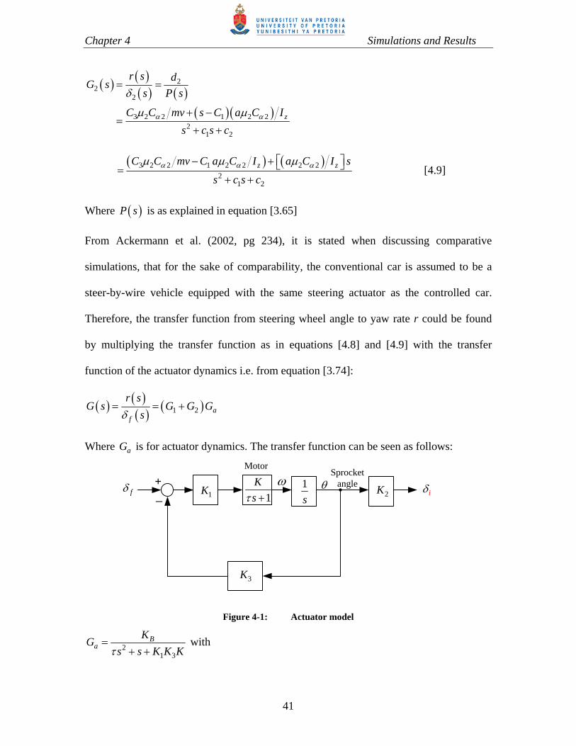
From Ackermann et al. (2002, pg 234), it is stated when discussing comparative
simulations, that for the sake of comparability, the conventional car is assumed to be a
steer-by-wire vehicle equipped with the same steering actuator as the controlled car.
Therefore, the transfer function from steering wheel angle to yaw rate r could be found
by multiplying the transfer function as in equations [4.8] and [4.9] with the transfer
function of the actuator dynamics i.e. from equation [3.74]:
1 2 a
f
r sG s G G G
s
Where aG is for actuator dynamics. The transfer function can be seen as follows:
2K1
s
+_f 1K
1
K
s
Motor
3K
iSprocket
angle
Figure 4-1: Actuator model
21 3
Ba
KG
s s K K K
with

Chapter 4 Simulations and Results
42
1 2BK K K K
The transfer functions for yaw disturbance input from lateral disturbance force dyF and
yaw disturbance moment, DM , will be, (see equation [3.74]):
5
3 1
21 2
Fdy
gp z
r s dG s
F s P s
C mv s C l I
s c s c
[4.10]
3 1
21 2
gp z gp zC mv C l I l I s
s c s c
and
6
12
1 2
MD
z
r s dG s
M s P s
s C I
s c s c
12
1 2
z zs I C I
s c s c
[4.11]
4.3 Results
This section deals with simulated results that were done. The vehicle step responses are
shown where the inputs were lateral force input and yaw disturbance torque.
4.3.1 Validation of the model
In order to check the validity of the model and the code, the system was given similar
inputs and parameters to what Ackermann et al. (2002) did and the results are as shown
in figure 4-2. The simulated results as seen in the graphs compare very well with what is
found in the Ackermann et al. (2002), especially on page 235. The value for torque

Chapter 4 Simulations and Results
43
disturbance input used was 1300Nm while the steering wheel angle step input was 0.13 .
There is a good correlation between these two results and this stems from the fact that the
two models were analysing the same physical system. Simulated results meanings are
well articulated by Ackermann et al. (2002). Fcontr and Fconv have the same meanings as
1 in the nomenclature and figure 3-2, for the controlled vehicle and conventional
vehicle, respectively. Here s is the steering wheel angle.
0 0.2 0.4 0.6 0.8 1 1.2 1.4 1.6 1.8 2-0.5
0
0.5
1
1.5
Time (Sec)
yaw
ra
te (
de
g/s
)
Steering wheel angle response
v = 50m/s, = 1
controlled
conventional
0 0.2 0.4 0.6 0.8 1 1.2 1.4 1.6 1.8 20
0.02
0.04
0.06
0.08
0.1
0.12
0.14
0.16
Time (Sec)
Steering wheel angle response
s,
F [d
eg
]
Fcontr
s
Fconv
0 0.2 0.4 0.6 0.8 1 1.2 1.4 1.6 1.8 2-0.5
0
0.5
1
1.5
2
Time (Sec)
yaw
ra
te (
de
g/s
)
Yaw disturbance torque step response
v = 50m/s, = 1
controlledconventional
0 0.2 0.4 0.6 0.8 1 1.2 1.4 1.6 1.8 2-0.2
-0.15
-0.1
-0.05
0
0.05
Time (Sec)
Yaw disturbance torque step response
s,
F [d
eg
]
Fcontr
Fconv
s
Figure 4-2: Simulation results at 50 1v m s

Chapter 4 Simulations and Results
44
4.3.2 Simulations of a conventional and a decoupled vehicle
All the simulations were based on the assumption that the vehicle was travelling on a dry
ground hence i was taken to be equal to 1. A value of 1500N for step lateral force was
always used while the disturbance yaw moment used was 1950Nm unless otherwise
stated.
For the conventional vehicle with front steering only, figure 4-3, the system shows that it
is oscillatory before coming to the steady state value for both the yaw torque and lateral
side wind disturbance input. As for the decoupled system, the responses show that the
system is able to arrest the continued rotation. The decoupled system with front wheels
being steered, figure 4-4, struggles a little bit as compared to the system that combines
with rear individual wheel steering, figure 4-5. Comparing graphs in figure 4-3 with
graphs in figure 4-4 and figure 4-5, one can notice that the controlled system removes the
effect of the disturbance, and this is evidenced by the zero steady state value, and also the
reduced peak value.
Figure 4-3: Step responses of conventional vehicle with front wheels steering only
0 0.5 1 1.5 2 2.5 30
0.01
0.02
0.03
0.04
0.05
0.06
0.07
0.08
0.09
0.1
Time (sec)
yaw
ra
te (
rad
/s)
Yaw torque disturbance (M D ) input step response
0 0.5 1 1.5 2 2.5 30
0.01
0.02
0.03
0.04
0.05
0.06
0.07
Time (sec)
yaw
ra
te (
rad
/s)
Disturbance lateral force (Fdy
) input step response

Chapter 4 Simulations and Results
45
On comparing graphs 4-4 and 4-5, one will notice that graph 4-4 is oscillatory as
compared to graph 4-5 and their settling time is also slightly different. Of course it can be
noted that there was a price that graph 4-5 paid in that the peak is higher as compared to
graph 4-4. We should keep in mind that both of them are decoupled systems only that one
has both front and rear wheels steered while the other one has only the front wheels
steered.
Figure 4-4: Step responses of robustly decoupled vehicle with front wheel steering only
Figure 4-5: Step responses of robustly decoupled with front wheel steering and individual rear
wheel steering
0 0.5 1 1.5 2 2.5 3 3.5 4 4.5 5-0.01
0
0.01
0.02
0.03
0.04
0.05
0.06
0.07
0.08
Time (sec)
yaw
ra
te (
rad
/s)
Yaw torque disturbance (M D ) input step response
0 0.5 1 1.5 2 2.5 3 3.5 4 4.5 5-0.02
-0.01
0
0.01
0.02
0.03
0.04
Time (sec)
yaw
ra
te (
rad
/s)
Disturbance lateral force (F d y ) input step response
0 1 2 3 4 5 60
0.02
0.04
0.06
0.08
0.1
0.12
0.14
Time (sec)
yaw
ra
te (
rad
/s)
Yaw torque disturbance (M D ) input step response
0 0.5 1 1.5 2 2.5 3 3.5 4 4.5 50
0.01
0.02
0.03
0.04
0.05
0.06
0.07
0.08
Time (sec)
yaw
ra
te (
rad
/s)
Disturbance lateral force (Fd y ) input step response

Chapter 4 Simulations and Results
46
The control laws for the rear wheels that were used in all simulations from section 4.2.1
and section 4.2.2 were 3 3 6def
sK r
s
and 4 4 6def
sK r
s
with 3K and 4K as
desired damping gains and r as the yaw rate and the meanings are described in section
4.2.3. 4 is for the rear right and 3 is for the rear left. The constant used were not the
same and the value used for 3K was 39.6723 10 and the value for 4K was
38.9593 10 . This made it easy to feed signals to left and the right wheels because of its
simplicity. This control law was chosen and used because of its simplicity. Ackerman et
al (1992, 2002) suggested and used something similar to this control law.
The rear wheel steering control angles that are proposed here cannot be accommodated
within the theory derived, but the more general equations that can be used are given in
section 4.3.3.1.
All the cases that have been presented so far under this section assume that all parameters
remain constant and that only the disturbance input to the system changes i.e. either the
input is yaw torque, DM , or lateral force, dyF . Figures 4-6 to 4-9 show the yaw rate
response of the vehicle when subjected to a lateral disturbance force under the current
control laws (unilateral decoupled vehicle response with front wheel steering only), but
with varying friction coefficients, the same friction coefficient being used at each wheel.

Chapter 4 Simulations and Results
47
Figure 4-6: Force input response 1 Figure 4-7: Force input response at .0 9
Figure 4-8: Force input response at .0 7 Figure 4-9: Force input response at .0 4
From the figures 4-6 to 4-9, it can be seen that as is reduced, the maximum yaw rate
increases and similarly, as is increased, maximum yaw rate amplitude also reduces. As
becomes smaller, the system becomes oscillatory and the converse is also true.
4.3.3 New control laws
There was need to come up with new control laws to enhance the concept of individual
wheel steering so that one can control the wheels independently of the other. The whole
0 0.5 1 1.5 2 2.5 3 3.5 4 4.5 50
0.01
0.02
0.03
0.04
0.05
0.06
0.07
0.08
Disturbance lateral force (F d y) input step response
Time (sec)
yaw
ra
te (
rad
/s)
= 1
0 0.5 1 1.5 2 2.5 3 3.5 4 4.5 5-0.01
0
0.01
0.02
0.03
0.04
0.05
0.06
0.07
0.08
0.09
yaw
ra
te (
rad
/s)
Disturbance lateral force (F dy) input step response
Time (sec)
= 0.9
0 0.5 1 1.5 2 2.5 3 3.5 4 4.5 5-0.04
-0.02
0
0.02
0.04
0.06
0.08
0.1 Disturbance lateral force (Fdy ) input step response
Time (sec)
yaw
ra
te (
rad
/s)
= 0.7
0 0.5 1 1.5 2 2.5 3 3.5 4 4.5 5-0.2
-0.15
-0.1
-0.05
0
0.05
0.1
0.15
Disturbance lateral force (Fd y ) input step response
yaw
ra
te (
rad
/s)
Time (sec)
= 0.4

Chapter 4 Simulations and Results
48
idea is to have a method of controlling the wheels that could be steered differently from
each other.
4.3.3.1 Requirements for Control Law Design
According to the understanding of this author, a control law is merely a mathematical
statement that helps in decision making within a control system. It not only "helps", but it
also enforces (or at least tries to enforce) a certain dynamic behaviour. Consider a single
steerable wheel. Let’s say under certain conditions, a driver needs to generate a high
lateral force from the wheel. Ordinarily he will have to increase the steering angle in
order to generate the required steering force. The following were the control laws that
were used in the simulations under this section.
11 12 5 10c
ss
s s
[4.13]
22 12 5 10c
ss
s s
[4.14]
33
23 3 13 6defr s
k k s
[4.15]
44
24 4 14 6defr s
k k s
[4.16]
with
1DP
def
l as r sr s
v
[4.17]
def refr r r [4.18]
The chosen control laws for the rear wheels will ensure that the steering angle increases
when there is an increase in the coefficient of friction and reduces the steering angle
when the coefficient of friction is reduced. This is true provided that 23k and 24k are large

Chapter 4 Simulations and Results
49
relative to 3 13k and 4 14k , respectively. As for the two front steering angle control laws
(equations [4.13] and [4.14]), the choice of the control laws was done to ensure that these
angles return to their zero position in the steady state. These control laws are of the form
of the fading integrator. According to Ackerman et al. (1992, 2002), the use of the fading
integrator is to make sure that the corrective steering returns to zero in the steady state
after the occurrence of the disturbance input. The whole idea is to only have this
occurring for the first second after disturbance input before the driver reacts. It is further
stated that this is desirable and done in order to achieve the same stationary cornering
behaviour that the driver is used to and also to unload the actuator for the corrective
steering. The other notable thing with the usage of fading integrators according to
Ackerman et al. (2002) is that stability problems in the yaw motion are reduced. There
are two types of the fading integrators used by Ackerman et al. (2002) which are second
order and first linear order filters.
In view of the new control laws, equation [3.37] was reworked. Using 1 1s c and
2 2s c equation [3.37] now becomes:
11 1 2 2 3 3 4 4
1 2 2
gp1 1 2 2 3 3 4 43 4 3
4
10
C
1Cy
s c
ds c
r r D
z z z z z z
C C C CFC mvmv mv mv mv
la C a C l C l CC rr MI I I I I I
11 1 2 2 3 3 4 41
1 2 2
gp1 1 2 2 3 3 4 43 4 32
4
10
C
1C y
cs
cd
r r
Dz z z z z z
C C C Cx
C mvmv mv mv mv Fla C a C l C l CC rr x MI I I I I I
Where:

Chapter 4 Simulations and Results
50
1 1 2 21
C Cx
mv
1 1 2 2
2z
a C Cx
I
In all the simulation cases, the value used for step disturbance side (cross) wind force is
1500N and the fading integrator used is 2 5 10
s
s s .
4.3.4 Simulations of different coefficient of friction
Figures 4-10 and 4-11 are vehicle responses when the all the four wheels have the same
coefficient of friction . All the wheels are assumed to be under the same road
conditions.
4-10 Force input response 1
4-11 Force input response at .0 3
Comparing figures 4-10 and 4-11 to figures 4-6 to 4-9, it can be seen that the oscillations
have reduced when considering lower coefficients of friction.
The results given in figure 4-12 show rear wheels steer angle responses. The simulations
that were done in this case are where the left hand side of the vehicle is on the different
0 0.5 1 1.5 2 2.5 3 3.5 4 4.5 50
0.005
0.01
0.015
0.02
0.025
Time (Sec)
Yaw rate response to disturbance force (F d y ) input
yaw
ra
te (
rad
/s)
= 1
0 0.5 1 1.5 2 2.5 3 3.5 4 4.5 5-0.005
0
0.005
0.01
0.015
0.02
0.025
0.03
Yaw rate response to disturbance force (Fdy ) input
Time (sec)
yaw
rat
e (r
ad/s
)
= 0.3

Chapter 4 Simulations and Results
51
road conditions compared the right hand side. For example, the left hand side wheels
could be in mud while the right hand side wheels could be on dry tar mark road. We are
going to monitor what will be happening to the rear wheels ( 3 and 4 ). The coefficient
of friction for the left wheels, corresponding to 1 and 3 , will be the same and will
be varied; at the same time, the coefficient of friction for the right hand side wheels,
corresponding to 2 and 4 , will be the same and it will remain constant at 1.
Figure 4-12: Vehicle disturbances response to different
The results as seen in figure 4-12 show that when two sides are on different road
conditions, the model is able to turn more on the hard side (larger ) and it is also able to
turn less on the side with lower value of coefficient of friction. This shows that it is
possible to control each individual wheel independently.
0.5 1 1.5 2 2.5 3-0.01
-0.005
0
0.005
0.01
0.015
0.02
0.025
0.03
0.035 Rear wheels angles response to disturbance force (F dy
Time (sec)
Rea
r w
heel
ang
les
3 a
nd 4
[ra
d]
v = 50 m/s, 1
, 3 = 0.8; 2
, 4 = 1
3 4
) input
0 0.5 1 1.5 2 2.5 3-0.01
-0.005
0
0.005
0.01
0.015
0.02
0.025
0.03
0.035
Rear wheels angles response to disturbance force (F d y ) input
Time (sec)
Rea
r w
heel
ang
les
3
4 [
rad]
v = 50 m/s,
1 , 3 = 0.5; 2 , 4
= 1
3 4
and

Chapter 5 Implementation of Individual Wheel Steering
52
5 IMPLEMENTATION OF INDIVIDUAL WHEEL STEERING
5.1 Introduction
Theoretical modelling and analysis of an individual wheel steering (IWS) system was
done when all information was gathered both from available literature as well as from the
existing 4WS experimental vehicle that is in the SASOL Lab. This vehicle, figure 5-1,
used to have the normal mechanical front wheel steering while the rear wheels were
controlled through steer by wire. The whole 4WS was reworked in order to achieve
individual wheel angle steering. Electric actuators were installed for both front and rear,
on each wheel, to replace the previous steering system that included electrically actuated
hydraulic power steering on the two rear wheels only.
The rear wheel steering rack with power steering was disabled. Both the front and the
rear tie-rods were replaced by linear actuators. These were designed and built specifically
for this project and the purpose of these linear actuators were to effect the individual
wheel steering control. The normal front wheel steering via the rack and pinion system
was still partly available for the driver to control the front wheel steer angles.

Chapter 5 Implementation of Individual Wheel Steering
53
Figure 5-1: Experimental vehicle
5.2 Motor characterisation
A Bosch wiper motor, including its reduction worm gear box, as used in a BMW 325i
model, as shown in figure 5-2, was used in each of the linear actuators. Furthermore, it is
worth mentioning that one can use either of two methods to control a DC wiper motor: an
armature control or pulse width modulation (PWM). Inside the position feedback control
loop, in the forward path, the DC motor and its control works as a speed control sub-
system, regardless of whether one uses armature control or PWM. The DC motor in
speed control can mathematically be modelled as an armature controlled DC motor and
can be represented as a first order equation as shown in equation [5.1], after

Chapter 5 Implementation of Individual Wheel Steering
54
approximating a aL R , as given by Dorf et al. (2001), equation [2.69], where K and
can be determined experimentally.
1a
s K
V s s
[5.1]
Figure 5-2: Wiper motor sketch
Because of lack of information about this wiper motor, several tests were conducted to
determine its characteristics, primarily the gain K and time constant as shown in
equation [5.1]. Figure 5.3 shows the setup for the determination of the motor
characteristics. A tacho-generator was connected to the shaft of the motor, to generate a
voltage output signal proportional to the motor speed. The output from the tacho-
generator and the input from the motor were measured using a digital oscilloscope. The
data were extracted from the oscilloscope using a computer. Tacho-generator was used
only for the purpose of the characterization exercise. It does not form part of the actual
actuator control system.

Chapter 5 Implementation of Individual Wheel Steering
55
Figure 5-3: Motor tests setup
Figure 5-4 shows the response of the motor to step input. The first experiments done were
to determine motor time constant .This was done in order to find out if the wiper motor
to be used meets the desired requirements.
-0.5 0 0.5 1 1.5 2-8
-6
-4
-2
0
2
4
6Response to step input
Time (s)
Am
plitu
de (
volts
)
Source (step) input
Response
Figure 5-4: Motor response to a step input

Chapter 5 Implementation of Individual Wheel Steering
56
Figures 5-4 shows motor response to a step input and amplitude is in volts. The response
graph has been multiplied by the reciprocal of the DC gain, which is why in the steady
state the two graphs fall on top of one another. From this figure, it can be noted that the
motor attained its steady state in less that 1 sec. This exercise was done to make sure that
motors used fell within the specifications one of which was to be able to attain its steady
state in less than 1 sec. This was open loop input – output relationship. To find the
settling time of the system, locate the time on the plot when the magnitude crosses the
desired percentage of the final value. For instance to find the 10% settling time of this
system, look for where the response reaches 90% of the final value. The time constant,
, of the system is the time at which the response is 1 1/ e times by the final value.
The relationship between the time constant and the pole of a system is: pole = -1 / .
Other handy approximate relations for finding the time constant are:
= 10% Settling Time / 2.3 or
= 5% Settling Time / 3 or
= 2% Settling Time / 4.
From the graphs, the average was found to be equal to 0.1339 sec. This was deemed
acceptable.
The next step was to find the DC gain, K , of the motor. The DC gain is the ratio of the
steady state step response to the magnitude of a step input. The steady state step response
can be determined from the plot of the step response like one shown in figure 5-4. The
value of gain K was found after taking into consideration the calibration value of the
Chapter 5 Implementation of Individual Wheel Steering
57
tacho-generator as well as the gain from gear ratio of the wiper motor gear box. The
average value of DC gain that was found was 9.972 / /rad s v .
5.3 Potentiometer characterisation
For the linear actuator to work properly there was need to create a position control
system, with position feedback of some sort. After considering all the possibilities, it was
decided to measure the angle of rotation of the output shaft of the wipe motor gearbox for
the purposes of position feedback. A multi-turn potentiometer was used for that purpose
as an angular position feedback transducer. Figure 5-5 shows the assembly used in
finding the characteristics of the multi-turn potentiometer that was used as an angle
feedback sensor. The body of the Potentiometer is fixed to the wiper motor chassis to
prevent it from moving. The shaft of the potentiometer was inserted into a cork coupling
that was fixed to the base as shown. When the motor is turning, it rotates the shaft of the
Potentiometer. As the shaft turns, the voltage output can be measured and converted to
the angle that the sprocket has turned.

Chapter 5 Implementation of Individual Wheel Steering
58
Figure 5-5: Potentiometer connection sketch
The unit shown on figure 5-6 shows the actuator as assembled to the vehicle.
Figure 5-6: Actuator unit

Chapter 5 Implementation of Individual Wheel Steering
59
Experiments were done and the relationships below were found by measuring
potentiometer angle, wheel angle and voltage output from the potentiometer. The
calibration of the potentiometer was done by using the dividing head and indexing plate
in the machine shop. The base of the potentiometer was clamped while turning the
indexing plate. The potentiometer had 10 complete turns. Voltage measurements were
taken for every complete turn of the knob of the potentiometer. The results were plotted
for voltages against potentiometer angle.
The next stage was to measure the wheel angle and then measure the potentiometer
voltage. This was done to find the relationship between the potentiometer voltage and the
wheel angle. The first step was to zero all the wheels by aligning them. When the wheels
are aligned, then that is the zero point for the potentiometer. A hard paper was stuck to
the ground and then a straight edge was used to mark a straight line on the paper as the
zero angle. The wheel was then turned using the actuator. The turning was not done
continuously; it was done by starting and stopping the actuator. Every time when the
actuator was stopped, successive lines were drawn using a straight edge on the paper that
was stuck to the ground. Voltage measurements from the potentiometer were taken at
every stop. This was done in both directions of the wheel turning and the same procedure
was repeated on all the four potentiometers and all the four wheels. Angles were read off
from the paper later on. The measured potentiometer voltage values for the wheels angle
were plotted.
A mathematical relationship stemming from linear progression between the turn of the
potentiometer knob for voltage and wheel angle was developed, and this was included in
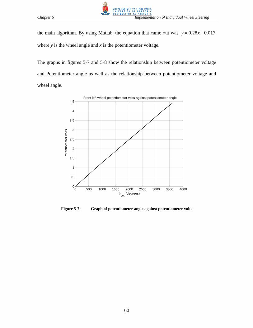
Chapter 5 Implementation of Individual Wheel Steering
60
the main algorithm. By using Matlab, the equation that came out was 0.28 0.017y x
where y is the wheel angle and x is the potentiometer voltage.
The graphs in figures 5-7 and 5-8 show the relationship between potentiometer voltage
and Potentiometer angle as well as the relationship between potentiometer voltage and
wheel angle.
Figure 5-7: Graph of potentiometer angle against potentiometer volts
0 500 1000 1500 2000 2500 3000 3500 40000
0.5
1
1.5
2
2.5
3
3.5
4
4.5
pot (degrees)
Pot
entio
met
er v
olts
Front left wheel potentiometer volts against potentiometer angle

Chapter 5 Implementation of Individual Wheel Steering
61
Figure 5-8: Graph of wheel angle against Potentiometer volts
5.4 DC motor controller
The circuit in figures 5-10 and 5-11 were built to provide an interface between the
computer and the motor. Power is supplied from the car battery through point a (in the
red circle). The signal that controls the speed of the motor enters through point b. Part A
(in green) generates the pulses for the PWM and passes these to the LMD18200 chip,
which drives and controls the speed of the motor. The PWM was used for the DC motor
speed control sub-system. The circuit to generate pulses uses two 555 ICs connected as
shown. A 7805 regulator is included to restrict voltage to and from part A to 5 volts
because the computer voltage signals can only go to the maximum of 5 volts. Pulses from
part A enters part B (in green) through point d. The decision from the computer to change
direction enters the chip at pin number 3 through point c. This tells the chip to turn the
motor either clockwise or anticlockwise.
0 1 2 3 4 5 6 7 8 9 100
0.5
1
1.5
2
2.5
3 Front left wheel steering angle against potentiometer volts
Wheel angle (degrees)
volts

Chapter 5 Implementation of Individual Wheel Steering
62
DC Motor Controller
DC Motor Gain
GainSampler
A/DPID
ControllerSampler
D/A
Referencesignal
Potentiometer
Sprocket angle
Computer
iGain
Lead screw
speed
directionWheel angle
Figure 5-9: Actuator block diagram.
Figure 5-9 shows a single actuator block diagram. All that is inside the dashed line was
implemented in the computer and a single computer was used for all four actuators and
also to run the control algorithm, which determined the input/reference signal to all four
actuators. The gain after the integrator is the gear ratio of the worm gear. Downstream of
the point where the sprocket feedback angle is picked, there is a gain block containing the
pitch of the lead screw that translates the sprocket rotation angle into a rectilinear
displacement, (the chain drive had a gain of 1).

Chapter 5 Implementation of Individual Wheel Steering
63
31TIP C
Transistor
220k
1k
1k
470k220 F
1k
1 414N
DIODE
0V
12V
8
51
74
1 5
8
2
3
47
2,63 6
1k
0.1 F0.1 F 0.01 F
M12 V DC Motor
ReverseForward
31
1110
5
2220 F
1 F6
7LMD18200
From computerFor direction
4
From computerfor proportional
Voltage
7805
10k
1 F
1 F
a
b
c
e
d
555555
Regulator
PWM
Figure 5-10: DC Motor Controller circuit diagram
Figure 5-11: DC motor Controller circuit box

Chapter 5 Implementation of Individual Wheel Steering
64
A cooling fan was used to cool down the LMD18200 chip, which otherwise overheats
and then shuts itself down
Figure 5-12: Illustrating the principle of Pulse Width Modulation, National Semiconductors
(2005)
Figure 5-12 shows the concept of PWM. If the motor is to turn at full speed, the system
has to supply 100% duty cycle pulses. In order to reduce the speed of the motor, there
should be a supply of pulses as shown in figure 5-12 depending on the desired speed.
LMD
1820
0
Figure 5-13: LMD18200 chip, National Semiconductors (2005)
Figure 5-13 shows an LMD18200 chip which works as an H-Bridge as illustrated in
figure 5-14.
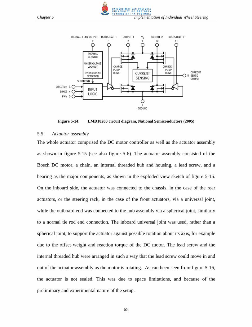
Chapter 5 Implementation of Individual Wheel Steering
65
Figure 5-14: LMD18200 circuit diagram, National Semiconductors (2005)
5.5 Actuator assembly
The whole actuator comprised the DC motor controller as well as the actuator assembly
as shown in figure 5.15 (see also figure 5-6). The actuator assembly consisted of the
Bosch DC motor, a chain, an internal threaded hub and housing, a lead screw, and a
bearing as the major components, as shown in the exploded view sketch of figure 5-16.
On the inboard side, the actuator was connected to the chassis, in the case of the rear
actuators, or the steering rack, in the case of the front actuators, via a universal joint,
while the outboard end was connected to the hub assembly via a spherical joint, similarly
to a normal tie rod end connection. The inboard universal joint was used, rather than a
spherical joint, to support the actuator against possible rotation about its axis, for example
due to the offset weight and reaction torque of the DC motor. The lead screw and the
internal threaded hub were arranged in such a way that the lead screw could move in and
out of the actuator assembly as the motor is rotating. As can been seen from figure 5-16,
the actuator is not sealed. This was due to space limitations, and because of the
preliminary and experimental nature of the setup.

Chapter 5 Implementation of Individual Wheel Steering
66
Figure 5-15: Actuator – hub assembly connection
Figure 5-15 shows one actuator, connected to the right rear wheel, replacing the right rear
tie rod of the original four wheel steering system.
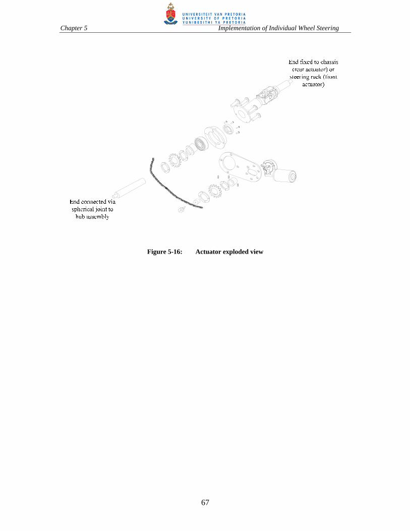
Chapter 5 Implementation of Individual Wheel Steering
67
Figure 5-16: Actuator exploded view

Chapter 6 Experiments and Results
68
6 EXPERIMENTAL SETUP
This chapter describes the experimental setup, experimental tests that were carried out
and the results that were obtained. Experimental tests were done for the individual wheel
steering system. These tests were before expanding the mathematical model and
therefore the tests did not implement the new control laws that are described in equations
[4.13] to [4.18]. In other words, control laws equations [4.13] to [4.18] were never tested
experimentally. More also, the experimental setup, as depicted in figure 6-1, used control
law equation [3.50] for the front wheels and the rear wheel control laws mentioned on
page 47, below figure 4-9.
r
yDPa
2c
3
4
DM dyF
s refr
1c
Figure 6-1: A sketch of experimental setup

Chapter 6 Experiments and Results
69
Figure 6-1 shows the experimental setup diagrammatically. Each wheel was controlled
individually via the computer. The feedback signal from lateral acceleration shown was
not used for any purpose although it is one of the outputs as shown in equation [3.70]. A
yaw rate sensor was connected on the vehicle to measure the yaw rate for feedback
purposes but also to have a measurable result.
Figure 6-2: Computer
Figure 6-2 shows a computer that was used for experiments. The output of this computer
can be both analogue and digital, because it was equipped with an analogue to digital
card. In this experiment, one analogue and one digital output was used for each steering
actuator. The analogue output was used for control voltage while the digital output was
used to switch direction of the dc motor in the actuator. The output voltage from the
computer was used to change the speed of the motor. If the digital output was 0 the motor
turned in one direction and if the output was 1 the motor turned in the opposite direction.
Computer

Chapter 6 Experiments and Results
70
6.1 Experimental Results
There were two sets of experiments that were conducted to validate the proposed theories
as will be discussed in section 6.1.1 and section 6.1.2. The driver kept the steering wheel
straight in most of the tests that were done. The exceptions were on a number of tests
where the driver had to induce sinusoidal input from the steering wheel. This was to
ensure that there is separation of the driver task and that of control system. The driver’s
job had to do with path tracking while the control system had to control the yaw rate.
6.1.1 No input from the steering wheel
It was decided to employ uneven braking between the left and right wheels to induce a
disturbance moment on the vehicle during road tests. For this purpose the brake calliper
of the left front wheel was taken off the disk, thus disabling braking on that wheel. The
driver then had to brake hard to induce a disturbing moment. The advantage of using this
method to generate a yaw moment is that it is cheap. On the other hand, it is unlikely that
this scenario will be encountered in a real life situation. It was done purely for
experimental purposes. Instead, it would have been better to use wind generators to create
side wind disturbance, but such generators were not available. The results provided in
figures 6-3 to 6-9 are from the test run that was seen to be successful. The only known
parameter is the speed since the successful test was done at a speed of 50 km/h at the time
of braking. It was difficult to measure other parameters like the generated yaw torque
from braking. The other tests were partially successful while other tests were not very
successful as will be highlighted later.

Chapter 6 Experiments and Results
71
Figure 6-3: Controlled vehicle yaw rate response.
Figure 6-3 shows the comparison between simulated and experimental results. The brakes
were applied when the vehicle was travelling at a speed of 50 km/h. Because of lack of
other information, and lack of measuring methods, some of the parameters were assumed
for simulation purposes. For example, to know how much brake force and the size of
yaw moment created during the period that the brakes were applied, were difficult.
Figures 6-4 to 6-7 show the comparison between the experimental and the simulated
results of each wheel.
0 0.5 1 1.5 2 2.5 3 3.5 4 4.5 5 -5
-4
-3
-2
-1
0
1
2
3
4
5
Yaw
Rat
e (o
/sec
)
Time
Yaw Rate Response With Control
Experimental Results
Simulation Results

Chapter 6 Experiments and Results
72
Figure 6-4: Front right additional steering angle response
Figure 6-5: Front left additional steering angle response
1 1.5 2 2.5 3 3.5 4 4.5 5 -1
-0.8
-0.6
-0.4
-0.2
0
0.2
0.4
Time
Ste
erin
g A
ngle
s (
Deg
rees
)
Steering Angles Results
c1 ---> Experiment
c1 ---> Simulation
0 0.5 1 1.5 2 2.5 3 3.5 4 4.5 5 -1.6
-1.4
-1.2
-1
-0.8
-0.6
-0.4
-0.2
0
0.2
0.4 Steering angles results
time
Ste
erin
g an
gle
s (D
egre
es)
--> Experiment
--> Simulation

Chapter 6 Experiments and Results
73
Figure 6-6: Rear right steering angle response
Figure 6-7: Rear left steering angle response
0 0.5 1 1.5 2 2.5 3 3.5 4 4.5 5 -1.6
-1.4
-1.2
-1
-0.8
-0.6
-0.4
-0.2
0
0.2
0.4
Time
Ste
erin
g A
ngle
s (
Deg
rees
)
Steering Angles Results
4 ---> Experiment
4 ---> Simulation
0 0.5 1 1.5 2 2.5 3 3.5 4 4.5 5 -1.4
-1.2
-1
-0.8
-0.6
-0.4
-0.2
0
0.2
0.4
Ste
erin
g A
ngle
s (
Deg
rees
)
Time
Steering Angles Results
3 ---> Experiment
3 ---> Simulation

Chapter 6 Experiments and Results
74
6.1.2 Sinusoidal input from the steering wheel
Figures 6-8 and 6-9 show the yaw rate response of the test vehicle to sinusoidal input that
was done through the steering wheel with the control system either inoperative (figure 6-
8) or operative (figure 6.9) and the vehicle travelling at 50 km/h. The reason why a
sinusoidal input test was done was because it was thought that the controlled system
could be fooled to think that the yaw that resulted from the driver giving a sinusoidal
steering input was actually some disturbance that it should reject. Hence we expected
that a successful test would be indicated by a reduced amplitude in the sinusoidal yaw
rate variation, in the case of the controlled car. That the yaw rate would reduce to zero
after the test is not an indication of success, because any stable motorcar will have a zero
yaw rate in the steady state after a sinusoidal steering input was removed. From figure 6-
9, it can be seen that the controlled car has a smaller variation in yaw rate than the
uncontrolled car, figure 6-8. The test driver tried to use the same magnitude of sinusoidal
excitation in the two cases, even though this is a subjective measure.

Chapter 6 Experiments and Results
75
Figure 6-8: Uncontrolled vehicle test result at 50 km/h
Figure 6-9: Controlled vehicle test result at 50 km/h
0 0.5 1 1.5 2 2.5 3 3.5 4 4.5 5-8
-6
-4
-2
0
2
4
6
8
10
12Yaw rate sinusoidal input response - Uncontrolled
Time (sec)
Yaw
rat
e (D
egre
es/s
)
0 0.5 1 1.5 2 2.5 3 3.5 4 4.5 5-1.5
-1
-0.5
0
0.5
1
1.5
2Yaw rate sinusoidal input response - Controlled
Time (sec)
Yaw
rat
e (D
egre
es/s
)

Chapter 6 Experiments and Results
76
There were other tests that were done at lower speeds, the results of which showed that
the rear wheels did not respond satisfactorily, as shown in the figure 6-10. It was
observed that at lower speeds, the rear wheels failed to respond presumably because of
weight. The engine of the vehicle is mounted at the rear and as a result it was hard for the
wiper motors at the back to steer the rear wheels at the lower speeds. It can be noted that
the response from the front wheels is very small. This may also mean that the command
signal to the two rear actuators was within the dead band of the rear actuators. The
higher vertical wheel loading on the rear wheels due to the engine weight would have
caused a larger dead band in the case of the rear wheels, compared to the front.
Figure 6-10: Steering angles response at low speed (20 km/h)
Figure 6-10 shows a test result that was conducted at an approximate sinusoidal
disturbance input through the steering wheel while the vehicle was travelling at a speed
of 20 km/h. The 3 and 4 curves are not responding the same perhaps because the
0 0.5 1 1.5 2 2.5 3 3.5 4 4.5 5-0.2
-0.15
-0.1
-0.05
0
0.05
0.1
0.15
Time
Ste
erin
g A
ngle
s (
Deg
rees
)
Steering Angles - Experimental Results
c 1 c 2 3
4

Chapter 6 Experiments and Results
77
vertical wheel loading are not the same (see the measured loads shown on the very last
page of this report) bearing in mind the low speed at which the vehicle was travelling.
Figure 6-11: Steering angles responses to braking at 40 km/h
Figure 6-11 shows the steering angles recorded while disturbing the vehicle with braking
from 40 km/h. It shows that all the wheels managed to return to zero steer position
though quite slowly.
0 0.5 1 1.5 2 2.5 3 3.5 4 4.5 5-0.8
-0.6
-0.4
-0.2
0
0.2
0.4
0.6 Steering Angles - Experimental Results
Time
Ste
erin
g A
ngle
s (
Deg
rees
)
c1
c2
3
4

Chapter 7 Conclusions
78
7 CONCLUSIONS AND FUTURE WORK
The research work has measured and presented some results, of which the conditions to
make a full correlation study between measurement and numerical prediction is not
known, but at least the work can show simulation results that quantitatively look quite
similar, and the conditions that pertain to this simulation is quite realistic, i.e., it would
have been possible to have made an experiment with matching conditions.
It can be noted from the theories presented that under dissimilar conditions at the wheels,
in order to give a true picture of the actual vehicle, every wheel has to be treated
individually. When one is driving or steering, wheels are in contact with the ground
independently. Even the load (weight) distribution of the vehicle is not the same on all
the wheels as evidenced from the measurement results of the experimental vehicle. When
wheels are not treated as a single entity, like in the bicycle model, some information is
bound to be lost. In this dissertation a steering control analysis has been presented,
similar to that of Ackermann, but with each wheel treated on its own. In addition to this,
the modelling of a side wind acting at the centre of pressure was included in the analysis.
The model that has been investigated is clearly an improvement of the bicycle model that
has been used extensively by researchers in the understanding the concepts of 4WS. The
results from simulations indicate that now it is possible to control each wheel
independently. We have seen an improvement in the vehicle response by individually
controlling the wheels as compared to the conventional steering. With control laws based
on the bicycle model, the vehicle tends to oscillate, especially at lower coefficients of
friction. The independent steering control laws in this work were shown to result in larger
stability margins (fewer oscillations) even at lower coefficients of friction. The cases that

Chapter 7 Conclusions
79
were investigated in this work are generic in that they were not condition specific,
because it is now possible to investigate different road conditions at the left and right
hand side wheels.
From the results presented, the wheels are able to return to their zero steering angle
position after the effect of a disturbance was rejected. It was important to make sure that
no steering angle remains after action of the control system. This highlights the ability of
this experimental vehicle to reject disturbances.
There were some problems with the experimental results obtained. The results were
deficient in terms of repeatability because of the configurations and characteristics of the
wiper motors used. Firstly, there were slight differences between clockwise and anti-
clockwise characteristic responses of the wiper motors used. Secondly, at low speeds, the
motors could not push hard enough to generate the required angles. Another problem was
that the yaw rate sensor used had significant inherent noise. Otherwise, given all
conditions to be ideal, with this method, there is a possibility to achieve disturbance
rejection.
Since one of the objectives was to be able to steer the wheels individually, and this was
met, one can take advantage of that to further the research. On the experimental side, it
will now be easier to let the wheels be on different road conditions and monitor the
performance. More also, one can do further tests like subjecting the vehicle to different
road manoeuvres e.g. double lane changes, parallel parking, and side gust response
measurements, if side wind generating tunnels were to be made available. Future work
can benefit from employing more suitable actuators, because the type of motors that were

Chapter 7 Conclusions
80
used were essentially underpowered and the performance and response of the motors in
clockwise and anticlockwise directions were observed to be different. One can also think
of improving the system modelling by using the equations in their nonlinear form,
especially with respect to simulation, and see if there will be any improvements (or
perhaps deteriorations) compared to the linearized equations analysis. The extension of
this work into nonlinear regime should also look at more sophisticated tyre models. The
vehicle dynamics modelling also needs to be expanded to include roll dynamics, with the
associated load transfer. This will be important if manoeuvres like double lane changes
were to be simulated. More also, the control laws [4.13] to [4.18] that were investigated
in simulations, assumed that the friction coefficient at each wheel is known. It is,
however, quite difficult (if not impossible) to measure, in real time, the friction
coefficient in order to implement these control laws. This is one of the major
disadvantages of the proposed control laws. Therefore, one can also do a research and
look into practical ways on how to estimate the friction coefficient, if the uses of these
control laws are to be further employed.

References
81
REFERENCES
Abe, M. (1999). Vehicle dynamics and control for improving handling and active safety:
from four wheel steering to direct yaw moment control. Proc Instn Mech Engrs. Vol. 213
Park K, pp. 87-101.
Abe, M., and Mokhiamar, O. (2002). Active wheel steering and yaw moment control
combination to maximize stability as well as vehicle responsiveness during quick lane
change for active vehicle handling safety. Proc Instn Mech Engrs, Vol. 216 part D: J
Automobile Engineering, pp. 115-124.
Ackermann, J. and Bunte, T. (1997). Yaw disturbance attenuation by robust decoupling
of car steering. Control Engineering Practice, (pp.1131-1136).
Ackermann, J., (1992) Robust yaw damping of cars with front and rear wheel steering,
Proceedings of the 31st Conference Declalon and Control, Tucson, Arizona, pp. 2586-
2590.
Ackermann, J., Bunte, T., and Odenthal, D. (1999). Advantages of active steering for
vehicle dynamics control. Proc. 32nd International Symposium on Automotive
Technology and Automation, pages 263-270, Vienna.
Ackermann, J. and Bunte, T. (1995). Automatic car steering control bridges of the driver
reaction time. Institute for robotics and system dynamics, Germany.
Ackermann, J. and Bunte, T. (1996). Driving safety by robust steering control. Proc. Int.
Symposium on Advanced Vehicle Control, (Aachen, Germany).

References
82
Ackermann, J., in co-operation with Blue, P., Bunte, T., Guvenc, L. Kaesbauer, D.,
Kordt, M., Muhler, M. and Odenthal D. (2002). Robust control: The variable space
approach. Second Edition, Springer-Verlag.
Ackermann, J., Walter, W., and Bunte, T. (2004). Automatic car steering using robust
unilateral decoupling. International Conference on Advances in Vehicle Control and
Safety, Genoa, Italy.
Dorf, R.C. and Bishop, R.H. (2001). Modern Control Systems, International Edition.
Ninth Edition. Prentice – Hall, Inc.
Friedland, B. (1986). Control system design – An introduction to state space methods.
McGraw-Hill Publishing Company.
Ghelardoni, M. (2004). Feasibility study of yaw control by active 4 - wheel drive. Thesis,
Technische Universiteit Delft.
Genta, G. (1997). Motor vehicle dynamics – Modelling and simulation. World Scientific
Publishing Co. Pty. Ltd.
Gillespie, T.D. (1992) Fundamentals of vehicle dynamics. Warrendale, P.A., Society of
Automotive Engineers.
Hanke, O. Bertram, T. and Hiller, M. (2001). Analysis and control of vehicle dynamics
under crosswind conditions. IEEE/ASME International Conference on Advanced
Intelligence Mechatronics Proceedings, Italy, pp 331 – 336.

References
83
Hucho, W.H. (1987). Aerodynamics of road vehicles. Butterworth. Printed in Great
Britain at University Press, Cambridge.
Kitajima, K., and Peng, H. (2000). H control for integrated side-slip, roll and yaw
controls for ground vehicles. Proceedings of Avec 2000 5th International Symposium on
Advanced Vehicle Control, August 22-24, Ann Arbor, Michigan.
Klein, S. (1996). Active control of a four wheel steered vehicle. MEng. Dissertation,
University of Pretoria.
Lakkad, S. (2004). Modelling and simulation of steering system for autonomous vehicles.
Thesis, Florida State University, Collage of Engineering.
Lv H.M, Chenl, N. and LI P.I. (2004). Multi-objective H optimal control for four wheel
steering vehicle based on yaw rate tracking. Proc. Institution of Mechanical Engineers,
Vol. 218 Part D, Automobile Engineering, pp. 1117-1123.
Lynch, D.P. (2000). Velocity scheduled driver assisted control of a four wheel steer
vehicle. Thesis, University of Illinois at Urbana-Campaign.
National Semiconductor Corporation, (2005). LMD18200 3A, 55V H-Bridge. SAE J670e (1976). Vehicle dynamics terminology. Wong, J.Y. (1993). Theory of ground vehicles. Second Edition, John Willy & Sons Inc.

References
84
Wu, D., Zhang, Q. and Reid, J.F. (2001). Adaptive steering controller using Kalman
estimator for wheel-type agricultural tractors. Robotica Vol. 19, pp. 527-533.
Cambridge University Press.
You, S.S., and Joeng, S.K. (1998). Vehicle dynamics and control synthesis for four wheel
steering passenger cars. Proc Institution of Mechanical Engineers, Vol. 212 Part D, pp.
449-461.
Zhengqi, L., Yufeng, L. and Seemann, W. (2003). The performance of a vehicle with four
wheel steering control in cross wind. International Journal Of Vehicle Autonomous
Systems (IJVAS), Vol. 1, No. 2. pp. 256-269.

Appendix
85
APPENDIX
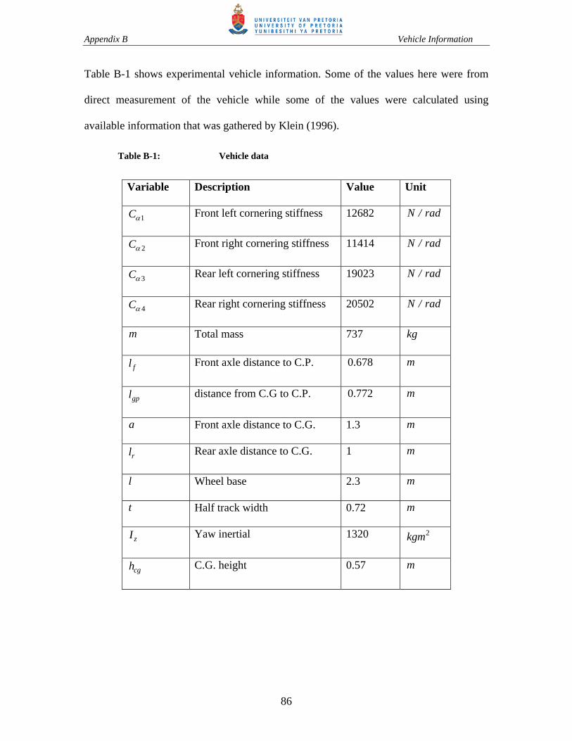
Appendix B Vehicle Information
86
Table B-1 shows experimental vehicle information. Some of the values here were from
direct measurement of the vehicle while some of the values were calculated using
available information that was gathered by Klein (1996).
Table B-1: Vehicle data
Variable Description Value Unit
1C Front left cornering stiffness 12682 N / rad
2C Front right cornering stiffness 11414 N / rad
3C Rear left cornering stiffness 19023 N / rad
4C Rear right cornering stiffness 20502 N / rad
m Total mass 737 kg
fl Front axle distance to C.P. 0.678 m
gpl distance from C.G to C.P. 0.772 m
a Front axle distance to C.G. 1.3 m
rl Rear axle distance to C.G. 1 m
l Wheel base 2.3 m
t Half track width 0.72 m
zI Yaw inertial 1320 2kgm
cgh C.G. height 0.57 m

Appendix B Vehicle Information
87
The values below are the static vertical wheel forces of the experimental vehicle that
were found after measuring with wheel scales:
1 146.03zF kgf
2 139.68zF kgf
3 210.431zF kgf
4 244.44zF kgf