Model-checking Quantitative Alternating-time

Temporal Logic on One-counter Game Models

Steen Vester

Technical University of Denmark, Kgs. Lyngby, Denmark

Abstract

We consider quantitative extensions of the alternating-time tempo-ral logics ATL/ATL∗ called quantitative alternating-time temporal logics(QATL/QATL∗) in which the value of a counter can be compared toconstants using equality, inequality and modulo constraints. We interpretthese logics in one-counter game models which are infinite duration gamesplayed on finite control graphs where each transition can increase or de-crease the value of an unbounded counter. That is, the state-space of thesegames are, generally, infinite. We consider the model-checking problemof the logics QATL and QATL∗ on one-counter game models with VASSsemantics for which we develop algorithms and provide matching lowerbounds. Our algorithms are based on reductions of the model-checkingproblems to model-checking games. This approach makes it quite sim-ple for us to deal with extensions of the logical languages as well as theinfinite state spaces. The framework generalizes on one hand qualita-tive problems such as ATL/ATL∗ model-checking of finite-state systems,model-checking of the branching-time temporal logics CTL and CTL∗ onone-counter processes and the realizability problem of LTL specifications.On the other hand the model-checking problem for QATL/QATL∗ gen-eralizes quantitative problems such as the fixed-initial credit problem forenergy games (in the case of QATL) and energy parity games (in the caseof QATL∗). Our results are positive as we show that the generalizationsare not too costly with respect to complexity. As a byproduct we obtainnew results on the complexity of model-checking CTL∗ in one-counterprocesses and show that deciding the winner in one-counter games withLTL objectives is 2ExpSpace-complete.

1 Introduction

The alternating-time temporal logics ATL and ATL∗ [1] are used to specify tem-poral properties of systems in which several entities interact. They generalize thewidely applied linear-time temporal logic LTL [22] and computation tree logicsCTL [9] and CTL∗ [11] to a multi-agent setting. Indeed, it is possible to specifyand reason about what different coalitions of agents can make sure to achieve.The model-checking problem for alternating-time temporal logics subsumes therealizability problem for LTL [23, 24] which is the problem of deciding whetherthere exists a program satisfying a given LTL specification no matter how the

1

environment behaves. This is closely related to the synthesis problem which con-sists of generating a program meeting such a specification. Properties in theselogics are inherently qualitative and the model-checking problem for alternating-time temporal logics has primarily been treated in finite-state systems. How-ever, in [7] extensions of ATL and ATL∗ to the quantitative alternating-timetemporal logics QATL and QATL∗ have been introduced. The purpose is tomake the languages capable of expressing quantitative properties of multi-agentscenarios as well as deal with infinite-state systems. These are represented us-ing unbounded counters in addition to a finite set of control states. Naturally,this leads to undecidability in many cases since already deciding the winner ina reachability game on a two-dimensional vector addition system with states(VASS) can already simulate the halting problem of a two-counter machine [6].In order to regain decidability we focus on the subproblem of a single unboundedcounter. This is a significant restriction from the multi-dimensional case, butit still lets us express many interesting properties of infinite-state multi-agentsystems. For instance, the model-checking problem includes problems such asenergy games [3] and energy parity games [8] in which a system respectivelyneeds to keep an energy level positive and needs to keep an energy level positivewhile satisfying a parity condition. These are expressible in QATL and QATL∗

as 〈〈Sys〉〉G(r > 0) and 〈〈Sys〉〉(G(r > 0)∧ϕparity) respectively where r is used todenote the current value of the counter. It can be compared to constants usingrelations in {<,≤,=,≥, >}. ϕparity is a parity condition expressed as an LTLformula. It is quite natural to model systems with a resource (e.g. battery level,time, money) using a counter where production and consumption correspond toincreasing and decreasing the counter respectively.

Let us give another example of a QATL specification. Consider the game inFigure 1 modelling the interaction between the controller of a vending machineand an environment. The environment controls the rectangular states and thecontroller controls the circular state. Initially, the environment can insert a coinor request coffee. Upon either input the controller can decrease or increase thebalance, dispense coffee or release control to the environment again.

• Insert coin

Request coffee

Decrease

Increase

Dispense

Release-1

+1

Figure 1: Model of interaction between a vending machine controller and anenvironment.

Some examples of specifications in QATL∗ using this model are

• 〈〈{ctrl}〉〉G(Request ∧ (r < 3) → XXRelease): The controller can makesure that control is released immediately whenever coffee is requested andthe balance is less than 3.

2

• 〈〈{ctrl}〉〉G(Request ∧ (r ≥ 3) → FDispense): The controller can makesure that whenever coffee is requested and the balance is at least 3 theneventually a cup of coffee is dispensed.

1.1 Contribution

The contribution of this paper is to present algorithms and complexity resultsfor model-checking QATL and QATL∗ in one-counter game models with one-dimensional VASS semantics, meaning that transitions that would make thecounter go below zero are disabled. The complexity is investigated both interms of whether only edge weights in {−1, 0,+1} can be used or if we allowany integer weights encoded in binary. We also distinguish between data com-plexity and combined complexity. In data complexity, the formula is assumedto be fixed whereas in combined complexity both the formula and the game areparameters. We characterize the complexity of the model-checking problemsthat arise from these distinctions for both QATL and QATL∗. In most of thecases the complexity results are quite satisfying compared with other resultsfrom the litterature. As a byproduct we also obtain precise data complexity formodel-checking CTL∗ in one-counter processes (OCPs) and succinct one-counterprocesses (SOCPs). In addition, we show that the complexity of deciding thewinner in a one-counter game with LTL objectives is 2ExpSpace-complete.The complexity results encountered range from PSpace to 2ExpSpace, anoverview of the results can be seen in Section 6. The algorithms are based onmodel-checking games which makes it simple for us to handle the extensions ofthe logics considered as well as dealing with infinite state spaces and nesting ofstrategic operators.

1.2 Related work

The realizability problem for LTL was shown to be 2ExpTime-complete in[23, 24]. As this problem is subsumed in QATL∗ model-checking this gives usan immediate 2ExpTime lower bound for the combined complexity of QATL∗

model-checking. The results for realizability of LTL specifications are gener-alized to quantitative objectives in [2] where LTL objectives combined witha mean-payoff objective or an energy objective are considered. However, thesemantics in their setting differs from ours in the way the counter value is han-dled when it gets close to 0. In our setting VASS semantics is used which isnot the case in their setting. Our setting is equivalent to one-dimensional VASSgames considered in e.g. [6]. Deciding the winner in games played on pushdownprocesses with parity objectives and LTL objectives were shown to be ExpTime-complete and 3ExpTime-complete in [27] and [19] respectively. Their settingis the same as ours except that in our setting a singleton stack alphabet is usedto obtain one-counter games. In [25] it was shown that deciding the winner inone-counter parity games is in PSpace. It follows from [6] that this problem isPSpace-complete since selective zero-reachability in 1-dimensional VASS gamesis PSpace-hard. The approaches of module checking [18] and in particularpushdown module checking [5] are related to our setting and have given inspi-ration for our 2ExpSpace-hardness proof of model-checking QATL∗. To com-pare, pushdown module checking of CTL and CTL∗ are 2ExpTime-completeand 3ExpTime-complete respectively. Our problems generalize several model-

3

checking problems of branching-time logics in one-counter processes and are re-lated to model-checking in pushdown processes as well. Model-checking of CTL∗

on pushdown processes has been shown decidable [13], to be in 2ExpTime [12]and to be 2ExpTime-hard [4]. On the other hand, model-checking CTL insuccinct one-counter processes is ExpSpace-complete [14]. Other related linesof research includes model-checking of Presburger LTL [10] where counter con-straints similar to (and more general than) ours are considered in the linear-timeparadigm.

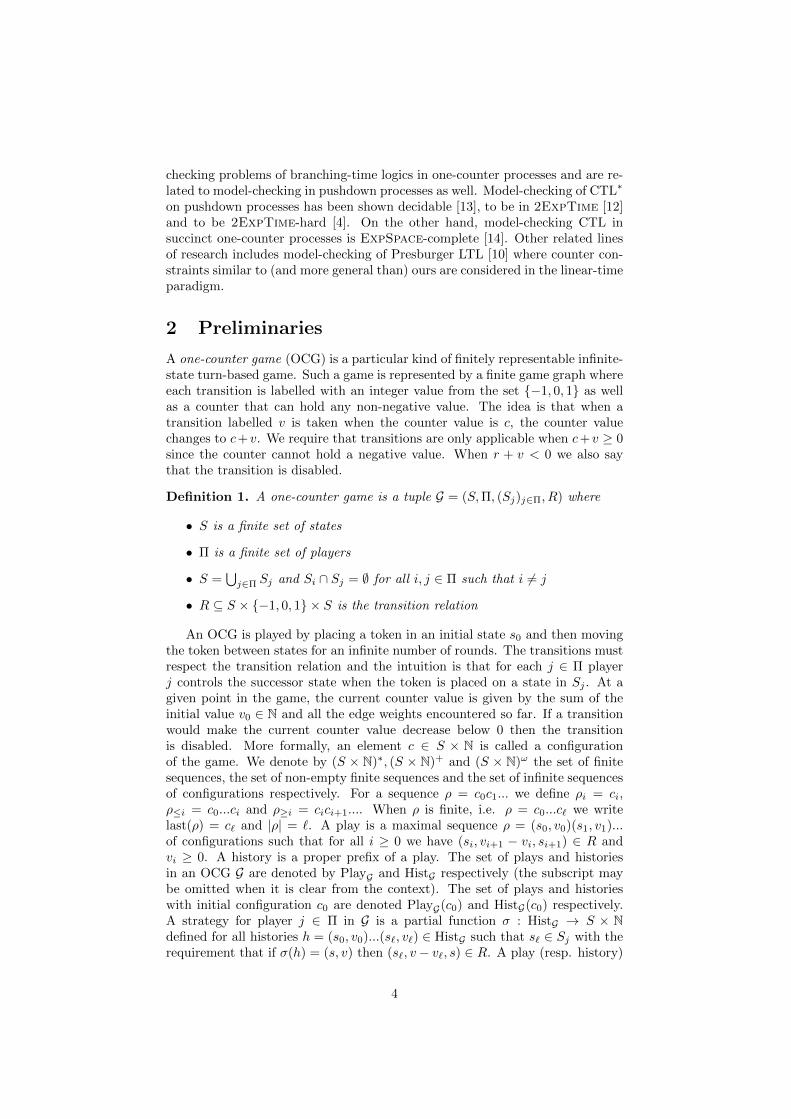
2 Preliminaries

A one-counter game (OCG) is a particular kind of finitely representable infinite-state turn-based game. Such a game is represented by a finite game graph whereeach transition is labelled with an integer value from the set {−1, 0, 1} as wellas a counter that can hold any non-negative value. The idea is that when atransition labelled v is taken when the counter value is c, the counter valuechanges to c+v. We require that transitions are only applicable when c+v ≥ 0since the counter cannot hold a negative value. When r + v < 0 we also saythat the transition is disabled.

Definition 1. A one-counter game is a tuple G = (S,Π, (Sj)j∈Π, R) where

• S is a finite set of states

• Π is a finite set of players

• S =⋃

j∈Π Sj and Si ∩ Sj = ∅ for all i, j ∈ Π such that i 6= j

• R ⊆ S × {−1, 0, 1} × S is the transition relation

An OCG is played by placing a token in an initial state s0 and then movingthe token between states for an infinite number of rounds. The transitions mustrespect the transition relation and the intuition is that for each j ∈ Π playerj controls the successor state when the token is placed on a state in Sj . At agiven point in the game, the current counter value is given by the sum of theinitial value v0 ∈ N and all the edge weights encountered so far. If a transitionwould make the current counter value decrease below 0 then the transitionis disabled. More formally, an element c ∈ S × N is called a configurationof the game. We denote by (S × N)∗, (S × N)+ and (S × N)ω the set of finitesequences, the set of non-empty finite sequences and the set of infinite sequencesof configurations respectively. For a sequence ρ = c0c1... we define ρi = ci,ρ≤i = c0...ci and ρ≥i = cici+1.... When ρ is finite, i.e. ρ = c0...c` we writelast(ρ) = c` and |ρ| = `. A play is a maximal sequence ρ = (s0, v0)(s1, v1)...of configurations such that for all i ≥ 0 we have (si, vi+1 − vi, si+1) ∈ R andvi ≥ 0. A history is a proper prefix of a play. The set of plays and historiesin an OCG G are denoted by PlayG and HistG respectively (the subscript maybe omitted when it is clear from the context). The set of plays and historieswith initial configuration c0 are denoted PlayG(c0) and HistG(c0) respectively.A strategy for player j ∈ Π in G is a partial function σ : HistG → S × Ndefined for all histories h = (s0, v0)...(s`, v`) ∈ HistG such that s` ∈ Sj with therequirement that if σ(h) = (s, v) then (s`, v− v`, s) ∈ R. A play (resp. history)

4

ρ = c0c1... (resp. ρ = c0...c`) is compatible with a strategy σj for player j ∈ Πif σj(ρ≤i) = ρi+1 for all i ≥ 0 (resp. 0 ≤ i < `) such that ρi ∈ Sj × N. We

denote by StratjG the set of strategies of player j in G. For a coalition A ⊆ Πof players a collective strategy σ = (σj)j∈A is a tuple of strategies, one for each

player in A. We denote by StratAG the set of collective strategies of coalition A.For an initial configuration c0 and collective strategy σ = (σj)j∈A of coalitionA we denote by Play(c0, σ) the set of plays with initial configuration c0 that arecompatible with σj for every j ∈ A.

We extend one-counter games such that arbitrary integer weights are allowedand such that transitions are still disabled if they would make the counter gobelow zero. Such games are called succinct one-counter games (SOCGs). Wesuppose that weights are given in binary. The special cases of OCGs and SOCGswhere Π is a singleton are called one-counter processes (OCPs) and succinctone-counter processes (SOCPs) respectively. A game model M = (G,AP, L)consists of a (one-counter or succinct one-counter) game G, a finite set AP ofatomic proposition symbols and a labelling L : S 7→ 2AP of the states S of thegame G with atomic propositions. We abbreviate one-counter game models andsuccinct one-counter game models by OCGM and SOCGM respectively.

By a one-counter parity game we mean the particular kind of one-countergame model where there are two players I and II and the set of propositions is afinite subset of the natural numbers, called colors. Further, every control stateis labelled with exactly one color. In such a game, player I wins if the least coloroccuring infinitely often is even. Otherwise player II wins. We assume that thecounter value is 0 initially and that there is a designated initial state in a one-counter parity game. It was shown in [25] that the winner can be determined ina one-counter parity game in polynomial space by a reduction to the emptinessproblem for alternating two-way parity automata [26].

Proposition 2. Determining the winner in one-counter parity games is inPSpace.

3 Quantitative Alternating-time temporal logic

We consider fragments of the quantitative alternating-time temporal logics QATLand QATL∗ introduced in [7] interpreted over one-counter game models. Thelogics extend the standard ATL and ATL∗ [1] with atomic formulas of the formr ./ c where c ∈ Z and ./∈ {≤, <,=, >,≥,≡k} with k ∈ N. They are interpretedin configurations of the game such that r ≤ 5 is true if the current value of thecounter is at most 5 and r = 0 is true if the current value of the counter is 0.r ≡4 3 means that the current value of the counter is equivalent to 3 modulo4. More formally, the formulas of QATL∗ are defined with respect to a set APof proposition symbols and a finite set Π of agents. They are constructed usingthe following grammar

Φ ::= p | r ./ c | ¬Φ1 | Φ1 ∨ Φ2 | XΦ1 | Φ1UΦ2 | 〈〈A〉〉Φ1

where p ∈ AP, c ∈ Z, ./∈ {≤, <,=, >,≥,≡k} with k ∈ N, A ⊆ Π and Φ1,Φ2

are QATL∗ formulas. We define the syntactic fragment QATL of QATL∗ by thegrammar

5

ϕ ::= p | r ./ c | ¬ϕ1 | ϕ1 ∨ ϕ2 | 〈〈A〉〉Xϕ1 | 〈〈A〉〉Gϕ1 | 〈〈A〉〉ϕ1Uϕ2

where p ∈ AP, c ∈ Z, ./∈ {≤, <,=, >,≥,≡k} with k ∈ N, A ⊆ Π and ϕ1, ϕ2

are QATL formulas. Formulas of the form r ./ c are called counter constraints.We interpret formulas of QATL and QATL∗ in OCGMs. In standard ATL∗

we have state formulas and path formulas which are interpreted in states andplays respectively. For QATL and QATL∗ we also need the value of the counterto interpret state formulas. Note that the value of the counter is already presentin a play. The semantics of a formula is defined with respect to a given OCGMM = (S,Π, (Sj)j∈Π, R,AP, L) inductively on the structure of the formula. Forall states s ∈ S, plays ρ ∈ PlayM, p ∈ AP, c, i ∈ Z, A ⊆ Π, QATL∗ stateformulas Φ1,Φ2 and QATL∗ path formulas Ψ1,Ψ2 let the satisfaction relation|= be given by

M, s, i |= p iff p ∈ L(s)M, s, i |= r ./ c iff i ./ cM, s, i |= ¬Φ1 iff M, s, i 6|= Φ1

M, s, i |= Φ1 ∨ Φ2 iff M, s, i |= Φ1 or M, s, i |= Φ2

M, s, i |= 〈〈A〉〉Ψ1 iff ∃σ ∈ StratAM.∀π ∈ PlayM((s, i), σ).M, π |= Ψ1

M, ρ |= Φ1 iff M, ρ0 |= Φ1

M, ρ |= ¬Ψ1 iff M, ρ 6|= Ψ1

M, ρ |= Ψ1 ∨Ψ2 iff M, ρ |= Ψ1 or M, ρ |= Ψ2

M, ρ |= XΨ1 iff M, ρ≥1 |= Ψ1

M, ρ |= Ψ1UΨ2 iff ∃k ≥ 0.M, ρ≥k |= Ψ2 and ∀0 ≤ i < k.M, ρ≥i |= Ψ1

The definition of the semantics is extended in the natural way to SOCGMs.In this paper we focus on the model-checking problem. That is to decide,

given an OCGM/SOCGM M, a state s in M, a natural number i and aQATL/QATL∗ formula ϕ whether M, s, i |= ϕ. When doing model-checkingwe assume that states are only labelled with atomic propositions that occurin the formula ϕ as well as the special propositions > and ⊥ that are true inall states and false in all states respectively. This is done to ensure that theinput is finite. When measuring the complexity of the model-checking problemwe distinguish between data complexity and combined complexity. For datacomplexity, the formula ϕ is assumed to be fixed and thus, the complexity onlydepends on the model. For combined complexity both the formula and game areassumed to be parameters. When model-checking OCGMs, the initial countervalue i is assumed to be input in unary and for SOCGMs, the initial countervalue i is assumed to be input in binary.

4 Model-checking QATL

When model-checking ATL and ATL∗ in finite-state systems, the standard ap-proach is to process the state subformulas from the innermost to the outermost,at each step labelling all states where the subformula is true. This approachdoes not work directly in our setting since we have an infinite number of configu-rations. We therefore take a different route and develop a model-checking game

6

in which we can avoid explicitly labelling the configurations in which a subfor-mula is true. This approach also allows us to handle the counter constraints ina natural way.

4.1 A model-checking game for QATL

We convert the model-checking problem asking whether M, s0, i |= ϕ for aQATL formula ϕ in a configuration (s0, i) of an OCGMM = (S,Π, (Sj)j∈Π, R,AP, L)to a model-checking game GM,s0,i(ϕ) between two players Verifier and Falsifierthat are trying to respectively verify and falsify the formula. The construction isdone so Verifier has a winning strategy in GM,s0,i(ϕ) if and only ifM, s0, i |= ϕ.The model-checking game can be constructed in polynomial time and is an OCGwith a parity winning condition. According to Proposition 2 determining thewinner in such a game can be done in PSpace.

The construction is done inductively on the structure of ϕ. For a givenQATL formula, a given OCGMM and a given state s inM we define a charac-teristic OCG GM,s(ϕ). Note that the initial counter value is not present in theconstruction yet. There are a number of different cases to consider. We startwith the base cases where ϕ is either a proposition p or a formula of the formr ./ c and then move on to the inductive cases. The circle states are controlledby Verifier and square states are controlled by Falsifier. Verifier wins the gameif the least color that appears infinitely often during the play is even, otherwiseFalsifier wins the game. The states are labelled with colors whereas edges arelabelled with counter updates.GM,s(p) : There are two cases. When p ∈ L(s) and when p 6∈ L(s). The two

resulting games are illustrated in Figure 2 to the left and right respectively.

0 10 0

Figure 2: GM,s(p). To the left is the case where p ∈ L(s) and to the right is thecase where p 6∈ L(s)

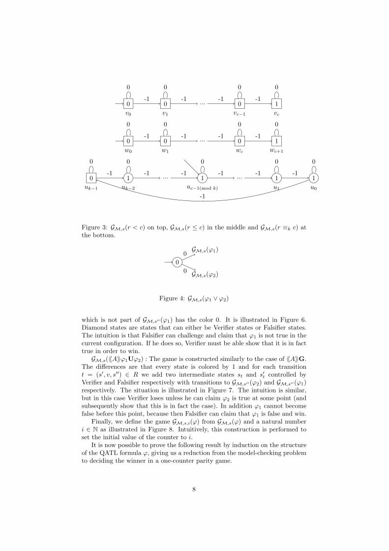
GM,s(r ./ c) : Using negation and conjunction we can define (r = c) ≡ (r ≤c ∧ ¬(r < c)), (r > c) ≡ (¬(r ≤ c)) and (r ≥ c) ≡ (¬(r < c)) and therefore onlyneed to construct games for the cases r < c, r ≤ c and r ≡k c. The three casesare shown in Figure 3.GM,s(ϕ1 ∨ ϕ2) : The game is shown in Figure 4.GM,s(¬ϕ1) : The game is constructed from GM,s(ϕ1) by interchanging circle

states and square states and either adding or subtracting 1 to/from all colors.GM,s(〈〈A〉〉Xϕ1) : Let R(s) = {(s, v, s′) ∈ R} = {(s, v1, s1), ..., (s, vm, sm)}.

There are two cases to consider. One when s ∈ Sj for some j ∈ A and one whens 6∈ Sj for all j ∈ A. Both are illustrated in Figure 5.GM,s(〈〈A〉〉Gϕ1) : In this case we let GM,s(〈〈A〉〉Gϕ1) have the same structure

as M, but with a few differences. Verifier controls all states that are in Sj forsome j ∈ A and Falsifier controls the other states. Further, for each transitiont = (s′, v, s′′) ∈ R we put an intermediate state st controlled by Falsifier betweens′ and s′′. When the player controlling s′ chooses to take the transition tthe play is taken to the intermediate state st from which Falsifier can eitherchoose to continue to s′′ or to go to GM,s′′(ϕ1). Every state in GM,s(〈〈A〉〉Gϕ1)

7

0

v0

0

v1

... 0

vc−1

1

vc

0

w0

0

w1

... 0

wc

1

wc+1

0

uk−1

1

uk−2

... 1

uc−1(mod k)

... 1

u1

1

u0

0 0 0 0

-1 -1 -1 -1

0 0 0 0

-1 -1 -1 -1

0 0 0 0 0

-1 -1 -1 -1 -1 -1

-1

Figure 3: GM,s(r < c) on top, GM,s(r ≤ c) in the middle and GM,s(r ≡k c) atthe bottom.

0

GM,s(ϕ1)

GM,s(ϕ2)

0

0

Figure 4: GM,s(ϕ1 ∨ ϕ2)

which is not part of GM,s′′(ϕ1) has the color 0. It is illustrated in Figure 6.Diamond states are states that can either be Verifier states or Falsifier states.The intuition is that Falsifier can challenge and claim that ϕ1 is not true in thecurrent configuration. If he does so, Verifier must be able show that it is in facttrue in order to win.GM,s(〈〈A〉〉ϕ1Uϕ2) : The game is constructed similarly to the case of 〈〈A〉〉G.

The differences are that every state is colored by 1 and for each transitiont = (s′, v, s′′) ∈ R we add two intermediate states st and s′t controlled byVerifier and Falsifier respectively with transitions to GM,s′′(ϕ2) and GM,s′′(ϕ1)respectively. The situation is illustrated in Figure 7. The intuition is similar,but in this case Verifier loses unless he can claim ϕ2 is true at some point (andsubsequently show that this is in fact the case). In addition ϕ1 cannot becomefalse before this point, because then Falsifier can claim that ϕ1 is false and win.

Finally, we define the game GM,s,i(ϕ) from GM,s(ϕ) and a natural numberi ∈ N as illustrated in Figure 8. Intuitively, this construction is performed toset the initial value of the counter to i.

It is now possible to prove the following result by induction on the structureof the QATL formula ϕ, giving us a reduction from the model-checking problemto deciding the winner in a one-counter parity game.

8

0

GM,s1(ϕ1)

GM,sm(ϕ1)

...v1

vm

0

GM,s1(ϕ1)

GM,sm(ϕ1)

...v1

vm

Figure 5: GM,s(〈〈A〉〉Xϕ1). The case on the left is when s ∈ Sj for some j ∈ Aand the case on the right is when s 6∈ Sj for all j ∈ A

s′ s′′0

s′0st

0

s′′

GM,s′′(ϕ1)

v v 0

0

Figure 6: GM,s(〈〈A〉〉Gϕ1) is obtained by updating each transition in M asshown in the figure.

Proposition 3. For every OCGM M, state s in M, i ∈ N and ϕ ∈ QATL

M, s, i |= ϕ if and only if Verifier has a winning strategy in GM,s,i(ϕ)

4.2 Complexity

In [6] the selective zero-reachability problem for games on 1-dimensional vectoraddition systems with states was shown to be PSpace-complete. This prob-lem consists of model-checking the fixed QATL formula 〈〈{I}〉〉F(r = 0 ∧ p) in a2-player OCGM where I is one of the players. The hardness is shown by a reduc-tion from the emptiness problem of 1-letter alternating finite automata which isPSpace-complete [16]. Thus, the data complexity of model-checking QATL inOCGMs is PSpace-hard. As a consequence of Proposition 3 and Proposition2 this lower bound is tight since we can transform the model-checking problemof QATL to deciding the winner in an OCG with a parity condition that haspolynomial size. Thus, model-checking can be performed in polynomial space.

Theorem 4. The combined complexity and data complexity of model-checkingQATL OCGMs are both PSpace-complete

In [14] it was shown that the data complexity of model-checking CTL inSOCPs is ExpSpace-complete even for a fixed (but rather complicated) for-mula. Since this problem is subsumed by the model-checking problem of QATLin SOCGMs we have the same lower bound for the data complexity of model-checking QATL in SOCGMs. It can be shown that this bound is tight as follows.We can create a model-checking game for QATL in SOCGMs in the same way asfor OCGMs and obtain a model-checking game which is an SOCG with a paritywinning condition. This can be transformed into an OCG with a parity winningcondition that is exponentially larger. It is done by replacing each transitionwith weight v with a path that has v transitions and adding small gadgets tomake sure that a player loses if he tries to take a transition with value −w for

9

s′ s′′1

s′1st

1s′t

1

s′′

GM,s′′(ϕ2) GM,s′′(ϕ1)

v v 0 0

0 0

Figure 7: GM,s(〈〈A〉〉ϕ1Uϕ2) is obtained by updating each transition in M asshown in the figure.

0

v0

0

v1

... 0

vi−1

GM,s(ϕ)1 1 1 1

Figure 8: GM,s,i(ϕ) is obtained by increasing the counter value to i initially.

w ∈ N when the current counter value is less than w. The exponential blowupis due to the weights being input in binary. We can then apply Proposition 2and solve this game in exponential space. Thus, we have the following.

Theorem 5. The combined complexity and data complexity of model-checkingQATL in SOCGMs are both ExpSpace-complete.

These results are quite positive. Indeed, in OCGMs reachability games arealready PSpace-complete [6]. Considering that in QATL we have nesting ofstrategic operators, eventuality operators, safety operators and comparison ofcounter values with constants it is very positive that we stay in the same com-plexity class. For SOCGMs CTL model-checking is already ExpSpace-complete[14] which means that we can add several players as well as counter constraintswithout leaving ExpSpace.

5 Model-checking QATL∗

As for model-checking of QATL we rely on the approach of a model-checkinggame when model-checking QATL∗. However, due to the extended possibilitiesof nesting we do not handle temporal operators directly as we did for formulasof the form 〈〈A〉〉ϕUψ, 〈〈A〉〉Gϕ and 〈〈A〉〉Xϕ. Instead, we resort to a translationof LTL formulas into deterministic parity automata (DPA) which is combinedwith the model-checking game approach. This gives us model-checking gameswhich are one-counter parity games as for QATL, but with doubly exponentialsize in the input formula due to the translation from LTL formulas to DPAs.

5.1 Adjusting the model-checking game to QATL∗

Let M = (S,Π, (Sj)j∈Π, R,AP,L) be an OCGM, s0 ∈ S, i ∈ N and ϕ be aQATL∗ state formula. The algorithm to decide whether M, s0, i |= ϕ followsalong the same lines as our algorithm for QATL. That is, we construct a model-checking game GM,s0,i(ϕ) between two players Verifier and Falsifier that try toverify and falsify the formula respectively. Then Verifier has a winning strategy

10

in GM,s0,i(ϕ) if and only if M, s0, i |= ϕ. The construction is done inductivelyon the structure of ϕ. For each state s ∈ S and state formula ϕ we define acharacteristic OCG GM,s(ϕ). For formulas of the form p, r ./ c,¬ϕ1 and ϕ1∨ϕ2

the construction is as for QATL assuming in the inductive cases that GM,s(ϕ1)and GM,s(ϕ2) have already been defined.

The interesting case is ϕ = 〈〈A〉〉ϕ1. Here, let ψ1, ..., ψm be the outermostproper state subformulas of ϕ1. Let P = {p1, ..., pm} be fresh propositions andlet f(ϕ1) = ϕ1[ψ1 7→ p1, ..., ψm 7→ pm] be the formula obtained from ϕ1 byreplacing the outermost proper state subformulas with the corresponding freshpropositions. Let AP′ = AP ∪ P . Now, f(ϕ1) is an LTL formula over AP′.We can therefore construct a deterministic parity automaton (DPA) Af(ϕ1)

with input alphabet 2AP′such that the language L(Af(ϕ1)) of the automaton is

exactly the set of linear models of f(ϕ1). The number of states of the DPA canbe bounded by O((2n·2

n

)(2n)!) and the number of colors by O(2 ·2n) = O(2n+1)where n is the size of the formula f(ϕ1). These bounds are obtained by usingthe fact that a non-deterministic Buchi automaton (NBA) Bf(ϕ1) with O(2n)states and L(Bf(ϕ1)) = Traces(f(ϕ1)) can be constructed [28]. From this, aDPA accepting the same language can be constructed using a technique from[21] which translates an NBA with m states to a DPA with 2mm ·m! states and2m colors.

The game GM,s(ϕ) is now constructed with the same structure asM, whereVerifier controls the states for players in A and Falsifier controls the states forplayers in Π \ A. However, we need to deal with truth values of the formulasψ1, ..., ψm which can in general not be labelled to states inM since they dependboth on the current state and counter value. Therefore we change the structureto obtain GM,s(ϕ) as follows. For each state s and t with (s, t) ∈ R we embed a

module as shown in Figure 9. Here, 2AP′= {Φ0, ...,Φ`} and for each 0 ≤ j ≤ `

we let {ψj0, ..., ψjkj} = {ψi | pi ∈ Φj} ∪ {¬ψi | pi 6∈ Φj}.

s t s

t(Φ0)

...

t(Φ`)

t

GM,t(ψ00)

...

GM,t(ψ0k0)

GM,t(ψ`0)

...

GM,t(ψ`k`)

v v

0

0

0

0

0

0

0

0

Figure 9: GM,s(〈〈A〉〉ϕ) is obtained by updating each transition as shown in thefigure.

The idea is that when a transition is taken from (s, w) to (t, w+ v), Verifiermust specify which of the propositions p1, ..., pm are true in (t, w+v), this is doneby picking one of the subsets Φj (which is the set of propositions that are true instate t(Φj)). Then, to make sure that Verifier does not cheat, Falsifier has theopportunity to challenge any of the truth values of the propositions specified by

11

Verifier. If Falsifier challenges, the play never returns again. Thus, if Falsifierchallenges incorrectly, Verifier can make sure to win the game. However, ifFalsifier challenges correctly then Falsifier can be sure to win the game. IfVerifier has a winning strategy, then it consists in choosing the correct values ofthe propositions at each step. If Verifier does choose correctly and Falsifier neverchallenges, the winner of the game should be determined based on whether theLTL property specified by f(ϕ1) is satisfied during the play. We handle this bylabelling t(Φj) with the propositions in Φj . Further, since every step of the gameis divided into three steps (the original step, the specification by Verifier and thechallenge opportunity for Falsifier) we alter the deterministc automaton Af(ϕ1)

such that it only takes a transition every third step. This simply increases itssize by a factor 3. We then perform a product of the game with the updatedparity automaton to obtain the parity game GM,s(〈〈A〉〉ϕ1). It is important tonote that the product with the automaton is not performed on the challengemodules (which are already colored), but only with states in the main module.This keeps the size of the game double-exponential in the size of the formula.We now have the following.

Proposition 6. For every OCGM M, state s in M, i ∈ N and state formulaϕ ∈ QATL∗

M, s, i |= ϕ if and only if Verifier has a winning strategy in GM,s,i(ϕ)

Proof. Due to space limitations, we only provide a sketch of the proof with themain ideas. The proof is done by induction on the structure of ϕ. The basecases as well as boolean combinations are omitted since they work as for QATL.The interesting case is ϕ = 〈〈A〉〉ϕ1.

Suppose first thatM, s, i |= 〈〈A〉〉ϕ1. Then coalition A has a winning strategyσ inM. From this, we generate a strategy σ′ for Verifier in GM,s,i(〈〈A〉〉ϕ1) thatconsists in never cheating when specifying values of atomic formulas and choos-ing transitions according to what σ would have done in M. Then, if Falsifierchallenges at some point, Verifier can be sure to win by the induction hypoth-esis since he never cheats. If Falsifier never challenges (or, until he challenges),Verifier simply mimics the collective winning strategy σ of coalition A in Mfrom (s, i). This ensures that he wins in the parity game due to the definitionof the parity condition from the parity automaton corresponding to f(ϕ1).

Suppose on the other hand that Verifier has a winning strategy σ in GM,s,i(〈〈A〉〉ϕ1).Then σ never cheats when specifying values of propositions, because then Falsifiercould win according to the induction hypothesis. Define a strategy σ′ for coali-tion A in M that plays like σ in the part of GM,s,i(〈〈A〉〉ϕ1) where no challengehas occured. σ′ is winning for A with condition ϕ1 in M due to the definitionof GM,s,i(〈〈A〉〉ϕ1) using the automaton Af(ϕ1).

5.2 Complexity

The size of the model-checking game is doubly-exponential in the size of theformula. Therefore, it can be solved in doubly-exponential space because it is aone-counter parity game using Proposition 2. Actually, this is the case for bothOCGMs and SOCGMs. Indeed, we extend the technique to SOCGMs as we didin the case of QATL. However, with respect to complexity, the blowup caused

12

by the binary representation of edge weights only matters when the formula isfixed since the game is already doubly-exponential when the input formula is aparameter. Thus, for QATL∗ we can do model-checking in doubly-exponentialspace whereas for a fixed formula it is in ExpSpace for SOCGMs and PSpacefor OCGMs.

For combined complexity we can show that 2ExpSpace is a tight lowerbound by a reduction from the word acceptance problem of a doubly-exponentialspace Turing machine. The reduction reuses ideas from [16], [17] and [5]. Theproof is in Appendix B. For a fixed formula we get tight lower bounds immedi-ately from the results on QATL.

Theorem 7. The combined complexity of model-checking QATL∗ is 2ExpSpace-complete for both OCGMs and SOCGMs. The data complexity of model-checkingQATL∗ is PSpace-complete for OCGMs and ExpSpace-complete for SOCGMs.

Since we have an ExpSpace lower bound for data complexity of CTL model-checking in SOCPs [14] and a PSpace lower bound for data complexity of CTLmodel-checking in OCPs [15] we get the following results for data complexity ofmodel-checking CTL∗ in OCPs.

Corollary 8. The data complexity of model-checking CTL∗ in OCPs and SOCPsare PSpace-complete and ExpSpace-complete respectively.

Since our lower bound is for formulas of the form 〈〈{I}〉〉ϕ where ϕ is an LTLformula and I is a player we also have the following.

Corollary 9. Deciding the winner in two-player OCGs and SOCGs with LTLobjectives are both 2ExpSpace-complete.

6 Concluding remarks

We have characterized the complexity of the quantitative alternating-time tem-poral logics QATL and QATL∗ with respect to the format of edge weights aswell as whether the input formula is fixed or not. The results are collected inTable 1. Note that all complexity results on QATL and QATL∗ hold for ATLand ATL∗ as well since no counter constraints are used in the proofs of the lowerbounds. As a byproduct we have also obtained results for CTL∗ model-checkingon OCPs. These, along with CTL model-checking results on OCPs and SOCPsfrom the litterature, are included as a comparison.

Given that one-counter reachability games are already PSpace-complete[6] it is very positive that we can extend to QATL model-checking and evento model-checking of fixed QATL∗ formulas without leaving PSpace. Model-checking CTL in SOCPs is already ExpSpace-complete [14] so it is also verypositive that we can extend this to model-checking of QATL and fixed formulasof QATL∗ in succinct one-counter games. Finally, the 2ExpSpace-completenessresults are not too unexpteced compared to the known 2ExpTime lower boundfrom the synthesis of LTL [23] and 3ExpTime-completeness of pushdown gameswith LTL objectives [19]. However, though we restrict to a unary stack alphabetcompared to pushdown games, we do have counter constraints and nesting ofstrategic operators.

Finally, the model-checking game approach has turned out to be quite flexi-ble with respect to enriching the alternating-time temporal logics with counter

13

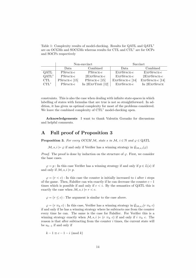
Table 1: Complexity results of model-checking. Results for QATL and QATL∗

are on OCGMs and SOCGMs whereas results for CTL and CTL∗ are for OCPsand SOCPs respectively

Non-succinct SuccinctData Combined Data Combined

QATL PSpace-c PSpace-c ExpSpace-c ExpSpace-cQATL∗ PSpace-c 2ExpSpace-c ExpSpace-c 2ExpSpace-cCTL PSpace-c [15] PSpace-c [15] ExpSpace-c [14] ExpSpace-c [14]CTL∗ PSpace-c In 2ExpTime [12] ExpSpace-c In 2ExpSpace

constraints. This is also the case when dealing with infinite state-spaces in whichlabelling of states with formulas that are true is not so straightforward. In ad-dition, it has given us optimal complexity for most of the problems considered.We leave the combined complexity of CTL∗ model-checking open.

Acknowledgements I want to thank Valentin Goranko for discussionsand helpful comments.

A Full proof of Proposition 3

Proposition 3. For every OCGM M, state s in M, i ∈ N and ϕ ∈ QATL

M, s, i |= ϕ if and only if Verifier has a winning strategy in GM,s,i(ϕ)

Proof. The proof is done by induction on the structure of ϕ. First, we considerthe base cases.

ϕ = p : In this case Verifier has a winning strategy if and only if p ∈ L(s) ifand only if M, s, i |= p.

ϕ = (r < c) : In this case the counter is initially increased to i after i stepsof the game. Then, Falsifier can win exactly if he can decrease the counter c−1times which is possible if and only if c < i. By the semantics of QATL this isexactly the case when M, s, i |= r < c.

ϕ = (r ≤ c) : The argument is similar to the case above.

ϕ = (r ≡k c) : In this case, Verifier has a winning strategy in GM,s,i(r ≡k c)if and only if he has a winning strategy where he subtracts one from the counterevery time he can. The same is the case for Falsifier. For Verifier this is awinning strategy exactly when M, s, i |= (r ≡k c) if and only if i ≡k c. Thereason is that after subtracting from the counter i times, the current state willbe uk−1 if and only if

k − 1 ≡ c− 1− i (mod k)

14

⇔ k ≡ c− i (mod k)

⇔ i ≡ c (mod k)⇔ i ≡k c

Next, we consider the inductive cases.

ϕ = ϕ1 ∨ ϕ2 : Clearly, if Verifier has a winning strategy in GM,s,i(ϕ1) or inGM,s,i(ϕ2) then he has a winning strategy in GM,s,i(ϕ1∨ϕ2) since he can choosewhich of the games to play and reuse the winning strategy. On other hand, ifVerifier has a winning strategy in GM,s,i(ϕ1 ∨ ϕ2) then he is either winning inGM,s,i(ϕ1) or in GM,s,i(ϕ2) because he can reuse the strategy and be sure towin in at least one of these games. Then, by using the induction hypothesis wehave that Verifier has a winning strategy in GM,s,i(ϕ1∨ϕ2) if and only if he hasa winning strategy in GM,s,i(ϕ1) or in GM,s,i(ϕ2) if and only if M, s, i |= ϕ1 orM, s, i |= ϕ2 if and only if M, s, i |= ϕ1 ∨ ϕ2.

ϕ = ¬ϕ1 : The construction essentially switches Verifier with Falsifier whencreating GM,s,i(¬ϕ1) from GM,s,i(ϕ1). This means that Verifier has a win-ning strategy in GM,s,i(¬ϕ1) if and only if Falsifier has a winning strategy inGM,s,i(ϕ1). As a consequence of the determinacy result for Borel games [20]we have that one-counter games with parity conditions are determined. It fol-lows that Verifier has a winning strategy in GM,s,i(¬ϕ1) if and only if Verifierdoes not have a winning strategy in GM,s,i(ϕ1). Using the induction hypothesisthis means that Verifier has a winning strategy in GM,s,i(¬ϕ1) if and only ifM, s, i 6|= ϕ1 if and only if M, s, i |= ¬ϕ1.

ϕ = 〈〈A〉〉Xϕ1 : There are two cases to consider. First, suppose s ∈ Sj forsome j ∈ A. Then Verifier has a winning strategy in GM,s,i(〈〈A〉〉Xϕ1) if andonly if there is a transition (s, v, s′) ∈ R with v + i ≥ 0 such that Verifier hasa winning strategy in GM,s′,i+v(ϕ1) since parity objectives are prefix indepen-dent. Using the induction hypothesis, this is the case if and only if there is atransition (s, v, s′) ∈ R with v + i ≥ 0 such that M, s′, i+ v |= ϕ1 which is thecase if and only if M, s, i |= 〈〈A〉〉Xϕ1. For the case where s 6∈ Sj for all j ∈ Athe proof is similar, but uses universal quantification over the transitions.

ϕ = 〈〈A〉〉Gϕ1 : The intuition of the construction is that Verifier controls theplayers in A and Falsifier controls the players in Π \ A. At each configuration(s′, v) ∈ S × N of the game Falsifier can challenge the truth value of ϕ1 bygoing to GM,s′,v(ϕ1) in which Falsifier has a winning strategy if and only if ϕ1

is indeed false in M, s′, v. If Falsifier challenges at the wrong time or neverchallenges then Verifier can make sure to win.

More precisely, suppose Verifier has a winning strategy σ in GM,s,i(〈〈A〉〉Gϕ1)then every possible play when Verifier plays according to σ either never goesinto one of the modules GM,s′(ϕ1) or the play goes into one of the modulesat some point and never returns. Since σ is a winning strategy for I, we haveby the induction hypothesis that every pair (s′, v) ∈ S × N reachable whenVerifier plays according to σ is such that M, s′, v |= ϕ1, because otherwise σwould not be a winning strategy for I. If coalition A follows the same strategyσ adapted to M then the same state, value pairs are reachable. Since for allthese reachable pairs (s′, v) we have M, s′, v |= ϕ1 this strategy is a witness

15

that M, s, i |= 〈〈A〉〉Gϕ1.On the other hand, suppose that coalition A can ensure Gϕ1 from (s, i) using

strategy σ. Then in every reachable configuration (s′, v) we haveM, s′, v |= ϕ1.From this we can generate a winning strategy for Verifier in GM,s,i(〈〈A〉〉Gϕ1)that plays in the same way until (if ever) Falsifier challenges and takes a tran-sition to a module GM,s′,v(ϕ1) for some (s′, v). Since the same configurationscan be reached before a challenge as when A plays according to σ, this meansthat Verifier can make sure to win in GM,s′,v(ϕ1) by the induction hypothesis.Thus, if Falsifier challenges Verifier can make sure to win and if Falsifier neverchallenges Verifier also wins since all states reached have color 0. Thus, Verifierhas a winning strategy in GM,s,i(〈〈A〉〉Gϕ1).

ϕ = 〈〈A〉〉ϕ1Uϕ2 : The proof works as the case above with some minordifferences. In this case, Verifier needs to show that he can reach a configurationwhere ϕ2 is true when controlling the players in A and therefore he loses if hecan never reach a module GM,s′,v(ϕ2) such that M, s′, v |= ϕ2. At the sametime, he has to make sure that configurations (s′, v) where M, s′, v 6|= ϕ1 arenot reached in an intermediate configuration since Falsifier still has the abilityto challenge, as in the previous case. Note that Verifier gets the chance tocommit to showing that ϕ2 is true in a given configuration before Falsifier getsthe change to challenge the value of ϕ1. This is due to the definition of the untiloperator that does not require ϕ1 to be true at the point where ϕ2 becomestrue. We leave out the remaining details.

B Full proof of Theorem 7

We will show that model-checking ATL∗ in OCGMs is 2ExpSpace-hard bya reduction from the word acceptance problem for a deterministic doubly-exponential space Turing machine. From this, the theorem follows from theobservations in the main text.

Let T = (Q, q0,Σ, δ, qF ) be a deterministic Turing machine that uses at

most 22|w|k

tape cells on input w where k is a constant and |w| is the number ofsymbols in w. Here, Q is a finite set of control states, q0 ∈ Q is the initial controlstate. Σ = {0, 1,#, a, r} is the tape alphabet containing the blank symbol #and special symbols a and r such that T accepts immediately if it reads a andrejects immediately if it reads r, δ : Q × Σ → Q × Σ × {Left,Right} is thetransition function and qF ∈ Q is the accepting state. If δ(q, a) = (q′, a′, x) wewrite δ1(q, a) = q′, δ2(q, a) = a′ and δ3(q, a) = x. Let ΣI = Σ \ {#}. Now, letw = w1...w|w| ∈ Σ∗I be an input word. From this we construct an OCGM M,

an initial state s0 and a QATL∗ formula Φ all with size polynomial in n = |w|kand |T | such that T accepts w if and only if M, (s0, 0) |= Φ.

We use an intermediate step in the reduction for simplicity of the arguments.This is done by considering an OCG G = (S′, {Verifier,Falsifier}, (S′Verifier, S

′Falsifier), R

′)with two players Verifier and Falsifier and an initial state s′0 such that Verifiercan force the play to reach s′F if and only if T accepts w. However, the size ofthe set S′ of states will be doubly-exponential in n. The idea of this constructionresembles a reduction from the word acceptance problem for polynomial-spaceTuring machines to the emptiness problem for alternating finite automata with

16

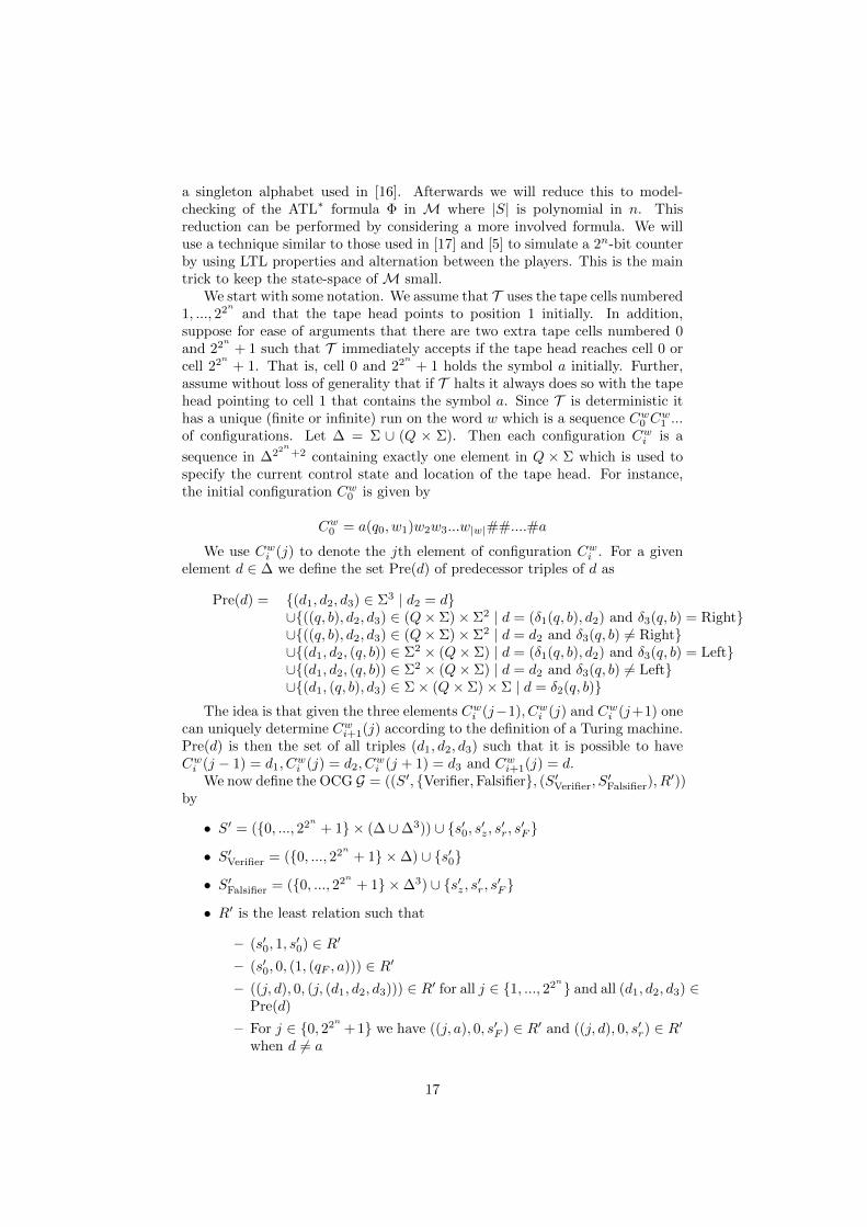
a singleton alphabet used in [16]. Afterwards we will reduce this to model-checking of the ATL∗ formula Φ in M where |S| is polynomial in n. Thisreduction can be performed by considering a more involved formula. We willuse a technique similar to those used in [17] and [5] to simulate a 2n-bit counterby using LTL properties and alternation between the players. This is the maintrick to keep the state-space of M small.

We start with some notation. We assume that T uses the tape cells numbered1, ..., 22n

and that the tape head points to position 1 initially. In addition,suppose for ease of arguments that there are two extra tape cells numbered 0and 22n

+ 1 such that T immediately accepts if the tape head reaches cell 0 orcell 22n

+ 1. That is, cell 0 and 22n

+ 1 holds the symbol a initially. Further,assume without loss of generality that if T halts it always does so with the tapehead pointing to cell 1 that contains the symbol a. Since T is deterministic ithas a unique (finite or infinite) run on the word w which is a sequence Cw

0 Cw1 ...

of configurations. Let ∆ = Σ ∪ (Q × Σ). Then each configuration Cwi is a

sequence in ∆22n+2 containing exactly one element in Q × Σ which is used tospecify the current control state and location of the tape head. For instance,the initial configuration Cw

0 is given by

Cw0 = a(q0, w1)w2w3...w|w|##....#a

We use Cwi (j) to denote the jth element of configuration Cw

i . For a givenelement d ∈ ∆ we define the set Pre(d) of predecessor triples of d as

Pre(d) = {(d1, d2, d3) ∈ Σ3 | d2 = d}∪{((q, b), d2, d3) ∈ (Q× Σ)× Σ2 | d = (δ1(q, b), d2) and δ3(q, b) = Right}∪{((q, b), d2, d3) ∈ (Q× Σ)× Σ2 | d = d2 and δ3(q, b) 6= Right}∪{(d1, d2, (q, b)) ∈ Σ2 × (Q× Σ) | d = (δ1(q, b), d2) and δ3(q, b) = Left}∪{(d1, d2, (q, b)) ∈ Σ2 × (Q× Σ) | d = d2 and δ3(q, b) 6= Left}∪{(d1, (q, b), d3) ∈ Σ× (Q× Σ)× Σ | d = δ2(q, b)}

The idea is that given the three elements Cwi (j−1), Cw

i (j) and Cwi (j+1) one

can uniquely determine Cwi+1(j) according to the definition of a Turing machine.

Pre(d) is then the set of all triples (d1, d2, d3) such that it is possible to haveCw

i (j − 1) = d1, Cwi (j) = d2, C

wi (j + 1) = d3 and Cw

i+1(j) = d.We now define the OCG G = ((S′, {Verifier,Falsifier}, (S′Verifier, S

′Falsifier), R

′))by

• S′ = ({0, ..., 22n

+ 1} × (∆ ∪∆3)) ∪ {s′0, s′z, s′r, s′F }

• S′Verifier = ({0, ..., 22n

+ 1} ×∆) ∪ {s′0}

• S′Falsifier = ({0, ..., 22n

+ 1} ×∆3) ∪ {s′z, s′r, s′F }

• R′ is the least relation such that

– (s′0, 1, s′0) ∈ R′

– (s′0, 0, (1, (qF , a))) ∈ R′

– ((j, d), 0, (j, (d1, d2, d3))) ∈ R′ for all j ∈ {1, ..., 22n} and all (d1, d2, d3) ∈Pre(d)

– For j ∈ {0, 22n

+1} we have ((j, a), 0, s′F ) ∈ R′ and ((j, d), 0, s′r) ∈ R′when d 6= a

17

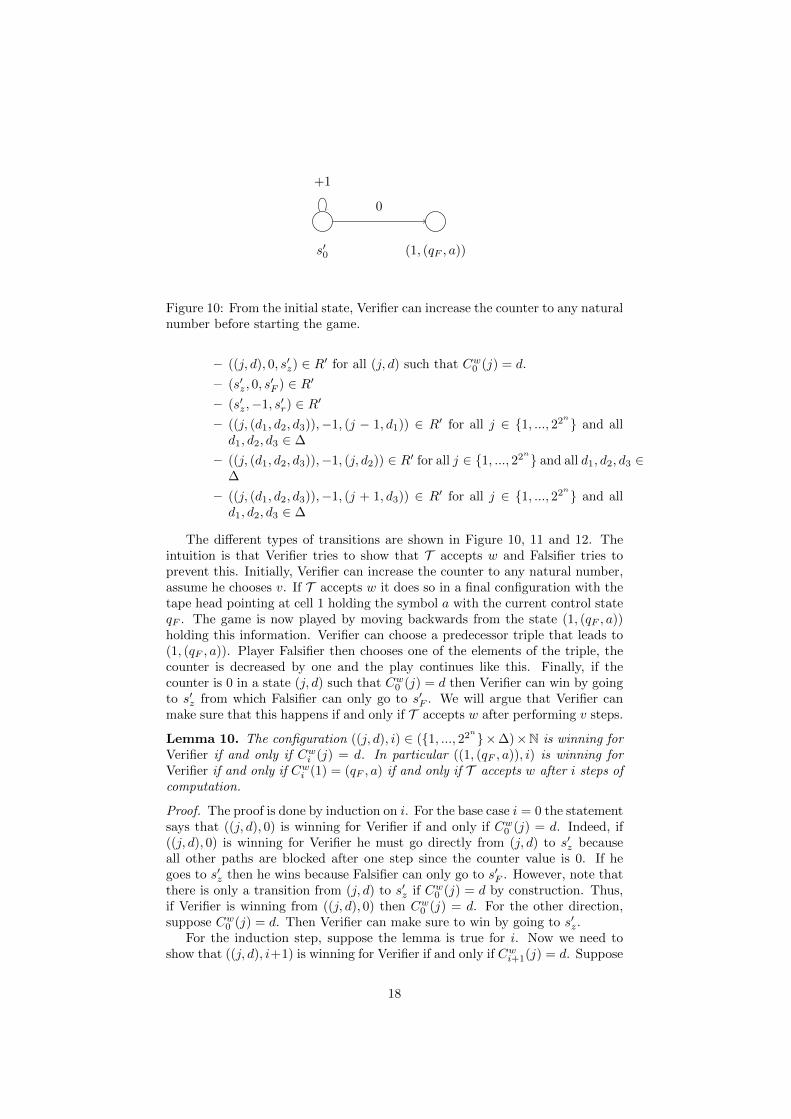
s′0 (1, (qF , a))

+1

0

Figure 10: From the initial state, Verifier can increase the counter to any naturalnumber before starting the game.

– ((j, d), 0, s′z) ∈ R′ for all (j, d) such that Cw0 (j) = d.

– (s′z, 0, s′F ) ∈ R′

– (s′z,−1, s′r) ∈ R′

– ((j, (d1, d2, d3)),−1, (j − 1, d1)) ∈ R′ for all j ∈ {1, ..., 22n} and alld1, d2, d3 ∈ ∆

– ((j, (d1, d2, d3)),−1, (j, d2)) ∈ R′ for all j ∈ {1, ..., 22n} and all d1, d2, d3 ∈∆

– ((j, (d1, d2, d3)),−1, (j + 1, d3)) ∈ R′ for all j ∈ {1, ..., 22n} and alld1, d2, d3 ∈ ∆

The different types of transitions are shown in Figure 10, 11 and 12. Theintuition is that Verifier tries to show that T accepts w and Falsifier tries toprevent this. Initially, Verifier can increase the counter to any natural number,assume he chooses v. If T accepts w it does so in a final configuration with thetape head pointing at cell 1 holding the symbol a with the current control stateqF . The game is now played by moving backwards from the state (1, (qF , a))holding this information. Verifier can choose a predecessor triple that leads to(1, (qF , a)). Player Falsifier then chooses one of the elements of the triple, thecounter is decreased by one and the play continues like this. Finally, if thecounter is 0 in a state (j, d) such that Cw

0 (j) = d then Verifier can win by goingto s′z from which Falsifier can only go to s′F . We will argue that Verifier canmake sure that this happens if and only if T accepts w after performing v steps.

Lemma 10. The configuration ((j, d), i) ∈ ({1, ..., 22n}×∆)×N is winning forVerifier if and only if Cw

i (j) = d. In particular ((1, (qF , a)), i) is winning forVerifier if and only if Cw

i (1) = (qF , a) if and only if T accepts w after i steps ofcomputation.

Proof. The proof is done by induction on i. For the base case i = 0 the statementsays that ((j, d), 0) is winning for Verifier if and only if Cw

0 (j) = d. Indeed, if((j, d), 0) is winning for Verifier he must go directly from (j, d) to s′z becauseall other paths are blocked after one step since the counter value is 0. If hegoes to s′z then he wins because Falsifier can only go to s′F . However, note thatthere is only a transition from (j, d) to s′z if Cw

0 (j) = d by construction. Thus,if Verifier is winning from ((j, d), 0) then Cw

0 (j) = d. For the other direction,suppose Cw

0 (j) = d. Then Verifier can make sure to win by going to s′z.For the induction step, suppose the lemma is true for i. Now we need to

show that ((j, d), i+1) is winning for Verifier if and only if Cwi+1(j) = d. Suppose

18

(j, d)

(j, (d11, d12, d13))

...

(j, (d|Pre(d)|1, d|Pre(d)|2, d|Pre(d)|3))

s′z

s′F s′r

0

0

00

0 -1

Figure 11: From a state (j, d) ∈ {1, ..., 22n}×∆ Verifier can choose a predecessortriple of d. The dashed transition is enabled only when Cw

0 (j) = d. In this caseVerifier can be sure to win if the current counter value is 0.

(j, (d1, d2, d3))

(j − 1, d1)

(j, d2)

(j + 1, d3)

-1

-1

-1

Figure 12: From a precedessor triple chosen by Verifier, Falsifier can choosewhich predecessor to continue with.

19

first that ((j, d), i + 1) is winning for Verifier. The winning strategy σ cannotconsist in going directly to s′z because then Falsifier can go to s′r. Thus, Verifiermust choose a predecessor triple (d1, d2, d3) ∈ Pre(d) when playing accordingto σ. After he chooses this, Falsifier chooses one of them and the counter isdecreased by one. Thus, Falsifier can choose either ((j − 1, d1), i), ((j, d2), i) or(j+1, d3), i). Thus, by the induction hypothesis Cw

i (j−1) = d1, Cwi (j) = d2 and

Cwi (j+1) = d3 since Verifier is winning. By the definition of predecessor triples,

this means that Cwi+1(j) = d. For the other direction, suppose Cw

i+1(j) = d.Then by going to the state (j, (Cw

i (j − 1), Cwi (j), Cw

i (j + 1))) he can be sure towin by the induction hypothesis.

Lemma 11. Starting in configuration (s′0, 0) Verifier can make sure to reachs′F if and only if T accepts w.

We have now reduced the word acceptance problem to a reachability gamein an OCG G with a doubly-exponential number of states. Due to the structureof G we can reduce this to model-checking the ATL∗ formula Φ in the OCGMM. The difficult part is that we need to store the number of the tape cellthat the tape head is pointing at, which can be of doubly-exponential size. Theother features of G are polynomial in the input. Note that at each step of thegame, the position of the tape head either stays the same, increases by one ordecreases by one. This is essential for our ability to encode it using ATL∗. WeconstructM much like G but where the position of the tape head is not presentin the set of states. Instead, for each transition in the game between states sand s′ we have a module in which Verifier encodes the position of the tape headby his choices. At the same time, Falsifier has the possibility to challenge ifVerifier has not chosen the correct value of the tape head position. This canbe ensured by use of the ATL∗ formula Φ = 〈〈{Verifier}〉〉ϕ where ϕ is an LTLformula. The details of simulating a 2n-bit counter like this can be obtainedfrom [17, 5]. According to the choices of Falsifier then Verifier must be ableto increase, decrease or leave unchanged the position of the tape head. Thiscan be enforced by a formula with a size polynomial in n. Except for havingto implement the position of the tape head in this way, the rules of M are thesame as for G where Verifier needs to show that T accepts w by choosing astrategy that ensures reaching a certain state in the game while updating thetape head position correctly. In the end, this means that for the initial state s0

in M corresponding to s′0 in G we get M, s0, 0 |= 〈〈{Verifier}〉〉(ϕ ∧ FsF ) if andonly if T halts on w. Here we assume that the play also goes to a halting statesF corresponding to s′F if Falsifier challenges the counter value incorrectly.

Theorem 7. The combined complexity of model-checking QATL∗ is 2ExpSpace-complete for both OCGMs and SOCGMs. The data complexity of model-checkingQATL∗ is PSpace-complete for OCGMs and ExpSpace-complete for SOCGMs.

References

[1] Rajeev Alur, Thomas A. Henzinger, and Orna Kupferman. Alternating-time temporal logic. J. ACM, 49(5):672–713, 2002.

20

[2] Aaron Bohy, Veronique Bruyere, Emmanuel Filiot, and Jean-FrancoisRaskin. Synthesis from ltl specifications with mean-payoff objectives. InTACAS, pages 169–184, 2013.

[3] Patricia Bouyer, Ulrich Fahrenberg, Kim Guldstrand Larsen, NicolasMarkey, and Jirı Srba. Infinite runs in weighted timed automata withenergy constraints. In FORMATS, pages 33–47, 2008.

[4] Laura Bozzelli. Complexity results on branching-time pushdown modelchecking. Theor. Comput. Sci., 379(1-2):286–297, 2007.

[5] Laura Bozzelli, Aniello Murano, and Adriano Peron. Pushdown modulechecking. In LPAR, pages 504–518, 2005.

[6] Tomas Brazdil, Petr Jancar, and Antonın Kucera. Reachability games onextended vector addition systems with states. In ICALP (2), pages 478–489, 2010.

[7] Nils Bulling and Valentin Goranko. How to be both rich and happy: Com-bining quantitative and qualitative strategic reasoning about multi-playergames (extended abstract). In SR, pages 33–41, 2013.

[8] Krishnendu Chatterjee and Laurent Doyen. Energy parity games. Theor.Comput. Sci., 458:49–60, 2012.

[9] Edmund M. Clarke and E. Allen Emerson. Design and synthesis of syn-chronization skeletons using branching-time temporal logic. In Logic ofPrograms, pages 52–71, 1981.

[10] Stephane Demri and Regis Gascon. The effects of bounding syntactic re-sources on presburger ltl. J. Log. Comput., 19(6):1541–1575, 2009.

[11] E. Allen Emerson and Joseph Y. Halpern. “sometimes” and “not never” re-visited: on branching versus linear time temporal logic. J. ACM, 33(1):151–178, 1986.

[12] Javier Esparza, Antonın Kucera, and Stefan Schwoon. Model-checking ltlwith regular valuations for pushdown systems. In TACS, pages 316–339,2001.

[13] Alain Finkel, Bernard Willems, and Pierre Wolper. A direct symbolic ap-proach to model checking pushdown systems. Electr. Notes Theor. Comput.Sci., 9:27–37, 1997.

[14] Stefan Goller, Christoph Haase, Joel Ouaknine, and James Worrell. Modelchecking succinct and parametric one-counter automata. In ICALP (2),pages 575–586, 2010.

[15] Stefan Goller and Markus Lohrey. Branching-time model checking of one-counter processes and timed automata. SIAM J. Comput., 42(3):884–923,2013.

[16] Petr Jancar and Zdenek Sawa. A note on emptiness for alternating finiteautomata with a one-letter alphabet. Inf. Process. Lett., 104(5):164–167,2007.

21

[17] Orna Kupferman, P. Madhusudan, P. S. Thiagarajan, and Moshe Y. Vardi.Open systems in reactive environments: Control and synthesis. In CON-CUR, pages 92–107, 2000.

[18] Orna Kupferman, Moshe Y. Vardi, and Pierre Wolper. Module checking.Inf. Comput., 164(2):322–344, 2001.

[19] Christof Loding, P. Madhusudan, and Olivier Serre. Visibly pushdowngames. In FSTTCS, pages 408–420, 2004.

[20] Donald A. Martin. Borel determinacy. Annals of Mathematics, 102(2):363–371, September 1975.

[21] Nir Piterman. From nondeterministic buchi and streett automata to de-terministic parity automata. Logical Methods in Computer Science, 3(3),2007.

[22] Amir Pnueli. The temporal logic of programs. In FOCS, pages 46–57, 1977.

[23] Amir Pnueli and Roni Rosner. On the synthesis of a reactive module. InPOPL, pages 179–190, 1989.

[24] Amir Pnueli and Roni Rosner. On the synthesis of an asynchronous reactivemodule. In ICALP, pages 652–671, 1989.

[25] Olivier Serre. Parity games played on transition graphs of one-counterprocesses. In FoSSaCS, pages 337–351, 2006.

[26] Moshe Y. Vardi. Reasoning about the past with two-way automata. InICALP, pages 628–641, 1998.

[27] Igor Walukiewicz. Pushdown processes: Games and model-checking. Inf.Comput., 164(2):234–263, 2001.

[28] Pierre Wolper, Moshe Y. Vardi, and A. Prasad Sistla. Reasoning aboutinfinite computation paths (extended abstract). In FOCS, pages 185–194,1983.

22