modal analysis of rotating wind turbine using multiblade
TRANSCRIPT

Modal Analysis of Rotating Wind Turbine using Multiblade Coordinate Transformation
and Harmonic Power Spectrum
Shifei Yang [email protected]
Department of Engineering Physics University of Wisconsin-Madison
Dmitri Tcherniak Research Engineer
[email protected] Brüel & Kjær SVM
&
Matthew S. Allen Associate Professor
[email protected] Department of Engineering Physics University of Wisconsin-Madison
Abstract
Understanding and characterization of wind turbine dynamics, especially when operating, is an important
though challenging task. The main problem is that an operating wind turbine cannot be truly modeled as a time
invariant system, which limits the applicability of conventional well-established modal analysis methods. This paper
compares two experimental techniques that characterize the dynamic behavior of an operating horizontal axis wind
turbine (Vestas V27, 225kW, rotor diameter 27m, 12 accelerometers on each blade). The first method uses a
multiblade coordinate transformation to convert the time periodic system into a time invariant one, assuming that the
system is perfectly isotropic. Conventional operational modal analysis then can be applied to identify the modal
parameters of the time invariant model. The second method processes the periodic response directly based on an
extension of modal analysis to linear time periodic systems. It utilizes the harmonic power spectrum, which is
analogous to the power spectrum for a time invariant system, to identify a periodic model for the turbine. This work
demonstrates both of these methods on measurements from the operating turbine and discusses the challenges that
are encountered. The procedure is demonstrated by using it to extract the time-periodic mode shapes of the first
edge-wise modes, revealing that this turbine apparently has non-negligible blade-to-blade variations and hence the
dynamics of these modes are considerably different than one would expect for an anisotropic turbine.

1. Introduction
The design of modern wind turbines heavily relies on accurate numerical models, which are used
extensively to simulate the dynamic behavior of the wind turbines under different operating conditions. As a
consequence, good experimental tools are necessary to validate the numerical models. However, it is quite
challenging to experimentally characterize the dynamics of a wind turbine, especially when it is operating. One
significant challenge is that many real turbines cannot be adequately modeled as a Linear Time Invariant (LTI)
because of blade-to-blade variations, stratification in the flow field, and rotation of the rotor. If the angular speed of
the rotor is constant then a wind turbine might be modeled as a Linear Time Periodic (LTP) system in order to
characterize its behavior. This requires other methods, different from the conventional well-established modal
analysis methods that are normally used for LTI systems.
This paper compares two experimental techniques for identifying wind turbines; the multiblade coordinate
(MBC) transformation and the harmonic power spectrum. The MBC transformation, also known as the Coleman
transformation, was first introduced in [1]. The idea behind the MBC transformation is to substitute the deflections
of the blades measured in the blade coordinate system by some special variables, which combine the deflections of
all three blades. MBC transformation results in elimination of the periodic terms in the equations of motion, thus
making the system time invariant so that conventional modal analysis techniques can be applied. A fundamental
requirement for the MBC transformation is that the rotor is isotropic [2], namely that all blades are identical and
symmetrically mounted on the hub. When focusing on experimental techniques, it is also necessary that
measurement system is symmetric, i.e. the sensors are mounted identically on all three blades [3]. In a prior work,
Tcherniak et al. used the MBC transformation on simulated wind turbine data in order to obtain a wind turbine
Campbell diagram, i.e. a graph presenting the dependency of the modal parameters on the rotor speed [4].
The second method, the harmonic transfer function for linear time periodic systems, was developed to
process the response of the linear time periodic system directly [5]. It is known that when a single frequency input
is applied to an LTI structure, the response will be at the same frequency but with a different phase and amplitude.
In contrast, the response of an LTP system will contain a component at the excitation frequency as well as at an
infinite number of its harmonics, separated by an integer multiple of rotation frequency. The harmonic transfer
function is analogous to the transfer function of a time invariant system, but relates the exponentially modulated
input (i.e., an input signal described by a central frequency and a series of equally spaced harmonics) to the
exponentially modulated output at the same collection of frequencies. Allen et al. extended the harmonic transfer
function to the case where the input cannot be directly measured by introducing the harmonic power spectrum [6],
and the modal parameters of a 5MW turbine were identified from simulated data. Later, the harmonic power
spectrum was combined with continuous-scan laser Doppler vibrometry, measuring the first few mode shapes along
a single blade of a parked 20KW wind turbine under wind excitation [7].
In this work, both the MBC transformation and harmonic power spectrum were employed to process
measurements from an operating turbine under wind excitation. First, the formulation of modes of an LTV system
used in both methods is discussed and compared. Then, the methods are applied to a horizontal axis wind turbine
(Vestas V27, 225kW, rotor diameter 27m), which was instrumented with accelerometers on three blades and in the

nacelle [3]. The identified modal parameters from both methods are discussed and compared to evaluate their
validity. The rest of this paper is organized as follows: Section 2 introduces the theoretical basis for the MBC
transformation and the harmonic power spectrum; Section 3 introduces the wind turbine and sensor arrangement.
Sections 4-6 demonstrate the analysis applied to the data; Section 7 summarizes the paper.
2. Theory
2.1. Multiblade Coordinate Transformation
A multiblade coordinate transformation (MBC) is typically used to convert degrees of freedom (DOFs)
measured on the blades, i.e. in the rotating frame, to a non-rotating frame [8], making it possible to combine the
blade DOFs with those on the tower and the nacelle. In the case of a three-bladed rotor, the sets of three coordinates
{q1,k , q2,k , q3,k}T measured at the position k on blades 1, 2, 3 will be converted to the sets of three multiblade
coordinates {a0,k , a1,k , b1,k}T given by
3 3 3
1 2 20, , 1, , 1, ,3 3 3
1 1 1
, cos , sin ,k i k k i k i k i k ii i i
a q a q b q= = =
= = φ = φ (1)
Where ϕi is the instantaneous azimuth angle of the ith blade, and k = 1…M is a DOF number. The transformation
assumes the blades are evenly distributed, i.e., ϕi = ϕi +2π(i – 1)/3, i = 1, 2, 3. The backward transformation, from
the multiblade coordinates to the blade coordinates is given by
, 0, 1, 1,cos sini k k k i k iq a a b= + φ + φ . (2)
Typically the equation of motion (EoM) is written for a mixture of blade and tower/nacelle DOFs,
0KxxCxM =++ , (3)
with
LMLMM Rssqqqq +Τ ∈= 3
1,31,3,11,1 ,}..,..,..,..{ xx , (4)
where sl, l=1..L are DOF measured in the non-rotating frame. For an operating wind turbine, the mass matrix M,
gyroscopic/damping matrix C and stiffness matrix K are periodic in time: M(t)=M(t+T), C(t)=C(t+T), K(t)=K(t+T),
where T=2π/Ω is a period of the rotor rotation and Ω is its circular frequency. Thus Eq. (3) describes a linear time
periodic (LTP) system, and application of the classical modal approach is impossible since the basic assumption of
the modal decomposition, that the system under test is linear and time invariant, is violated here.
Using Eq. (2) to substitute the coordinates qi,k into Eq. (4), and leaving coordinates sl unchanged, one
arrives at EoM in multiblade coordinates:
0zKzCzM =++ BBB , (5)
where

LMLMMM Rssbaabaa +Τ ∈= 3
1,1,1,01,11,11,0 ,}..,,,...,,{ zz . (6)
Hansen et.al. [2, 9] state that, if the rotor is isotropic, the matrices MB, CB and KB are constant, and thus
MBC transformation converts the LTP system into an LTI system. Bir [8] generally disagrees with this statement
but admits that, under the rotor isotropy assumption, the MBC transformation filters out all periodic terms from the
EoM, except those that are integer multiples of 3Ω. In the same paper, Bir also clarifies some typical misconceptions
regarding MBC, one of them is the necessity of the stationarity of the rotor speed (Ω=const).
In any event, converting the LTP system in Eq. (3) into the LTI system in Eq. (5) allows the application of
the classical modal approach to the new system, i.e., presenting the system dynamics as a superposition of modes,
and finding the corresponding modal parameters: modal frequencies, damping and mode shapes. This paper
concerns output-only modal analysis, i.e., the operating wind turbine is loaded by pure wind and unmeasured forces
due to the rotation of the turbine. Then the obtained mode shapes are transferred back to the blade coordinates using
Eq. (2). In [4], this method was applied to simulated wind turbine data; this paper extends the analysis to the
measured data and compares it with the results from another method, outlined in the next section.
When considering a time variant mechanical system, the term “mode” becomes somehow vague. If an
operating wind turbine with isotropic rotor is described in multiblade coordinates, the system becomes LTI where
the “modes” are well defined. Let us consider a mode of system (5), and assume it has the following modal
parameters: the eigenvalue
2j 1r r r r rλ ζ ω ω ζ= − + − , (7)
where ζr represents the modal damping and ωr is the undamped natural frequency. The corresponding mode shape is
T 30,1 1,1 1,1 0, 1, 1, 1{ , , ... , , , .. } , M L
r M M M L r rψ a a b a a b s s ψ C += ∈ . (8)
The elements of the mode shape vector are complex numbers.
Employing a backward MBC transformation, it is possible to map this mode into the natural blade
coordinates. For rotor angular speed Ω, the motion at the kth DOF on the ith blade corresponding to this mode will be:
)()()()( ,,,, ttttq kikikiki βαγ ++= , (9)
where
( )
( )
j, 0,
2j ( 1)j( )1 3
, 1, 1,2
2j ( 1)j( )1 3
, 1, 1,2
( ) ;
( ) ;
( ) ,
r r r
r r r
r r r
t ti k k
it ti k k k
it ti k k k
t e a
t e a jb e
t e a jb e
ω −ζ ω
π −ω +Ω −ζ ω
π− −ω −Ω −ζ ω
γ =
α = −
β = +
(10)
As one can see, in the blade coordinates the modes of the LTI system in Eq. (5) occur in groups of three,
with frequencies: ωr – Ω, ωr, and ωr + Ω. In general each of these modes could have a different damping ratio, ζr,
although in eq. (10). The γ component does not depend on blade’s number i, meaning that all three blades oscillate

in phase; this is a so-called collective mode. The backward whirling (or anti-symmetric) mode α has a frequency ωr
+ Ω; blade number i+1 lags behind blade number i by –1200. The forward whirling mode β has frequency ωr – Ω;
blade number i+1 lags behind blade number i by +1200.
2.2. Harmonic Power Spectrum of LTP system
A single frequency input to an LTI system causes a response at the same frequency. In contrast, the same
input to an LTP system, e.g., a wind turbine, causes a response that includes the excitation frequency and also an
infinite number of its harmonics. An Exponentially Modulated Periodic (EMP) signal space [5] is defined to contain
the frequency component at the single excitation frequency as well as its harmonics. Specifically, if the frequency of
interest was ω then the EMP signal would consist of a collection of sinuosoids at frequencies ω±nΩ, each having a
different amplitude and phase. The harmonic transfer function is a matrix that relates an EMP input signal
(expressed as a vector of harmonic amplitudes at ω±nΩ) to an EMP output signal. Details about how to derive the
harmonic transfer function and then the harmonic power spectrum can be found in [10].
In practice, one would often like to express a measured signal as an EMP signal, for example in order to
compute transfer functions. This is done by creating several frequency shifted copies of the signal. Specifically,
suppose an output y(t) is measured. An EMP output signal in the frequency domain would be expressed as,
[ ]T
1 0 1( ) ( ) ( ) ( )Y Y Yω ω ω ω−=Y (11)
where Yn(ω) is the FFT of the nth modulated output signal yn(t),
j( ) ( ) n tny t y t e− Ω= (12)
This paper primarily focuses on how to interpret the harmonic power spectrum in order to identify the natural
frequencies and time periodic mode shapes of an operating wind turbine, which is modeled as an LTP system.
Previous works have shown that the harmonic power spectrum of an LTP system can be expressed in a
modal summation form as,
( )th
H, ,H
H1
mode
( )( ) ( ) ( )
[ ( j )][ ( j )]
Nr l r r l
YYr l r r
r
S Ej l j l
∞
= =−∞
ωω = ω ω =
ω− λ − Ω ω− λ − ΩC W C
Y Y
(13)
where E() is the expectation and ()H is the Hermitian. Y(ω) is the exponentially modulated output signal defined in
Eq. (11) . Eq. (13) has a similar mathematical form as the power spectrum of an LTI system,
( ) [ ][ ]H
HH
1
( )( ) E ( ) ( )
j j
Nr UU r
YYr r r
SS Y Y
ψ ω ψω ω ωω λ ω λ=
= =− −
(14)
where Y(ω) is the spectrum of measured output for the LTI system. The numerator in Eq. (13) contains ( )rωW ,
which is the auto-spectrum of the net force exciting the rth mode of the time periodic system. This is similar to the

input autospectrum, ( )UUS ω in Eq. (14), which reduces to an identity matrix when the structure is excited with
uncorrelated white noise.
However, there are also two notable differences between the harmonic power spectrum in Eq. (13) and the
conventional power spectrum in Eq. (14). First, the harmonic power spectrum not only contains a summation over
the modes, whose eigenvalues are λr, but each mode also appears at several harmonics ωr - lΩ. Hence, the harmonic
power spectrum has peaks near each natural frequency ωr, and also at the frequencies ωr - lΩ for any integer l.
Second, the mode vector ,r lC in the harmonic power spectrum is no longer a collection of vibration amplitudes at
different measurement locations (note the definition of mode in Section 2.1), as ψr in Eq. (14). Instead, ,r lC consists
of the Fourier coefficients that describe the rth time periodic mode shape collected into a vector as,
, , 1 , ,1
j,( ) ( )
T
r l r l r l r l
l tr r l
l
C C C
C t t C e
− − − −
∞Ω
=−∞
=
=
C
ψ (15)
C(t) is the output vector in the state space model of the equation of the motion [11], indicating which DOF is being
measured. For the wind turbine measurement using accelerometers, C(t) is simply a one at each senor location.
Theoretically, a periodic mode shape ψr(t) should be described with a Fourier series of infinite order, yet one would
expect that most systems can be well approximated with a finite, perhaps even small number.
The harmonic power spectrum is estimated in a conventional manner. Assuming n = -p…p is used to
modulate the acquired output, the modulated signal forms a matrix of 2p+1 copies of the signal at a certain number
of frequency lines. The harmonic power spectrum then has a dimension of (2p+1)×(2p+1) by the number of
frequency lines. Since each column (or row) in the harmonic power spectrum contains similar information about the
LTP system, only the primary column (center column) is used in the identification. The procedure of identifying
time periodic modes from the harmonic power spectrum can be summarized as,
1. Record the response y(t) at any sensor on the wind turbine under random excitation.
2. Construct the exponentially modulated periodic output signals in the time domain using
-j( ) ( ) n tny t y t e Ω= , with n=-p…p
3. Split the modulated output signals into many sub-blocks with the desired level of overlap. Apply a Hanning
window to each block and compute the spectra of modulated output signals, ( )nY ω
4. Compute the primary column of the harmonic power spectrum with ( )H,0 0( ) E ( ) ( )nS Yω ω ω=YY Y
where
the expectation operator denotes the average over all of the sub-blocks.
5. Use peak-picking or curve-fitting routines to identify the rth natural frequency ωr and the mode vectors
,r lC at different harmonics.
6. Align ,r lC for various l to compare different estimates of the same mode vector using Eq. (15). Apply

s
7. U
3. Exp
T
Vestas V2
An exten
turbine w
accelerom
accelerom
measurem
possible,
1c). In or
attached t
installed o
sensor wa
activity. I
total, 40
transferre
sampling
a)
singular value
Use Eq. (15) t
perimental S
This paper app
27 wind turbin
nsive measurem
was instrume
meters in the
meters in the
ment system, s
both location-
rder to estimat
to the rotor’s
on the wind tu
as installed in
In addition, tw
channels were
ed to the nacel
frequency of
e decompositio
to reconstruct
Setup
plies the two
ne. The Vesta
ment campaig
ented with 12
flapwise dir
edgewise dir
special care w
- and direction
te the instantan
hub, were em
urbine’s High-
side the hub;
wo IRIG-B sig
e recorded us
lle, where anot
4096Hz. Add
b
on to find the b
the time perio
methods desc
s V27 is a 225
gn took place
2 accelerome
rection (five
rection (Figur
was taken to m
n-wise. The n
neous rotor po
mployed. To im
-Speed Shaft (
its readings w
gnals were use
ing B&K LA
ther 11 chann
itional details
b)
best estimate f
odic mode shap
cribed in the p
5kW medium
from Octobe
eters (Bruel
on the leadin
e 1b). Since
mount the sen
acelle was ins
osition (azimu
mprove the es
(the HSS, conn
were used for s
ed to synchron
AN-Xi data acq
els were meas
regarding the
from all Fouri
pe ( )r tψ .
previous sectio
size upwind p
er 2012 throug
and Kjaer T
ng edge and
the MBC-bas
nsors on all th
strumented wi
uth) and rotor
stimate of the
nects the gearb
selecting recor
nize the signal
quisition mod
sured. All chan
e measurement
er coefficient
on to operatio
pitch regulated
gh May 2013.
Type 4507 an
five on the
sed method r
hree blades as
ith three triaxi
angular speed
e azimuth angl
box to the elec
rdings with no
s from the rot
dules located i
nnels were rec
t setup can be
c)
vectors[7].
nal measurem
d wind turbine
. Each blade
nd 4508), in
trailing edg
requires symm
s similar to ea
ial accelerome
d, two DC acce
le, a tachopro
ctrical generat
o or relatively
tor and nacelle
in the hub and
corded synchr
found in [3].
ments from a
e (Figure 1a).
of the wind
ncluding 10
e) and two
metry of the
ach other as
eters (Figure
elerometers,
obe was also
tor). A pitch
y small pitch
e sensors. In
d wirelessly
ronously at a
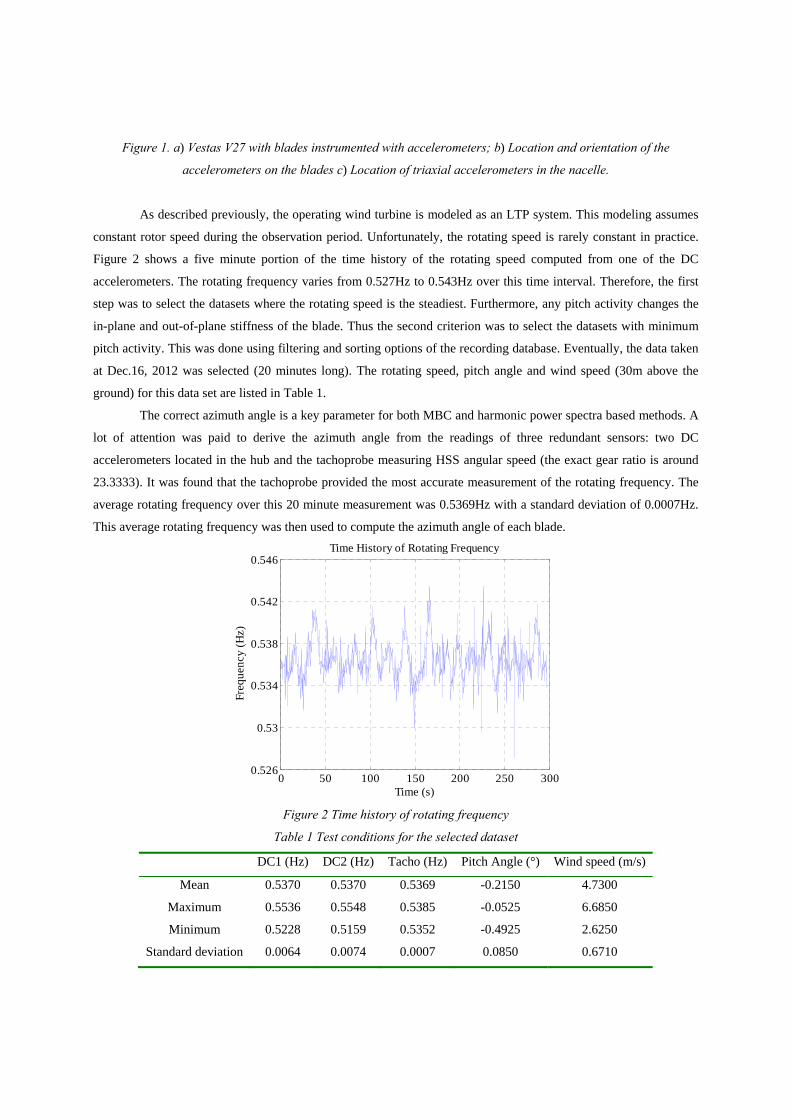
Figure 1. a) Vestas V27 with blades instrumented with accelerometers; b) Location and orientation of the
accelerometers on the blades c) Location of triaxial accelerometers in the nacelle.
As described previously, the operating wind turbine is modeled as an LTP system. This modeling assumes
constant rotor speed during the observation period. Unfortunately, the rotating speed is rarely constant in practice.
Figure 2 shows a five minute portion of the time history of the rotating speed computed from one of the DC
accelerometers. The rotating frequency varies from 0.527Hz to 0.543Hz over this time interval. Therefore, the first
step was to select the datasets where the rotating speed is the steadiest. Furthermore, any pitch activity changes the
in-plane and out-of-plane stiffness of the blade. Thus the second criterion was to select the datasets with minimum
pitch activity. This was done using filtering and sorting options of the recording database. Eventually, the data taken
at Dec.16, 2012 was selected (20 minutes long). The rotating speed, pitch angle and wind speed (30m above the
ground) for this data set are listed in Table 1.
The correct azimuth angle is a key parameter for both MBC and harmonic power spectra based methods. A
lot of attention was paid to derive the azimuth angle from the readings of three redundant sensors: two DC
accelerometers located in the hub and the tachoprobe measuring HSS angular speed (the exact gear ratio is around
23.3333). It was found that the tachoprobe provided the most accurate measurement of the rotating frequency. The
average rotating frequency over this 20 minute measurement was 0.5369Hz with a standard deviation of 0.0007Hz.
This average rotating frequency was then used to compute the azimuth angle of each blade.
Figure 2 Time history of rotating frequency
Table 1 Test conditions for the selected dataset
DC1 (Hz) DC2 (Hz) Tacho (Hz) Pitch Angle (°) Wind speed (m/s)
Mean 0.5370 0.5370 0.5369 -0.2150 4.7300
Maximum 0.5536 0.5548 0.5385 -0.0525 6.6850
Minimum 0.5228 0.5159 0.5352 -0.4925 2.6250
Standard deviation 0.0064 0.0074 0.0007 0.0850 0.6710
0 50 100 150 200 250 3000.526
0.53
0.534
0.538
0.542
0.546Time History of Rotating Frequency
Time (s)
Freq
uenc
y (H
z)

4. Preliminary Analysis
This section describes a preliminary analysis of the measured data, which can be conducted before stepping
into the more complex modeling techniques. For the preliminary analysis, four sensors were selected, see Table 2.
These sensors were located on the trailing edge at the tip, and at 9m from the root of the blade.
Table 2 Acceleration signals selected for analysis
Name (Figure 1b) Description
1f Tip, trailing edge, flapwise direction
3e Tip, trailing edge, edgewise direction
6f 9m from the root, trailing edge, flapwise
8e 9m from the root, trailing edge, edgewise direction
First, the power density spectra (PSD) of the signals was calculated (Δf=1.125·10-2 Hz; block size 89 s; 67%
overlap; Hanning window; 38 averages); the PSD of the tip acceleration signals averaged over 20 minutes of
observation time, are shown in Figure 3. (PSD 1f and 3e [].fig)
Figure 3 PSD of the tip acceleration signals. Blue dash line – rotor fundamental, blue dotted lines – rotor
harmonics; red dashed line – high speed shaft fundamental, red dotted lines – its sidebands.
Analyzing Figure 3, one can observe:
1. The level of the flapwise vibrations is higher than the level of edgewise vibrations;
2. At low frequencies, the response in both flapwise and edgewise directions is heavily dominated by
harmonics. Two families of the harmonics can be identified: the first are the harmonics of the rotor
(shown by the blue vertical lines in Figure 3), the second family is due to the HSS fundamental
frequency at 12.52 Hz modulated by the rotor frequency (the red vertical lines in Figure 3);
0 2 4 6 8 10 12 14 16 1810-6
10-5
10-4
10-3
10-2
10-1
100
101
102
103
104
Frequency, Hz
PS
D (m
/s2 )2 /H
z
Blade A 3eBlade B 3eBlade C 3eBlade A 1fBlade B 1fBlade C 1f

3. The effect of the “fat tails” mentioned in [12] can be clearly seen on the lowest rotor harmonics. The
higher harmonic peaks (starting from the 5th rotor harmonic) become narrower, and eventually have the
appearance of typical harmonic peaks.
4. Flapwise vibrations are less contaminated by the rotor and gearbox harmonics at higher frequencies;
5. The readings of the accelerometers located in the same positions on different blades are not identical,
which is either due to imprecise mounting or different dynamic characteristics of the blades (which is
possible since one of the blade of this particular wind turbine was replaced some years ago). Since the
MBC transformation assumes rotor isotropy and symmetry of the observation system, this could be a
serious obstacle for the application of the MBC-based method. In contrast, the harmonic power
spectrum method does not require these assumptions.
6. Note the double peak at approximately 3.5Hz on the edgewise signal spectra (see the inset): one may
expect a double peak (since the frequencies of the two anti-symmetric modes may slightly differ) but it
is not normal that the higher frequency peak and the lower frequency peak dominate at different blades.
If the rotor was isotropic, the shape of the spectra averaged over many rotor revolutions is expected to
be the same for all three blades. Therefore this observation rather speaks for the rotor anisotropy than
for the imperfection of the sensors mounting.
Since the harmonics are undesirable in further analysis, the time-synchronous averaging (TSA) algorithm
was employed to remove the harmonics. TSA was applied in two runs, first removing the rotor harmonics, and
second – the sidebands of the HSS fundamental frequency. The tacho events are generated from the instantaneous
rotor azimuth ϕ1(t), which is estimated as explained in Section 3. The detailed explanation of the TSA method can
be found in [13]. Due to the “fat tails” phenomena, TSA does not significantly affect the lowest rotor harmonics but
effectively removes the higher harmonics and HSS sidebands.
Along with the PSD, the singular value decomposition (SVD) can shed some light on how many
independent vectors should be used to describe system behavior at different frequencies. The SVD was performed
on the 3x3 cross-spectra matrix computed between the sensors located at the same point on all three blades. Figure 4
shows the three singular values computed for the signal 3e after the harmonics were removed by TSA.

Figure 4 Singular values of the cross-spectra matrices calculated for sensors 3e on all three blades
If focusing on the edgewise vibrations, SVD reveals some expected modal behavior, for example, arrows
#1,2 and #5,6 in Figure 4 denote the two edgewise anti-symmetric modes, #3,#4 are perhaps the edgewise collective
modes, #7,8 are the traces of the two flapwise anti-symmetric modes, which also have an edgewise component.
However, at this point this is just a guess-work; the modal analysis shall reveal the true dynamics of the wind turbine.
The next step will be to apply the MBC transformation to the data according to Eq. (1). The instantaneous
rotor azimuth φ1(t), which participates in Eq. (1) is estimated as explained in Section 3. The geometrical
interpretation of multiblade coordinates can be found in [14]. The spectra of the multiblade coordinates a0, a1 and b1
are shown in Figure 5.
Figure 5 PSD of multiblade coordinates for 3e sensor location.
Analyzing Figure 5, one can observe the following:
0 2 4 6 8 10 12 14 16 18
10-5
10-4
10-3
10-2
10-1
100
101
Frequency, Hz
Sin
gula
r val
ues,
(m/s
2 )2 /Hz
0 2 4 6 8 10 12 14 16 18
10-5
10-4
10-3
10-2
10-1
100
Frequency, Hz
PS
D o
f mul
tibla
de c
oord
inat
es, (
m/s
2 )2 /Hz
a0
a1b1
1 2
34
5 6
7, 8
B A C
E D
F

1. The peak at 1Ω (rotor fundamental) has almost disappeared, while the peak at 3Ω (3rd harmonic, the
so-called blade passing frequency) has increased. This agrees with Bir’s statement that MBC
transformation can be considered as a filter stopping all harmonics except those that are integer
multiples of 3Ω [8].
2. The anti-symmetric coordinates a1 and b1 (green and blue curves respectively) follow each other
closely, in contrast the symmetric (collective) coordinate a0 (red curve) is quite distinct. Thus MBC
effectively separated collective blade behavior from the anti-symmetric.
3. There are two types of behavior of the peaks identified in the blade spectra (Figure 4): some peaks like
peaks #1,2 become two well separated peaks #A,B while the other peaks like #4 keep their location
(peak #C). The first type of peaks is typical for anti-symmetric (or whirling) modes, while the second
type – for collective modes. In blade coordinates, the whirling modes are often very close in
frequencies (e.g. peak pair #1, 2 and pair #5, 6 in Figure 4). In multi-blade coordinates, these peaks are
typically separated: peak pair #1, 2 becomes #A,B and pair #5, 6 becomes #D,E). The distance
between the new peaks in the pairs is about 2Ω.
It is also important to note that the peaks seen on the MBC coordinates (Figure 5) can also be traced in the nacelle
acceleration spectra (Figure 6). This makes it possible to identify many rotor modes using only tower and nacelle
data, was reported in [15].
Figure 6 PSD of the nacelle acceleration signals, side-to-side direction: red – front, green – rear right, blue – rear
left. The letters denoting the peaks are the same as in Figure 5.
5. Modal Analysis of Operational Turbine using Multiblade Coordinate Transformation
The analysis performed so far is purely signal processing, with no modeling introduced and no assumptions
made. In the following sections, we assume that the structure under test is LTP, and will model its dynamics via
modal decomposition.
In this section we perform operational modal analysis (OMA) on the experimentally obtained data pre-
processed by harmonic removal and multiblade coordinate transformation, as detailed in section 4. The new time
histories become the input to OMA. As will be explained later, the main focus is placed on the edgewise motion,
since it has more interesting time-periodic behavior.
2 3 4 5 6 7 8 9 10 11
10-6
10-5
10-4
10-3
10-2
Frequency, Hz
PS
D, (
m/s
2 )2 /Hz
Y FrontY Rear 1Y Rear 2
BA
F

The OMA stochastic subspace identification (SSI) algorithm (Bruel and Kjaer Type 7760) was used for
identification. Twelve channels (3 x (1f, 3e, 6f, 8e, Figure 1b)) were selected for the analysis. The data were
decimated 10 times; thus the new sampling rate is 40.96Hz.
Typically, modal analysis software uses test object geometry in order to visualize measured DOFs and to
animate the modes. In the case of multiblade coordinates such visualization is not physical; however it is found very
useful in order to give mode nomenclature. Figure 8 shows the simple geometry used for the visualization. DOFs
10* denote multiblade coordinate a0, 20* are a1 and 30* are b1. Points *03 correspond to the blade tip, and ones *08
– to the middle of the blade. Z-direction corresponds to flapwise DOFs, and Y – to edgewise direction. If, when
animating the mode, a0 dominates, this is a collective mode. Dominating a1 and b1 indicate anti-symmetric (whirling)
modes. If the phase between a1 and b1 is –900, this is a backward whirling mode; the phase of +900 indicates the
forward whirling. If DOFs *03 and *08 move in-phase, this is a first bending mode, while anti-phase points to the
second bending mode. Identification of higher modes is restricted by the low spatial resolution, especially in the
edgewise direction.
Figure 7 Simple geometry indicating 6 multiblade coordinates
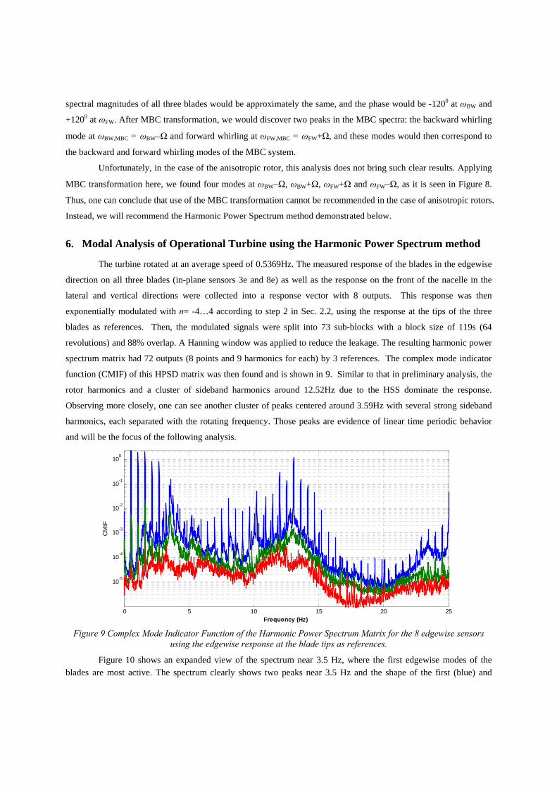
Figure 8 shows the stabilization diagram in the range 2.8-4.4Hz corresponding to peaks #A,B in Figure 6;
the corresponding mode table is shown below. SSI algorithm finds 4 edgewise modes, shown in bold in the table,
the other modes are flapwise dominated or noise modes, which are not considered here. The modes I1BW-1 and
I1FW-1 (abbreviations for in-plane 1st bending, back- or forward whirling respectively) are both originated from the
peak at 3.51Hz on the edgewise signals spectra; the frequencies of these modes are 3.51 Ω respectively. The
modes I1BW-2 and I1FW-2 are originated from the peak at 3.58Hz, and their frequencies are 3.58 Ω. The
presence of the four modes found by OMA-SSI in multiblade coordinate data is an indication of rotor anisotropy;
these modes are not physical, this is an artifact due to the violation of the rotor isotropy assumption.
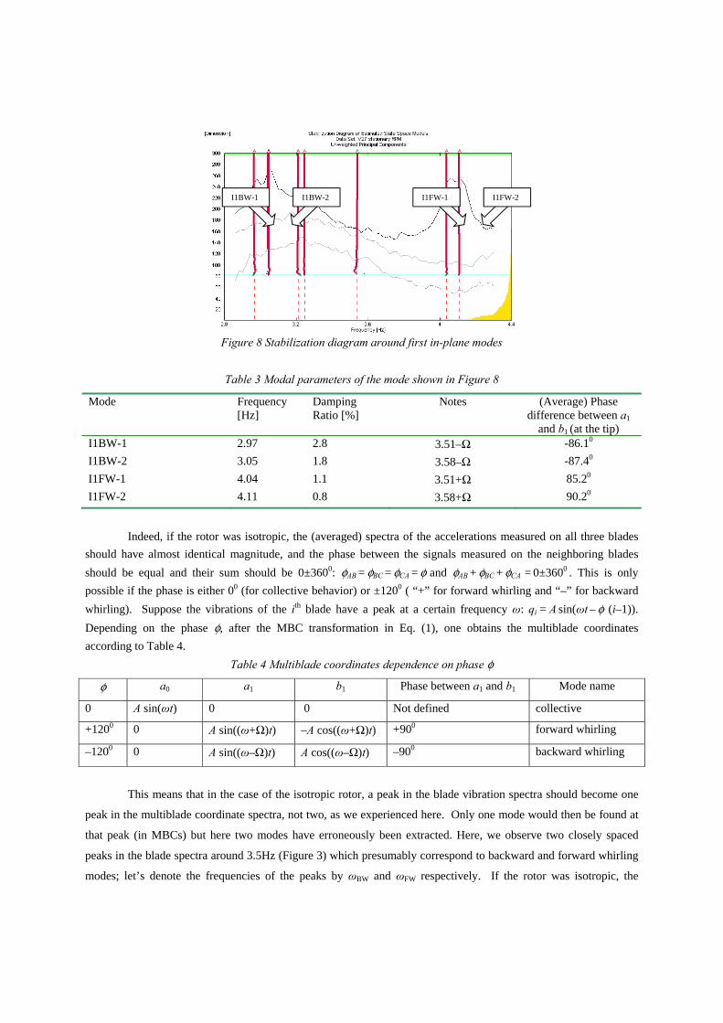
Figure 8 Stabilization diagram around first in-plane modes
Table 3 Modal parameters of the mode shown in Figure 8
Mode Frequency [Hz]
Damping Ratio [%]
Notes (Average) Phase difference between a1
and b1 (at the tip) I1BW-1 2.97 2.8 3.51–Ω -86.10
I1BW-2 3.05 1.8 3.58–Ω -87.40
I1FW-1 4.04 1.1 3.51+Ω 85.20
I1FW-2 4.11 0.8 3.58+Ω 90.20
Indeed, if the rotor was isotropic, the (averaged) spectra of the accelerations measured on all three blades
should have almost identical magnitude, and the phase between the signals measured on the neighboring blades
should be equal and their sum should be 0±3600: φAB = φBC = φCA = φ and φAB + φBC + φCA = 0±3600 . This is only
possible if the phase is either 00 (for collective behavior) or ±1200 ( “+” for forward whirling and “–” for backward
whirling). Suppose the vibrations of the ith blade have a peak at a certain frequency ω: qi = A sin(ωt – φ (i–1)).
Depending on the phase φ, after the MBC transformation in Eq. (1), one obtains the multiblade coordinates
according to Table 4.
Table 4 Multiblade coordinates dependence on phase φ
φ a0 a1 b1 Phase between a1 and b1 Mode name
0 A sin(ωt) 0 0 Not defined collective
+1200 0 A sin((ω+Ω)t) –A cos((ω+Ω)t) +900 forward whirling
–1200 0 A sin((ω–Ω)t) A cos((ω–Ω)t) –900 backward whirling
This means that in the case of the isotropic rotor, a peak in the blade vibration spectra should become one
peak in the multiblade coordinate spectra, not two, as we experienced here. Only one mode would then be found at
that peak (in MBCs) but here two modes have erroneously been extracted. Here, we observe two closely spaced
peaks in the blade spectra around 3.5Hz (Figure 3) which presumably correspond to backward and forward whirling
modes; let’s denote the frequencies of the peaks by ωBW and ωFW respectively. If the rotor was isotropic, the
I1BW-1 I1BW-2 I1FW-1 I1FW-2
spectral magnitudes of all three blades would be approximately the same, and the phase would be -1200 at ωBW and
+1200 at ωFW. After MBC transformation, we would discover two peaks in the MBC spectra: the backward whirling
mode at ωBW,MBC = ωBW–Ω and forward whirling at ωFW,MBC = ωFW+Ω, and these modes would then correspond to
the backward and forward whirling modes of the MBC system.
Unfortunately, in the case of the anisotropic rotor, this analysis does not bring such clear results. Applying
MBC transformation here, we found four modes at ωBW–Ω, ωBW+Ω, ωFW+Ω and ωFW–Ω, as it is seen in Figure 8.
Thus, one can conclude that use of the MBC transformation cannot be recommended in the case of anisotropic rotors.
Instead, we will recommend the Harmonic Power Spectrum method demonstrated below.
6. Modal Analysis of Operational Turbine using the Harmonic Power Spectrum method
The turbine rotated at an average speed of 0.5369Hz. The measured response of the blades in the edgewise
direction on all three blades (in-plane sensors 3e and 8e) as well as the response on the front of the nacelle in the
lateral and vertical directions were collected into a response vector with 8 outputs. This response was then
exponentially modulated with n= -4…4 according to step 2 in Sec. 2.2, using the response at the tips of the three
blades as references. Then, the modulated signals were split into 73 sub-blocks with a block size of 119s (64
revolutions) and 88% overlap. A Hanning window was applied to reduce the leakage. The resulting harmonic power
spectrum matrix had 72 outputs (8 points and 9 harmonics for each) by 3 references. The complex mode indicator
function (CMIF) of this HPSD matrix was then found and is shown in 9. Similar to that in preliminary analysis, the
rotor harmonics and a cluster of sideband harmonics around 12.52Hz due to the HSS dominate the response.
Observing more closely, one can see another cluster of peaks centered around 3.59Hz with several strong sideband
harmonics, each separated with the rotating frequency. Those peaks are evidence of linear time periodic behavior
and will be the focus of the following analysis.
Figure 9 Complex Mode Indicator Function of the Harmonic Power Spectrum Matrix for the 8 edgewise sensors
using the edgewise response at the blade tips as references.
Figure 10 shows an expanded view of the spectrum near 3.5 Hz, where the first edgewise modes of the blades are most active. The spectrum clearly shows two peaks near 3.5 Hz and the shape of the first (blue) and
0 5 10 15 20 25
10-5
10-4
10-3
10-2
10-1
100
Frequency (Hz)
CM
IF

second (green) singular value curves strongly suggests that two modes are present at that peak. Several modulations of the peak are also seen near 3.0, 4.0 and 4.5 Hz. The full harmonic power spectrum matrix was curve fit using a variant of the AMI algorithm [16, 17], focusing only on the peaks near 3.5 Hz. Two modes were identified with natural frequencies 3.5184 and 3.5867 Hz and damping ratios 0.00569 and 0.00355. The mode vectors for each mode are vectors of Fourier coefficients which describe the motion of the mode at the natural frequency, plus motion at nine harmonics of the natural frequency for n = -4…4. This is summarized in Figure 11, which shows the magnitude and phase of the response at several points on the turbine for each harmonic of each of these modes. As the motion is quite a bit more complicated than for an LTI system, some care will be taken to explain the meaning of this result.
Figure 10 Zoom in on Harmonic power spectrum in Fig. 9.
2 2.5 3 3.5 4 4.5 5 5.510-5
10-4
10-3
10-2
10-1
Frequency (Hz)
CM
IF

Figure 11 Identified Fourier coefficients on all the blades plotted against harmonic order a) Harmonic at 3.52Hz b) Harmonic at 3.59Hz
First consider the mode at 3.518 Hz. The mode shape in Figure 11 shows that the motion of the blades is
dominated by motion at the 0th harmonic, or 3.518 Hz. Blade A moves about 180° out of phase with blades B and C.
On the other hand, the tower motion is predominantly at the -1 and 1 harmonics, or 2.982 and 4.055 Hz. This was
evident in Figure 6 which showed the spectrum of the motion of the nacelle. The blades also exhibit some vibration
at these frequencies, although at 4.055 Hz it is about an order of magnitude smaller than the dominant motion and at
2.982 Hz it is smaller still. The higher harmonics (|n|>1) are quite small and so their validity is questionable.
-4 -3 -2 -1 0 1 2 3 410
-3
10-2
10-1
100
101
Mag
nitu
de
a) Harmonics at 3.518 Hz
A-3eB-3eC-3eN10yN10z
-4 -3 -2 -1 0 1 2 3 4-180-135-90-45
04590
135180
Phas
e (o )
Harmonic Order
-4 -3 -2 -1 0 1 2 3 410-4
10-3
10-2
10-1
100
Mag
nitu
de
b) Harmonics at 3.587 Hz
A-3eB-3eC-3eN10yN10z
-4 -3 -2 -1 0 1 2 3 4-180-135
-90-45
04590
135180
Phas
e (o )
Harmonic Order
The mode at 3.587 Hz behaves in a similar manner, with the dominant motion being at the 0th harmonic and
with relatively weak higher harmonics. The motion of the tower is also considerably smaller in this mode. In this
mode blade A is about 45° out of phase with the other two blades and blade B has significantly higher amplitude
than the other blades. It is interesting to note that these two modes do follow the expected trends for the edgewise
modes of an isotropic wind turbine. As illustrated in [6] and [9] and discussed in the previous section, a wind
turbine typically exhibits backward and forward whirling modes, which in the tower reference frame (or in MBCs)
occur at the tower vibration frequencies, or 2.982 and 4.055 Hz in this case. In the blade reference frame these
modes would be closely spaced, and occur approximately equidistant between the two frequencies observed in the
tower. While these modes are typically closely spaced (even repeated for an isotropic turbine, see e.g. [9]) they can
be distinguished by the phase of the motion of the blades as discussed previously. The LTP modes identified for
these two edgewise modes do not seem to follow the expected trends, but fortunately the motion observed is readily
described by a linear time periodic model; the identified time-periodic shapes could be used to predict the motion of
the structure or to validate a model that included the anisotropy of the turbine.
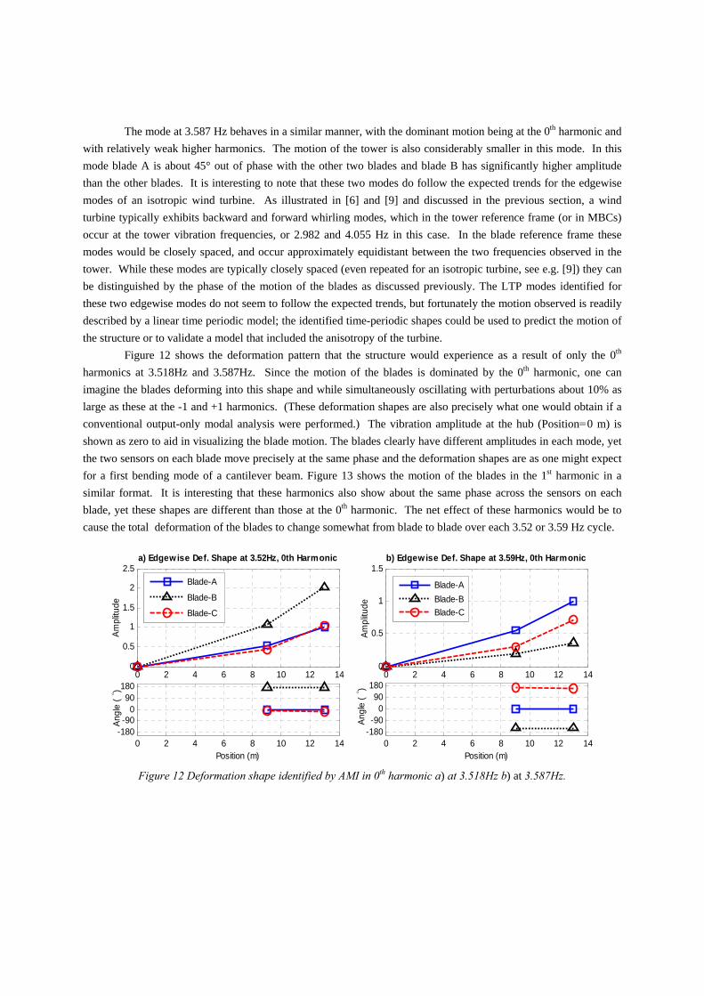
Figure 12 shows the deformation pattern that the structure would experience as a result of only the 0th
harmonics at 3.518Hz and 3.587Hz. Since the motion of the blades is dominated by the 0th harmonic, one can
imagine the blades deforming into this shape and while simultaneously oscillating with perturbations about 10% as
large as these at the -1 and +1 harmonics. (These deformation shapes are also precisely what one would obtain if a
conventional output-only modal analysis were performed.) The vibration amplitude at the hub (Position=0 m) is
shown as zero to aid in visualizing the blade motion. The blades clearly have different amplitudes in each mode, yet
the two sensors on each blade move precisely at the same phase and the deformation shapes are as one might expect
for a first bending mode of a cantilever beam. Figure 13 shows the motion of the blades in the 1st harmonic in a
similar format. It is interesting that these harmonics also show about the same phase across the sensors on each
blade, yet these shapes are different than those at the 0th harmonic. The net effect of these harmonics would be to
cause the total deformation of the blades to change somewhat from blade to blade over each 3.52 or 3.59 Hz cycle.
Figure 12 Deformation shape identified by AMI in 0th harmonic a) at 3.518Hz b) at 3.587Hz.
0 2 4 6 8 10 12 140
0.5
1
1.5
2
2.5
Ampl
itude
a) Edgewise Def. Shape at 3.52Hz, 0th Harmonic
0 2 4 6 8 10 12 14-180-90
090
180
Angl
e (
° )
Position (m)
Blade-A
Blade-B
Blade-C
0 2 4 6 8 10 12 140
0.5
1
1.5
Ampl
itude
b) Edgewise Def. Shape at 3.59Hz, 0th Harmonic
0 2 4 6 8 10 12 14-180-90
090
180
Angl
e (
° )
Position (m)
Blade-ABlade-BBlade-C

Figure 13 Deformation shape identified by AMI in 1st harmonic for modes centered at a) at 3.518Hz b) at 3.587Hz.
7. Conclusion
An operating wind turbine has to be modeled as an LTP system to correctly characterize its time periodic
behavior. In this work, two methods suitable for LTP systems, namely, the multiblade coordinate transformation and
the harmonic power spectrum, were employed to identify the modes of an operating wind turbine. The vibration data
were obtained from an operating Vestas V27 wind turbine instrumented with accelerometers on the blades and the
nacelle.
From the accelerometer readings, it was observed that the wind turbine rotor is anisotropic; therefore the
MBC transformation will fail to convert the LTP system into an LTI system. It was shown that application of the
MBC transformation lead to erroneous results. In contrast, the harmonic power spectrum does not require the rotor
to be isotropic. The method was successfully applied; for demonstration purposes, and two edgewise (in-plane)
bending modes were identified and analyzed in detail. In this particular case, the experimental data revealed that the
magnitude of the sideband harmonics in the blade reference frame was an order of magnitude lower than the central
frequency component. If these sidebands were negligible then one could use straightforward operational modal
analysis on the data. However, then one is faced with a dilemma because the same modes appear at different
frequencies in the tower measurements. In any event, the harmonic spectrum method allows on to easily identify the
harmonic content in each mode and to robustly determine the number of modes present in the data.
Comparing the two methods in application to experimental modal analysis of operating wind turbine, the
harmonic power spectrum method is strongly recommended for most cases. Firstly, since the rotor isotropy is not
initially known, using of MBC transformation may result in an erroneous modal identification. Secondly, the MBC
method requires instrumentation of all three blades and, besides this, a precise symmetric mounting of
accelerometers on the blades. If the sensors on one blade should fail then the method cannot be used. The harmonic
power spectrum method does not require this, which makes it is much more practical in a real life situation. The
harmonic power spectrum directly identifies the natural frequencies, damping ratios and the periodically time-
varying modes that describe the motion of the blades in the rotating frame and the motion of the tower in the fixed
frame. These modal parameters can be compared with the analytically derived modes of the turbine, obtained
0 2 4 6 8 10 12 140
0.05
0.1
0.15
0.2
Ampl
itude
Edgewise Def. Shape at 3.52Hz, 1st Harmonic
Blade-ABlade-BBlade-C
0 2 4 6 8 10 12 14-180-90
090
180
Ang
le (
° )
Position (m)
0 2 4 6 8 10 12 140
0.05
0.1
Ampl
itude
Edgewise Def. Shape at 3.59Hz, 1st Harmonic
Blade-ABlade-BBlade-C
0 2 4 6 8 10 12 14-180-90
090
180
Ang
le (
° )
Position (m)

through a Floquet analysis, to validate an anisotropic model for the turbine. The methods will be further compared
and these ideas will be further developed in the next stage of the work.
References:
[1] R.P.Coleman, "Theory of self-excited mechanical oscillations of hinged rotor blades," available from <ntrs.nasa.gov>, Langley Research Center1943.
[2] M. H. Hansen, "Improved modal dynamics of wind turbines to avoid stall-induced vibrations," Wind Energy, vol. 6, pp. 179-195, 2003.
[3] D. Tcherniak and G. C. Larsen, "Applications of OMA to an operating wind turbine: now including vibration data from the blades," presented at the 5th International Operational Modal Analysis Conference, Guimarães - Portugal, 2013.
[4] D. Tcherniak, S. Chauhan, M. Rossetti, I. Font, J. Basurko, and O. Salgado, "Output-only Modal Analysis on Operating Wind Turbines: Application to Simulated Data," presented at the European Wind Energy Conference, Warsaw, Poland, 2010.
[5] N. M. Wereley, "Analysis and Control of Linear Periodically Time Varying Systems," PhD, Department of Aeronautics and Astronautics, Massachusetts Institute of Technology, Cambridge, 1991.
[6] M. S. Allen, M. W. Sracic, S. Chauhan, and M. H. Hansen, "Output-Only Modal Analysis of Linear Time Periodic Systems with Application to Wind Turbine Simulation Data," Mechanical Systems and Signal Processing, vol. 25, pp. 1174-1191, 2011.
[7] S. Yang and M. S. Allen, "Output-Only Modal Analysis Using Continuous-Scan Laser Doppler Vibrometry and Application to a 20kW Wind Turbine," Mechanical Systems and Signal Processing, vol. 31, August 2012 2011.
[8] G. Bir, "Multiblade Coordinate Transformation and Its Application to Wind Turbine Analysis," presented at the 2008 ASME Wind Energy Symposium, Reno, Nevada, 2008.
[9] P. F. Skjoldan and M. H. Hansen, "On the similarity of the Coleman and Lyapunov-Floquet transformations for modal analysis of bladed rotor structures," Journal of Sound and Vibration, vol. 327, pp. 424-439, 2009.
[10] S. Yang and M. S. Allen, "A Lifting Algorithm for Output-only Continuous Scan Laser Doppler Vibrometry," presented at the AIAA, Hawaii, 2012.
[11] C.-T. Chen, Linear system theory and design, 3rd edtion ed.: Oxford University Press, Inc, 1999. [12] D. Tcherniak, S. Chauhan, and M. H. Hansen, "Applicability limits of Operational Modal Analysis to
Operational wind turbines," presented at the 28th International Modal Analysis Conference (IMAC XXVIII), Jacksonville, Florida, 2010.
[13] T.Jacob, D.Tcherniak, and R.Castiglione, "Harmonic Removal as a Pre-processing Step for Operational Modal Analysis: Application to Operating Gearbox Data," presented at the VDI-Fachtagung Schwingungen von Windenergieanlagen 2014.
[14] M. H. Hansen, "Aeroelastic stability analysis of wind turbines using an eigenvalue approach," Wind Energy, vol. 7, pp. 133-143, 2004.
[15] D. Tcherniak, J. Basurko, O. Salgado, I. Urresti, S. Chauhan, C.E.Carcangui, and M. Rossetti, "Application of OMA to Operational Wind Turbine," presented at the International Operational Modal Analysis Conference, Istanbul, Turkey, 2011.
[16] M. S. Allen, "Global and Multi-Input-Multi-Output (MIMO) Extensions of the Algorithm of Mode Isolation (AMI)," Doctorate, George W. Woodruff School of Mechanical Engineering, Georgia Institute of Technology, Atlanta, Georgia, 2005.
[17] M. S. Allen and J. H. Ginsberg, "A Global, Single-Input-Multi-Output (SIMO) Implementation of The Algorithm of Mode Isolation and Applications to Analytical and Experimental Data," Mechanical Systems and Signal Processing, vol. 20, pp. 1090–1111, 2006.