mixed logit with repeated choices: households - university of

1

Mixed Logit with Repeated Choices:

Households’ Choices of Appliance Efficiency Level

by

David Revelt and Kenneth Train

Department of Economics

University of California, Berkeley

July 1997

Forthcoming, Review of Economics and Statistics

Abstract: Mixed logit models, also called random-parameters or error-components logit, are a

generalization of standard logit that do not exhibit the restrictive "independence from irrelevant

alternatives" property and explicitly account for correlations in unobserved utility over repeated

choices by each customer. Mixed logits are estimated for households' choices of appliances under

utility-sponsored programs that offer rebates or loans on high-efficiency appliances.

JEL Codes: C15, C23, C25, D12, L68, L94, Q40

2

Mixed Logit with Repeated Choices:

Households’ Choices of Appliance Efficiency Level

1. Introduction

Mixed logit (also called random-parameters logit) generalizes standard logit by allowing the

parameter associated with each observed variable (e.g., its coefficient) to vary randomly across

customers. The moments of the distribution of customer-specific parameters are estimated. Variance

in the unobserved customer-specific parameters induces correlation over alternatives in the stochastic

portion of utility. As a result, mixed logit does not exhibit the restrictive forecasting patterns of

standard logit (i.e., does not exhibit independence from irrelevant alternatives.) Mixed logit also

allows efficient estimation when there are repeated choices by the same customers, as occurs in our

application.

Mixed logits have taken different forms in different applications; their commonality arises in the

integration of the logit formula over the distribution of unobserved random parameters. The early

applications (Boyd and Mellman, 1980, and Cardell and Dunbar, 1980) were restricted to situations

in which explanatory variables do not vary over customers, such that the integration, which is

computationally intensive, is required for only one "customer" using aggregate share data rather than

for each customer in a sample. Advances in computer speed and in our understanding of simulation

methods for approximating integrals have allowed estimation of models with explanatory variables

varying over customers. Ben-Akiva et al (1993), Ben-Akiva and Bolduc (1996), Bhat (1996), and

Brownstone and Train (1996) apply a mixed logit specification like that given below but without

repeated choices. Other empirical studies (Berkovec and Stern, 1991; Bolduc et al, 1993; and Train

et al, 1987) have specified choice probabilities that integrate a logit function over unobserved terms,

but with these terms representing something other than random parameters of observed attributes.

In all cases except Ben-Akiva et al (1993) and Train et al (1987), the integration is performed through

simulation, similar to that described below. These two exceptions used quadrature, which was feasible

in their cases because only one- or two-dimensional integration was required in their specifications.

Lnit(�n) e�n1xnit

�j

e�n1xnjt

3

Terminology for these models varies. "Random-coefficients logit" or “random-parameters logit” has

been used for obvious reasons (Ben-Akiva and Lerman, 1985; Bhat, 1996; Train, 1996). The term

“error-components logit” is useful since it emphasizes the fact that the unobserved portion of utility

consists of several components and that these components can be specified to provide realistic

substitution patterns rather than to represent random parameters per se (Brownstone and Train,

1996). “Mixed logit" reflects the fact that the choice probability is a mixture of logits with a specified

mixing distribution (Brownstone and Train, 1996; McFadden and Train, 1997; Train 1997.) This term

encompasses any interpretation that is consistent with the functional form. We use “mixed logit” in

the current paper because of this generality, even though our specification is motivated through a

random-parameters concept. Ben-Akiva and Bolduc (1996) use the term "probit with a logit kernel"

to describe models where the customer-specific parameters are normally distributed. This term is

instructive since it points out that the distinction between pure probits (in which utility is normally

distributed) and mixed logits with normally distributed parameters is conceptually minor.

2. Specification

A person faces a choice among the alternatives in set J in each of T time periods or choice situations.

The number of choice situations can vary over people, and the choice set can vary over people and

choice situations. The utility that person n obtains from alternative j in choice situation t is U =njt

� 1x + J where x is a vector of observed variables, coefficient vector � is unobserved for eachn njt njt njt n

n and varies in the population with density f(� |�*) where �* are the (true) parameters of thisn

distribution, and J is an unobserved random term that is distributed iid extreme value, independentnjt

of � and x . Conditional on � , the probability that person n chooses alternative i in period t isn njt n

standard logit:

(1)

The unconditional probability is the integral of the conditional probability over all possible values of

4

� , which depends on the parameters of the distribution of � :n n

Q (�*) = , L (� ) f(� |�*) d � . nit nit n n n

For maximum likelihood estimation we need the probability of each sampled person's sequence of

observed choices. Let i(n,t) denote the alternative that person n chose in period t. Conditional on � ,n

the probability of person n's observed sequence of choices is the product of standard logits:1

S (� ) = - L (� ).n n t ni(n,t)t n

The unconditional probability for the sequence of choices is:

(2) P (�*) = , S (� ) f(� |�*) d� .n n n n n

Note that there are two concepts of parameters in this description. The coefficient vector � is then

parameters associated with person n, representing that person's tastes. These tastes vary over people;

the density of this distribution has parameters �* representing, for example, the mean and covariance

of � . The goal is to estimate �*, that is, the population parameters that describe the distribution ofn

individual parameters.

The log-likelihood function is LL(�)=� lnP (�). Exact maximum likelihood estimation is not possiblen n

since the integral in (2) cannot be calculated analytically. Instead, we approximate the probability

through simulation and maximize the simulated log-likelihood function. In particular, P (�) isn

approximated by a summation over randomly chosen values of � . For a given value of the parametersn

�, a value of � is drawn from its distribution. Using this draw of � , S (� ) -- the product of standardn n n n

logits -- is calculated. This process is repeated for many draws, and the average of the resulting

S (� )'s is taken as the approximate choice probability:n n

SSn(�) �0lnSPn(�)

0�

1SPn(�)

1R

�rSn(�

r|�n ) �

t�j(dnjtL r|�

njt )0�

r|�n 1xnjt

0�

5

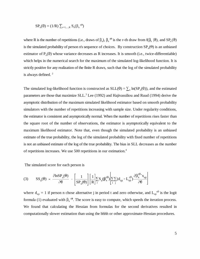
SP (�) = (1/R) � S (� )n r=1,...,R n n r|�

where R is the number of repetitions (i.e., draws of � ), � is the r-th draw from f(� |�), and SP (�)n n n n r|�

is the simulated probability of person n's sequence of choices. By construction SP (�) is an unbiasedn

estimator of P (�) whose variance decreases as R increases. It is smooth (i.e., twice-differentiable)n

which helps in the numerical search for the maximum of the simulated log-likelihood function. It is

strictly positive for any realization of the finite R draws, such that the log of the simulated probability

is always defined. 2

The simulated log-likelihood function is constructed as SLL(�) = � ln(SP (�)), and the estimatedn n

parameters are those that maximize SLL. Lee (1992) and Hajivassiliou and Ruud (1994) derive the3

asymptotic distribution of the maximum simulated likelihood estimator based on smooth probability

simulators with the number of repetitions increasing with sample size. Under regularity conditions,

the estimator is consistent and asymptotically normal. When the number of repetitions rises faster than

the square root of the number of observations, the estimator is asymptotically equivalent to the

maximum likelihood estimator. Note that, even though the simulated probability is an unbiased

estimate of the true probability, the log of the simulated probability with fixed number of repetitions

is not an unbiased estimate of the log of the true probability. The bias in SLL decreases as the number

of repetitions increases. We use 500 repetitions in our estimation. 4

The simulated score for each person is

(3)

where d = 1 if person n chose alternative j in period t and zero otherwise, and L is the logitnjt njtr|�

formula (1) evaluated with � . The score is easy to compute, which speeds the iteration process.n r|�

We found that calculating the Hessian from formulas for the second derivatives resulted in

computationally slower estimation than using the bhhh or other approximate-Hessian procedures.

6

In general, the coefficient vector can be expressed as � = b + � , where b is the population mean andn n

� is the stochastic deviation which represents the person's tastes relative to the average tastes in then

population. Then U = b1x + � 1x +J . In contrast to standard logit, the stochastic portion ofnjt njt n njt njt

utility, � 1x +J , is in general correlated over alternatives and time due to the common influencen njt njt

of � . Mixed logit does not exhibit the independence from irrelevant alternatives property of standardn

logit, and very general patterns of correlation over alternatives and time (and hence very general

substitution patterns) can be obtained through appropriate specification of variables and parameters.

In fact, McFadden and Train (1997) show that any random-utility model can be approximated to any

desired degree of accuracy with a mixed logit through appropriate choice of explanatory variables

and distributions for the random parameters. In the application below, we estimate models with5

normal and log-normal distributions for elements of � ; other distributions are of course possible. n

3. Application

Demand side management (DSM) programs by electric utilities have relied heavily on rebates as a

mechanism for promoting energy efficiency. As the electricity industry moves toward greater

competition, the feasibility of rebates is questionable. Low-interest loan programs are being

considered as alternatives. Potentially, loans can provide an incentive for efficiency, and so serve the

goals of DSM, and yet generate profits as long as the interest rates on the loans are above the firm's

cost of capital.

Using data from Southern California Edison (SCE), we estimate the impact of rebates and loans on

residential customers' choice of efficiency level for refrigerators. Since loans have not been offered

by SCE in the past, and there has been little variation in rebate levels, data on actual purchases by

SCE customers do not provide the information needed to estimate choice models with loan terms and

rebate levels as explanatory variables. Stated-preference data were collected to estimate such models.

In particular, a sample of SCE's residential customers were presented in a survey situation with a

series of choice experiments. In each experiment, two or three refrigerators with different efficiency

levels were described, with a rebate, loan, or no incentive offered on the high efficiency units. The

7

customer was asked which appliance he/she would choose. These stated-preference data were

supplemented, insofar as possible, with information on the efficiency level of the refrigerator that the

customer actually purchased, for customers who had bought a refrigerator within the last three years.

Mixed logits are estimated on the stated-preference data; the models are then adjusted, or

"calibrated," to reflect the limited revealed-preference data. The calibrated models are then used to

forecast the impact of various loan programs.

In the stated-preference choice experiments, each sampled customer was offered a series of binary

choices, followed by a series of trinary choices. For the binary choices, the purchase price and

operating cost of a standard efficiency and a high efficiency refrigerator were described and the

customer was asked which he/she would choose. The high efficiency unit was offered either without

any incentive, with a rebate, or with a financing package with specified interest rate, amount

borrowed, repayment period, and monthly payment. Trinary choices were then offered to the

customer. In these experiments, the customer was offered three high efficiency units, one with no

incentive, one with a rebate, and one with financing. The purchase price and operating cost of the

units differed, such that the unit with no incentive was not dominated. In total, responses to 6081

choice experiments were obtained from 401 surveyed customers, with each customer providing

responses to 12 binary choice experiments and up to four trinary experiments. The 6081 experiments

consists of the following types: 1604 pair a standard unit with a high efficiency unit that has no

incentive, 1626 pair a standard unit with a high efficiency unit on which a rebate is available, 1602

pair a standard unit with a high efficiency unit on which a loan is offered, and 1249 include three high

efficiency units with no incentive, a rebate, and a loan. 6

The choice experiments were designed to provide plausible attributes, orthogonal over experiments,

and with no experiment containing a dominated alternative. The variables that enter the models below

are: (a) Price of the refrigerator, net of any rebate, in hundreds of dollars. For a standard-efficiency

unit and high efficiency units without a rebate, this variable is the price of the unit. For high efficiency

units with a rebate, it is the price of the unit minus the rebate. (b) Savings, in hundreds of dollars.7

This variable is zero for the standard unit and, for the high efficiency units, is the annual dollar

0�r|�n 1xnjt

0bk

xk,njt

0�r|�n 1xnjt

0Wk

µrkxk,njt ,

8

reduction in operating cost that the unit provides relative to the standard unit. (That is, savings in any

experiment is the operating cost of the standard unit minus the operating cost of the high efficiency

unit.) (c) Amount borrowed, in hundreds of dollars. This variable is zero for standard units and for

high efficiency units for which no loan is offered. For high efficiency units on which a loan is offered,

this variable is the maximum dollar amount that customer is allowed to borrow. The percent of the

purchase price that the customer is able to borrow varies over experiments. (d) Interest rate, in digits

(i.e., 4% interest is entered as 0.04). This variable is zero for standard units and for high efficiency

units for which no loan is offered. For high efficiency units with a loan being offered, the variable is

the interest rate that is offered for the loan. The interest rate varies over experiments. (e) Efficiency

dummy. This variable takes the value of zero for standard units and one for high efficiency units. (f)

Rebate dummy, taking the value of one for high efficiency units on which a rebate is provided, and

zero otherwise. (g) Finance dummy, taking the value of one for high efficiency units for which a loan

is provided, and zero otherwise. The means of these variables over the choice experiments are given

in Table 1. Details of the survey design and variables are provided in SCE(1994).

Model estimation

We specify the price coefficient to be fixed while allowing the other coefficients vary. The

willingness-to-pay for each attribute (which is the ratio of the attribute's coefficient to the price

coefficient) is thereby distributed in the same way as the attribute's coefficient, which is convenient

for interpretation of the model. 8

We first specify all the non-price coefficients to be independently normally distributed. The coefficient

vector is expressed as � =b+Wµ where W is a diagonal matrix whose elements are standardn n

deviations (with the top-left element being zero, for the price coefficient) and µ is a vector ofn

independent standard normal deviates. For simulation, draws of µ are obtained from a pseudo-n

random number generator, and the corresponding draws of � are calculated for any given values ofn

the means b and standard deviations W. With this specification, the derivatives that enter the score

(3) are and where the subscript k denotes the k-th element.

9

Subsequent models allow correlation among the coefficients and specify log-normal distributions for

some of the coefficients.

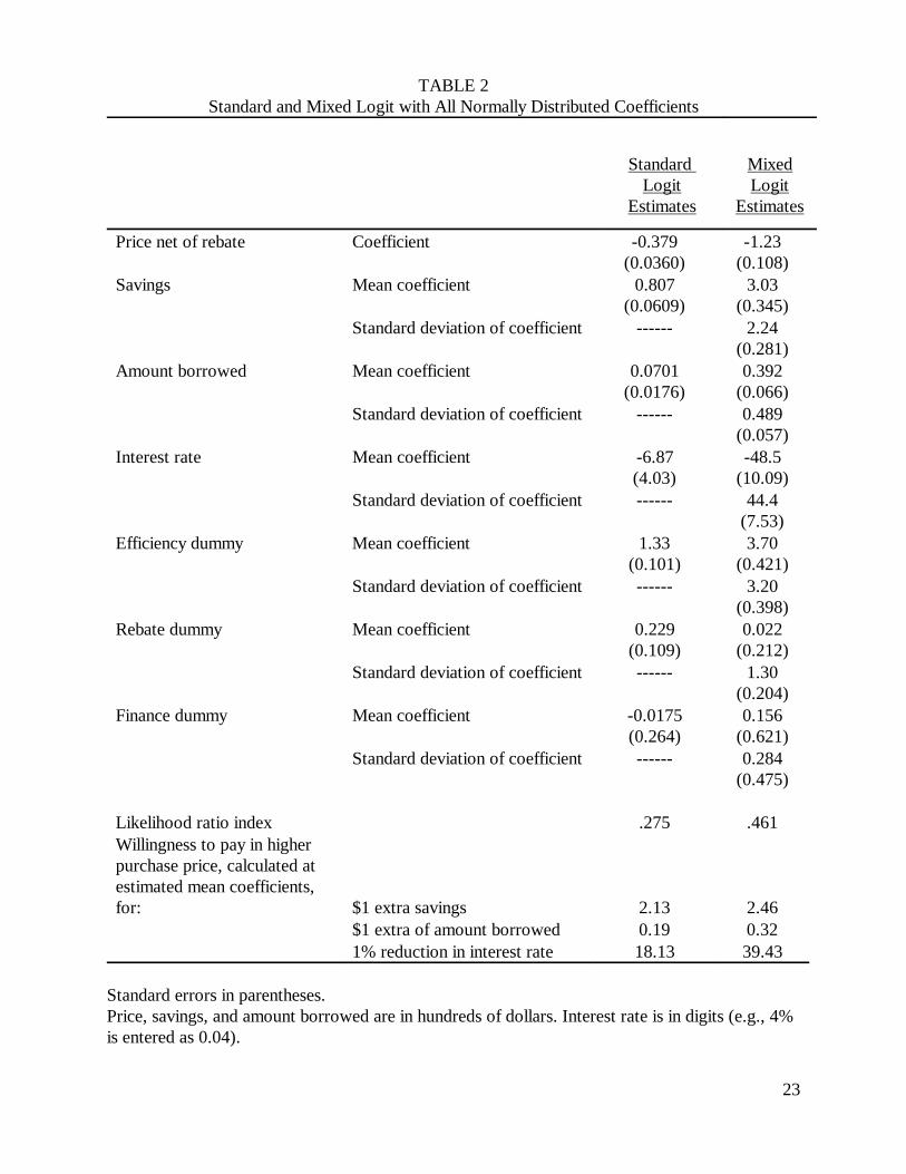
Table 2 provides the estimation results for this model, along with the results for a standard logit

model. The mean coefficients in the mixed logit are consistently larger than the fixed coefficients in

the standard logit model. This result reflects the fact that the mixed logit decomposes the unobserved

portion of utility and normalizes parameters on the basis of part of the unobserved portion. Suppose

true utility is given by the mixed logit: U = b1x + µ 1Wx +J . The parameters b are normalizednjt njt n njt njt

such that J has the appropriate variance for an extreme value error. The standard logit model treatsnjt

utility as U = b1x + ! with b normalized such that ! has the variance of an extreme valuenjt njt njt njt

deviate. The extreme value term in the standard logit model incorporates any variance in the

parameters. In the mixed logit, the variance in parameters is treated explicitly as a separate

component of the error (µ1Wx ) such that the remaining error (J ) is "net" of this variance. Sincen njt njt

the variance in the error term in the standard logit is greater than the variance in the extreme value

component of the error term in the mixed logit, the normalization makes the parameters in the

standard logit model smaller in magnitude than those in the mixed logit. The fact that the parameters

rise by a factor of three or more implies that the random parameters constitute a very large share of

the variance in unobserved utility.

In the mixed logit, the estimated standard deviations of coefficients are highly significant, indicating

that parameters do indeed vary in the population. Also, the likelihood ratio index rises substantially9

from allowing the parameters to vary, indicating that the explanatory power of the mixed logit is

considerably greater than with standard logit. The magnitudes of the estimated standard deviations10

are reasonable relative to the estimated means. For example, the distribution of the savings coefficient

has an estimated mean of 3.03 and an estimated standard deviation of 2.24. Given the estimated price

coefficient, the model implies that the willingness to pay for one dollar of annual savings, on the

margin, is normally distributed in the population with mean of $2.46 and standard deviation of $1.81

-- which is a fairly substantial variation in willingness to pay. The standard logit model implies a

willingness to pay of $2.12. If customers consider refrigerators to have a ten year life, and expect no

10

real growth in energy prices, a willingness to pay of $2.12 implies a discount rate of 46%, and $2.46

implies a discount rate of 39%. These implicit discount rates, while high relative to interest rates,11

are consistent with previous findings on residential customers' choice of refrigerator efficiency levels

(e.g., Cole and Fuller, 1980; McRae, 1980; Meier and Whittier, 1983.)

The mixed logit implies that about 9% of the population place a negative coefficient on savings. This

implication could reflect reality or could be an artifact of the assumption of normally distributed

coefficients. It is possible that some customers are highly skeptical of energy conservation claims and

become more mistrustful the greater the claim of savings is. In this case, negative coefficients for

savings reflect the mistrust of these customers and are an accurate representation of reality. On the

other hand, the assumption of a normal distribution implies that some share of the population has

negative coefficients for savings, whether or not this is true. This issue is addressed below with a

model that specifies a log-normal distribution for the coefficients of savings and other variables.

The parameters associated with amount borrowed imply that the mean willingness to pay for being

able to borrow an extra dollar is $0.32 and the standard deviation is $0.40. Interest rates are denoted

in digits (e.g., an interest rate of 9% is denoted as 0.09). The mean willingness to pay for a 1%

reduction in interest rate is therefore $39 with a standard deviation of $36. For both the interest rate

and amount borrowed, the variation in coefficients is fairly substantial, implying that different people

respond quite differently to loan terms.

An efficiency dummy enters the utility of high-efficiency refrigerators, whether or not an incentive

is offered on the unit. Its mean coefficient indicates that, on average, customers choose the high

efficiency unit in the choice experiments more readily than can be explained by the price, savings, and

other financial matters. The standard deviation indicates that 88% of the population have a "high

efficiency preference". This "preference" is largely an artifact of the experiments, where customers

perhaps feel that the interviewer wants them to say they would purchase the high efficiency unit, or

would think well of them if they did. When the model is calibrated against revealed-choice data

below, the mean drops considerably. However, it is still significantly different from zero, indicating

11

that there is some preference for high efficiency units, independent of price and savings, even in

customers' actual choices. This preference might indicate that customers think that high efficiency is

correlated with higher quality, greater durability, less noise, or other desirable attributes.

Rebates can be viewed by customers in a variety of ways independent of the reduction in price that

they provide. Customers seem to be skeptical of information from their energy utility, including

information about the supposed savings that high-efficiency appliances provide (Constantzo, et al.,

1986; Bruner and Vivian, 1979; Craig and McCann, 1978). For some customers, the offer of a rebate

lends credibility to the savings claim: these customers interpret the rebate as evidence that the utility

is willing to "put its money where its mouth is" (Train, 1988). For these customers, the rebate dummy

has a positive coefficient. Other customers might see the rebate as the opposite kind of signal, namely,

as a sign that the appliances are too poor to sell on their own merit. These customers have a negative

coefficient for the rebate dummy. Table 2 indicates that the mean coefficient for the rebate dummy

is slightly positive but not significantly different from zero, while the standard deviation is fairly large

and highly significant. These results indicate that there is a wide variety of views that customers hold

about rebates, with about as many seeing the rebates as a negative signal as see it as a positive signal.

Note that the standard logit model masks this reality: its slightly positive coefficient for the rebate

dummy would be interpreted as indicating that customers in general view rebates as a slightly positive

signal, while in reality, many customers view rebates as a negative signal and many view it as a strong

positive signal. It is simply that the customers who take the rebate as a negative signal nearly balance

the customers who take it as a positive signal, such that the mean effect is only slightly positive.

The coefficient of the financing dummy obtains an insignificant mean and standard deviation: the

hypothesis that customers examine loans only on the basis of their financial terms cannot be rejected.

The difference in how customers respond to loans versus rebates is plausible. Rebates are a "give-

away;" customers naturally wonder about the motivation for the give-away and tend to read a signal

into it even if there is none. Loans are not a give-away; the customer realizes that the lender makes

money from the loans. The customer need not read a signal into the offer of loans, since the

motivation for the offer is clear.

12

Several variations on this basic model were estimated to explore particular issues. These models are

described below.

The estimates in Table 2 indicate that parameters vary greatly in the population. However, the

specification does not include observed characteristics of the customer. Variations in parameters that

are related to observed characteristics can be captured in standard logit models through interaction

of customer characteristics with attributes of the alternatives. The question arises, therefore: to what

extent can the variation in parameters that is evidenced in Table 2 be captured through the inclusion

of customer characteristics? Table 3 presents a model that includes the income and the education level

of the customer interacted with the price of the refrigerator. This specification follows Atherton and

Train (1995), which was obtained after extensive testing with the demographic variables that were

available from the survey. In this model, willingness to pay for each attribute varies with income and

education, since the price variable is interacted with these factors. The standard deviations are still

large and significant, which indicates that willingness to pay varies more than is captured by the

income and education of customers. There are probably other potentially observable characteristics

that relate to willingness to pay; the fact that only education and income enter this model reflects the

limited nature of the socio-demographic information that was available from the survey.

The model in Table 2 specifies the coefficients to be independently distributed while, in reality, one

would generally expect correlation. For example, customers who are especially concerned about

savings in their monthly energy bill might also be concerned about interest rates, particularly since

the loan payments will appear on their monthly energy bill. To investigate these possibilities, we

specify � ~N(b,6) for general 6. The coefficient vector is expressed � =b+Lµ where L is a lower-n n n

triangular Choleski factor of 6, such that LL1=6. We estimate b and L, and calculate standard errors

for elements of 6 with the derivative rule . The ratios of estimated means are very similar to those12

in Table 2, with similar levels of significance; their magnitudes are somewhat higher, reflecting the

fact that allowing for covariances captures more variance in the unobserved portion of utility, such

that J has less variance and the normalization raises the parameters. The estimates of b and L are not

reported, since the estimates of b have the same interpretation as for Table 2 and the estimates of L

13

have no meaning in themselves. Table 4 gives the estimated covariance matrix, t-statistics for the

estimated covariance matrix, and point estimates for the correlation matrix. Five covariances have t-

statistics over 1.6. (i) The savings coefficient is negatively correlated with the coefficient of the

efficiency dummy. This estimate implies that customers who value savings highly tend not to be

motivated by the label of high-efficiency independent of savings. (ii) The savings coefficient is

negatively correlated with the rebate dummy coefficient, implying that customers who value savings

highly tend not to be motivated by rebates beyond the reduction in price that the rebates provide. (iii-

iv) The efficiency dummy coefficient is positively correlated with the coefficient of amount borrowed

and negatively with the finance dummy coefficient. Customers who like high-efficiency per se

(independent of savings) like being able to borrow a lot and are not motivated by the offer of a loan

independent of its terms. (v) The coefficients of the rebate and finance dummies are positively

correlated: customers who are motivated by rebates beyond the reduction in price that the rebates

provide are also motivated by the offer of a loan beyond the terms of the loan.

The normal distribution allows coefficients of both signs. For some variables, such as savings, it is

reasonable to expect that all customers have the same sign for their coefficients. We estimate a model

with log-normal distributions for the coefficients of savings, amount borrowed, and interest rates. The

coefficients for the efficiency, rebate and finance dummies are kept as normals, since these coefficients

can logically take either sign for a given individual. Let k denote an element of � that has a log-n

normal distribution. This coefficient is expressed � = exp(b + s µ ) where µ is an independentnk k k nk nk

standard normal deviate. The parameters b and s , which represent the mean and standard deviationk k

of log(� ), are estimated. The median, mean, and standard deviation of � are: exp(b ),nk nk k

exp(b +(s /2)), and mean*�[exp(s )-1], respectively. Savings and amount borrowed enter directly,k k k2 2

such that all customers' coefficients are positive, and the negative of interest rates is entered such that

all customers' coefficients of interest rate are negative. Table 5 gives the estimation results. The

results are similar qualitatively to those obtained with all normal distributions. Each of the three log-

normal distributions has median and mean that bracket the mean that is obtained with a normal

distribution. For example, from Table 5, the estimated median willingness-to-pay for savings is $1.81

with an estimated mean of $3.23, while the mean/median with a normal distribution is $2.46. It is13

14

interesting to note that the log-likelihood value is lower for the model with log-normal distributions

than the comparable model (Table 2) with all normally distributed coefficients. A possible reason is

discussed in footnote fourteen. For calibration and simulation, we utilize both models.

Calibration to revealed-preference data

Once estimated, the models are calibrated to the limited revealed-preference data that were available.

Each surveyed customer was asked whether he/she had purchased a refrigerator during the last three

years. Those who responded in the positive were asked to locate the serial number or other

identifying information for the unit that they purchased. With this information, we determined, using

product specification sheets, the efficiency level of the refrigerator. Program files were then used to

determine which of the customers who had purchased a high efficiency refrigerator had received a

rebate. In combination, this information identified whether the customer had chosen standard

efficiency, high efficiency without a rebate, or high efficiency with a rebate. The information was

obtained for 163 of the 401 surveyed customers. Of course, since financing had not been offered by

SCE's programs, a high efficiency unit with utility financing was not available.

Actual choices are expected to differ from stated choices for two primary reasons. First, customers

might have a tendency to say that they would purchase a high efficiency refrigerator more readily than

they actually do. This would evidence itself in the coefficient for the high efficiency dummy being

higher with the stated-preference data than is true for actual choices. Second, any time or effort that

the customer must expend to receive a rebate, or any lack of awareness about the program, is not

reflected in the stated-preference data. In the hypothetical situation, the customer is informed about

the rebate and does not have to do anything to receive it. As a result, the estimated coefficient for the

rebate dummy is expected to be higher in the stated-preference models than in reality. To account for

these issues, the parameters associated with the efficiency and rebate dummies were re-estimated on

the revealed-preference data, holding the other parameters at the values obtained with the stated-

preference data. The results are given in Table 6. As expected, the mean and standard deviation of

the efficiency dummy coefficient drop considerably -- the mean from 3.70 to 0.785, and the standard

15

deviation from 3.20 to 0.213 for the model with all normally distributed coefficients, and comparable

amounts for the model with log-normal distributions for some coefficients. The mean of the rebate

dummy coefficient decreases, but the standard deviation increases. This result is consistent with

rebates being more burdensome to obtain in the real-world than in the hypothetical experiments, and

the value that people place on the time and hassle required to obtain the rebate varying considerably

across customers. In simulation, the mean and standard deviation of the financing dummy coefficient

are adjusted by the same amount by which the calibration adjusted the rebate dummy's mean and

standard deviation. This adjustment reflects the presumption that the hassle associated with obtaining

rebates will also occur for obtaining a loan.

Our calibration procedure, which adjusts only the distribution of constants, is analogous to the

procedure used by Atherton and Train (1995), which adjusts the constants and nesting parameter in

a nested logit (the nesting parameter in their model is equivalent to the variance of the efficiency

dummy in our mixed logit). This correspondence allows us to compare our forecasts with those of

Atherton and Train. Other procedures that could be pursued are estimation of the model on the

combined stated- and revealed-preference data with mixed or Bayesian procedures that weight the

two sources of data, or estimation on the revealed-preference data of a scale parameter that adjusts

all the parameters obtained on the stated-preference data (e.g., Swait and Louviere, 1993; Hensher

and Bradley, 1993.)

Predictions

We use the calibrated models to predict the effect of DSM programs. Consider first the impact of the

rebate program. From the mixed logit with all normal coefficients, 15.8% of refrigerator purchasers

obtained a rebate, 46.1% purchased a standard efficiency unit, and 38.1% purchased a high efficiency

unit but did not obtain a rebate. The average rebate is $64. With no DSM program (i.e., without the

option of purchasing a high-efficiency unit with a rebate), 54.6% of customers are predicted to

purchase a standard unit with the other 45.4% buying a high efficiency unit without a rebate. These

predictions imply that the rebates reduced the standard efficiency share from 54.6% to 46.1%, such

16

that the rebate program is predicted to have induced 8.5% of buyers to switch from a standard to a

high efficiency refrigerator. The cost per induced swicth is therefore $119 ($64x0.158/0.085).

Predictions from the model with log-normal distributions are essentially identical.

Consider now the impact of loan programs. Table 7 presents predictions under various interest rates

for loans offered on the full price of high efficiency units. Zero interest loans are predicted to attract

about 40% of refrigerator purchasers, which is far greater participation than the rebate program.

Compared to no program, such loans would induce 22.6% of buyers to switch from standard to high

efficiency, which is nearly three times greater than the rebate program's impact. The average loan in

this scenario is $1031, such that cost to the utility is $64 at a 6% cost of funds and a two-year

repayment period -- the same as the average rebate. The cost per induced switch is $112, which is

slightly lower than the rebate program. The total outlay by the utility is higher with the loans than

with the rebates, since participation is greater.

The utility earns a profit on loans when the interest rate is above its cost of funds. At 8% interest, 19-

22% of refrigerator purchasers are predicted to obtain the loans, depending on which model is used

in prediction. At 12% interest, the predicted share is 14-17%. In all scenarios, more than half of the

customers who obtain loans would have purchased a standard unit without the loans. So, a loan

program which finances the entire price of the high efficiency unit at a rate that allows the utility to

make a profit is predicted to induce 8.4-13% of customers to switch from a standard to a high

efficiency unit. The loans have a larger impact than the rebates and also generate profit for the firm:

a "win-win" situation.14

Atherton and Train (1995) performed the same kind of predictions with their nested logit model. They

obtain practically the same shares for the base situation of the rebate program. This is expected, since

both models were calibrated to this base situation on the same revealed-preference data. In predicting

beyond the base situation, Atherton and Train (A-T) predict essentially the same shares as we for the

situation without a DSM program; however, their model predicts about half as many participants as

our model for the loan programs. The reasons for these results are directly traceable to the

17

specification of the models. The change in shares from the base situation to the no-DSM situation is

determined primarily by the correlation between the stochastic portion of utility for a rebated high

efficiency unit and that of a non-rebated high efficiency unit. (If the correlation is zero, then the shares

for standard and non-rebated high efficiency units increase nearly proportionately when the rebated

high efficiency unit is eliminated as an option, as required in a logit model with the independence

from irrelevant alternatives property.) Both the nested logit model of A-T and our mixed logit include

a correlation between the utilities of these alternatives; the two models obtain similar forecasts as a

result. The predicted share for a loan program depends largely on the coefficients of the loan-related

variables (amount borrowed, interest rate, and finance dummy), since these coefficients determine

how attractive the loans are to people. A-T have fixed coefficients for these variables, which can be

considered to reflect the tastes of the average person. The mixed logit reflects the distribution of

tastes and obtains large standard deviations for the loan-related coefficients, indicating a wide

divergence of tastes. Stated loosely, the results from the two models indicate that: while the loans do

not appeal greatly to the average tastes, there is a sizable share of the population whose tastes are

such that the loans are attractive.

These predictions should not be over-interpreted. An important limitation is the implicit assumption

that only the utility offers loans on appliance purchases, whereas in reality retailers offer credit and

customers can use their credit cards. These loans are available for standard efficiency units as well

as high efficiency units. To induce buyers to switch from standard to high efficiency units when loans

are available on both, better loan terms must be offered on the high efficiency units. The interest rates

on credit cards and retailers' loans are fairly high, certainly above the utilities' cost of funds. However,

whether the difference represents a premium for non-payment and management, which the utility must

also bear, is a critical issue. In this context, the analysis can perhaps best be taken simply as a

indication that loans might be an avenue to generate profits and greater energy efficiency, and that

attention to this potential by utilities and regulators is warranted.

18

References

Atherton, T. and K. Train, 1995, "Rebates, Loans, and Customers' Choice of Appliance Efficiency

Level: Combining Stated- and Revealed-Preference Data," Energy Journal, Vol. 16, No. 1, pp. 55-69.

Ben-Akiva, M., and D. Bolduc, 1996, "Multinomial Probit with a Logit Kernel and a General

Parametric Specification of the Covariance Structure," working paper, Department of Civil

Engineering, MIT.

Ben-Akiva, D. Bolduc, and M. Bradley, 1993, "Estimation of Travel Choice Models with Randomly

Distributed Values of Time," Transportation Research Record, N0. 1413, pp. 88-97.

Ben-Akiva, M. and S. Lerman, 1985, Discrete Choice Analysis, MIT Press, Cambridge, MA.

Berkovec, J. and S. Stern, 1991, "Job Exit Behavior of Older Men," Econometrica, Vol. 59, No. 1,

pp. 189-210.

Bhat, C., 1996, "Accommodating Variations in Responsiveness to Level-of-Service Measures in

Travel Model Choice Modeling," working paper, Department of Civil Engineering, University of

Massachusetts at Amherst.

Bolduc, D., B. Fortin, and M.-A. Fournier, 1993, "The Impact of Incentive Policies on the Practical

Location of Doctors: A Multinomial Probit Analysis," Cahier de recherche numero 93-05 du Groupe

de Recherche en Politique Economique, Department d'economique, University Laval, Quebec,

Canada, G1K 7P4.

Boyd, J. and R. Mellman, 1980, "The Effect of Fuel Economy Standards on the U.S. Automotive

Market: An Hedonic Demand Analysis," Transportation Research, Vol. 14A, No. 5-6, pp. 367-378.

19

Brownstone, D., and K. Train, 1996, "Forecasting New Product Penetration with Flexible

Substitution Patterns," working paper, Department of Economics, University of California, Berkeley.

Bruner, R., and W. Vivian, 1979, Citizen Viewpoints on Energy Policy, Ann Arbor: University of

Michigan, Institute of Public Studies.

Cardell, N. and F. Dunbar, 1980, "Measuring the Societal Impacts of Automobile Downsizing,"

Transportation Research, Vol. 14A, No. 5-6, pp. 423-434.

Cole, H. and R. Fuller, 1980, "Residential Energy Decision Making: An Overview with Emphasis on

Individual Discount Rates and Responsiveness to Household Income and Prices," Hittman Associates

report, Columbia, MD.

Constantzo, M., D. Archer, E. Aronson, and T. Pettigrew, 1986, "Energy Conservation Behavior:

The Difficult Path from Information to Action," American Psychologist, Vol. 41, pp. 521-28.

Craig, C., and J. McCann, 1978, "Assessing Communication Effects on Energy Conservation,"

Journal of Consumer Research, Vol. 5, pp. 82-88.

Hajivassiliou, V., and D. McFadden, 1997, “The Method of Simulated Scores for the Estimation of

LDV Models,” forthcoming, Econometrica.

Hajivassiliou, V. and P. Ruud, 1994, "Classical Estimation Methods for LDV Models Using

Simulation," Handbook of Econometrics, Vol. IV, R. Engle and D. McFadden, eds., Elsevier Science

B.V., New York.

Hensher, D., and M. Bradley, 1993, "Using Stated Response Data to Enrich Revealed Preference

Discrete Choice Model," Marketing Letters, Vol. 4, No. 2, pp. 39-152.

20

Lee, L., 1992, "On Efficiency of Methods of Simulated Moments and Maximum Simulated

Likelihood Estimation of Discrete Response Models," Econometric Theory, Vol. 8, pp. 518-552.

McFadden, D., 1975, “On Independence, Structure, and Simultaneity in Transportation Demand

Analysis,” working paper no. 7511, Urban Travel Demand Forecasting Project, Institute of

Transportation and Traffic Engineering, University of California, Berkeley.

McFadden, D.,1989, “A Method of Simulated Moments for Estimation of Discrete Choice Models

without Numerical Integration,” Econometrica, Vol. 57, pp. 995-1026.

McFadden, D. and K. Train, 1997, "Mixed Multinomial Logit Models for Discrete Response,"

working paper, Department of Economics, University of California, Berkeley.

McRae, D., 1980, "Rational Models for Consumer Energy Conservation," in Burby and Marsden

(eds.), Energy and Housing, Oelgeschleger, Gunn and Hain Publishers.

Meier, A., and J. Whittier, 1983, "Consumer Discount Rates Implied by Purchases of Energy-

Efficient Refrigerators," Energy, Vol. 8, No. 12, pp. 957-962.

Ruud, P., 1996, “Approximation and Simulation of the Multinomial Probit Model: An Analysis of

Covariance Matrix Estimation,” working paper, Department of Economics, University of California,

Berkeley.

Southern California Edison, 1994, Customer Decision Study: Analysis of Residential Customer

Equipment Purchase Decisions, report prepared by Cambridge Systematics.

Swait, K., and J. Louviere, 1993, "The Role of the Scale Parameter in the Estimation and Use of

Multinomial Logit Models," Journal of Marketing Research, Vol. 30, pp. 305-314.

21

Train, K., 1988, "Incentives for Energy Conservation in the Commercial and Industrial Sectors,"

Energy Journal, Vol. 9, No. 3, pp. 113-128.

Train, K., 1996, “Recreation Demand Models with Taste Differences Over People,” forthcoming,

Land Economics, Vol. 74, No. 2.

Train, K., 1997, “Mixed Logit Models for Recreation Demand,” forthcoming in C. Kling and J.

Herriges, eds., Valuing the Environment Using Recreation Demand Models, Elgar Press.

Train, K., D. McFadden, and A. Goett, 1987, "Consumer Attitudes and Voluntary Rate Schedules

for Public Utilities," Review of Economics and Statistics, Vol. LXIX, No. 3, pp. 383-391.

22

TABLE 1

Means of Explanatory Variables

Price of standard efficiency refrigerator 875.94

Price of high efficiency refrigerator 1127.89

Annual savings in operating cost for high efficiency relative to standard 116.89

Rebate (when rebate is offered) 125.75

Amount borrowed (when loan is offered) 698.50

Interest rate (when loan is offered) .0505

23

TABLE 2Standard and Mixed Logit with All Normally Distributed Coefficients

Standard MixedLogit Logit

Estimates Estimates

Price net of rebate Coefficient -0.379 -1.23(0.0360) (0.108)

Savings Mean coefficient 0.807 3.03(0.0609) (0.345)

Standard deviation of coefficient ------ 2.24(0.281)

Amount borrowed Mean coefficient 0.0701 0.392(0.0176) (0.066)


Interest rate Mean coefficient -6.87 -48.5(4.03) (10.09)


Efficiency dummy Mean coefficient 1.33 3.70(0.101) (0.421)


Rebate dummy Mean coefficient 0.229 0.022(0.109) (0.212)


Finance dummy Mean coefficient -0.0175 0.156(0.264) (0.621)


Likelihood ratio index .275 .461Willingness to pay in higherpurchase price, calculated atestimated mean coefficients,for: $1 extra savings 2.13 2.46

$1 extra of amount borrowed 0.19 0.321% reduction in interest rate 18.13 39.43

Standard errors in parentheses.Price, savings, and amount borrowed are in hundreds of dollars. Interest rate is in digits (e.g., 4%is entered as 0.04).

24

TABLE 3Mixed Logit with Demographic Variables

ParameterEstimates

Price net of rebate for respondents with Some college, Income <$25,000 -1.17

(0.184)Some college, Income $25,000 - 50,000 -1.49

(0.196)Some college, Income >$50,000 -1.54

(0.100)No college, Income <$25,000 -0.399

(0.181)No college, Income $25,000 - 50,000 -0.530

(0.159)No college, Income >$50,000 -2.40

(0.326)Savings Mean coefficient 3.35

(0.376)Standard deviation of coefficient 2.79

(0.321)Amount borrowed Mean coefficient 0.348


(0.074)Interest rate Mean coefficient -47.8


(8.65)Efficiency dummy Mean coefficient 3.99


(0.449)Rebate dummy Mean coefficient -0.146


(0.217)Finance dummy Mean coefficient 0.275


(0.607)

Number of respondents 375Likelihood ratio index 0.471

See Table 2 for definitions of variables. Standard errors in parentheses

25

TABLE 4

Covariances Among Coefficients in Mixed Logit

Coefficients of: 1. Savings2. Amount borrowed3. Interest rate4. Efficiency dummy5. Rebate dummy6. Finance dummy

Estimated covariance matrix:12.12 -0.890 -115.4 -5.300 -1.205 5.259

-10.46 1.371 -0.004 -1.2596032. 113.2 19.16 -88.12

17.92 0.3740 -12.203.074 4.375

18.11

T-statistics for estimated covariances:4.09 1.36 1.59 2.57 1.96 1.39

3.22 0.50 2.96 0.02 1.452.88 1.33 0.75 0.77

3.97 0.26 1.943.41 1.90

1.52

Correlation matrix:1. -0.26 -0.43 -0.35 -0.20 0.35

1. -0.14 0.32 -0.002 -0.301. 0.34 0.14 -0.27

1. 0.05 -0.681. 0.59

1.

26

TABLE 5Mixed Logit with Log-Normal Distribution for

Coefficients of Savings, Amount borrowed, and Interest Rate

Parameter Median and mean forEstimates log-normally distributed

coefficients, calculated atestimated b and s

Median Mean

Price net of rebate Coefficient -1.22(0.0964)

Savings b 0.79 2.20 3.95(0.152)

s 1.08(0.165)

Amount borrowed b -1.17 0.310 0.686(0.244)

s 1.26(0.24)

Interest rate (neg.) b 3.78 43.82 73.7(0.301)

s 1.02(0.227

Efficiency dummy Mean coefficient 3.43(0.337)

Standard deviation of coefficient 2.47(0.285)

Rebate dummy Mean coefficient 0.199(0.188)


Finance dummy Mean coefficient -0.191(0.533)


Likelihood ratio index .448Willingness to pay inextra purchase price,calculated at meanand median $1 extra savings 1.80 3.24coefficients,for

$1 extra amount borrowed 0.25 0.561% reduction in interest rate 35.92 60.41

See Table 2 for definitions of variables. Standard errors in parentheses.

27

TABLE 6Calibration to Revealed-Preference Data

Parameter EstimatesModel with Model with log-all normals normals and

normalsEfficiency dummy Mean coefficient 0.785 0.713

(0.182) (3.64)Standard deviation of coefficient 0.213 0.397

(2.86) (0.322)Rebate dummy Mean coefficient -3.70 -3.01

(7.31) (2.17)Standard deviation of coefficient 2.84 2.03

(8.30) (1.70)

Number of respondents 163 163Likelihood ratio index .122 .121

Standard errors in parentheses.

28

TABLE 7Predicted Choices of Refrigerator Buyers when Loans are offered on High Efficiency Units

Interest Mixed logit with all normal distributions Mixed logit with log-normal and normalrate distributions

Standard High High Standard High Highefficiency efficiency efficiency efficiency efficiency efficiency

without with loan without with loanloan loan

0% .320 .283 .397 .317 .280 .4032% .354 .314 .332 .361 .319 .3204% .381 .336 .283 .387 .342 .2726% .402 .351 .246 .405 .357 .2388% .418 .362 .220 .419 .370 .21210% .430 .370 .201 .430 .379 .19112% .438 .375 .186 .439 .387 .174

29

Our specification assumes that the person’s tastes, as represented by � , are the same for1n

all choice situations. The model can be generalized to allow the coefficient vector to vary over t as

well as n. Our data consist of repeated choices within a survey, such that the assumption of �n

constant over choices seems reasonable.

The simulated probabilities for a sequence of choices sum to one over all possible sequences.2

Similarly, simulated choice probabilities in each time period (that is, simulated versions of Q (�)) sumnit

to one over alternatives, which is useful in forecasting.

Software to estimate mixed logits is available on K. Train’s home page at3

http://elsa.berkeley.edu/~train .

Other estimation procedures could be applied. Method of simulated moments (McFadden,4

1989) has the advantage of being consistent with a fixed number of repetitions when the weights in

the moment condition are independent of the residuals; however, it is inefficient unless the ideal

weights are used. When the ideal weights are simulated with the same draws as the probabilities, then

MSM is equivalent to our procedure with maximum simulated likelihood (MSL): the weights and

residuals are not independent and the procedure is not consistent for fixed number of repetitions.

Simulating the weights separately from the probabilities (i.e., using separate draws for each) provides

a consistent and asymptotically efficient estimator. However, anecdotal evidence indicates that the

finite sample properties of this estimator are poor (Hajivassiliou, personal communication).

Furthermore, MSM requires simulation of the probability of each possible sequence of responses,

which in our situation would involve calculation of over three-hundred thousand probabilities for each

customer. Method of simulated scores (Hajivassiliou and McFadden, 1997) is consistent if an

unbiased simulator for the score is used; however, an unbiased score simulator is difficult to develop.

The score takes the form (1/P)dP/d�. An unbiased simulator for dP/d� is readily available; however,

obtaining an unbiased simulator of (1/P) is difficult. In particular, the reciprocal of an unbiased

simulator of P is not unbiased for 1/P. Usually MSS estimators are called asymptotically unbiased,

meaning that their bias disappears when the number of repetitions increases without bound, which

is the same as MSL. Our procedure using MSL is a MSS estimator with (1/P) simulated as the

Footnotes

30

reciprocal of the simulated probability.

A reviewer suggested an alternative procedure that has desirable characteristics. First obtain

a consistent estimate using, e.g., MSM with exogenous weights or MSS with an unbiased score

simulator. Then, apply one bhhh step to this consistent estimator. This estimator is efficient when the

number of repetitions increases without bound along with sample size, the same as MSL. However,

the asymptotic properties can perhaps be attained more readily with this approach than with MSL.

In particular, since only one bhhh step is used (i.e., one iteration in MSL), the number of repetitions

can be increased enormously for this one step while still utilizing the same computer time as with

MSL. In our application, we used 500 repetitions, and about 20 iterations were needed to reach

convergence. The alternative procedure could use 10,000 repetitions for its one iteration. The

difficulty, of course, would be obtaining the initial consistent estimate. MSM is infeasible in our

setting, since, as stated, it would involve simulation of hundreds of thousands of probabilities for each

customer. In other settings, however, MSM could be utilized; importantly, the inefficiency that arises

from non-ideal weights would not be a concern since the MSM estimator is followed by a bhhh step

using a very large number of repetitions.

This result differs critically, and is stronger than the "mother logit" theorem, which states5

that any choice model can be approximated by a model that takes the form of a standard logit

(McFadden, 1975) In the mother logit theorem, any choice model can be expressed as a standard logit

if attributes of one alternative are allowed to enter the "representative utility" of other alternatives.

However, when cross-alternative attributes are entered, the logit model is no longer a random utility

model (i.e., is not consistent with utility maximizing behavior) since the utility of one alternative

depends on the attributes of other alternatives. In the theorem regarding mixed logit, any random

utility model can be approximated by a mixed logit without entering cross-alternative variables, or,

more precisely, while still maintaining consistency with utility maximizing behavior.

A note concerning identification is warranted. In the binary choice experiments, the variance6

in � induces heteroskedasticity in the difference in utility between the two alternatives. Then

parameters of the distribution of � , i.e. �, are identified by the heteroskedasticity over experimentsn

(that is, by the variation in the variance in the utility-difference.) In the trinary experiments, the

variance in � induces heteroskedasticity and covariance in the two utility-differences (that is, in then

31

utility for two of the alternatives minus the utility for the remaining alternative.) Essentially, each

person has a variance in utility differences in a binary situation, and two variances and a covariance

between two utility-differences in a trinary situation. If these terms were fixed over people and

normalized to account for the arbitrary scale of utility, then estimation of at most two parameters

would be possible with trinary experiments and none with binary experiments. However, with mixed

logit, these terms vary over people in a way that depends on � and the variables; � is thereby

identified even in binary experiments and even when its dimension is greater than two in trinary

experiments.

When the rebate enters as a separate variable, rather than subtracted from price, its mean7

coefficient is similar in magnitude and opposite in sign to the mean coefficient of price. The

hypothesis cannot be rejected at reasonable significance levels that the rebate is considered a

reduction in price.

When all coefficients are allowed to vary in the population, identification is empirically 8

difficult, for the reasons given by Ruud (1996). In particular, if the stochastic portion of utility is

dominated by the random parameters such that the iid extreme-value term has little influence, then

the scaling of utility by the variance of the extreme-value term becomes unstable and an additional

scaling is needed. At an extreme, where the extreme-value term has no influence (i.e., zero variance),

the simulated probability becomes an accept/reject simulator and a scaling of the remaining utility

(that is, utility without the extreme-value term) is required. We chose the price coefficient to be fixed,

since, as stated, this restriction allows easy derivation of the distribution of the willingness to pay.

Models with all coefficients varying did not converge in any reasonable number of iterations, as

expected by Ruud’s observation.

The likelihood ratio index is a measure of goodness-of-fit, defined as 1-[SLL(� )/SLL(0)],9e

where SLL(� ) is the value of the simulated log-likelihood function at the estimated parameters ande

SLL(0) is the value with all parameters equal to zero. The index ranges from zero (for a model that

is no better than chance, such that SLL(� ) = SLL(0)) to 1 (for a “perfect” model that provides ae

simulated probability of one to the chosen sequence of choices of each sampled decision-maker, such

that SLL(� ) = 0.)e

5f('), Var(5)(05

0')1Var(') (

05

0')

32

Atherton and Train (1995) estimated a nested logit model on these data, with the high 10

efficiency options nested together. As such, their model is analogous to a mixed logit with fixed

coefficients for all variables except the efficiency dummy, whose coefficient varies randomly over

customers and, importantly, over time for each customer. (The random coefficient for the efficiency

dummy induces correlation in the stochastic portion of utility over the high efficiency options, namely,

refrigerators with rebates, loans, or no incentive, without inducing correlation with the utility of a

standard refrigerator – as in the nested logit. The nested logit model treates the stochastic portion of

utility as independent over repeated choices, which requires assuming that each customer’s coefficient

for the efficiency dummy is independent over choice situations). The mixed logit in Table 2 obtains

a considerably higher log-likelihood than the nested logit of Atherton and Train. This is expected of

course, since, in the mixed logit, the standard deviations in the coefficients of variables other than the

efficiency dummy are highly significant. One could construct nested logit models that have richer

correlation patterns than in Atherton and Train. Brownstone and Train (1996) compare probit with

mixed logit using data on households’ choice of cars.

The discount rate is calculated by solving for d in WTP=[1/(1+d)] + [1/(1+d) ] + … +11 2

[1/(1+d) ] where WTP is the willingness to pay for $1 of extra savings annually, and the life of10

refrigerator is assumed to be ten years.

The general result is: for where 5 and ' are vectors.12

In our case, ' is the vector composed of the elements of L, 5 is the vector composed of the elements

of 6, and f is LL1 expressed in vector form.

Convergence was very slow with the log-normal distributions, taking nearly a hundred13

iterations. We re-parameterized the likelihood function and gradient to operate in the means and

standard deviations of the log-normal distributions themselves, but this re-parameterization did not

materially reduce the number of iterations.

The loans could also induce customers to buy larger refrigerators than they otherwise14

would. This effect would reduce the energy savings but increase consumer surplus.

An interesting phenomenon arises when predicting the effect of loans that cover the

incremental price of the high efficiency unit (i.e., the price of the high effieincy unit minus the standard

33

unit's price) rather than the full price. For interest rates above 4%, the mixed logit with normally

distributed coefficients predicts the share of customers who obtain a loan to rise as the interest rate

rises. Recall that this model implies that 14% of the population have positive coefficients for interest

rates. When the amount borrowed is only the incremental price and the interest rate is above 4%, the

share of customers obtaining loans is so small that the tail of the distribution dominates. The

customers who supposedly like to pay interest are primarily the ones predicted to obtain loans, and

for these customers a rise in the interest rates makes the loans more attractive. This phenomenon

does not occur when the amount borrowed is sufficiently high to make the loans attractive to a large

share of the population. In short: when predicted shares are small, the tails of the distribution drive

the results, and so the plausibility of the tails is important; when predicted shares are large, the tails

are less determinative, and the distribution can be treated as a reasonable approximation.

With the log-normal distribution, the share obtaining loans necessarily decreases as the interest

rate rises. It is important to note that the basic issue does not disappear with a log-normal

distribution, it is just made less obvious. The basic issue is that an unrestricted distribution necessarily

gives implausible results for some share of the population. With the normal distribution, the

implausibility of, e.g., positive interest rate coefficients, is obvious. However, the normal distribution

also provides implausibly large coefficients of the correct sign, which might not be so obvious (or,

more precisely, the cut-off for what is plausible cannot be so easily discerned.) The log-normal avoids

the obvious problem with the normal but retains and actually exacerbates the less obvious problem

(since its upper tail is thicker.) This difference at the high end might be the reason the model with all

normal distributions obtains a higher log-likelihood value than the model with log-normals. A

distribution with an bounded support, such as the beta distribution, might be worth exploring.

mixed logit with repeated choices: households - university of

Documents