mixed finite element for swelling of cartilaginous … ali abam, amir hossein ghamarian, mohammad...
TRANSCRIPT

Mixed finite element for swelling of cartilaginous tissues
Malakpoor, K.
DOI:10.6100/IR616583
Published: 01/01/2007
Document VersionPublisher’s PDF, also known as Version of Record (includes final page, issue and volume numbers)
Please check the document version of this publication:
• A submitted manuscript is the author's version of the article upon submission and before peer-review. There can be important differencesbetween the submitted version and the official published version of record. People interested in the research are advised to contact theauthor for the final version of the publication, or visit the DOI to the publisher's website.• The final author version and the galley proof are versions of the publication after peer review.• The final published version features the final layout of the paper including the volume, issue and page numbers.
Link to publication
General rightsCopyright and moral rights for the publications made accessible in the public portal are retained by the authors and/or other copyright ownersand it is a condition of accessing publications that users recognise and abide by the legal requirements associated with these rights.
• Users may download and print one copy of any publication from the public portal for the purpose of private study or research. • You may not further distribute the material or use it for any profit-making activity or commercial gain • You may freely distribute the URL identifying the publication in the public portal ?
Take down policyIf you believe that this document breaches copyright please contact us providing details, and we will remove access to the work immediatelyand investigate your claim.
Download date: 30. Aug. 2018
Mixed Finite Element for Swellingof
Cartilaginous Tissues

Mixed Finite Element for Swellingof
Cartilaginous Tissues
PROEFSCHRIFT
ter verkrijging van de graad van doctor aan deTechnische Universiteit Eindhoven, op gezag van de
Rector Magnificus, prof.dr.ir. C.J. van Duijn, voor eencommissie aangewezen door het College voor
Promoties in het openbaar te verdedigenop maandag 12 februari 2007 om 16.00 uur
door
Kamyar Malakpoor
geboren te Teheran, Iran

Dit proefschrift is goedgekeurd door de promotor:
prof.dr. M.A. Peletier
Copromotoren:dr. E.F. Kaasschieterendr.ir. J.M.R.J. Huyghe
CIP-DATA LIBRARY TECHNISCHE UNIVERSITEIT EINDHOVEN
Malakpoor, Kamyar
Mixed finite element for swelling of cartilaginous tissues / by Kamyar Malakpoor.Eindhoven : Technische Universiteit Eindhoven, 2006.Proefschrift. - ISBN 90-386-0854-3. 978-90-386-0854-9NUR 919Subject headings: mathematical models / porous media ; transport phenomena /porous media ; numerical methods / human tissues / continuum mechanics / non-linear partial differential equations / finite element methods / matrices2000 Mathematics Subject Classification: 76S05, 33C10, 35M10, 74B05,74F10,33K55, 35M10, 65F10, 65M60, 15A23
Printing: Eindhoven University Press
Cover design: S.E. Baha
The work in this thesis is supported by NWO (613.002.050).
Copyright c© 2006 by Kamyar Malakpoor. All rights are reserved. Reproduction inwhole or in part is prohibited without the written consent of the copyright owner.
Of one Essence is the human raceThusly has Creation put the BaseOne Limb impacted is sufficientFor all Others to feel the Mace
Saadi Shirazi, (1200 - 1292 CE)Persian poet, prose writer and thinker.
Dedicated to my parents for the priceless giftof their unconditional love and
of courseto my lovely sister.

Preface
A fter four degrees, at four universities, in three disciplines, I have learned onething. I could never have doneanyof this, particularly the research and writing
that went into this dissertation, without the support and encouragement ofa lot ofpeople.
I would like to express my profound respect and gratitude to my first main advisorprof.dr.ir. C.J. (Hans) van Duijn for the great opportunity to enhance my skills.
I am grateful to prof.dr.ir. M.A. (Mark) Peletier for accepting to be my mainadvisor since prof.dr.ir. C.J van Duijn became the rector of the university.Thanks notonly for all what I learned from him during several visits to CWI, but especially forthe time we spent working together.
I especially thank my second advisor dr. E.F. (Rik) Kaasschieter for his honestand constructive comments during the different development phases of this thesis.Thanks for all the discussion and all the time invested in this project.
I am specially grateful to my third advisor dr.ir. J.M.R.J. (Jacques) Huygheforhis continuous invaluable and positive help. Thanks for explaining me the mysteriesof the biology, your guidance, unfailing support and overall thanks for what I havelearned from you.
I would also like to thank the rest of my thesis committee for their support.prof.dr.ing. W. Ehlers (Universitat Stuttgart), prof.dr.ir. S.M. Hassanizadeh (Univer-siteit Utrecht) and prof.dr. W.H.A. Schilders (Technische Universiteit Eindhoven)provided me with invaluable advice and comments on this project.
My most sincere thanks to dr. J. (Jan) Brandts (Universiteit van Amsterdam) anddr.ir. A.A.F. (Fons) van de Ven (Technische Universiteit Eindhoven) who patientlyread my draft and gave me useful comments.
This work would not have been possible without the support of my best friendsEsmaeel Asadi, Davit Harutunyan, Lusine Hakobyan, Michael Antioco.This in-cludes my office mate Erwin Vondenhoff. Not only are you the people I candiscussmy research with, but also you are confidants who I can discuss my troubles with andwho stand by me through thick and thin. This, I believe, is the key to getting througha Ph.D. program -having good friends to have fun with and complain to.
I have been very fortunate to have met so many wonderful Persian friends in Eind-hoven and elsewhere. Thanks to Behrooz Mirzaii, Mohammad Ali Etaati, HamedFatemi and his wife Negar Fatemi and their little sweet daughter Saba, Ehsan Baha,Mohammad Ali Abam, Amir Hossein Ghamarian, Mohammad Mousavi, Kambiz
i
Pournazari and his wife Sima Nasr, Parsa Beigi, Mohammad Samimi, MohammadFarshi, Afshin Aghaei and many other good friends.
Thanks to the members ofbook club 8.85: Yves van Gennip, Andriy Hlod, Peterin ’t panhuis and Erwin. In the last sixteen months we could finish almost half of thebook on partial differential equations written by Evans. We had great moments oneach Friday afternoon. I wish you success in finishing the second half of the bookwith new members in our club.
I would also like to express my thanks to my friends in CASA and elsewhere.I have learned so much from all of you. Thanks to Tatiana Pastukhova, Gert JanPeters, Jos in ’t panhuis, Mark van Kraaij, Miguel Patricio, Arie Verhoeven, JurgenTas, Matthias Roger, Godwin Kakuba, Remo Minero, Nico van der Aa, ChristinaGiannopapa, Zoran Ilievski, Evgueni Shcherbakov and Dragan Bezanovic. Thanksto Marese and Enna, the secretaries, for their effort to make things smoother forthe PhD students. Many thanks to Ayhan Acarturk (Universitat Stuttgart) for usefuldiscussions during my visit in Stuttgart.
On a personal level, I would like to thank my parents for their invaluable loveand support throughout the years. To my father Mr. Bagher Malakpoor and mymother Mrs Aezam Tighnavard without whom none of this would have been possi-ble. I cannot thank you enough for your prayers, unwavering support, sound advice,encouragement, and for always believing in me. To my lovely sister Sanaz and mybrother-in-law Hassan. To my father-in-law, mother-in-law and my dear Pouria whohave always supported me. All of your contributions are greatly appreciated.
On a more personal note, I wish to express my sincere and deepest gratitude tomy dearest wife Pegah for her devotion, love, encouragement, patienceand under-standing over the months of absence from home during research visits.
Finally, and most importantly, I would like to thank the almighty God, for it isunder his grace that we live, learn and flourish.
Eindhoven, February 2007 Kamyar Malakpoor
ii
Contents
Preface i
Nomenclature v
List of figures x
1 Introduction 11.1 Existing models for swelling of intervertebral discs . . . . . . . . . 31.2 Finite element analysis for the numerical solution . . . . . . . . . . 41.3 Aims and contents of this thesis . . . . . . . . . . . . . . . . . . . 5References . . . . . . . . . . . . . . . . . . . . . . . . . . . . . . . . . . 5
2 Thermodynamic modelling of deformable saturated porous media 72.1 Kinematic . . . . . . . . . . . . . . . . . . . . . . . . . . . . . . . 102.2 Balance equations . . . . . . . . . . . . . . . . . . . . . . . . . . . 132.3 Constitutive equations . . . . . . . . . . . . . . . . . . . . . . . . . 172.4 Reformulation in Lagrangian coordinates . . . . . . . . . . . . . . 252.5 Total set of equations . . . . . . . . . . . . . . . . . . . . . . . . . 272.6 Donnan equilibrium and boundary conditions . . . . . . . . . . . . 282.7 Reduction to infinitesimal deformation . . . . . . . . . . . . . . . . 292.8 Reduction to two-component model . . . . . . . . . . . . . . . . . 322.9 Conclusions . . . . . . . . . . . . . . . . . . . . . . . . . . . . . . 33References . . . . . . . . . . . . . . . . . . . . . . . . . . . . . . . . . . 33
3 An analytical solution of incompressible charged porous media 373.1 Analytical solution for the one-dimensional two-component model . 383.2 Analytical solution for the one-dimensional four-component model . 40
3.2.1 One-dimensional configuration . . . . . . . . . . . . . . . . 463.2.2 Consolidation and free swelling experiments . . . . . . . . 483.2.3 Results . . . . . . . . . . . . . . . . . . . . . . . . . . . . 523.2.4 Conclusions . . . . . . . . . . . . . . . . . . . . . . . . . . 54
References . . . . . . . . . . . . . . . . . . . . . . . . . . . . . . . . . . 54
iii
4 Mixed and hybrid finite element solution for two-components 574.1 Notations and Preliminaries . . . . . . . . . . . . . . . . . . . . . . 594.2 A mixed variational formulation for the two-component model . . . 61
4.2.1 Variational formulation . . . . . . . . . . . . . . . . . . . . 624.2.2 Existence and uniqueness . . . . . . . . . . . . . . . . . . 634.2.3 Mixed finite element approximation . . . . . . . . . . . . . 674.2.4 Raviart-Thomas-Nedelec elements . . . . . . . . . . . . . . 704.2.5 The lowest order Raviart-Thomas element . . . . . . . . . . 714.2.6 The resulting saddle point problem . . . . . . . . . . . . . . 77
4.3 Hybridization of the mixed method . . . . . . . . . . . . . . . . . . 794.4 Numerical Simulations . . . . . . . . . . . . . . . . . . . . . . . . 85
4.4.1 Example 1: One-dimensional confined compression problem 874.4.2 Example 2: Two-dimensional footing problem . . . . . . . 87
References . . . . . . . . . . . . . . . . . . . . . . . . . . . . . . . . . . 89
5 Mixed and hybrid finite element solution for four-component 935.1 The coupled mixed formulation . . . . . . . . . . . . . . . . . . . . 945.2 Hybridization of the mixed method . . . . . . . . . . . . . . . . . . 1015.3 Numerical simulations . . . . . . . . . . . . . . . . . . . . . . . . 111
5.3.1 Confined consolidation and free swelling . . . . . . . . . . 1135.3.2 Two-dimensional free swelling . . . . . . . . . . . . . . . . 1205.3.3 Opening cracks in the intervertebral disc . . . . . . . . . . . 122
5.4 Conclusions and future directions . . . . . . . . . . . . . . . . . . 123References . . . . . . . . . . . . . . . . . . . . . . . . . . . . . . . . . . 124
Summary 127
Samenvatting 129
Summary (persian) 131
Curriculum Vitae 133
iv
Nomenclature
Notations
a scalara, a vectorA scalarA bilinear formA, A matrixA tensorA : B tr(AB
T )
Symbols
c molar concentration of the fluid phase [mol m−3]cβ molar concentration of ionβ per unit fluid volume [mol m−3]cfc molar concentration of fixed charges attached to the
solid skeleton per unit fluid volume[mol m−3]
C right Cauchy-Green strain tensor [-]Dβ diffusivity of ion β [m2 s−1]E Green strain tensor [-]fβ activity coefficient of ionβ [-]F Faraday’s constant [C mol−1]K hydraulic permeability [m4 N−1 s−1]Kβ chemical potential tensor per unit mixture [N m−2]
volume for theβ constituentp pressure of the fluid phase [N m−2]
v
ql specific discharge relative to the solid [m s−1]qβ flux of ion β relative to the fluid [mol m−2 s−1]q
βtot qβ + cβq, total flux of ion [mol m−2 s−1]R universal gas constant [J mol−1 K−1]S second Piola-Kirchhoff stress [N m−2]t time [s]T absolute temperature [K]u displacement [m]vα velocity of theα-phase [m s−1]vβ velocity of ionβ [m s−1]v velocity of mixture [m s−1]
Vβ
partial molar volume of ionβ [m3 mol−1]W Helmholtz free energy [J m−3]WE elastic energy [J m−3]zβ valance of ionβ [-]zfc valance of fixed charge [-]
Greek symbols
Γβ osmotic coefficient of ionβ [-]λs Lame stress constant [N m−2]µl electro-chemical potential of the fluid phase [N m−2]µβ electro-chemical potential of ionβ [J mol−1]µβ [J m−3]µs Lame stress constant [N m−2]πα momentum interaction with constituent other thanα [N m−3]Π first Piola-Kirchhoff stress [N m−2]ρα bulk density of theα-phase [kg m−3]ρα
T true density of theα-phase [kg m−3]σα partial stress tensor of constituentα [N m−2]σ Cauchy stress tensor [N m−2]ϕα volume fraction of theα-phase [-]ϕβ volume fraction of the componentβ [-]Φβ volume fraction per unit initial volume [-]ξ voltage [V]ψα Helmholtz free energy of constituentβ per unit vol-
ume mixture[J m−3]
Ψα Helmholtz free energy of constituentβ per unit vol-ume constituent
[J m−3]
vi
Mathematical symbols and function spaces
Ωα := current configuration of theα-th constituentΩα
0 := reference configuration of theα-th constituentΩ := domainn := dimension ofΩ (2 or 3)x := vector in current configurationX := vector in reference configuration∇ := gradient operator in current configuration,∂
∂x
∇0 := gradient operator in initial configuration∂∂XΓ := polygonal (polyhedral) boundary ofΩ partitioned into non-empty
Dirichlet and closed Neumann parts.n(x) := outward unit normal vector fromΩ atxL2(Ω) := f : Ω → R : ‖f‖0 <∞‖f‖2
0 :=∫Ω |f |2 dx
L2(Ω) := f : Ω → Rn : ‖f‖0 <∞
‖f‖20 :=
∫Ω |f |2 dx
Dαv :=∂|α|v
∂xα11 · · · ∂xαn
n, α = (α1, · · · , αn) ∈ N
n with |α| =∑n
i=1 αi
Hk(Ω) :=v ∈ L2(Ω) : Dαv ∈ L2(Ω) for all |α| ≤ k
C∞0 (Ω) := space of all infinitely differentiable scalar functionsϕ : Ω → R
with compact support inΩHk
0 (Ω) := closure ofC∞0 in Hk(Ω)
|v|k :=∑
|α|=k ‖Dαv‖0
H−k(Ω) := the dual ofHk(Ω)γDφ := φ|Γ, trace of aH1(Ω) functionH1/2(Γ) := H1/2(Γ) =
γDϕ : ϕ ∈ H1(Ω)
∇· := divergence operator in the current configuration∇0· := divergence operator in the reference configurationH(div; Ω) := q ∈ L2(Ω) : ∇ · q ∈ L2(Ω)(q1,q2)div;Ω:=
∫Ω (q1 · q2 + ∇ · q1∇ · q2) dx
‖q‖div;Ω := (q,q)1/2div;Ω
γNq := n · q, trace of aH(div; Ω) functionH−1/2(Γ) := γNq : q ∈ H(div; Ω)V :=
u ∈ (H1(Ω))n : u = 0 onΓD
u
H1D(Ω) :=
ϕ ∈ H1(Ω) : ϕ = 0 onΓD
p
H1/2D (Γ) :=
λ ∈ H1/2(Γ) : λ = 0 onΓD
p
HN (div; Ω) :=q ∈ H(div; Ω) : n · q = 0 onΓN
p
H−1/2N (Γ) :=
µ ∈ H−1/2(Γ) : µ = 0 onΓN
p
9(u,q)91 :=(‖u‖2
1 + ‖q‖2div;Ω
)1/2
Th := a triangulation ofΩ
vii
H(div; Th) := q ∈ L2(Ω) : q|T ∈ H(div;T ) for all T ∈ Th
‖q‖div;Th:=
(‖q‖2
0 +∑
T∈Th‖∇ · q|T ‖
22
)1/2
P k(T ) := the space of polynomials of degree≤ kRk(∂T ) := ϕ ∈ L2(∂T ) : ϕ|F ∈ P k(F ) for all F ⊂ ∂TRT k(T ) := φ + qx : x ∈ Twith φ ∈ (P k(T ))n andq ∈ P k(∂T )
T :=x =
∑L1 ζℓxℓ : 0 ≤ ζℓ ≤ 1,
∑L1 ζℓ = 1
P 1−1(Th) := ϕ ∈ L2(Ω) : ϕ|T ∈ P 1(T ) for all T ∈ ThP 1
0 (Th) := P 1−1(Th) ∩H1(Ω)
P 1D(Th) := ϕ ∈ P 1
0 (Th) : ϕ = 0 onΓDu
RT 0−1(Th) := u ∈ L2(Ω) : u|T ∈ RT 0(T ) for all T ∈ Th
RT 00 (Th) := RT 0
−1(Th) ∩H(div; Ω)RT 0
0,N (Th) := RT 0−1(Th) ∩HN (div; Ω)
Eh := the collection of edges(n = 2) or faces(n = 3) of sub-domainsT ∈ Th
M0−1(Th) := λ ∈ L2(Ω) : λ|T ∈M0(T ) for all T ∈ Th
E∂h := e ∈ Eh : e ⊂ ΓL2(Eh) :=
∏T∈Th
L2(∂T )
M0−1(Eh) := λ = (λe)e∈Eh
∈ H1/2(⋃
e∈Eh
e) : λe ∈M0(e) for all e ∈ Eh
M0−1,D(Eh) := λ ∈M0
−1(Eh) : λ = 0 on ΓDp
M0−1,l(Eh) := λ ∈M0
−1(Eh) : λ = µlin on ΓD
p
M0−1,β(Eh) := λ ∈M0
−1(Eh) : λ = µβin on ΓD
p , β = +,−
Superscripts and Subscripts
D Dirichlet boundary 0 reference stateN Neumann boundary h discrete space variablefc fixed charge n discrete time variablel liquid p pressuref fluid u displacements solid s solid+ cation− anion
viii
List of figures
1.1 schematic of the spine and the motion segment . . . . . . . . . . . 11.2 schematic representation of an intervertebral disc . . . . . . . . . . 21.3 microscopic representation of an intervertebral disc . . . . . . . . . 2
2.1 Micro-structure and macroscopic model . . . . . . . . . . . . . . . 102.2 Motion of a multi-component mixture. . . . . . . . . . . . . . . . . 11
3.1 Schematic representation of the confined compression experiment. . 393.2 Schematic representation of the experimental set-up . . . . . . . . . 493.3 Results atx = L for consolidation. . . . . . . . . . . . . . . . . . . 553.4 Results atx = L for free swelling. . . . . . . . . . . . . . . . . . . 56
4.1 RT 0(T ) (left) andRT 1(T ) (right). . . . . . . . . . . . . . . . . . . 724.2 Two-dimensional mixed reference elements. . . . . . . . . . . . . . 744.3 Three-dimensional mixed reference elements. . . . . . . . . . . . . 764.4 Analytical-MHFEM comparison of the displacement, fluid pressure
and fluid flow for the consolidation problem. . . . . . . . . . . . . . 884.5 Mixed finite element mesh for the footing problem. . . . . . . . . . 894.6 MHFEM solution for the fluid pressure of footing problem. . . . . . 91
5.1 Schematic representation of the experimental set-up . . . . . . . . . 1145.2 Analytical-MHFEM comparison of the solutions for the confined con-
solidation (I). . . . . . . . . . . . . . . . . . . . . . . . . . . . . . 1175.3 Analytical-MHFEM comparison of the solutions for the confined con-
solidation (II). . . . . . . . . . . . . . . . . . . . . . . . . . . . . . 1185.4 Analytical-MHFEM comparison of the displacement and pore pres-
sure for confined swelling (I). . . . . . . . . . . . . . . . . . . . . . 1185.5 Analytical-MHFEM comparison of the displacement and pore pres-
sure for confined swelling (II). . . . . . . . . . . . . . . . . . . . . 1195.6 Experiment on hydrogel disc (J. M. Huyghe, 1999) . . . . . . . . . 1205.7 ux on the top right point. . . . . . . . . . . . . . . . . . . . . . . . 1205.8 Fluid pressure at intersection of cylinder for several times. . . . . . 1215.9 Schematic of a herniated disc . . . . . . . . . . . . . . . . . . . . . 1225.10 Schematic representation of the crack problem. . . . . . . . . . . . 123
ix
5.11 Displacement for the top crack and left side. . . . . . . . . . . . . . 1245.12 Fluid pressure for opening crack problem at several times. . . . . .126
x
Chapter 1
Introduction
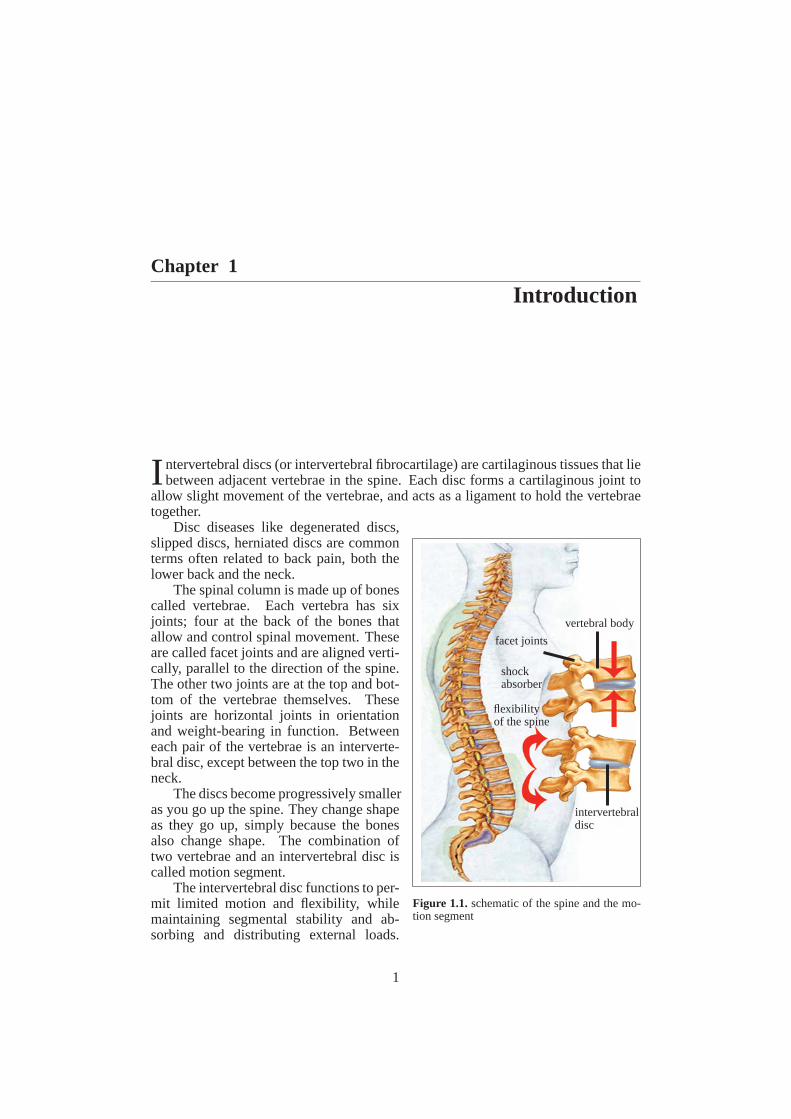
I ntervertebral discs (or intervertebral fibrocartilage) are cartilaginous tissues that liebetween adjacent vertebrae in the spine. Each disc forms a cartilaginous joint to
allow slight movement of the vertebrae, and acts as a ligament to hold the vertebraetogether.
intervertebraldisc
vertebral body
facet joints
flexibilityof the spine
shockabsorber
Figure 1.1.schematic of the spine and the mo-tion segment
Disc diseases like degenerated discs,slipped discs, herniated discs are commonterms often related to back pain, both thelower back and the neck.
The spinal column is made up of bonescalled vertebrae. Each vertebra has sixjoints; four at the back of the bones thatallow and control spinal movement. Theseare called facet joints and are aligned verti-cally, parallel to the direction of the spine.The other two joints are at the top and bot-tom of the vertebrae themselves. Thesejoints are horizontal joints in orientationand weight-bearing in function. Betweeneach pair of the vertebrae is an interverte-bral disc, except between the top two in theneck.
The discs become progressively smalleras you go up the spine. They change shapeas they go up, simply because the bonesalso change shape. The combination oftwo vertebrae and an intervertebral disc iscalled motion segment.
The intervertebral disc functions to per-mit limited motion and flexibility, whilemaintaining segmental stability and ab-sorbing and distributing external loads.
1
2 Chapter 1. Introduction
In fact, the intervertebral discs are fibrocartilaginous cushions serving as the spine’sshock absorbing system, which protect the vertebrae, brain, and otherstructures (i.e.nerves). The discs allow some vertebral motion: extension and flexion. Individualdisc movement is very limited period however considerable motion is possible whenseveral discs combine.
spinal cord
nucleuspulposus
annulusfibrosus
vertebra
nerve root
articularprocess
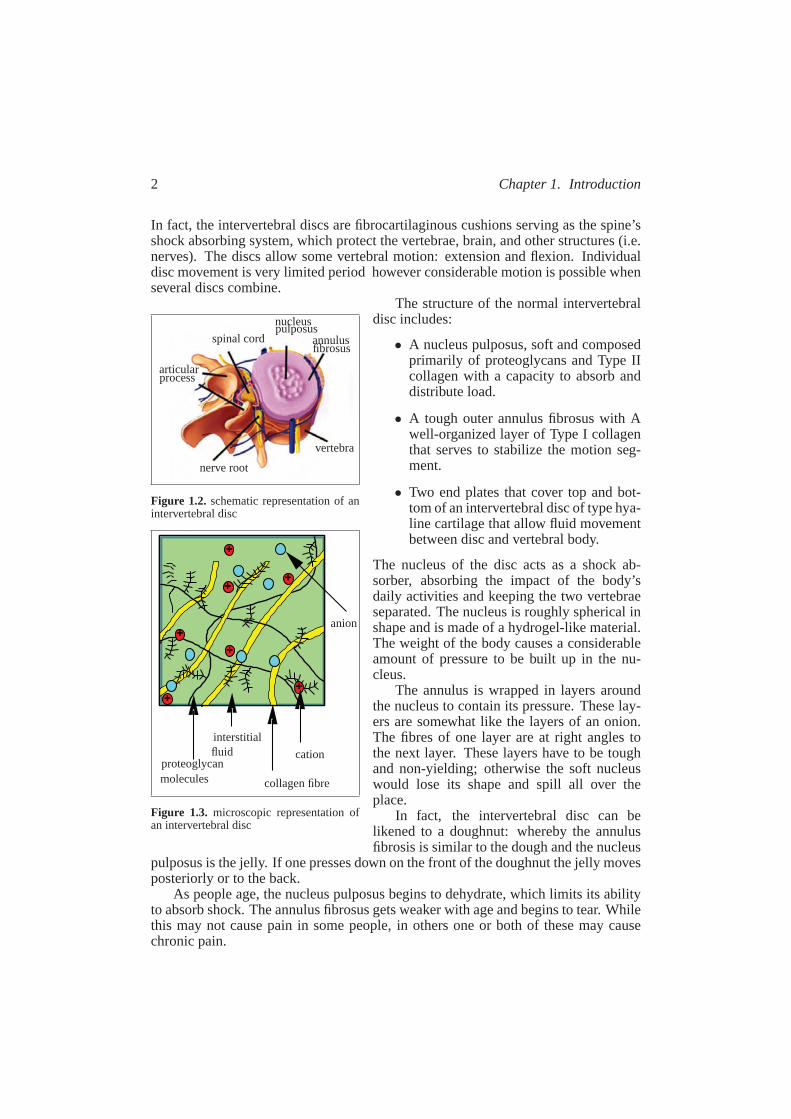
Figure 1.2. schematic representation of anintervertebral disc
+
+
+
+
+
+
++
+
+
+
+
++
anion
cation
interstitialfluid
collagen fibre
proteoglycanmolecules
Figure 1.3. microscopic representation ofan intervertebral disc
The structure of the normal intervertebraldisc includes:
• A nucleus pulposus, soft and composedprimarily of proteoglycans and Type IIcollagen with a capacity to absorb anddistribute load.
• A tough outer annulus fibrosus with Awell-organized layer of Type I collagenthat serves to stabilize the motion seg-ment.
• Two end plates that cover top and bot-tom of an intervertebral disc of type hya-line cartilage that allow fluid movementbetween disc and vertebral body.
The nucleus of the disc acts as a shock ab-sorber, absorbing the impact of the body’sdaily activities and keeping the two vertebraeseparated. The nucleus is roughly spherical inshape and is made of a hydrogel-like material.The weight of the body causes a considerableamount of pressure to be built up in the nu-cleus.
The annulus is wrapped in layers aroundthe nucleus to contain its pressure. These lay-ers are somewhat like the layers of an onion.The fibres of one layer are at right angles tothe next layer. These layers have to be toughand non-yielding; otherwise the soft nucleuswould lose its shape and spill all over theplace.
In fact, the intervertebral disc can belikened to a doughnut: whereby the annulusfibrosis is similar to the dough and the nucleus
pulposus is the jelly. If one presses down on the front of the doughnut the jelly movesposteriorly or to the back.
As people age, the nucleus pulposus begins to dehydrate, which limits its abilityto absorb shock. The annulus fibrosus gets weaker with age and beginsto tear. Whilethis may not cause pain in some people, in others one or both of these may causechronic pain.
1.1. Existing models for swelling of intervertebral discs 3
Historically, Hippocrates (460-390 BC) is the father of spine surgery (Marketosand Skiadas, 1999a). Galen (129-210 AD) compiled treaties of orthopedic treatmentslike: experimental physiologist and made many true observations on how the bodyworks. Galen described four spinal suffering, kyphosis, lordosis,scoliosis and seisisthat occur due to tuberculosis nodes on the lungs, falls on to the hips or shoulders,aging and painful conditions (Marketos and Skiadas, 1999b).
The main structures of annulus fibrosus are a fibre network consist of collagenfibres and proteoglycan molecules, freely moving charged particles (Na+ and Cl−)and an interstitial fluid.
The large proteoglycan molecules consisting of a protein core to which up to 100highly sulphated glycosaminoglycan chains (GAGs) are attached. A distinctive fea-ture of glycosaminoglycan chains is their high number of charges. The concentrationof these fixed charges is called the fixed charge density.Because of the entanglement of the glycosaminoglycans in the collagen network, thecharges of proteoglycans are fixed in the tissue, unlike the small ions like Na+ andCl−.
The main function of the intervertebral disc is mechanical. The disc transmitsload along the spinal column and also allows the spine to bend and twist. The loadson the disc arise from body weight and muscular activity, and change with posture.
Discs are under pressure, which varies with posture from around 0.1 to0.2 MPaat rest, to around 1.5 to 2.5 MPa while bending and lifting. The pressure is mainlydue to water pressure across the nucleus and inner annulus in a normal disc.
In fact, intervertebral discs exhibits swelling and shrinking behaviour which iscaused by mechanical force(weight of the body), chemical force (changing the saltconcentration) and electrical force (electrical potential field). In all cases the swellingis caused by inflow or outflow of fluid.
The fixed charge density is an important determinant of the swelling properties(osmotic pressure) of the intervertebral disc.
1.1 Existing models for swelling of intervertebral discs
Modelling the mechanical and electro-chemical behaviour of soft tissues such as in-tervertebral disc is an essential task in improving the understanding of failure mecha-nisms. Several researchers have posed sets of equations which present the mechanicaland/or electro-chemical behaviour of such tissues.
We distinguish between the components and the phases in this way that the com-ponents are considered to be continua related to the same macroscopic volumemea-sure for all components (in our case a solid, a liquid, anions, and cations), and phasesare continua related to their own real volume measure (in our case solid and fluid).Mixture theory (Bowen, 1980) is a framework, in which the model integratesmechan-ical deformations and loads, diffusion, convection and chemical reactions of differentsolutes. Theories that describe the mechanical behaviour of cartilaginous tissues canbe divided into three categories:
• An earlier study from geomechanics presents two-component models (bipha-sic), that describe the solid-fluid interactions.((Biot, 1941) and (Biot, 1972))
4 Chapter 1. Introduction
These models do not consider the electrical charge and therefore cannot de-scribe osmotic effects, which have a major influence on the swelling behaviourof tissues.
• Osmotic effects are modelled in a triphasic model (Lai et al., 1991) and (Guet al., 1997) that take into account the ionic effects. In the triphasic model threephases are defined: a charge porous solid phase (collagen fibers and proteogly-cans), the interstitial fluid phase, and the fluid miscible phase (the ionic phase).The triphasic model extends the biphasic model using physico-chemical the-ory.
• In the four-component mixture theory (Huyghe and Janssen, 1997) a deformableand charged porous medium is saturated with a fluid with dissolved cations andanions. In fact, the four component model takes the geometric non-linearity,electrical fluxes and potential gradient into account. By introducing the elec-tronegativity as a restriction on the second law of thermodynamics, electricalphenomena are modelled.
1.2 Finite element analysis for the numerical solution
The governing equations for the two-component model form a linear time-dependentsystem, involving solid displacement, fluid pressure and fluid flow.
In the case of a four-component model we are dealing with a nonlinear time-dependent system, involving solid displacement, liquid and ions potentials, liquidflow and ions flow, 15 equations and unknowns in a three-dimensional configuration.
Of the various forms of discretisation which are possible, one of the most usedis the finite difference process. Another method that is often used in many physicalapplications is concerned with various trial function approximations falling underthe general classification of finite element methods. It has been shown thatevenfinite difference processes can be included as a subclass of this more general theory(Ciarlet, 1978).
The name “mixed method” is applied to a variety of finite element methods thathave more than one approximation space. Typically one or more of the spaces playthe role of Lagrange multipliers to enforce constraints. The name and many oftheoriginal concepts for such methods originated in solid mechanics where it was de-sirable to have a more accurate approximation of certain derivatives of displacement.However, for the Stokes equations that govern viscous fluid flow, the natural Galerkinapproximation is a mixed method (Brezzi, 1974), (Fortin, 1977) and (Brezzi andFortin, 1991).
In fact, mixed method involves the independent interpolation of a kinematic quan-tity, such as displacement, and a kinetic one, such as flow. Hybridization is a specialclass of mixed method. In fact, it is differentiated from mixed method because thekinetic variables are forced to satisfy an equilibrium relation. Because of the ad-ditional interpolation of the kinetic variable, mixed and hybrid methods generallyrequire somehow more computational effort to implement at the element level thando standard methods. However this effort is well justified by the flexibility to spec-
1.3. Aims and contents of this thesis 5
ify independently the interpolation functions representing the kinetic variables withinthe element, as compared to conventional methods for which the kinetic variables arerepresented as derivatives of the kinematic ones.
1.3 Aims and contents of this thesis
In chapter 2 we give a historical overview of the mixture theory. Then stepby stepwe construct the four-component mixture model for the swelling of tissues.We firstpresent the kinematic consideration and the balance laws. Then the constitutive equa-tions are derived. We present the set of field equations for the Lagrangian descriptionfor the four-component system. In some detail, the transformation of the equations tothe reference configuration of the skeleton is discussed. The infinitesimaldeforma-tion assumption for the solid skeleton simplifies the equations. It is shown that thismodel in the absence of ions reduces to a two-component system.
To verify the numerical solutions for this model we need to derive a set of an-alytical solutions for the reduced system of equations. Chapter 3 is devoted to thisfact. We set ourselves the task of deriving a set of analytical solutions for the one-dimensional four-component model. We derive the analytical solutions forthe two-component mixture model which is simpler and then generate the solution for thefour-component model.
In chapter 4, the two-component model is considered. In our model it is desirableto obtain approximations of the fluid flow and ions flow that fulfil the conservationequations. In finite element simulations, these quantities are generally calculated bydifferentiation of the electro-chemical potential solutions. This approach may leadto violation of the mass conservation principle. We propose a mixed formulation forthe two-component mixture. The existence and uniqueness for the solution of thediscretised system is proven. We introduce the mixed hybrid technique. Althoughthe hybridization method reduces the number of degrees of freedom, in the compu-tations we only have to compute inverses of element-wise block diagonal matrices.The derived algorithms are tested for two type of examples: a one-dimensional con-solidation experiment and a two-dimensional footing problem. The results forthefirst problem is verified with the analytical solutions derived in chapter 3.
In chapter 5, the mixed variational formulation for the four-component model isconsidered. The existence and uniqueness after discretisation in spaceand time forthe solution of the linearised system is proven. Using the MHFEM technique forour model, we still have an indefinite system but the advantage is that the numberof degrees of freedom will be reduced. In fact, for a three-dimensional problem thisnumber will be reduced from 15 to 6 degrees of freedom.
References
Biot, M. A.: 1941, ‘General theory of three-dimensional consolidation’.Journal ofApplied Physics.12, 155–164.
Biot, M. A.: 1972, ‘Theory of finite deformation of porous solids’.Indiana Univer-sity Mathematical Journal.21, 597–620.
6 Chapter 1. Introduction
Bowen, R. M.: 1980, ‘Incompressible porous media models by use of the theory ofmixtures’. Int. J. Engng. Sci.III 18 , 1129–1148.
Brezzi, F. : 1974, ‘On the existence, uniqueness and approximation of saddle-pointproblems arising from Lagrangian multipliers.’RAIRO. Anal. Numer.47, 217–235.
Brezzi, F., Fortin. M.: 1991,Mixed and Hybrid Finite Element Methods.Springer-Verlag, Berlin-heidelberg-New York.
Ciarlet, P. G. : 1978,The Finite Element Method for Elliptic Problems.Studies inMathematics and Its Applications4 (North Holland, Amsterdam).
Fortin, M: 1977, ‘An analysis of the convergence of mixed finite element methods.’RAIRO. Anal. Numer.11, 341–354.
Lai, W. M., Hou, J. S., Mow., V. C. : 1991, ‘A triphasic theory for the swelling anddeformation behaviours of articular cartilage.‘ASME Journal of BiomechanicalEnginnering113, 245–258.
Gu, W. Y., Lai, W. M., Mow, V. C.: 1997, ‘A triphasic analysis of negative osmoticflows through charged hydrated soft tissues’.J. Biomechanics.30, 71–78.
Huyghe, J. M., Janssen, J. D. : 1997, ‘Quadriphasic mechanics of swelling incom-pressibleporous media.‘Int. J. Engng. Sci.35, 793–802.
Marketos, S. G., Skiadas P.: 1999, ‘Hippocrates : The father of spine surgery’. Spine.24, no13, 1381–1387.
Marketos, S. G., Skiadas P.: 1999, ‘Galen: A pioneer of spine research’. Spine.24,no22, 2358–2362 .
Chapter 2
Thermodynamic modelling of deformablesaturated porous media
⋆
I n many branches of engineering, for example, in chemical engineering, materialscience, and soil mechanics, as well as in biomechanics, the reactions of material
systems undergoing external or internal loading must be studied and described pre-cisely in order to be able to predict the responses of these systems. Subsequently,the most important point of the investigation is to determine the composition of thebody, because one must know the physically and chemically differing materials thatconstitute the system under consideration. The material systems in these fieldsofengineering can be composed in various ways. Solids can contain closed and openpores. The pores can be filled with fluids and, due to the material propertiesof thesolids and the motions of the fluids, there are maybe interaction between the con-stituents.
Because the exact description of the locations of the pores (empty or filled withfluids) and the solid material is practically impossible, the heterogeneous compositioncan be investigated using the volume fraction concept. This concept resultsin theeffect that “smeared” substitute continua with reduced densities for the solid andfluid phases arise which can then be treated by the mixture theory.
Reflections on the fundamentals of mechanics, which were already formulated toa great extent in the eighteenth and nineteenth centuries, have been considered in thelast decades, beginning in the 1950s. These results form the basis of modern con-tinuum mechanics, which makes a consistent treatment of gaseous, liquid, and solidbodies possible. Modern continuum mechanics was essentially formed by Truesdell.In two books (Truesdell and Toupin, 1960) and (Truesdell and Noll, 1965) and innumerous articles, he and his disciples laid down their ideas and created a closedcontinuum theory. However, their work is not undisputed.
Moreover, Truesdell was the scientist who reformulated and extended the mixturetheory. After the fundamental work of Stefan, Duhmen, Gibbs, Raynolds, Jaumann,and Lohr, it was Truesdell (Truesdell, 1957) who introduced local balance equations
⋆ Parts of this chapter will be appeared in ESAIM: Mathematical Modelling andNumerical Analysis(Malakpoor et al., 2006)
7
8 Chapter 2. Thermodynamic modelling of deformable saturated porous media
for mass, momentum, and energy of arbitrary constituted mixtures. These balanceequations are referred to the individual constituents in consideration of all couplingterms. Truesdell used as a basis of his derivations certain principles, which later havebeen adopted as so-called “metaphysical principles”:
1 All properties of the mixture must be mathematical consequences of propertiesof the constituents.
2 So as to describe the motion of a constituent, we may in imagination isolate itfrom the rest of the mixture, provided we allow properly for the actions of theother constituents upon it.
3 The motion of the mixture is governed by the same equations as is a singlebody.
In Truesdell’s description of mixtures (Truesdell and Toupin, 1960), both a properstatement for the moment of momentum balance equation and a generalization of theentropy inequality for mixtures were missing. With respect to Truesdell’s mixturetheory, (Kelly, 1964) developed distinct balance laws on the basis of onefundamentalbalance equation, thus allowing a clear assignment of the effects resulting from thepartial balance equations to the mechanical quantities of the mixture. Concerning themoment of momentum balance, Kelly proposed moment of momentum supply terms,thus admitting unsymmetrical partial stress tensors.
In the early 1960s, a thermodynamic approach to the constitutive theory wasgenerally unknown, until (Coleman and Noll, 1963) as well as (Coleman andMizel,1964) introduced the development of thermodynamic restrictions from the entropy in-equality. This application of the entropy inequality to heterogeneous materials causedexceptional difficulties.
It was later pointed out that the entropy inequality postulated by (Bowen, 1967)was the first correct version of the entropy inequality for mixtures. The developmentof the mixture theory was brought to an end to a certain extent already in the early1970s, namely in so far as the fundamentals developed up to that time have remainedvalid up to today.
In the theory of mixtures (Bowen, 1976), one porous solid skeleton andk − 1miscible or immiscible pore-fluids are considered. The motivations and examplesofmixtures can be found in many branches of science and engineering, like the investi-gation of the coupled solid deformation and pore-fluid flow behaviour in geoscience,the well-known consolidation problem of soil mechanics, in applications concerningthe exploitation of natural gas and oil reservoirs, or in biomechanical problems likethe investigation of swelling and shrinking of cartilaginous tissues or intervertebraldisks, which is the main item of this work. For the case of saturated porous media, themain idea is the representation of a saturated porous medium as the superposition, intime and space, of two continua or phases; the first representing the skeleton phase,the second the fluid phase. The fluid volume fraction of a given volume is the ratioof the non-solid volume to the total volume and is denoted byϕf .
As mentioned above, in the theory of mixture there is no measure to get any mi-croscopic information. Therefore it is convenient to combine the theory ofmixtures

9
with the concept of volume fractions. By this procedure, basically definingthe the-ory of porous media, one can find an excellent tool for the description ofgeneralimmiscible multiphasic aggregates, where the volume fractions are the measures ofthe local portions of the individual phases of the overall medium.
It seems that Morland (Morland, 1972) was the first scientist to use the volumefraction concept in connection with the mixture theory. In 1966, however,Mills(Mills, 1966) had already used the volume fraction concept for incompressible mix-tures of two separated Newtonian fluids. In this article, Mills also formulated theincompressibility condition in such a way that he assumed the real densities of bothconstituents to be constant, i.e., that the sum of the volume fractions was equalto one.In the volume fraction concept, it is assumed that the porous solid always models acontrol space and that only liquids contained in the pores can leave the control space.
The basis of the description of porous media, using elements of the theory ofmix-tures restricted by the volume fraction concept, is the model of a macroscopicbody,where neither a geometrical interpretation of the pore structure nor the exact loca-tion of the individual components of the body (constituents) are considered (Ehlers,2002), (Hassanizadeh, 1986a) and (Hassanizadeh, 1986b). We proceed from the as-sumption that the constituents are “smeared” over the control space that is shapedby the porous solid, i.e., that each substitute constituent occupies the total volume ofspace simultaneously with the other constituents.
In this chapter, we consider a continuously deformable saturated porousmedium.This type of saturated porous media can be observed in numerous solid mechanicsproblems and is studied since many years in civil engineering. It is also studied inbiomechanics to model the coupling between fluid flow and mechanical loading incartilage or skin.
Many biological porous media exhibit swelling and shrinking behaviour when incontact with salt concentrations. This phenomenon, observed in cartilageand gels, iscaused by electric charges fixed to the solid, counteracted by corresponding chargesin fluid. These charges result in a variety of features, including swelling,electro-osmosis, streaming potentials and streaming currents. We distinguish between thecomponents and the phases in this way that the components are considered tobecontinua related to the same macroscopic volume measure for all components (inourcase a solid, a fluid, anions, and cations), and phases are continua related to their ownreal volume measure (in our case solid and fluid). Mixture theory (Bowen,1980)is a framework, in which the model integrates mechanical deformations and loads,diffusion, convection and chemical reactions of different solutes.
An earlier study from geomechanics presents biphasic models, that describe thesolid-fluid interactions. These models can not describe osmotic effects, which havea major influence on the behaviour of tissues. Osmotic effects are modelled in atriphasic model (Lai et al., 1991) and (Gu et al., 1997) and in a four-componentmixture theory (Huyghe and Janssen, 1997), (Frijns, 2001) and (Chen et al., 2006).In the four-component mixture theory a deformable and charged porousmedium issaturated with a fluid with dissolved cations and anions.
The solid skeleton and fluid are assumed to be intrinsically incompressible andtherefore a non-zero fluid flux divergence gives rise to swelling or shrinkage of theporous medium. Alternatively, a gradient in fluid pressure, ion concentrations or

10 Chapter 2. Thermodynamic modelling of deformable saturated porous media
voltage results in flow of the fluid and ions (Frijns, 2001).In this chapter, we construct the model of four-component porous material in
Lagrangian coordinates of the skeleton. Such a description, particularlyuseful incomputer-aided solutions, has not been used yet for multi-phase systems where theskeleton is usually described in Eulerian coordinates.
This chapter is outlined as follows. In the next two sections, we present thekine-matic consideration and the balance laws. Section 3 is devoted to constitutive equa-tions. In section 4 we present the set of field equations for the Lagrangian descriptionfor the four-component system. In some detail, the transformation of the equations tothe reference configuration of the skeleton is discussed. The sixth section is devotedto the Donnan equilibrium and boundary conditions. In section 7 we assume an in-finitesimal deformation for the solid skeleton and we derive the simplified equations.In section 8 we present the reduction to a two-component system.
2.1 Kinematic
The swelling and shrinking behaviour of cartilaginous tissues (like intervertebraldisc) can be modelled by a four- component mixture theory in which a deformableand charged porous medium is saturated with a fluid with dissolved ions. Within theconcept of mixture theory, we consider a porous solid skeleton and an immisciblepore-fluid. The idea is to present the saturated porous medium as a superposition ofdeformable phases that occupy the same domain in the three-dimensional space attime t. In other words, we assume that different phases exist simultaneously at eachpoint in space. Cartilaginous tissues are assumed to consist of two phases, a solidphase and a fluid phase. In cartilaginous tissues, the fluid phase consistsof threecomponents: liquid, cation and anion. We use the abbreviations andf respectivelyfor the solid phase and the fluid phase. The symbolsl, + and− stand for liquid,cation and anion, respectively (cf. Figure 2.1).
+
+
+
+
+
+
++
+
+
+
+
id
io n s
anions
microstructure continuum modelvolume fractionsanionscationscations
fluid
solidsolid
Figure 2.1.Micro-structure and macroscopic model
Definition 2.1. A bodyΩ is a set whose elements can be put into bijective correspon-dence with the points of a regionΩ of a Euclidean point space. The elements ofΩ arecalled particles andΩ is referred to as a configuration ofΩ; the point inΩ to whicha given particle ofΩ corresponds is said to be occupied by that particle.
2.1. Kinematic 11
P α, P β
P α
P αP β
P β
Xα
Xβx
(t0)
(t)
(τ > t)χα(t)
χβ(t)
O
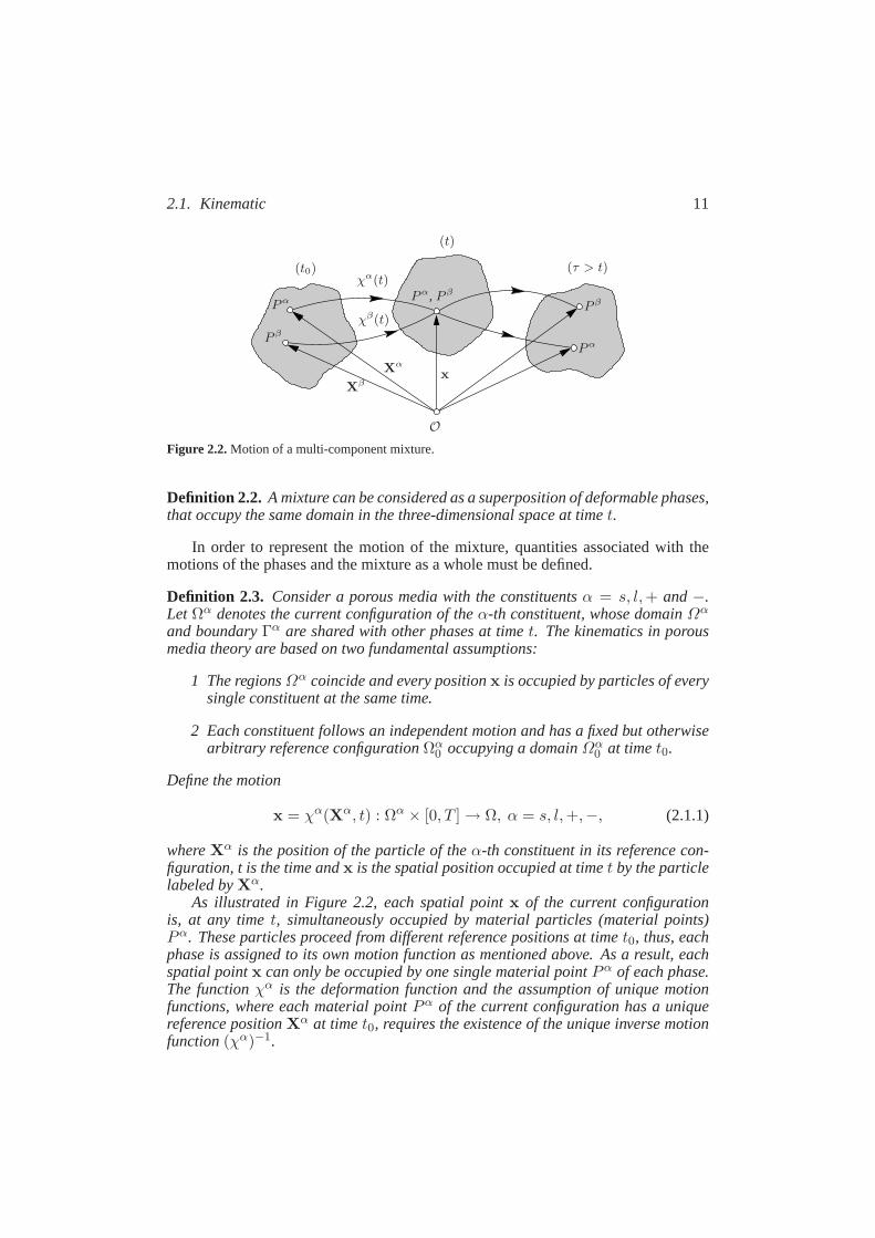
Figure 2.2.Motion of a multi-component mixture.
Definition 2.2. A mixture can be considered as a superposition of deformable phases,that occupy the same domain in the three-dimensional space at timet.
In order to represent the motion of the mixture, quantities associated with themotions of the phases and the mixture as a whole must be defined.
Definition 2.3. Consider a porous media with the constituentsα = s, l,+ and−.Let Ωα denotes the current configuration of theα-th constituent, whose domainΩα
and boundaryΓα are shared with other phases at timet. The kinematics in porousmedia theory are based on two fundamental assumptions:
1 The regionsΩα coincide and every positionx is occupied by particles of everysingle constituent at the same time.
2 Each constituent follows an independent motion and has a fixed but otherwisearbitrary reference configurationΩα
0 occupying a domainΩα0 at timet0.
Define the motion
x = χα(Xα, t) : Ωα × [0, T ] → Ω, α = s, l,+,−, (2.1.1)
whereXα is the position of the particle of theα-th constituent in its reference con-figuration, t is the time andx is the spatial position occupied at timet by the particlelabeled byXα.
As illustrated in Figure 2.2, each spatial pointx of the current configurationis, at any timet, simultaneously occupied by material particles (material points)Pα. These particles proceed from different reference positions at timet0, thus, eachphase is assigned to its own motion function as mentioned above. As a result, eachspatial pointx can only be occupied by one single material pointPα of each phase.The functionχα is the deformation function and the assumption of unique motionfunctions, where each material pointPα of the current configuration has a uniquereference positionXα at timet0, requires the existence of the unique inverse motionfunction(χα)−1.
12 Chapter 2. Thermodynamic modelling of deformable saturated porous media
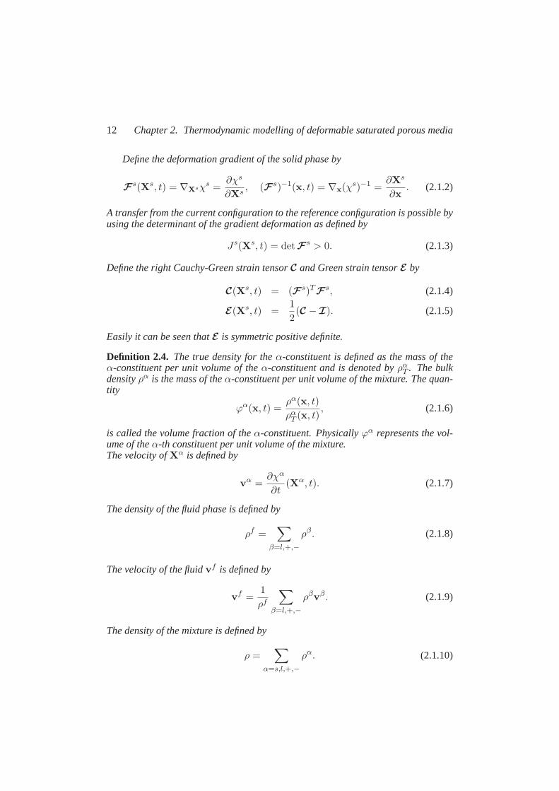
Define the deformation gradient of the solid phase by
Fs(Xs, t) = ∇Xsχs =
∂χs
∂Xs, (Fs)−1(x, t) = ∇x(χs)−1 =
∂Xs
∂x. (2.1.2)
A transfer from the current configuration to the reference configuration ispossible byusing the determinant of the gradient deformation as defined by
Js(Xs, t) = detFs > 0. (2.1.3)
Define the right Cauchy-Green strain tensorC and Green strain tensorE by
C(Xs, t) = (Fs)TF
s, (2.1.4)
E(Xs, t) =1
2(C − I). (2.1.5)
Easily it can be seen thatE is symmetric positive definite.
Definition 2.4. The true density for theα-constituent is defined as the mass of theα-constituent per unit volume of theα-constituent and is denoted byρα
T . The bulkdensityρα is the mass of theα-constituent per unit volume of the mixture. The quan-tity
ϕα(x, t) =ρα(x, t)
ραT (x, t)
, (2.1.6)
is called the volume fraction of theα-constituent. Physicallyϕα represents the vol-ume of theα-th constituent per unit volume of the mixture.The velocity ofXα is defined by
vα =∂χα
∂t(Xα, t). (2.1.7)
The density of the fluid phase is defined by
ρf =∑
β=l,+,−
ρβ . (2.1.8)
The velocity of the fluidvf is defined by
vf =1
ρf
∑
β=l,+,−
ρβvβ . (2.1.9)
The density of the mixture is defined by
ρ =∑
α=s,l,+,−
ρα. (2.1.10)
2.2. Balance equations 13
The velocity of the mixturev is defined by
v =1
ρ
∑
α=s,l,+,−
ραvα. (2.1.11)
If Ψ is any scalar function ofx and t, the derivatives ofΨ following the motiongenerated byv andvα are, respectively,
DΨ
Dt=
∂Ψ
∂t+ ∇Ψ · v, (2.1.12)
DαΨ
Dt=
∂Ψ
∂t+ ∇Ψ · vα. (2.1.13)
2.2 Balance equations
In mixture theory and porous media theory, balance equations like balance of mass,balance of momentum, and moment of momentum, as well as balance of energy mustbe established for each constituent in consideration of all interactions andexternalagencies. This means that all quantities resulting from long- and short-range effectsthat influence the individual constituents, as well as the interaction effectsbetweenthe constituents, have to be considered in the balance equations.
Before stating the balance and constitutive equations in the next section, wecon-sider the following assumptions:
1. The mixture is incompressible, which means that both fluid and solid are in-compressible. Henceρs
T andρfT are uniform in position and constant in time.
In other words, volumetric changes of the porous medium are taken into ac-count.
2. We assume that no chemical reactions exist between phases and no sources orsinks exist.
3. We neglect the inertia effects and body forces.
4. The process are assumed to be isothermal.
5. The mixture is assumed to be saturated, i.e,
ϕs + ϕf = 1. (2.2.1)
The volume fraction of the ions is neglected compared to those of the solid andthe fluid (dilute solution),
ϕ+ + ϕ− ≈ 0 =⇒ ϕf =∑
β=l,+,−
ϕβ ≈ ϕl. (2.2.2)
14 Chapter 2. Thermodynamic modelling of deformable saturated porous media
6. It is assumed that the solid matrix is entirely elastic and initially isotropic. Theshear stress associated with mixture deformation is assumed to be negligible inthe fluid phase. We assume that the porous medium is initially homogenous andthereforeϕs is initially uniform. For our binary porous mediumϕ = ϕf ≈ ϕl
indicates porosity and note thatϕs = 1 − ϕ.
Conservation of mass for the phasess andf implies
∂ϕα
∂t+ ∇ · (ϕαvα) = 0, α = s, f. (2.2.3)
Summing up these two equations forα = s, f , and using the saturation assumption(2.2.1), the incompressibility constraint condition reads
∇ ·(ql + vs
)= 0, (2.2.4)
where the specific discharge relative to the solid phase is defined by
ql = ϕ(vl − vs
). (2.2.5)
Note that the fluid velocity is a weighted average of the velocity of the liquid andthe velocities of the ions. Since we are interested in the situation in which there arefar more water molecules than ions, we approximate the velocity of the fluid by thevelocity of the liquid,vf ≈ vl.
The conservation of mass for the dissolved ions implies
∂ϕcβ
∂t+ ∇ · (ϕcβvβ) = 0, β = +,−, (2.2.6)
wherecβ is the molar concentration of ionβ per unit fluid volume andvβ is theaverage velocity of ionβ. Define the molar fluxqβ relative to the fluid with
qβ = ϕcβ(vβ − vl). (2.2.7)
After neglecting body forces and inertia effects, the momentum balance takes theform
∇ · σα + πα = 0, α = s, l,+,−, (2.2.8)
whereσα is the partial stress tensor of constituentsα, πα is the momentum interac-tion with constituents other thanα. The momentum balance for the mixture reads
πs + πl + π+ + π− = 0. (2.2.9)
Hence∇ · σ = ∇ · σs + ∇ · σl + ∇ · σ+ + ∇ · σ− = 0, (2.2.10)
2.2. Balance equations 15
whereσ represents the Cauchy stress tensor of the mixture.The balance of moment of momentum requires that the stress tensorσ be sym-
metric. The partial stressesσα are symmetric, if no moment of momentum interac-tion between constituents occurs (a proof can be found in (Bowen, 1976)). In thiswork we shall assume all partial stresses to be symmetric.
Electroneutrality requires
z+c+ + z−c− + zfccfc = 0, (2.2.11)
wherezβ , β = +,−, is the valence of the dissolved ionβ. For a mono-valent salt,z+ = 1 andz− = −1. The superscriptfc stands for fixed charge, i.e. the attachedionic group, thuscfc denotes the molar concentration of the ions attached to he solidskeleton per unit fluid volume.
The conservation of fixed charge reads
∂ϕcfc
∂t+ ∇ · (ϕcfcvs) = 0. (2.2.12)
In order to gain restrictions for constitutive equations, the second law of thermo-dynamics (entropy inequality) has been usefully applied in continuum mechanics,in mixture theory and, in particular, in the theory of porous media. Following theisothermality and incompressibility conditions, the entropy inequality for a unit vol-ume of the mixture reads (Bowen, 1976):
∑
α=s,l,+,−
(−ϕαD
αΨα
Dt+ σα : ∇vα − πα · vα
)≥ 0, (2.2.13)
whereΨα is the free energy density for theα-constituent per unit volume of theα-thconstituent and is defined byϕαΨα = ψα, whereψα is the Helmholtz free energy ofconstituentα per unit mixture volume.
DefineW to be the Helmholtz free energy of the mixture by
W = Js∑
α=s,l,+,−
ψα = Js∑
α=s,l,+,−
ϕαΨα. (2.2.14)
We try to rewrite the entropy inequality (2.2.13) per initial mixture volume. Note that
DsJs
Dt= Js∇ · vs. (2.2.15)
Material time differentiation ofW with respect to the solid motion gives
DsW
Dt= W∇ · vs + Js
∑
α=s,l,+,−
Dsϕα
DtΨα + Js
∑
α=s,l,+,−
ϕαDsΨα
Dt. (2.2.16)
16 Chapter 2. Thermodynamic modelling of deformable saturated porous media
Evidently,DsΨα
Dt=DαΨα
Dt+ ∇Ψα · (vs − vα), (2.2.17)
so,
− Js∑
α=s,l,+,−
ϕαDαΨα
Dt= −
DsW
Dt+W∇ · vs
+ Js∑
α=s,l,+,−
Dsϕα
DtΨα
− Js∑
β=l,+,−
ϕβ∇Ψβ · (vβ − vs).
The definition of the material time derivative in (2.1.13) and the incompressibilityassumption (2.2.3) imply that
Js∑
α=s,l,+,−
Dsϕα
DtΨα
= Js∑
α=s,f,+,−
(Ψα∂ϕ
α
∂t+ Ψα∇ϕα · vs
)
= Js∑
α=s,f,+,−
(Ψα∂ϕ
α
∂t+ Ψα (∇ · (ϕαvs) − ϕα∇ · vs)
)
= −Js∇ · vs∑
α=s,f,+,−
Ψαϕα − Js∑
β=l,+,−
Ψβ∇ ·(ϕβ(vβ − vs)
)
+ Js∑
α=s,l,+,−
Ψα
(∂ϕα
∂t+ ∇ · (ϕαvα)
)
︸ ︷︷ ︸=0
= −W∇ · vs − Js∑
β=l,+,−
Ψβ∇ ·(ϕβ(vβ − vs)
).
Thus
− Js∑
α=s,l,+,−
ϕαDαΨα
Dt=DsW
Dt− Js
∑
β=s,l,+,−
∇ ·(Ψβϕβ(vβ − vs)
)(2.2.18)
By using equations (2.2.8) and (2.2.10) we have
∑
α=s,l,+,−
σα : ∇vα =∑
α=s,l,+,−
σα∇vs +∑
β=l,+,−
σβ : ∇(vβ − vs)
2.3. Constitutive equations 17
= σ∇vs +∑
β=l,+,−
∇ ·(σβ(vβ − vs)
)
−∑
α=s,l,+,−
∇ · σα · vα + vs∑
α=s,l,+,−
∇ · σα
︸ ︷︷ ︸0
= σ∇vs +∑
β=l,+,−
∇ ·(σβ(vβ − vs)
)+
∑
α=s,l,+,−
πα · vα,
(2.2.19)
therefore the entropy inequality with respect to the initial state of porous solidtakesthe following form
−DsW
Dt+ Jsσ : ∇vs − Js
∑
β=l,+,−
∇ ·(K
β · (vβ − vs))≥ 0. (2.2.20)
whereKβ is thechemical potentialtensor per unit mixture volume for theβ-constituentand is defined by
Kβ = ψβ
I − σβ, β = l,+,−. (2.2.21)
2.3 Constitutive equations
Mixture theory (the basis of porous media theory) is closed, i.e., the number of un-known fields is equal to the sum of the balance equations and the constitutiveequa-tions. In porous media theory, therefore, one has to look for additional equationsin order to close the system of field equations by introducing constitutive equa-tions. These equations connect certain mechanical or thermodynamical quantitiesvia material-dependent constants and must be provided with a Lagrange multipliersfor the evaluation in process of the entropy inequality. If the equation in excess isa constraint of the motion, then the Lagrange multiplier will become an unknownreaction force.
However, it is not sufficient to only fulfil the requirement. Rather more gen-eral “principles”, which were developed in continuum mechanics should be fulfilled.They are:
• Principle of material frame-indifference or objectivity, or in some literatureknown as principle of change of observer. This principle states that the re-sponse of any material must be independent of the observer.
• Principle of dissipation. This principle states that the constitutive relationsmust satisfy the reduced entropy inequality (2.2.20) for all values of their ar-guments (Coleman and Noll, 1963).
• Principle of equipresence. (Truesdell and Toupin, 1960). This statesthat if avariable is used in one constitutive relation of a problem, it should be used in
18 Chapter 2. Thermodynamic modelling of deformable saturated porous media
all the constitutive relations for that problem (unless, its presence contradictssome other law or axiom).
Note that the entropy inequality should hold for all mixtures satisfying the balancelaws, incompressibility and electro-neutrality.
Due to the objectivity principle, we refer the current description of the mixture tothe initial state of the porous solid.
Defining volume fractions
Φα = Jsϕα, α = s, l,+,−, (2.3.1)
per unit initial volume, we can rewrite the balance equation (2.2.3) as follows:
DsΦα
Dt+ Js∇ · (ϕα(vα − vs)) = 0, α = s, l,+,−. (2.3.2)
We shall denoteΦf by Φ. By introducing a Lagrange multiplierp for the incom-pressibility constraint (2.2.4), the entropy inequality (2.2.20) takes the form
−DsW
Dt+ Js(σ + pI) : ∇vs + Js(−K
l + pϕI) : ∇(vl − vs)
− Js∑
β=+,−
Kβ : ∇(vβ − vs) + Js(−∇ · Kl + p∇ϕ) · (vl − vs)
− Js∑
β=+,−
∇ · Kβ · (vβ − vs) ≥ 0. (2.3.3)
The electro-neutrality condition (2.2.11) in the initial state takes the following form
Φz+c+ + Φz−c− + zfcϕ0cfc0 = 0. (2.3.4)
It is easy to check that
DsΦcβ
Dt+ Js∇ ·
(ϕcβ(vβ − vs)
)= 0, ∀β = +,−. (2.3.5)
After combining (2.3.4) and (2.3.5), we obtain another constraint for the entropyinequality as:
∑
β=+,−
1
Vβ∇ ·(zβϕβ(vβ − vs)
)= 0. (2.3.6)
Here we use that
Vβcβ =
ϕβ
ϕ, β = l,+,−, (2.3.7)
whereVβ
is the molar volume of the constituentβ, β = l,+,− andcl = c−c+−c−.Herec is the molar concentration of the fluid phase, which is assumed to be uniformand constant.
2.3. Constitutive equations 19
The equation (2.3.6) can be written in another form as:
z+∇ · (q+ + c+ql) + z−∇ · (q− + c−ql) = 0. (2.3.8)
In (2.3.5), the presence of molar volumeVβ
shows a link betweenϕβ andϕcβ . Forthe constitutive equations, our attempt is to introduce them not dependent onϕβ but
onϕcβ. As we will see laterVβ
will help us for this purpose.Introducing the restriction equation (2.3.6) into inequality (2.3.3) by means of a
Lagrange multiplierλ, yields:
−DsW
Dt+ Js(σ + pI) : ∇vs + Js(−K
l + pϕI) : ∇(vl − vs)
+ Js∑
β=+,−
(−K
β +zβλ
Vβϕβ
I
): ∇(vβ − vs)
+ Js(−∇ · Kl + p∇ϕ) · (vl − vs)
+ Js∑
β=+,−
(−∇ · Kβ +
zβλ
Vβ∇ϕβ
)· (vβ − vs) ≥ 0. (2.3.9)
To close the system, we chooseW , σ+pI,−Kl+ϕpI,−Kβ+ zβλ
Vβ ϕ
βI (β = +,−),
−∇·Kl +p∇ϕ and−∇·Kβ + zβλ
Vβ ∇ϕβ (β = +,−) to be the constitutive variables,
i.e., they are functions of a set of independent variables (the constitutivevariables arethus the dependent variables). We choose as independent variables the Green strainE (cf. (2.1.5)), and the Lagrangian forms of the volume fractions of the liquidandthe ionsΦβ , and the relative velocitiesvβs = (Fs)−1(vβ − vs), β = l,+,−. Thus
W = W (E ,Φβ ,vβs), (2.3.10)
σ + pI =1
JsF
sS(E ,Φβ ,vβs)(Fs)T , (2.3.11)
−Kl + pϕI = F
sK
l(E,Φβ ,vβs)(Fs)T , (2.3.12)
−Kβ +
zβλ
Vβϕβ
I = FsK
β(E,Φβ ,vβs)(Fs)T , β = +,−, (2.3.13)
−∇ · Kl + p∇ϕ = Fs ˜K
l
(E,Φβ ,vβs), (2.3.14)
−∇ · Kβ +zβλ
Vβ∇ϕβ = F
s ˜K
β
(E,Φβ ,vβs), β = +,−. (2.3.15)
20 Chapter 2. Thermodynamic modelling of deformable saturated porous media
We apply the chain rule for the time differentiation ofW , hence we have
DsW
Dt=
∂W
∂E:DsE
Dt+
∑
β=l,+,−
∂W
∂Φβ
DsΦβ
Dt+
∑
β=l,+,−
∂W
∂vβs·Dsvβs
Dt
= Fs∂W
∂E(Fs)T : ∇vs − Js
∑
β=l,+,−
∂W
∂Φβ∇ ·(ϕβ(vβ − vs)
)
+∑
β=l,+,−
∂W
∂vβs·Dsvβs
Dt. (2.3.16)
Here we use that
DsE
Dt= (Fs)T∇vs
Fs.
We insert the equation (2.3.16) in (2.3.9). This results into
(Js(σ + pI) − F
s∂W
∂E(Fs)T
): ∇vs −
∑
β=l,+,−
∂W
∂vβs·Dsvβs
Dt
+ Js
(−K
l +
(p+
∂W
∂Φ
)ϕI
): ∇(vl − vs)
+ Js∑
β=+,−
(−K
β +
(zβλ
Vβ
+∂W
∂Φβ
)ϕβ
I
): ∇(vβ − vs)
+ Js∑
β=l,+,−
fβ · (vβ − vs) ≥ 0,
where
f l = −∇ · Kl +
(p+
∂W
∂Φ
)∇ϕ,
fβ = −∇ · Kβ +
(zβλ
Vβ
+∂W
∂Φβ
)∇ϕβ , β = +,−.
It follows from (2.3.10), (2.3.14) and (2.3.15) that
fβ = Fsfβ(E ,Φβ ,vβs), β = l,+,−. (2.3.17)
2.3. Constitutive equations 21
By a standard argument (Coleman and Noll, 1963), (2.3.17) is satisfied if and only if
σ + pI =1
JsF
s∂W
∂E(Fs)T , (2.3.18)
∂W
∂vβs= 0, β = l,+,−, (2.3.19)
Kl =
(p+
∂W
∂Φ
)ϕI, (2.3.20)
Kβ =
(zβλ
Vβ
+∂W
∂Φβ
)ϕβ
I, β = +,−, (2.3.21)
and ∑
β=l,+,−
fβ · (vβ − vs) ≥ 0. (2.3.22)
Equation (2.3.18) shows that the stress of the mixture can be derived fromthe strainenergy functionW minuspI. It can be seen that herep presents the hydrostaticpressure acting on the mixture (Bowen, 1980). Equation (2.3.19) shows that the strainenergy does not depend on the relative velocities. Define the chemical potentialµl
per unit fluid volume and the electro-chemical potentialµβ , β = +,−, per mol ofion β, such that
Kl = ϕµl
I, (2.3.23)
Kβ = ϕcβµβ
I, β = +,−. (2.3.24)
Therefore equations (2.3.20) and (2.3.21) imply that
µl = p+∂W
∂Φ,
µβ = λzβ +∂W
∂ΦβV
β, β = +,−.
(2.3.25)
It has been shown (Huyghe and Janssen, 1997) that the multiplierλ can be interpretedas the electrical potential of the medium multiplied by the constant of Faraday, i.e.,λ = Fξ.
We use the residual inequality (2.3.22) to establish
fβ(E ,Φβ ,0) = 0, β = l,+,−. (2.3.26)
It is natural to refer to the state wherevls = v+s = v−s = 0 as the state of thermo-dynamic equilibrium. Equation (2.3.26) shows that local interaction forces vanish inthis state. In the approximation where the departures from the state∇0Φ
β = 0 (∇0
is the gradient in initial configuration) andvβs = 0, for β = l,+,−, are assumed tobe small, (2.3.17) can be approximated by
fβ =∑
γ=l,+,−
Bβγ(vγ − vs), β = l,+,−, (2.3.27)
22 Chapter 2. Thermodynamic modelling of deformable saturated porous media
where
Bβγ = Fs ∂ f
β
∂vγs(E,Φγ ,0)(Fs)T , β, γ = l,+,−. (2.3.28)
Given (2.3.22) and (2.3.27), we can conclude thatB is a positive symmetric semi-definite matrix.
Substituting (2.3.25) into equation (2.3.27) and using the approximation offβ weget the classical equations of irreversible thermodynamics:
−ϕl∇µl =∑
γ=l,+,−Blγ(vγ − vs),
−ϕβ
Vβ∇µβ =
∑γ=l,+,−B
βγ(vγ − vs), β = +,−.(2.3.29)
As it is assumed in the previous section, we restrict our considerations to isothermal,non-reacting mixtures where the solid phase is homogeneous. For such a mixturethat consists of four-component, the Helmholtz potential is expressed as a sum of anelastic energyWE(E) and a mixing energyW (Φβ) for β = l,+,−, Huyghe andJanssen (1997). Define
W (E,Φ,Φ+,Φ−) = (µl0 +RTc)Φ + µ+
0
Φ+
V+ + µ−0
Φ−
V−
+ RT (Φc−Φ+
V+ −
Φ−
V− )
ln
Φc−Φ+
V+ −
Φ−
V−
Φc− 1
+ RTΓ+ Φ+
V+
(ln
Φ+
ΦcV+ − 1
)
+ RTΓ− Φ−
V−
(ln
Φ−
ΦcV− − 1
)+WE(E). (2.3.30)
In this relation:
- µl0 is the initial electro-chemical potential of the fluid phase,
- µβ0 is the initial electro-chemical potential of ionβ,
- Γβ ∈ (0, 1] is the osmotic coefficient of ionβ, which is uniform and constant,
- c is the molar concentration of the fluid phase, which is assumed to be uniformand constant,
- R is the universal gas constant,
- T is the absolute temperature, which is uniform and constant since the materi-als are assumed to be isothermal.

2.3. Constitutive equations 23
The constitutive equations (2.3.18) and (2.3.29) that fulfil the second law of thermo-dynamics are
σ + pI =1
JsF
s∂W
∂E(Fs)T , (2.3.31)
−ϕβ∇µβ =∑
γ=l,+,−
Bβγ(vγ − vs), β = l,+,−, (2.3.32)
with µl = µl, µβ = µβ/Vβ, (β = +,−).
By using equations (2.3.25) and (2.3.30) we simplify the equations for the electro-chemical potentials
µl = p+∂W
∂Φ= p+ µl
0 +RTc ln
Φc−Φ+
V+ −
Φ−
V−
Φc
+RT
Φ
(Φ+
V+ +
Φ−
V−
)
−RTΓ+Φ+
V+Φ
−RTΓ−Φ−
V−Φ
, (2.3.33)
and
µβ = zβFξ +∂W
∂ΦβV
β= zβFξ + µβ
0 −RT ln
Φc−Φ+
V+ −
Φ−
V−
Φc
+ RTΓβ lnΦβ
ΦcVβ, β = +,−. (2.3.34)
After linearising the logarithm terms and using (2.3.7) we have
µl ≈ p+ µl0 −RT (Γ+c+ + Γ−c−)
µβ ≈ µβ0 + zβFξ +RTΓβ ln
cβ
c, β = +,−.
(2.3.35)
In (Molenaar et .al, 1999) the components of the friction matrix are related to diffu-sion coefficients of fluid and ions and it can be shown that
Bll = ϕ2K−1 − (Bl+ +Bl−), (2.3.36)
Bii = −Bil, i = +,−, (2.3.37)
Bil = −ϕiRT (ViDi)−1, i = +,−, (2.3.38)
B+− = 0, (2.3.39)
24 Chapter 2. Thermodynamic modelling of deformable saturated porous media
whereK is the permeability andDi is the ion diffusion tensor in free water. Manip-ulation of the second equation in (2.3.32) yields
ϕβ(vβ − vs) = −∑
γ=l,+,−
P βγ∇µγ , β = l,+,−, (2.3.40)
withP βγ = ϕβϕγ(B−1)βγ , β, γ = l,+,−.
P = (P βγ)β,γ=l,+,− can be derived as:
P =
K Kϕ+
ϕKϕ−
ϕ
Kϕ+
ϕ
V+D+ϕ+
RT+K
(ϕ+
ϕ
)2
Kϕ+ϕ−
ϕ2
Kϕ−
ϕKϕ+ϕ−
ϕ2
V−D−ϕ−
RT+K
(ϕ−
ϕ
)2
.
(2.3.41)Now by using (2.3.40) we can derive the specific dischargeql and the ion fluxesqi
in terms of the electro-chemical potentialµβ ,
ql = ϕ(vl − vs) = −∑
γ=l,+,−
P lγ∇µγ
= −K
ϕ(∇µl + ϕ+∇µ+ + ϕ−∇µ−)
= −K(∇µl + c+∇µ+ + c−∇µ−), (2.3.42)
and
qβ =ϕβ
Vβ(vβ − vl) =
ϕβ
Vβ(vβ − vs) −
ϕβ
Vβ(vl − vs)
= −1
Vβ
∑
γ=l,+,−
P βγ∇µγ − cβql
= −Dβcβϕ
RT∇µβ , β = +,−. (2.3.43)
The above relations are called the extended Darcy’s law and Fick’s law.Assuming the electro-neutrality (2.2.11), if we put (2.3.35) into (2.3.42) and
(2.3.43), then the extended Darcy’s law and the Fick’s law can be stated in termsof the variablesp, cβ andξ as follow:
ql = −K(∇p− zfccfcF∇ξ
),
qβ = −Dβϕ
(F
RTzβcβ∇ξ + Γβ∇cβ
), β = +,−.
(2.3.44)
2.4. Reformulation in Lagrangian coordinates 25
From physical considerations (Huyghe and Janssen, 1997),µl andµβ are continuouseven if cfc is not. Therefore we choose the electro-chemical potentials to be theprimal variables.
Remark 2.5. Define the activityfβ by
fβ =
(cβ
c
)Γβ−1
, β = +,−. (2.3.45)
Then based on the definition of the electro-chemical potentials and on the electro-neutrality assumption, the secondary variablescβ, p andξ are expressed as
cβ = −1
2zβzfccfc +
1
2
√
(zfccfc)2 +4c2
f+f−exp
µ+ − µ+0 + µ− − µ−0RT
,
(2.3.46)
p = µl − µl0 +RT
(Γ+c+ + Γ−c−
), (2.3.47)
ξ =1
zβF
(µβ − µβ
0 −RT lnfβcβ
c
), β = +,−. (2.3.48)
The ion concentrationscβ are clearly positive. For numerical stability, it is preferableto use the expression for voltage withβ = − if zfc is positive and vice versa.
2.4 Reformulation in Lagrangian coordinates
From now, we omit the superscript ‘s’ from Fs andJs and Ds
Dt . For a scalara, avectora and a tensorT , the following relations hold for gradient and divergenceoperators in the reference configuration and the current configuration (Chadwick,1999, page 59).
F−T∇0a = ∇a,
1
J∇0 · (JF
−1a) = ∇ · a,
1
J∇0 · (JF
−1T ) = ∇ · T .
Define the displacement field in Lagrangian and Eulerian form by
U(X, t) = x(X, t) − X,
u(x, t) = x − X(x, t),
respectively.Let us choose the configurationΩt0 ⊂ R
3 of the solid skeleton at the initialinstant of timet0 as the reference configuration for the Lagrangian description. The

26 Chapter 2. Thermodynamic modelling of deformable saturated porous media
reference configuration need not to be a stress-free configuration.In fact, the stressΠ0 is defined in the reference configuration and obeys the momentum balance
∇0 · Π0 = 0.
Defineϕ0 andϕs0 = 1 − ϕ0 as the initial porosity and the initial volume fraction
of the solid phase, respectively. Recall the Lagrangian form of the balance equationin (2.3.2):
DJϕα
Dt+ J∇ · (ϕα(vα − vs)) = 0, α = s, l,+,−.
It can be easily seen that the above equation is equivalent to
DJϕα
Dt+ ∇0 ·
(JF
−1ϕα(vα − vs))
= 0, α = s, l,+,−.
Forα = s we haveDJϕs
Dt= 0, or ϕsJ = ϕs
0.
whereϕs0 is the solid volume fraction in the reference configuration. This gives
ϕ = 1 − ϕs = 1 −1 − ϕ0
J. (2.4.1)
Forα = l we obtainDJϕ
Dt+ ∇0 ·Q
l = 0, (2.4.2)
whereQ
l = JF−1ql. (2.4.3)
By using definitions (2.2.5), (2.2.7) and equation (2.3.2), we have
DJϕcβ
Dt+ J∇ · (qβ + cβql) = 0, β = +,−.
The ions balance in Lagrangian form takes the following form
DJϕcβ
Dt+ ∇0 · (Q
β + cβQl) = 0, β = +,−, (2.4.4)
whereQ
β = JF−1qβ, β = +,−. (2.4.5)
In the Lagrangian form, (2.2.12) is expressed as
DJϕcfc
Dt= 0, or ϕcfc = ϕ0c
fc0 J
−1, (2.4.6)
2.5. Total set of equations 27
wherecfc0 is the fixed charge concentration in the reference configuration. From
(2.4.1) follows,(ϕJ)−1 = (J − ϕs
0)−1,
therefore
cfc = cfc0 ϕ0(J − ϕs
0)−1. (2.4.7)
Define the first and second Piola-Kirchhoff stress tensors by
Π = JσF−T ,
S = JF−1σF
−T ,
respectively. Then equation (2.2.10) in Lagrangian form takes the following form
∇0 · Π = 0 or ∇0 ·(SF
T)
= 0, (2.4.8)
The constitutive relation (2.3.31) is given by
σ + pI =1
JF∂W
∂EF
T ,
Considering this relation, the second Piola-Kirchhoff stress is expressed by
S = ΠF−T =
∂W
∂E− pJC
−1, (2.4.9)
where the right Cauchy-Green tensorC is defined in (2.1.4).It is easy to check that the Lagrangian form of equations (2.3.42) and (2.3.43) is
Ql = −K(∇0µ
l + c+∇0µ+ + c−∇0µ
−),
Qβ = −
Dβcβϕ
RT∇0µ
β , β = +,−,(2.4.10)
where
K = JF−1KF
−T , (2.4.11)
Dβ
= JF−1Dβ
F−T , β = +,−. (2.4.12)
2.5 Total set of equations
The combination of the deformation of the porous media and the flow of the fluid andions in the Lagrangian description results into the following set of equations:
28 Chapter 2. Thermodynamic modelling of deformable saturated porous media
Balance Equations
∇0 · (SFT ) = 0,DJϕ
Dt+ ∇0 ·Q
l = 0,
DJϕcβ
Dt+ ∇0 · (Q
β + cβQl) = 0, β = +,−,
Constitutive Equations
∂W
∂E− pJC−1 = S,
−K(∇0µl + c+∇0µ
+ + c−∇0µ−) = Q
l,
−D
βcβϕ
RT∇0µ
β = Qβ, β = +,−.
(2.5.1)
2.6 Donnan equilibrium and boundary conditions
In order to solve the above system of equations, we need to pose the boundary con-ditions. This can be achieved by suitably combining the essential conditions for µl,µβ andU and the natural conditions for the normal components ofQ
β , β = l,+,−,andS.Consider the case that the porous medium is in contact with an electro-neutral bathingsolution, given that the pressurepout, the voltageξout and the ion concentrationscout
are known. The bathing solution contains no fixed charges, thusc+out = c−out = cout.Since the electro-chemical potentials are continuous at the boundary,
µlin = µl
out, (2.6.1)
µ+in = µ+
out, (2.6.2)
µ−in = µ−out, (2.6.3)
whereµlout andµβ
out are the electro-chemical potentials in the outer solution. AssumeΓ+
in = Γ−in = Γ andΓ+
out = Γ−out = 1, then the combination of the above relations
and the relations expressed in (2.3.35) provide
µlin = µl
0 + pout − 2RTcout, (2.6.4)
µβin = µβ
0 + Fzβξout +RT lncout
c, β = +,−, (2.6.5)
where,cout, pout andξout are the ions concentration, fluid pressure and the electri-cal potential of the outer solution, respectively. Equation (2.6.5) forβ = +,− in
2.7. Reduction to infinitesimal deformation 29
combination with (2.6.2) and (2.6.3) imply
µ+0 + µ−0 +RT ln
c2out
c2= µ+
out + µ−out = µ+in + µ−in = µ+
0 + µ−0 +RTΓ lnc+inc
−in
c2,
Therefore, we havec2out
c2=
(c+inc
−in
c2
)Γ
. (2.6.6)
Easily we can see that
π = pin − pout = RT(Γ(c+in + c−in) − 2cout
), (2.6.7)
ξin − ξout =RT
Fzβlncoutc
Γ−1
(cβin)Γ, β = +,−, (2.6.8)
In the above relations,π is the osmotic pressure (Richards, 1980) andξin − ξout isthe Donnan voltage between the inner and outer solution. It is also called the Nernstpotential (Gu et al., 1999), (Helfferich, 1962).
Let Ω be an open domain inRn, n = 1, 2, 3, then defineΩT = Ω × (0, T ] forT > 0 and consider the setsΓD
u andΓNu (and similarlyΓD
p andΓNp ) to be two disjoint
open subsets of the total boundaryΓ = ∂Ω, such thatΓDα ∩ΓN
α = ∅ andΓDα ∪ΓN
α = Γfor α = u andp. We assume
measΓDα > 0 for α = u, p. (2.6.9)
From the above statements we can get the following boundary conditions:
Boundary Conditions
U = 0 onΓDu × (0, T ],
µl = µlin onΓD
p × (0, T ],
µ+ = µ+in onΓD
p × (0, T ],
µ− = µ−in onΓDp × (0, T ],
n · (SFT ) = gNu onΓN
u × (0, T ],n ·Ql = 0 onΓN
p × (0, T ],
n ·Q+ = 0 onΓNp × (0, T ],
n ·Q− = 0 onΓNp × (0, T ].
(2.6.10)
2.7 Reduction to infinitesimal deformation
In this section we keep all the assumption from the previous sections, but wealsoassume infinitesimal deformation for the solid phase.
In the infinitesimal theory of elasticity it is assumed that the components of thedisplacement vector and their spatial derivatives are infinitesimal of the first order so

30 Chapter 2. Thermodynamic modelling of deformable saturated porous media
that we neglect products and squares of these quantities in comparison withtheir firstpowers (Fluugge, 1958, page 6). Using this approximation we find the deformationtensor and the strain tensor as
F = I + ∇0U, E =1
2(∇0U + (∇0U)T ), (2.7.1)
whereU = x−X is the displacement vector. Recall equation (2.4.1), since the solidphase is assumed to have infinitesimal deformation, the Taylor linearisation forJ−1
atF = I implies
J−1≈ 1 −
(1
J2
∂J
∂F
)∣∣∣∣
∣∣∣∣∣∣∣∣F=I
: (F − I) = 1 −∇0 · U.
In the above relation, we use the relation (Holzapfel, 2000, page 41)
∂J
∂F= JF
−T . (2.7.2)
Putting the linearised form ofJ−1 into (2.4.1) results into
ϕ = 1 − (1 − ϕ0)(1 −∇0 · U). (2.7.3)
Also remember the relation for fixed charges density in (2.4.7) given by
cfc = cfc0 ϕ0(J − ϕs
0)−1.
From the assumption of infinitesimal elastic deformation for the solid phase, the Tay-lor linearisation for the function(J − ϕs
0)−1 atF = I results into
(J − ϕs0)
−1≈ (1 − ϕs
0)−1 −
(1
(J − ϕs0)
2
∂J
∂F
)∣∣∣∣
∣∣∣∣∣∣∣∣F=I
: (F − I)
=1
ϕ0−
∇0 · U
ϕ20
. (2.7.4)
Hence
cfc = cfc0
(1 −
∇0 · U
ϕ0
). (2.7.5)
We choose a linear elastic material and therefore the elastic energy part is of the form
WE(E) = µsE : E +λs
2(∇0 · U)2, (2.7.6)
whereλs andµs are the Lame stress constants.
2.7. Reduction to infinitesimal deformation 31
In the next step we will rewrite the equations in the infinitesimal deformationregime. Starting from the force balance and the related constitutive equation(2.4.9)we have
∇0 ·
(∂W
∂EF
T
)−∇0 · (pJF
−1) = 0,
or ∇0 ·
(∂W
∂EF
T
)− J∇p = 0,
or ∇0 ·
(∂W
∂EF
T
)− JF
−T∇0p = 0,
By using (2.7.1) the last equation is reduced to
∇0 · (2µsE + λs∇0U) −∇0p+ ∇0 ·((2µsE + λs∇0U)∇0U
T)
+ ∇0UT∇0p−∇0 · U∇0p+ ∇0 · U∇0U
T∇0p = 0.
Assuming infinitesimal deformation for the solid phase, all terms except the first andsecond terms vanish and finally we have
∇0 · (2µsE + λs∇0 · U) −∇0p = 0.
Note that from (2.7.3), we have
Jϕ = (1 + ∇0 · U) (1 − (1 − ϕ0)(1 −∇0 · U)) = ∇0 · U + ϕ0.
The permeabilityK and diffusion tensorsDβ
are considered to be isotropic tensorsrepresented by scalar multiple of the identity. To make the notations simpler, wechange notations according to the following table:
Old notations ∇0 D/Dt Qβ , β = l,+,− U D
β, β = +,− K
New notations ∇ ∂/∂t qβ, β = l,+,− u Dβ, β = +,− K
Table 2.1.New notations for infinitesimal deformation

32 Chapter 2. Thermodynamic modelling of deformable saturated porous media
Now the total set of equations is given by:
Conservation Equations0 = ∇ · σ −∇p,
0 =∂∇ · u
∂t+ ∇ · ql,
0 =∂(∇ · u + ϕ0)c
β
∂t+ ∇ · (qβ + cβql), β = +,−,
Constitutive Equations
σ = 2µsE + λstrE, E =1
2(∇u + (∇uT )),
ql = −K(∇µl + c+∇µ+ + c−∇µ−),
qβ = −Dβ
RTϕcβ∇µβ , β = +,−,
Secondary Equationsϕ = 1 − (1 − ϕ0)(1 −∇ · u)
cfc = cfc0
(1 −
∇ · u
ϕ0
)
cβ = −1
2zβzfccfc+
+1
2
√
(zfccfc)2 +4c2
f+f−exp
µ+ − µ+0 + µ− − µ−0RT
,
p = µl − µl0 +RT (Γ+c+ + Γ−c−) ,
ξ =1
zβF
(µβ − µβ
0 −RT lnfβcβ
c
), β = +,−,
Boundary Conditionsu = 0 onΓD
u × (0, T ],µl = µl
in onΓDp × (0, T ],
µ+ = µ+in onΓD
p × (0, T ],
µ− = µ−in onΓDp × (0, T ],
gNu = n · (σ(u) − p) onΓN
u × (0, T ],n · ql = 0 onΓN
p × (0, T ],
n · q+ = 0 onΓNp × (0, T ],
n · q− = 0 onΓNp × (0, T ].
(2.7.7)
2.8 Reduction to two-component model
In this section, we shall specialise the results from the four-component theory to abinary mixture of a solid and a fluid. By neglecting the ion contributions and theinfluence of all electrically charged particles in the four-component model,the so-
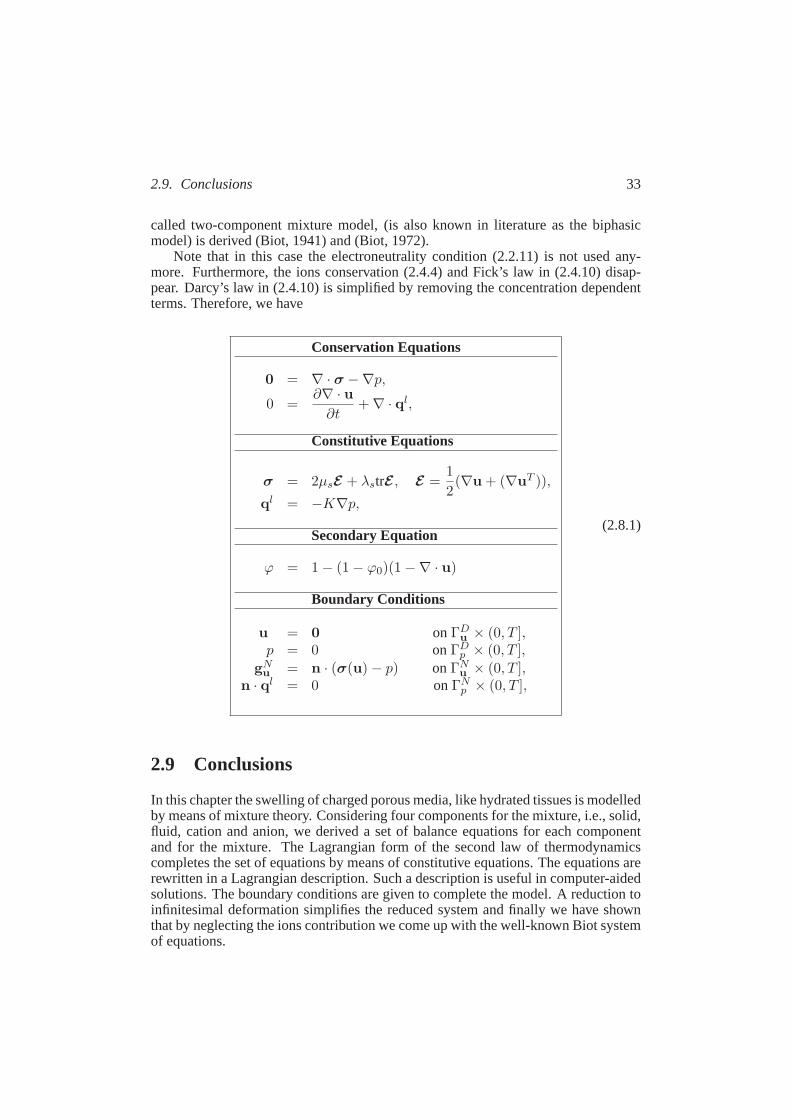
2.9. Conclusions 33
called two-component mixture model, (is also known in literature as the biphasicmodel) is derived (Biot, 1941) and (Biot, 1972).
Note that in this case the electroneutrality condition (2.2.11) is not used any-more. Furthermore, the ions conservation (2.4.4) and Fick’s law in (2.4.10)disap-pear. Darcy’s law in (2.4.10) is simplified by removing the concentration dependentterms. Therefore, we have
Conservation Equations
0 = ∇ · σ −∇p,
0 =∂∇ · u
∂t+ ∇ · ql,
Constitutive Equations
σ = 2µsE + λstrE, E =1
2(∇u + (∇uT )),
ql = −K∇p,
Secondary Equation
ϕ = 1 − (1 − ϕ0)(1 −∇ · u)
Boundary Conditions
u = 0 onΓDu × (0, T ],
p = 0 onΓDp × (0, T ],
gNu = n · (σ(u) − p) onΓN
u × (0, T ],n · ql = 0 onΓN
p × (0, T ],
(2.8.1)
2.9 Conclusions
In this chapter the swelling of charged porous media, like hydrated tissues ismodelledby means of mixture theory. Considering four components for the mixture, i.e.,solid,fluid, cation and anion, we derived a set of balance equations for eachcomponentand for the mixture. The Lagrangian form of the second law of thermodynamicscompletes the set of equations by means of constitutive equations. The equations arerewritten in a Lagrangian description. Such a description is useful in computer-aidedsolutions. The boundary conditions are given to complete the model. A reduction toinfinitesimal deformation simplifies the reduced system and finally we have shownthat by neglecting the ions contribution we come up with the well-known Biot systemof equations.
34 Chapter 2. Thermodynamic modelling of deformable saturated porous media
References
Biot, M. A.: 1941, ‘General theory of three-dimensional consolidation’.Journal ofApplied Physics.12, 155–164.
Biot, M. A.: 1972, ‘Theory of finite deformation of porous solids’.Indiana Univer-sity Mathematical Journal.21, 597–620.
de Boer, R.: 2000,Theory of porous media: Highlights in Historical Developmentand Current State.Springer-Verlag, Berlin.
Bowen, R. M.: 1967, ‘Toward a thermodynamics and mechanics of mixtures’. Art.Rat. Mech. An.24, 370–403.
Bowen, R. M.: 1976, ‘Theory of mixtures’.In Eringen, A. C. (ed.): ContinuumPhysics, Academic Press, New York.III , 1–127.
Bowen, R. M.: 1980, ‘Incompressible porous media models by use of the theory ofmixtures’. Int. J. Engng. Sci.III 18 , 1129–1148.
Bowen, R. M.: 1982, ‘Compressible porous media models by use of the theory ofmixtures’. Int. J. Engng. Sci.20, 697–735.
Chadwick, P.: 1999,Continuum mechanics, concise theory and problems.GeorgeAllen and Unwin, LTD., London.
Chen, Y., Chen, X., Hisada, T.: 2006, ‘Non-linear finite element analysis of mechani-cal electrochemical phenomena in hydrated soft tissues based on triphasic theory.‘Int. J. Numer. Mech. Engng.65, 147–173
Coleman, B. D., Noll, W.: 1963, ‘The thermodynamics of elastic materials with heatconduction and viscosity’.Arch. Rational Mech. Anal.13, 167–178.
Coleman, B. D., Mizel, V. J.: 1964, ‘Existence of caloric equations of state inther-modynamics’.Journal of Chemical Physics.40, 1116–1125.
Coussy, O.: 1995,Mechanics of Porous Continua. Wiley, Chichester.Ehlers, W.: 2002,Foundations of multiphasic and porous materials. In W. Ehlers and
J. Blaum (Eds.):Porous Media: Theory, Expriements and Numerical Applications.Springer-Verlag, Berlin, 3–86.
Flugge, S.: 1958,Handbuch der physik.Elastizitat und plastizitat,(Springer-Verlag)Frijns, A. J. H.: 2001,A four-component mixture theory applied to cartilaginous
tissues. PhD-thesis, Eindhoven University of Technology.Gu, W. Y., Lai, W. M., Mow, V. C.: 1997, ‘A triphasic analysis of negative osmotic
flows through charged hydrated soft tissues’.J. Biomechanics.30, 71–78.Gu, W. Y., Lai, W. M., Mow, V. C.: 1999, ‘Transport of multi-electrolytes in charged
hydrated biological soft tissues’.in Transport in Porous Media.34, 143–157.Hassanizadeh, S. M.: 1986, ‘Derivation of basic equations of mass transport in
porous media, Part 1. Macroscopic balance laws.’Adv. Water Resources9, 196–206.
Hassanizadeh, S. M.: 1986, ‘Derivation of basic equations of mass transport inporous media, Part 2. Generalized Darcy’s and Fick’s laws’.Adv. Water Resources9, 207–222.
Helfferich, F.: 1962,Ion exchange.McGraw-Hill, New York.Holzapfel, G. A.: 2000,Nonlinear Solid Mechanics. Wiley.Huyghe, J. M., Janssen, J. D.: 1997, ‘Quadriphasic mechanics of swelling incom-
pressibleporous media.‘Int. J. Engng. Sci.35, 793–802.Kelly, P. D.: 1964, ‘A reacting continuum’.Int. J. Eng. Sci.2, 129–153.
References 35
Lai, W. M., Hou, J. S., Mow., V. C.: 1991, ‘A triphasic theory for the swellinganddeformation behaviours of articular cartilage.‘ASME Journal of BiomechanicalEnginnering113, 245–258.
Malakpoor, K., Kaasschieter, E. F., Huyghe, J. M. : 2006, ‘Mathematical modellingand numerical solution of swelling of cartilaginous tissues. Part I: Modelingofincompressible charged porous media.’ CASA report, Department of Mathematicsand Computer Science, Technische Universiteit Eindhoven,6-24.
Mills, N.: 1966, ‘Incompressible mixture of Newtonian fluids’.Int. J. Eng. Sci.4,97–112.
Molenaar, M. M., Huyghe, J. M. and Baaijens, F. P. T.: 1999, ‘Constitutive modelingof coupled flow phenomena of fluid, ions and current in shales.’Int. Symp. onCoupled Phenomena in Civil, Mining& Petroleum Engineering, China.
Morland, L. W.: 1972, ‘A simple constitutive theory for a fluid-saturated poroussolid’. J. Geoph. Res.77, 890–900.
Ogden, R. W,: 1997,Non-linear Elastic Deformations. Dover, New York.Richards, E. G.: 1980, ‘An Introduction to physical properties of largemolecules in
solute.’ Cambridge University Press, Cambridge.Truesdell, C.: 1957, ‘Sulle basi della termomeccanicia Rendiconti della RealeAc-
cademianazionale dei Lincei’. R R Ac Naz(8)2233-38, 158–166.Truesdell, C., Toupin, R. A.: 1960, ‘The classical field theories’. In Flugge, S. (ed.):
Handbuch der Physik, III/1 , Springer-Verlag, Berlin, 226–902.Truesdell, C., Noll, W.: 1965, ‘The non-linear field theories of mechanics’. In Flugge,
S. (ed.):Handbuch der Physik, III/3 , Springer Verlag; 3rd edition.Truesdell, C.: 1984, ‘Thermodynamics of diffusion’. In Truesdell, C. (Ed.): Rational
Thermodynamics. 2nd Edition, Springer-Verlag, New York, 219–236.Wilmanski, K,.: 1995, ‘Lagrangian model of two phase porous material.’J. Non.
Equilib. Thermodyn.20, 50–77

Chapter 3
An analytical solution of incompressiblecharged porous media
⋆
Cartilaginous tissues are soft hydrated tissues with strong swelling and shrink-ing properties. This swelling and shrinkage behaviour of cartilaginous tissues
is caused by the flow of water that is bound to the charged solid skeleton of poroustissue. The driving mechanism is an interplay of mechanical, chemical and electricalforces. Swelling and shrinkage can be modelled by a four-component mixture the-ory described in the previous chapter in which the deformable and charged porousmedium is saturated with a fluid with dissolved cations and anions.
The solid skeleton and fluid are assumed to be intrinsically incompressible andtherefore a non-zero fluid flux divergence gives rise to swelling or shrinkage of theporous medium. Alternatively, a gradient in the fluid pressure, ion concentrations orvoltage results in flow of the fluid and ions. To verify the numerical solutions forthis model we need to derive a set of analytical solutions for the reduced system ofequations.
In earlier work (Meerveld et al., 2003), a set of analytical solutions hasbeenderived to verify the finite element solution of model. However, in mass balances(Meerveld et al., 2003, equation 2), the time derivatives of volume fractions are con-sidered instead of their material time derivatives. This can only be done if theLa-grangian coordinate is considered (cf. 2.4). Also the diagonalisation (Meerveld et al.,2003, equation 36) produces complex eigenvalues, therefore the obtained solution se-ries are no longer valid. In fact, the equations in this case are of hyperbolic type.
In this chapter, we set ourselves the task of resolving this problem and deriving aset of analytical solutions for the one-dimensional four-component model. We follow(Terzaghi, 1923) and (Biot, 1956) to derive a coupled system of diffusion equations.This leads to the analytical solutions for the two-component mixture model and thengenerates the solution for the four-component model.
⋆ Parts of this chapter have published inZeitschrift fur Angewandte Mathematik und Mechanik(Malakpoor et al., 2006)
37

38 Chapter 3. An analytical solution of incompressible charged porous media
3.1 Analytical solution for the one-dimensional two-componentmodel
In this section we consider the two-component model of solid and fluid (2.8.1). Thismodel has been widely studied for the consolidation problem (Terzaghi, 1923) and(Biot, 1956). A one-dimensional version of this model reads
Conservation Equations
0 = (2µs + λs)∂2u
∂y2−∂p
∂y,
0 =∂2u
∂t∂y−K
∂2p
∂y2,
Secondary Equation
ϕ = 1 − (1 − ϕ0)(1 −∂u
∂y)
Boundary Conditions
u = 0 onΓDu × (0, T ],
p = 0 onΓDp × (0, T ],
∂u
∂y− p = gN
u onΓNu × (0, T ],
∂p
∂y= 0 onΓN
p × (0, T ].
(3.1.1)
The momentum balance is integrated in the y-coordinate and is equal to
(2µs + λs)∂u
∂y− p = gN
u . (3.1.2)
In an experiment setup, for consolidation an instantaneous load att = t0 is consid-ered (Figure 3.1). Therefore
gNu (t) = −f0H(t− t0) ⇒
∂gNu
∂t= −f0δ(t− t0).
Hence after differentiating (3.1.2) int we have,
(2µs + λs)∂2u
∂t∂y−∂p
∂t= −f0δ(t− t0). (3.1.3)
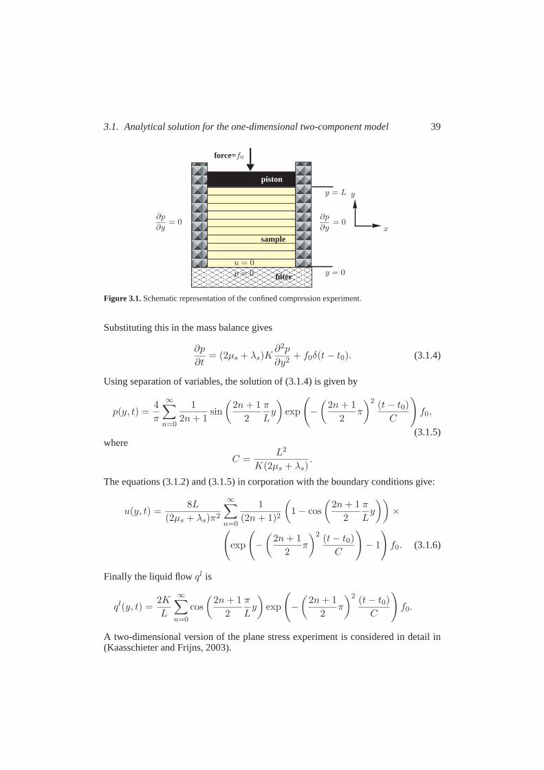
3.1. Analytical solution for the one-dimensional two-component model 39
force=f0
piston
sample
filter
x
y
u = 0
p = 0 y = 0
y = L
∂p
∂y= 0
∂p
∂y= 0
Figure 3.1.Schematic representation of the confined compression experiment.
Substituting this in the mass balance gives
∂p
∂t= (2µs + λs)K
∂2p
∂y2+ f0δ(t− t0). (3.1.4)
Using separation of variables, the solution of (3.1.4) is given by
p(y, t) =4
π
∞∑
n=0
1
2n+ 1sin
(2n+ 1
2
π
Ly
)exp
(−
(2n+ 1
2π
)2 (t− t0)
C
)f0,
(3.1.5)where
C =L2
K(2µs + λs).
The equations (3.1.2) and (3.1.5) in corporation with the boundary conditions give:
u(y, t) =8L
(2µs + λs)π2
∞∑
n=0
1
(2n+ 1)2
(1 − cos
(2n+ 1
2
π
Ly
))×
(exp
(−
(2n+ 1
2π
)2 (t− t0)
C
)− 1
)f0. (3.1.6)
Finally the liquid flowql is
ql(y, t) =2K
L
∞∑
n=0
cos
(2n+ 1
2
π
Ly
)exp
(−
(2n+ 1
2π
)2 (t− t0)
C
)f0.
A two-dimensional version of the plane stress experiment is considered in detail in(Kaasschieter and Frijns, 2003).
40 Chapter 3. An analytical solution of incompressible charged porous media
3.2 Analytical solution for the one-dimensional four-componentmodel
Within the concept of mixture theory, we consider a porous solid skeleton and an im-miscible pore-fluid. As mentioned in the previous chapter, the solid skeleton and fluidare assumed to be intrinsically incompressible. Assuming infinitesimal deformationfor the solid phase, a four-component mixture theory in a Lagrangian description isgiven in which a charged porous media is saturated with a fluid with dissolved cationsand anions (2.7.7).
Following the notations in table 2.1, conservation equations for each constituentimplies
∂Φα
∂t+ ∇ · (ϕαxαs) = 0, α = s, l,+,−, (3.2.1)
wherexαs = JF−1(vα − vs) andΦα = Jϕα.The mass flux is measured per unit of area of the reference configuration for the
solid phase. Equation (3.2.1) forα = s gives
Jϕs = ϕs0, (3.2.2)
whereϕs0 is the initial volume fraction of solid phase. Equation (3.2.2) together with
the saturation assumption implies
ϕf = 1 − ϕs = 1 −1 − ϕf
0
J. (3.2.3)
Since the solid phase is assumed to have infinitesimal deformation, the Taylor lin-earisation forJ−1 atF = I implies
J−1≈ 1 −
(1
J2
∂J
∂F
)∣∣∣∣
∣∣∣∣∣∣∣∣F=I
: (F − I) = 1 −∇ · u,
In the above relation, we useF = I + ∇u and
∂J
∂F= JF
−T . (3.2.4)
After inserting the linearised form ofJ−1 into (3.2.3) we have
ϕf = 1 − (1 − ϕf0)(1 −∇ · u). (3.2.5)
As a consequence of this formula, we have
Φf = ϕf0 + tr E(u). (3.2.6)
Electroneutrality requires
z+c+ + z−c− + zfccfc = 0, (3.2.7)
3.2. Analytical solution for the one-dimensional four-component model 41
wherezβ , β = +,−, is the valence of the dissolved ionβ. The superscript ‘fc’stands for fixed charge, i.e., the attached ionic group, thuscfc denotes the molarconcentration of the attached ions per unit fluid volume.
The conservation of fixed charge in the Lagrangian form reads
ϕfcfc = ϕf0c
fc0 J
−1, (3.2.8)
wherecfc0 is the initial fixed charge concentration. Hence the electroneutrality condi-
tion in the initial state takes the following form
z+Φ+
V+ +
z−Φ−
V− + zfcϕf
0cfc0 = 0. (3.2.9)
Note that
Vβcβ =
ϕβ
ϕf, (3.2.10)
therefore after differentiating in time the electroneutrality condition (3.2.9) canbewritten as:
∑
β=+,−
Fzβ
Vβ
∂Φβ
∂t= ǫ
∂ξ
∂t, (3.2.11)
whereǫ > 0 is a small departure from electroneutrality. In fact, this assumption isneeded for a mathematical reason.
Based on (2.3.32), the constitutive equation to comply the second law of thermo-dynamics is given by
−ϕβ∇µβ =∑
γ=l,+,−
BβγF
T (vγ − vs), β = l,+,−, (3.2.12)
whereµl = µl, µβ = µβ/Vβ, B = (Bβγ)β,γ=l,+,−, is the friction matrix. Based on
(Molenaar et al., 1999),B is defined as
B =
ϕ2
K+ (1 − r)2B++ + (1 − r)2B−− −(1 − r)B++ −(1 − r)B−−
−(1 − r)B++ B++ 0−(1 − r)B−− 0 B−−
,
(3.2.13)and
µl = p+∂W
∂Φ, (3.2.14)
µβ =zβFξ
Vβ
+∂W
∂Φβ, β = +,−. (3.2.15)
42 Chapter 3. An analytical solution of incompressible charged porous media
In the above relation,
Bββ = ϕβRT (VβDβ)−1, β = +,−, (3.2.16)
whereDβ > 0 is the ion diffusion in free water.0 ≤ r ≤ 1 is the hindrance factorand it is assumed to contain all physical phenomena reducing ionic diffusionrate andidentical for cation and anion diffusion.W is the Helmholtz free energy of the porousmedium. For such a mixture that consists of four-component, the Helmholtz energyW is expressed as a sum of elastic energy and a mixing energy forβ-th constituent,β = l,+,−, (2.3.30).
W (E,Φ,Φ+,Φ−) = (µl0 +RTc)Φ + µ+
0
Φ+
V+ + µ−0
Φ−
V−
+ RT (Φc−Φ+
V+ −
Φ−
V− )
ln
Φc−Φ+
V+ −
Φ−
V−
Φc− 1
+ RTΓ+ Φ+
V+
(ln
Φ+
ΦcV+ − 1
)
+ RTΓ− Φ−
V−
(ln
Φ−
ΦcV− − 1
)+WE(E). (3.2.17)
In this relation:
- µl0 is the initial electro-chemical potential of the fluid phase,
- µβ0 is the initial electro-chemical potential of ionβ,
- Γβ ∈ (0, 1] is the osmotic coefficient of cation and anion forβ = +,−, re-spectively which is uniform and constant. Here we assumeΓ+ = Γ− and wedenote it byΓ.
- c is the molar concentration of the fluid phase. Since ion concentrations aresmall,c is assumed to be uniform and constant,
- λs andµs are the Lame stress constants,
- R is the universal gas constant,
- T is the absolute temperature, which is uniform and constant, since the state isassumed to be isothermal,
- WE is the elastic energy and is defined by
WE(E) =λs
2(tr E(u))2 + µsE(u) : E(u). (3.2.18)
3.2. Analytical solution for the one-dimensional four-component model 43
With the prescribed energyW , the relations (3.2.14) and (3.2.15) are postulated as
µl = µl0 + p−RTΓ(c+ + c−), (3.2.19)
µβ = µβ0 +
zβFξ
Vβ
+RTΓ
Vβ
lncβ
c, β = +,−. (3.2.20)
Remark 3.1. It is easy to see that from(3.2.7), (3.2.19)and (3.2.20)we have
cβ = −1
2zβzfccfc +
1
2
√
(zfccfc)2 + 4c2 expV
+(µ+ − µ+
0 ) + V−(µ− − µ−0 )
RTΓ,
(3.2.21)for β = +,−, and
p = µl − µl0 +RTΓ(c+ + c−), (3.2.22)
ξ =V
β
zβF
(µβ − µβ
0 − p−RTΓ
Vβ
lncβ
c
), β = +,−. (3.2.23)
The above formulas will be needed to derive initial and boundary values forcβ, pandξ.
In the following lemma, we will show that the matrixB is symmetric positivedefinite.
Lemma 3.2. B is a symmetric positive definite matrix.
Proof. The symmetry property is trivial. Define the diagonal matrix
D = diag(1 − r, 1, 1),
then
D−1BD−1 =
(ϕl)2
(1 − r)2K+B++ +B−− −B++ −B−−
−B++ B++ 0−B−− 0 B−−
. (3.2.24)
The diagonal elements ofD−1BD−1 are all positive and the absolute value of eachdiagonal element is greater than or equal to the sum of absolute values of the non-diagonal elements in its row (greater in the first row), thereforeD−1BD−1 is anirreducible diagonally dominant matrix, henceD−1BD−1 is positive definite. Thisis enough to prove the positive definiteness of the matrixB.
Note that from equation (3.2.12), we can obtain a relation for the fluxes as:
ϕβxβs = −∑
γ=l,+,−
Pβγ∇µγ , β = l,+,−, (3.2.25)
whereP = JN(FTBF)−1N andN = diag(ϕl, ϕ+, ϕ−).
44 Chapter 3. An analytical solution of incompressible charged porous media
Remark 3.3. Since the determinant of the deformation gradientF is positive, basedon Lemma 3.2,B is a symmetric positive definite matrix. ThereforeP is a symmetricpositive definite matrix too.
Differentiating the equations (3.2.14) and (3.2.15) in time and using the fact thatthe energy functionW = W (E ,Φ,Φ+,Φ−) gives:
∂
∂t(µl − p) =
∂
∂Φ
∂W∂E
:∂E
∂t+
∑
γ=l,+,−
∂W
∂Φγ
∂Φγ
∂t
, (3.2.26)
∂
∂t
(µβ −
zβFξ
Vβ
)=
∂
∂Φβ
∂W∂E
:∂E
∂t+
∑
γ=l,+,−
∂W
∂Φγ
∂Φγ
∂t
, β = +,−.
(3.2.27)
Observation of (3.2.17) reveals that the first terms on the right-hand sidesof thepreceding two equations vanishes. This results into
∂
∂t(µl − p) =
∑
γ=l,+,−
W lγ ∂Φγ
∂t, (3.2.28)
∂
∂t
(µβ −
zβFξ
Vβ
)=
∑
γ=l,+,−
W βγ ∂Φγ
∂t, β = +,−, (3.2.29)
whereW βγ =∂2W
∂Φβ∂ΦγandW = (W βγ)β,γ=l,+,−.
Note thatW is a symmetric positive semi-definite matrix, indeed, from (3.2.19)and (3.2.20), the matrixW is of the form
W = RTΓ
1
Φ2
(Φ+
V+ +
Φ−
V−
)−
1
ΦV+ −
1
ΦV−
−1
ΦV+
1
Φ+V+ 0
−1
ΦV− 0
1
Φ−V−
. (3.2.30)
Define the diagonal matrixN = diag(Φ,Φ+,Φ−), then
NWN = RTΓ
Φ+
V+ +
Φ−
V− −
Φ+
V+ −
Φ−
V−
−Φ+
V+
Φ+
V+ 0
−Φ−
V− 0
Φ−
−V−
. (3.2.31)
3.2. Analytical solution for the one-dimensional four-component model 45
It is easy to see thatNWN is symmetric positive semi-definite of rank two with zeroeigenvectors(1, 1, 1)T . Thus,W is symmetric positive semi-definite of rank two.
The preceding relations can be written as:
W∂
∂t
ΦΦ+
Φ−
=
∂
∂t
µl
µ+
µ−
− F
∂
∂t
(pξ
), (3.2.32)
where
F =
1 0
0 Fz+
V+
0 Fz−
V−
. (3.2.33)
In order to solve the above system of equations, we need to pose boundary conditions.This can be achieved by suitably combining the essential conditions forµl, µ+, µ−
andu and the natural conditions for the normal components ofxβs, (β = l,+,−)andσ.
Consider the case that the porous medium is in contact with an electro-neutralbathing solution, given that the pressurepout, the voltageξout and the ion con-centrationscout are known. The bathing solution contains no fixed charges, thusc+out = c−out = cout. Since the electro-chemical potentials are continuous at theboundary (Huyghe and Janssen, 1997),
µlin = µl
out, (3.2.34)
µ+in = µ+
out, (3.2.35)
µ−in = µ−out, (3.2.36)
whereµlout andµβ
out are the electro-chemical potentials in the outer solution. AssumeΓ+
in = Γ−in = Γ andΓ+
out = Γ−out = 1, then the combination of the above relations
and the relations expressed in (3.2.19) and (3.2.20) provides
π = pin − pout = RTΓ(c+in + c−in) − 2RTcout, (3.2.37)
and
c2out
c2=
(c+inc
−in
c2
)Γ
, (3.2.38)
ξin − ξout =RT
Fzβlncoutc
Γ−1
(cβin)Γ, β = +,−, (3.2.39)
In (3.2.37),π is the osmotic pressure (Richards, 1980). In (3.2.39),ξin − ξout de-scribes the jump on the electrical potential. It is called the Nernst potential, e.g.(Guet .al, 1999) and (Helfferich, 1962). By using the electroneutrality condition (3.2.7),we derive the Donnan equilibrium concentration of ions as
cβin = −1
2zβzfccfc +
1
2
√(zfccfc)
2+ 4f+f−c2out, β = +,−, (3.2.40)
46 Chapter 3. An analytical solution of incompressible charged porous media
where
fβ =
(cβ
c
)Γ−1
, β = +,−.
Using (3.2.18)-(3.2.19) we can derive the boundary values for the electro-chemicalpotentialsµl
in andµβin as
µlin = µl
0 + pout − 2RTcout, (3.2.41)
µβin = µβ
0 + pout +Fzβ
Vβξout +
RT
Vβ
lncout
c, β = +,−. (3.2.42)
We can summarize all the above statements to the following boundary conditions:
u = 0 on (∂Ωt0)Du × (0, T ], (3.2.43a)
µl = µlin on (∂Ωt0)
Dp × (0, T ], (3.2.43b)
µ+ = µ+in on (∂Ωt0)
Dp × (0, T ], (3.2.43c)
µ− = µ−in on (∂Ωt0)Dp × (0, T ], (3.2.43d)
n · (σ(u) − p) = gNu on (∂Ωt0)
Nu × (0, T ], (3.2.43e)
n · q = 0 on (∂Ωt0)Np × (0, T ], (3.2.43f)
n · q+ = 0 on (∂Ωt0)Np × (0, T ], (3.2.43g)
n · q− = 0 on (∂Ωt0)Np × (0, T ], (3.2.43h)
where the sets(∂Ωt0)Du and(∂Ωt0)
Nu (and similarly(∂Ωt0)
Dp and(∂Ωt0)
Np ) to be two
disjoint open subsets of the total boundary∂Ωt0 , such that(∂Ωt0)Dα ∩ (∂Ωt0)
Nα = ∅
and(∂Ωt0)Dα ∪ (∂Ωt0)
Nα = ∂Ωt0 for α = u andp.
3.2.1 One-dimensional configuration
In this section, we reduce the total set of equation to a one dimensional configuration.The momentum balance in (2.8.1):
(2µs + λs)∂2u
∂x2−∂p
∂x= 0. (3.2.44)
Following Terzaghi (Terzaghi, 1923), the momentum balance equation is integratedin thex-coordinate into
(2µs + λs)∂u
∂x− (p− pin) = gN
u , (3.2.45)
3.2. Analytical solution for the one-dimensional four-component model 47
wheregNu from (3.2.43e) is the external load on the sample. In the experimental
setup, for consolidation an instantaneous mechanical loading att = t0 is consideredand the external mechanical loading remains unaltered for free swelling. Therefore,
gNu (t) = −f0H(t− t0) ⇒
∂gNu (t)
∂t= −f0δ(t− t0).
After differentiating (3.2.45) int, we have
(2µs + λs)∂
∂t
∂u
∂x−∂p
∂t= −f0δ(t− t0). (3.2.46)
The one-dimensional form of equation (3.2.6) givesΦ = ϕf0 +
∂u
∂x. Differentiating
with respect to time gives∂Φ
∂t=
∂
∂t
∂u
∂x. (3.2.47)
Then (3.2.46) converts to
1
2µs + λs
∂p
∂t−∂Φ
∂t=
f0
2µs + λsδ(t− t0). (3.2.48)
Combining this equation and the electroneutrality equation (3.2.11) results into:
Hǫ∂
∂t
(pξ
)= FT ∂
∂t
ΦΦ+
Φ−
+
f0δ(t− t0)
2µs + λs
(10
), (3.2.49)
where
Hǫ =
(1/(2µs + λs) 0
0 ǫ
). (3.2.50)
In this part, we assume that the matrixP is constant. In fact, this assumption is madeto linearise the problem. After substituting the constitutive equation (3.2.25) in thebalance equation (3.2.1), we derive the following relation betweenΦβ andµβ
∂
∂t
ΦΦ+
Φ−
= P
∂2
∂x2
µl
µ+
µ−
. (3.2.51)
Now (3.2.32), (3.2.49) and (3.2.51) imply that
∂
∂t
µl
µ+
µ−
=
(W + FH−1
ǫ FT)P∂2
∂x2
µl
µ+
µ−
+f0δ(t−t0)
(100
). (3.2.52)
If we defineE = W + FH−1
ǫ FT , (3.2.53)
48 Chapter 3. An analytical solution of incompressible charged porous media
the previous equation can be written as:
∂
∂t
µl
µ+
µ−
= EP
∂2
∂x2
µl
µ+
µ−
+ f0δ(t− t0)
(100
). (3.2.54)
Lemma 3.4. E is a symmetric positive definite matrix.
Proof. It has been shown thatW is symmetric positive semi-definite of rank twowith zero eigenvector(Φ,Φ+,Φ−)T . On the other hand, matrixFH−1
ǫ FT with
zero eigenvector(0, Fz−
V−,−Fz+
V+
)Tis symmetric positive semi-definite of rank two.
ThereforeE is symmetric positive definite.
In the next step, we modify the coupled system (3.2.54) by using the abovelemma. SinceE−1 is a symmetric positive definite matrix, it can be decomposedinto E−1 = GTG, whereG is a non-singular matrix. The matrixA = G−TPG−1
is symmetric positive definite, thus it decomposes asA = MΛM−1 whereM is anon-singular matrix corresponding to the eigenvectors ofA, andΛ a diagonal matrixcorresponding to the eigenvalues ofA. DefineM1 = G−1M and
ηl
η+
η−
= M−1
1
µl
µ+
µ−
, (3.2.55)
then the coupled system (3.2.54) can be modified into:
∂ηβ
∂t= λβ ∂
2ηβ
∂x2+ g(t), β = l,+,−, (3.2.56)
withg(t) = f0
∑
γ=l,+,−
Mβγδ(t− t0), (3.2.57)
whereM = (Mβγ)β,γ=l,+,−.
3.2.2 Consolidation and free swelling experiments
In this section, the analytical solutions are derived for consolidation, free swelling.We assume constant material parameters and small deformation with respect toaninitial steady reference state att = t0. The homogeneous sample is placed frictionlessin a holder. Figure 3.2 illustrates the experimental setup. At the bottomx = 0, thesample is in contact with a glass filter saturated by a sodium chloride solution. Animpermeable piston is placed on the top of the sample,x = L, where an externalmechanical load is applied. The sample was made out of a hydrogel. A bathingsolution flowed through a porous glass filter at the bottom of the sample.
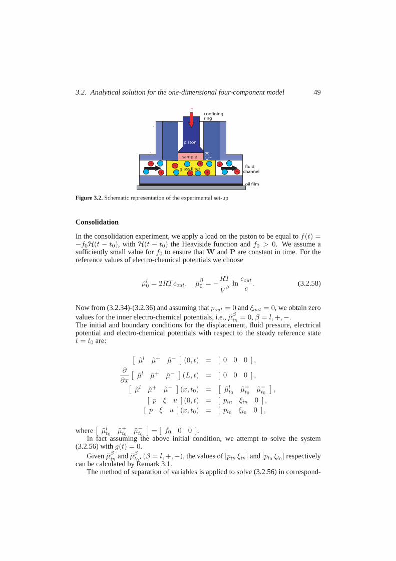
3.2. Analytical solution for the one-dimensional four-component model 49
piston
confiningring
sample
fluid channel
glass filter+
+
+
+
+
++++
++
F
L
oil film
Figure 3.2.Schematic representation of the experimental set-up
Consolidation
In the consolidation experiment, we apply a load on the piston to be equal tof(t) =−f0H(t − t0), with H(t − t0) the Heaviside function andf0 > 0. We assume asufficiently small value forf0 to ensure thatW andP are constant in time. For thereference values of electro-chemical potentials we choose
µl0 = 2RTcout, µβ
0 = −RT
Vβ
lncout
c. (3.2.58)
Now from (3.2.34)-(3.2.36) and assuming thatpout = 0 andξout = 0, we obtain zerovalues for the inner electro-chemical potentials, i.e.,µβ
in = 0, β = l,+,−.The initial and boundary conditions for the displacement, fluid pressure, electricalpotential and electro-chemical potentials with respect to the steady reference statet = t0 are:
[µl µ+ µ−
](0, t) = [ 0 0 0 ] ,
∂
∂x
[µl µ+ µ−
](L, t) = [ 0 0 0 ] ,
[µl µ+ µ−
](x, t0) =
[µl
t0 µ+t0
µ−t0],
[ p ξ u ] (0, t) = [ pin ξin 0 ] ,
[ p ξ u ] (x, t0) = [ pt0 ξt0 0 ] ,
where[µl
t0 µ+t0
µ−t0]
= [ f0 0 0 ].In fact assuming the above initial condition, we attempt to solve the system
(3.2.56) withg(t) = 0.Givenµβ
in andµβt0
, (β = l,+,−), the values of[pin ξin] and[pt0 ξt0 ] respectivelycan be calculated by Remark 3.1.
The method of separation of variables is applied to solve (3.2.56) in correspond-

50 Chapter 3. An analytical solution of incompressible charged porous media
ing with the boundary and initial conditions. The solutions are:
µl(x, t)µ+(x, t)µ−(x, t)
=
4
π
∞∑
n=0
1
2n+ 1sin
(2n+ 1
2
π
Lx
)M1RnM
−11
µlt0µ+
t0µ−t0
,
(3.2.59)in whichRn is a diagonal matrix with
Riin = exp
(−
(2n+ 1
2π
)2 λi(t− t0)
L2
), i = l,+,−. (3.2.60)
Using relation (3.2.49), (3.2.51) and (3.2.54) and after time integration we have
(pξ
)= H−1
ǫ FTE−1
µl(x, t)µ+(x, t)µ−(x, t)
− H−1
ǫ FTE−1f0H(t− t0)
(100
)
+ H−1ǫ f0
H(t− t0)
2µs + λs
(10
)+ f1(x).
By using the initial condition forp andξ at t = t+0 , the functionf1(x) is equal to
f1(x) =
(pt0ξt0
)−
(f0
0
).
Therefore we have
(pξ
)= H−1
ǫ FTE−1
µl(x, t) − µlt0
µ+(x, t) − µ+t0
µ−(x, t) − µ−t0
+
(pt0ξt0
).
By plugging equation (3.2.59) into the above identity we obtain
(p(x, t)ξ(x, t)
)= H−1
ǫ FTE−1 4
π
∞∑
n=0
1
2n+ 1×
sin
(2n+ 1
2
π
Lx
)M1(Rn − I)M−1
1
µlt0µ+
t0µ−t0
+
(pt0ξt0
). (3.2.61)
After integration in space of equations (3.2.45) we have
u(x, t) =1
2µs + λs
∫ x
0(p− pin) dx− f0H(t− t0)x+ f2(t).
3.2. Analytical solution for the one-dimensional four-component model 51
Assumingx = 0 and considering the boundary conditionu(0, t) = 0, we obtainf2(t) = 0. Let t = t+0 , then we have
pt0 = pin − f0.
Using the above fact and plugging (3.2.61) into the relation foru,
u(x, t) =1
2µs + λs( 1 0 )H−1
ǫ FTE−1 8L
π2
∞∑
n=0
1
(2n+ 1)2×
(1 − cos
(2n+ 1
2
π
Lx
))M1(Rn − I)M−1
1
µlt0µ+
t0µ−t0
. (3.2.62)
Given equations (3.2.25) and (3.2.59), the fluxesΦβxβs, β = l,+,− are equal to
ϕxls(x, t)ϕ+x+s(x, t)ϕ−x−s(x, t)
= −
2
L
∞∑
n=0
cos
(2n+ 1
2
π
Lx
)PM1RnM
−11
µlt0µ+
t0µ−t0
.
(3.2.63)
Free swelling
In the next experiment, we change the concentration of the external salt solution.Considering the reference values for the electro-chemical potentials to beequal tozero, the equations (3.2.41) and (3.2.42) yields the following boundary and initialconditions for the free swelling experiment:
[µl µ+ µ−
](0, t) =
[µl
in µ+in µ−in
],
∂
∂x
[µl µ+ µ−
](L, t) = [ 0 0 0 ] ,
[µl µ+ µ−
](x, t0) =
[µl
t0 µ+t0
µ−t0],
[ p ξ u ] (0, t) = [ pin ξin 0 ] ,
[ p ξ u ] (x, t0) = [ pt0 ξt0 0 ] ,
in which µβt0
= 0, β = l,+,−, and
µlin = −2RT∆cout,
µ+in =
RT
V+ ln
cout(t+0 )
cout(t−0 ),
µ−in =RT
V− ln
cout(t+0 )
cout(t−0 ),
(3.2.64)
∆cout is the change in the external concentration andt+0 andt−0 are the time just afterand beforet0 when chemical loading is applied.
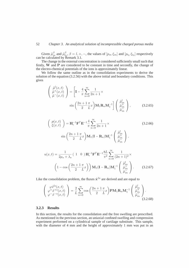
52 Chapter 3. An analytical solution of incompressible charged porous media
Given µβin andµβ
t0, β = l,+,−, the values of[pin ξin] and[pt0 ξt0 ] respectively
can be calculated by Remark 3.1.The change in the external concentration is considered sufficiently small such that
firstly, W andP are considered to be constant in time and secondly, the change ofthe electro-chemical potentials of the ions is approximately linear.
We follow the same outline as in the consolidation experiments to derive thesolution of the equation (3.2.56) with the above initial and boundary conditions. Thisgives
µl(x, t)µ+(x, t)µ−(x, t)
=
[I −
4
π
∞∑
n=0
1
2n+ 1×
sin
(2n+ 1
2
π
Lx
)M1RnM
−11
]
µlinµ+
inµ−in
, (3.2.65)
(p(x, t)ξ(x, t)
)= H−1
ǫ FTE−1 4
π
∞∑
n=0
1
2n+ 1× (3.2.66)
sin
(2n+ 1
2
π
Lx
)M1(I − Rn)M−1
1
µlinµ+
inµ−in
,
u(x, t) =1
2µs + λs( 1 0 )H−1
ǫ FTE−1 8L
π2
∞∑
n=0
1
(2n+ 1)2×
(1 − cos
(2n+ 1
2
π
Lx
))M1(I − Rn)M−1
1
µlinµ+
inµ−in
. (3.2.67)
Like the consolidation problem, the fluxesxβs are derived and are equal to
ϕxls(x, t)ϕ+x+s(x, t)ϕ−x−s(x, t)
=
2
L
∞∑
n=0
cos
(2n+ 1
2
π
Lx
)PM1RnM
−11
µlinµ+
inµ−in
.
(3.2.68)
3.2.3 Results
In this section, the results for the consolidation and the free swelling are prescribed.As mentioned in the previous section, an uniaxial confined swelling and compressionexperiment performed on a cylindrical sample of cartilage substitute. This sample,with the diameter of 4 mm and the height of approximately 1 mm was put in an

3.2. Analytical solution for the one-dimensional four-component model 53
insulating confining ring. A piston on the top of the sample was loaded mechanically.A bathing solution flowed through a porous glass filter at the bottom of the sample. Achange of the salt concentration of this solution generates a change in the boundaryof ion concentrations and electro-chemical potentials as well as pressureand voltage.
During the experiment, the mechanical and chemical load were varied. Inspiredby them, two numerical simulations are considered.
For both computations, the parameters in table 3.1 are considered:
Parameter Unit Value2µs + λs MPa 4 × 10³
K m4 N−1 s−1 1.0 × 10⁻¹⁸
cfc mol m−3 −2 × 10²
cout mol m−3 1 × 10²
ϕ 0.2D+ m2 s−1 13.3 × 10⁻¹⁰
D− m2 s−1 20.3 × 10⁻¹⁰
R J mol−1 K−1 8.3145T K 293F C mol−1 96484.6Γ 0.9ǫ C2 N−4 m−4 10−6
r 0.4
Table 3.1.Material parameters
Considering the above material parameters, the three eigenvalues in (3.2.56) are:
λ1 = 2.3324 × 10⁻¹ m2 s−1,
λ2 = 4.0 × 10⁻⁹ m2 s−1,
λ3 = 1.8 × 10⁻¹⁰ m2 s−1.
For the consolidation experiment, an inward force,f0 = 5 MPa is applied to theleft no-flow boundary, and at the right rigid boundary, the porous medium is in con-tact with an electro-neutral bathing solution. All boundary conditions are described.Note that in this experiment, all the unknowns change immediately att = t0 s,thus another equilibrium will be established in the end. At the final equilibrium, theelectro-chemical potentialsµβ , β = l,+,−, have the same value as the value in theinitial state. However, the stress and fluid pressure have changed, since the porousmedium is compressed. Figure 3.3 displays the solutions. As it can be seen thetimefor consolidation to occur is approximatelyt− t0 ≈ 0.16 h.
For the free swelling experiment, the initial and boundary conditions are chosen.In this experiment, we decrease the external salt concentration with a small amountfrom cout = 1 × 10² mol m−3 to cout = 0.995 × 10² mol m−3. Therefore, as on(3.2.42)µβ changes accordingly. The displacement, pore pressure, electrical poten-tial, electro-chemical potentials and ion concentrations are displayed in Figure 3.4.
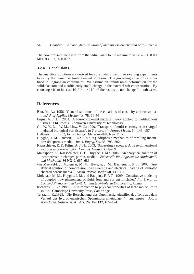
54 Chapter 3. An analytical solution of incompressible charged porous media
The pore pressure increases from the initial value to the maximum valuep = 0.0041MPa att− t0 ≈ 0.09 h.
3.2.4 Conclusions
The analytical solutions are derived for consolidation and free swelling experimentsto verify the numerical finite element solutions. The governing equations arede-fined in Lagrangian coordinates. We assume an infinitesimal deformation forthesolid skeleton and a sufficiently small change in the external salt concentration. Bychoosingǫ from interval10−5 ≤ ǫ ≤ 10−15 the results do not change for both cases.
References
Biot, M. A.: 1956, ‘General solutions of the equations of elasticity and consolida-tion.’ J. of Applied Mechanics.78, 91–96
Frijns, A. J. H.: 2001, ‘A four-component mixture theory applied to cartilaginoustissues.’ PhD-thesis, Eindhoven University of Technology.
Gu, W. Y., Lai, W. M., Mow, V. C.: 1999, ‘Transport of multi-electrolytes in chargedhydrated biological soft tissues’.in Transport in Porous Media.34, 143–157.
Helfferich, F.: 1962,Ion exchange.McGraw-Hill, New York.Huyghe, J. M., Janssen, J. D.: 1997, ‘Quadriphasic mechanics of swelling incom-
pressibleporous media.‘Int. J. Engng. Sci.35, 793–802.Kaasschieter, E. F., Frijns, A. J. H.: 2003, ‘Squeezing a sponge: A three-dimensional
solution in poroelasticity.’Comput. Geosci.7, 49–59.Malakpoor, K., Kaasschieter, E. F., Huyghe, J. M.: 2006, ‘An analytical solution of
incompressible charged porous media.’Zeitschrift fur Angewandte Mathematikund Mechanik.86 NO-9, 667–681
van Meerveld, J., Molenaar, M. M., Huyghe, J. M., Baaijens, F. P. T.: 2003, ‘An-alytical solution of compression, free swelling and electrical loading of saturatedcharged porous media.’Transp. Porous Media.50, 111–126.
Molenaar, M. M., Huyghe, J. M. and Baaijens, F. P. T.: 1999, ‘Constitutive modelingof coupled flow phenomena of fluid, ions and current in shales.’Int. Symp. onCoupled Phenomena in Civil, Mining& Petroleum Engineering, China.
Richards, E. G.: 1980, ‘An Introduction to physical properties of largemolecules insolute.’ Cambridge University Press, Cambridge.
Terzaghi, K.:1923, ‘Die Berechenung der Durchlassigheitsziffer desTons aus demVerlauf der hydrodynamischen Spanningserscheinungen.’Sitzungsber. AKad.Wien Math. Naturwiss, Kl. Abt. 2A.Vol.132, 105–124.
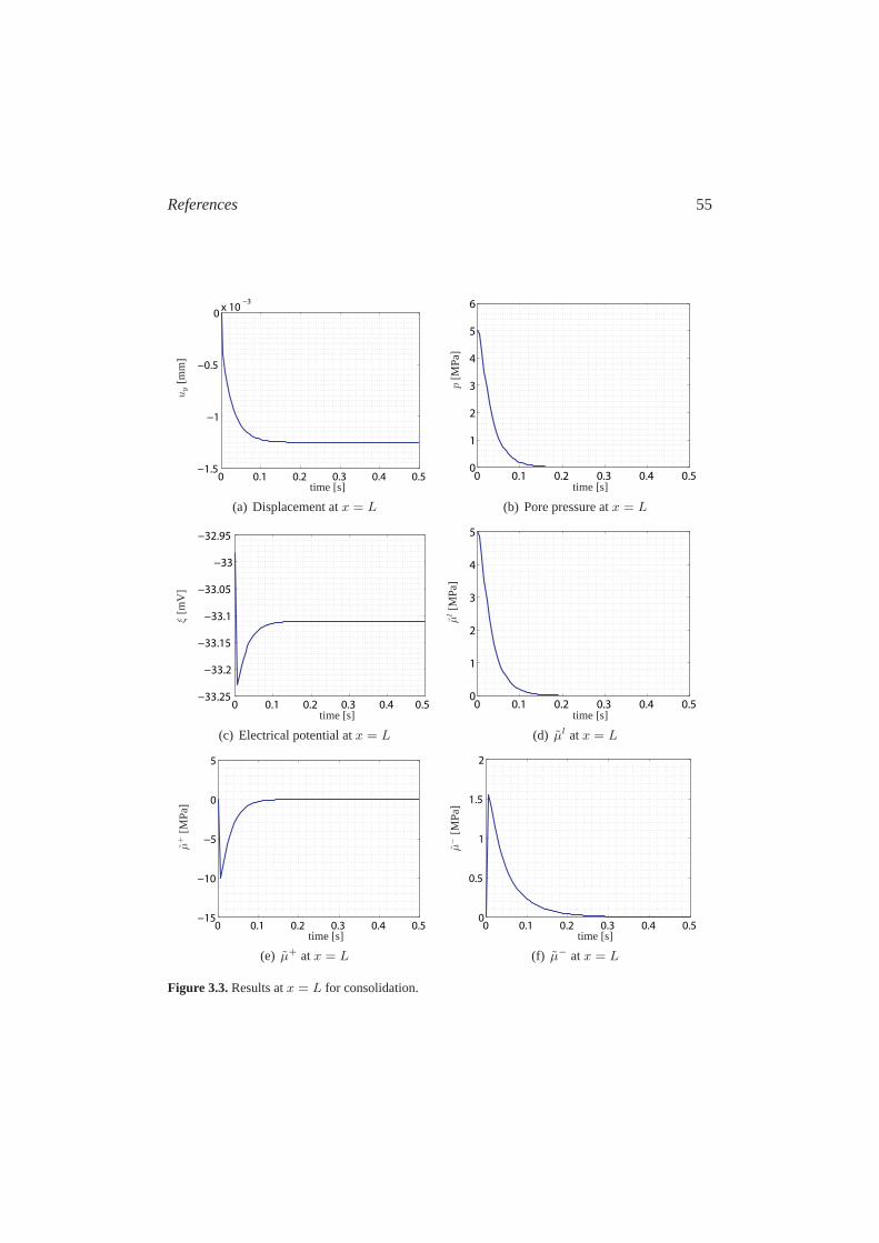
References 55
0 0.1 0.2 0.3 0.4 0.5−1.5
−1
−0.5
0x 10
−3
time [s]
uy
[mm
]
(a) Displacement atx = L
0 0.1 0.2 0.3 0.4 0.50
1
2
3
4
5
6
time [s]
p[M
Pa]
(b) Pore pressure atx = L
0 0.1 0.2 0.3 0.4−33.25
−33.2
−33.15
−33.1
−33.05
−33
−32.95
0.5time [s]
ξ[m
V]
(c) Electrical potential atx = L
0 0.1 0.2 0.3 0.4 0.50
1
2
3
4
5
time [s]
µl[M
Pa]
(d) µl atx = L
0 0.1 0.2 0.3 0.4 0.5−15
−10
−5
0
5
time [s]
µ+
[MP
a]
(e) µ+ atx = L
0 0.1 0.2 0.3 0.4 0.50
0.5
1
1.5
2
time [s]
µ−
[MP
a]
(f) µ− atx = L
Figure 3.3.Results atx = L for consolidation.
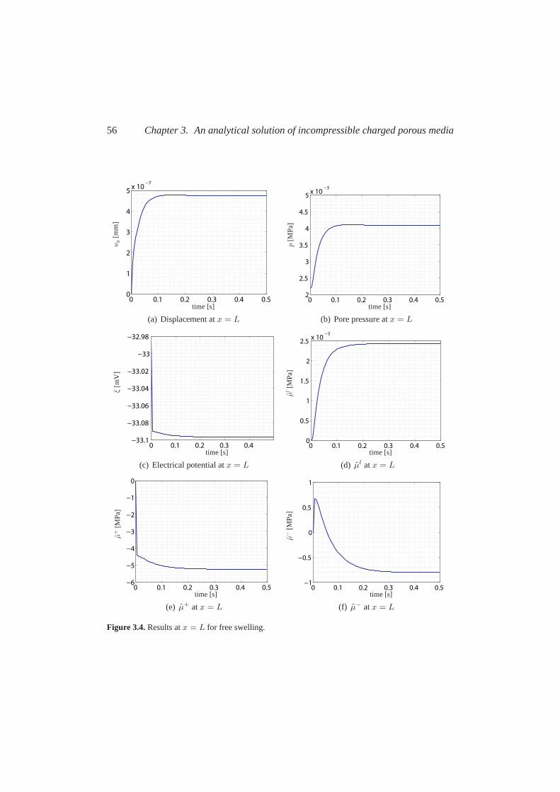
56 Chapter 3. An analytical solution of incompressible charged porous media
0 0.1 0.2 0.3 0.4 0.50
1
2
3
4
5x 10
−7
time [s]
uy
[mm
]
(a) Displacement atx = L
0 0.1 0.2 0.3 0.4 0.52
2.5
3
3.5
4
4.5
5x 10
−3
time [s]
p[M
Pa]
(b) Pore pressure atx = L
0 0.1 0.2 0.3 0.4−33.1
−33.08
−33.06
−33.04
−33.02
−33
−32.98
time [s]
ξ[m
V]
(c) Electrical potential atx = L
0 0.1 0.2 0.3 0.4 0.50
0.5
1
1.5
2
2.5x 10
−3
time [s]
µl[M
Pa]
(d) µl atx = L
0 0.1 0.2 0.3 0.4 0.5−6
−5
−4
−3
−2
−1
0
time [s]
µ+
[MP
a]
(e) µ+ atx = L
0 0.1 0.2 0.3 0.4 0.5−1
−0.5
0
0.5
1
time [s]
µ−
[MP
a]
(f) µ− atx = L
Figure 3.4.Results atx = L for free swelling.

Chapter 4
Mixed and hybrid finite element solution fortwo-components
While searching for a quantitative description of physical phenomena, the en-gineer or physicist establishes generally a system of ordinary or partialdif-
ferential equations valid in a certain region (or domain) and imposes on this systemsuitable boundary and initial conditions. At this stage the mathematical model iscomplete, and for practical applications “merely” a solution for a particular set of nu-merical data is needed. Here, however, come the major difficulties, as only the verysimplest forms of equations, within geometrically trivial boundaries, are capable ofbeing solved exactly with available mathematical methods.
To enlist the aid of the most powerful tool developed in this century - the digitalcomputer - it is necessary to recast the problem in a purely algebraic form,involvingonly the basic arithmetic operations. To achieve this, various forms of discretisationof the continuum problem defined by differential equations can be used.In such a dis-cretisation the infinite set of numbers representing the unknown function orfunctionsis replaced by a finite number of unknown parameters, and this process, ingeneral,requires some form of approximation.
Of the various forms of discretisation that are possible, one of the most used isthe finite difference process. Another method that is often used in many physicalapplications is concerned with various trial function approximations falling underthe general classification of finite element methods. It has been shown thatevenfinite difference processes can be included as a subclass of this more general theory(Ciarlet, 1978).
The name “mixed method” is applied to a variety of finite element methods thathave more than one approximation space. Typically one or more of the spaces playthe role of Lagrange multipliers to enforce constraints. The name and many ofthe original concepts for such methods originated in solid mechanics where itwasdesirable to have a more accurate approximation of certain derivatives ofdisplace-ment. However, for the Stokes equations that govern viscous fluid flow, the naturalGalerkin approximation is a mixed method (Babuska, 1973), (Babuska and Aziz,1973), (Brezzi, 1974), (Fortin, 1977) and (Brezzi and Fortin, 1991).
57
58 Chapter 4. Mixed and hybrid finite element solution for two-components
As it was mentioned, in a mixed formulation the gradient of the solution is in-troduced as a separate dependent variable of which the approximation is sought in adifferent finite element space than the solution itself.
The main advantage of this method is that it suffices to use finite elements of classC0 whereas finite elements of classC1 would be required for conforming methods.Another advantage (from the point of view of fluid mechanics and in particular ourtwo- and four-component mixture model) is that the present method not only yieldsa continuous approximation of the solution, but also of the derivatives of the solution(which, in addition need to be computed).
The mixed finite element method has been extensively used for the solutionof parabolic equations arising in different application fields. The mixed finiteele-ment method was proposed for two-dimensional problems by (Raviart and Thomas,1977), (Thomas, 1977) and (Roberts and Thomas, 1991), and by Nedelec for three-dimensional problems (Nedelec, 1980) and (Nedelec, 1986).
Cartilaginous tissues are soft hydrated tissues with strong swelling and shrinkageproperties. This swelling and shrinkage behaviour of cartilaginous tissues is causedby the flow of water that is bound to the charged, solid skeleton of the porous tissue.The driving mechanism is an interplay of mechanical, chemical and electricalforces.In chapter 2 a finite deformation four-component model has been derived to accountfor osmotic effects. To account for finite deformation the set of equationsis written inLagrangian coordinates. This leads to a system of coupled time dependentnon-linearequations together with boundary conditions.
In our model it is desirable to obtain approximations of the fluid flow and ionsflow that fulfil the conservation equations. In finite element simulations (van Loonet al., 2003), these quantities are generally calculated by differentiation ofthe electro-chemical potential solutions. This approach may lead to violation of the mass con-servation principle.
The mixed finite element method provides an attractive framework for this typeof problems by simultaneously approximating flows and electro chemical potentials.Flows computed by mixed finite elements automatically satisfy the “divergence free”property, both locally and globally, and the corresponding normal flux field is guaran-teed to be continuous across inter-element boundaries. In this chapter themixed finiteelement variational formulation is derived for the set of coupled equationsdescrib-ing the two-component model in general dimensions. Only the lowest-order mixedmethod will be considered, first, because higher order-methods result insome con-ceptual complications and, second, because the lowest-order method is comparativelyeasy and straightforward to use for practical problems.
It is more useful to propose the mixed method first for the linear two-componentmodel (2.8.1). In fact this will give a basis from which to continue the mixed methodfor the four-component model.
This chapter is outlined as follows. In the first section preliminary definitions offunction spaces are given. In section 2 we propose a mixed formulation for the two-component mixture. In this section the existence and uniqueness for the discretisedsystem is proven. In section 3 we introduce the mixed hybrid technique. Section 4 isdevoted to numerical results for given examples.

4.1. Notations and Preliminaries 59
4.1 Notations and Preliminaries
In this section we will introduce some notations and definitions crucial for the mixedformulation (Ciarlet, 1978).
Throughout this article,Ω shall denote a bounded, open, connected subset ofRn,
n = 1, 2, 3, with a Lipschitz continuous boundaryΓ (Ciarlet, 1978, p. 12).Define ΩT = Ω × (0, T ] for T > 0 and consider the setsΓD
u and ΓNu (and
similarly ΓDp andΓN
p ) to be two disjoint open subsets of the total boundaryΓ = ∂Ω,such that
ΓDα ∩ ΓN
α = ∅ and ΓDα ∪ ΓN
α = Γ for α = u, p.
We assumemeasΓD
α > 0 for α = u, p.
L2(Ω) is the set of all Lebesgue measurable scalar functionsf : Ω → R such that
‖f‖0 =
(∫
Ωf2dx
)1/2
<∞.
L2(Ω) is the set of all Lebesgue measurable vector functionsf : Ω → Rn such that
‖f‖0 =
(∫
Ω|f |2dx
)1/2
<∞.
Let k be a nonnegative integer, thenHk(Ω) denotes the Sobolev space,
Hk(Ω) =v ∈ L2(Ω) : Dαv ∈ L2(Ω) for all |α| ≤ k
,
equipped with the norm‖v‖k =
∑
|α|≤k
‖Dαv‖0.
In the above definition
Dαv =∂|α|v
∂xα11 · · · ∂xαn
n, α = (α1, · · · , αn) ∈ N
n with |α| =n∑
i=1
αi,
where differentiation is to be understood in the weak sense.Let C∞
0 (Ω) denote the space of all infinitely differentiable scalar functionsϕ :Ω → R with compact support inΩ. We denote byHk
0 (Ω) the closure of the spaceC∞
0 (Ω) in Hk(Ω). Moreover if we define
|v|k =∑
|α|=k
‖Dαv‖0.
Note that| · |1 and‖ · ‖1 are equivalent norms inH10 (Ω).
60 Chapter 4. Mixed and hybrid finite element solution for two-components
We denote byH−k(Ω) the dual space toHk0 (Ω). Forf ∈ H−k(Ω),
‖f‖−k = sup06=v∈Hk
0 (Ω)
(f, v)
‖v‖k
defines the related norm, where(·, ·) denotes the duality pairing betweenH−k(Ω)andHk
0 (Ω).Let k = 1, for ϕ ∈ H1(Ω), the traceγDϕ = ϕ|Γ is well-defined and is inL2(Γ).
In other words there exists a constantC, depending only onΩ, such that
‖ϕ‖0,Γ ≤ C‖ϕ‖1 for all ϕ ∈ H1(Ω).
The image of the above trace mapping is denoted by
H1/2(Γ) =γDϕ : ϕ ∈ H1(Ω)
,
and is a Hilbert space with norm
‖ψ‖1/2 = infϕ∈H1(Ω)
‖ϕ‖1 : ψ = γDϕ .
Define the functional space
H(div; Ω) = q ∈ L2(Ω) : ∇ · q ∈ L2(Ω),
and the inner product
(q1,q2)div;Ω =
∫
Ω(q1 · q2 + ∇ · q1∇ · q2) dx for all q1,q2 ∈ H(div; Ω).
The spaceH(div; Ω) with this inner product is a Hilbert space. The norm inH(div; Ω)will be defined as
‖q‖div;Ω = (q,q)1/2div;Ω.
If q ∈ H(div; Ω), then the traceγNq = n · q, wheren is the outward normal toΓ,is well defined (Brezzi and Fortin, 1991, Lemma III.1.1) and we denote
H−1/2(Γ) = γNq : q ∈ H(div; Ω)
with norm
‖µ‖−1/2,Γ = infq∈H(div;Ω)
‖q‖H(div;Ω) : µ = γNq for all µ ∈ H−1/2(Γ).
We shall use the following version of Green’s formula:∫
Ω(ϕ∇ · q + ∇ϕ · q) dx =
∫
Γϕq · n ds,
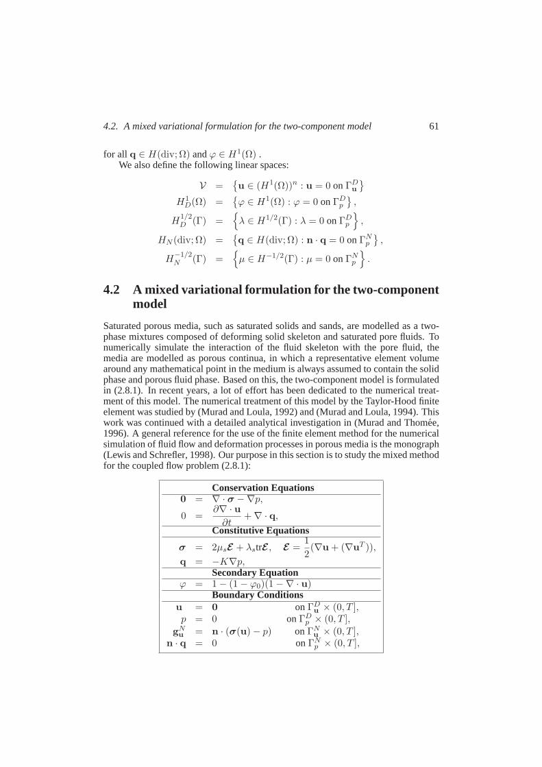
4.2. A mixed variational formulation for the two-component model 61
for all q ∈ H(div; Ω) andϕ ∈ H1(Ω) .We also define the following linear spaces:
V =u ∈ (H1(Ω))n : u = 0 onΓD
u
H1D(Ω) =
ϕ ∈ H1(Ω) : ϕ = 0 onΓD
p
,
H1/2D (Γ) =
λ ∈ H1/2(Γ) : λ = 0 onΓD
p
,
HN (div; Ω) =q ∈ H(div; Ω) : n · q = 0 onΓN
p
,
H−1/2N (Γ) =
µ ∈ H−1/2(Γ) : µ = 0 onΓN
p
.
4.2 A mixed variational formulation for the two-componentmodel
Saturated porous media, such as saturated solids and sands, are modelledas a two-phase mixtures composed of deforming solid skeleton and saturated pore fluids. Tonumerically simulate the interaction of the fluid skeleton with the pore fluid, themedia are modelled as porous continua, in which a representative element volumearound any mathematical point in the medium is always assumed to contain the solidphase and porous fluid phase. Based on this, the two-component model isformulatedin (2.8.1). In recent years, a lot of effort has been dedicated to the numerical treat-ment of this model. The numerical treatment of this model by the Taylor-Hood finiteelement was studied by (Murad and Loula, 1992) and (Murad and Loula,1994). Thiswork was continued with a detailed analytical investigation in (Murad and Thomee,1996). A general reference for the use of the finite element method for the numericalsimulation of fluid flow and deformation processes in porous media is the monograph(Lewis and Schrefler, 1998). Our purpose in this section is to study the mixed methodfor the coupled flow problem (2.8.1):
Conservation Equations0 = ∇ · σ −∇p,
0 =∂∇ · u
∂t+ ∇ · q,
Constitutive Equations
σ = 2µsE + λstrE , E =1
2(∇u + (∇uT )),
q = −K∇p,Secondary Equation
ϕ = 1 − (1 − ϕ0)(1 −∇ · u)Boundary Conditions
u = 0 onΓDu × (0, T ],
p = 0 onΓDp × (0, T ],
gNu = n · (σ(u) − p) onΓN
u × (0, T ],n · q = 0 onΓN
p × (0, T ],

62 Chapter 4. Mixed and hybrid finite element solution for two-components
where, we omitted the superscriptl from ql in (2.8.1).
4.2.1 Variational formulation
For the preliminary step of defining a spatially semi-discrete approximate solutiontoour initial boundary value problem, we write the problem in weak form. Consideringthe flux q and the flux spaceHN (div; Ω), the above system of equations can beformally written as a first- order system whose mixed variational formulation givesrise to the following system of variational equations:Find (u,q, p) (·, t) ∈ V ×HN (div; Ω) × L2(Ω), such that
∫
Ω(2µsE(u) : E(u) + λs∇ · u∇ · u) dx −
∫
Ωp∇ · u dx =
∫
ΓNu
gNu · u ds,
(4.2.1a)1
K
∫
Ωq · q dx −
∫
Ωp∇ · q dx = 0, (4.2.1b)
−
∫
Ω∇ · qp dx −
∫
Ω
∂∇ · u
∂tp dx = 0, (4.2.1c)
for all test functions(u, q, p) ∈ V ×HN (div; Ω) × L2(Ω) andt > 0. Note that thesolution is time-dependent.
Define
a(u, u) =
∫
Ω(2µsE(u) : E(u) + λs∇ · u∇ · u) dx,
b(u, p) = −
∫
Ω∇ · up dx,
c(q, q) =1
K
∫
Ωq · q dx,
d(q, p) = −
∫
Ω∇ · qp dx,
f(u) =
∫
ΓNu
gNu · u ds,
then the problem (4.2.1a)-(4.2.1c) can be rewritten as follows:
Find (u,q, p) ∈ V ×HN (div; Ω) × L2(Ω) such that
a(u, u) +b(u, p) =f(u),c(q, q) +d(q, p) = 0,
d
dtb(u, p)+d(q, p) = 0,
(4.2.2)
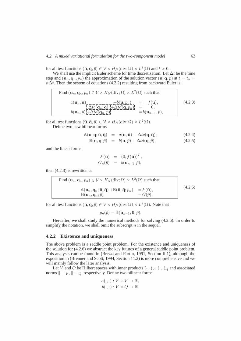
4.2. A mixed variational formulation for the two-component model 63
for all test functions(u, q, p) ∈ V ×HN (div; Ω) × L2(Ω) andt > 0.We shall use the implicit Euler scheme for time discretisation. Let∆t be the time
step and(un,qn, pn) the approximation of the solution vector(u,q, p) at t = tn =n∆t. Then the system of equations (4.2.2) resulting from backward Euler is:
Find (un,qn, pn) ∈ V ×HN (div; Ω) × L2(Ω) such that
a(un, u) +b(u, pn) = f(u),∆tc(qn, q) +∆td(q, pn) = 0,
b(un, p) +∆td(qn, p) =b(un−1, p),
(4.2.3)
for all test functions(u, q, p) ∈ V ×HN (div; Ω) × L2(Ω).Define two new bilinear forms
A(u,q; u, q) = a(u, u) + ∆tc(q, q), (4.2.4)B(u,q; p) = b(u, p) + ∆td(q, p), (4.2.5)
and the linear forms
F (u) = (0, f(u))T ,
Gn(p) = b(un−1, p),
then (4.2.3) is rewritten as
Find (un,qn, pn) ∈ V ×HN (div; Ω) × L2(Ω) such that
A(un,qn; u, q) +B(u, q; pn) =F (u),B(un,qn; p) =G(p),
(4.2.6)
for all test functions(u, q, p) ∈ V ×HN (div; Ω) × L2(Ω). Note that
gn(p) = B(un−1,0; p).
Hereafter, we shall study the numerical methods for solving (4.2.6). In order tosimplify the notation, we shall omit the subscriptn in the sequel.
4.2.2 Existence and uniqueness
The above problem is a saddle point problem. For the existence and uniqueness ofthe solution for (4.2.6) we abstract the key futures of a general saddle point problem.This analysis can be found in (Brezzi and Fortin, 1991, Section II.1), although theexposition in (Brenner and Scott, 1994, Section 11.2) is more comprehensive and wewill mainly follow the later analysis.
Let V andQ be Hilbert spaces with inner products(·, ·)V , (·, ·)Q and associatednorms‖ · ‖V , ‖ · ‖Q, respectively. Define two bilinear forms
a(·, ·) : V × V → R,
b(·, ·) : V ×Q→ R.
64 Chapter 4. Mixed and hybrid finite element solution for two-components
It is natural to assume that these forms are continuous:
a(u, v) ≤ ‖a‖‖u‖V ‖v‖V for all u, v ∈ V,
b(u, p) ≤ ‖b‖‖u‖V ‖p‖Q for all u ∈ V, p ∈ Q.
We denote byV ∗ andQ∗ the dual spaces ofV andQ, respectively and further sup-pose that bounded linear functionalsf ∈ V ∗ andg ∈ Q∗ are given. We investigatethe existence and uniqueness of a solution of the saddle point problem:
Find (u, p) ∈ V ×Q such that
a(u, v) +b(v, p) =(f, v)V ∗,V , v ∈ V,b(u, q) =(g, q)Q∗,Q , q ∈ Q.
(4.2.7)
Denote byA : V → V ∗ andB : V → Q∗ the bounded linear operators associatedwith the bilinear formsa(·, ·) andb(·, ·) according to
(Au, v)V ∗,V = a(u, v), u, v ∈ V,
(Bv, q)Q∗,Q = b(v, q), v ∈ V, q ∈ Q,
and
F (v) = (f, v)V ∗,V ,
G(q) = (g, q)Q∗,Q,
then the saddle point (4.2.7) can be equivalently written as the following system ofoperator equations
Au + B∗p = F in V ∗,Bu = G in Q∗.
, (4.2.8)
The kernels of the operatorB andB∗ are defined by
ker(B) = u ∈ V | b(u, q) = 0 for all q ∈ Q,
ker(B∗) = q ∈ Q | b(u, q) = 0 for all u ∈ V ,
Theorem 4.1(Existence and uniqueness result). LetV andQ be Hilbert spaces andlet a(·, ·) : V × V → R and b(·, ·) : V × Q → R be bounded bilinear forms withassociated operatorsA : V → V ∗ andB : V → Q∗ such that there holds:
(i) The bilinear forma(·, ·) is ker(B)-elliptic, i.e., there exists a constantα > 0such that
a(v0, v0) ≥ α‖v0‖2V , v0 ∈ ker(B).
(ii) The bilinearb(·, ·) satisfies the inf-sup condition
infq∈Q\ker(B∗)
supv∈V
b(v, q)
‖v‖V ‖q‖Q\ker(B∗)≥ β.

4.2. A mixed variational formulation for the two-component model 65
Then for anyf ∈ V ∗ and g ∈ Im(B), the saddle point problem(4.2.7)admits asolution(u, p) ∈ V ×Q, whereu ∈ V is uniquely determined andp ∈ Q is uniqueup to an element ofker(B∗). Moreover one has the bounds
‖u‖V ≤1
α‖f‖V ∗ +
(1 +
‖a‖
α
)1
β‖g‖Q∗ , (4.2.9)
‖p‖Q\ker(B∗) ≤1
β
(1 +
‖a‖
α
)‖f‖V ∗ +
‖a‖
β2
(1 +
‖a‖
α
)‖g‖Q∗ . (4.2.10)
Proof. See for example (Brezzi and Fortin, 1991, Chapter 2).
Now we return to the saddle point problem (4.2.6). We equip the spaceV ×HN (div; Ω) with a norm
9 (u,q)91 =(‖u‖2
1 + ‖q‖2div;Ω
)1/2. (4.2.11)
To prove theker(B)-ellipticity of A, we need the following lemma.
Lemma 4.2 (Korn’s second inequality). Let Ω ⊂ R3 be an open bounded set with
smooth boundary. In addition, suppose thatΓ0 ⊂ ∂Ω has positive two-dimensionalmeasure. Then there exists a positive numberc(Ω,Γ0) such that
∫
ΩE(u) : E(u) dx ≥ c(Ω,Γ0)‖u‖
21 for all u ∈ V. (4.2.12)
Proof. See for example (Brezzi and Fortin, 1991).
Using Korn’s inequality, we show that the bilinear formA is ker(B)-elliptic onV ×HN (div; Ω). The definition of the subspaceker(B) implies that
∇ · u + ∆t∇ · q = 0 for all (u,q) ∈ ker(B). (4.2.13)
Using Korn’s inequality, we get
A((u,q), (u,q)) = a(u, u) + ∆tc(q, q)
≥ 2µsc‖u‖21 + λs‖∇ · u‖2
0 +K−1∆t‖q‖20
= 2µsc‖u‖21 + λs(∆t)
2‖∇ · q‖20 +K−1∆t‖q‖2
0
≥ α(‖u‖2
1 + ‖q‖2div;Ω
)
= α 9 (u,q)921,
(4.2.14)
for all (u,q) ∈ ker(B) and whereα = min(2µsc, λs(∆t)2,K−1∆t).
The second condition in Theorem 4.1 is inf-sup condition:
sup(u,q)∈V×HN (div;Ω)
B(q, (u,q))
9(u,q)91≥ β‖q‖, for all q ∈ L2(Ω), (4.2.15)

66 Chapter 4. Mixed and hybrid finite element solution for two-components
where we assume implicitly that the left side has to be evaluated only for‖(u,q)‖1 6=0. We restrict the supremum to a subset of functions(0,q), therefore we obtain alower estimate forβ:
∆t supq∈HN (div;Ω)
d(q,q)
‖q‖div;Ω≥ β‖q‖0, for all q ∈ L2(Ω). (4.2.16)
We need the following lemma to prove this inequality:
Lemma 4.3. There exists a positive constantC such that for allq ∈ L2(Ω) thereexists a functionq ∈ HN (div; Ω) satisfying
−∇ · q = q
and‖q‖div;Ω ≤ C‖q‖0.
Proof. Let q ∈ L2(Ω), then by the Lax-Miligram Theorem (Brenner and Scott, 1994,Theorem 2.7.7) there exists a uniqueΦ ∈ H1
D(Ω) satisfying−∆Φ = q in Ω,
∇Φ · n = 0 onΓNp .
If we defineq = ∇Φ, thenq ∈ HN (div; Ω) and we have∫
Ωq∇Φdx =
∫
ΩqΦdx for all Φ ∈ H1
D(Ω).
By choosingΦ = Φ, we have
‖q‖20 =
∫
ΩqΦ dx ≤ ‖q‖0‖Φ‖0 ≤ C(Ω)‖q‖0‖∇Φ‖0,
where the last inequality was derived by the Poincare inequality (Brenner and Scott,1994, Proposition 5.3.5).
Let q ∈ L2(Ω), then by above the lemma there exists a functionq ∈ HN (div; Ω)such that−∇ · q = q and
‖q‖div;Ω ≤ C‖q‖0
for some constantC. Use the fact that
d(q, q) = −
∫
Ω∇ · qq dx =
∫
Ωq2 dx = ‖q‖2
0,
thus
∆t supq∈HN (div;Ω)
d(q,q)
‖q‖div;Ω≥ ∆t
d(q, q)
‖q‖div;Ω≥
∆t
C‖q‖0.
Therefore the inf-sup condition holds for allβ ≤∆t
C. The following result follows
immediately from Theorem 4.1.
4.2. A mixed variational formulation for the two-component model 67
Theorem 4.4. The saddle point problem(4.2.6):
Find (u,q, p) ∈ V ×HN (div; Ω) × L2(Ω) such that
A(u,q; u, q) +B(u, q; p) =F (u),B(u,q; p) =G(p),
has a unique solution. moreover one has the bounds
9 (un,qn)91 ≤1
α‖F‖−1 +
(1 +
‖A‖
α
)1
β‖B‖‖un−1‖1, (4.2.17)
‖pn‖L2(Ω)\ker(B∗) ≤1
β
(1 +
‖A‖
α
)‖F‖−1 +
‖A‖
β2
(1 +
‖A‖
α
)‖B‖‖un−1‖1.
(4.2.18)
4.2.3 Mixed finite element approximation
Assume thatΩ is a polygon (n=2) or a polyhedron (n=3). We denote byTh a tri-angulation ofΩ by n-simplicesT of diameter not greater thanh (T is a triangle orrectangle forn = 2, a tetrahedron or block forn = 3), where
Ω =⋃
T∈Th
T.
For the definition of a triangulation, see (Ciarlet, 1978, page 38), for example. Weshall also use the notation:
- measT = the Euclidian measure ofT in Rn (geometric area ifn = 2, geo-
metric volume ifn = 3),
- hT = the diameter ofT , which in case of a triangulation by simplices, is justthe length of the longest edge,
- ρT = the radius of the circle inscribed inT if n = 2, or of the sphere inscribedin T if n = 3,
- h = maxT∈Th
hT .
A family of triangulationsTh : h > 0 is said to be regular if
infh>0
h = 0, infh>0
minT∈Th
ρT
hT> 0.
Now in order to state a finite element formulation of problem (4.2.6), it is necessaryto define finite-dimensional subspaces ofV,HN (div; Ω) andL2(Ω).
68 Chapter 4. Mixed and hybrid finite element solution for two-components
LetH(div; Th) be the space of square-integrable vectorial functionsq ∈ L2(Ω),whose divergences are square -integrable on every sub-domainT ∈ Th, i.e.
H(div; Th) = q ∈ L2(Ω) : q|T ∈ H(div;T ) for all T ∈ Th, (4.2.19)
with norm
‖q‖div;Th=
‖q‖2
0 +∑
T∈Th
‖∇ · q|T ‖20
1/2
. (4.2.20)
The following lemma gives a characterization of the functions inHN (div; Ω).
Lemma 4.5. A functionq ∈ H(div; Th) is inHN (div; Ω), if and only if
∑
T∈Th
∫
∂TΦnT · q ds = 0 for all Φ ∈ H1
D(Ω).
Proof. (⇒) Let q ∈ H(div; Th) and suppose that the above inequality holds. Definef ∈ L2(Ω) by
f |T = ∇ · q|T for all T ∈ Th,
then∫
ΩfΦ dx =
∑
T∈Th
∫
T∇ · q|T Φ dx
=∑
T∈Th
∫
∂TΦnT · q ds−
∑
T∈Th
∫
Tq · ∇Φ dx
= −∑
T∈Th
∫
∂Tq · ∇Φ dx
= −
∫
Ωq · ∇Φ dx for all Φ ∈ C∞
0 (Ω).
Thereforef = ∇ · q and thusq ∈ H(div; Ω). Finally Green’s formula implies∫
ΓΦn · q ds =
∑
T∈Th
∫
∂TΦnT · q ds = 0 for all Φ ∈ H1
D(Ω),
thusn · q = 0 onΓpN . Thereforeq ∈ HN (div; Ω).
(⇐) Let q ∈ HN (div; Ω), thenq ∈ HN (div; Th) and
∑
TTh
∫
∂TΦnT · q ds =
∫
ΓΦn · q ds = 0 for all Φ ∈ H1
D(Ω).
4.2. A mixed variational formulation for the two-component model 69
The following lemma gives an abstract view for the approximation of the problem(4.2.6). It provides the conditions for the existence and uniqueness of the approxi-mated solution.
Lemma 4.6. LetVh ⊂ V,Wh ⊂ HN (div; Ω) andQh ⊂ L2(Ω) be finite dimensionalsubspaces. Denote by
Ah : Vh ×Wh → Vh ×Wh,
Bh : Vh ×Wh → Qh,
the bounded linear operators associated with the bilinear formA andB restricted tothe finite dimensional subspacesVh ×Wh andQh. Consider the following problem:
Find (uh,qh, ph) ∈ Vh ×Wh ×Qh such that
A(uh,qh; uh, qh) +B(uh, qh; ph) =f(uh),B(uh,qh; ph) = g(ph),
for all test functions(uh, qh, ph) ∈ Vh ×Wh ×Qh.In the same way as for the continuous problem, we define a closed subspace ofVh ×Wh:
ker(Bh) = (uh,qh) ∈ Vh ×Wh : B(uh,qh; qh) = 0 for all qh ∈ Qh.
If div Vh + div Wh = Qh, then
1. ker(Bh) ⊂ ker(B),
2. A is ker(Bh)-elliptic, i.e., there exists anα > 0 such that
Ah(uh,qh;uh,qh) ≥ α 9 (uh,qh) 921 for all (uh,qh) ∈ ker(Bh),
3. B satisfies the LBB condition, i.e., there exists aβ > 0 such that
sup(uh,qh)∈Vh×Wh
B(uh,qh; qh)
9(uh,qh)91≥ β‖qh‖ for all qh ∈ Qh,
Proof. See (Brezzi and Fortin, 1991, p.138)
Existence and uniqueness of the solution(uh,qh, ph) ∈ Vh ×Wh ×Qh follows,as in the continuous problem, directly from Theorem 4.1. Additionally, we canderiveerror estimates in the terms of approximation properties of the spacesVh,Wh andQh.
Theorem 4.7. If div Vh + div Wh = Qh, then the mentioned saddle point problemin the above lemma has a unique solution(uh,qh, ph) ∈ Vh ×Wh ×Qh. Moreover,
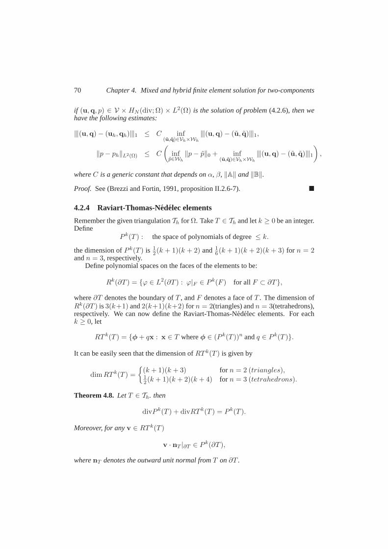
70 Chapter 4. Mixed and hybrid finite element solution for two-components
if (u,q, p) ∈ V × HN (div; Ω) × L2(Ω) is the solution of problem(4.2.6), then wehave the following estimates:
9(u,q) − (uh,qh)91 ≤ C inf(u,q)∈Vh×Wh
9(u,q) − (u, q)91,
‖p− ph‖L2(Ω) ≤ C
(inf
p∈Wh
‖p− p‖0 + inf(u,q)∈Vh×Wh
9(u,q) − (u, q)91
),
whereC is a generic constant that depends onα, β, ‖A‖ and‖B‖.
Proof. See (Brezzi and Fortin, 1991, proposition II.2.6-7).
4.2.4 Raviart-Thomas-Nedelec elements
Remember the given triangulationTh for Ω. TakeT ∈ Th and letk ≥ 0 be an integer.Define
P k(T ) : the space of polynomials of degree≤ k.
the dimension ofP k(T ) is 12(k + 1)(k + 2) and 1
6(k + 1)(k + 2)(k + 3) for n = 2andn = 3, respectively.
Define polynomial spaces on the faces of the elements to be:
Rk(∂T ) = ϕ ∈ L2(∂T ) : ϕ|F ∈ P k(F ) for all F ⊂ ∂T,
where∂T denotes the boundary ofT , andF denotes a face ofT . The dimension ofRk(∂T ) is 3(k+1) and2(k+1)(k+2) for n = 2(triangles) andn = 3(tetrahedrons),respectively. We can now define the Raviart-Thomas-Nedelec elements. For eachk ≥ 0, let
RT k(T ) = φ + qx : x ∈ T whereφ ∈ (P k(T ))n andq ∈ P k(T ).
It can be easily seen that the dimension ofRT k(T ) is given by
dimRT k(T ) =
(k + 1)(k + 3) for n = 2 (triangles),12(k + 1)(k + 2)(k + 4) for n = 3 (tetrahedrons).
Theorem 4.8. LetT ∈ Th. then
divP k(T ) + divRT k(T ) = P k(T ).
Moreover, for anyv ∈ RT k(T )
v · nT |∂T ∈ P k(∂T ),
wherenT denotes the outward unit normal fromT on∂T .
4.2. A mixed variational formulation for the two-component model 71
Proof. LetT ∈ Th. The first statement is trivial from the definition of the polynomialand Raviart-Thomas-Nedelec spaces. Letv ∈ RT k(T ) andx ∈ ∂T , then
(v · nT )(x) = φ(x) · nT (x) + q(x)x · nT (x),
whereφ ∈ (P k(T ))n andq ∈ P k(∂T ). Now x · nT (x) is constant on each faceF ∈ ∂T , and thereforev · nT |∂T ∈ P k(∂T ).
To uniquely define a function inRT k(T ) we have:
Theorem 4.9. LetT ∈ Th andv ∈ RT k(T ). If∫
∂Tv · nT p ds = 0 for all ϕ ∈ P k(∂T ),
∫
Tv · ϕ dx ds = 0 for all ϕ ∈ (P k−1(T ))n,
thenv = 0.
Proof. See (Brezzi and Fortin, 1991, proposition III.3.3).
Theorems 4.8 and 4.9 imply that we can use the following degrees of freedomtouniquely define a functionv ∈ RT k(T ) (see Figure 4.1):
• The moments of order up tok of v · nT on each faceF of T , i.e.∫
Fv · nTϕ ds ϕ ∈ P k(∂T ).
• The momentum of order up tok − 1 of v onT , for k > 0, i.e.∫
Tv · ϕ dx ϕ ∈ (P k−1(∂T ))n.
4.2.5 The lowest order Raviart-Thomas element
The most interesting case from the computational point of view is the lowest orderRaviart-Thomas element, i.e.,k = 0, especially when we can not expect hight regu-larity of the solutions of the continuous problem. We start with defining a local basisfunction ofRT 0 on a reference element.
Let T be the convex hull ofL suitably chosen pointsxℓ, ℓ = 1, . . . , L, that is
T =
x =
L∑
1
ζℓxℓ : 0 ≤ ζℓ ≤ 1,L∑
1
ζℓ = 1
. (4.2.21)
72 Chapter 4. Mixed and hybrid finite element solution for two-components
x1x1
x1x1
x2x2
x2x2
x3x3
n1
n1
n2
n2
n3
n3
n4
11
11
22
22
33
33
44
Figure 4.1.RT 0(T ) (left) andRT 1(T ) (right).
Define the affine map
x = Fn(x) = Bnx + bn, x ∈ T , (4.2.22)
whereBn ∈ Rn×n such thatdetBn > 0, andbn ∈ R
n.DefineP 1(T ) as theL-dimensional space of polynomials (for trianglesL = 3
and for tetrahedronsL = 4) spanned by the basis functionsϕi, i = 1, . . . , L, suchthat
ϕi(xj) = δij . (4.2.23)
Now, defineP 1(T ) as theL-dimensional space spanned by
ϕi(x) = ϕi(x), i = 1, . . . , L. (4.2.24)
It is well known that ∫
Tϕi dx =
∫
Tϕi detBn dx. (4.2.25)
Also
∇ϕi(x) = B−Tn ∇ϕ(x) for all x ∈ T . (4.2.26)
4.2. A mixed variational formulation for the two-component model 73
SinceV consists of vectorial functions, the following subspaces are defined to ap-proximate each component of functions in this space.
P 1−1(Th) = ϕ ∈ L2(Ω) : ϕ|T ∈ P 1(T ) for all T ∈ Th, (4.2.27)
P 10 (Th) = P 1
−1(Th) ∩H1(Ω), (4.2.28)
P 1D(Th) = ϕ ∈ P 1
0 (Th) : ϕ = 0 onΓDu . (4.2.29)
Let ei, i = 1, . . . , I, be the edges (n=2) or faces (n=3) ofT , andRT 0(T ) be theI-dimensional space of linear vectorial functionsu on T such thatnT · u is constanton ei, i = 1, . . . , I. The basis functions for this space arevi, i = 1, . . . , I, such that
∫
ej
nT · vi ds = δij , i, j = 1, . . . , I. (4.2.30)
DefineRT 0(T ) be the space spanned by the basis functions
vi(x) = (detBn)−1Bnvi(x), x ∈ T , (4.2.31)
that is,
RT 0(T ) =
(detBn)−1Bnu, u ∈ RT 0(T ). (4.2.32)
Theorem 4.10.Let u ∈ L2(T ) andϕ ∈ L2(T ).
u(x) = (detBn)−1Bnu, ϕ(x) = ϕ(x),
then the following equalities hold:∫
Tu · ∇ϕ dx =
∫
Tu · ∇ϕ dx for all u ∈ L2(T ), ϕ ∈ H1(T ), (4.2.33)
∫
Tϕ∇ · u dx =
∫
Tϕ∇ · u dx for all ϕ ∈ L2(T ), u ∈ H(div; T ),
(4.2.34)∫
∂TϕnT · u ds =
∫
∂TϕnT · u ds for all ϕ ∈ H1(T ), u ∈ H(div; T ),
(4.2.35)
wherenT andnT are the outward normals to∂T and∂T , respectively.
Proof. For a proof, see (Thomas, 1977, proposition II-5.2 and II-5.4).
From equation (4.2.35) it follows that, ifu ∈ H(div; T ), thenu ∈ H(div;T ) and
∇ · u(x) = (detBn)−1∇ · u(x). (4.2.36)
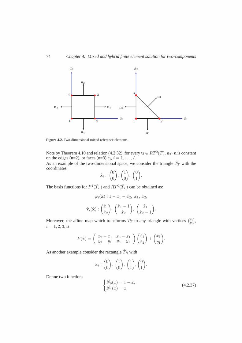
74 Chapter 4. Mixed and hybrid finite element solution for two-components
x1x1
x2x2
n1
n1 n2
n2
n3
n3
n4
11 22
334
Figure 4.2.Two-dimensional mixed reference elements.
Note by Theorem 4.10 and relation (4.2.32), for everyu ∈ RT 0(T ), nT ·u is constanton the edges (n=2), or faces (n=3)ei, i = 1, . . . , I.As an example of the two-dimensional space, we consider the triangleTT with thecoordinates
xi :
(0
0
),
(1
0
),
(0
1
).
The basis functions forP 1(TT ) andRT 0(TT ) can be obtained as:
ϕi(x) : 1 − x1 − x2, x1, x2,
vi(x) :
(x1
x2
),
(x1 − 1
x2
),
(x1
x2 − 1
).
Moreover, the affine map which transformsTT to any triangle with vertices(xi
yi
),
i = 1, 2, 3, is
F (x) =
(x2 − x1 x3 − x1
y2 − y1 y3 − y1
)(x1
x2
)+
(x1
y1
).
As another example consider the rectangleTR with
xi :
(0
0
),
(1
0
),
(1
1
),
(0
1
).
Define two functions N0(x) = 1 − x,
N1(x) = x.(4.2.37)
4.2. A mixed variational formulation for the two-component model 75
Therefore, the basis function forP 1(T ) associated with the nodexi is
ϕi(x) = Nxi(1)(x1)Nxi(2)(x2).
The basis functions forRT 0(TR) associated withni, i = 1, 2, 3, 4, are
vi(x) :
(x1
0
),
(0
x2
),
(x− 1
0
),
(0
x2 − 1
),
respectively. Any parallelogramT with vertices(xi
yi
), i = 1, 2, 3, 4, can be defined
with the transformation
F (x) =
(x2 − x1 x4 − x1
y2 − y1 y4 − y1
)(x1
x2
)+
(x1
y1
).
In three-dimensional space, we consider two reference elements. Given a cube withthe coordinates
xi :
(000
),
(100
),
(110
),
(010
),
(001
),
(101
),
(111
),
(011
),
then the basis function associated with the nodexi is taken as
ϕi(x) = Nxi(1)(x1)Nxi(2)(x2)Nxi(3)(x3).
The Raviart-Thomas basis function associated with the normal vectorni, i = 1, . . . , 6,is
vi :
(x1
00
),
(0x2
0
),
(00x3
),
(x1 − 1
00
),
(0
x2 − 10
),
(00
x3 − 1
).
The second example will be a tetrahedronTT with the coordinates
xi :
(000
),
(100
),
(010
),
(001
),
The basis functions forP 1(TT ) andRT 0(TT ) can be obtained as:
ϕi(x) : 1 − x1 − x2 − x3, x1, x2, x3.
and
vi : 2
(x1
x2
x3
), 2
(x1 − 1x2
x3
), 2
(x1
x2 − 1x3
), 2
(x1
x2
x3 − 1
).
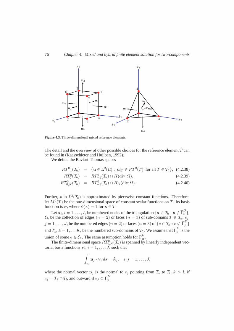
76 Chapter 4. Mixed and hybrid finite element solution for two-components
x1
x1x2
x2
x3x3
n1
n1 n2n2 n3
n3
n4
n4n5
n6
11
22 3
3
4
4
56
7
8
Figure 4.3.Three-dimensional mixed reference elements.
The detail and the overview of other possible choices for the referenceelementT canbe found in (Kaasschieter and Huijben, 1992).
We define the Raviart-Thomas spaces
RT 0−1(Th) = u ∈ L2(Ω) : u|T ∈ RT 0(T ) for all T ∈ Th, (4.2.38)
RT 00 (Th) = RT 0
−1(Th) ∩H(div; Ω), (4.2.39)
RT 00,N (Th) = RT 0
−1(Th) ∩HN (div; Ω). (4.2.40)
Further,p in L2(Th) is approximated by piecewise constant functions. Therefore,letM0(T ) be the one-dimensional space of constant scalar functions onT . Its basisfunction isψ, whereψ(x) = 1 for x ∈ T .
Letxi, i = 1, . . . , I, be numbered nodes of the triangulationx ∈ Th : x /∈ ΓDu ;
Eh be the collection of edges(n = 2) or faces(n = 3) of sub-domainsT ∈ Th; ej ,
j = 1, . . . , J , be the numbered edges(n = 2) or faces(n = 3) of e ∈ Th : e 6⊂ ΓDp
andTk, k = 1, . . .K, be the numbered sub-domains ofTh. We assume thatΓDp is the
union of somee ∈ Eh. The same assumption holds forΓDu .
The finite-dimensional spaceRT 00,N (Th) is spanned by linearly independent vec-
torial basis functionsvi, i = 1, . . . , J , such that∫
ej
nj · vi ds = δij , i, j = 1, . . . , J,
where the normal vectornj is the normal toej pointing fromTk to Tl, k > l, if
ej = Tk ∩ Tl, and outward ifej ⊂ ΓDp .
4.2. A mixed variational formulation for the two-component model 77
The multiplier spaceM0−1(Th) is defined as
M0−1(Th) = λ ∈ L2(Ω) : λ|T ∈M0(T ) for all T ∈ Th. (4.2.41)
Its basis functions areψk, k = 1, . . . ,K, such that
ψk(x) = δkl, x ∈ Tl, k, l = 1, . . . ,K. (4.2.42)
4.2.6 The resulting saddle point problem
The variational problem (4.2.2) is approximated by
(uh,qh, ph) ∈ (P 1D(Th))n ×RT 0
0,N (Th) ×M0−1(Th).
The functionsuh, qh andph are expressed as
uh(x, t) =I∑
i=1
ui(t)wi(x),
qh(x, t) =J∑
j=1
qj(t)vj(x)
ph(x, t) =K∑
k=1
pk(t)ψk(x).
Substitution in the discrete variational formulation, gives
Ady
dt+ By = F, (4.2.43)
where
A =
(0 0 00 0 0
BT 0 0
), B =
A 0 B0 C D
0 DT 0
and
y = [u, q, p]T ,
F = [F,0,0]T .
78 Chapter 4. Mixed and hybrid finite element solution for two-components
In the above formulation,
u = [u1 · · · , uI ]T ,
q = [q1, · · · , qJ ]T ,
p = [p1, · · · , pK ]T ,
Aij =
∫
Ω(2µsE(wi) : E(wj) + λs∇ · wi∇ · wj) dx,
Bij = −
∫
Ω∇ · wiψj dx,
Cij =1
K
∫
Ωvi · vj dx,
Dij = −
∫
Ω∇ · vjψi dx,
Fi =
∫
ΓNu
gNu · wi ds.
We shall use the implicit Euler scheme for time discretisation. Let∆t be the timestep and(uh,n,qh,n, ph,n) the approximation of the solution vector(uh,qh, ph) att = tn = n∆t. Then the system of equations resulting from backward Euler is
A 0 B0 ∆tC ∆tD
BT ∆tDT 0
(
un
qn
pn
)=
(F0
Bun−1
). (4.2.44)
Also it can be rewritten as(A B
BT 0
)((un, qn)T
pn
)=
((F,0)T
Bun−1
), (4.2.45)
where
A =
(A 00 ∆tC
), B =
(B
∆tD
). (4.2.46)
In (4.2.45), obviouslyA is symmetric positive definite because of he ellipticity ofbilinear formA. On the other hand, from the LBB condition it follows that the blockB has full rank. Indeed, ifp ∈ R
K such thatBp = 0, from LBB condition it followsthatB(wi,vj ; ph) = 0. Therefore
B(uh,qh; ph) = 0 for all (uh,qh) ∈ Vh × Wh,
and the LBB condition impliesph = 0, i.e., p = 0.From above we can see that the block matrix in (4.2.45) is symmetric and non-
singular. However, this matrix is not positive definite. Indeed, takep ∈ RK and set
w = ǫBp ∈ RI+J . Then we have
(w,p)
(A B
BT 0
)(wp
)= wT
Aw + 2wTBp = ǫpT
(ǫBT
AB + 2BTB)p.
(4.2.47)
4.3. Hybridization of the mixed method 79
The matrixBTB is symmetric positive definite andǫBT
AB is positive definite ifǫ > 0. If we chooseǫ < 0 with |ǫ| sufficiently small, the right-hand side of (4.2.47)becomes negative. This shows that the system is an indefinite system. More preciselywe have the following theorem.
Definition 4.11. LetA be a linear transformation onRn represented by a matrixA.If there is a vector0 6= x ∈ R
n such that
Ax = λx,
for some scalarλ, thenλ is called the eigenvalue ofA with corresponding (right)eigenvectorx. The eigenvalues of a matrixA are called its spectrum, and is denotedby spec(A).For a square matrixA, the square roots of the eigenvalues ofATA are called singu-lar values ofA.
Theorem 4.12. Let 0 < λmin ≤ λmax be the minimum and maximum eigenvaluesof A and let0 ≤ σmin ≤ σmax be the minimum and maximum singular values ofB.then we have
spec(
(A B
BT 0
)) ⊂ [µ−min, µ
−max] ∪ [µ+
min, µ+max], (4.2.48)
where
µ−min = 1/2(λmin −
√λ2
min + 4σ2max
)< 0
µ−max = 1/2(λmax −
√λ2
max + 4σ2min
)< 0
µ+min = λmin,
µ+max = 1/2
(λmax −
√λ2
max + 4σ2max
)> 0.
Proof. See (Rusten and Winther, 1992, Lemma 2.1).
4.3 Hybridization of the mixed method
Fraeijs de Veubeke (Fraeijs de Veubeke, 1965) and (Fraeijs de Veubeke, 1977) intro-duced a hybrid method for the mixed formulation in order to simplify the solution ofthe algebraic system that must be solved in the procedure. In Kaasschieter and Hui-jben (1992) a mixed-hybrid finite element discretisation is used to solve an importantclass of problems in mathematical physics that involves equations of the form
q = −A∇µ,
∇ · q = f,
whereA is a symmetric and uniformly positive definite second order tensor. It canbe seen that the mixed formulation of the above system leads to a saddle point prob-lem. Using the hybridization technique, the mixed finite element method results in a

80 Chapter 4. Mixed and hybrid finite element solution for two-components
system of linear equations with a sparse and symmetric positive definite coefficientsmatrix.
Despite to this fact, the hybridization method reduces the number of degrees offreedom. Furthermore, in the computations we only have to compute inverses ofelement-wise block diagonal matrices.
In this section the hybridization technique is used for two-component model.First we introduce a hybridization procedure for the mixed formulation. Thiswillsimplify the solution of the algebraic system that must be solved in the procedure.The idea behind hybridization is to relax the continuity requirement for the variablesq. This will require to enlarge the Raviart-Thomas space in whichq is sought and tointroduce Lagrange multipliers to enforce the continuity of the normal component ofq across the inter-element boundaries.
Define
E∂h = e ∈ Eh : e ⊂ Γ. (4.3.1)
We assume thatΓDp is the union of somee ∈ E∂
h .The hybrid formulation will make use of Lagrangian multipliers belonging to the
spaceL2(Eh) that is defined to be the product space
L2(Eh) =∏
T∈Th
L2(∂T ). (4.3.2)
Recall thatM0(e), e ∈ Eh, is the space of constant functions one. Define themultiplier spaces
M0−1(Eh) = λ = (λe)e∈Eh
∈ H1/2(⋃
e∈Eh
e) : λe ∈M0(e) for all e ∈ Eh,
(4.3.3)
M0−1,D(Eh) = λ ∈M0
−1(Eh) : λ = 0 on ΓDp . (4.3.4)
The following lemma is an immediate consequence of the above definitions.
Lemma 4.13. Supposeq ∈ RT 0−1(Th), thenq ∈ RT 0
0,N (Th) if, and only if,
∑
T∈Th
∫
∂TλnT · q ds = 0 for all λ ∈M0
−1,D(Eh).
A spatial semi-discrete approximation by considering the hybridization techniqueis:
Find (uh,qh, ph, λh) (·, t) ∈ (P 1D(Th))n ×RT 0
−1(Th)×M0−1(Th)×M0
−1,D(Eh)
4.3. Hybridization of the mixed method 81
such that:
∫
Ω(2µsE(uh) : E(uh) + λs∇ · uh∇ · uh) dx −
∫
Ωph∇ · uh dx
=
∫
ΓNu
gNu · uh ds, (4.3.5a)
1
K
∫
Ωqh · qh dx −
∑
T∈Th
(∫
Tph∇ · qh dx −
∫
∂TλhnT · qh ds
)= 0,
(4.3.5b)
−∑
T∈Th
∫
T∇ · qhph dx −
∫
Ω
∂∇ · uh
∂tph dx = 0, (4.3.5c)
∑
T∈Th
∫
∂TnT · qhλh ds = 0, (4.3.5d)
for all test functions(uh, qh, ph, λh
)∈ (P 1
D(Th))n × RT 0−1(Th) × M0
−1(Th) ×M0
−1,D(Eh) andt > 0.
Letxi, i = 1, . . . , I, be numbered nodes of the triangulationx ∈ Th : x /∈ ΓDu ;
Tk, k = 1, . . . ,K, be numbered sub-domains ofTh ande(T )j , j = 1, . . . , J (T ), be the
edges(n = 2) or faces(n = 3) of T for eachT ∈ Th.Recall that the finite-dimensional spaceRT 0
−1(Th) is spanned by linearly inde-
pendent vectorial basis functionsv(T )j , j = 1, . . . , J (T ), T ∈ Th, such thatv(T )
j hasits support inT and
∫
e(T )
j′
nt · v(T )j ds = δjj′ , j, j′ = 1, . . . , J (T ).
Thus a functionq ∈ RT 0−1(Th) hasJ (T ) degrees of freedom per sub-domainT ∈ Th
and in totalJ =∑
T∈ThJ (T ) degrees of freedom inTh. The degrees of freedom of
q in the sub-domainT ∈ Th are equal to∫
e(T )j
nT · q ds, j = 1, . . . J (T ).
Recall that the finite-dimensional spaceM0−1(Th) is spanned by the linearly indepen-
dent scalar basis functionsψk, k = 1, . . . ,K, such that (4.2.42) holds.Let el, l = 1, . . . , L, be the numbered edges(n = 2) or faces(n = 3) of
e ∈ Eh : e 6⊂ ΓDp . The finite-dimensional spaceM0
−1,D(Eh) is spanned by thelinearly independent scalar basis functionsηl, l = 1, . . . , L, such that
ηl(x) = δll′ , x ∈ el′ , l, l′ = 1, . . . , L.
82 Chapter 4. Mixed and hybrid finite element solution for two-components
Therefore a functionλ ∈ M0−1,D(Eh) has one degree of freedom per edgeel, l =
1, . . . , L, which is equal to its constant value onek.Now by definition, functionsuh, qh, p andλh are expressed as
uh(x, t) =I∑
i=1
ui(t)wi(x),
qh(x, t) =J∑
j=1
qj(t)vj(x),
ph(x, t) =
K∑
k=1
pk(t)ψk(x),
λh(x, t) =L∑
ℓ=1
λℓ(t)ηl(x).
Substituting this in the mixed-hybrid variational formulation gives
Ady
dt+ By = F, (4.3.6)
whereA andB are
A =
0 0 0 00 0 0 0
BT 0 0 00 0 0 0
, B =
A 0 B 00 C DE0 DT 0 00 ET 0 0
and
F = [F,0,0,0]T ,
y =[u, q, µ, λ
]T.
In the above formulations,
u = [u1 · · · , unI ]T ,
q = [q1, · · · , qJ ]T ,
p = [p1, · · · , pK ]T ,
λ = [λ1, · · · , λL]T ,
Aij =
∫
Ω(2µsE(wi) : E(wj) + λs∇ · wi∇ · wj) dx,
Bij = −
∫
Tj
∇ · wi dx,
Cij =1
K
∫
Ωvi · vj dx,
Dij = −
∫
Tj
∇ · vi dx,
4.3. Hybridization of the mixed method 83
Eik =
∫
ek
ni · vi ds,
Fi =
∫
ΓNu
gNu · wi ds.
Theorem 4.14. (D|E)TC−1(D|E) is a symmetric positive definite matrix.
Proof. C is symmetric positive definite and(D|E)TC−1(D|E) is symmetric posi-tive semi-definite. To prove the positive-definiteness, we need to show that (D|E)has full rank. Suppose
(D|E)(p, λ
)T= 0 ⇒ Dp + Eλ = 0.
But
Dp + Eλ = 0 ⇔ vT (Dp + Eλ) = 0 for all v ∈ RJ
⇔∑
T∈Th
(∫
Tph∇ · vh dx −
∫
∂TλhnT · vh ds
)= 0 for all vh ∈ RT 0
−1(Th)
⇔∑
T∈Th
∫
∂T(ph − λh)nT · vh ds = 0 for all vh ∈ RT 0
−1(Th)
⇔ ph = λh on∂T for all T ∈ Th ⇔ ph = 0 in Ω, λh = 0 on⋃e
e∈Eh
⇔ p = 0, λ = 0,
Therefore we have(Dp + Eλ
)TC−1
(Dp + Eλ
)> 0 (4.3.7)
for all (p, λ) ∈ RK+L\0.
In the sequel the hybridization technique will be proceeded. Note that the system(4.3.6) can be considered as
Au + Bpl = F,
Cq + (D|E)
(p
λ
)= 0,
(BT
0
)d
dtu + (D|E)T q =
(0
0
) (4.3.8)
In the system (4.3.8)C is a symmetric positive definite matrix and can be inverted atthe finite element level. Therefore the second equation in (4.3.8) implies
q = −C−1(D|E)
(p
λ
). (4.3.9)
84 Chapter 4. Mixed and hybrid finite element solution for two-components
Using (4.3.9) and the third equation in (4.3.8) we get(
BT
0
)d
dtu − (D|E)TC−1(D|E)
(p
λ
)=
(00
). (4.3.10)
In the next step we solve the above equation forp. To do this, we need to state thefollowing lemma.
Lemma 4.15. DTC−1D is a symmetric positive definite matrix.
Proof. SinceC is a symmetric positive definite matrix,DTC−1D is symmetric pos-itive semi-definite. In order to prove that this matrix is positive definite, we need tofind the null space of it.Let Dp = 0, then
∑
T∈Th
∫
Tph∇ · vh dx = 0 for all vh ∈ RT 0
−1(Th).
vh is assumed to be continuous inside each elementT , therefore the above summa-tion will reduce to each elementT . With an appropriate choice ofvh, we can take∇ · vh to be equal to 1 inT , therefore we have
∫
Tph dx = 0 for all T ∈ Th.
Henceph|T = 0 for all T ∈ Th.
This results in the symmetric positive definiteness ofDTC−1D.
Now by applying the above lemma,p can be derived as
p = (DTC−1D)−1
(−DTC−1Eλ + BT d
dtu
). (4.3.11)
If we substitute (4.3.11) in system (4.3.10), then this system reduces to
(Au0
)+
(A1 A2
AT2 −A3
)(ddt u
λ
)=
(F0
), (4.3.12)
whereA1,A1 andA3 are
A1 = B(DTC−1D)−1BT , (4.3.13)
A2 = −B(DTC−1D)−1DTC−1E, (4.3.14)
A3 = −ETC−1D(DTC−1D)−1DTC−1E + ETC−1E.
(4.3.15)
4.4. Numerical Simulations 85
Remark 4.16. Note that in computation ofA1, A2 andA3, the inverse of the matrixDC−1D is needed.
Remark 4.17. From Theorem 4.14 it follows that
ηT A3η = (Dη1 + Eη2)T
C−1 (Dη1 + Eη2) > 0 for all η2 ∈ RK\0,
(4.3.16)where
η1 = −(DC−1D)−1DTC−1Eη2, η = (η1,η2).
ThereforeA3 is a symmetric positive definite matrix.
Remark 4.18. By using the above remark, we can take one more step to solve thesystem for
λ = A−13 AT
2 u, (4.3.17)
hence the system(4.3.12)is reduced to
(A1 + A2A
−13 AT
2
) ddt
u + Au = F. (4.3.18)
Letting∆t be the time step and(un, λn) the approximation of the solution vector(u, λ) at t = tn = n∆t. Then the nonlinear system of equations (4.3.12) resultingfrom backward Euler is:
(A + A1/∆t A2
AT2 −∆tA3
)(un+1
λn+1
)=
(F + A1un/∆t
AT2 un
). (4.3.19)
Remark 4.19. Frijns (Frijns, 2001, page 54) has shown that oscillations in the solu-tion of discretised system
(A1 + A2A
−13 AT
2 + ∆tA)un+1 = ∆tF +
(A1 + A2A
−13 AT
2
)un+1
can occur when matrixA1 +A2A−13 AT
2 +∆tA is not an M-matrix. This matrix willbe an M-matrix if
∆t > ∆tcrit =h2
6K(2µs + λs), (4.3.20)
whereh is the mesh size.
4.4 Numerical Simulations
In this section the element contributions to the matrices and right-hand sides in(4.3.12) are computed. Remember the given triangulationTh of Ω and the referenceelementT in (4.2.21).
86 Chapter 4. Mixed and hybrid finite element solution for two-components
The element contribution to the elasticity matrixA andB can be calculated ina standard way. To calculate the element contribution to the matricesC we need toconsider the following analysis. Considering (4.2.31) we have
(C
(T )
J(T )×J(T )
)
ij=
∫
Tv
(T )i · v
(T )j dx =
∫
TC(T )vi · vjd x, (4.4.1)
whereC(T )(x) = (detBn)−1BT
nBn
andvi(x) = (detBn)B−1
n v(T )i (x), x ∈ T.
Note that the local basis functionsvi, i = 1, ..., J (T ), only depend on the referenceelementT . If the notations
vi(x) = [vik(x)]k=1,...,n and C(T ) =[c(T )kl
]
k,l=1,...,n
are used, then ∫
TC(T )vi · vjdx =
n∑
k=1
n∑
l=1
c(T )kl (Akl)ij , (4.4.2)
where the matrices ((Akl)J(T )×J(T )
)ij
=
∫
Tvikvjl dx (4.4.3)
only depend on the reference elementT . Note thatc(T )kl = c
(T )lk andAkl = Alk, thus
(C
(T )
J(T )×J(T )
)
ij=
n∑
k=1
c(T )kk (Akk)ij +
n∑
k=1
n−1∑
l=1
c(T )kl (Akl + Alk)ij , (4.4.4)
where all matrices in the summations are symmetric. In (Kaasschieter and Huijben,1992) an overview of the matricesAkk andAkl + Alk, k 6= l, corresponding tovarious choice of the reference elementT is given.
Using Green’s formula, (4.2.30) and (4.2.35), simple formulas can be derived forthe element contributions of the remaining matrices and right-hand sides in (4.3.12),namely
(D
(T )
J(T )×1
)
i= −
∫
T∇ · v
(T )i dx = −1,
(E
(T )
J(T )×J(T )
)
ik=
∫
e(T )k
nT · v(T )i ds = δik,
(4.4.5)
The computation of(DTC−1D)−1 is essential when determining the matricesAi,(i = 1, 2, 3) in (4.3.13)-(4.3.15). This matrix is a diagonal matrix and it can thus becomputed at the finite element level. The matricesAi are obtained by assemblingtheir element contributions.
4.4. Numerical Simulations 87
4.4.1 Example 1: One-dimensional confined compression problem
In this section the numerical solutions are calculated for given examples. Toverifythe method, solutions are compared with the analytical solutions from chapter 3.
A one-dimensional confined compression experiment is considered. Thehomo-geneous sample with the diameter of 4 mm and the height of approximatelyL = 1mm is put in an insulating conforming ring. A piston on the top of the sample isloaded mechanically. Figure 4.4 illustrate the experimental setup. In this experiment,we apply load on the piston to be equal tof(t) = −f0H(t− t0), with H(t− t0) theHeaviside function andf0 > 0. The following parameters are taken:
Parameter Unit Value2µs + λs MPa 4 × 10³
K m4 N−1 s−1 1.0 × 10⁻¹⁸
ϕ 0.7f0 MPa 5
Table 4.1.Material parameters
We use a rectangle in which only vertical displacement (direction of force)is allowedwith 40 vertical elements and one horizontal element. The variation of water pres-sure, displacement along they axis and the fluid flow are shown in Figure 4.4. Fort → t+o , the pressure shows a large gradients. This is due to the fact that the Dirich-let boundary conditionp = 0 at y = L contradicts with the asymptotic behaviourp → f0 ast → t+0 . Frijns (Frijns, 2001, page 54) has shown that the time step in-fluences the choice of an initial grid. In fact, the time step should be larger than thecritical time step using above material parameters
∆t ≥ ∆critt =h2
y
6K(2µs + λs).
This shows that to have a smaller time step we do need to refine our mesh. TheL2-norm for the global error in the displacement solution at the final time are alsocalculated and it appears that the error isO(∆t) andO(h2) (Frijns, 2001).
4.4.2 Example 2: Two-dimensional footing problem
The second example is a two-dimensional footing problem as given in (Murad andLoula, 1994). The simulation domain is a8 × 5 mm block of porous medium. Atthe basis of this domain the medium is assumed to be fixed and impervious, whileat the upper left part of the domain (fourth of the total length) we apply loadon thef(t) = −f0H(t− t0), with H(t− t0) the Heaviside function andf0 = 5 MPa.
The material parameters are taken like the consolidation problem from table 4.1.The mixed hybrid finite element uses the non-uniform grid which is more refined near
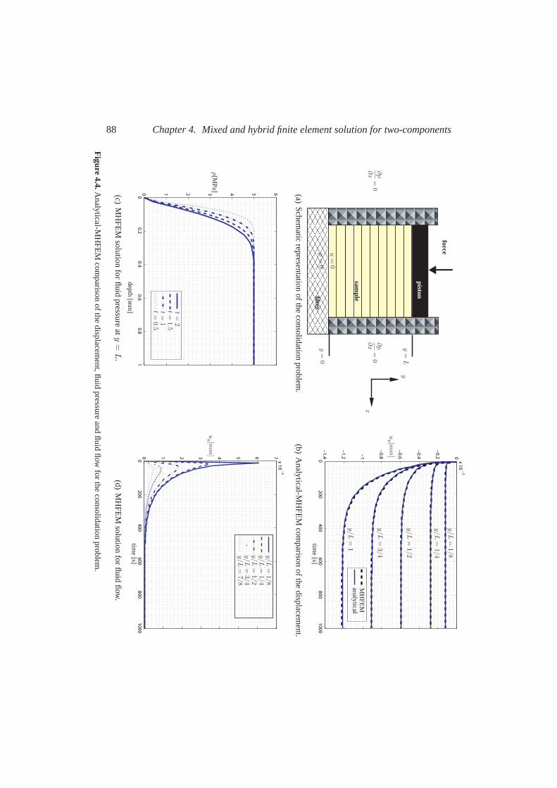
88 Chapter 4. Mixed and hybrid finite element solution for two-components
force
piston
samplefilter
x
y
u=
0
p=
0y
=0
y=
L
∂p
∂x
=0
∂p
∂x
=0
(a)S
chematic
representationofthe
consolidationproblem
.
02
00
40
06
00
80
01
00
0−
1.4
−1
.2
−1
−0
.8
−0
.6
−0
.4
−0
.2 0x 1
0−
3
y/L
=1/8
y/L
=1/4
y/L
=1/2
y/L
=3/4
y/L
=1
time
[s]
uy [m
m]
MH
FE
Manalytical
(b)A
nalytical-MH
FE
Mcom
parisonofthe
displacement.
00
.20
.40
.60
.81
0 1 2 3 4 5 6
depth[m
m]
p[MP
a]
t=
2t=
1.5t=
1t=
0.5
(c)M
HF
EM
solutionfor
fluidpressure
aty=L
.
02
00
40
06
00
80
01
00
00 1 2 3 4 5 6 7
x 10
−5
y/L
=1/8
y/L
=1/4
y/L
=1/2
y/L
=3/4
y/L
=7/8
time
[s]
uy [m
m]
(d)M
HF
EM
solutionfor
fluidflow
.
Figure
4.4.Analytical-M
HF
EM
comparison
ofthedisplacem
ent,fluidpressure
andflu
idflow
forthe
consolidationproblem
.
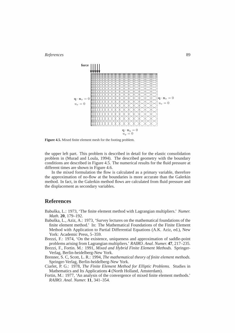
References 89
q · nx = 0q · nx = 0
q · ny = 0
ux = 0ux = 0
uy = 0
force
Figure 4.5.Mixed finite element mesh for the footing problem.
the upper left part. This problem is described in detail for the elastic consolidationproblem in (Murad and Loula, 1994). The described geometry with the boundaryconditions are described in Figure 4.5. The numerical results for the fluid pressure atdifferent times are shown in Figure 4.6.
In the mixed formulation the flow is calculated as a primary variable, thereforethe approximation of no-flow at the boundaries is more accurate than the Galerkinmethod. In fact, in the Galerkin method flows are calculated from fluid pressure andthe displacement as secondary variables.
References
Babuska, L.: 1973, ‘The finite element method with Lagrangian multipliers.’Numer.Math.20, 179–192.
Babuska, L., Aziz, A.: 1973, ‘Survey lectures on the mathematical foundations of thefinite element method.’ In: The Mathematical Foundations of the Finite ElementMethod with Application to Partial Differential Equations (A.K. Aziz, ed.), NewYork: Academic Press, 5–359.
Brezzi, F.: 1974, ‘On the existence, uniqueness and approximation of saddle-pointproblems arising from Lagrangian multipliers.’RAIRO. Anal. Numer.47, 217–235.
Brezzi, F., Fortin. M.: 1991,Mixed and Hybrid Finite Element Methods.Springer-Verlag, Berlin-heidelberg-New York.
Brenner, S. C, Scott, L. R.: 1994,The mathematical theory of finite element methods.Springer-Verlag, Berlin-heidelberg-New York.
Ciarlet, P. G.: 1978,The Finite Element Method for Elliptic Problems.Studies inMathematics and Its Applications4 (North Holland, Amsterdam).
Fortin, M.: 1977, ‘An analysis of the convergence of mixed finite element methods.’RAIRO. Anal. Numer.11, 341–354.
90 Chapter 4. Mixed and hybrid finite element solution for two-components
Fraeijs de Veubeke, B. X.: 1965, ‘Displacement and equilibrium models in thefiniteelement method.’In “Stress Analysis”, O. C. Zienkiewicz and G. Holister (eds.),John Wiley, New York.
Fraeijs de Veubeke, B. X.: 1977, ‘An analysis of the convergence of mixed finiteelement methods.’RAIRO. Anal. Numer.11, 341–354.
Frijns, A. J. H., Huyghe, J. M., Janssen, J. D.: 1997, ‘A validation of thequadriphasicmixture theory for intervertebral disc tissue.’Int. J. Engineering Science.35, 1419–1429.
Frijns, A. J. H.: 2001,A four-component mixture theory applied to cartilaginoustissues.PhD-thesis, Eindhoven University of Technology.
Kaasschieter, E. F., Huijben, A. J. M.: 1992, ‘Mixed-hybrid finite elementsandstreamline computation for the potential flow problem.’Numer. Methods PartialDiffer. Equat.8, 221–266.
Kaasschieter, E. F., Frijns, A. J. H., Huyghe, J. M.: 2003 ‘Mixed finite elementmodelling of cartilaginous tissues.’Mathematics and Computers in Simulation.61, 549–560.
Lewis, R. W., Schrefler, B. A.: 1998,The finite element method in the static anddynamic deformation and consolidation of porous media.Wiley.
van Loon, R., Huyghe, J. M., Wijlaars, M. W., Baaijens, F. P. T.: 2003, ‘3D FEimplementation of an incompressible quadriphasic mixture model.’InternationalJournal for Numerical Methods in Engineering57, 1243–1258.
Murad, M., Loula, A.: 1992, ‘Improved accuracy in finite element analysisof Biot’sconsolidation problem.’Comput. Methods. Appl. Mech. Engrg.95, 359–382.
Murad, M., Loula, A.: 1994, ‘On stability and convergence of finite elementap-proximations of Biot’s consolidation problem.’Intern. J. Numer. Meth. Engrg.37,645–667.
Murad, M., Thomee, V. ,Loula, A.: 1996, ‘Asymptotic behavior of semidiscretefinite-element approximations of Biot’s consolidation problem.’SIAM. J. Numer.Anal.33, 1065–1083.
Nedelec, J. C.: 1980, ‘Mixed finite elements inR3.’ Numer. Math.35, 315–341Nedelec, J. C.: 1986, ‘A new familiy of mixed finite elements inR
3.’ Numer. Math.50,57–81
Raviart, P. A., Thomas, J. M.: 1977 ‘A mixed finite element method for 2nd-orderelliptic problems.’Mathematical Aspects of Finite Element Methods, Lecture Notein Mathematics, I. Galligani and E. Magenes, Eds., Springer, BerlinVol 606, 292–315.
Roberts, J. E., Thomas, J. M.: 1991, ‘Mixed and hybrid finite element methods.’Handbook of Numerical Analysis, Volume II: Finite Element Methods,P.G. Ciarletand J.L. Lions, Eds., North Holland, Amsterdam, 523–639.
Rusten, T., Winther, R.: 1992, ‘A Preconditioned Iterative Method for SaddlepointProblems.’SIAM. J. Mat. Anal. Appl.13No 3, 887–904.
Thomas, J. M.: 1977,Sur l’analyse numerique des methods d’elements finis hybridset mixtes.Ph.D. thesis, University Pierre et Marie Curie, Paris.
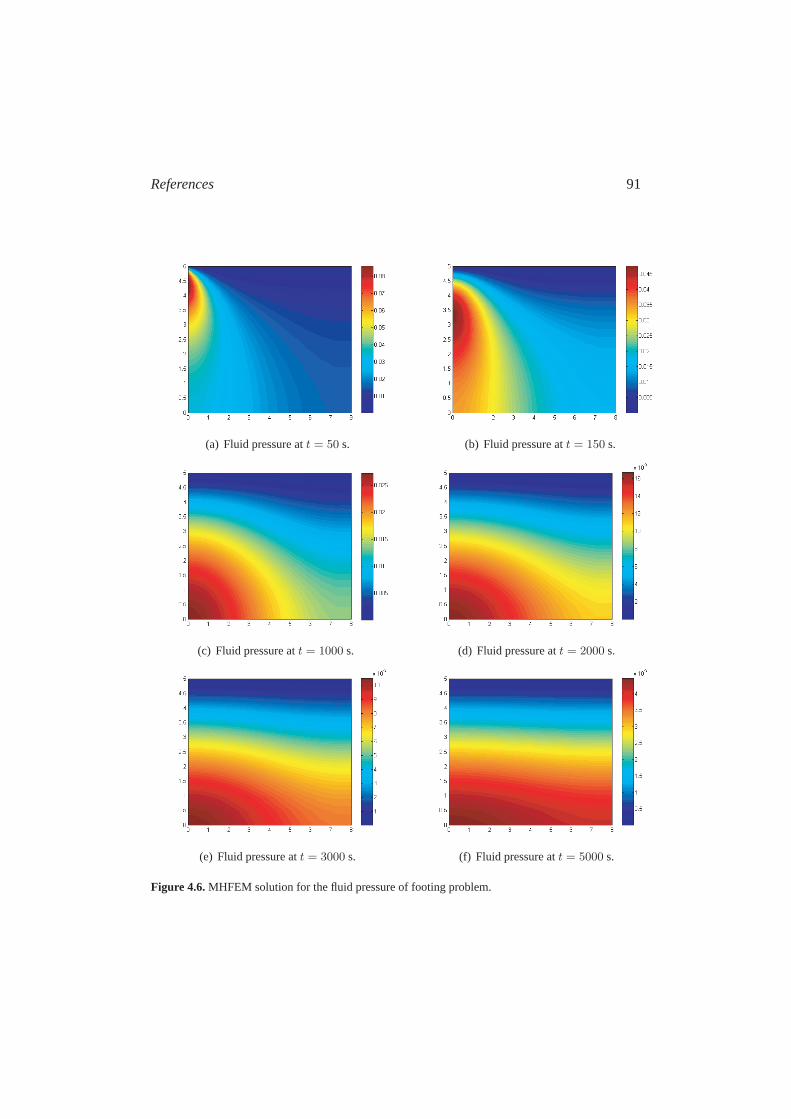
References 91
(a) Fluid pressure att = 50 s. (b) Fluid pressure att = 150 s.
(c) Fluid pressure att = 1000 s. (d) Fluid pressure att = 2000 s.
(e) Fluid pressure att = 3000 s. (f) Fluid pressure att = 5000 s.
Figure 4.6.MHFEM solution for the fluid pressure of footing problem.


Chapter 5
Mixed and hybrid finite element solution forfour-component
⋆
I n the previous section we gave a detailed overview on the mixed formulation forthetwo-component model. The solid-fluid interactions cannot describe the osmotic
effects, which have a major influence on the behaviour of tissues. Therefore theobjective of this chapter is to study the mixed variational formulation to derive asetof solutions for four-component model given in chapter 2.
Like the two-component model, also here it is desirable to obtain approximationsof the fluid flow and ions flow that fulfil the conservation equations.
In finite element simulation (van Loon et al., 2003), (Ehlers et al., 2005a), (Ehlerset al., 2005b) and (Ehlers et al., 2006) these quantities are computed by differentiationof the electro-chemical potential solutions. This approach may lead to violationofthe mass conservation principle.
The mixed finite element method provides an attractive framework for this typeof problems by simultaneously approximating flows and electro-chemical potentials.Flows computed by mixed finite elements automatically satisfy the “divergence free”property, both locally and globally, and the corresponding normal flux field is guar-anteed to be continuous across inter-element boundaries. The mixed finite elementmethod has been extensively used for the solution of parabolic equations arising indifferent application fields. The mixed finite element method was proposed for two-dimensional problems by (Raviart and Thomas, 1977), (Thomas, 1977) and (Robertsand Thomas, 1991), and by Nedelec for three-dimensional problems (Nedelec, 1980)and (Nedelec, 1986). In this article the mixed finite element variational formulationis derived for the set of coupled equations in general dimensions. Only the lowest-order mixed method will be considered, first, because higher order-methods resultin some conceptual complications and, second, because the lowest-ordermethod iscomparatively easy and straightforward to use for practical problems.
In steady-state flow problems, i.e., elliptic equations, the system derived frommixed formulation becomes indefinite. A common solution method discussed in the
⋆ Parts of this chapter will be appeared in ESAIM: Mathematical Modelling andNumerical Analysis(Malakpoor et al., 2006b)
93
94 Chapter 5. Mixed and hybrid finite element solution for four-component
previous chapter is the so-called mixed-hybrid finite element (MHFEM) technique.Through the definition of an extra variable representing the pressure atelement edges,MHFEM gives rise to a symmetric positive definite matrix with good conditioningproperties. Using the MHFEM technique for our model, we still have an indefinitesystem but the advantage is that the number of degrees of freedom will bereduced.In fact, for a three-dimensional problem this number will be reduced from15 to 6degrees of freedom. Note that in our case the equations are time dependent and non-linear, therefore a choice for time integration and a nonlinear solver is needed. We usesome techniques to tackle this problem. In chapter 3 analytical solutions are givenfor linearised problem. Finally the results are validated for confined consolidationand free swelling experiments using the analytical solution.
5.1 The coupled mixed formulation
Remember that,
1. In four-component mixture theory a deformable and charged porousmediumis saturated with a fluid with dissolved cations and anions.
2. The solid skeleton and fluid are assume to be intrinsically incompressible.
3. We assume that no chemical reactions exist between phases and no sources orsinks exist.
4. We neglect the inertia effects and body forces.
5. The materials are assumed to be isothermal.
6. The mixture is assumed to be saturated, i.e., (2.2.1) holds.
7. It is assumed that the solid matrix is entirely elastic and initially isotropic.
8. We assume infinitesimal deformation for the solid phase.
Let Ω be an open domain inRn, n = 1, 2, 3. DefineΩT = Ω × (0, T ] for T > 0,and consider the setsΓD
u andΓNu (and similarlyΓD
p andΓNp ) to be two disjoint open
subsets of the total boundaryΓ = ∂Ω, such thatΓDα ∩ΓN
α = ∅ andΓDα ∪ ΓN
α = Γ forα = u andp. We assume measΓD
α > 0 for α = u, p.Remember the definitions of the spacesHD
1 (Ω), V andHN (div; Ω) in section4.1:
V =u ∈ (H1(Ω))n : u = 0 onΓD
u
H1D(Ω) =
ϕ ∈ H1(Ω) : ϕ = 0 onΓD
p
,
HN (div; Ω) =q ∈ H(div; Ω) : n · q = 0 onΓN
p
,
H−1/2N (Γ) =
µ ∈ H−1/2(Γ) : µ = 0 onΓN
p
.
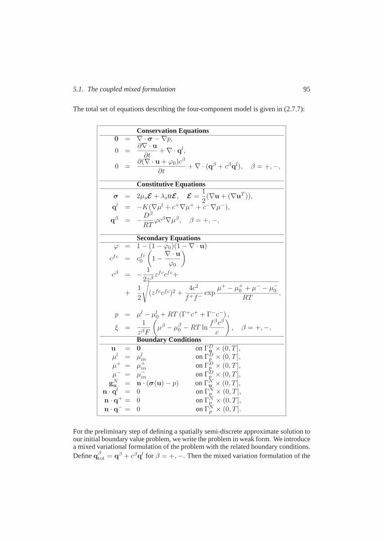
5.1. The coupled mixed formulation 95
The total set of equations describing the four-component model is givenin (2.7.7):
Conservation Equations0 = ∇ · σ −∇p,
0 =∂∇ · u
∂t+ ∇ · ql,
0 =∂(∇ · u + ϕ0)c
β
∂t+ ∇ · (qβ + cβql), β = +,−,
Constitutive Equations
σ = 2µsE + λstrE , E =1
2(∇u + (∇uT )),
ql = −K(∇µl + c+∇µ+ + c−∇µ−),
qβ = −Dβ
RTϕcβ∇µβ , β = +,−,
Secondary Equationsϕ = 1 − (1 − ϕ0)(1 −∇ · u)
cfc = cfc0
(1 −
∇ · u
ϕ0
)
cβ = −1
2zβzfccfc+
+1
2
√
(zfccfc)2 +4c2
f+f−exp
µ+ − µ+0 + µ− − µ−0RT
,
p = µl − µl0 +RT (Γ+c+ + Γ−c−) ,
ξ =1
zβF
(µβ − µβ
0 −RT lnfβcβ
c
), β = +,−,
Boundary Conditionsu = 0 onΓD
u × (0, T ],µl = µl
in onΓDp × (0, T ],
µ+ = µ+in onΓD
p × (0, T ],
µ− = µ−in onΓDp × (0, T ],
gNu = n · (σ(u) − p) onΓN
u × (0, T ],n · ql = 0 onΓN
p × (0, T ],
n · q+ = 0 onΓNp × (0, T ],
n · q− = 0 onΓNp × (0, T ].
For the preliminary step of defining a spatially semi-discrete approximate solutiontoour initial boundary value problem, we write the problem in weak form. We introducea mixed variational formulation of the problem with the related boundary conditions.Defineq
βtot = qβ + cβql for β = +,−. Then the mixed variation formulation of the
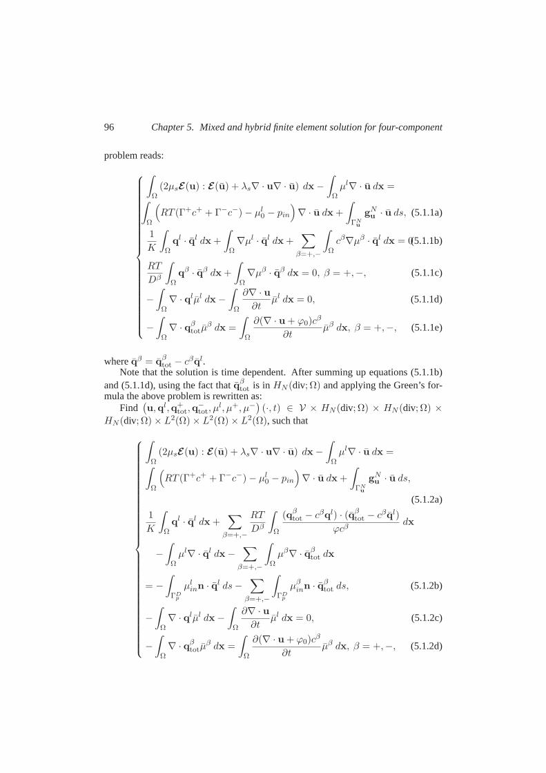
96 Chapter 5. Mixed and hybrid finite element solution for four-component
problem reads:
∫
Ω(2µsE(u) : E(u) + λs∇ · u∇ · u) dx −
∫
Ωµl∇ · u dx =
∫
Ω
(RT (Γ+c+ + Γ−c−) − µl
0 − pin
)∇ · u dx +
∫
ΓNu
gNu · u ds, (5.1.1a)
1
K
∫
Ωql · ql dx +
∫
Ω∇µl · ql dx +
∑
β=+,−
∫
Ωcβ∇µβ · ql dx = 0(5.1.1b)
RT
Dβ
∫
Ωqβ · qβ dx +
∫
Ω∇µβ · qβ dx = 0, β = +,−, (5.1.1c)
−
∫
Ω∇ · qlµl dx −
∫
Ω
∂∇ · u
∂tµl dx = 0, (5.1.1d)
−
∫
Ω∇ · qβ
totµβ dx =
∫
Ω
∂(∇ · u + ϕ0)cβ
∂tµβ dx, β = +,−, (5.1.1e)
whereqβ = qβtot − cβql.
Note that the solution is time dependent. After summing up equations (5.1.1b)and (5.1.1d), using the fact thatq
βtot is inHN (div; Ω) and applying the Green’s for-
mula the above problem is rewritten as:Find
(u,ql,q+
tot,q−tot, µ
l, µ+, µ−)(·, t) ∈ V × HN (div; Ω) × HN (div; Ω) ×
HN (div; Ω) × L2(Ω) × L2(Ω) × L2(Ω), such that
∫
Ω(2µsE(u) : E(u) + λs∇ · u∇ · u) dx −
∫
Ωµl∇ · u dx =
∫
Ω
(RT (Γ+c+ + Γ−c−) − µl
0 − pin
)∇ · u dx +
∫
ΓNu
gNu · u ds,
(5.1.2a)
1
K
∫
Ωql · ql dx +
∑
β=+,−
RT
Dβ
∫
Ω
(qβtot − cβql) · (qβ
tot − cβql)
ϕcβdx
−
∫
Ωµl∇ · ql dx −
∑
β=+,−
∫
Ωµβ∇ · qβ
tot dx
= −
∫
ΓDp
µlinn · ql ds−
∑
β=+,−
∫
ΓDp
µβinn · qβ
tot ds, (5.1.2b)
−
∫
Ω∇ · qlµl dx −
∫
Ω
∂∇ · u
∂tµl dx = 0, (5.1.2c)
−
∫
Ω∇ · qβ
totµβ dx =
∫
Ω
∂(∇ · u + ϕ0)cβ
∂tµβ dx, β = +,−, (5.1.2d)

5.1. The coupled mixed formulation 97
for all test functions(u, ql, q+
tot, q−tot, µ
l, µ+, µ−)∈ V×HN (div; Ω)×HN (div; Ω)×
HN (div; Ω) × L2(Ω) × L2(Ω) × L2(Ω) andt > 0. Note that the solution is timedependent.
Denote the triple(ql,q+tot,q
−tot) and(µl, µ+, µ−) by q andµ, respectively, and
define:
a(u, u) =
∫
Ω(2µsE(u) : E(u) + λs∇ · u∇ · u) dx,
b(u, µl) = −
∫
Ω∇ · uµl dx,
c(q, q) =1
K
∫
Ωql · ql dx +
∑
β=+,−
RT
Dβ
∫
Ω
(qβtot − cβql) · (qβ
tot − cβql)
ϕcβdx,
dl(ql, µl) = −
∫
Ω∇ · qlµl dx,
dβ(qβtot, µ
β) = −
∫
Ω∇ · qβ
totµβ dx, β = +,−,
F (u) =
∫
Ω
(RT (Γ+c+ + Γ−c−) − µl
0 − pin
)∇ · u dx +
∫
ΓNu
gNu · u ds,
F1(q) = −
∫
ΓDp
µlinn · ql −
∑
β=+,−
∫
ΓDp
µβinn · qβ
tot ds,
F β2 (µβ) =
∫
Ω(∇ · u + ϕ0)c
βµβ dx, β = +,−,
then the problem (5.1.2a) - (5.1.2d) can be rewritten as follows:
Findu,ql,q+
tot,q−
tot, µl, µ+, µ−
∈ V × HN (div; Ω) × HN (div; Ω)
×HN (div; Ω) × L2(Ω) × L2(Ω) × L2(Ω) such that
a(u, u) +b(u, µl) = F (u),
c(q, q) +dl(ql
, µl)+d
+(q+tot, µ
+)+d−(q−
tot, µ−)= F1(q),
d
dtb(u, µ
l) +dl(ql
, µl) = 0,
d+(q+
tot, µ+) =
d
dtF
+2 (µ+),
d−(q−
tot, µ−) =
d
dtF
−
2 (µ−),
(5.1.3)
for all test functions(u, ql, q+
tot, q−tot, µ
l, µ+, µ−)∈ V×HN (div; Ω)×HN (div; Ω)×
HN (div; Ω) × L2(Ω) × L2(Ω) × L2(Ω) andt > 0.We shall use the implicit Euler scheme for time discretisation. Let∆t be the time
step and(un,q
ln,q
+tot,n,q
−tot,n, µ
ln, µ
+n , µ
−n
)the approximation of the solution vector(
u,ql,q+tot,q
−tot, µ
l, µ+, µ−)
at t = tn = n∆t. Then the system of equation (5.1.3)resulting from backward Euler is:
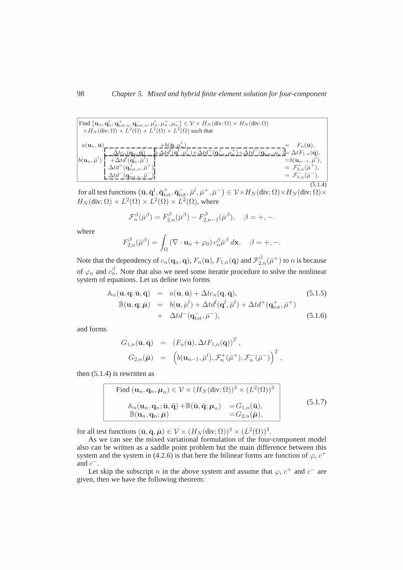
98 Chapter 5. Mixed and hybrid finite element solution for four-component
Findun,ql
n,q+tot,n,q−
tot,n, µln, µ+
n , µ−
n
∈ V × HN (div; Ω) × HN (div; Ω)
×HN (div; Ω) × L2(Ω) × L2(Ω) × L2(Ω) such that
a(un, u) +b(u, µln) = Fn(u),
∆tcn(qn, q) +∆tdl(ql
, µln)+∆td
+(q+tot, µ
+n )+∆td
−(q−
tot, µ−
n )= ∆tF1,n(q),b(un, µ
l) +∆tdl(ql
n, µl) =b(un−1, µ
l),∆td
+(q+tot,n, µ
+) = F+2,n(µ+),
∆td−(q−
tot,n, µ−) = F
−
2,n(µ−),
(5.1.4)for all test functions
(u, ql, q+
tot, q−tot, µ
l, µ+, µ−)∈ V×HN (div; Ω)×HN (div; Ω)×
HN (div; Ω) × L2(Ω) × L2(Ω) × L2(Ω), where
Fβn (µβ) = F β
2,n(µβ) − F β2,n−1(µ
β), β = +,−.
where
F β2,n(µβ) =
∫
Ω(∇ · un + ϕ0) c
βnµ
β dx, β = +,−.
Note that the dependency ofcn(qn, q), Fn(u), F1,n(q) andFβ2,n(µ+) ton is because
of ϕn andcβn. Note that also we need some iteratie procedure to solve the nonlinearsystem of equations. Let us define two forms
An(u,q; u, q) = a(u, u) + ∆tcn(q, q), (5.1.5)
B(u,q; µ) = b(u, µl) + ∆tdl(ql, µl) + ∆td+(q+tot, µ
+)
+ ∆td−(q−tot, µ
−), (5.1.6)
and forms
G1,n(u, q) = (Fn(u),∆tF1,n(q))T ,
G2,n(µ) =(b(un−1, µ
l),F+n (µ+),F−
n (µ−))T
,
then (5.1.4) is rewritten as
Find (un,qn,µn) ∈ V × (HN (div; Ω))3 × (L2(Ω))3
An(un,qn; u, q) +B(u, q; µn) =G1,n(u),B(un,qn; µ) =G2,n(µ),
(5.1.7)
for all test functions(u, q, µ) ∈ V × (HN (div; Ω))3 × (L2(Ω))3.As we can see the mixed variational formulation of the four-component model
also can be written as a saddle point problem but the main difference between thissystem and the system in (4.2.6) is that here the bilinear forms are function ofϕ, c+
andc−.Let skip the subscriptn in the above system and assume thatϕ, c+ andc− are
given, then we have the following theorem:
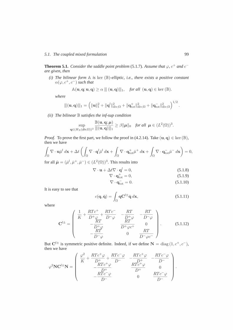
5.1. The coupled mixed formulation 99
Theorem 5.1. Consider the saddle point problem(5.1.7). Assume thatϕ, c+ andc−
are given, then
(i) The bilinear formA is ker (B)-elliptic, i.e., there exists a positive constantα(ϕ, c+, c−) such that
A(u,q;u,q) ≥ α 9 (u,q)91, for all (u,q) ∈ ker (B).
where
9(u,q)91 =(‖u‖2
1 + ‖ql‖2div;Ω + ‖q+
tot‖2div;Ω + ‖q−
tot‖2div;Ω
)1/2.
(ii) The bilinearB satisfies the inf-sup condition
supq∈(HN (div;Ω))3
B(u,q; µ)
9(u,q)91≥ β‖µ‖0 for all µ ∈ (L2(Ω))3.
Proof. To prove the first part, we follow the proof in (4.2.14). Take(u,q) ∈ ker (B),then we have∫
Ω∇ · uµl dx + ∆t
(∫
Ω∇ · qlµl dx +
∫
Ω∇ · q+
totµ+ dx +
∫
Ω∇ · q−
totµ− dx
)= 0,
for all µ = (µl, µ+, µ−) ∈ (L2(Ω))3. This results into
∇ · u + ∆t∇ · ql = 0, (5.1.8)∇ · q+
tot = 0, (5.1.9)
∇ · q−tot = 0. (5.1.10)
It is easy to see that
c(q, q) =
∫
ΩqCl±q dx, (5.1.11)
where
Cl± =
1
K+RTc+
D+ϕ+RTc−
D−ϕ−RT
D+ϕ−RT
D−ϕ
−RT
D+ϕ
RT
D+ϕc+0
−RT
D−ϕ0
RT
D−ϕc−
. (5.1.12)
But Cl± is symmetric positive definite. Indeed, if we defineN = diag (1, c+, c−),then we have
ϕ2NCl±N =
ϕ2
K+RTc+ϕ
D++RTc−ϕ
D−−RTc+ϕ
D+−RTc−ϕ
D−
−RTc+ϕ
D+
RTc+ϕ
D+0
−RTc−ϕ
D−0
RTc−ϕ
D−
.

100 Chapter 5. Mixed and hybrid finite element solution for four-component
In Lemma 3.2 we proved that this matrix is symmetric positive definite.Now let us continue the proof ofker (B)-ellipticity of the bilinear formA. Take
(u,q) ∈ ker (B), then by using Korn’s inequality (4.2.12) and equations (5.1.8) -(5.1.11) we have
A(u,q;u,q) = a(u,u) + ∆tc(q,q)
=
∫
Ω2µsE(u) : E(u) + λs(∇ · u)2 dx + ∆t
∫
Ω(ql,q+
tot,q−tot)C
l±
ql
q+tot
q−tot
≥ 2µsc‖u‖21 + λs‖∇ · u‖2
0 + C∆t(‖ql‖20 + ‖q+
tot‖20 + ‖q−
tot‖20)
≥ 2µsc‖u‖21 + λs(∆t)
2‖∇ · ql‖20 + C∆t(‖ql‖2
0 + ‖q+tot‖
2div;Ω + ‖q−
tot‖2div;Ω)
≥ α 9 (u,q)91, (5.1.13)
whereα = min (2µsc, λs(∆t)2, C) andC = C(ϕ, c+, c−).
To prove the second part (inf-sup condition), we restrict the supremumto a subset offunctions(0,q),
∆t supq∈(HN (div;Ω))3
dl(ql, µl) + d+(q+tot, µ
+) + d−(q−totµ
−)
‖q‖div;Ω≥ β‖µ‖0,
for all µ ∈ (L2(Ω))3. Easily it can be seen that the above supremum is greater orequal than
∆t supql∈HN (div;Ω)
dl(ql, µl)
‖ql‖div;Ω+ sup
q+tot∈HN (div;Ω)
d+(q+tot, µ
+)
‖q+tot‖div;Ω
+ supq−
tot∈HN (div;Ω)
d−(q−tot, µ
−)
‖q−tot‖div;Ω
.
In fact, we split the inf-sup condition to three inf-sup condition for each component,liquid, cation and anion. Following the proof for Theorem 4.4, we have a lower boundfor each of the above terms, therefore
∆t supq∈(HN (div;Ω))3
dl(ql, µl) + d+(q+tot, µ
+) + d−(q−tot, µ
−)
‖q‖div;Ω
≥ βl‖µl‖0 + β+‖µ+‖0 + β−‖µ−‖0
≥ β(‖µl‖2
0 + ‖µ+‖20 + ‖µ−‖2
0
)1/2
= β‖µ‖0. (5.1.14)
Therefore the inf-sup condition holds for allβ ≤ β. This proves the second part ofthe theorem.
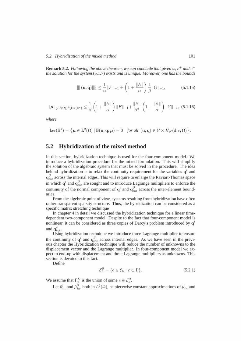
5.2. Hybridization of the mixed method 101
Remark 5.2. Following the above theorem, we can conclude that givenϕ, c+ andc−
the solution for the system(5.1.7)exists and is unique. Moreover, one has the bounds
9 (u,q)91 ≤1
α‖F‖−1 +
(1 +
‖A‖
α
)1
β‖G‖−1, (5.1.15)
‖µ‖(L2(Ω))3\ker(B∗) ≤1
β
(1 +
‖A‖
α
)‖F‖−1+
‖A‖
β2
(1 +
‖A‖
α
)‖G‖−1, (5.1.16)
where
ker(B∗) =µ ∈ L2(Ω) | B(u,q; µ) = 0 for all (u,q) ∈ V ×HN (div; Ω)
.
5.2 Hybridization of the mixed method
In this section, hybridization technique is used for the four-component model. Weintroduce a hybridization procedure for the mixed formulation. This will simplifythe solution of the algebraic system that must be solved in the procedure. The ideabehind hybridization is to relax the continuity requirement for the variablesql andq
βtot across the internal edges. This will require to enlarge the Raviart-Thomasspace
in whichql andqβtot are sought and to introduce Lagrange multipliers to enforce the
continuity of the normal component ofql andqβtot across the inter-element bound-
aries.From the algebraic point of view, systems resulting from hybridization haveoften
rather transparent sparsity structure. Thus, the hybridization can be considered as aspecific matrix stretching technique
In chapter 4 in detail we discussed the hybridization technique for a linear time-dependent two-component model. Despite to the fact that four-component model isnonlinear, it can be considered as three copies of Darcy’s problem introduced byql
andqβtot.
Using hybridization technique we introduce three Lagrange multiplier to ensurethe continuity ofql andq
βtot across internal edges. As we have seen in the previ-
ous chapter the Hybridization technique will reduce the number of unknowns to thedisplacement vector and the Lagrange multiplier. In four-component modelwe ex-pect to end-up with displacement and three Lagrange multipliers as unknowns. Thissection is devoted to this fact.
Define
E∂h = e ∈ Eh : e ⊂ Γ. (5.2.1)
We assume thatΓDp is the union of somee ∈ E∂
h .
Let µlin andµβ
in, both inL2(Ω), be piecewise constant approximations ofµlin and
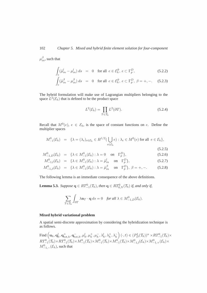
102 Chapter 5. Mixed and hybrid finite element solution for four-component
µβin, such that
∫
e(µl
in − µlin) ds = 0 for all e ∈ E∂
h , e ⊂ ΓDp , (5.2.2)
∫
e(µβ
in − µβin) ds = 0 for all e ∈ E∂
h , e ⊂ ΓDp , β = +,−. (5.2.3)
The hybrid formulation will make use of Lagrangian multipliers belonging to thespaceL2(Eh) that is defined to be the product space
L2(Eh) =∏
T∈Th
L2(∂T ). (5.2.4)
Recall thatM0(e), e ∈ Eh, is the space of constant functions one. Define themultiplier spaces
M0−1(Eh) = λ = (λe)e∈Eh
∈ H1/2(⋃
e∈Eh
e) : λe ∈M0(e) for all e ∈ Eh,
(5.2.5)
M0−1,D(Eh) = λ ∈M0
−1(Eh) : λ = 0 on ΓDp , (5.2.6)
M0−1,l(Eh) = λ ∈M0
−1(Eh) : λ = µlin on ΓD
p , (5.2.7)
M0−1,β(Eh) = λ ∈M0
−1(Eh) : λ = µβin on ΓD
p , β = +,−. (5.2.8)
The following lemma is an immediate consequence of the above definitions.
Lemma 5.3. Supposeq ∈ RT 0−1(Th), thenq ∈ RT 0
0,N (Th) if, and only if,
∑
T∈Th
∫
∂TλnT · q ds = 0 for all λ ∈M0
−1,D(Eh).
Mixed hybrid variational problem
A spatial semi-discrete approximation by considering the hybridization technique isas follows.
Find(uh,q
lh,q
+tot,h,q
−tot,h, µ
lh, µ
+h , µ
−h , λ
lh, λ
+h , λ
−h
)(·, t) ∈ (P 1
D(Th))n ×RT 0−1(Th)×
RT 0−1(Th)×RT 0
−1(Th)×M0−1(Th)×M0
−1(Th)×M0−1(Th)×M0
−1,l(Eh)×M0−1,+(Eh)×
M0−1,−(Eh), such that
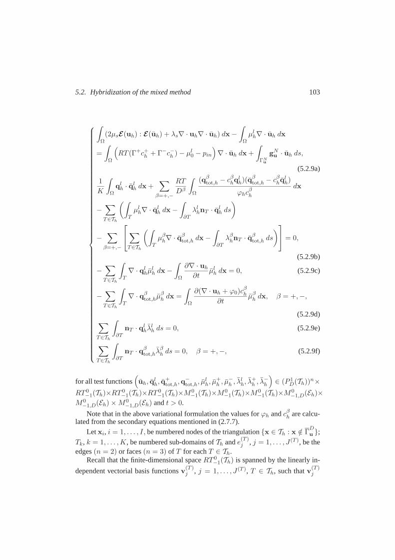
5.2. Hybridization of the mixed method 103
∫
Ω(2µsE(uh) : E(uh) + λs∇ · uh∇ · uh) dx −
∫
Ωµl
h∇ · uh dx
=
∫
Ω
(RT (Γ+c+h + Γ−c−h ) − µl
0 − pin
)∇ · uh dx +
∫
ΓNu
gNu · uh ds,
(5.2.9a)
1
K
∫
Ωql
h · qlh dx +
∑
β=+,−
RT
Dβ
∫
Ω
(qβtot,h − cβhq
lh)(qβ
tot,h − cβhqlh)
ϕhcβh
dx
−∑
T∈Th
(∫
Tµl
h∇ · qlh dx −
∫
∂Tλl
hnT · qlh ds
)
−∑
β=+,−
∑
T∈Th
(∫
Tµβ
h∇ · qβtot,h dx −
∫
∂Tλβ
hnT · qβtot,h ds
) = 0,
(5.2.9b)
−∑
T∈Th
∫
T∇ · ql
hµlh dx −
∫
Ω
∂∇ · uh
∂tµl
h dx = 0, (5.2.9c)
−∑
T∈Th
∫
T∇ · qβ
tot,hµβh dx =
∫
Ω
∂(∇ · uh + ϕ0)cβh
∂tµβ
h dx, β = +,−,
(5.2.9d)∑
T∈Th
∫
∂TnT · ql
hλlh ds = 0, (5.2.9e)
∑
T∈Th
∫
∂TnT · qβ
tot,hλβh ds = 0, β = +,−, (5.2.9f)
for all test functions(uh, q
lh, q
+tot,h,q
−tot,h, µ
lh, µ
+h , µ
−h , λ
lh, λ
+h , λ
−h
)∈ (P 1
D(Th))n×
RT 0−1(Th)×RT 0
−1(Th)×RT 0−1(Th)×M0
−1(Th)×M0−1(Th)×M0
−1(Th)×M0−1,D(Eh)×
M0−1,D(Eh) ×M0
−1,D(Eh) andt > 0.
Note that in the above variational formulation the values forϕh andcβh are calcu-lated from the secondary equations mentioned in (2.7.7).
Letxi, i = 1, . . . , I, be numbered nodes of the triangulationx ∈ Th : x /∈ ΓDu ;
Tk, k = 1, . . . ,K, be numbered sub-domains ofTh ande(T )j , j = 1, . . . , J (T ), be the
edges(n = 2) or faces(n = 3) of T for eachT ∈ Th.Recall that the finite-dimensional spaceRT 0
−1(Th) is spanned by the linearly in-
dependent vectorial basis functionsv(T )j , j = 1, . . . , J (T ), T ∈ Th, such thatv(T )
j
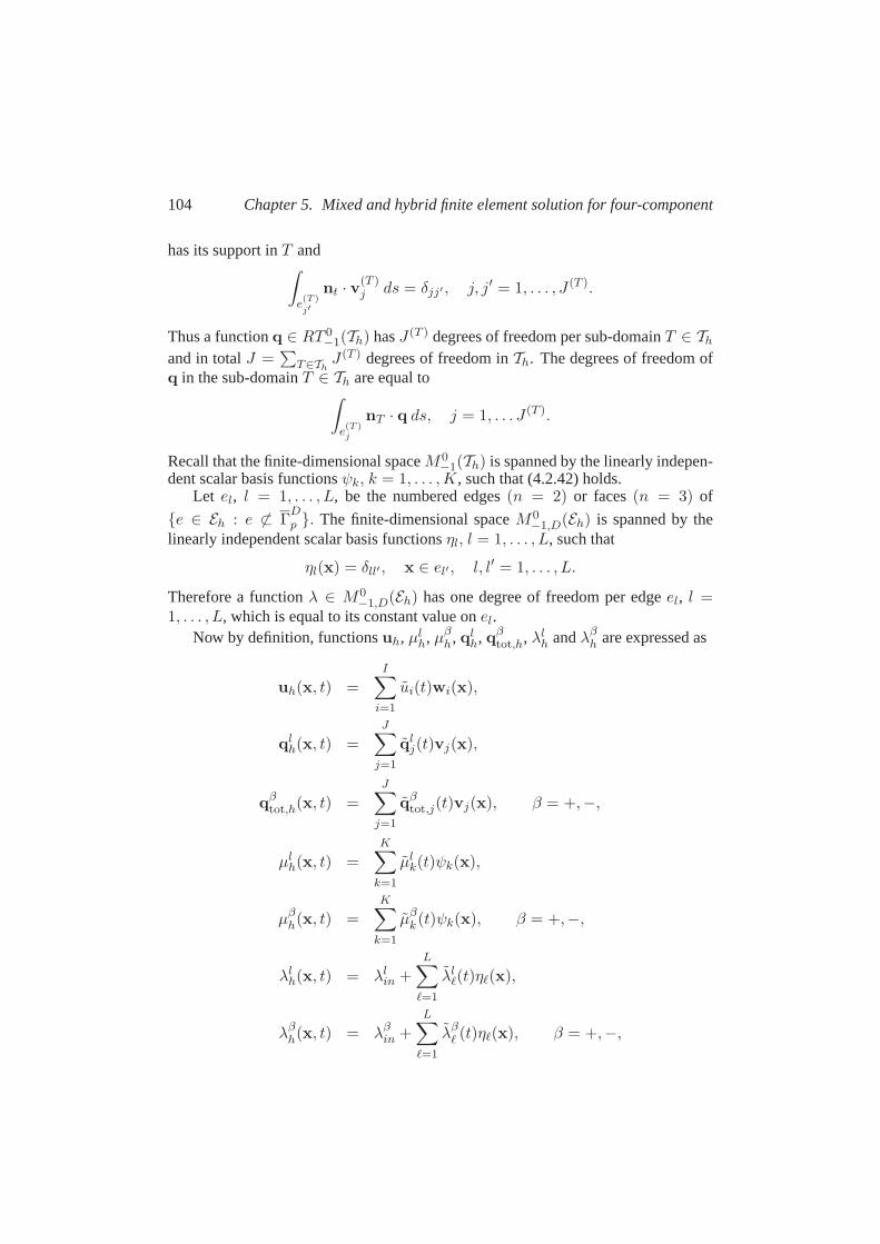
104 Chapter 5. Mixed and hybrid finite element solution for four-component
has its support inT and∫
e(T )
j′
nt · v(T )j ds = δjj′ , j, j′ = 1, . . . , J (T ).
Thus a functionq ∈ RT 0−1(Th) hasJ (T ) degrees of freedom per sub-domainT ∈ Th
and in totalJ =∑
T∈ThJ (T ) degrees of freedom inTh. The degrees of freedom of
q in the sub-domainT ∈ Th are equal to∫
e(T )j
nT · q ds, j = 1, . . . J (T ).
Recall that the finite-dimensional spaceM0−1(Th) is spanned by the linearly indepen-
dent scalar basis functionsψk, k = 1, . . . ,K, such that (4.2.42) holds.Let el, l = 1, . . . , L, be the numbered edges(n = 2) or faces(n = 3) of
e ∈ Eh : e 6⊂ ΓDp . The finite-dimensional spaceM0
−1,D(Eh) is spanned by thelinearly independent scalar basis functionsηl, l = 1, . . . , L, such that
ηl(x) = δll′ , x ∈ el′ , l, l′ = 1, . . . , L.
Therefore a functionλ ∈ M0−1,D(Eh) has one degree of freedom per edgeel, l =
1, . . . , L, which is equal to its constant value onel.Now by definition, functionsuh, µl
h, µβh, ql
h, qβtot,h, λl
h andλβh are expressed as
uh(x, t) =I∑
i=1
ui(t)wi(x),
qlh(x, t) =
J∑
j=1
qlj(t)vj(x),
qβtot,h(x, t) =
J∑
j=1
qβtot,j(t)vj(x), β = +,−,
µlh(x, t) =
K∑
k=1
µlk(t)ψk(x),
µβh(x, t) =
K∑
k=1
µβk(t)ψk(x), β = +,−,
λlh(x, t) = λl
in +L∑
ℓ=1
λlℓ(t)ηℓ(x),
λβh(x, t) = λβ
in +L∑
ℓ=1
λβℓ (t)ηℓ(x), β = +,−,
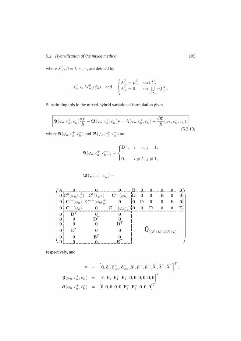
5.2. Hybridization of the mixed method 105
whereλβin, β = l,+,−, are defined by
λβin ∈M0
−1(Eh) and
λβ
in = µβin onΓD
p ,
λβin = 0 on
⋃e∈Eh
e\ΓDp .
Substituting this in the mixed-hybrid variational formulation gives
A(ϕh, c+h , c
−h )dy
dt+ B(ϕh, c
+h , c
−h )y = F(ϕh, c
+h , c
−h ) +
dG
dt(ϕh, c
+h , c
−h ),
(5.2.10)whereA(ϕh, c
+h , c
−h ) andB(ϕh, c
+h , c
−h ) are
A(ϕh, c+h , c
−h )ij =
BT , i = 5, j = 1,
0, i 6= 5, j 6= 1,
B(ϕh, c+h , c
−h ) =
A 0 0 0 B 0 0 0 0 0
0 Cll(ϕh/cβh) Cl+(ϕh) Cl−(ϕh) D 0 0 E 0 0
0 Cl+(ϕh) C++(ϕhc+h ) 0 0 D 0 0 E 0
0 Cl−(ϕh) 0 C−−(ϕhc−h ) 0 0 D 0 0 E
0 DT 0 00 0 DT 00 0 0 DT
0 ET 0 0 03(K+L)×3(K+L)
0 0 ET 00 0 0 ET
respectively, and
y =[u, ql, q+
tot, q−tot, µ
l, µ+, µ−, λl, λ
+, λ
−]T,
F(ϕh, c+h , c
−h ) =
[F,Fl
1,F+1 ,F
−1 ,0,0,0,0,0,0
]T
G(ϕh, c+h , c
−h ) =
[0,0,0,0,0,F+
2 ,F−2 ,0,0,0
]T.
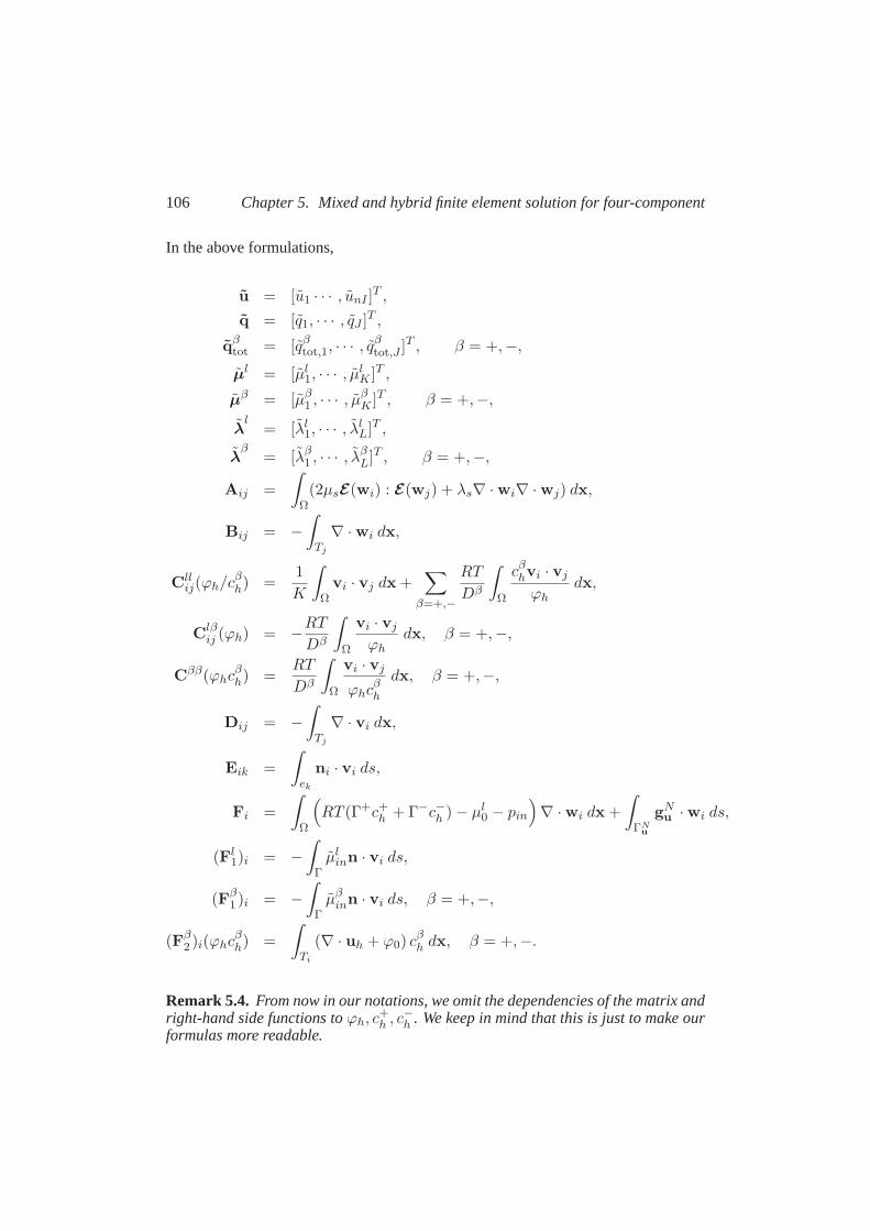
106 Chapter 5. Mixed and hybrid finite element solution for four-component
In the above formulations,
u = [u1 · · · , unI ]T ,
q = [q1, · · · , qJ ]T ,
qβtot = [qβ
tot,1, · · · , qβtot,J ]T , β = +,−,
µl = [µl1, · · · , µ
lK ]T ,
µβ = [µβ1 , · · · , µ
βK ]T , β = +,−,
λl
= [λl1, · · · , λ
lL]T ,
λβ
= [λβ1 , · · · , λ
βL]T , β = +,−,
Aij =
∫
Ω(2µsE(wi) : E(wj) + λs∇ · wi∇ · wj) dx,
Bij = −
∫
Tj
∇ · wi dx,
Cllij(ϕh/c
βh) =
1
K
∫
Ωvi · vj dx +
∑
β=+,−
RT
Dβ
∫
Ω
cβhvi · vj
ϕhdx,
Clβij (ϕh) = −
RT
Dβ
∫
Ω
vi · vj
ϕhdx, β = +,−,
Cββ(ϕhcβh) =
RT
Dβ
∫
Ω
vi · vj
ϕhcβh
dx, β = +,−,
Dij = −
∫
Tj
∇ · vi dx,
Eik =
∫
ek
ni · vi ds,
Fi =
∫
Ω
(RT (Γ+c+h + Γ−c−h ) − µl
0 − pin
)∇ · wi dx +
∫
ΓNu
gNu · wi ds,
(Fl1)i = −
∫
Γµl
inn · vi ds,
(Fβ1 )i = −
∫
Γµβ
inn · vi ds, β = +,−,
(Fβ2 )i(ϕhc
βh) =
∫
Ti
(∇ · uh + ϕ0) cβh dx, β = +,−.
Remark 5.4. From now in our notations, we omit the dependencies of the matrix andright-hand side functions toϕh, c
+h , c
−h . We keep in mind that this is just to make our
formulas more readable.
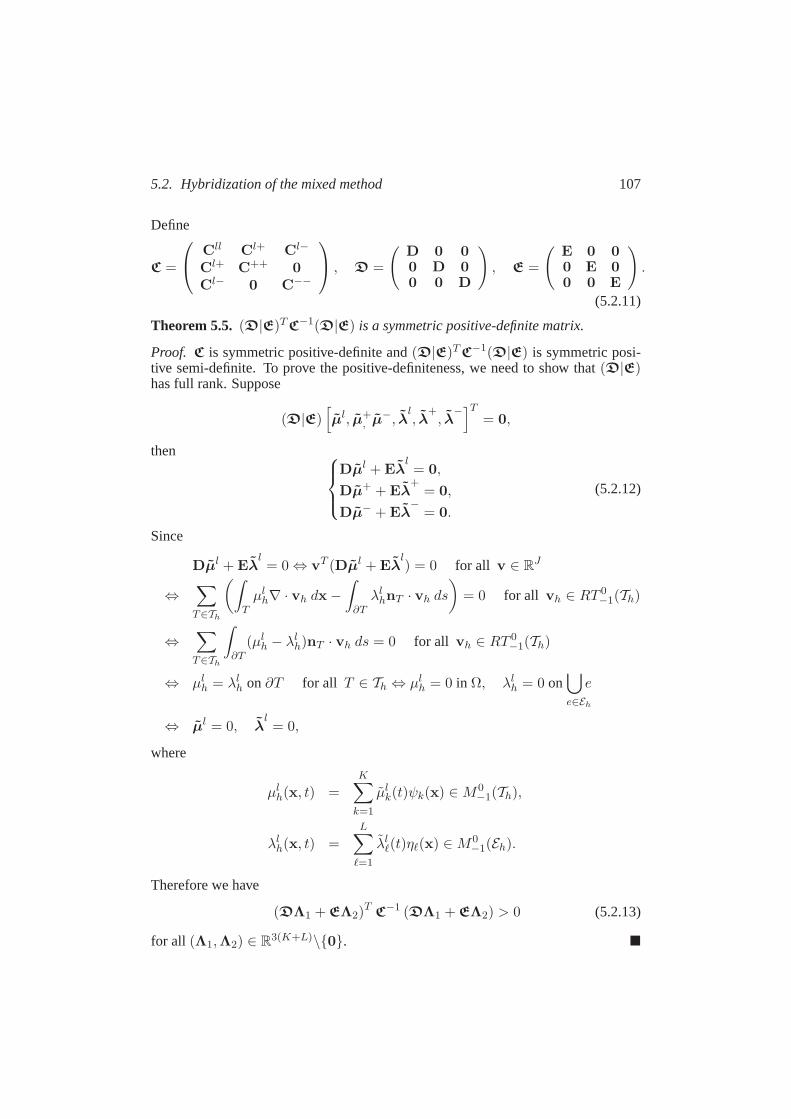
5.2. Hybridization of the mixed method 107
Define
C =
Cll Cl+ Cl−
Cl+ C++ 0
Cl− 0 C−−
, D =
(D 0 00 D 00 0 D
), E =
(E 0 00 E 00 0 E
).
(5.2.11)
Theorem 5.5. (D|E)T C−1(D|E) is a symmetric positive-definite matrix.
Proof. C is symmetric positive-definite and(D|E)T C−1(D|E) is symmetric posi-tive semi-definite. To prove the positive-definiteness, we need to show that (D|E)has full rank. Suppose
(D|E)[µl, µ+
, µ−, λl, λ
+, λ
−]T
= 0,
then
Dµl + Eλl= 0,
Dµ+ + Eλ+
= 0,
Dµ− + Eλ−
= 0.
(5.2.12)
Since
Dµl + Eλl= 0 ⇔ vT (Dµl + Eλ
l) = 0 for all v ∈ R
J
⇔∑
T∈Th
(∫
Tµl
h∇ · vh dx −
∫
∂Tλl
hnT · vh ds
)= 0 for all vh ∈ RT 0
−1(Th)
⇔∑
T∈Th
∫
∂T(µl
h − λlh)nT · vh ds = 0 for all vh ∈ RT 0
−1(Th)
⇔ µlh = λl
h on∂T for all T ∈ Th ⇔ µlh = 0 in Ω, λl
h = 0 on⋃e
e∈Eh
⇔ µl = 0, λl= 0,
where
µlh(x, t) =
K∑
k=1
µlk(t)ψk(x) ∈M0
−1(Th),
λlh(x, t) =
L∑
ℓ=1
λlℓ(t)ηℓ(x) ∈M0
−1(Eh).
Therefore we have
(DΛ1 + EΛ2)T
C−1 (DΛ1 + EΛ2) > 0 (5.2.13)
for all (Λ1,Λ2) ∈ R3(K+L)\0.
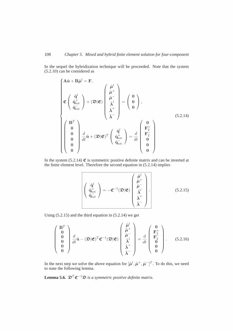
108 Chapter 5. Mixed and hybrid finite element solution for four-component
In the sequel the hybridization technique will be proceeded. Note that the system(5.2.10) can be considered as
Au + Bµl = F,
C
ql
q+tot
q−tot
+ (D|E)
µl
µ+
µ−
λl
λ+
λ−
=
0
0
0
,
BT
0
0
0
0
0
d
dtu + (D|E)T
ql
q+tot
q−tot
=
d
dt
0
F+2
F−2
0
0
0
(5.2.14)
In the system (5.2.14)C is symmetric positive definite matrix and can be inverted atthe finite element level. Therefore the second equation in (5.2.14) implies
ql
q+tot
q−tot
= −C−1(D|E)
µl
µ+
µ−
λl
λ+
λ−
. (5.2.15)
Using (5.2.15) and the third equation in (5.2.14) we get
BT
00000
d
dtu − (D|E)T C−1(D|E)
µl
µ+
µ−
λl
λ+
λ−
=d
dt
0
F+2
F−2000
. (5.2.16)
In the next step we solve the above equation for[µl, µ+, µ−]T . To do this, we needto state the following lemma.
Lemma 5.6. DT C−1D is a symmetric positive definite matrix.
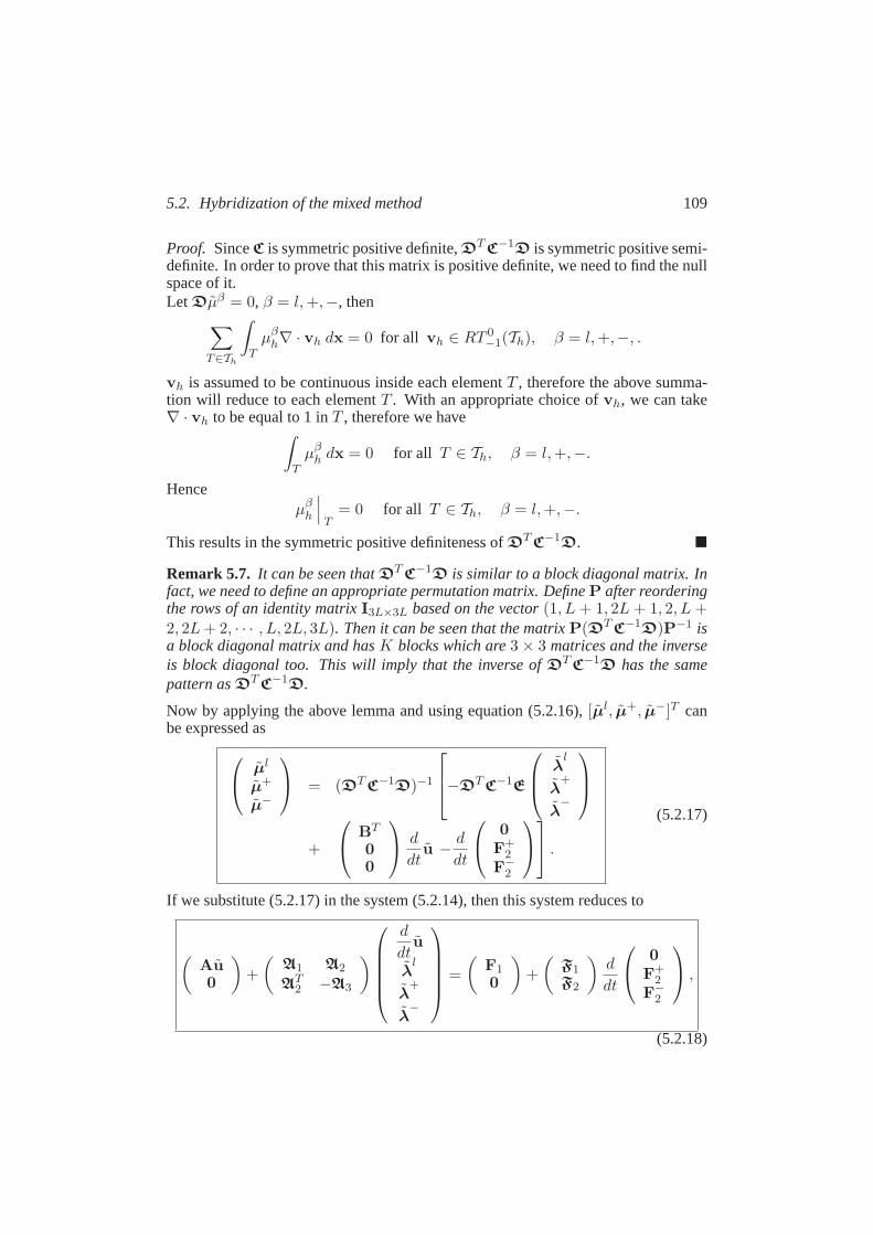
5.2. Hybridization of the mixed method 109
Proof. SinceC is symmetric positive definite,DT C−1D is symmetric positive semi-definite. In order to prove that this matrix is positive definite, we need to find the nullspace of it.Let Dµβ = 0, β = l,+,−, then
∑
T∈Th
∫
Tµβ
h∇ · vh dx = 0 for all vh ∈ RT 0−1(Th), β = l,+,−, .
vh is assumed to be continuous inside each elementT , therefore the above summa-tion will reduce to each elementT . With an appropriate choice ofvh, we can take∇ · vh to be equal to 1 inT , therefore we have
∫
Tµβ
h dx = 0 for all T ∈ Th, β = l,+,−.
Henceµβ
h
T
= 0 for all T ∈ Th, β = l,+,−.
This results in the symmetric positive definiteness ofDT C−1D.
Remark 5.7. It can be seen thatDT C−1D is similar to a block diagonal matrix. Infact, we need to define an appropriate permutation matrix. DefineP after reorderingthe rows of an identity matrixI3L×3L based on the vector(1, L + 1, 2L + 1, 2, L +2, 2L+ 2, · · · , L, 2L, 3L). Then it can be seen that the matrixP(DT C−1D)P−1 isa block diagonal matrix and hasK blocks which are3 × 3 matrices and the inverseis block diagonal too. This will imply that the inverse ofDT C−1D has the samepattern asDT C−1D.
Now by applying the above lemma and using equation (5.2.16),[µl, µ+, µ−]T canbe expressed as
µl
µ+
µ−
= (DT C−1D)−1
−DT C−1E
λl
λ+
λ−
+
BT
00
d
dtu −
d
dt
0
F+2
F−2
.
(5.2.17)
If we substitute (5.2.17) in the system (5.2.14), then this system reduces to
(Au0
)+
(A1 A2
AT2 −A3
)
d
dtu
λl
λ+
λ−
=
(F1
0
)+
(F1F2
)d
dt
0
F+2
F−2
,
(5.2.18)
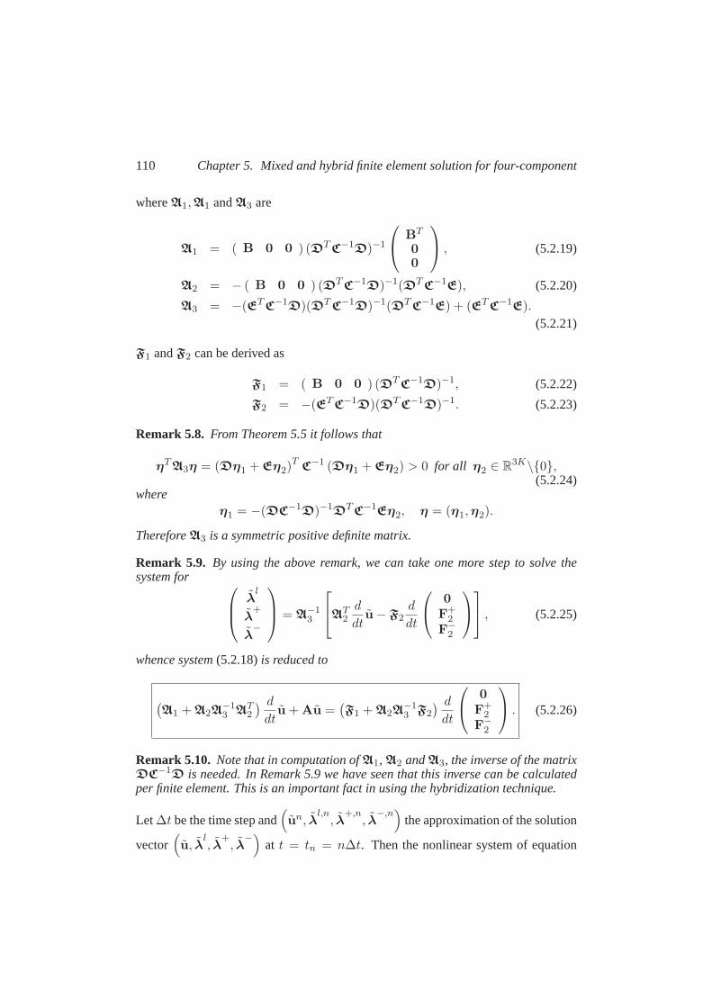
110 Chapter 5. Mixed and hybrid finite element solution for four-component
whereA1,A1 andA3 are
A1 = ( B 0 0 ) (DT C−1D)−1
BT
00
, (5.2.19)
A2 = − ( B 0 0 ) (DT C−1D)−1(DT C−1E), (5.2.20)
A3 = −(ET C−1D)(DT C−1D)−1(DT C−1E) + (ET C−1E).
(5.2.21)
F1 andF2 can be derived as
F1 = ( B 0 0 ) (DT C−1D)−1, (5.2.22)
F2 = −(ET C−1D)(DT C−1D)−1. (5.2.23)
Remark 5.8. From Theorem 5.5 it follows that
ηT A3η = (Dη1 + Eη2)T
C−1 (Dη1 + Eη2) > 0 for all η2 ∈ R3K\0,
(5.2.24)where
η1 = −(DC−1D)−1DT C−1Eη2, η = (η1,η2).
ThereforeA3 is a symmetric positive definite matrix.
Remark 5.9. By using the above remark, we can take one more step to solve thesystem for
λ
l
λ+
λ−
= A
−13
AT
2
d
dtu − F2
d
dt
0
F+2
F−2
, (5.2.25)
whence system(5.2.18)is reduced to
(A1 + A2A
−13 AT
2
) ddt
u + Au =(F1 + A2A
−13 F2
) ddt
0
F+2
F−2
. (5.2.26)
Remark 5.10. Note that in computation ofA1, A2 andA3, the inverse of the matrixDC−1D is needed. In Remark 5.9 we have seen that this inverse can be calculatedper finite element. This is an important fact in using the hybridization technique.
Let ∆t be the time step and(un, λ
l,n, λ
+,n, λ
−,n)
the approximation of the solution
vector(u, λ
l, λ
+, λ
−)
at t = tn = n∆t. Then the nonlinear system of equation
5.3. Numerical simulations 111
(5.2.18) resulting from backward Euler is:
(Aun+1
0
)+
A1
(ϕn+1
h , c+,n+1h , c−,n+1
h
)A2
(ϕn+1
h , c+,n+1h , c−,n+1
h
)
AT2
(ϕn+1
h , c+,n+1h , c−,n+1
h
)−A3
(ϕn+1
h , c+,n+1h , c−,n+1
h
)
×
un+1 − un
∆tλ
l,n+1
λ+,n+1
λ−,n+1
=
(F1
0
)+
F1
(ϕn+1
h , c+,n+1h , c−,n+1
h
)
F2
(ϕn+1
h , c+,n+1h , c−,n+1
h
)
×
0
F+2
(ϕn+1
h , c+,n+1h , c−,n+1
h
)− F+
2
(ϕn
h, c+,nh , c−,n
h
)
∆tF−
2
(ϕn+1
h , c+,n+1h , c−,n+1
h
)− F−
2
(ϕn
h, c+,nh , c−,n
h
)
∆t
. (5.2.27)
The assumption thatcβh, β = +,−, andϕh are known transforms the system into a
linear one. Forϕh the value at the old time step is taken. Thus the value ofcfch at the
old time level is known and therefore the differencec+h − c−h by electro-neutrality.
Definec± = c+ + c−, then the solutionµβh from (5.2.17) and (5.2.27) for fixedcβh,
β = +,−, can be denoted symbolically by(µ+h , µ
−h ) = A−1(c±h )b(c±h ), whereA
andb represent the matrix and right-hand side of the linear system. Nowc±h canbe computed by the third relation in the secondary equations in (2.7.7), i.e.,c±h =
f(µ+h , µ
−h , c
±h ). Ergo, we obtain the non-linear system
c±h = f(A−1(c±h )b(c±h ), c±h
). (5.2.28)
This system can be solved by an iterative procedure for non-linear system (see Algo-rithm 1).
In each iteration a linear system has to be solved. It should be observed thatdifferent scales are apparent in (5.2.18) that will result in a poorly scaled matrix inthe linear system. Therefore the matrixA is replaced by the scaled matrixDAD,where the diagonal matrixD is defined by
D2 = diag
(L
∆t(2µs + λs),L
K,
RTL
D+ϕ0cfc0
,RTL
D−ϕ0cfc0
). (5.2.29)
HereL is a representative length scale.
5.3 Numerical simulations
In this section the element contributions to the matrices and right-hand sides in(5.2.18) are computed.
112 Chapter 5. Mixed and hybrid finite element solution for four-component
Algorithm 1 Solving the nonlinear system (5.2.27) by using iterations
Givenϕnh, c±,n
h and givenǫcriteria⇐ 1while criteria> ǫ do
cfc,nh ⇐ cfc
0 exp
(−
ϕnh − ϕ0
ϕ0(1 − ϕ0)
)
d±,nh ⇐ c+,n
h − c−,nh = cfc,n
h by electroneutralityc+,nh ⇐ (c±,n
h + d±,nh )/2
c−,nh ⇐ c±,n
h − c+,nh(
un+1, λl,n+1
, λ+,n+1
, λ−,n+1
)⇐ solve thelinear system (5.2.27)
(µl,n+1, µ+,n+1, µ−,n+1
)⇐ use equation (5.2.17)
(ϕn+1h , c+,n+1
h , c−,n+1h ) ⇐ use the secondary equations in (2.7.7)
criteria⇐ minβ=+,− ‖cβ,n+1h − cβ,n
h ‖0
cβ,nh ⇐ cβ,n+1
h , β = +,−
ϕnh ⇐ ϕn+1
hend whilecβ,n+1h ⇐ cβ,n+1
h
ϕn+1h ⇐ ϕn+1
h
The element contribution to the elasticity matrixA andB in (5.2.18) can becomputed in an standard way. For element contribution to the matricesCβγ , β, γ =l,+,−, recall (4.4.4)
(C
(T )
J(T )×J(T )
)
ij=
n∑
k=1
c(T )kk (Akk)ij +
n∑
k=1
n−1∑
l=1
c(T )kl (Akl + Alk)ij ,
where all matrices in the summations are symmetric are given in (Kaasschieter andHuijben, 1992).
As an example we takeT to be a parallelogram, wheren = 2 andJ (T ) = 4, thuswe have
A11 =1
6
2 0 −1 00 0 0 0−1 0 2 00 0 0 0
, A12 +A21 =
1
4
0 1 0 −11 0 −1 00 −1 0 1−1 0 1 0
,
A22 =1
6
0 0 0 00 2 0 −10 0 0 00 −1 0 2
.
5.3. Numerical simulations 113
Another example is a triangle wheren = 2 andJ (T ) = 3,
A11 =1
12
(1 −1 1−1 3 −11 −1 1
), A12 +A21 =
1
12
(1 −1 −1−1 −3 3−1 3 −3
),
A22 =1
12
(1 1 −11 1 −1−1 −1 3
).
Using Green’s formula, (4.2.30) and (4.2.35), simple formulas can be derived forthe element contributions of the remaining matrices and right hand sides in (5.2.18),namely
(D
(T )
J(T )×1
)
i= −
∫
T∇ · v
(T )i dx = −1, (5.3.1)
(G
(T )
J(T )×J(T )
)
ik=
∫
e(T )k
nT · v(T )i ds = δik, (5.3.2)
F β1 =
−µin, if ei ⊂ ΓD
p
0 otherwise., β = l,+,−. (5.3.3)
The computation of(DT C−1D)−1 is essential when determining the matricesAi,(i = 1, 2, 3) in (5.2.19) - (5.2.21). This matrix is a block diagonal matrix (Remark5.9) and it can thus be computed at the finite element level. The matricesAi areobtained by assembling their element contributions. The right-hand side vectors F1andF2 can be computed in an analogous way.
5.3.1 Confined consolidation and free swelling
In this section, numerical solutions are calculated for confined consolidation and freeswelling. To verify the method, solutions are compared with the analytical solutionsfrom chapter 3.
The homogeneous sample is placed frictionless in a holder. Figure 5.1 illustratesthe experimental setup. At the bottomy = 0, the sample is in contact with a glassfilter saturated by a sodium chloride solution. An impermeable piston is placed onthetop of the sample,y = L, where an external mechanical load is applied. The samplewas made out of a hydrogel. A bathing solution flowed through a porous glass filterat the bottom of the sample.
Consolidation
In the consolidation experiment, we apply a load on the piston to be equal tof(t) =−f0H(t − t0), with H(t − t0) the Heaviside function andf0 > 0. The externalconcentration is kept constant during the test.
For the reference values for the electro-chemical potentials we choose
µl0 = 2RTcout, µβ
0 = −RT lncout
c. (5.3.4)

114 Chapter 5. Mixed and hybrid finite element solution for four-component
piston
confiningring
sample
fluid channel
glass filter+
+
+
+
+
++++
++
F
L
oil film
Figure 5.1.Schematic representation of the experimental set-up
By Donnan equilibrium, we know that the electro-chemical potentials are continuousat the boundary, i.e.,µβ
in = µβout, β = l,+,−, where subscripts ‘in’ and ‘out’ stand
for inner and outer solution, respectively.Assume
Γ+in = Γ−
in = Γ, Γ+out = Γ−
out = 1, pout = 0, ξout = 0,
then
µlin = µl
out
= µl0 + pout − 2RTΓoutcout = 0,
µβin = µβ
out
= µβout + zβFξout +RTΓout ln
cout
c= 0, β = +,−.
Therefore, the initial and boundary conditions for the displacement and electro-chemicalpotentials with respect to the steady reference statet = t0 are:
[µl µ+ µ−
](0, t) = [ 0 0 0 ] ,
[µl µ+ µ−
](y, t0) =
[µl
t0 µ+t0
µ−t0],
u(0, t) = 0,
u(y, t0) = 0, (5.3.5)
where[µl
t0 µ+t0
µ−t0]
= [ f0 0 0 ].
Free Swelling
In free swelling experiment, initially the tissue sample is at equilibrium with theexternal bathing solution with concentrationcout(t
−0 ). At t = t+0 , the concentration
5.3. Numerical simulations 115
of the external solution at the bottom of sample decreases tocout(t+0 ) instantaneously.
This lowering of the concentration causes the tissue to swell to a new equilibriumstate.For the reference values of electro-chemical potentials we choose
µl0 = 2RTcout, µβ
0 = −RT lncout
c. (5.3.6)
The initial and boundary conditions for the displacement and electro-chemical poten-tials with respect to the steady reference statet = t0 are:
[µl µ+ µ−
](0, t) =
[µl
in µ+in µ−in
],
[µl µ+ µ−
](y, t0) =
[µl
t0 µ+t0
µ−t0],
u(0, t) = 0,
u(y, t0) = 0, (5.3.7)
in whichµβt0
= 0, β = l,+,−, and
µlin = −2RT∆cout,
µ+in = RT ln
cout(t+0 )
cout(t−0 ),
µ−in = RT lncout(t
+0 )
cout(t−0 ),
(5.3.8)
∆cout = cout(t+0 ) − cout(t
−0 ) wheret+0 andt−0 are the time just after and beforet0
when chemical loading is applied.
Results
Parameter Unit Value2µs + λs MPa 4 × 10³
K m4 N−1 s−1 1.0 × 10⁻¹⁸
cfc mol m−3−2 × 10²
cout mol m−3 1 × 10²
ϕ 0.1D+ m2 s−1 13.3 × 10⁻¹⁰
D− m2 s−1 20.3 × 10⁻¹⁰
R J mol−1 K−1 8.3145T K 293F C mol−1 96484.6Γ 0.9
In this section, the results for the confinedconsolidation and the free swelling areprescribed. For both computations, theparameters in the table are taken. Thesetwo experiments are taken from (Frijns,2001) and our aim is to validate the nu-merical solutions by analytical solutionsdescribed in chapter 3.
As mentioned in the previous section,an uniaxial confined swelling and com-pression experiment is performed on acylindrical sample of cartilage substitute.This sample, with the diameter of 4 mmand the height of approximately 1 mm isput in an insulating conforming ring. A piston on the top of the sample is loaded me-chanically. A bathing solution flows through a porous glass filter at the bottomof the
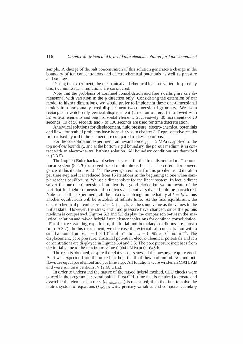
116 Chapter 5. Mixed and hybrid finite element solution for four-component
sample. A change of the salt concentration of this solution generates a change in theboundary of ion concentrations and electro-chemical potentials as well aspressureand voltage.
During the experiment, the mechanical and chemical load are varied. Inspired bythis, two numerical simulations are considered.
Note that the problems of confined consolidation and free swelling are one di-mensional with variation in they direction only. Considering the extension of ourmodel to higher dimensions, we would prefer to implement these one-dimensionalmodels in a horizontally-fixed displacement two-dimensional geometry. We usearectangle in which only vertical displacement (direction of force) is allowedwith32 vertical elements and one horizontal element. Successively, 30 increments of 20seconds, 10 of 50 seconds and 7 of 100 seconds are used for time discretisation.
Analytical solutions for displacement, fluid pressure, electro-chemical potentialsand flows for both of problems have been derived in chapter 3. Representative resultsfrom mixed hybrid finite element are compared to these solutions.
For the consolidation experiment, an inward forcef0 = 5 MPa is applied to thetop no-flow boundary, and at the bottom rigid boundary, the porous medium is in con-tact with an electro-neutral bathing solution. All boundary conditions are describedin (5.3.5).
The implicit Euler backward scheme is used for the time discretisation. The non-linear system (5.2.26) is solved based on iterations forc±. The criteria for conver-gence of this iteration is10−12. The average iterations for this problem is 10 iterationper time step and it is reduced from 15 iterations in the beginning to one when sam-ple reaches equilibrium. We use a direct solver for the linear system. In fact, a directsolver for our one-dimensional problem is a good choice but we are aware of thefact that for higher-dimensional problems an iterative solver should be considered.Note that in this experiment, all the unknowns change immediately att = t0 s, thusanother equilibrium will be establish at infinite time. At the final equilibrium, theelectro-chemical potentialsµβ , β = l,+,−, have the same value as the values in theinitial state. However, the stress and fluid pressure have changed, since the porousmedium is compressed, Figures 5.2 and 5.3 display the comparison between theana-lytical solution and mixed hybrid finite element solutions for confined consolidation.
For the free swelling experiment, the initial and boundary conditions are chosenfrom (5.3.7). In this experiment, we decrease the external salt concentration with asmall amount fromcout = 1 × 10² mol m−3 to cout = 0.995 × 10² mol m−3. Thedisplacement, pore pressure, electrical potential, electro-chemical potentials and ionconcentrations are displayed in Figures 5.4 and 5.5. The pore pressureincreases fromthe initial value to the maximum value0.0041 MPa at0.1648 h.
The results obtained, despite the relative coarseness of the meshes are quite good.As it was expected from the mixed method, the fluid flow and ion inflows and out-flows are equal per element and per time step. All functions were written in MATLABand were run on a pentium IV (2.66 GHz).
In order to understand the nature of the mixed hybrid method, CPU checks wereplaced in the program at several points. First CPU time that is required to create andassemble the element matrices (telem,assem) is measured; then the time to solve thematrix system of equations (tsolve); write primary variables and compute secondary
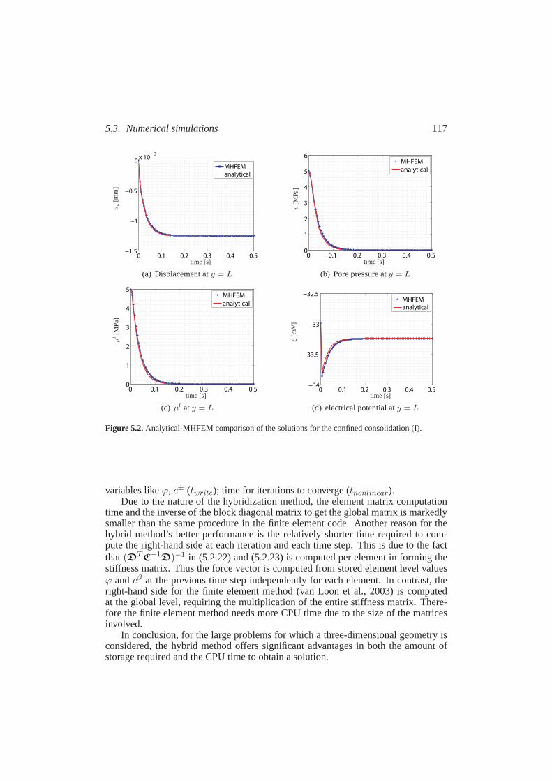
5.3. Numerical simulations 117
0 0.1 0.2 0.3 0.4 0.5−1.5
−1
−0.5
0x 10
−3
MHFEM
analytical
time [s]
uy
[mm
]
(a) Displacement aty = L
0 0.1 0.2 0.3 0.4 0.50
1
2
3
4
5
6
MHFEM
analytical
time [s]
p[M
Pa]
(b) Pore pressure aty = L
0 0.1 0.2 0.3 0.4 0.50
1
2
3
4
5
MHFEM
analytical
time [s]
µl[M
Pa]
(c) µl aty = L
0 0.1 0.2 0.3 0.4 0.5−34
−33.5
−33
−32.5
MHFEM
analytical
time [s]
ξ[m
V]
(d) electrical potential aty = L
Figure 5.2.Analytical-MHFEM comparison of the solutions for the confined consolidation (I).
variables likeϕ, c± (twrite); time for iterations to converge (tnonlinear).Due to the nature of the hybridization method, the element matrix computation
time and the inverse of the block diagonal matrix to get the global matrix is markedlysmaller than the same procedure in the finite element code. Another reason for thehybrid method’s better performance is the relatively shorter time required to com-pute the right-hand side at each iteration and each time step. This is due to the factthat(DT C−1D)−1 in (5.2.22) and (5.2.23) is computed per element in forming thestiffness matrix. Thus the force vector is computed from stored element level valuesϕ andcβ at the previous time step independently for each element. In contrast, theright-hand side for the finite element method (van Loon et al., 2003) is computedat the global level, requiring the multiplication of the entire stiffness matrix. There-fore the finite element method needs more CPU time due to the size of the matricesinvolved.
In conclusion, for the large problems for which a three-dimensional geometry isconsidered, the hybrid method offers significant advantages in both the amount ofstorage required and the CPU time to obtain a solution.
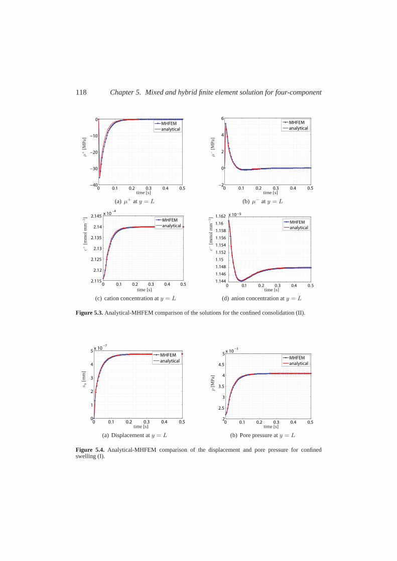
118 Chapter 5. Mixed and hybrid finite element solution for four-component
0 0.1 0.2 0.3 0.4 0.5−40
−30
−20
−10
0
MHFEM
analytical
time [s]
µ+
[MP
a]
(a) µ+ aty = L
0 0.1 0.2 0.3 0.4 0.5−2
0
2
4
6
MHFEM
analytical
time [s]
µ−
[MP
a]
(b) µ− aty = L
0 0.1 0.2 0.3 0.4 0.52.115
2.12
2.125
2.13
2.135
2.14
2.145x 10
−4
MHFEM
analytical
time [s]
c+[m
mol
mm
−3]
(c) cation concentration aty = L
0 0.1 0.2 0.3 0.4 0.51.144
1.146
1.148
1.15
1.152
1.154
1.156
1.158
1.16
1.162 x 10 −5
MHFEM
analytical
time [s]
c−[m
mol
mm
−3]
(d) anion concentration aty = L
Figure 5.3.Analytical-MHFEM comparison of the solutions for the confined consolidation (II).
0 0.1 0.2 0.3 0.4 0.50
1
2
3
4
5x 10
−7
MHFEM
analytical
time [s]
uy
[mm
]
(a) Displacement aty = L
0 0.1 0.2 0.3 0.4 0.52
2.5
3
3.5
4
4.5
5x 10
−3
MHFEM
analytical
time [s]
p[M
Pa]
(b) Pore pressure aty = L
Figure 5.4. Analytical-MHFEM comparison of the displacement and pore pressure for confinedswelling (I).
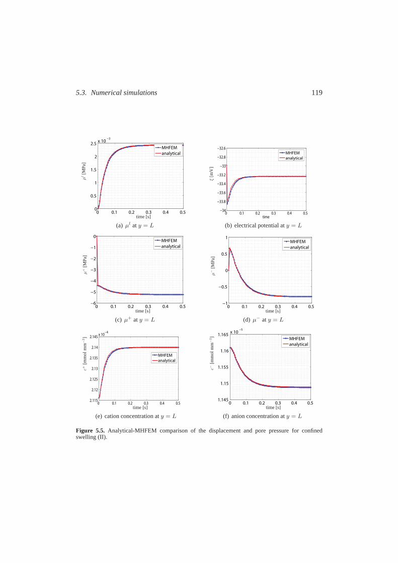
5.3. Numerical simulations 119
0 0.1 0.2 0.3 0.4 0.50
0.5
1
1.5
2
2.5x 10
−3
MHFEM
analytical
time [s]
µl[M
Pa]
(a) µl aty = L
0 0.1 0.2 0.3 0.4 0.5−34
−33.8
−33.6
−33.4
−33.2
−33
−32.8
−32.6
time
MHFEM
analytical
ξ[m
V]
(b) electrical potential aty = L
0 0.1 0.2 0.3 0.4 0.5−6
−5
−4
−3
−2
−1
0
MHFEM
analytical
time [s]
µ+
[MP
a]
(c) µ+ aty = L
0 0.1 0.2 0.3 0.4 0.5−1
−0.5
0
0.5
1
MHFEM
analytical
time [s]
µ−
[MP
a]
(d) µ− aty = L
0 0.1 0.2 0.3 0.4 0.52.115
2.12
2.125
2.13
2.135
2.14
2.145x 10
−4
MHFEM
analytical
time [s]
c+[m
mol
mm
−3]
(e) cation concentration aty = L
0 0.1 0.2 0.3 0.4 0.51.145
1.15
1.155
1.16
1.165x 10
−5
MHFEM
analytical
time [s]
c−[m
mol
mm
−3]
(f) anion concentration aty = L
Figure 5.5. Analytical-MHFEM comparison of the displacement and pore pressure for confinedswelling (II).
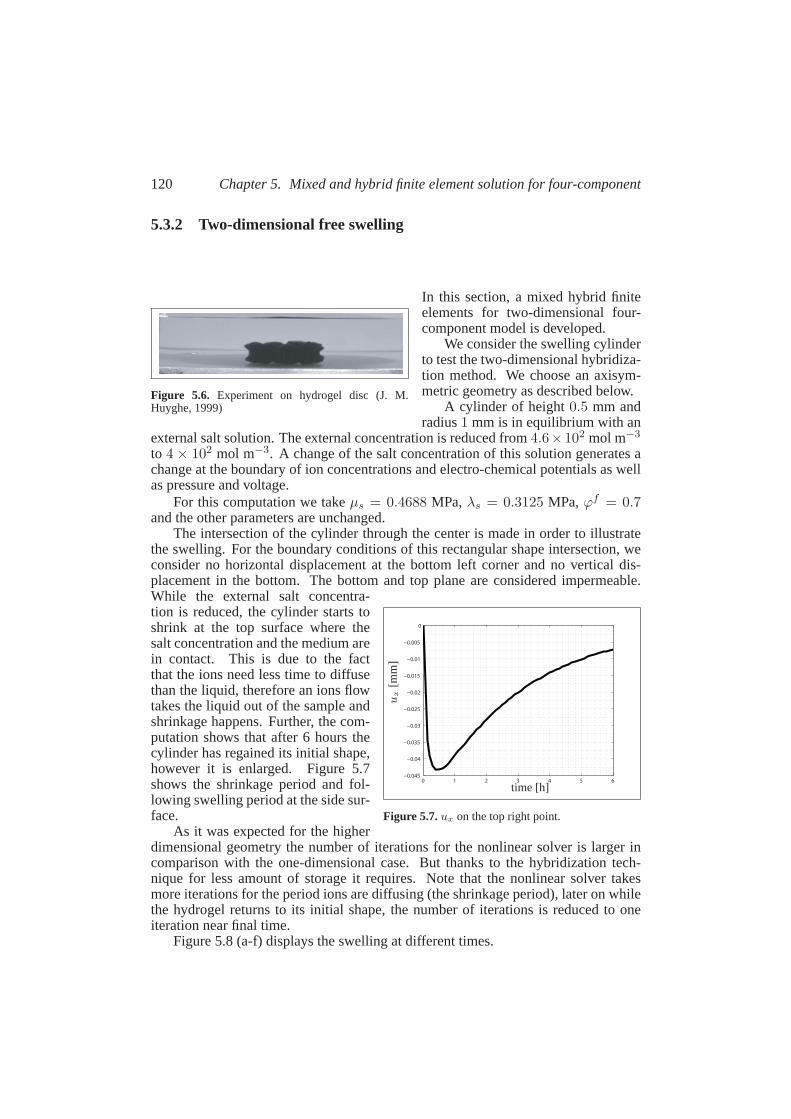
120 Chapter 5. Mixed and hybrid finite element solution for four-component
5.3.2 Two-dimensional free swelling
Figure 5.6. Experiment on hydrogel disc (J. M.Huyghe, 1999)
In this section, a mixed hybrid finiteelements for two-dimensional four-component model is developed.
We consider the swelling cylinderto test the two-dimensional hybridiza-tion method. We choose an axisym-metric geometry as described below.
A cylinder of height0.5 mm andradius1 mm is in equilibrium with an
external salt solution. The external concentration is reduced from4.6×102 mol m−3
to 4 × 10² mol m−3. A change of the salt concentration of this solution generates achange at the boundary of ion concentrations and electro-chemical potentials as wellas pressure and voltage.
For this computation we takeµs = 0.4688 MPa,λs = 0.3125 MPa,ϕf = 0.7and the other parameters are unchanged.
The intersection of the cylinder through the center is made in order to illustratethe swelling. For the boundary conditions of this rectangular shape intersection, weconsider no horizontal displacement at the bottom left corner and no vertical dis-placement in the bottom. The bottom and top plane are considered impermeable.
0 1 2 3 4 5 6−0.045
−0.04
−0.035
−0.03
−0.025
−0.02
−0.015
−0.01
−0.005
0
time [h]
ux
[mm
]
Figure 5.7.ux on the top right point.
While the external salt concentra-tion is reduced, the cylinder starts toshrink at the top surface where thesalt concentration and the medium arein contact. This is due to the factthat the ions need less time to diffusethan the liquid, therefore an ions flowtakes the liquid out of the sample andshrinkage happens. Further, the com-putation shows that after 6 hours thecylinder has regained its initial shape,however it is enlarged. Figure 5.7shows the shrinkage period and fol-lowing swelling period at the side sur-face.
As it was expected for the higherdimensional geometry the number of iterations for the nonlinear solver is larger incomparison with the one-dimensional case. But thanks to the hybridization tech-nique for less amount of storage it requires. Note that the nonlinear solver takesmore iterations for the period ions are diffusing (the shrinkage period), later on whilethe hydrogel returns to its initial shape, the number of iterations is reduced tooneiteration near final time.
Figure 5.8 (a-f) displays the swelling at different times.
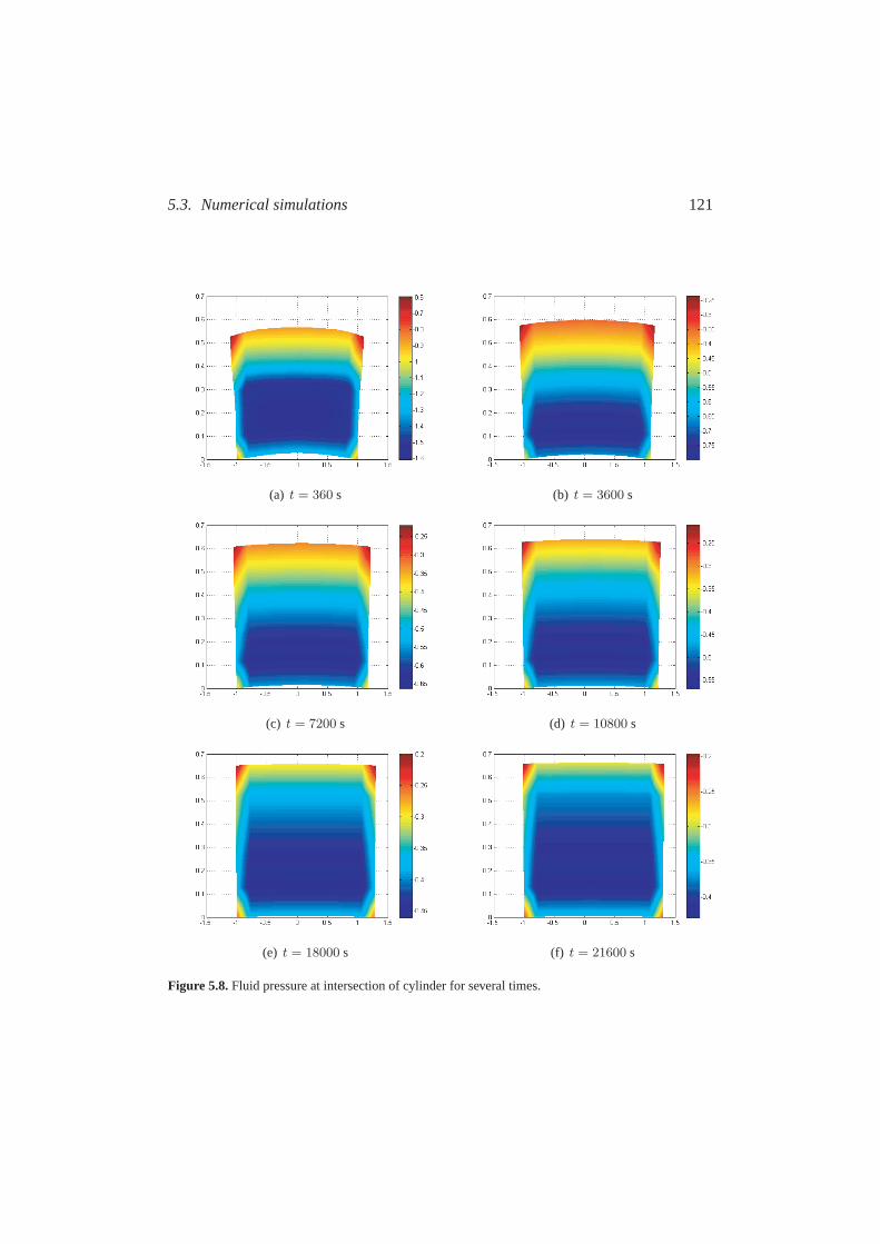
5.3. Numerical simulations 121
(a) t = 360 s (b) t = 3600 s
(c) t = 7200 s (d) t = 10800 s
(e) t = 18000 s (f) t = 21600 s
Figure 5.8.Fluid pressure at intersection of cylinder for several times.
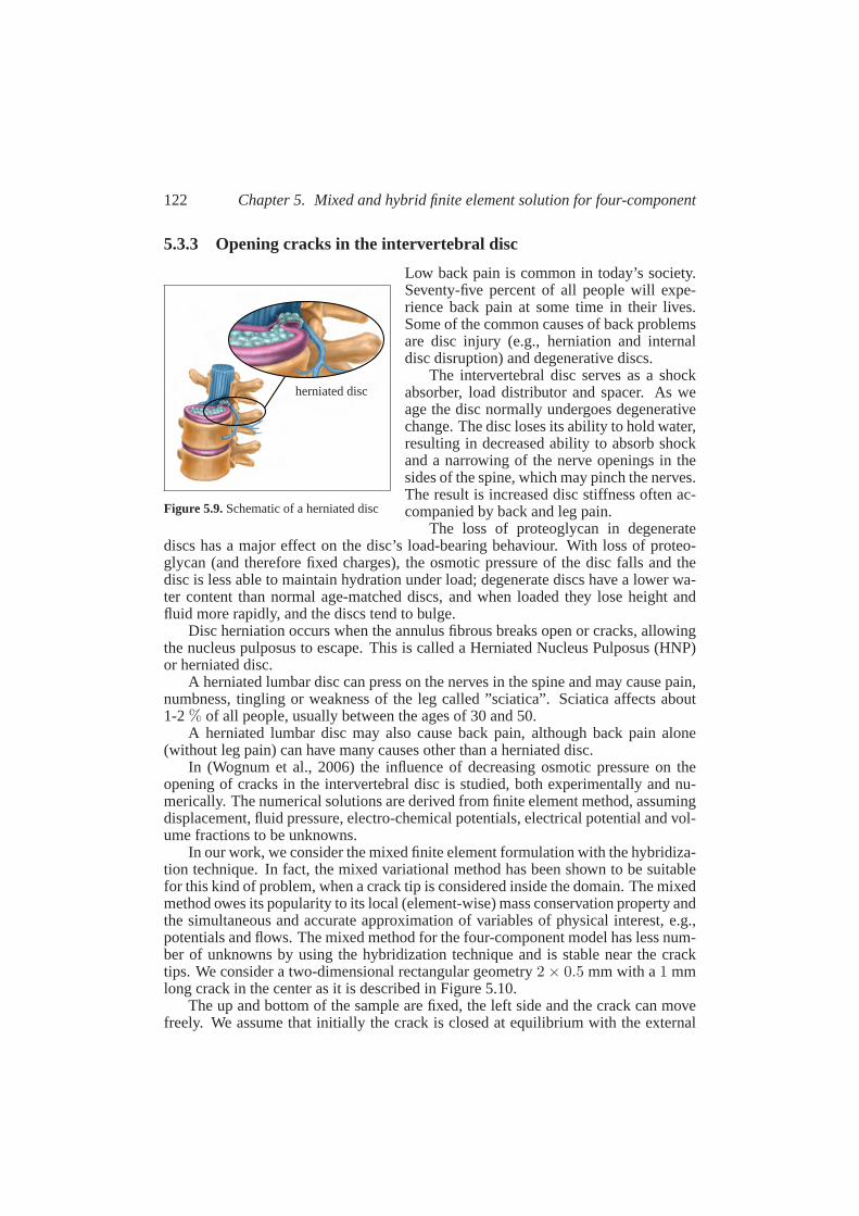
122 Chapter 5. Mixed and hybrid finite element solution for four-component
5.3.3 Opening cracks in the intervertebral disc
herniated disc
Figure 5.9.Schematic of a herniated disc
Low back pain is common in today’s society.Seventy-five percent of all people will expe-rience back pain at some time in their lives.Some of the common causes of back problemsare disc injury (e.g., herniation and internaldisc disruption) and degenerative discs.
The intervertebral disc serves as a shockabsorber, load distributor and spacer. As weage the disc normally undergoes degenerativechange. The disc loses its ability to hold water,resulting in decreased ability to absorb shockand a narrowing of the nerve openings in thesides of the spine, which may pinch the nerves.The result is increased disc stiffness often ac-companied by back and leg pain.
The loss of proteoglycan in degeneratediscs has a major effect on the disc’s load-bearing behaviour. With loss of proteo-glycan (and therefore fixed charges), the osmotic pressure of the discfalls and thedisc is less able to maintain hydration under load; degenerate discs have a lower wa-ter content than normal age-matched discs, and when loaded they lose height andfluid more rapidly, and the discs tend to bulge.
Disc herniation occurs when the annulus fibrous breaks open or cracks, allowingthe nucleus pulposus to escape. This is called a Herniated Nucleus Pulposus (HNP)or herniated disc.
A herniated lumbar disc can press on the nerves in the spine and may cause pain,numbness, tingling or weakness of the leg called ”sciatica”. Sciatica affectsabout1-2% of all people, usually between the ages of 30 and 50.
A herniated lumbar disc may also cause back pain, although back pain alone(without leg pain) can have many causes other than a herniated disc.
In (Wognum et al., 2006) the influence of decreasing osmotic pressure on theopening of cracks in the intervertebral disc is studied, both experimentally and nu-merically. The numerical solutions are derived from finite element method, assumingdisplacement, fluid pressure, electro-chemical potentials, electrical potential and vol-ume fractions to be unknowns.
In our work, we consider the mixed finite element formulation with the hybridiza-tion technique. In fact, the mixed variational method has been shown to be suitablefor this kind of problem, when a crack tip is considered inside the domain. Themixedmethod owes its popularity to its local (element-wise) mass conservation property andthe simultaneous and accurate approximation of variables of physical interest, e.g.,potentials and flows. The mixed method for the four-component model has less num-ber of unknowns by using the hybridization technique and is stable near thecracktips. We consider a two-dimensional rectangular geometry2 × 0.5 mm with a1 mmlong crack in the center as it is described in Figure 5.10.
The up and bottom of the sample are fixed, the left side and the crack can movefreely. We assume that initially the crack is closed at equilibrium with the external
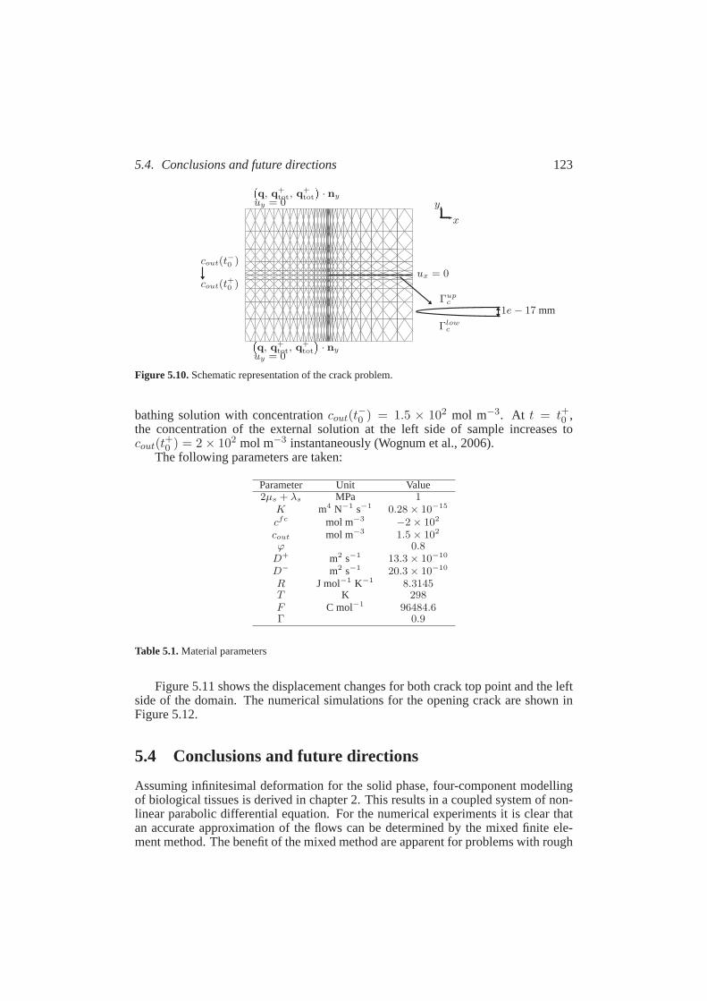
5.4. Conclusions and future directions 123
q, q+
tot, q+tot
· ny
q, q+
tot, q+tot
· ny
ux = 0
uy = 0
uy = 0
x
y
cout(t−
0 )
cout(t+0 )
1e − 17 mmΓup
c
Γlowc
Figure 5.10.Schematic representation of the crack problem.
bathing solution with concentrationcout(t−0 ) = 1.5 × 10² mol m−3. At t = t+0 ,
the concentration of the external solution at the left side of sample increases tocout(t
+0 ) = 2 × 10² mol m−3 instantaneously (Wognum et al., 2006).
The following parameters are taken:
Parameter Unit Value2µs + λs MPa 1
K m4 N−1 s−1 0.28 × 10⁻¹⁵
cfc mol m−3−2 × 10²
cout mol m−3 1.5 × 10²
ϕ 0.8D+ m2 s−1 13.3 × 10⁻¹⁰
D− m2 s−1 20.3 × 10⁻¹⁰
R J mol−1 K−1 8.3145T K 298F C mol−1 96484.6Γ 0.9
Table 5.1.Material parameters
Figure 5.11 shows the displacement changes for both crack top point andthe leftside of the domain. The numerical simulations for the opening crack are shown inFigure 5.12.
5.4 Conclusions and future directions
Assuming infinitesimal deformation for the solid phase, four-component modellingof biological tissues is derived in chapter 2. This results in a coupled system of non-linear parabolic differential equation. For the numerical experiments it is clear thatan accurate approximation of the flows can be determined by the mixed finite ele-ment method. The benefit of the mixed method are apparent for problems with rough
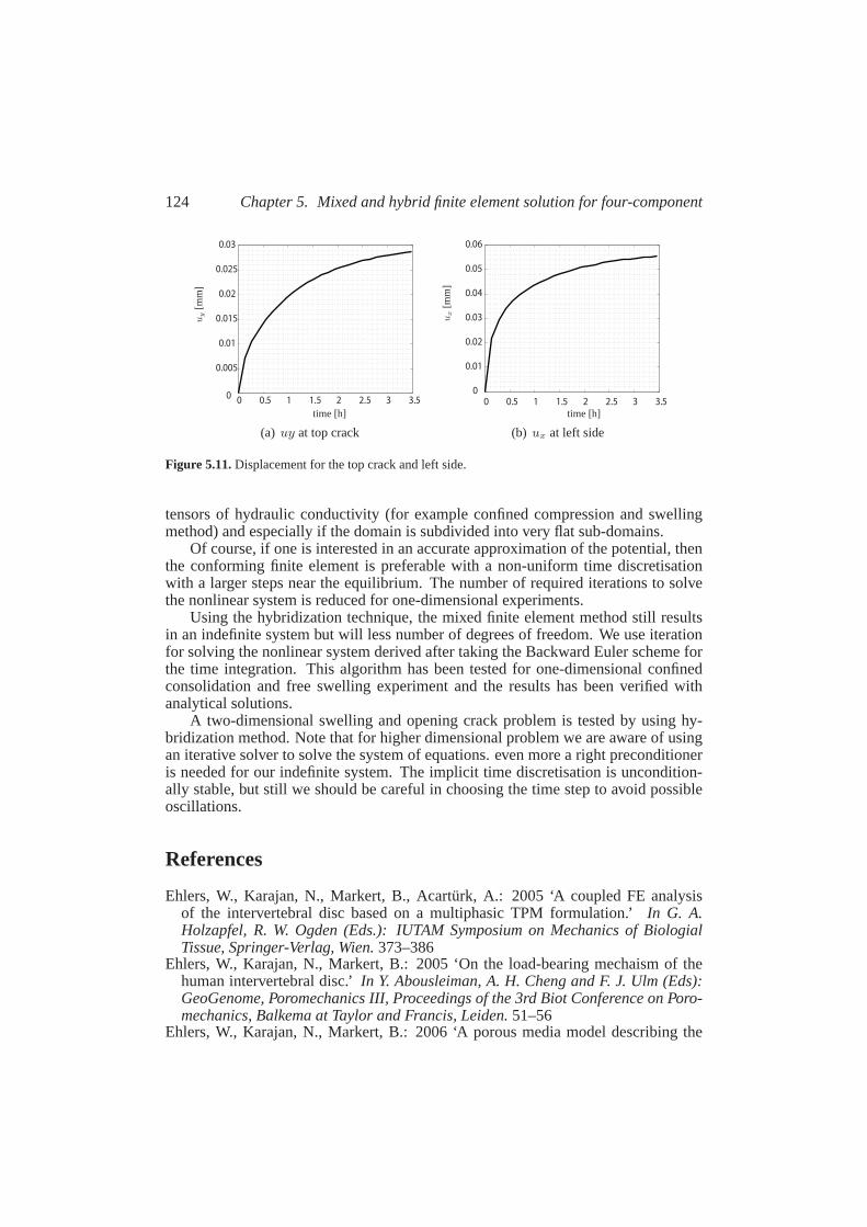
124 Chapter 5. Mixed and hybrid finite element solution for four-component
0 0.5 1 1.5 2 2.5 3 3.50
0.005
0.01
0.015
0.02
0.025
0.03
time [h]
uy
[mm
]
(a) uy at top crack
0 0.5 1 1.5 2 2.5 3 3.5
0
0.01
0.02
0.03
0.04
0.05
0.06
time [h]
ux
[mm
](b) ux at left side
Figure 5.11.Displacement for the top crack and left side.
tensors of hydraulic conductivity (for example confined compression and swellingmethod) and especially if the domain is subdivided into very flat sub-domains.
Of course, if one is interested in an accurate approximation of the potential, thenthe conforming finite element is preferable with a non-uniform time discretisationwith a larger steps near the equilibrium. The number of required iterations to solvethe nonlinear system is reduced for one-dimensional experiments.
Using the hybridization technique, the mixed finite element method still resultsin an indefinite system but will less number of degrees of freedom. We use iterationfor solving the nonlinear system derived after taking the Backward Eulerscheme forthe time integration. This algorithm has been tested for one-dimensional confinedconsolidation and free swelling experiment and the results has been verified withanalytical solutions.
A two-dimensional swelling and opening crack problem is tested by using hy-bridization method. Note that for higher dimensional problem we are aware of usingan iterative solver to solve the system of equations. even more a right preconditioneris needed for our indefinite system. The implicit time discretisation is uncondition-ally stable, but still we should be careful in choosing the time step to avoid possibleoscillations.
References
Ehlers, W., Karajan, N., Markert, B., Acarturk, A.: 2005 ‘A coupled FE analysisof the intervertebral disc based on a multiphasic TPM formulation.’In G. A.Holzapfel, R. W. Ogden (Eds.): IUTAM Symposium on Mechanics of BiologialTissue, Springer-Verlag, Wien.373–386
Ehlers, W., Karajan, N., Markert, B.: 2005 ‘On the load-bearing mechaismof thehuman intervertebral disc.’In Y. Abousleiman, A. H. Cheng and F. J. Ulm (Eds):GeoGenome, Poromechanics III, Proceedings of the 3rd Biot Conference on Poro-mechanics, Balkema at Taylor and Francis, Leiden.51–56
Ehlers, W., Karajan, N., Markert, B.: 2006 ‘A porous media model describing the
References 125
inhomogeneous behaviour of the human intervertebral disc.’Materials Scienceand Materials Technology.37, 546–551
Frijns, A. J. H.: 2001,A four-component mixture theory applied to cartilaginoustissues. PhD-thesis, Eindhoven University of Technology.
Kaasschieter, E. F., Huijben, A. J. M.: 1992, ‘Mixed-hybrid finite elementsandstreamline computation for the potential flow problem.’Numer. Methods PartialDiffer. Equat.8, 221–266.
van Loon, R., Huyghe, J. M., Wijlaars, M. W., Baaijens, F. P. T.: 2003, ‘3D FEimplementation of an incompressible quadriphasic mixture model.’InternationalJournal for Numerical Methods in Engineering57, 1243–1258.
Malakpoor, K., Kaasschieter, E. F., Huyghe, J. M.: 2006, ‘An analytical solution ofincompressible charged porous media.’Zeitschrift fur Angewandte Mathematikund Mechanik.86NO-9, 667–681.
Malakpoor, K., Kaasschieter, E. F., Huyghe, J. M.: 2006, ‘Mathematicalmodellingand numerical solution of swelling of cartilaginous tissues. Part II: Mixed-hybridfinite element solution.’ CASA report, Department of Mathematics and ComputerScience, Technische Universiteit Eindhoven,6-24.
Nedelec, J. C.: 1980, ‘Mixed finite elements inR3.’ Numer. Math.35, 315–341Nedelec, J. C.: 1986, ‘A new familiy of mixed finite elements inR
3.’ Numer. Math.50,57–81
Raviart, P. A., Thomas, J. M.: 1977 ‘A mixed finite element method for 2nd-orderelliptic problems.’Mathematical Aspects of Finite Element Methods, Lecture Notein Mathematics, I. Galligani and E. Magenes, Eds., Springer, BerlinVol 606, 292–315.
Roberts, J. E., Thomas, J. M.: 1991, ‘Mixed and hybrid finite element methods.’Handbook of Numerical Analysis, Volume II: Finite Element Methods,P.G. Ciarletand J.L. Lions, Eds., North Holland, Amsterdam, 523–639.
Rusten, T., Winther, R.: 1992, ‘A Preconditioned Iterative Method for SaddlepointProblems.’SIAM. J. Mat. Anal. Appl.13No 3, 887–904.
Thomas, J. M.: 1977,Sur l’analyse numerique des methods d’elements finis hybridset mixtes.Ph.D. thesis, University Pierre et Marie Curie, Paris.
Wognum, S., Huyghe, J. M., Baaijens, F. P. T.: 2006 ‘Influence of osmoticpressurechanges on the opening of existing cracks in 2 intervertebral disc models’Spine.31, Number 16, 1783–1788
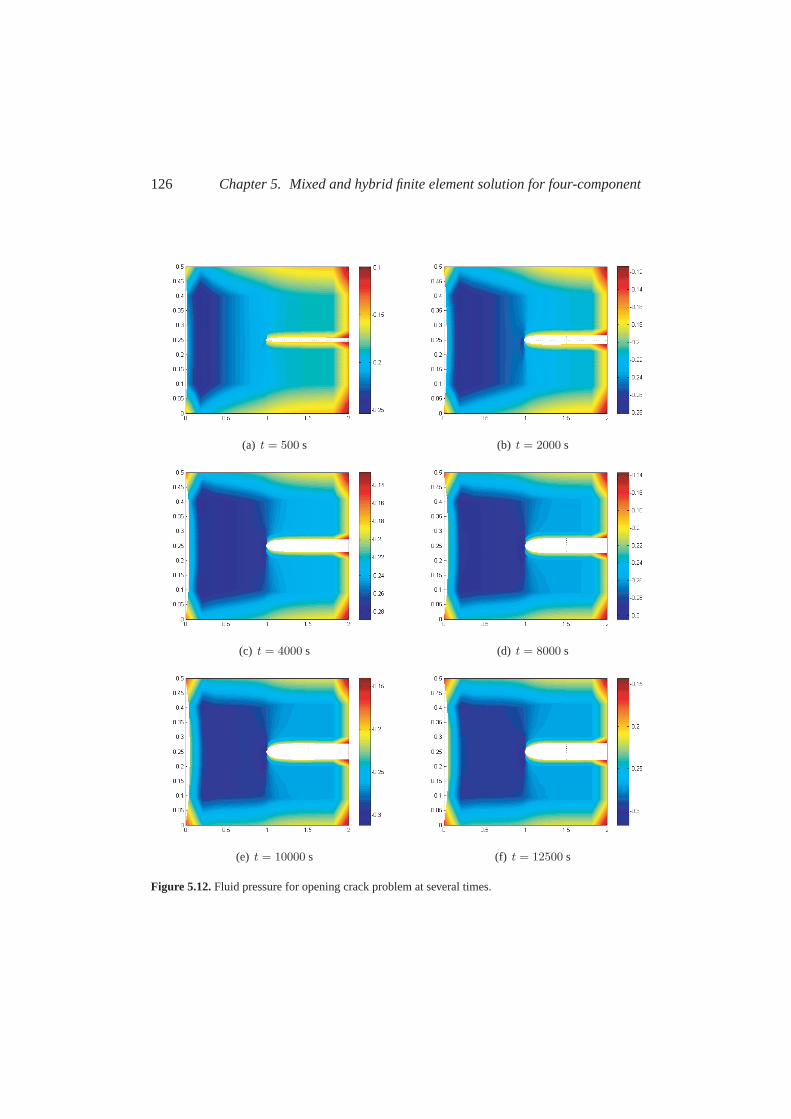
126 Chapter 5. Mixed and hybrid finite element solution for four-component
(a) t = 500 s (b) t = 2000 s
(c) t = 4000 s (d) t = 8000 s
(e) t = 10000 s (f) t = 12500 s
Figure 5.12.Fluid pressure for opening crack problem at several times.
Summary
Mixed Finite Element for Swelling of Cartilaginous Tissues
M any biological porous media exhibit swelling and shrinking behaviour whenincontact with salt concentrations. This phenomenon, observed in cartilageand
hydrogel, is caused by electric charges fixed to the solid, counteracted by correspond-ing charges in fluid. These charges result in a variety of features, including swelling,electro-osmosis, streaming potentials and streaming currents.
Mixture theory is a framework, in which the model integrates mechanical defor-mations, loads, diffusion, convection and chemical reactions of different solutes.
An earlier study from geomechanics presents biphasic models that describe thesolid-fluid interactions. These models cannot describe osmotic effects thathave ma-jor influence on the behaviour of tissues. Therefore to account for osmotic effectsthis is modelled by a four-component mixture theory.
In the four-component mixture theory a deformable and charged porousmediumis saturated with a fluid with dissolved cations and anions. Four components aredefined: solid, liquid, cations and anions. Balance equations for each component aswell as for the mixture are given. Together with the second law of thermodynamics,the constitutive equations are given.
This theory results in a coupled system of nonlinear parabolic differentialequa-tions together with an algebraic constraint for electroneutrality.
In this model, it is desirable to obtain an accurate approximation of the fluid andions flow. Such an accurate approximation can be determined by the mixed finiteelement method.
We consider the numerical solution of the mentioned problem using a mixeddiscretisation by Raviart-Thomas-Nedelec elements on two- and three-dimensionaldomains.
The solid displacement, fluid and ions flow and electro-chemical potentials aretaken as degrees of freedom. This results into a first-order nonlinear algebraic equa-tion with an indefinite coefficient matrix.
The hybridization technique is then used to reduce the list of degrees of freedomand to speed up the numerical computations.
The mixed hybrid finite element method is validated for small deformations usinganalytical solutions for one-dimensional confined consolidation and swelling. Two-dimensional results are shown for a swelling cylindrical hydrogel sample and openingcracks in intervertebral disc.
127

Samenvatting
V eel biologische poreuze media vertonen zwel- en krimpgedrag wanneer deze incontact komen met zoutoplossingen. Dit fenomeen, dat in kraakbeen en hy-
drogel wordt waargenomen, wordt veroorzaakt door elektrische ladingen die aan devaste stof gebonden zijn, die door overeenkomstige ladingen in de vloeistofwordentegengewerkt. Deze ladingen resulteren in een verscheidenheid van verschijnselen,met name zwelling, electro-osmose, stromingspotentialen en elektrische stromingen.
De mengseltheorie is een raamwerk, dat mechanische deformaties, ladingen, dif-fusie, convectie en chemische reacties van verschillende opgeloste stoffen integreert.
Een eerdere geomechanische studie stelt tweefasenmodellen voor, die deinter-actie beschrijven tussen vaste stof en vloeistof. Deze modellen kunnen osmotischeeffecten, die een belangrijke invloed op het gedrag van weefsels hebben, niet beschri-jven. Daarom wordt dit gemodelleerd met de vier-componentenmengseltheorie omosmotische effecten te beschouwen.
In de vier-componentenmengseltheorie is een vervormbaar en geladen poreusmedium verzadigd met een vloeistof met opgeloste kationen en anionen. Vier com-ponenten worden gedefinieerd: vaste stof, vloeistof, kationen en anionen. De bal-answetten voor elke component evenals voor het mengsel worden gegeven. Samenmet de tweede wet van de thermodynamica worden de constitutieve vergelijkingengegeven.
Deze theorie resulteert in een gekoppeld stelsel niet-lineaire parabolische dif-ferentiaalvergelijkingen tezamen met een algebraısche voorwaarde voor elektroneu-traliteit.
In dit model is het wenselijk om een nauwkeurige benadering van de vloeistof-en ionenstroom te verkrijgen. Een dergelijke nauwkeurige benadering kan wordenverkregen met behulp van de gemengde eindige elementenmethode.
We beschouwen de numerieke oplossing van het bovengenoemde probleem ge-bruikmakend van gemengde discretisatie met Raviart-Thomas-Nedelec elementen optwee- en driedimensionale domeinen.
De deformatie, vloeistof- en ionenstroom, en de elektrochemische potentiaalwor-den genomen als graden van vrijheid. Dit resulteert in een eerste orde niet-lineairealgebraısche vergelijking met een indefiniete coefficientenmatrix.
De hybridisatietechniek wordt vervolgens gebruikt om de lijst vrijheidsgraden teverkleinen en de numerieke berekeningen te versnellen.
De gemengdhybride eindige elementenmethode wordt voor kleine vervormingen
129

130 Samenvatting
gevalideerd met hulp van analytische oplossingen voor eendimensionale beperkteconsolidatie en zwelling. Tweedimensionale resultaten worden getoond vooreenmonster van zwellende cilindrische hydrogel en het openbarsten in de tussenwervelsc-hijf.
چکيده
یغضـروفم بافتهای تور برای آميخته هيبريدی روش اجزاء محدود
نمك ـول نمـك متنـاسـب بـا غلظتاورت محلـز مـواد متخلخـل بيولوژيكی در مجبسيـاری ا ـوان ـتخعلت اين پديده آه در نرمه اس. دان مـی دهنــــــای تورمی و انقباضی از خـود نشـــــــــرفتاره
يونهای نظيـر با دجام كلتــــــهای ساآن در اسود، تقابل يونمی شده اهـــــمشدروژل و هي) وفغضـر(، )یمزــالكترو اس( خواص ازجمله تورم، نفوذ الكتريكی از ریـوجود اين يونها يكس .دـمی باشال در سي
. دهدالكتريكی را نتيجه مي ایجريانی و جريانهپتانسيلهای ـال و ار، انتقــــــيير شكل مكانيكی، انتشو تغ حقيقت چهار چوبی است آه درآن بارنظريه آميزه در
.های شيميايی حاللهای متفاوت درآن مطالعه می شودـواآنشيال درآنها ــ آه اندرآنش جامد و سفازی را می توان يافت دو ایــ مطالعات اوليه ژئومكانيك مدلهدر بر رفتار بسزايی مزی يونها آه تاثيرــــدر نظر گرفتن اثرات اس به قادردر حقيقت اين مدلها .است آمدهنظريه چهار مولفه ای آميزه برای در نظر گرفتن اين تاثيرات مورد مطالعه قرار ازاينرو. ا دارند نيستبافته
.می گيردال آه در آن يونهای يـــكل پذير و يونيزه با يك سـنظريه چهار مولفه ای آميزه يك ماده متخلخل ش در
امد، مايع، ــــج: عريف می شوددر اين مدل چهار مولفه ت. حل شده اند اشباع می شود مثبت و منفیادالت توازن برای هر يك از مولفه ها و برای آميزه در نظر گرفته ـــــمع .منفی مثبت و يونهای يونهای
.نيز ارائه می شود معادالت مشخصهترموديناميك تفاده از قانون دومــــبا اس. می شودهموی ــــاز معادالت ديفرانسيل با مشتقات جزئی س هايت اين نظريه يك سيستم غير خطیدر ن
.بهمراه يك قيد جبری برای خنثی سازی الكتريكی بدست می دهدچنين . دــــــميباش آافیا با دقتهدف اصلی در اين مدل محاسبه تقريبی شارسيال و شار يونه
ذآر جواب های عددی مدل. با استفاده از روش اجزاء محدودآميخته بدست آوردتوان ميتـقريبی را - در نظر گرفتن المانهای راويارتبا تفاده از روش گسسته سازی آميخته و ــــــده باال با اســــــــــشـــــ . ندلك برای دامنه های دو و سه بعدی محاسبه می شوند-توماس
ادی ـيميايی به عنوان درجات آزـيلهای الكترو شپتانس ونها وي كلت جامد، شار مايع وتغيير مكان اس در نتيجه يك معادله غير خطی جبری با يك ماتريس ضرايب نامعين . ـوندسيستم در نظر گرفته می شـ
.خواهيم داشتبات عددی ــــــــــــمحاس زايش سرعتافو رای آاستن از تعداد درجات آزادیتكنيك هيبريداسيون ب .ميشود ادهتفاسـدر حالتيكه تغيير ميخته هيبريدی با جوابهای تحليلیآ ت آمده از روش اجزاء محدودــــجوابهای بدس
ائل تحكيم و تورم محدود شده سنجيده ــــــــــشكل فاز جامد بسيار آوچك فرض شده باشد برای مساله باز ـــژل و مستوانه ای شكل از هيدروـنه اسلت دو بعدی برای تورم آزاد يك نمونتايج در حا. ميشوند
.ك بين مهره ها نشان داده می شودـــشدن ترك در ديس
131

Curriculum Vitae
February 13, 1976 Born in Tehran, Iran
September 1994 - September 1998 B. Sc in Pure Mathematics,“Stochastic Groups”,Supervisor: Prof. A. Hassani,Department of Mathematics, Iran Universityof Science and Technology, Tehran, Iran
September 1998 - June 2000 M. Sc in Pure Mathematics,“Homomorphisms and derivations on weight-ed convolution algebras”,Supervisor: Dr. H. R. Farhadi,Department of Mathematics, Sharif Univer-sity of Technology, Tehran, Iran
September 2001 - June 2002 Doctorale Scientiae Mathematicae,“Interpolatory Wavelets”,Supervisor: Prof . K. Urban,Universiteit Utrecht, The Netherlands
September 2002 - February 2007 Ph.D. Researcher in Applied Analysis,“Mixed Finite Element Modelling of Carti-laginous Tissues”,CASA group, Department of Mathematicsand Computer Science, Technische Univer-siteit Eindhoven, The Netherlands
February 2007 - February 2009 Post-doc Researcher,Korteweg de Vries Institute for Mathematics,Universiteit van Amsterdam, The Netherlands
133