23 Find the slope of the sine curve at t = 4 3 from v = cos t. The oscillation x = 0, y = sin t goes (1)up and down (2)between Then find an average slope by dividing sin n/2 -sin 4 3 by -1 and 1 (3) starting from x = 0, y = 0 (4) at velocity the time difference 4 2 -43. v = cos t. Find (1)(2)(3)(4) for the oscillations 31-36.

24 The slope of f = sin t at t = 0 is cos 0 = 1. Compute 31 x=cost, y=O 32 x = 0, y = sin 5t average slopes (sin t)/t for t = 1, .l, .01, .001.

33 x=O, y=2sin(t+O) 34 x=cost, y=cost

The ball at x = cos t, y = sin t circles (1) counterclockwise 35 x=O, y=-2cos i t 36 x=cos2t, y=sin2t (2)with radius 1 (3)starting from x = 1, y = 0 (4)at speed 1. Find (1)(2)(3)(4) for the motions 25-30. 37 If the ball on the unit circle reaches t degrees at time t,

find its position and speed and upward velocity. 25 x=cos3t, y=-sin3t

38 Choose the number k so that x = cos kt, y = sin kt com- 26 x = 3 cos 4t, y = 3 sin 4t pletes a rotation at t = 1. Find the speed and upward velocity. 27 x = 5 sin 2t, y = 5 cos 2t 39 If a pitcher doesn't pause before starting to throw, a balk

is called. The American League decided mathematically that there is always a stop between backward and forward motion, even if the time is too short to see it. (Therefore no balk.) Is

30 x =cos (- t), y = sin (- t) that true?

1.5 A Review of Trigonometry

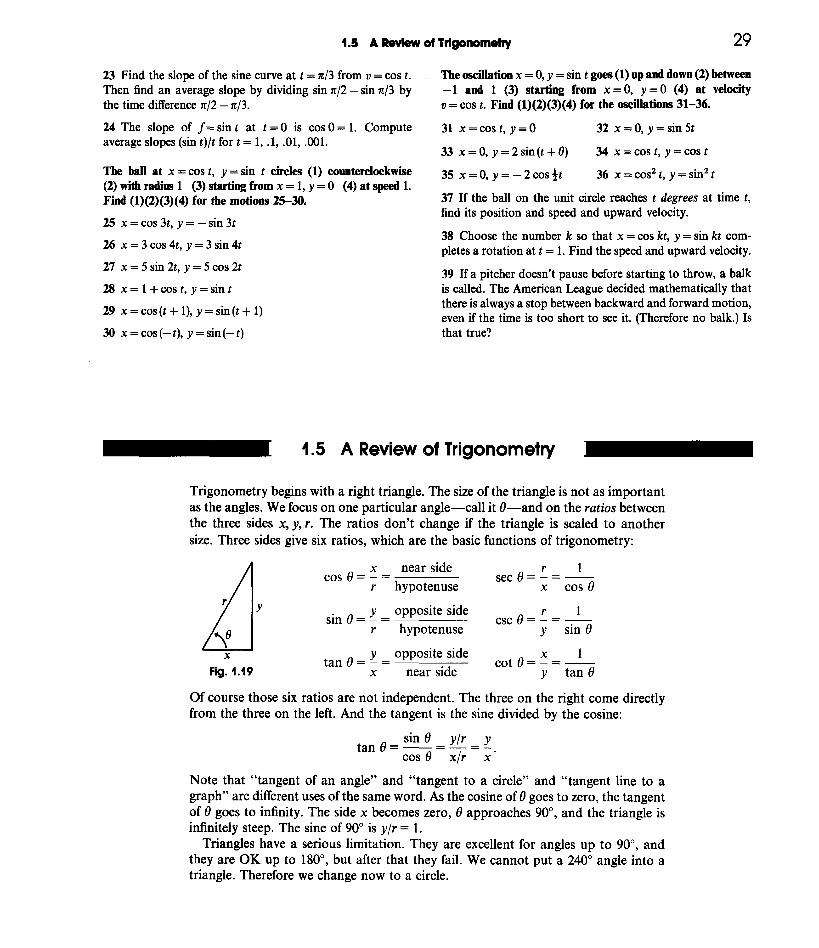
Trigonometry begins with a right triangle. The size of the triangle is not as important as the angles. We focus on one particular angle-call it 8-and on the ratios between the three sides x, y, r. The ratios don't change if the triangle is scaled to another size. Three sides give six ratios, which are the basic functions of trigonometry:

n r 1 cos 8 = -

x =

near side set 8 = - = -r hypo tenuse x cos 8

sin 8 = -y

= opposite side csc 8 = -r = -1

r hypotenuse y sin 8R X

I y y opposite side x 1

tan 8 = - = cot g = - = -Fig. 1.19 x near side y tan 8

Of course those six ratios are not independent. The three on the right come directly from the three on the left. And the tangent is the sine divided by the cosine:

Note that "tangent of an angle" and "tangent to a circle" and "tangent line to a graph" are different uses of the same word. As the cosine of 8 goes to zero, the tangent of 8 goes to infinity. The side x becomes zero, 8 approaches 90", and the triangle is infinitely steep. The sine of 90" is y/r = 1.

Triangles have a serious limitation. They are excellent for angles up to 90°, and they are OK up to 180", but after that they fail. We cannot put a 240" angle into a triangle. Therefore we change now to a circle.

1 Introduction to Calculus

Fig. 1.20 Trigonometry on a circle. Compare 2 sin 8 with sin 28 and tan 8 (periods 2n, n, n).

Angles are measured from the positive x axis (counterclockwise). Thus 90" is straight up, 180" is to the left, and 360" is in the same direction as 0". (Then 450" is the same as 90°.) Each angle yields a point on the circle of radius r. The coordinates x and y of that point can be negative (but never r). As the point goes around the circle, the six ratios cos 8, sin 9, tan 8, .. . trace out six graphs. The cosine waveform is the same as the sine waveform-just shifted by 90".

One more change comes with the move to a circle. Degrees are out. Radians are in. The distance around the whole circle is 2nr. The distance around to other points is Or. We measure the angle by that multiple 8. For a half-circle the distance is m, so the angle is n radians-which is 180". A quarter-circle is 4 2 radians or 90". The distance around to angle 8 is r times 8.

When r = 1 this is the ultimate in simplicity: The distance is 8. A 45" angle is Q of a circle and 27118 radians-and the length of the circular arc is 27~18.Similarly for 1":

360" = 2n radians 1" = 27~1360radians 1 radian = 3601271 degrees.

An angle going clockwise is negative. The angle -n /3 is -60" and takes us 4of the wrong way around the circle. What is the effect on the six functions?

Certainly the radius r is not changed when we go to -8. Also x is not changed (see Figure 1.20a). But y reverses sign, because -8 is below the axis when +8 is above. This change in y affects y/r and y / x but not xlr:

The cosine is even (no change). The sine and tangent are odd (change sign). The same point is 2 of the right way around. Therefore 2 of 2n radians (or 300")

gives the same direction as -n /3 radians or -60". A diflerence of 2n makes no di$erence to x , y, r. Thus sin 8 and cos 8 and the other four functions have period 27~. We can go five times or a hundred times around the circle, adding 10n or 200n to the angle, and the six functions repeat themselves.

EXAMPLE Evaluate the six trigonometric functions at 8 = 2n/3 (or 8 = -4 4 3 ) .

This angle is shown in Figure 1.20a (where r = 1). The ratios are

cos 8 = x/r = -1/2 sin 8 = y/r = &/2 tan 8 = y /x = -& sec e = - 2 csc e = 2/& cot e = -i/d

Those numbers illustrate basic facts about the sizes of four functions:

The tangent and cotangent can fall anywhere, as long as cot 8 = l/tan 8.

1.5 A Review of Ttlgonometry

The numbers reveal more. The tangent -3 is the ratio of sine to cosine. The secant -2 is l/cos 8. Their squares are 3 and 4 (differing by 1). That may not seem remarkable, but it is. There are three relationships in the squares of those six numbers, and they are the key identities of trigonometry:

Everything flows fvom the Pythagoras formula x2 + y2 = r2. Dividing by r2 gives ( ~ / r ) ~+ (y/r)2= 1. That is cos2 8+ sin28= 1. Dividing by x2 gives the second identity, which is 1 + ( y / ~ ) ~ Dividing by y2 gives the third. All three will be needed = ( r / ~ ) ~ . throughout the book-and the first one has to be unforgettable.

DISTANCES AND ADDITION FORMULAS

To compute the distance between points we stay with Pythagoras. The points are in Figure 1.21a. They are known by their x and y coordinates, and d is the distance between them. The third point completes a right triangle.

For the x distance along the bottom we don't need help. It is x, - xl (or Ix2 - x1I since distances can't be negative). The distance up the side is ly2 -y, 1. Pythagoras immediately gives the distance d:

distance between points = d = J(x2 - x , ) ~+ (y2- y1)'. (1)

x=coss y = sin s

Fig. 1.21 Distance between points and equal distances in two circles.

By applying this distance formula in two identical circles, we discover the cosine of s - t. (Subtracting angles is important.) In Figure 1.2 1 b, the distance squared is

d2= (change in x ) ~ + (change in y)*

= (COSs - cos t)* + (sin s - sin t)2. (2) Figure 1 . 2 1 ~ shows the same circle and triangle (but rotated). The same distance squared is

d2= (cos(s - t) - + (sin (s - t))2. (3) Now multiply out the squares in equations (2) and (3). Whenever (co~ine)~ + (sine)2 appears, replace it by 1. The distances are the same, so (2) = (3):

(2) = 1 + 1 - 2 cos s cos t - 2 sin s sin t

1 Introduction to Calculus

After canceling 1 + 1 and then -2, we have the "addition formula" for cos (s - t):

The cosine of s - t equals cos s cos t + sin s sin t. (4)

The cosine of s + t equals cos s cos t - sin s sin t. (5)

The easiest is t = 0. Then cos t = 1 and sin t = 0. The equations reduce to cos s = cos s. To go from (4) to (5) in all cases, replace t by - t. No change in cos t, but a "minus"

appears with the sine. In the special case s = t, we have cos(t + t )= (COS t)(cos t) - (sin t)(sin t). This is a much-used formula for cos 2t:

Double angle: cos 2t = cos2 t - sin2 t = 2 cos2 t - 1 = 1 - 2 sin2 t. (6)

I am constantly using cos2 t + sin2 t = 1, to switch between sines and cosines. We also need addition formulas and double-angle formulas for the sine of s - t

and s + t and 2t. For that we connect sine to cosine, rather than (sine)2 to (co~ine)~. The connection goes back to the ratio y/r in our original triangle. This is the sine of the angle 0 and also the cosine of the complementary angle 7112 - 0:

sin 0 = cos (7112 - 0) and cos 0 = sin (7112 - 0). (7)

The complementary angle is 7112 - 0 because the two angles add to 7112 (a right angle). By making this connection in Problem 19, formulas (4-5-6) move from cosines to sines:

sin (s - t) =sin s cos t - cos s sin t (8)

sin(s + t) = sin s cos t + cos s sin t (9)

sin 2t = sin(t + t) = 2 sin t cos t (10)

I want to stop with these ten formulas, even if more are possible. Trigonometry is full of identities that connect its six functions-basically because all those functions come from a single right triangle. The x, y, r ratios and the equation x2 + y2 = r2 can be rewritten in many ways. But you have now seen the formulas that are needed by ca1culus.t They give derivatives in Chapter 2 and integrals in Chapter 5. And it is typical of our subject to add something of its own-a limit in which an angle approaches zero. The essence of calculus is in that limit.

Review of the ten formulas Figure 1.22 shows d2 = (0 - $)2+ (1 - -12)~.

71 71 71 71 71 71 71 71 71 cos - = cos - cos - + sin -

71 sin - (s - t) sin -= sin - cos - - cos - sin -

6 2 3 2 3 6 2 3 2 3

571 71 71 71 71 571 71 71 71 cos -= cos - cos - - sin - sin - (s + t) sin -= sin - cos - + cos -

71 sin -

6 2 3 2 3 6 2 3 2 3

71 71 71 (2t) sin 2 - = 2 sin - cos -

3 3 3

71 71sin - = cos -71 = 112cos 2 = sin - = -12 (4-0)6 3 6 3

tcalculus turns (6) around to cos2 t =i(1 + cos 2t) and sin2 t =i(1 -cos 2t).

A Review of Ttlgonometry

Fig. 1.22

1.5 EXERCISES Read-through questions

Starting with a a triangle, the six basic functions are the b of the sides. Two ratios (the cosine x/r and the c )

are below 1. Two ratios (the secant r/x and the d ) are above 1. Two ratios (the e and the f ) can take any value. The six functions are defined for all angles 8, by chang- ing from a triangle to a g .

The angle 8 is measured in h . A full circle is 8 = i , when the distance around is 2nr. The distance to angle 8 is

I . All six functions have period k . Going clockwise changes the sign of 8 and I and m . Since cos (- 9) = cos 8, the cosine is n .

Coming from x2+ y2= r2 are the three identities sin2 8 + cos2 8 = 1 and 0 and P . (Divide by r2 and

q and r .) The distance from (2, 5) to (3, 4) is d = s . The distance from (1, 0) to (cos (s -t), sin (s -t)) leads to the addition formula cos (s - t) = t . Changing the sign of t gives cos (s + t) = u . Choosing s = t gives cos 2t = v or w . Therefore i ( l + cos 2t) = x , a formula needed in calculus.

1 In a 60-60-60 triangle show why sin 30" =3. 2 Convert x, 371, -7114 to degrees and 60°, 90°, 270" to

radians. What angles between 0 and 2n correspond to 8 = 480" and 8 = -I0?

3 Draw graphs of tan 8and cot 8 from 0to 2n. What is their (shortest) period?

4 Show that cos 28 and cos2 8 have period n and draw them on the same graph.

5 At 8= 3n/2 compute the six basic functions and check cos2 8 + sin2 8, sec2 0 - tan2 8, csc2 8 -cot2 8.

6 Prepare a table showing the values of the six basic func- tions at 8 = 0, 7114, n/3, ~ / 2 , n.

7 The area of a circle is nr2. What is the area of the sector that has angle 8? It is a fraction of the whole area.

8 Find the distance from (1, 0) to (0, 1)along (a) a straight line (b) a quarter-circle (c) a semicircle centered at (3,i).

9 Find the distance d from (1,O) to (4, &/2) and show on a circle why 6d is less than 2n.

10 In Figure 1.22 compute d2 and (with calculator) 12d. Why is 12d close to and below 2n?

11 Decide whether these equations are true or false:

sin 8 1 +cos 8 (a) ------= ----

1 -cos 8 sin 8

sec 8 + csc 8 = sin 8 + cos 8

(b) tan e +cot e (c) cos 8 -sec 8 = sin 0 tan 8 (d) sin (2n -8) = sin 8

12 Simplify sin (n -O), cos (n-8), sin (n/2 + 8), cos (n/2 + 8).

13 From the formula for cos(2t + t) find cos 3t in terms of cos t.

14 From the formula for sin (2t + t) find sin 3t in terms of sin t.

15 By averaging cos (s - t) and cos (s + t) in (4-5) find a for- mula for cos s cos t. Find a similar formula for sin s sin t.

16 Show that (cos t + i sin t)2 = cos 2t + i sin 2t, if i2 = -1.

17 Draw cos 8 and sec 8 on the same graph. Find all points where cos B = sec 8.

18 Find all angles s and t between 0 and 2n where sin (s + t) = sin s + sin t.

19 Complementary angles have sin 8 = cos (n/2 -8). Write sin@+ t) as cos(n/2 -s - t) and apply formula (4) with n/2 -s instead of s. In this way derive the addition formula (9).

20 If formula (9) is true, how do you prove (8)?

21 Check the addition formulas (4-5) and (8-9) for s = t = n/4.

22 Use (5) and (9) to find a formula for tan (s + t).

34 1 Introduction to Calculus

In 23-28 find every 8 that satisfies the equation. (1) show that the side PQ has length

23 sin 8 = -1 24 sec 8 = -2 d2=a2+b2-2ab cos 8 (law of cosines).

25 sin 8 =cos 8 26 sin 8 =8 32 Extend the same!riangle to a parallelogram with its fourth

27 sec2 8 +csc2 8 = 1 28 tan 8 = 0 corner at R =(a +b cos 0, b sin 8). Find the length squared of

29 Rewrite cos 8 +sin 0 as f i sin(8+4) by choosing the the other diagonal OR.

correct "phase angle" 4. (Make the equation correct at Draw graphs for equations 33-36, and mark three points. 8 =0. Square both sides to check.)

33 y =sin 2x 34 y = 2 sin xx 30 Match a sin x +b cos x with A sin (x +4). From equation 35 y =3 cos 2xx (9) show that a =A cos 4 and b =A sin 4. Square and add to 36 y=sin x+cos x

find A = .Divide to find tan 4 =bla. 37 Which of the six trigonometric functions are infinite at

31 Draw the base of a triangle from the origin 0 = (0'0) to what angles?

P =(a, 0). The third corner is at Q =(b cos 8, b sin 8). What 38 Draw rough graphs or computer graphs of t sin t and are the side lengths OP and OQ? From the distance formula sin 4t sin t from 0 to 2n.

1.6 1-Thousand Points of Light A

The graphs on the back cover of the book show y = sin n. This is very different from y = sin x. The graph of sin x is one continuous curve. By the time it reaches x = 10,000, the curve has gone up and down 10,000/27r times. Those 1591 oscillations would be so crowded that you couldn't see anything. The graph of sin n has picked 10,000 points from the curve-and for some reason those points seem to lie on more than 40 separate sine curves.

The second graph shows the first 1000 points. They don't seem to lie on sine curves. Most people see hexagons. But they are the same thousand points! It is hard to believe that the graphs are the same, but I have learned what to do. Tilt the second graph and look from the side at a narrow angle. Now the first graph appears. You see "diamonds." The narrow angle compresses the x axis-back to the scale of the first graph.

1-

The effect of scale is something we don't think of. We understand it for maps. Computers can zoom in or zoom out-those are changes of scale. What our eyes see

1.6 A Thousand Points of Light

depends on what is "close." We think we see sine curves in the 10,000 point graph, and they raise several questions:

1. Which points are near (0, O)? 2. How many sine curves are there? 3. Where does the middle curve, going upward from (0, 0), come back to zero?

A point near (0,O) really means that sin n is close to zero. That is certainly not true of sin 1 (1 is one radian!). In fact sin 1 is up the axis at .84, at the start of the seventh sine curve. Similarly sin 2 is .91 and sin 3 is .14. (The numbers 3 and .14 make us think of n. The sine of 3 equals the sine of n - 3. Then sin . l4 is near .14.) Similarly sin 4, sin 5, . . . , sin 21 are not especially close to zero.

The first point to come close is sin 22. This is because 2217 is near n. Then 22 is close to 771, whose sine is zero:

sin 22 = sin (7n - 22) z sin (- .01) z - .01.

That is the first point to the right of (0,O) and slightly below. You can see it on graph 1, and more clearly on graph 2. It begins a curve downward.

The next point to come close is sin 44. This is because 44 is just past 14n.

44 z 14n + .02 so sin 44 z sin .02 z .02.

This point (44, sin 44) starts the middle sine curve. Next is (88, sin 88). Now we know something. There are 44 curves. They begin near the heights sin 0,

sin 1, . . . , sin 43. Of these 44 curves, 22 start upward and 22 start downward. I was confused at first, because I could only find 42 curves. The reason is that sin 11 equals - 0.99999 and sin 33 equals .9999. Those are so close to the bottom and top that you can't see their curves. The sine of 11 is near - 1 because sin 22 is near zero. It is almost impossible to follow a single curve past the top-coming back down it is not the curve you think it is.

The points on the middle curve are at n = 0 and 44 and 88 and every number 44N. Where does that curve come back to zero? In other words, when does 44N come very close to a multiple of n? We know that 44 is 14n + .02. More exactly 44 is 14n + .0177. So we multiply .0177 until we reach n:

if N=n/.0177 then 44N=(14n+.0177)N3 14nN+n.

This gives N = 177.5. At that point 44N = 7810. This is half the period of the sine curve. The sine of 7810 is very near zero.

If you follow the middle sine curve, you will see it come back to zero above 7810. The actual points on that curve have n = 44 177 and n = 44 178, with sines just above and below zero. Halfway between is n = 7810. The equation for the middle sine curve is y = sin (nx/78lO). Its period is 15,620-beyond our graph.

Question The fourth point on that middle curve looks the same as the fourth point coming down from sin 3. What is this "double point?" Answer 4 times 44 is 176. On the curve going up, the point is (176, sin 176). On the curve coming down it is (1 79, sin 179). The sines of 176 and 179 difler only by .00003.

The second graph spreads out this double point. Look above 176 and 179, at the center of a hexagon. You can follow the sine curve all the way across graph 2.

Only a little question remains. Why does graph 2 have hexagons? I don't know. The problem is with your eyes. To understand the hexagons, Doug Hardin plotted points on straight lines as well as sine curves. Graph 3 shows y = fractional part of n/2x. Then he made a second copy, turned it over, and placed it on top. That produced graph 4-with hexagons. Graphs 3 and 4 are on the next page.

36 1 Introduction to Calculus

This is called a Moivt pattevn. If you can get a transparent copy of graph 3, and turn it slowly over the original, you will see fantastic hexagons. They come from interference between periodic patterns-in our case 4417 and 2514 and 1913 are near 271. This interference is an enemy of printers, when color screens don't line up. It can cause vertical lines on a TV. Also in making cloth, operators get dizzy from seeing Moire patterns move. There are good applications in engineering and optics-but we have to get back to calculus.

1.7 Computing in Calculus

Software is available for calculus courses-a lot of it. The packages keep getting better. Which program to use (if any) depends on cost and convenience and purpose. How to use it is a much harder question. These pages identify some of the goals, and also particular packages and calculators. Then we make a beginning (this is still Chapter 1) on the connection of computing to calculus.

The discussion will be informal. It makes no sense to copy the manual. Our aim is to support, with examples and information, the effort to use computing to help learning.

For calculus, the gveatest advantage of the computev is to o$er graphics. You see the function, not just the formula. As you watch, f ( x ) reaches a maximum or a minimum or zero. A separate graph shows its derivative. Those statements are not 100% true, as everybody learns right away-as soon as a few functions are typed in. But the power to see this subject is enormous, because it is adjustable. If we don't like the picture we change to a new viewing window.

This is computer-based graphics. It combines numerical computation with gvaphical computation. You get pictures as well as numbers-a powerful combination. The computer offers the experience of actually working with a function. The domain and range are not just abstract ideas. You choose them. May I give a few examples.

EXAMPLE I Certainly x3 equals 3" when x = 3. Do those graphs ever meet again'? At this point we don't know the full meaning of 3", except when x is a nice number. (Neither does the computer.) Checking at x = 2 and 4, the function x3 is smaller both times: 23 is below 3* and 43 = 64 is below 34 = 81. If x3 is always less than 3" we ought to know-these are among the basic functions of mathematics.

1.7 Computing in Calculus

The computer will answer numerically or graphically. At our command, it solves x3 = 3X. At another command, it plots both functions-this shows more. The screen proves a point of logic (or mathematics) that escaped us. If the graphs cross once, they must cross again-because 3" is higher at 2 and 4. A crossing point near 2.5 is seen by zooming in. I am less interested in the exact number than its position-it comes before x = 3 rather than after.

A few conclusions from such a basic example:

1. A supercomputer is not necessary. 2. High-level programming is not necessary. 3. We can do mathematics without completely understanding it.

The third point doesn't sound so good. Write it differently: We can learn mathematics while doing it. The hardest part of teaching calculus is to turn it from a spectator sport into a workout. The computer makes that possible.

EXAMPLE 2 (mental computer) Compare x2 with 2X. The functions meet at x = 2. Where do they meet again? Is it before or after 2?

That is mental computing because the answer happens to be a whole number (4). Now we are on a different track. Does an accident like Z4 = 42 ever happen again? Can the machine tell us about integers? Perhaps it can plot the solutions of xb = bx. I asked Mathernatica for a formula, hoping to discover x as a function of b-but the program just gave back the equation. For once the machine typed HELP icstead of the user.

Well, mathematics is not helpless. I am proud of calculus. There is a new exercise at the end of Section 6.4, to show that we never see whole numbers again.

EXAMPLE 3 Find the number b for which xb = bx has only one solution(at x = b).

When b is 3, the second solution is below 3. When b is 2, the second solution (4) is above 2. If we move b from 2 to 3, there must be a special "double point"-where the graphs barely touch but don't cross. For that particular b-and only for that one value-the curve xb never goes above bx.

This special point b can be found with computer-based graphics. In many ways it is the "center point of calculus." Since the curves touch but don't cross, they are tangent. They have the same slope at the double point. Calculus was created to work with slopes, and we already know the slope of x2. Soon comes xb. Eventually we discover the slope of bx, and identify the most important number in calculus.

The point is that this number can be discovered first by experiment.

EXAMPLE 4 Graph y(x) = ex- xe. Locate its minimum.

The next example was proposed by Don Small. Solve x4 - 1 l x 3 + 5x - 2 = 0.The first tool is algebra-try to factor the polynomial. That succeeds for quadratics, and then gets extremely hard. Even if the computer can do algebra better than we can, factoring is seldom the way to go. In reality we have two good choices:

1. (Mathematics)Use the derivative. Solve by Newton's method. 2. (Graphics)Plot the function and zoom in.

Both will be done by the computer. Both have potential problems! Newton's method is fast, but that means it can fail fast. (It is usually terrific.) Plotting the graph is also fast-but solutions can be outside the viewing window. This particular function is

1 lntroductlon to Calculus

zero only once, in the standard window from -10 to 10. The graph seems to be leaving zero, but mathematics again predicts a second crossing point. So we zoom out before we zoom in.

The use of the zoom is the best part of graphing. Not only do we choose the domain and range, we change them. The viewing window is controlled by four numbers. They can be the limits A <x <B and C d y d D. They can be the coordinates of two opposite corners: (A, C) and (B, D). They can be the center position (a, b) and the scale factors c and d. Clicking on opposite corners of the zoom box is the fastest way, unless the center is unchanged and we only need to give scale factors. (Even faster: Use the default factors.) Section 3.4 discusses the centering transform and zoom transform-a change of picture on the screen and a change of variable within the function.

EXAMPLE 5 Find all real solutions to x4 - 1 lx3 + 5x - 2 =0.

EXAMPLE 6 Zoom out and in on the graphs of y = cos 40x and y = x sin (llx). Describe what you see.

U(AMpLE 7 What does y = (tan x - sin x)/x3 become at x = O? For small x the machine eventually can't separate tan x from sin x. It may give y = 0. Can you get close enough to see the limit of y?

For these examples, and for most computer exercises in this book, a menu-driven system is entirely adequate. There is a list of commands to choose from. The user provides a formula for y(x), and many functions are built in. A calculus supplement can be very useful-MicroCalc or True BASIC or Exploring Calculus or MPP (in the public domain). Specific to graphics are Surface Plotter and Master Grapher and Gyrographics (animated). The best software for linear algebra is MATLAB.

Powerful packages are increasing in convenience and decreasing in cost. They are capable of symbolic computation-which opens up a third avenue of computing in calculus.

SYMBOLIC COMPUTATION

In symbolic computation, answers can be formulas as well as numbers and graphs. The derivative of y = x2 is seen as "2x." The derivative of sin t is "cos t." The slope of bx is known to the program. The computer does more than substitute numbers into formulas-it operates directly on the formulas. We need to think where this fits with learning calculus.

In a way, symbolic computing is close to what we ourselves do. Maybe too close- there is some danger that symbolic manipulation is all we do. With a higher-level language and enough power, a computer can print the derivative of sin(x2). So why learn the chain rule? Because mathematics goes deeper than "algebra with formulas." We deal with ideas.

I want to say clearly: Mathematics is not formulas, or computations, or even proofs, but ideas. The symbols and pictures are the language. The book and the professor and the computer can join in teaching it. The computer should be non-threatening (like this book and your professor)-you can work at your own pace. Your part is to learn by doing.

EXAMPLE 8 A computer algebra system quickly finds 100 factorial. This is loo! = (100)(99)(98)... (1). The number has 158 digits (not written out here). The last 24

1.7 Computing In Calculus

digits are zeros. For lo! = 3628800 there are seven digits and two zeros. Between 10 and 100, and beyond, are simple questions that need ideas:

1. How many digits (approximately) are in the number N!? 2. How many zeros (exactly) are at the end of N!?

For Question 1,the computer shows more than N digits when N = 100. It will never show more than N2 digits, because none of the N terms can have more than N digits. A much tighter bound would be 2N, but is it true? Does N! always have fewer than 2N digits?

For Question 2, the zeros in lo! can be explained. One comes from 10, the other from 5 times 2. (10 is also 5 times 2.) Can you explain the 24 zeros in loo!? An idea from the card game blackjack applies here too: Count the$ves.

Hard question: How many zeros at the end of 200!?

The outstanding package for full-scale symbolic computation is Mathematica. It was used to draw graphs for this book, including y = sin n on the back cover. The complete command was List Plot [Table [Sin [n], (n, 10000)]]. This system has rewards and also drawbacks, including the price. Its original purpose, like MathCAD and MACSYMA and REDUCE, was not to teach calculus-but it can. The computer algebra system MAPLE is good.

As I write in 1990, DERIVE is becoming well established for the PC. For the Macintosh, Calculus TIL is a "sleeper" that deserves to be widely known. It builds on MAPLE and is much more accessible for calculus. An important alternative is Theorist. These are menu-driven (therefore easier at the start) and not expensive.

I strongly recommend that students share terminals and work together. Two at a terminal and 3-5 in a working group seems to be optimal. Mathematics can be learned by talking and writing-it is a human activity. Our goal is not to test but to teach and learn.

Writing in Calculus May I emphasize the importance of writing? We totally miss it, when the answer is just a number. A one-page report is harder on instructors as well as students-but much more valuable. A word processor keeps it neat. You can't write sentences without being forced to organize ideas-and part of yourself goes into it.

I will propose a writing exercise with options. If you have computer-based graph- ing, follow through on Examples 1-4 above and report. Without a computer, pick a paragraph from this book that should be clearer and make it clearer. Rewrite it with examples. Identify the key idea at the start, explain it, and come back to express it differently at the end. Ideas are like surfaces-they can be seen many ways.

Every reader will understand that in software there is no last word. New packages keep coming (Analyzer and EPIC among them). The biggest challenges at this moment are three-dimensional graphics and calculus workbooks. In 30, the problem is the position of the eye-since the screen is only 20. In workbooks, the problem is to get past symbol manipulation and reach ideas. Every teacher, including this one, knows how hard that is and hopes to help.

GRAPHING CALCULATORS

The most valuable feature for calculus-computer-based graphing-is available on hand calculators. With trace and zoom their graphs are quite readable. By creating the graphs you subconsciously learn about functions. These are genuinely personal computers, and the following pages aim to support and encourage their use.

1 Introduction to Calculus

Programs for a hand-held machine tend to be simple and short. We don't count the zeros in 100 factorial (probably we could). A calculator finds crossing points and maximum points to good accuracy. Most of all it allows you to explore calculus by yourself. You set the viewing window and define the function. Then you see it.

There is a choice of calculators-which one to buy? For this book there was also a choice-which one to describe? To provide you with listings for useful programs, we had to choose. Fortunately the logic is so clear that you can translate the instruc- tions into any language-for a computer as well as a calculator. The programs given here are the "greatest common denominator" of computing in calculus.

The range of choices starts with the Casio fx 7000G-the first and simplest, with very limited memory but a good screen. The Casio 7500,8000, and 8500 have increas- ing memory and extra features. The Sharp EL-5200 (or 9000 in Canada and Europe) is comparable to the Casio 8000. These machines have algebraic entry-the normal order as in y = x + 3. They are inexpensive and good. More expensive and much more powerful are the Hewlett-Packard calculators-the HP-28s and HP-48SX. They have large memories and extensive menus (and symbolic algebra). They use reverse Polish notation-numbers first in the stack, then commands. They require extra time and effort, and other books do justice to their amazing capabilities. It is estimated that those calculators could get 95 on a typical calculus exam.

While this book was being written, Texas Instruments produced a new graphing calculator: the TI-81. It is closer to the Casio and Sharp (emphasis on graphing, easy to learn, no symbolic algebra, moderate price). With earlier machines as a starting point, many improvements were added. There is some risk in a choice that is available only At before this textbook is published, and we hope that the experts we asked are right. Anyway, our programs are Jbr the TI-81. It is impressive.

These few pages are no substitute for the manual that comes with a calculator. A valuable supplement is a guide directed especially at calculus-my absolute favorites are Calculus Activities for Graphic Calculators by Dennis Pence (PWS-Kent, 1990 for the Casio and Sharp and HP-28S, 1991 for the TI-81). A series of Calculator Enhance- ments, using HP's, is being published by Harcourt Brace Jovanovich. What follows is an introduction to one part of a calculus laboratory. Later in the book, we supply TI-81 programs close to the mathematics and the exercises that they are prepared for.

A few words to start: To select from a menu, press the item number and E N T E R . Edit a command line using D E L(ete) and I N S(ert). Every line ends with E N T E R . For calculus select radians on the M 0 D E screen. For powers use * . For special powers choose x2, x- l , &.Multiplication has priority, so (-)3 + 2 x 2 produces 1. Use keys for S I N , I F , I S, .. . When you press letters, I multiplies S .

If a program says 3 + C , type 3 S T 0 C E N T E R . Storage locations are A to Z or Greek 8.

Functions A graphing calculator helps you (forces you?) to understand the concept of a function. It also helps you to understand specific functions-especially when changing the viewing window.

To evaluate y = x2 - 2x just once, use the home screen. To define y(x) for repeated use, move to the function edit screen: Press M 0 D E, choose F u n c t io n, and press Y =. Then type in the formula. Important tip: for X on the TI-81, the key X I T is faster than two steps A L p h a X. The Y = edit screen is the same place where the formula is needed for graphing.

1.7 Computing in Calculus

Example Y I = X ~ - ~ XENTERontheY=screen. 4 ST0 X ENTERonthehome screen. Y 1 E N T E R on the Y-VARS screen. The screen shows 8, which is Y(4). The formula remains when the calculator is off.

Graphing You specify the X range and Y range. (We should say X domain but we don't.) The screen is a grid of 96 x 64 little rectangles called "pixels." The first column of pixels represents X m i n and the last column is X m a x . Press R A N G E to reset. With X r e s = 1 the function is evaluated 96 times as it is graphed. X s c L and Y s c L give the spaces between ticks on the axes.

The Z 0 0 M menu is a fast way to set ranges. Z 0 0 M S t a n d a r d gives the default -1O<x<10, -10<y<10. Z O O M T r i g gives - 2 n < x < h , - 3 < y < 3 .

The keystroke G R A P H shows the graphing screen with the current functions.

Example Set the ranges (-)2 < X < 3 and (-) 150 < Y 6 50. Press Y = and store Y1 = X (in ~ A T H ) ~ - 2 8 X ~ + l 5 ~ + 3 6 E N T E R . Press GRAPH. You won't see much of the graph! Press R A N G E and reset (-)I 0 < X < 30, (-)4000 < Y < 2300. Press G R A P H. See a cubic polynomial.

"Smart Graph" recalls the graph instantly without redrawing it, if no settings have changed. The D R A W menu is for points, lines, and shaded regions. This is perfect for our piecewise linear functions-just connect the breakpoints with lines. In Section 3.6 the lines show an iteration by its "cobweb."

Programming This book contains programs that you can type in once and save. We chose Autoscaling, Newton's Method, Secant Method, Cobweb Iteration, and Numerical Integration. You will create others-to do calculations or to add features that are not available as single keystrokes. The calculator is like a computer, with a fairly small set of instructions. One digerence: Memory is too precious to store com- ments with the code. You have to see the logic by rereading the program.

To enter the world of programming, press P R G M. Each P R G M submenu lists all programs by name-a digit, a letter, or 6 (37 names). The program title has up to eight characters. Select the E D I T submenu and press G for the edit screen. Type the title G R A P H S and press E N T E R . Practice on this one:

: " x ~ + x " ST0 (Y-VARS) Y1 ENTER :"X-1" ST0 (Y-VARS) Y2 ENTER : ( P R G M ) ( I / O l D i s p G r a p h

The menus to call are in parentheses. Leave the edit screen with Q U I T (not C L E A R -that erases the line with the cursor). Set the default window by Z 0 0 M S t a n d a r d .

To execute, press P R G M ( E X E C G E N T E R . The program draws the graphs. It leaves Y 1 and Y 2 on the Y = screen. To erase the program from the home screen, press (PRGM)(ERASE)G. Practice again by creating P r gw 2 :F U N C . Type:TXST0 Y and : (PRGM) ( I / O ) D i s p Y. Movetothehomescreen,store X by 4 ST0 X ENTER, and execute by (PRGM) (EXEC12 ENTER. Also try X = - 1. When it fails to imagine i, select 1 :G o t o E r r o r .

Piecewise functions and Input (to a running program). The definition of a piecewise function includes the domain of each piece. Logical tests like " I F X 2 7 " determine which domain the input value X falls into. An I F statement only affects the following line-which is executed when T E S T = 1 (meaning true) and skipped when T E S T =0 (meaning false). I F commands are in the P R G M ( C T L submenu; T E S T calls the menu of inequalities.

1 Introduction to Calculus

An input value X = 4 need not be stored in advance. Program P stops while running to request input. Execute with P E N T E R after selecting the P R G M ( E X E C > menu. Answer ? with 4 and E N T E R. After completion, rerun by pressing E N T E R again. The function is y = 14 - x if x < 7, y = x if x > 7.

P r g m P : P I E C E S :Di s p " x = " P G R M (I1 0 ) Ask for input : I n p u t X PGRM ( 1 1 0 ) Screen ? E N T E R X : 1 4 - X - + Y First formula for all X : I f 7 < X PRGM ( C T L ) T E S T : X + Y Overwrite if T E S T = 1 :D i s p Y Display Y(X)

Overwriting is faster than checking both ends A <X <B for each piece. Even faster: a whole formula (14 -X)(X < 7) + (X)(7 <X) can go on a single line using 1 and 0 from the tests. Compute-store-display Y(X) as above, or define Y 1 on the edit screen.

Exercise Define a third piece Y = 8 + X if X < 3. Rewrite P using Y 1 = . A product of tests ( 3 < X > ( X < 7 1 evaluates to 1 if all true and to 0 if any false.

TRACE and ZOOM The best feature is graphing. But a whole graph can be like a whole book-too much at once. You want to focus on one part. A computer or calculator will trace along the graph, stop at a point, and zoom in.

There is also Z 0 0 M 0 U T, to widen the ranges and see more. Our eyes work the same way-they put together information on different scales. Looking around the room uses an amazingly large part of the human brain. With a big enough computer we can try to imitate the eyes-this is a key problem in artificial intelligence. With a small computer and a zoom feature, we can use our eyes to understand functions.

Press T R A C E to locate a point on the graph. A blinking cursor appears. Move left or right-the cursor stays on the graph. Its coordinates appear at the bottom of the screen. When x changes by a pixel, the calculator evaluates y(x). To solve y(x) = 0, read off x at the point when y is nearest to zero. To minimize or maximize y(x), read off the smallest and largest y. In all these problems, zoom in for more accuracy.

To blow up a figure we can choose new ranges. The fast way is to use a Z 0 0 M command. Forapresetrange,use Z O O M S t a n d a r d or Z O O M T r ig.Toshrink or stretch by X F a c t or Y F a c t (default values 4), use Z 0 0 M In or Z 0 0 M 0 u t . Choose the center point and press E N T E R. The new graph appears. Change those scaling factors with Z 0 0 M S e t F a c t o r s . Best of all, create your own viewing window. Press Z 0 0 M Bo x .

To draw the box, move the cursor to one corner. Press E N T E R and this point is a small square. The same keys move a second (blinking) square to the opposite corner-the box grows as you move. Press E N T E R, and the box is the new viewing window. The graphs show the same function with a change of scale. Section 3.4 will discuss the mathematics-here we concentrate on the graphics.

EXAMPLE9 Place : Y l = X s i n ( 1 / X I intheY=editscreen.PressZOOM T r i g for a first graph. Set X F a c t = 1 and Y F a c t = 2.5. Press Z 0 0 M In with center at (O,O).Toseealargerpicture,use X F a c t = 10and Y F a c t = 1.Then Zoom Out again. As X gets large, the function X sin ( l /X) approaches .

Now return to Z 0 0 M T r i g . Z o o m In with the factors set to 4 (default). Zoom again by pressing E N T E R. With the center and the factors fixed, this is faster than drawing a zoom box.

1.7 Computing in Calculus

EXAMPLE 10 Repeat for the more erratic function Y = sin (l/X). After Z0 0 M Tr ig , create a box to see this function near X = .01. The Y range is now

Scaling is crucial. For a new function it can be tedious. A formula for y(x) does not easily reveal the range of y's, when A <x <B is given. The following program is often more convenient than zooms. It samples the function L= 19 times across the x-range (every 5 pixels). The inputs Xmin, Xmax, Y, are previously stored on other screens. After sampling, the program sets the y-range from C = Ymin to D = Ymax and draws the graph.

Notice the loop with counter K. The loop ends with the command I S > ( K,L , which increases K by 1 and skips a line if the new K exceeds L. Otherwise the command G o t o 1 restarts the loop. The screen shows the short form on the left.

Example: Y l =x3+10x2-7x+42 with range Xrnin=-12 and Xrnax=lO. Set tick spacing X s c l = 4 and Yscl=250. Execute with PRGM (EXEC) A E NTE R. For this program we also list menu locations and comments.

PrgmA :AUTOSCL Menu (Submenu) Comment : A l l - O f f Y -V A R S ( 0 F F Turn off functions :Xm in+A V A R S (RNG) Store X m i n using ST0 : 1 9 + L Store number of evaluations (19) : (Xmax-A) / L + H Spacing between evaluations : A + X Start at x = A :Y1 + C Y -V A R S ( Y ) Evaluate the function : C + D Start C and D with this value :I+K Initialize counter K = 1 : L b l I PR G M ( C TL ) Mark loop start :AtKH + X Calculate next x :Y1 + Y Evaluate function at x : I F Y < C PGRM (CTL) New minimum? : Y + C Update C : I F D c Y PRGM (CTL) New maximum? : Y + D Update D : I S > (K,L) PRGM (CTL) Add 1 to K, skip G o t o if > L : G o t o 1 PRGM (CTL) Loop return to L b l 1 :YI-On Y - V A R S ( O N ) Turnon Y1 :C+Ymin ST0 V A R S ( R N G ) Set Y m i n = C :D+Ymax ST0 V A R S (RNG) Set Ymax=D : D i s p G r a p h PR G M ( I/ 0 1 Generate graph

MIT OpenCourseWare http://ocw.mit.edu

Resource: Calculus Online Textbook Gilbert Strang

The following may not correspond to a particular course on MIT OpenCourseWare, but has been provided by the author as an individual learning resource.

For information about citing these materials or our Terms of Use, visit: http://ocw.mit.edu/terms.