mist international journal of science and technology
TRANSCRIPT


MIJST
MIST International Journal of Science and Technology


iii
EDITORIAL BOARD
CHIEF PATRON
Major General Md Wahid-Uz-Zaman, ndc, aowc, psc, te Commandant Military Institute of Science and Technology (MIST) Dhaka, Bangladesh
EDITOR-IN-CHIEF
Dr. Firoz Alam Professor School of Engineering, RMIT University Melbourne, Australia
EXECUTIVE EDITOR
Dr. A.K.M. Nurul Amin Professor, Industrial and Production Engineering, Military Institute of Science and Technology Dhaka, Bangladesh ASSOCIATE EDITORS
Lt Col Md Altab Hossain, PhD, EME Assoc. Professor, Nuclear Science and Engineering, Military Institute of Science and Technology Dhaka, Bangladesh
Lt Col Muhammad Nazrul Islam, PhD, Sigs Assoc. Professor, Computer Science and Engineering, Military Institute of Science and Technology Dhaka, Bangladesh COPY EDITOR
Dr. Md Enamul Hoque Professor, Biomedical Engineering, Military Institute of Science and Technology Dhaka, Bangladesh EDITORIAL ADVISOR
Col Molla Md. Zubaer, te Military Institute of Science and Technology Dhaka, Bangladesh
SECTION EDITORS
Dr G. M Jahid Hasan Professor (CE), MIST, Dhaka, Bangladesh
Lt Col Khondaker Sakil Ahmed, PhD Assoc. Professor (CE), MIST, Dhaka, Bangladesh
Dr. Md. Mahbubur Rahman Professor (CSE), MIST, Dhaka, Bangladesh
Brig Gen A K M Nazrul Islam, PhD Professor (EECE), MIST, Dhaka, Bangladesh
Mr. Tariq Mahbub Assist. Professor (ME), MIST, Dhaka, Bangladesh
Dr. M A Taher Ali Professor (AE), MIST, Dhaka, Bangladesh
Dr M A Rashid Sarker Professor (NSE), MIST, Dhaka, Bangladesh
Maj Osman Md Amin, PhD, Engrs Assoc. Professor (NAME), MIST, Dhaka, Bangladesh
Maj Kazi Shamima Akter, PhD, Engrs Assoc. Professor (EWCE), MIST, Dhaka, Bangladesh
Md. Sazzad Hossain Assoc. Professor (Arch), MIST, Dhaka, Bangladesh
Dr. Md Enamul Hoque Professor (BME), MIST, Dhaka, Bangladesh
Dr. Muammer Din Arif Assist. Professor (IPE), MIST, Dhaka, Bangladesh
Dr. AKM Badrul Alam Assoc. Professor (PME), MIST, Dhaka, Bangladesh
Lt Col Brajalal Sinha, PhD, AEC Assoc. Professor (Sc & Hum), MIST, Dhaka, Bangladesh
Lt Col Palash Kumar Sarker, PhD, Sigs Assoc. Professor (Sc & Hum), MIST, Dhaka, Bangladesh

iv
PROOF/LANGUAGE SUPPORT GROUP
Maj Md. Manwarul Haq, PhD, AEC Associate Professor Science & Humanities, Military Institute of Science and Technology Dhaka, Bangladesh
Selin Yasmin Associate Professor Science & Humanities, Military Institute of Science and Technology Dhaka, Bangladesh
Md Moslem Uddin Librarian, Military Institute of Science and Technology Dhaka, Bangladesh
RESEARCH COORDINATOR
Lt Col Muhammad Sanaullah, psc, Engrs GSO-1, R&D Wing, Military Institute of Science and Technology Dhaka, Bangladesh
WEB CONSULTANT
Dr. M. Akhtaruzzaman Assistant Professor, CSE, Military Institute of Science and Technology Dhaka, Bangladesh
EDITORIAL BOARD MEMBERS (EXTERNAL)
Dr. Md Hadiuzzaman Professor, Bangladesh University of Engineering & Technology (BUET), Bangladesh
Dr. M. Kaykobad Professor, Bangladesh University of Engineering & Technology (BUET), Bangladesh
Dr. A.B.M. Harun-ur Rashid Professor, Bangladesh University of Engineering & Technology (BUET), Bangladesh
Dr. Abdul Hasib Chowdhury Professor, Bangladesh University of Engineering & Technology (BUET), Bangladesh
Dr. Mohammad Ali Professor, Bangladesh University of Engineering & Technology (BUET), Bangladesh
Dr. Nikhil Ranjan Dhar Professor, Bangladesh University of Engineering & Technology (BUET), Bangladesh
Dr. Shahjada Tarafder Professor, Bangladesh University of Engineering & Technology (BUET), Bangladesh
Dr. Tanvir Ahmed Professor, Bangladesh University of Engineering & Technology (BUET), Bangladesh
Dr. Khandaker Shabbir Ahmed Professor, Bangladesh University of Engineering & Technology (BUET), Bangladesh
Dr. Nahrizul Adib Bin Kadri Assoc. Professor, University of Malaya, Malaysia
Dr. Sunil S. Chirayath Assoc. Professor, Texas A&M University, USA
Dr. A.K.M. Masud Professor, Bangladesh University of Engineering & Technology (BUET), Bangladesh
Dr. ASM Woobaidullah Professor, Dhaka University, Bangladesh
Dr. Abdul Basith Professor, Bangladesh University of Engineering & Technology (BUET), Bangladesh
Dr. Md Abdul Jabbar Professor, Dhaka University, Bangladesh

v
INTERNATIONAL ADVISORY BOARD MEMBERS
Dr. Mahmud Ashraf Assoc. Professor, Deakin University, Australia
Dr. Mohammed A Quddus Professor, Loughborough University, UK
Dr. A. K. M. Najmul Islam Adjunct Professor, University of Turku, Finland
Dr. Chanchal Roy Professor, University of Saskatchewan, Canada
Dr. Muhammad H. Rashid Professor, University of West Florida, USA
Dr. Md. Azizur Rahman Adjunct Professor, Memorial University of Newfoundland, Canada
Dr. Ing. Bhuiyan Shameem Mahmood Ebna Hai Scientific Researcher, Helmut-Schmidt-Universitat, Germany
Dr. Naoya Umeda Professor, Osaka University, Japan
Dr. Easir Arafat Papon University of Alabania, Alabania
Dr. Kawamura Yasumi Professor, Yokohama National University, Japan
Dr. Navid Saleh Assoc. Professor, The University of Texas at Austin, USA
Dr. Soumyen Bandyopadhyay Professor, Liverpool University, UK
Dr. Hafizur Rahman Research Fellow, Curtin University, Australia
Dr. Rezaul Karim Begg Professor, University of Victoria, Australia
Dr. Subramani Kanagaraj Professor, IIT, Guwahati, India
Dr. Mohamed H. M. Hassan Professor, Alexandria University, Egypt
Dr. Ahmad Faris Ismail Professor, International Islamic University Malaysia (IIUM), Malaysia
Dr. Azizur Rahman Assistant Professor, Texas A&M University, Qatar
Dr. Stephen Butt Professor, Memorial University of Newfoundland Canada
Dr. Basir Ahmmad Professor, Yamagata University, Japan.
D-T. Ngo Technical University of Denmark, Denmark
Dr. Kobayahsi Kensei Professor, Yokohama National University, Japan
Dr. Md Ataur Rahman Professor, International Islamic University Malaysia (IIUM), Malaysia
Dr. Cheol-Gi Kim Professor, Daegu Gyeongbuk Institute of Science & Technology, Korea
Dr. Bashir Khoda Assistant Professor, The University of MAINE, USA
DISCLAIMER
The analysis, opinions, and conclusions expressed or implied in this Journal are those of the authors and do not necessarily represent the views of the MIST, Bangladesh Armed Forces, or any other agencies of Bangladesh Government. Statements of fact or opinion appearing in MIJST Journal are solely those of the authors and do not imply endorsement by the editors or publisher. ISSN: 2224-2007 E-ISSN: 2707-7365 QUERIES ON SUBMISSION
For any query on submission the author(s) should contact: MIST, Mirpur Cantonment, Dhaka-1216, Bangladesh; Tel: 88 02 8034194, FAX: 88 02 9011311, email: [email protected]. For detailed information on submission of articles, the author(s) should refer to the Call for Papers and About MIJST at the back cover of the MIJST Journal. Authors must browse MIJST website through the journal link (https://mijst.mist.ac.bd/mijst) for electronic submission of their manuscripts. PUBLISHER
Military Institute of Science and Technology (MIST), Dhaka, Bangladesh All rights reserved. No part of this publication may be reproduced, stored in retrieval system, or transmitted in any form, or by any means, electrical, photocopying, recording, or otherwise, without the prior permission of the publisher. DESIGN AND PRINTING
Research and Development Wing Military Institute of Science and Technology (MIST) Dhaka, Bangladesh


vii
MESSAGE
ARMY HEADQUARTERS DHAKA CANTONMENT
Military Institute of Science and Technology (MIST) has taken a praiseworthy effort towards
transforming its previous Journal – ‘MIST Journal of Science and Technology’ into an international journal
founded on an Open Journal platform. The objective of the new Journal is to add value to the field of
science and engineering. I appreciate timely initiative in upgrading MIST’s Flagship Journal to ‘Online
Peer Reviewed Open Access.’ The contents of ‘MIST International Journal of Science and Technology
(MIJST)’ aptly reflect MIST’s reputation and quality.
I am pleased that the launching of the December 2020 Issue of MIJST has been synchronized with the
Victory Day of Bangladesh. Henceforth, it shall be published as the ‘Victory Day Issue’ to pay tribute to all
the Martyrs and the Freedom Fighters of the Liberation War of Bangladesh. On this occasion, I also
express my solemn respect and homage to the Father of the Nation, Bangabandhu Sheikh Mujibur
Rahman on his centennial birth anniversary.
I wish MIJST’s success in its noble mission of achieving the reputation of an international journal through
meaningful research and dissemination of outputs in the field of cutting-edge Science and Technology!
________________
AZIZ AHMED General Chief of Army Staff Bangladesh Army

viii

ix
FOREWORD
Bismillahir Rahmanir Rahim
The Military Institute of Science and Technology (MIST) being a dynamic academic institution with a
vision of achieving excellence in teaching and cutting-edge research in the areas of science, engineering,
and technology plays an active role in the dissemination of quality research outputs of the institution and
those of the national and international community through its flagship journal - ‘MIST International
Journal of Science and Technology (MIJST)’.
The Journal team worked hard to be able to publish the December issue of MIJST on the Victory Day of
Bangladesh which so special to us. We pay our solemn respect to the 30 million Bengalis who laid their
precious lives to free our motherland from the occupation of the Pakistani Army. We also pay our
homage and deep respect to our Father of the Nation, the Architect of Bangladesh - ‘Bangabandhu Sheikh
Mujibur Rahman’ on His 100th Birth Anniversary.
I would like to take this opportunity to thank the MIJST team for their hard work and express my deep
appreciation to the Authors of the issue, and the associated personnel for their tireless efforts and
contributions to the December Issue 2020 of MIJST. Sincere appreciation to all the reviewers for
providing invaluable peer review to the articles published in this issue to ensure high quality. Very
special thanks to the National and the International Advisory Boards for their invaluable suggestions and
guidance in maintaining the quality of the Journal.
I wish continued success of MIJST.
___________________________________________________________________
Major General Md Wahid-Uz-Zaman, ndc, aowc, psc, te Commandant, MIST, Bangladesh Chief Patron, MIJST, Bangladesh


xi
EDITORIAL
Despite the difficulties posed by global COVID-19 pandemic; the second (December 2020) issue of MIST
International Journal of Science and Technology (MIJST) has been published well within the schedule. I
am pleased to note that this was possible thanks to the hard work and consolidated efforts undertaken by
the authors, the reviewers, and the editorial & production teams whose commitment, synergy, love, and
vision for the Journal are unwavering. The journal remains fully committed to publishing contemporary
and innovative theoretical and applied research outputs in the fields of science, engineering, and
technology, which makes MIJST a true interdisciplinary journal.
The MIJST is a bi-annual and Open Access Journal. The Open Access policy enables the journal to be
accessed by all readers and makes it more visible and globally accessible facilitating diffusion of new
knowledge and innovations. Furthermore, authors and readers do not need to incur any cost for the
publication and getting access to the journal. Inclusion of the Journal in several Indexing Databases, such
as, ‘Google Scholar’, ‘DOI Crossref’, ‘Microsoft Academic Search’, ‘Semantic Scholar’, ‘Publons’, ‘Creative
Common’ and ‘Open Journal System’ has increased its visibility worldwide. The Journal Team has the
roadmap for getting MIJST indexed under more renowned global citation databases including Directory
of Open Access Journals (DOAJ), Emerging Source Citation Indexing (ESCI), SCOPUS and Web of Science
(WoS). Our readers will be highly pleased to hear that the MIJST now has a Digital Object Identifier (DOI)
registration for the journal and all the individual articles. This DOI provides an International
standardization of scholarly articles along with the journal itself. It gives all readers/authors/researchers
confidence in the citation of the paper as the paper has unique worldwide identification permanently.
Researchers, professionals, and industry practitioners are urged to submit their unpublished, original,
and innovative contributions from any branch of science, engineering, technology, and related areas. As
per the Journal’s strict policy, all submitted contributions go through a double-blind peer-review process
with effective feedback. We are committed to publishing high quality original, innovative, and latest
findings as original articles and review articles (by invitation).
This December issue includes five original research articles covering materials structural strength, safety
systems of nuclear reactors, corrosive behaviour of heat exchanger, road vehicle drifting, modelling, and
controlling of a robotic chair-arm for non-contact COVID-19 application. These articles are innovative
and have significant implication(s) in science, engineering, and technology fields. The research findings of
each article deal with real-world problems.
I cordially invite distinguished experts from around the world to submit review articles summarising the
latest development, state of knowledge and applications in contemporary science, engineering, and
technology fields with special emphasis on economic viability, safety, efficiency, and environmental
sustainability.
Finally and above all, I express my sincere appreciation and gratitude to the Chief Patron, Executive
Editor, Associate Editors, Section Editors, Reviewers, other Editors and Proof Readers,
Editorial/Advisory Board members (national and international), and web production consultant for their
hard work, unwavering support, commitment, and enthusiasm especially during COVID-19 pandemic
time. Without their hard work and commitment, the publication could not be materialized on time. I am

xii
taking this opportunity to request all authors, reviewers, readers, and patrons for the promotion of the
MIST International Journal of Science and Technology (MIJST) to their colleagues and library databases in
their organizations and across the globe.
As always, I warmly welcome your feedback, suggestion, and advice for the advancement of the MIST
International Journal of Science and Technology (MIJST). You are highly encouraged to contact me at
[email protected] or [email protected] with any suggestions, queries, or ideas.
Sincerely,
________________________
Prof. Dr. Firoz Alam
Editor in Chief

xiii
INDEX
Serial Articles Pages
1. Tensile Strength Study of Stainless-Steel using Weibull Distribution
Md Shahnewaz Bhuiyan, Tanzida Anzum, Forhad-Ul-Hasan, and M. Azizur Rahman
01-06
2. Experimental Analysis on Safety System of a Simulated Small Scale Pressurized
Water Reactor System with Intelligent Control
Shakerul Islam, Altab Hossain, Khalid Mursed, and Rafi Alam Chowdhury
07-13
3. Corrosion Behavior of Copper Based Heat Exchanger Tube in Waters of Bangladesh
Region at Varied Temperature and Flow Velocity
M. Muzibur Rahman and S. Reaz Ahmed
15-23
4. Mathematical Modelling of Vehicle Drifting
Reza N. Jazar, Firoz Alam, Sina Milani, Hormoz Marzbani, and Harun Chowdhury
25-29
5. Modeling and Control Simulation of a Robotic Chair-Arm: Protection against
COVID-19 in Rehabilitation Exercise
M. Akhtaruzzaman, Amir A. Shafie, Md Raisuddin Khan, and Md Mozasser Rahman
31-40


MIJST MIST International Journal of Science and Technology
MIJST, Vol. 08, December 2020 | https://doi.org/10.47981/j.mijst.08(02)2020.197(01-06) 1
Tensile Strength Study of Stainless-Steel using Weibull Distribution
Md Shahnewaz Bhuiyan1*, Tanzida Anzum2, Forhad-Ul-Hasan3 and M. Azizur Rahman4
1 Department of MPE, Ahsanullah University of Science and Technology, Dhaka, Bangladesh 2 Cumilla Cantonment, Cumilla, Bangladesh 3 Bogra Cantonment, Bogra, Bangladesh 4 Department of MPE, Ahsanullah University of Science and Technology, Dhaka, Bangladesh
emails: *1 [email protected]; 2 [email protected], 3 [email protected]; and 4 [email protected]
A R T I C L E I N F O
A B S T R A C T
Article History: Received: 03rd June 2020 Revsed: 11th August 2020 Accepted: 18th August 2020 Published: 16th December 2020
In the present study, the distribution pattern of the ultimate tensile strength of 304-grade stainless steel was investigated using a two-parameter Weibull distribution function. During tensile testing, it was observed that the ultimate tensile strength varied from specimen to specimen (ranges from 878 to 1006 MPa). The results have revealed that the distribution pattern of the tensile strength can be described by the two-parameter Weibull distribution equation. Moreover, the fracture statistics of the stainless steel were examined by plotting the survival probability of the specimen against the applied stress to the specimen. It has been observed that the relationship between the survival probability and the applied stresses can be described by the Weibull model. It also provides design engineers with a tool that will help them to present the necessary mechanical properties with confidence.
Keywords:
Weibull Distribution Tensile Strength
Stainless Steel Reliability
© 2020 MIJST. All rights reserved.
1. INTRODUCTION
Bangladesh enjoyed GDP growth of 8.1% in 2019 and is set
to continue at a fast pace in the near future (United Nations,
2020). The dramatic rise in GDP has resulted in the rapid
development of infrastructures and the construction industry
has seen stellar growth with a rate of 16.25% (Islam et al.,
2016). It has been reported that Bangladesh will need to
construct approximately 4 million new houses annually over
the next twenty years to meet the future demand for housing
(Bony & Rahman, 2014). It is noteworthy that most of the
construction practice in Bangladesh is concentrated on
reinforced concrete (RCC), which affects the environment
directly such as global warming, the depletion of natural
resources, waste generation and pollution etc. According to
the Department of Environment (DoE) and the World Bank,
traditional brick-making industries account for 56% of air
pollution in Dhaka city (Islam, 2015). Hence to reduce air
pollution, the Bangladesh government has decided to phase
out conventional bricks by 2025 from all construction works
(Rahman, 2019). From this point of view, sustainability
construction concepts get more importance nowadays,
where stainless steel is used as a building material due to
durable, recyclable, and reusable characteristics (Aksel &
Eren, 2015). In this context, the demand for steel in load-
bearing structural applications has been gradually increasing
in Bangladesh, mainly owing to their favourable properties
such as high strength, better strength to weight ratio,
attractive appearance, high fire and corrosion resistance,
ability to retain its strength even at high temperatures,
fabricability, weldability and so on (Monrrabal et al., 2019;
Wang et al., 2019; Monteiro et al., 2017; Feng et al., 2019;
Khatak et al., 1996). In recent times, the steel is found to use
for a range of structural applications in Bangladesh
including:
1. Cladding and roofing applications in the transport
sector for a load-bearing member, for example for
bus frames (Chakma, 2019).
2. Prefabricated steel structures for different
purposes such as setting up factories, multi-
storied buildings, power plants and bridges,
readymade garment factories, textile mills,
pharmaceuticals industry (Nur, 2016).
3. Concrete filled stainless steel tube (CFSST) where
a rectangular or circular cross-section steel tube is
filled with concrete used in various constructions
(Sanaullah et al., 2019).
Bhuiyan et al.: A Tensile Strength Study of Stainless-Steel using Weibull Distribution
MIJST, Vol. 08, December 2020 2
Therefore, mechanical properties such as strength is very
important for the structural and architectural application of
steel. Generally, conventional macro tensile tests are
commonly used to evaluate mechanical properties such as
yield strength, ultimate tensile strength, and ductility. To
allow for effective comparison on macroscopic tensile test
results, specific details (such as (i) shapes and sizes of the
specimen, (ii) straining rates, (iii) methods of measurements,
and (iv) data analysis, etc.) of the standard tensile test have
been formulated. ASTM-E8/E8M (ASTM E8/E8M-16ae1,
2013) provides full descriptions of testing methods. Based
on the macroscopic viewpoint, the mechanical properties of
metallic materials are considered homogeneous. However,
in the real material, a considerable amount of scattering is
observed. The scatter in mechanical properties results from
various uncertainties of different origins: (i) the variations in
physical or chemical features during manufacturing
processes (Azeez et al., 2019), (ii) microstructure
stochasticity due to thermo-mechanical processing (such as
rolling and extrusion) and heat treatments (Birbilis et al.,
2006; Király et al., 2018), (iii) machining and preparation
method of the specimen resulting in the variation of residual
stresses (SungHo et al., 2010), (iv) variation of bulk defects
(Azeez et al., 2019). As a result, the mechanical properties
vary from specimen to specimen, even though nominally
identical specimens were tested under the same loading
conditions (such as loading mode, speed). This indicates that
the tensile testing data are not deterministic rather statistical.
Hence, the inherent scatter behaviour of tensile properties
needs to be assessed probabilistically.
In recent years, the Weibull distribution function has been
extensively used for assessing the mechanical properties
(both static and dynamic) of metallic materials (Hallinan et
al., 1993; Bedi et al., 2009). One of the main reasons is
that the probability density function of the Weibull
distribution has a wide variety of shapes. For example,
when the shape parameter is equal to 1, it becomes the
two-parameter exponential function, whereas when the
shape parameter is equal to 3, the function can approximate
a normal distribution. Thus, the Weibull distribution has
been proven to be useful to describe the statistical
behaviour of tensile strength of many materials, such as
ceramic (Glaeser et al., 1997), metal matrix composites
(Fukui et al., 1997), fatigue properties of metallic materials
(Evans et al., 1983; Mohd et al., 2015; Wang et al., 2001;
Bhuiyan et al. 2016). In the context of engineering design
and reliability of structures, a good understanding of the
scattering behaviour of the ultimate tensile strength of
stainless steel may shed light on their safe utilization in
design and manufacturing. Therefore, in the present study,
the variation of the tensile strength of 304 stainless steel
has been analysed using the Weibull distribution function.
Finally, the reliability of the material in terms of ultimate
tensile strength was presented in graphical form.
2. Experimental Procedure
A. Material and Specimen Preparation The material used in the present study was a 304 Grade
stainless steel plate (with composition (mas%)
0.02430.0268C, 0.3340.352Si, 7.867.90Ni,
1.411.42Mn, 0.02420.0252P, 0.0056-0.0057S,
18.2318.25Cr, 0.1540.152Mo, 0.08040.0821Co,
0.1440.145Cu, 0.00350.0036Ti, 0.09730.0976V) from
STEELTECH company and was kindly supplied by the
Civil Engineering Department of the Military Institute of
Science and Technology (MIST).
From the supplied rectangular 304 stainless steel pipe,
tensile test specimens with dimensions 136 mm (total length,
L), 6 mm (gauge width, W), and 2 mm (thickness, T) were
machined using a CNC milling machine, following the
ASTM-E8 standard (ASTM E8/E8M-16ae1, 2013). The
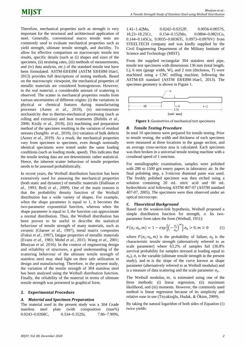
specimen geometry is shown in Figure 1.
Figure 1: Geometries of mechanical test specimens
B. Tensile Testing Procedure
In total 10 specimens were prepared for tensile testing. Prior
to tensile testing, the width and thickness of each specimen
were measured at three locations in the gauge section, and
an average cross-section area is calculated. Each specimen
was then broken in a universal tensile testing machine with a
crosshead speed of 1 mm/min.
For metallographic examination, samples were polished
with 280 to 1500 grit emery papers in laboratory air. In the
final polishing step, a 3-micron diamond paste was used.
The freshly polished specimen was then etched using a
solution containing 20 mL nitric acid and 60 mL
hydrochloric acid following ASTM 407-07 (ASTM standard
407-07, 2005). The specimens were then observed under an
optical microscope.
C. Theoretical Background
Based on the weakest-link hypothesis, Weibull proposed a
simple distribution function for strength, σ. Its two-
parameter form takes the form (Weibull, 1951):
𝐹(𝜎𝑖; 𝜎0, 𝑚) = 1 − 𝑒𝑥𝑝 [(−𝜎𝑖
𝜎0)
𝑚
] 𝜎0 > 0, 𝑚 > 0 (1)
where 𝐹(𝜎𝑖; 𝜎0, 𝑚) is the probability of failure, 𝜎0 is the
characteristic tensile strength (alternatively referred to as
scale parameter) where 63.2% of samples fail (36.8%
survival probability for samples stressed at loading equal to
𝜎0), 𝜎𝑖 is the variable (ultimate tensile strength in the present
study), and 𝑚 is the slope of the curve known as shape
parameter (alternatively referred to as Weibull modulus) and
is a measure of data scattering and the scale parameter 𝜎0.
The Weibull modulus, 𝑚 , is estimated using one of the
three methods: (i) linear regression, (ii) maximum
likelihood, and (iii) moments. However, the commonly used
method is linear regression because of its simplicity and
relative ease in use (Tiryakioǧlu, Hudak, & Ökten, 2009).
By taking the natural logarithm of both sides of Equation (1)
twice yields:

Bhuiyan et al.: A Tensile Strength Study of Stainless-Steel using Weibull Distribution
MIJST, Vol. 08, December 2020 3
𝑙𝑛 [𝑙𝑛 (1
1−𝐹(𝜎𝑖;𝜎𝑜,𝑚)] = 𝑚𝑙𝑛(𝜎𝑖) − 𝑚𝑙𝑛(𝜎𝑜) = 𝑚𝑥 + 𝑐 (2)
In Weibull statistics, the following four probability
estimators are commonly used (Bergman, 1984; Datsiou et
al., 2018):
𝐹(𝜎𝑖; 𝜎0, 𝑚) =𝑖
𝑛+1 (3a)
𝐹(𝜎𝑖; 𝜎0, 𝑚) =𝑖−0.5
𝑛 (3b)
𝐹(𝜎𝑖; 𝜎0, 𝑚) =𝑖−0.3
𝑛+0.4 (3c)
𝐹(𝜎𝑖; 𝜎0, 𝑚) =𝑖−0.375
𝑛+0.25 (3d)
where 𝑖 is the index of the ascending, 𝑛 is the sample size
(10 in the present study).
Bergman (1984) reported that probability estimators given
by Equation (3d) should be used for a small sample size
( 𝑛 < 20 ). Therefore, in the present study, probability
estimators defined by Equation (3d) is used to assign a
probability of failure to each ultimate tensile strength data
point.
The Weibull modulus, 𝑚 , and the characteristic tensile
strength, 𝜎0 , can be obtained by plotting
𝑙𝑛 [𝑙𝑛 (1
1−𝐹(𝜎𝑖;𝜎𝑜,𝑚)] against 𝑙𝑛(𝜎𝑖) . After taking a linear
regression of the data point, the slope of the regressed line is
the Weibull modulus, 𝑚, and the intercept is 𝑚𝑙𝑛(𝜎𝑜).
By fitting a straight line or applying the least square method
to 𝑙𝑛 [𝑙𝑛 (1
1−𝐹(𝜎𝑖;𝜎𝑜,𝑚)] as a function of 𝑙𝑛(𝜎𝑖), the Weibull
modulus 𝑚 is the slope and the scaling parameter or
characteristic tensile strength can be determined from the
intercept.
3. RESULTS AND DISCUSSION
A. General Mechanical Properties
Figure 2 shows the optical microstructure for the material
used in this study. A typical step structure is observed. C. A.
Della-Rovere et al. (2013) and A Bahrami et. al. (2019) also
reported similar microstructures of 304-grade stainless steel.
As reported earlier that in total ten tensile tests were
performed and corresponding ten stress-strain curves were
recorded for each material. A typical stress-strain curve is
shown in Figure 3. It is found that the tensile strength ranges
from 878 MPa to 1006 MPa, inferring that the ultimate
tensile strength appears to vary from specimen to specimen.
Table 1 and Table 2 lists the basic statistical properties of
ultimate tensile strength and yield strength of the material
used in this study. Note that the coefficient of variation
(COV = Standard Deviation (𝜎)/Mean (𝜇)100) is about
4.3% for ultimate tensile strength, and 7.6% for yield
strength. Kweon et al. (2020) reported that the ultimate
tensile strength of 304 stainless steel is in the range of 579 to
750 MPa. But our investigated material showed about 1.75-
1.90 times higher value of ultimate tensile strength that was
reported by Kweon et al. (2020). The observed difference
might have resulted due to random experimental errors such
as variation in width and thickness in the gauge section,
machining of specimen resulting in the variation of residual
stresses, microstructural heterogeneity in the gauge section.
Since the specimens were prepared using a CNC milling
machine, hence all the specimens used in this study were
identical in shape and size. Therefore, it is reasonable to
assume that the variation of width and thickness in the
specimen’s gauge section does not influence the observed
high value of ultimate tensile. It is well established that
during machining because of tool-material interactions, the
generated surface is affected through roughness, hardness,
residual stress distribution and thereby, influence the
mechanical properties of the manufactured parts (Kumar et
al., 2017; Ben Fredj et al., 2006; Gürbüz et al., 2017; Ma et
al., 2018). H. Sutanto (2007) investigated the characteristics
of residual stresses during CNC milling machining and
observed that very high compressive residual stress (−375
MPa) was induced at the surface of the work material. H. H.
Zeng et al. (2017) investigated the residual stresses in micro-
end milling considering sequential cuts effect and found
compressive residual stresses were induced by milling
operations. Therefore, based on the above discussion, it is
speculated that compressive residual stresses were also
induced during the CNC milling machining. However, the
surface residual stress is not measured in the present study.
Hence, it can be inferred that both microstructural
heterogeneity and the milling machining induced high
compressive residual stresses resulted in higher ultimate
tensile strength (about 1.75-1.90 times) in the studied
material. Furthermore, for precise and accurate
characterization of tensile properties, it is instructive to use a
more advanced technique such as electro-discharge
machining (EDM) for specimen preparation.
Table 1 Statistical Properties of the Ultimate Tensile Strength
Mean value (MPa)
Standard deviation (MPa)
Coefficient of variation (CV)
941 40.4 4.3%
Table 2 Statistical Properties of The Yield Strength
Mean value (MPa)
Standard deviation (MPa)
Coefficient of variation (CV)
577 44 7.6%
Figure 2: Optical microstructure of 304 stainless steel
Bhuiyan et al.: A Tensile Strength Study of Stainless-Steel using Weibull Distribution
MIJST, Vol. 08, December 2020 4
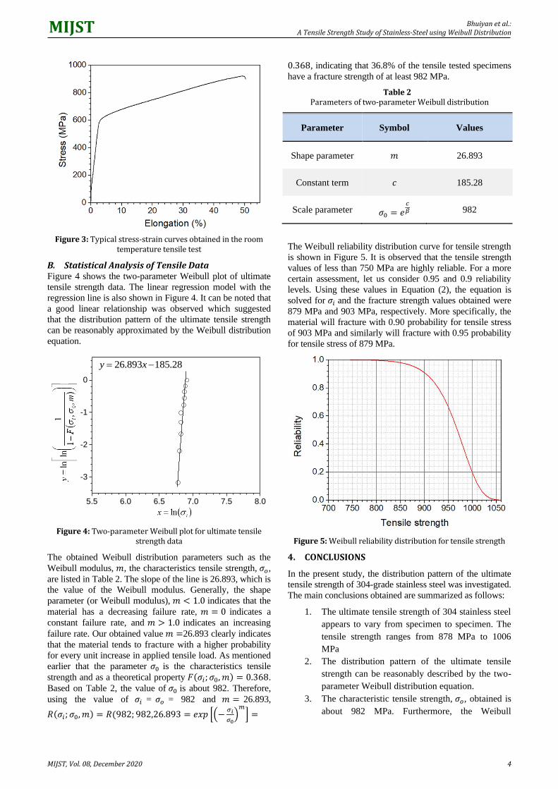
Figure 3: Typical stress-strain curves obtained in the room temperature tensile test
B. Statistical Analysis of Tensile Data
Figure 4 shows the two-parameter Weibull plot of ultimate
tensile strength data. The linear regression model with the
regression line is also shown in Figure 4. It can be noted that
a good linear relationship was observed which suggested
that the distribution pattern of the ultimate tensile strength
can be reasonably approximated by the Weibull distribution
equation.
Figure 4: Two-parameter Weibull plot for ultimate tensile strength data
The obtained Weibull distribution parameters such as the
Weibull modulus, 𝑚, the characteristics tensile strength, 𝜎𝑜,
are listed in Table 2. The slope of the line is 26.893, which is
the value of the Weibull modulus. Generally, the shape
parameter (or Weibull modulus), 𝑚 < 1.0 indicates that the
material has a decreasing failure rate, 𝑚 = 0 indicates a
constant failure rate, and 𝑚 > 1.0 indicates an increasing
failure rate. Our obtained value 𝑚 =26.893 clearly indicates
that the material tends to fracture with a higher probability
for every unit increase in applied tensile load. As mentioned
earlier that the parameter 𝜎0 is the characteristics tensile
strength and as a theoretical property 𝐹(𝜎𝑖; 𝜎0, 𝑚) = 0.368.
Based on Table 2, the value of 𝜎0 is about 982. Therefore,
using the value of 𝜎𝑖 = 𝜎𝑜 = 982 and 𝑚 = 26.893,
𝑅(𝜎𝑖; 𝜎0, 𝑚) = 𝑅(982; 982,26.893 = 𝑒𝑥𝑝 [(−𝜎𝑖
𝜎0)
𝑚
] =
0.368, indicating that 36.8% of the tensile tested specimens
have a fracture strength of at least 982 MPa.
Table 2 Parameters of two-parameter Weibull distribution
Parameter Symbol Values
Shape parameter 𝑚 26.893
Constant term 𝑐 185.28
Scale parameter 𝜎0 = 𝑒𝑐𝛽 982
The Weibull reliability distribution curve for tensile strength
is shown in Figure 5. It is observed that the tensile strength
values of less than 750 MPa are highly reliable. For a more
certain assessment, let us consider 0.95 and 0.9 reliability
levels. Using these values in Equation (2), the equation is
solved for 𝜎𝑖 and the fracture strength values obtained were
879 MPa and 903 MPa, respectively. More specifically, the
material will fracture with 0.90 probability for tensile stress
of 903 MPa and similarly will fracture with 0.95 probability
for tensile stress of 879 MPa.
Figure 5: Weibull reliability distribution for tensile strength
4. CONCLUSIONS
In the present study, the distribution pattern of the ultimate
tensile strength of 304-grade stainless steel was investigated.
The main conclusions obtained are summarized as follows:
1. The ultimate tensile strength of 304 stainless steel
appears to vary from specimen to specimen. The
tensile strength ranges from 878 MPa to 1006
MPa
2. The distribution pattern of the ultimate tensile
strength can be reasonably described by the two-
parameter Weibull distribution equation.
3. The characteristic tensile strength, 𝜎𝑜, obtained is
about 982 MPa. Furthermore, the Weibull
5.5 6.0 6.5 7.0 7.5 8.0
-3
-2
-1
0
28.185893.26 −= xy

Bhuiyan et al.: A Tensile Strength Study of Stainless-Steel using Weibull Distribution
MIJST, Vol. 08, December 2020 5
modulus (𝑚) for the investigated material is found
to be 26.893 inferring that the materials tend to
fracture with a higher probability for every unit
increase in applied tensile load.
4. The fracture statistics of the stainless steel were
examined by plotting the survival probability of
the specimen against the stress applied to the
specimen. It has been observed that the
relationship between the survival probability and
the applied stresses can be described by the
Weibull model. It also provides design engineers
with a tool that will help them to present the
necessary mechanical properties with confidence.
For example, with a 0.90 reliability level, it was
observed that the tensile strength of the present
material will be 903 MPa.
5. The varying tensile strengths of stainless steel are
due to their inherent internal structures, inferring
that there is no specific strength value to represent
mechanical behaviour. This study undoubtedly
raises questions of assuming the tensile strength
as an average of the experimental results.
Therefore, the distribution and reliability of
mechanical properties especially tensile strength
must be described by the probability of function
for their safe utilization in design and
manufacturing.
ACKNOWLEDGEMENTS
The authors would like to thank the Civil Engineering
Department, Military Institute of Science and Technology
(MIST) and STEELTECH Company for supplying the 304-
grade stainless steel material. The expert assistance by the
technical staff in the Civil Engineering department for
conducting the tensile test and the Mechanical Engineering
department for preparing the specimen at MIST is also
sincerely appreciated.
REFERENCES
Aksel, H., & Eren, O. (2015). A Discussion on the Advantages of
Steel Structures in the Context of Sustainable Construction.
New Arch-International Journal of Contemporary
Architecture, 2(3), 46–53.
https://doi.org/10.14621/tna.20150405
ASTM standard 407-07. (2005). ASTM 407-07, Standard Practice
for Microetching Metals and Alloys, ASTM International,
West Conshohocken, PA, 2007, 1–21.
https://doi.org/10.1520/E0407-07.2
ASTM E8/E8M-16ae1. (2013). Standard Test Methods for Tension
Testing of Metallic Materials. ASTM International, 1–27.
(Extracted on Dec. 02, 2020). Source:
http://www.astm.org/Standards/E8.htm
Azeez, S., Mashinini, M., & Akinlabi, E. (2019). Road map to
sustainability of friction stir welded Al-Si-Mg joints using
bivariate weibull analysis. Procedia Manufacturing, 33, 35–
42. https://doi.org/10.1016/j.promfg.2019.04.006
Bahrami, A., & Taheri, P. (2019). A Study on the Failure of AISI
304 Stainless Steel, 1–7.
Bedi, R., & Chandra, R. (2009). Fatigue-life distributions and
failure probability for glass-fiber reinforced polymeric
composites. Special Issue on the 12th European Conference
on Composite Materials, ECCM 2006, 69(9), 1381–1387.
https://doi.org/10.1016/j.compscitech.2008.09.016
Ben Fredj, N., Sidhom, H., & Braham, C. (2006). Ground surface
improvement of the austenitic stainless steel AISI 304 using
cryogenic cooling. Surface and Coatings Technology, 200(16–
17), 4846–4860.
https://doi.org/10.1016/j.surfcoat.2005.04.050
Bergman, B. (1984). On the estimation of the Weibull modulus.
Journal of Materials Science Letters, 3(8), 689–692.
https://doi.org/10.1007/BF00719924
Birbilis, N., Cavanaugh, M. K., & Buchheit, R. G. (2006).
Electrochemical behavior and localized corrosion associated
with Al7Cu2Fe particles in aluminum alloy 7075-T651.
Corrosion Science, 48(12), 4202–4215.
https://doi.org/10.1016/j.corsci.2006.02.007
Bony, S. Z., & Rahman, S. (2014). Practice of Real Estate Business
in Bangladesh: Prospects & Problems of High-rise building.
IOSR Journal of Business and Management, 16(7), 01–07.
https://doi.org/10.9790/487x-16740107
Chakma, J. (2019). Steel industry booming on mega projects.
(Extracted on Dec. 02, 2020). Source:
https://www.thedailystar.net/business/news/steel-industry-
booming-mega-projects-1735855
Datsiou, K. C., & Overend, M. (2018). Weibull parameter
estimation and goodness-of-fit for glass strength data.
Structural Safety, 73, 29–41.
https://doi.org/10.1016/j.strusafe.2018.02.002
Della-Rovere, C. A., Castro-Rebello, M., & Kuri, S. E. (2013).
Corrosion behavior analysis of an austenitic stainless steel
exposed to fire. Engineering Failure Analysis, 31, 40–47.
https://doi.org/10.1016/j.engfailanal.2013.01.044
Evans, A. G. (1983). Statistical aspects of cleavage fracture in steel.
Metallurgical Transactions A, 14(7), 1349–1355.
https://doi.org/10.1007/BF02664818
Feng, Q. B., Li, Y. B., Carlson, B. E., & Lai, X. M. (2019). Study
of resistance spot weldability of a new stainless steel. Science
and Technology of Welding and Joining, 24(2), 101–111.
https://doi.org/10.1080/13621718.2018.1491378
Fukui, Y., Yamanaka, N., & Enokida, Y. (1997). Bending strength
of an Al-Al3Ni functionally graded material. Composites Part
B: Engineering, 28(1–2), 37–43.
https://doi.org/10.1016/s1359-8368(96)00018-2
Glaeser, A. M. (1997). The use of transient FGM interlayers for
joining advanced ceramics. Composites Part B: Engineering,
28(1–2), 71–84. https://doi.org/10.1016/s1359-
8368(97)00039-5
Gürbüz, H., Şeker, U., & Kafkas, F. (2017). Investigation of effects
of cutting insert rake face forms on surface integrity.
International Journal of Advanced Manufacturing
Technology, 90(9–12), 3507–3522.
https://doi.org/10.1007/s00170-016-9652-7
Hallinan, A. J. (1993). A Review of the Weibull Distribution.
Journal of Quality Technology, 25(2), 85–93.
https://doi.org/10.1080/00224065.1993.11979431
Islam, F. A. S., Alam, M. M.. I., & Barua, S. (2016). Investigation
on the uses of steel as a sustainable construction material in
Bangladesh., International Journal of Scientific Engineering
and Applied Science (IJSEAS), 2(1), 41–52..
Islam, M. A. (2015). Corrosion behaviours of high strength TMT
steel bars for reinforcing cement concrete structures. Procedia
Engineering, 125, 623–630.
https://doi.org/10.1016/j.proeng.2015.11.084
Khatak, H. S., Gnanamoorthy, J. B., & Rodriguez, P. (1996).
Studies on the influence of metallurgical variables on the
stress corrosion behavior of AISI 304 stainless steel in sodium

Bhuiyan et al.: A Tensile Strength Study of Stainless-Steel using Weibull Distribution
MIJST, Vol. 08, December 2020 6
chloride solution using the fracture mechanics approach.
Metallurgical and Materials Transactions A: Physical
Metallurgy and Materials Science, 27(5), 1313–1325.
https://doi.org/10.1007/BF02649868
Király, M., Antók, D. M., Horváth, L., & Hózer, Z. (2018).
Evaluation of axial and tangential ultimate tensile strength of
zirconium cladding tubes. Nuclear Engineering and
Technology, 50(3), 425–431.
https://doi.org/10.1016/j.net.2018.01.002
Kumar, P. S., Acharyya, S. G., Rao, S. V. R., & Kapoor, K. (2017).
Distinguishing effect of buffing vs. grinding, milling and
turning operations on the chloride induced SCC susceptibility
of 304L austenitic stainless steel. Materials Science and
Engineering A, 687, 193–199.
https://doi.org/10.1016/j.msea.2017.01.079
Kweon, H. D, Kim, J. W., Song, O., & Oh, D. (2020).
Determination of true stress-strain curve of type 304 and 316
stainless steels using a typical tensile test and finite element
analysis. Nuclear Engineering and Technology, (in press).
https://doi.org/10.1016/j.net.2020.07.014
Ma, Y., Zhang, J., Feng, P., Yu, D., & Xu, C. (2018). Study on the
evolution of residual stress in successive machining process.
International Journal of Advanced Manufacturing
Technology, 96, 1025–1034. https://doi.org/10.1007/s00170-
017-1542-0
Mohd, S., Bhuiyan, M. S., Nie, D., Otsuka, Y., & Mutoh, Y.
(2015). Fatigue strength scatter characteristics of JIS SUS630
stainless steel with duplex S-N curve. International Journal of
Fatigue, 82, 371–378.
https://doi.org/10.1016/j.ijfatigue.2015.08.006
Monrrabal, G., Bautista, A., Guzman, S., Gutierrez, C., & Velasco,
F. (2019). Influence of the cold working induced martensite
on the electrochemical behavior of AISI 304 stainless steel
surfaces. Journal of Materials Research and Technology, 8(1),
1335–1346. https://doi.org/10.1016/j.jmrt.2018.10.004
Monteiro, S. N., Nascimento, L. F. C., Lima, É. P., Luz, F. S. da,
Lima, E. S., & Braga, F. de O. (2017). Strengthening of
stainless steel weldment by high temperature precipitation.
Journal of Materials Research and Technology, 6(4), 385–
389. https://doi.org/10.1016/j.jmrt.2017.09.001
Nur, S. A. (2016). Steel structures gaining popularity in cities.
(Extracted on Dec. 02, 2020). Source:
https://dailyasianage.com/news/28068/steel-structures-
gaining-popularity-in-cities
Rahman, M. (2019). Curbing air pollution. The Finincia Express.
(Extracted on Dec. 02, 2020). Source:
https://thefinancialexpress.com.bd/views/views/curbing-air-
pollution-1577111648
Sanaullah, M., Rahman, J., Ibrahim, I., & Rahman, M. S. (2019).
Behavior of Concrete Filled Stainless Steel Tubular Column
Under Axial Loads, MIST Journal of Science and Technology,
7(1), 9–18.
Sungho, P., Noseok, P., & Jaehoon, K. (2010). A statistical study
on tensile characteristics of stainless steel at elevated
temperatures. Journal of Physics: Conference Series, 240.
https://doi.org/10.1088/1742-6596/240/1/012083
Sutanto, H. (2007). Residual stresses on high-speed milling of
hardened steel using CBN cutting tool. Journal Tecknolgi of
Media Teknika, 7(2), 1-7.
Tiryakioǧlu, M., Hudak, D., & Ökten, G. (2009). On evaluating
Weibull fits to mechanical testing data. Materials Science and
Engineering A, 527, 397–399.
https://doi.org/10.1016/j.msea.2009.08.014
United Nations (2020). World Economic Situation and Prospects
2020. (Extracted on Dec. 02, 2020). Source:
https://www.un.org/development/desa/dpad/publication/world
-economic-situation-and-prospects-2020
Wang, H., Shi, Z., Yaer, X., Tong, Z., & Du, Z. (2019). High
mechanical performance of AISI304 stainless steel plate by
surface nanocrystallization and microstructural evolution
during the explosive impact treatment. Journal of Materials
Research and Technology, 8(1), 609–614.
https://doi.org/10.1016/j.jmrt.2018.05.010
Wang, Q. G., Apelian, D., & Lados, D. A. (2001). Fatigue behavior
of A356-T6 aluminum cast alloys. Part I. Effect of casting
defects. Journal of Light Metals, 1(1), 73–84.
https://doi.org/10.1016/S1471-5317(00)00008-0
Weibull, W. (1951). A Statistical Distribution Function of Wide
Applicability. Journal of Applied Mechanics, 18, 293–297.
Zeng, H. H., Yan, R., Peng, F. Y., Zhou, L., & Deng, B. (2017). An
investigation of residual stresses in micro-end-milling
considering sequential cuts effect. International Journal of
Advanced Manufacturing Technology, 91, 3619–3634.
https://doi.org/10.1007/s00170-017-0088-5
MIJST MIST International Journal of Science and Technology
MIJST, Vol. 08, December 2020 | https://doi.org/10.47981/j.mijst.08(02)2020.214(07-13) 7
Experimental Analysis on Safety System of a Simulated Small Scale Pressurized Water Reactor System with Intelligent Control
Md. Shakerul Islam, Altab Hossain*, Khalid Mursed, and Rafi Alam Chowdhury
Department of Nuclear Science and Engineering, Military Institute of Science and Technology (MIST), Dhaka, Bangladesh
emails: [email protected]; *[email protected]; [email protected]; and [email protected]
A R T I C L E I N F O
A B S T R A C T
Article History: Received: 14th April 2020 Revised: 17th June 2020 Accepted: 05th August 2020 Published: 16th December 2020
Reactors are widely used in the nuclear power plant due to the rapid demand for electricity by reducing the greenhouse effect. However, the effectiveness of the nuclear reactor depends on an adequate safety system. Hence, temperature and heat transfer are two critical parameters for any reactor in operation for which intelligent temperature control with an integrated safety system is essential. Therefore, the present study has emphasized the development of a simulated small-scale water-based reactor with intelligent control and safety system and examined through the analysis of thermal-hydraulic parameters. Radial heat transfer of an electric rod used as fuel in the primary circuit has been analyzed by taking sensor reading in various positions of the core. The developed system is self-controlled with all possible active and passive safety systems. Consecutively, the prototype has also been designed including manual adjustment to ensure a fail-safe environment. The system is capable to operate at temperatures between 80°𝐶 and 120°𝐶, although the design can withstand up to 200°𝐶. The data of the experiment are taken under the pressure of 200 𝑘𝑃𝑎 at 120°𝐶 temperature. Results show that heat output of 2116.09 𝑘𝐽 has been obtained from the system against heat input of 2514.80 𝑘𝐽, which gives an efficiency around 16% of the developed system.
Keywords:
Water-based reactor Intelligent control Thermal hydraulic Heat transfer Safety
© 2020 MIJST. All rights reserved.
1. INTRODUCTION
Fossil fuels used in conventional thermal power plants
cause many environmental problems. But nuclear energy
does not emit greenhouse gases unlike coal and natural gas
and hence, they do not contribute to climate change.
Since the world tries to reduce global warming, nuclear
power plant (NPP) is contributing to the energy mix by
generating a significant amount of electricity. In an
increasingly carbon-constrained future, nuclear power is
becoming recognized as an integral part of the world’s
low-carbon energy solution (Ho et al., 2019). Nuclear
power has grown quickly in the 1970s and 1980s, reaching
a global installed capacity of 396 GWe today (IAEA,
2019). It is found that the annual load factor of nuclear power in China is about 90%, which is much higher than
those of coal-fired power, wind power, and solar power
(Zhen, 2016). It is noted that two types of light water
reactors namely Pressurized Water Reactor (PWR) and
Boiling Water Reactor (BWR), are commonly used in the
world’s nuclear power plants. However, one of the main
differences between PWR and BWR is in the steam
generation process. In general, PWR consisting of primary
and secondary water circuit produces steam indirectly,
whereas BWR consisting of a single water circuit produces
steam directly. More precisely, in a PWR, the coolant
being heat at high temperature using heat from the reactor
core is forced to maintain its liquid form under high
temperature due to high pressure. Subsequently, the heat
produced from the primary water circuit is further
transferred to the secondary circuit which turns into steam
and rotates the turbine, thereby, producing electricity. On
the other hand, in a BWR, steam produced directly by the
boiling of water coolant is detached using steam separators
placed above the reactor core, and thereby, rotating the
turbine. Research shows that about 80% of operated
nuclear power plants are of PWR and BWR typed light
water reactor (Breeze et al., 2014). Ordinary water is used
as coolant and moderator in BWR typed reactor in which,
water is being boiled at the boiling point of 285°C at a
pressure of 7.5 MPa, and the steam generated is used
Islam et al.: Experimental Analysis on Safety System of a Simulated Small Scale Pressurized Water Reactor System with Intelligent Control
MIJST, Vol. 08, December 2020 8
directly to operate a steam turbine. However, the accident
at Three Mile Island (TMI) has led to an essential
improvement in the safety of nuclear plants throughout the
world. The investigation shows that the human element
had not been adequately included in previous safety
considerations, and this observation prompted numerous
advances in design and operating practices at nuclear
plants. Other notable changes in both hardware and
practices were research stimulated by accident (Kojima et
al., 2007). Nuclear power generated through a controlled
chain reaction is controlled through the four-factor formula
(P´al & P´azsit, 2009). If the reaction cannot be controlled,
then there is a possible chance of occurring major anomaly.
After the Chernobyl accident in 1986, the importance of
containment for severer accidents became highlighted
(Balonov, 2013). The reactor core was partially melted
down, thereby, many radioisotopes was released as the
consequence of the accident and many people were
evacuated from the exclusion zone (Miller, 1994). Again,
the nuclear accident that occurred in Fukushima Daiichi in
Japan was mainly caused by a massive tsunami which
made the station completely blackout (Khan et al., 2018).
Accident management was practiced both at Three Mile
Island and Chernobyl, with significant consequences in
both cases. The investigation of the TMI and Chernobyl
accident has shown the failure of the management
processes which are supposed to have an adequate safety
culture. In both cases, there were weaknesses in design,
operating practices, training, and feedback of operating
information, and there was no organized mechanism to
ensure that weaknesses were recognized and corrected.
The rate of civil nuclear accidents over time since 1952 has
been decreased significantly from the 1970s, reaching to be
a stable level of around 0.003 events per plant per year
(Wheatley et al., 2016). After Fukushima nuclear accident
in Japan, the elements such as transparency, acceptability
and communication capacity of nuclear safety information
have emerged as an important part of key elements for
nuclear safety regulation since 2010 (Kim et al., 2019).
The Chernobyl accident has led the International Safety
Advisory Group (INSAG) to accelerate the preparation of
INSAG-3. From all the accidents, one of the most
important lessons has been learned that the control system
of any reactor must be robust, efficient, and reliable at the
same time. Several studies have been performed on nuclear
reactor to ensure adequate safety, temperature control with
an integrated safety system (Gharib et al., 2011; Hossain et
al., 2019; IAEA, 2002; Khan & Islam, 2019; Sunday et al.,
2013; Vojackova et al., 2017; Nain et al., 2019). The
literature shows that the thermal-hydraulic models through
hot channel fuel centreline temperature play a significant
role to safety-related parameters within the design limit
(Rahman et al, 2014). However, the investigation was
performed using computer code and the data were far to
compromise the safety of the reactor. Hence, experimental,
and theoretical studies on heat transfer, intelligent control
and safety system are very important for any nuclear
reactor. Moreover, it is found that experimental studies are
important for making a relationship between the flow rate
and electrical power of the motor driving the pumps which
must be addressed in a nuclear reactor. Therefore, this
study has been performed with the development of a
simulated small-scale water based PWR reactor.
Furthermore, the analysis has been carried out to evaluate
the heat transfer, safety, and control system of a working
reactor model.
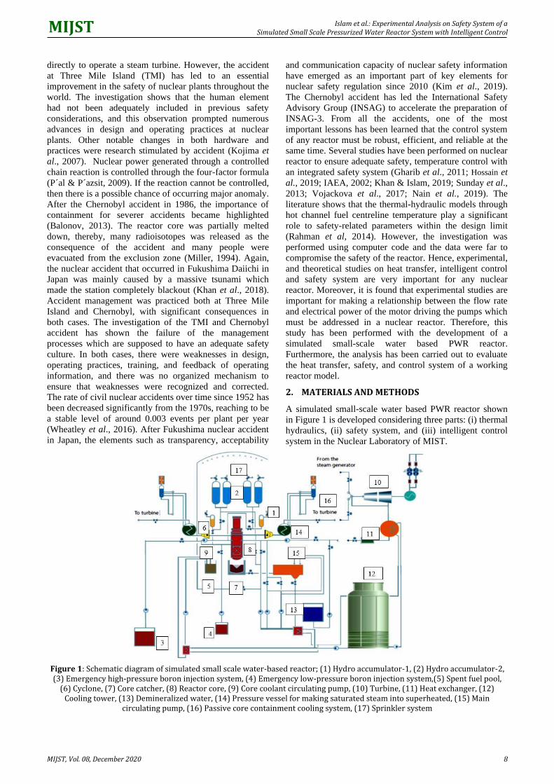
2. MATERIALS AND METHODS
A simulated small-scale water based PWR reactor shown
in Figure 1 is developed considering three parts: (i) thermal
hydraulics, (ii) safety system, and (iii) intelligent control
system in the Nuclear Laboratory of MIST.
Figure 1: Schematic diagram of simulated small scale water-based reactor; (1) Hydro accumulator-1, (2) Hydro accumulator-2, (3) Emergency high-pressure boron injection system, (4) Emergency low-pressure boron injection system,(5) Spent fuel pool,
(6) Cyclone, (7) Core catcher, (8) Reactor core, (9) Core coolant circulating pump, (10) Turbine, (11) Heat exchanger, (12) Cooling tower, (13) Demineralized water, (14) Pressure vessel for making saturated steam into superheated, (15) Main
circulating pump, (16) Passive core containment cooling system, (17) Sprinkler system

Islam et al.: Experimental Analysis on Safety System of a Simulated Small Scale Pressurized Water Reactor System with Intelligent Control
MIJST, Vol. 08, December 2020 9
Table 1 Key Output Parameters
Parameter Symbol Value Unit
Heat input qin 2514.80 kJ/kg
Heat output qout 2116.09 kJ/kg
Net work Wnet 398.71 kJ/kg
Thermal Efficiency η 0.16 16%
The mass flow rate of steam ṁ 0.00376 kg/s
Rate of Heat Rejection in Cooling Water 0
Qout 7.96 kJ/s
The mass flow rate of cooling water from
the cooling tower ṁcooling water 0.33 kg/s
Temperature difference at the cooling water
inlet and outlet ∆Tcooling water 5.68 °C
The heat is first generated in the core and then it heats the
water, which goes to the steam generator and generates
steam. The produced steam is then transferred to the
turbine to rotate and thereby, producing electricity through
a generator. After rotating the turbine shaft, the waste heat
goes to a heat exchanger by cooling down with the help of
the cooling tower. Consecutively, with the help of the
distillation again the cooled water goes back to the core.
A. Design Parameter Optimization A thermal-hydraulic study has been performed in this work
by considering temperature, amount of heat generation,
amount of heat release, and flow measurement. Heat
transfer used in this study using conduction and convection
laws of the heating rod to cladding surface followed by
coolant are shown in Equations (1) and (2).
2 1( )Q kA T T
t d
−= (1)
where, Q is the heat transfer, t is the time, k is the thermal
conductivity of the material, T2 and T1 are the temperatures
of corresponding material at the inner and outer surface,
and d is the thickness of the material.
( )sc aq h A T T= − (2)
where, q is heat transfer per unit time, A is heat transfer
area, hc is convective heat transfer coefficient Ts is surface
temperature and Ta is coolant temperature. However, one of
the important factors of the NPP life cycle is the condition of
the reactor pressure vessel (RPV) and its fatigue life. The
stainless steel used in this study has been investigated with
DPA effect at 823 K temperature to a neutron fluence of
1×1025n/m2 (Ioka et. al, 2000). DPA generally is defined as
displacement per atom is employed to normalize the
radiation damage across the reactor containment. Equation
(3) is used in this study to determine the thickness of the
reactor containment material made of stainless steel.
2 0.2
i i
i
P Dt
SE P=
− (3)
where, Pi is the internal pressure of the containment, Di is
the internal diameter of the containment, S is allowable
stress, E is the joint efficiency and t is the material
thickness. An ellipsoidal head is chosen with a thickness of
4.053 mm by using Eq. (3) which is the same as the hoop
stress thickness of
the reactor pressure vessel. Since the minimum thickness
of the wall chosen is 7 mm, the head thickness of 7 mm is
adequate in this work. Table 1 represents the optimized
parameters for developing the small-scale water-based
reactor.
B. Development of Physical Model The reactor core is divided into two parts- the lower half
and the upper half along with an instrumentation channel.
The instrumentation channel holds all the thermocouples.
The body of the reactor core is constructed with stainless
steel consisting of alloy composition of 17-20% Cr, 8-12%
Ni, and 2% Mo to mitigate the corrosion. The upper half of
the reactor core is made with glass to observe the thermal-
hydraulic properties as well as steam separators. Three
flow sensors have been used to measure the flow rate at the
inlet and outlet. Basically, they send signals based on the
amount of coolant flow. Then the recorded signals are
multiplied with the necessary co-efficient to get the exact
result. Two pressure sensors have also been used. Two
types of safety systems have been utilized in the model: (i)
active safety systems, and (ii) passive safety systems. Most
of them are worked by a pulse feedback method here.
Emergency Core Cooling System (ECCS) with high-
pressure injection and low power injection module is
included in the model. Both have a self-start-up algorithm
means that they can work without any human interference.
The sprinkler system of the containment is also included in
the model which has a total of three stages. Each of the
stages contains two sets of the sprinkler system. The whole
containment is covered with a total number of six
sprinklers. For station blackout, a gravity-driven water
supply system is included in the model. It is basically
worked by an electromagnet. When station blackout occurs,
the electromagnet is demagnetized letting the water flow in
the reactor core. Furthermore, an online passive air-cooling
system is also integrated into the model. If all electrical
components are failed, then the water from the hydro-
accumulator is automatically processed to flood the core.

Islam et al.: Experimental Analysis on Safety System of a Simulated Small Scale Pressurized Water Reactor System with Intelligent Control
MIJST, Vol. 08, December 2020 10
Each container is filled with 5 liters of water with a flowing
rate of 0.3 liters per minute. The heat exchanger used in this
study is shell and core type and consisted of sixteen ‘U’
loops. A four-stage water filtration system and two-stage
containment air filtration systems have also been used in
this model.
C. Development of Control System An intelligent control system has been developed by using
Microsoft visual basic for controlling the whole system.
The code has been developed in the .Net platform. Figure 2
shows the power control flow chart of the overall system.
From the figure, it is revealed that the thermocouple starts
to measure the temperature after the initiation of the
system. Based on the temperature obtained from the
experiments, the thermocouple sends a signal to the
microcontroller. The microcontroller compares the signal
as per set temperature. If the reading matches well then it
sends a signal to the controller unit so that the controller
unit can readjust the power to maintain the stabilization of
the system. Besides the code, all the microcontrollers are
programmed with a self-maintained algorithm, from which
most of them are PID based. With the help of an
electromagnetic relay and using a variable resistor, the
power can be controlled from the developed software by
using a microcontroller.
Figure 3 shows the power control circuit of the overall
system. With the help of a thermocouple, water level
sensor, and pressure sensor, the condition of the reactor
core is maintained by the microcontroller. Arduino Mega
(Mega 2560, 16 MHz) is used for the experiment. This
microcontroller is well known for its reliability along with
54 digital output, 15 analog input and 15 analog output.
The microcontroller used in this study has two pulses with
a time duration of 3 seconds. If any transient situation
occurs, the sensors send the values which are not the same
as setpoint values. If only a single pulse comes, the
microcontroller considers it as a false count. If the second
abnormal pulse is found, then the microcontroller starts the
ECCS to maintain the setpoint values, which is
programmed using the PID algorithm. If the reactor core
pressure rises from a certain level, the high-pressure
injection system starts automatically. In this study, K-type
(MAX6675) thermocouple is used in the model to achieve
the temperature of the heat source. Out of a total of 16
sensors, only 8 sensors are used to take the reading from
the reactor core. The readings obtained using sensors are
the axial and radial temperature of the core. The
thermocouples are calibrated with a mechanical
thermometer to get accurate results. Besides, the readings
from the thermocouples are directly obtained at a computer
monitor where I2C LED (32 bit) monitors are used for
getting the same result for the redundancy. An advanced
code is developed along with an advanced algorithm based
on If-Else (Patnaikuni, 2017). Initially, thermocouples take
data from the reactor core and then signals are sent to the
microcontroller. Microcontroller analyzes these data,
whether they are true or false. If the data are true, then they
are displayed on the monitor. If false, then the
microcontroller sends back the signal to the source.
Besides the core, another 8 thermocouples are used to
measure the temperature at the inlet, outlet, turbine,
condenser, and cooling tower. Two pressure meters are
used to take the pressure data from the core. Furthermore,
an air quality sensor is used to analyze the quality of air.
Also, several types of active and passive safety systems are
included in the study. Most of them are worked by a pulse
feedback method.
Figure 2: Power control flow chart of the overall system
Figure 3: Circuit of control system; (1) Microcontroller, (2) Relay Module
Figure 4 shows the arrangement of thermocouples and heat
generation source. Another three of them remain
disconnected as back up. Three rows of thermocouples (80
mm distance) are installed in the core for taking axial and
radial temperature distribution. Each row contains three
thermocouples of which two are used to take radial
temperature, and one is used to take the axial temperature.
The mass flow rate of steam is considered as 0.00376 kg/s
in this study. Since the mass flow rate of steam is very
small, the turbine is made as very light weighted. YF-S201
(hall-effect, 15ma-5v) flow sensor is used in this study.
Similarly, the network is calculated as 398.70 kJ/kg and
thereby producing thermal power of 1500 W.

Islam et al.: Experimental Analysis on Safety System of a Simulated Small Scale Pressurized Water Reactor System with Intelligent Control
MIJST, Vol. 08, December 2020 11
Figure 5 shows the lower half of the core with the
instrumentation channel. The instrumentation channel
holds all the thermocouple. The body of the core is
constructed with stainless still to mitigate the corrosion.
Figure 6 shows the upper half of the core, which is made
with glass to observe the thermal-hydraulic properties as
well as steam separator. Three flow sensors have been used
to measure the flow rate of inlet and outlet for sending
analog signals based on the amount of coolant flow. Two
pressure sensors have been used to measure the flow rate
of inlet and outlet for sending analog signals based on the
amount of coolant flow. Six coils are installed for heat
generation. Each of them has a 500W capacity. Three of
them are in the operational phase for fulfilling the energy
supply for the whole system. Figure 7 shows the setup of
the developed model. High-pressure injection and low-
pressure injection systems work in the same procedure.
The only difference from ECCS is that they also take
pressure into consideration. Besides, the ECCS and
containment spray system and online air filtration system
are also included in the model project. The main
circulations pump works based on the core temperature.
The speed of the pump varies with increasing or decreasing
core temperature. The microcontroller takes the
temperature data from the core. Then based on the
temperature data, it sets the speed of the motor which, is
executed by the PWM signal sent to the pump control
driver.
Figure 4: Thermocouple and heat source in the core; (1) Thermocouple, (2) Heat source
Figure 5: Instrumentation channel and core
Figure 6: Final setup of the developed model
Figure 7: Final setup of the developed model; (1) Core, (2) Heat exchanger, (3) Control system, (4) Heating rod indicator, (5) Distillation and water purification, (6) Hydro accumulator,
(7) Display board
3. RESULTS AND DISCUSSION
The results obtained from the experimental setup are
recorded and plotted in a graphical system. Figure 8 shows
the axial and radial temperature distribution over time. The
x-axis is denoted as time in s while the y-axis is represented
as the temperature in ℃. The blue line represents the axial
temperature with thirty seconds time duration while the
green line represents the radial temperature distribution.
Figure 8 reveals that the axial and radial temperatures
begin to decrease after the creation of an anomaly
situation. Figure 9 shows the steam flow rate and water
inlet flow rate in kg/s in comparison with time in s. A
thirty-second time interval is considered for recording data.
The blue line indicates the steam flow rate, and the red line
indicates the water inlet flow rate. The x-axis is denoted as
time, and the y-axis is denoted as a flow rate. Besides, all
the safety system works well while operating the system.
However, to evaluate the safety system of the model, an
anomaly of small break LOCA has been made manually.
Figure 10 represents the relationship between the flow rate
of ECCS and the reduction of core temperature with time.
It is noticed that the activation of ECCS starts
automatically after crossing the core temperature of 97°C
at atmospheric pressure. According to Westinghouse
Technology, the ECCS charging rate is 150 gpm. The
ECCS is designed by scaling in such a way that it can

Islam et al.: Experimental Analysis on Safety System of a Simulated Small Scale Pressurized Water Reactor System with Intelligent Control
MIJST, Vol. 08, December 2020 12
supply a maximum of 5 L of water per minute, i.e., 0.087
kg/s to the core. The transient situation has been made after
the functional operation of the reactor with a period of 210
seconds. From Figure 10, it has been observed that the
ECCS flow rate is stable during 0 to 210 seconds and no
transient situation occurred. However, a transient situation
occurred after 210 seconds where the temperature of the
core increases suddenly and thereby, starting ECCS. ECCS
has been deactivated after 420 seconds as the temperature
is decreased and reached under a margin of safety.
Similarly, the reduction of decay heat based on the
temperature in comparison with time plays an important
role. It is noticed that the temperature has increased
quickly and reached a peak during the transient period of
210 s to 420 s. At this stage, the safety system has been
started to work and hence the temperature is decreased
which represents the reduction of decay heat.
Figure 8: Temperature distribution versus time
Figure 9: Flow rate of steam and water inlet versus time
Figure 10: Graphical relationship between the flow rate of ECCS and reduction of core temperature with time
Figure 11 represents the reduction of power load based on
the temperature in comparison with time. Surprisingly, the
reactor has tripped with the decrease of temperature
drastically as the result of transient which results in the
reduction of net power. Subsequently, the power is reached
to the minimum value, i.e., 0 after 600 s and thereby,
reducing power. From Figure 11 it is seen that power
decreases gradually from 210 to 600 seconds
Figure 11: Graphical representation of the power load reduction versus time
after the reactor trip. On the other hand, humidity has been
found at a satisfactory level. The reason behind this is that
the online water purification and containment air-
purification systems work very swiftly. Not only this but
also a high-pressure injection system and a low-pressure
injection system work perfectly. The gravity-driven hydro
accumulator for station blackout also works perfectly
40
50
60
70
80
90
100
0 100 200 300 400 500 600 700
Tem
pe
ratu
re (
°C)
Time (s)
Axial
Radial
0
0.01
0.02
0.03
0.04
0.05
0 100 200 300 400 500 600
Flo
w R
ate
(kg
/s)
Time (s)
Steam Flow
Coolant Flow
-10
0
10
20
30
40
50
60
40
50
60
70
80
90
100
0 100 200 300 400 500 600 700
Flo
w R
ate
(kg
/s ×
10
-4)
Tem
pe
ratu
re (
°C)
Time (s)
Temperarture Flow rate
0
20
40
60
80
100
120
0 100 200 300 400 500 600 700
Po
we
r Lo
ad R
ed
uct
ion
(%
)
Time (s)

Islam et al.: Experimental Analysis on Safety System of a Simulated Small Scale Pressurized Water Reactor System with Intelligent Control
MIJST, Vol. 08, December 2020 13
supplying 2 𝐿 water during station blackout. The passive
heat removal system has been found as working perfectly.
4. CONCLUSIONS
The analysis has been performed to evaluate the thermal-
hydraulic properties of a working reactor model.
Theoretical calculations have been performed to construct
the reactor model and examine the effect of heat transfer.
Temperatures, flow rates, and pressures have been
considered as main thermal-hydraulic properties. It is
revealed that the system is capable to operate at
temperatures between 80°𝐶 and 120°𝐶 , although the
design can withstand up to 200°𝐶 . Similarly, the system
can withstand pressure up to 600 𝑘𝑃𝑎 though the working
pressure is not more than 500 𝑘𝑃𝑎 . The data of the
experiment are taken under the pressure of 200 𝑘𝑃𝑎 at
120°𝐶 temperature. However, error analysis has not been
done but data has been repeated six times for which almost
similar data has been obtained and found no significant
variation. The results show that a heat output of
2116.09 𝑘𝐽 has been obtained from the system against a
heat input of 2514.80 𝑘𝐽 , which gives a network of
398.71 𝑘𝐽 . Furthermore, the efficiency is found as
16% proving the effective performance of the developed
system. However, specific conclusions can be drawn from
the study are as follows:
1. The average axial and radial temperatures have
been found as 93℃ and 90℃ with 0.021 𝑘𝑔/𝑠
steam outlet and 0.045 𝑘𝑔/𝑠 water inlet.
2. 0.45 − 𝑤𝑎𝑡𝑡 power has been obtained against the
energy insertion of 400 joules at a pressure of
1.5 𝑎𝑡𝑚.
3. The developed intelligent control system is highly
stable.
ACKNOWLEDGEMENTS
The authors would like to thank the Military Institute of
Science and Technology (MIST) for providing financial
support and laboratory facilities.
REFERENCES
Balonov, M. (2013). The Chernobyl Accident as a Source of New
Radiological Knowledge: Implications for Fukushima
Rehabilitation and Research Programmes. Journal of
Radiological Protection, 33, 27-40.
Breeze, P. (2014). Nuclear power Generation Technologies,
Newnes Publication. 3rd Edition, Elsevier Ltd.
Gharib, M., Yaghooti, A. & Buygi, M. O. (2011). Efficiency
Upgrade in PWRs, Energy and Power Engineering, 3, 533-
536.
Ho, M., Obbard, E., Burr, P. A. & Yeoh, G. (2019). A Review on
the Development of Nuclear Power Reactors, Energy
Procedia, 160, 459-466.
Hossain, A., Islam, S., Hossain, T, Salahuddin, A. Z. M & Sarkar,
A. R. (2019). An Intelligent Approach for Thermal-Hydraulic
Studies on Safety and Efficiency of Nuclear Power Plant.
Energy Procedia, 160, 436-442.
IAEA (2002). Accident Analysis for Nuclear Power Plants. IAEA
Safety Reports Series No. 23, IAEA, Vienna.
IAEA (2019). Energy, Electricity and Nuclear Power Estimates for
the Period up to 2050. IAEA Reference Data Series No. 1.
2019 Edition, IAEA, Vienna.
Ioka, I., Yonekawa, M., Miwa, Y., Mimura, H., Tsuji, H. &
Hoshiya, T. (2000). Effect of Helium to dpa Ratio on Fatigue
Behavior of Austenitic Stainless Steel Irradiated to 2 dpa,
Journal of Nuclear Materials, 283-287, 440-445.
Khan, A. H., & Islam, M. S. (2019). Prediction of thermal
efficiency loss in nuclear power plants due to weather
conditions in tropical region, Energy Procedia, 160, 84-91.
Khan, A. H., Hasan, S. & Sarkar, M. A. R. (2018). Analysis of
Possible Causes of Fukushima Disaster, International Journal
of Nuclear and Quantum Engineering, 12(2), 53-58.
Kim, J. S., Park, S. Y. & Lee, D. H. (2019). Changes and Prospects
of Safety Regulation Activities in Korean Nuclear Safety
Research, International Journal of Innovative Technology and
Exploring Engineering, 8(852), 777-783.
Kojima, T. & Sato, Y. (2007). Variations of a Passive Safety
Containment for a BWR with Active and Passive Safety
Systems, Journal of Nuclear Engineering and Design, 237, 74-86.
Miller, K. L. (1994). The Nuclear Reactor Accident at Three Mile
Island, Radiographics, 14(1), 215-224.
Nain, H. M. Z., Islam, M. S. & Khan, A. H. (2019). A Study on
Thermal-Hydraulics Characteristics for Designing a Shell and
Tube Condenser for a 1200 MWe Nuclear Power Plant. J.
Bangladesh Acad. Sci. 43(2), 181-189.
P´al, L. & P´azsit, I. (2009). The Fast Fission Factor Revisited.
Nuclear Science and Engineering, 161(1), 111-118.
Patnaikuni, D. R. P. (2017). A Comparative Study of Arduino
Raspberry Pi and ESP8266 as IoT Development Board.
International Journal of Advanced Research in Computer
Science, 8(5), 2350-2352.
Rahman, M. M., Akond, M. A. R., Basher, M. K., & Huda, M. Q.
(2014). Steady-State Thermal-Hydraulic Analysis of TRIGA
Research Reactor, World Journal of Nuclear Science and
Technology, 4, 81-87.
Sunday, J. I., Daniel, R. E., & Okibe, A. E. (2013). Simulation of
Safety and Transient Analysis of a Pressurized Water Reactor
using the Personal Computer Transient Analyzer, Leonardo
Electronic Journal of Practices and Technology, 22, 93-105.
Vojackova, J., Novotny, F. & Katovsky, K. (2017). Safety
Analyses of Reactor VVER 1000, Energy Procedia, 127, 352-359.
Wheatley, S. Sovacool, B. K. & Sornette, D. (2016). Reassessing
the Safety of Nuclear Power. Energy Research & Social
Science, 206, 1-5.
Zhen, Y. Q. (2016). Safety and Effective Developing Nuclear
Power to Realize Green and Low-carbon Development.
Advances in Climate Change Research, 7(1–2), 10-16.

MIJST MIST International Journal of Science and Technology
MIJST, Vol. 08, December 2020 | https://doi.org/10.47981/j.mijst.08(02)2020.196(15-23) 15
Corrosion Behavior of Copper Based Heat Exchanger Tube in Waters of Bangladesh Region at Varied Temperature and Flow Velocity
M. Muzibur Rahman1* and S. Reaz Ahmed2
1 Department of Naval Architecture & Marine Engineering, Military Institute of Science and Technology, Dhaka, Bangladesh 2 Department of Mechanical Engineering, Bangladesh University of Engineering and Technology, Dhaka, Bangladesh
emails: 1*[email protected]; [email protected]
A R T I C L E I N F O
A B S T R A C T
Article History: Received: 30th April 2020 Revised: 06th June 2020 Accepted: 04th August 2020 Published: 16th December 2020
Heat exchangers used in the ships are mostly of water-cooled shell and tube type, whose tube stacks are made of copper-based materials due to the requirement of high corrosion resistance and high thermal conductivity. Even though, the copper made heat exchanger tubes do fail on board ships because of corrosion. More point of contention arises when it is manufactured by companies that have limited supporting data and documentations. In this context, the present paper investigates the corrosion behavior of copper tubes of heat exchanger to assess the life span of the tube stack for on-board applications. A series of experiments have been undertaken to investigate the corrosion rates of copper tubes in sea water and river water with flow velocity of 1.0 𝑚/𝑠, 1.5 𝑚/𝑠 and 2.0 𝑚/𝑠 for the tube side entry temperature of 20°𝐶. The same experiments have been repeated for the shell side temperatures of 20°𝐶, 40°𝐶, 60°𝐶 and 80°𝐶. The investigations have revealed that the corrosion in sea water is about three times higher than that of river water. The increases in temperature and flow velocity have increased the rate of corrosion to a significant level contributing to shorten the life span.
Keywords: Corrosion Copper tube Heat exchanger River vs sea water Life span estimation
© 2020 MIJST, All rights reserved.
1. INTRODUCTION
Copper is chosen for the tube stacks of heat exchanger due
to its superior thermo-mechanical properties such as
thermal conductivity, resistance to corrosion, strength, and
formability (Collini, 2012). It may be mentioned that
copper is located in the periodic table in line of noble
metals, and thus copper is considered as immune from
corrosion. The corrosion immunity of copper is also based
on a postulation on the existence of native copper in the
earth’s crust (Davis, 2001). In the atmosphere, a very thin
layer of brownish-green or greenish blue in color known as
patina is formed (Graedel et al., 1987; Leygraf et al.,
2019). Established patina becomes stable and remains as a
permanent part of the copper object in the atmosphere.
Examples of the corrosion resistance of copper materials
are artifacts that have been found in nearly pristine
condition after having been buried in the earth for
thousands of years, and copper roofing in rural atmosphere
has been found to corrode at rates of less than 0.4 mm in
200 years (Cramer & Covino, 2005, pp. 125). But, in
water, copper corrodes due to number of factors as
considered differently by different researchers (Hedin et
al., 2018; Hultquist et al., 2009, 2011 & 2015; Hultquist,
2015; Simpson & Schenk, 1987; Szakalos et al., 2007).
According to a group of researchers (Hultquist et al. 2015),
the oxygen is consumed through hydrogen-oxygen reaction
and the hydrogen is coming out from the reaction of
copper with water. It is considered that the hydrogen-
oxygen reaction is faster than the formation rate of the
initially atomic hydrogen from the corrosion reaction itself
on copper (Hultquist et al., 2015) and it is not possible to
detect the hydrogen released from copper if the supply rate
of oxygen to the surface exceeds the rate of hydrogen
generation; and copper is considered erroneously as
corrosion resistant (Hultquist et al. 2009 & 2011). On the
other hand, few researchers (Simpson & Schenk, 1987;
Hedin et al., 2018) have expressed the disagreement on the
corrosiveness of copper in pure water.
However, corrosion of copper in sea water is accepted by
all the mariners as well as researchers due to
aggressiveness of ingredients like dissolved oxygen,
chloride, sulphate, dissolved solids, suspended solids etc.

Rahman & Ahmed: Corrosion Behavior of Copper Based Heat Exchanger Tube in Waters of Bangladesh Region at Varied Temperature and Flow Velocity
MIJST, Vol. 08, December 2020 16
present in the sea water (Abdallah et al., 2009; Farro et al.,
2009; Francis, 2010; Gudas & Hack, 1979; Nunez et al.,
2005; Orozco-Cruz et al., 2017; Pehkonen et al., 2002;
Rahmanto et al., 2002; Schumacher, 1979; Zakowski et al.,
2014). Beside the aggressive ingredients, few dynamic
parameters such as velocity, pressure, temperature,
conductivity, pH value, etc. are playing some role in the
corrosion behavior of metal in contact with sea water
(Gerasimov & Rozenfeld, 1958; Kong et al., 2017;
Kristiansen, 1977; Lee et al., 2016; Mor & Beccaria, 1979;
Poulson, 1993; Roy et al., 2018; Sabri et al., 2012;
Utanohara & Murase, 2019; Wan et al., 2012; Yatsenko et
al., 1999). Moreover, various types of corrosion attacks
can occur to the marine equipment made up of copper
materials exposed to sea water. In view of above, the
corrosion behaviors of metals including copper coming in
contact with sea water especially during operations at
elevated temperature along with significant flow velocity
need to be characterized at specific water and environment
conditions to assess the performance of marine machinery
(Pehkonen et al., 2002).
Bangladesh being a maritime nation with long glory of
shipbuilding heritage must have development in marine
sector (Rahman, 2017). At the same time, a good number
of vessels are plying in the inland water ways and at the
coast of Bangladesh, which use river/sea water in heat
exchangers to cool fresh water and lubricating oil of
marine engines for propulsion and power generation. This
requirement pushes the stake holders to look for reference
data to have design allowances and life span assessment of
marine equipment especially the heat exchanger on the
issue of corrosion. But, unfortunately, necessary data for
making decisions based on experimental results on
corrosion are neither available to mariners nor even to
local shipbuilding industries. One of such cases is the
reliability problem due to absence of data of locally
manufactured shell and tube type heat exchanger having
copper tube stack.
At this juncture, it is very important to carry out the study
on characterization of corrosion behavior of materials
commonly used on board ships, which are especially
coming in contact of sea water so that the shipbuilding can
be enhanced as the real ‘thrust sector’ of national economic
progress with the implementation plan of sustainable
development goals (SDGs). To this effect, the present
work is an attempt to investigate the corrosion behavior of
locally made copper heat exchanger tubes to be used in the
inland river water as well as coastal sea water environment
of Bangladesh region.
2. MATERIALS AND EXPERIMENTAL DETAILS
To investigate the corrosion behavior of copper-based tube
stack of shell and tube type heat exchanger for onboard
ships with marine propulsion and power generation
engines, two bundles of copper tubes manufactured in a
local shipyard of Bangladesh for coastal vessels were
collected. Each tube was of 400 𝑚𝑚 length, 9.525 𝑚𝑚
outer diameter and 1.245 𝑚𝑚 (18 𝐵𝑊𝐺 ) wall thickness.
Before the corrosion testing experiments, the chemical
composition of the tube material was tested using XRF
machine (model: Olympus DPO-2000-CC having silicon
drift detector for element identification) and
microstructures were observed using computer interfaced
Optical Electronic Microscope (model: Nikon BW-S500
having 4.19 Mpixel camera). The chemical composition of
tube is found to be of 99.934% 𝐶𝑢 , 0.019% 𝑆𝑖 ,
0.016% 𝑃, 0.018% 𝐹𝑒, and 0.013% 𝑁𝑖.
The heat exchangers for ships are supposed to cool the
engine lubricating oil and jacket water through an engine
driven pump that supplies water from river or sea
according to the plying location of the ship. The designated
ship is designed to be operated from Khulna to Chittagong,
and thus the heat exchangers would use inland water near
Khulna area for river cruise as well as sea water during
crossing the Bay of Bengal up to Chittagong. Considering
the operational requirements of the ship, two identical
experimental set-up arrangements were prepared, i.e., one
for river water and another for sea water. Accordingly,
5000-liter water from each location, i.e., Rupsha River and
the Bay of Bengal was collected for the experimental
purpose. The laboratory test result of the collected water is
presented in Table 1.
Table I Contents and properties of water used for investigation
Parameter River
Water
Sea
Water
pH 7.08 7.14
Total Dissolved Solids (mg/liter) 250 28000
Total Suspended Solids (mg/liter) 15 48
Chloride (mg/liter) 4500 21000
Sulphate (mg/liter) -- 1320
Dissolved Oxygen (mg/liter) 6.55 7.29
Electric Conductivity (µS/cm) 450 48000
The components for each experimental set-up include
pumps, tanks, flexible pipes, fittings, manifold, heat
exchanger tubes, flow meter, thermometers, thermostat,
relay, electric heater, etc. The straight tubes were placed
with the removable headers and manifolds in the
experimental set-up to observe their corrosion behavior
using gravimetric method. The operating temperature of
the heat exchanger of a marine engine remains normally
from 45℃ to 75℃ on shell side for the temperature of
lubricating oil and jacket water due to variation of engine
load, and in the tube side, the cooling water temperature is
from 18℃ to 30℃ due to seasonal variation. Therefore,
experiments were carried out for the shell side
temperatures of 20℃ , 40℃ , 60℃ and 80℃ so that
corrosion behavior against these temperatures can be
obtained. For the experiment at 20℃, normal fresh water
was passed through the shell side, and for 40℃, 60℃, and
80℃ , hot water was circulated using electric heaters to
maintain the temperature during each experiment. The
cooling water was stored in the open type tank for natural
air cooling and an arrangement was made on the return line
of tube side cooling water to spray in the atmosphere for
maintaining the normal temperature. Both hot water and
cooling water were reused with closed circuit arrangements
as shown in Figure 1.

Rahman & Ahmed: Corrosion Behavior of Copper Based Heat Exchanger Tube in Waters of Bangladesh Region at Varied Temperature and Flow Velocity
MIJST, Vol. 08, December 2020 17
Figure 1: Layout of Experimental Setup Arrangement
After every designated period, the pump was stopped for a
very short time; tubes were removed from the system and
cleaned in distilled water to investigate weight, thickness
and microstructures and fitted back. The weighing machine
(model: Sartorius Entris 224-1S having pan diameter of
90 𝑚𝑚 with the maximum weighing capacity of 220𝑔) of
0.1𝑚𝑔 precision and ultrasonic thickness gauge (model:
CG100 ABDL having measurement resolution of
0.01𝑚𝑚) were used for the experimental purposes. The
test readings were taken after one day, three days, six days,
twelve days, eighteen days, twenty-four days and finally
thirty days. On completion of thirty days operation, the
changes in weight and dimensions were found to be very
nearer to the immediately previous readings and thus it was
considered as one complete cycle of the experiment. The
same experiment was repeated for different operating
temperatures and flow velocities. Likewise, three cycles of
experiments were conducted to get the mean corrosion so
that life span of heat exchanger tube could be calculated.
The mathematical expressions used for calculating weight
loss and corrosion rate are following the ASTM manual as
given below (Baboian, 2005).
Amount (weight) loss of metal:
∆𝑊 =(𝑊𝑜−𝑊𝑓)
𝐴 (1)
Corrosion rate:
𝑅𝑐𝑜𝑟𝑟 =(𝐾 𝑥 ∆𝑊)
(𝜌 𝑥 𝑇) (2)
Where,
𝑊𝑜 = Initial weight (𝑔)
𝑊𝑓 = Weight after designated period (𝑔)
∆𝑊 = Weight loss per exposed surface area (𝑔/𝑐𝑚2)
𝐴 = Exposed surface area (𝑐𝑚2)
𝑅𝑐𝑜𝑟𝑟 = Corrosion Rate (𝑚𝑚 per year, i.e., 𝑚𝑚𝑝𝑦)
𝐾 = Unit conversion factor
𝜌 = Density of metal (𝑔/𝑐𝑚3)
𝑇 = Exposed time (𝑑𝑎𝑦)
3. RESULTS AND DISCUSSION
A. Trend Analysis of Corrosion for River Water Environment In chemical terms, copper is demarcated in the noble metal
family and considered as highly resistant to corrosion and
oxidation. Copper’s resistance to corrosion is attributed
mainly to a thin oxide film called patina that forms on the
surface of copper when exposed to a medium. This patina
firmly adheres to the outer surface of the copper material
and can protect the underlying copper layers from further
corrosion (Graedel et al., 1987; Leygraf et al., 2019).
However, the water chemistry and other factors cause the
medium increasingly aggressive towards copper breaking
up the patina to some extent. This phenomenon is
comprehensive in the gravimetric analysis of the present
experiment. Here, the loss of specimen weight per unit
surface area (𝑔/𝑐𝑚2) exposed to the corrosive media is
calculated using Equation (1) for four temperatures that are
important to the operations of marine engines. Figure 2
presents the copper leaching in contact of river water
against the period of operations while flowing through the
copper tubes of heat exchanger at a velocity of 1.0 𝑚/𝑠 for
the external shell temperatures of 20℃, 40℃, 60℃, and
80℃. It is observed that the weight loss is increased with
the increase of operating period, and all the curves are
steeper at the initial tenure of attack with gradual flattening
over further period. After 30 days operations, the weight
loss curves have no incremental gradient and thus the
slopes reach towards almost zero. At the same time, weight
loss is found to be higher for higher temperature over the
whole operating period. On completion of one day’s
operation, weight loss per unit exposed surface for the
operating temperatures of 20℃, 40℃, 60℃, and 80℃ are
found to be 229 × 10−6 𝑔/𝑐𝑚2 , 314 × 10−6𝑔/𝑐𝑚2 ,
399 × 10−6 𝑔 𝑐𝑚⁄ 2, and 492 × 10−6 𝑔/𝑐𝑚2, respectively,
and after 30 days operations, the copper tubes have lost
1978 × 10−6 𝑔/𝑐𝑚2 , 2139 × 10−6 𝑔/𝑐𝑚2 , 2249 ×10−6 𝑔/𝑐𝑚2, and 2343 × 10−6 𝑔/𝑐𝑚2, respectively.
Therefore, after 30 days’ operation, weight loss on average
is increased by 8.63, 6.81, 5.64, and 4.76 times from the
weight loss of the first day. For the change in operating
temperature from 20℃ to 80℃ , the weight loss is

Rahman & Ahmed: Corrosion Behavior of Copper Based Heat Exchanger Tube in Waters of Bangladesh Region at Varied Temperature and Flow Velocity
MIJST, Vol. 08, December 2020 18
increased on average by 18.45% . In other words, the
average weight loss is increased by 6.98 × 10⁻⁶ 𝑔/𝑐𝑚2/℃. The average value of change in weight loss has been
taken for the change in operating temperature from 20℃ to
40℃ , from 40℃ to 60℃ , and from 60℃ to 80℃ . It is
because the effect of change in thermal condition on
corrosion is not linear, rather in many cases it is complex
phenomenon and the corrosion does not have stable
correlation with respect to temperature (Kong et al., 2017;
Kuźnicka, 2009; Lee et al., 2016; Melchers, 2001; Mor &
Beccaria, 1979; Wan et al., 2012).
Figure 2: Weight loss per unit exposed surface against
operating period for operating temperatures of 20℃, 40℃, 60℃, and 80℃ with the river water flow velocity of 1.0 𝑚/𝑠
Basically, the river water contains certain amount of
dissolved oxygen, total dissolved solids (TDS), total
suspended solids (TSS) and chlorides as observed through
laboratory tests, and thus the environment is aggressive
enough to make the copper tube susceptible to corrosion.
Further notable issues are general (uniform or galvanic)
corrosion over the exposed surface area because of electro-
chemical phenomenon, erosion corrosion due to flow
velocity of water through the tube and thermal effect due to
variation in operating temperatures. There is a close
relation between solution conductivity and corrosion
reactions also. Again, the electrolyte conductivity increases
with the increase in temperature due to enhanced mobility
of ions (Gerasimov 1958; Wang et al., 2016). The
conductivity of most natural water increases with the
increase in temperature by 2 to 3 percent per degree
Celsius (Miller, 1988). Due to higher conductivity at
higher temperature, copper particles are released from the
patina, and some copper atoms move away with the flow
of water; but some atoms stay at the vicinity if the flow of
water is not too turbulent. It results in the formation of
copper hydroxychloride due to presence of chloride in the
water (Abdallah et al., 2009). As a result, significant
increase in weight loss is observed for the operating
temperature of 60℃ and 80℃.
Based on the loss of weight, corrosion rates have been
calculated using Equation (2) at the operating temperatures
of 20℃, 40℃, 60℃, and 80℃ for different time intervals
up to 30 days. Figure 3 depicts that the corrosion rate is the
highest at the initial attack period, and then, it is reduced
gradually but nonlinearly for all operating temperatures
with the flow velocity of 1.0 𝑚/𝑠.
Figure 3: Corrosion rate against corrosion period for the
variation of operating temperature with the river water flow velocity of 1.0 𝑚/𝑠
After 30 days of operations, corrosion rates are found to be
almost steady showing minimum values. Copper reacts
with dissolved oxygen and forms at first cuprous oxide
which reacts with oxygen to procedure cupric oxide.
These copper oxides react with the available anions in the
vicinity to form compounds further (Imai et al., 2009; Lee
et al., 2016; Zakowski et al., 2014). The time delay in the
formation of copper oxides and development period of the
patina in stable state might be the reason for the highest
corrosion rate to be occurred at the initial attack period.
The thermal effect on corrosion rate is as like that of
weight loss, i.e., higher corrosion rate is witnessed for
higher operating temperature.
It is observed that the corrosion rate gets affected by the
velocity of fluid flow inside the tube also (Kuźnicka, 2009;
Utanohara & Murase, 2019). Figure 4 illustrates the effect
of changing flow velocity of 1.0 𝑚/𝑠 , 1.5 𝑚/𝑠 , and
2.0 𝑚/𝑠 on the rate of corrosion at the operating
temperature of 80℃. Since the cooling water flow velocity
for marine engines are normally maintained within
2.0 𝑚/𝑠 to ensure the proper suction of the pump from the
sea under the conditions of all six degrees of ship motion,
the effect of velocity on corrosion rate is not that
significant. However, for the initial attack, the corrosion
rates for the flow velocity of 1.0 𝑚/𝑠 , 1.5 𝑚/𝑠 , and
2.0 𝑚/𝑠 are found to be 20.2 × 10⁻³ 𝑚𝑚𝑝𝑦 , 20.9 ×10⁻³ 𝑚𝑚𝑝𝑦 , and 21.6 × 10⁻³ 𝑚𝑚𝑝𝑦 respectively, i.e.,
the corrosion rate has been increased by 6.8% for the
change of flow velocity from 1.0 𝑚/𝑠 to 2.0 𝑚/𝑠.
B. Trend Analysis of Corrosion for Sea Water Environment Like the river water environment, the loss of specimen
weight per unit surface area exposed to the corrosive
environment of sea water is calculated using Equation (1)
for four operating temperatures and the result of 30 days
operation is presented in Figure 5. Here also, the weight
loss (𝑔/𝑐𝑚2) is taken as the copper leached due to overall
corrosion effect in contact of sea water for the external
shell temperatures of 20℃, 40℃, 60℃, and 80℃, while
the sea water is flowing through the copper tube of heat
exchanger at a velocity of 1.0 𝑚/𝑠. It is observed that the

Rahman & Ahmed: Corrosion Behavior of Copper Based Heat Exchanger Tube in Waters of Bangladesh Region at Varied Temperature and Flow Velocity
MIJST, Vol. 08, December 2020 19
weight loss is increased with the increase of operating
period, and all the curves have very high slope at the initial
attack period with gradual flattening over the long
operating period as like that of river water. After 30 days
operations, the weight loss curves have no incremental
gradient and thus the slopes tend to almost zero. At the
same time, weight loss is found to be higher for higher
operating temperature over the whole operating period. As
such, on completion of one day’s operation, weight loss for
the operating temperatures of 20℃, 40℃, 60℃, and 80℃
are found to be 1078 × 10−6 𝑔/𝑐𝑚2 , 1247 × 10−6 𝑔/𝑐𝑚2 , 1468 × 10−6𝑔/𝑐𝑚2 , and 1519 × 10−6 𝑔/𝑐𝑚2 ,
respectively, and after 30 days operations, the sample
samples have lost 2218 × 10−6 𝑔/𝑐𝑚2 , 2385 × 10−6 𝑔/𝑐𝑚2 , 2580 × 10−6 𝑔/𝑐𝑚2 , and 2835 × 10−6 𝑔/𝑐𝑚2 ,
respectively. After 30 days’ operations, the weight loss
values in sea water have been increased by 2.02 , 1.91 ,
1.76, and 1.87 times than those of the first day’s operation
against the operating temperatures of 20℃ , 40℃ , 60℃ ,
and 80℃ , respectively. For the change in operating
temperature from 20℃ to 80℃, weight loss is increased on
average by 29.96%. In other words, the average weight
loss in sea water is increased by 10.35 × 10⁻⁶𝑔/𝑐𝑚2/℃.
Figure 4: Corrosion rate against corrosion period for the
variation of river water flow velocity at the operating temperature of 80℃
Figure 5: Weight loss per unit exposed surface against operating period for operating temperatures of 20℃, 40℃, 60℃ and 80℃ with the sea water flow velocity of 1.0 𝑚/𝑠
Figure 6: Corrosion rate against corrosion period for the variation of operating temperature with the sea water flow
velocity of 1.0 𝑚/𝑠
Figure 7: Corrosion rate against corrosion period for the variation of sea water flow velocity at the operating
temperature of 80℃
The sea water contains dissolved oxygen of 7.29 𝑚𝑔/𝑙𝑖𝑡𝑒𝑟, TDS of 28000 𝑚𝑔/𝑙𝑖𝑡𝑒𝑟, TSS of 48 𝑚𝑔/𝑙𝑖𝑡𝑒𝑟, and
chlorides of 21000 𝑚𝑔/𝑙𝑖𝑡𝑒𝑟 , and it has conductivity of
48000𝜇𝑆/𝑐𝑚 as perceived through laboratory tests. Thus,
the sea water environment is highly aggressive to make
copper susceptible to corrosion with no doubt once some
level of corrosion has been observed in river water. In
addition, the velocity of sea water through the heat
exchanger tube and the temperature of the shell side water
are important factors contributing on corrosion as to that of
river water. As a result, significant level of weight loss is
observed in sea water environment as shown in Figure 5.
Like that of river water, corrosion rates in sea water have
been calculated using Equation (2) at the four operating
temperatures for different time intervals up to 30 days.
Figure 6 elucidates that the corrosion rate is found to be the
highest at the initial attack period and then reduced
gradually but nonlinearly with the increase of operating
period as happened for river water in all operating
temperatures. After 30 days of operations, corrosion rates
are found to be almost steady showing minimum values.
Here, the magnitude of maximum values of corrosion rates
0 5 10 15 20 25 300.0000
0.0005
0.0010
0.0015
0.0020
0.0025
0.0030
Weig
ht
Loss,
g/c
m2
Duration, Day
20oC
40oC
60oC
80oC

Rahman & Ahmed: Corrosion Behavior of Copper Based Heat Exchanger Tube in Waters of Bangladesh Region at Varied Temperature and Flow Velocity
MIJST, Vol. 08, December 2020 20
obtained for four operating temperatures are 44.2 ×10⁻³ 𝑚𝑚𝑝𝑦 , 51.2 × 10⁻³ 𝑚𝑚𝑝𝑦 , 60.2 × 10⁻³𝑚𝑚𝑝𝑦 ,
and 62.3 × 10⁻³ 𝑚𝑚𝑝𝑦, respectively. It indicates that the
life span of a copper tube stack in heat exchanger is
affected for a considerable period based on corrosion rate.
In the present experiment, the variation of the sea water
flow velocity, i.e., 1.0 𝑚/𝑠, 1.5 𝑚/𝑠, and 2.0 𝑚/𝑠, results
in change in corrosion rates as shown in Figure 7. The rate
of corrosion has been found to be increased in sea water
environment with the increase of flow velocity over the
whole period of investigation. For the initial attack period,
the corrosion rates at sea water for flow velocity of
1.0 𝑚/𝑠 , 1.5 𝑚/𝑠 , and 2.0 𝑚/𝑠 are found to be 62.3 ×10⁻³ 𝑚𝑚𝑝𝑦 , 64.1 × 10⁻³ 𝑚𝑚𝑝𝑦 , and 71.4 ×10⁻³ 𝑚𝑚𝑝𝑦, respectively. Therefore, the corrosion rate for
the change of flow velocity from 1.0𝑚/𝑠 to 2.0𝑚/𝑠 is
increased by 14.5%, which is significant and has bearing
on the operational life of the heat exchanger. Corrosion
rate has been affected by velocity variation at sea water
condition due to mainly high values of TDS and TSS
which cause the erosion corrosion also (Kuźnicka, 2009).
C. Comparative Corrosion in River and Sea Water The cooling water properties as presented in Table 1
indicate that the pH values and dissolved oxygen are very
closer for both river water and sea water, so their
contribution would have been nearer on corrosion behavior
of copper tube. But the sea water has significantly higher
values of TDS (28000 𝑚𝑔/𝑙𝑖𝑡𝑒𝑟), chloride (21000 𝑚𝑔/𝑙𝑖𝑡𝑒𝑟 ), sulfate ( 1320 𝑚𝑔/𝑙𝑖𝑡𝑒𝑟 ) and conductivity
(48000 µ𝑆/𝑐𝑚) than those of the river water, and thus the
sea water is more corrosive than the river water.
Figure 8 illustrates the maximum values of corrosion rates
in sea water side by side that in river water at the operating
temperatures of 20℃ , 40℃ , 60℃ , and 80℃ for flow
velocity of 1.0 𝑚/𝑠, which indicates that the temperature
has considerable effects on the corrosion in both the
waters. The corrosion rate is increased with the increase in
operating temperature from 20℃ to 40℃ , from 40℃ to
60℃ , and from 60℃ to 80℃ by 37.02% , 27.02% , and
23.41% respectively for river water. On the other hand,
the corrosion rate is increased with the increase in
operating temperature from 20℃ to 40℃ , from 40℃ to
60℃ and from 60℃ to 80℃ by 15.74% , 17.69% , and
3.47% respectively for sea water. It is noticed that
corrosion rates are increasing in both the environment, but
there is a big gap in the incremental values in two
corresponding environments. Moreover, no linearity in the
increment of corrosion rate against temperature is
observed. Another point to note that the corrosion rates in
sea water are found to be 4.70, 3.97, 3.68, and 3.09, times
higher than that of river water for the corresponding
operating temperatures of 20℃ , 40℃ , 60℃ , and 80℃ ,
respectively.
Figure 9 demonstrates the maximum values of corrosion
rates in sea water side by side that in river water for the
flow velocities of 1.0 𝑚/𝑠 , 1.5 𝑚/𝑠 , and 2.0 𝑚/𝑠 at the
operating temperature of 80℃. The corrosion rates in sea
water are found to be almost three times higher than that of
river water for all three flow velocities, i.e., 1.0 𝑚/𝑠 ,
1.5 𝑚/𝑠 and 2.0 𝑚/𝑠 . However, the corrosion rate is
increased with the increase in flow velocity in both the
environments. For river water, the corrosion rate is
increased for the change of velocity from 1.0 𝑚/𝑠 to
1.5 𝑚/𝑠 and from 1.5 𝑚/𝑠 to 2.0 𝑚/𝑠 by 3.5% , and
3.3% , respectively. For sea water environment, the
corresponding increments in corrosion rate are 2.8% and
11.4%. Therefore, no linear relation has been observed for
velocity variation also.
Figure 8: The maximum values of corrosion rate against
operating temperatures for river water and sea water with the flow velocity of 1.0 𝑚/𝑠
Figure 9: The maximum values of corrosion rate against flow
velocity for river water and sea water for the operating temperature of 80℃
D. Microstructural Observation The microstructures observed through OEM before
carrying out the corrosion test without etching, after
corrosion test for 30 days in river water and after corrosion
test for 30 days in sea water are presented as Figure 10 (a),
(b), and (c) respectively. Micrograph shown as Figure
10(a) configures smooth and regular microstructure of
copper material. Figure 10(b) depicts sign spots of
combined uniform, pitting and erosion corrosion occurred
by the river water for the duration of 30 days with the flow
velocity of 1.0 𝑚/𝑠 . On the copper surface, water is
bonded to a first layer copper atom by the oxygen
electrons. This surface offers easy interaction between the
hydrogen atoms of water and the topmost copper atoms

Rahman & Ahmed: Corrosion Behavior of Copper Based Heat Exchanger Tube in Waters of Bangladesh Region at Varied Temperature and Flow Velocity
MIJST, Vol. 08, December 2020 21
and results in this microstructure. Similarly, Figure 10(c)
elucidates huge number of spots indicating different kinds
of corrosion that occurred by the sea water for the duration
of 30 days with the flow velocity of 1.0 𝑚/𝑠. The chloride
ions present in the sea water environment have resulted in
breakage of the patina surface layer and aggravated the
corrosion (Srivastava & Balasubramaniam, 2005). For the
variation of operating temperature and flow velocity, no
significant differences have been observed in the
microstructures and as such those micrographs have not
been shown here.
Figure 10: Micrographs with the magnification factor of 320𝑥: (a) before carrying out the corrosion test without
etching, (b) after corrosion test for 30 days in river water, and (c) after corrosion test for 30 days in sea water
E. Life Span Assessment of Heat Exchanger The life span estimation of a copper tube stack can provide
the schedule for major overhauling or renewal
requirements of a heat exchanger in line with the overall
refit/renovation plan of the vessel based on corrosion rate.
In the present study, it is observed that the curves for
weight losses as well as corrosion rates become flat after
30 days of operation both in river and sea water. Here, two
postulates may be taken into consideration, such as: (i) the
flat rate of corrosion obtained after 30 days may continue
throughout the lifetime of the heat exchanger, or (ii) the
ship’s crew may carry out chemical cleaning every after 30
days to avoid bio-fouling or marine growth for maintaining
heat transfer coefficient intact or at least within the cooling
requirement level. The second option is always preferable
to marine engineers, because the engine life is more
important than that of heat exchanger based on cost and
service values. Accordingly, on completion of the first
cycle of the corrosion test, i.e., after 30 days operations,
the tubes are cleaned as a part of routine maintenance using
standard chemical agents and the corrosion tests are carried
out for the second cycle of 30 days. Similarly, another
series of tests have been done for the third cycle of 30 days
operations.
Figure 11: Mean corrosion rates of three operating cycles along with error level against operating temperatures for
river and sea water with the flow velocity of 2.0 m/s
The life span of tube stack is then assessed with the
combined experimental results of three corrosion cycles.
The mean corrosion rates of the three cycles for four
operating temperatures are presented in Figure 11. Out of
mean corrosion rates for four operating temperatures, the
highest mean value is obtained for 80℃ , i.e., 8.7 ×10⁻³ 𝑚𝑚𝑝𝑦 with an error level of 6% for river water and
16.6 × 10⁻³ 𝑚𝑚𝑝𝑦 with an error level of 5% for sea
water. Since the vessel needs to travel nearly one-fourth in
the river and three-fourth at sea route, the life span is
calculated taking corrosion rates of river and sea water
with the weightage values 1: 3 and incorporating the
allowance for error level. By this way, the life span is
found to be 24 years considering the uniform loss of
thickness, but practically it does not happen, because the
failure of heat exchanger tube normally originates at the
pitting location. Therefore, considering the pitting
susceptibility allowance of > 15%, the estimated life span
comes down to 20 years which is reasonable with the
designed life of the ship.
4. CONCLUSIONS
This work presents a comprehensive experimental analysis
of locally manufactured marine engineering item such as,
shell and tube type heat exchanger for its life span
assessment based on corrosion behavior. Based on the
results obtained in the present work, the notable findings
can be summarized as follows:
i. Copper tube of heat exchanger corroded both in
river water and sea water environments. The rate
of corrosion was higher at the beginning of heat
exchanger operation for both the environments.
20 40 60 80
0.000
0.002
0.004
0.006
0.008
0.010
0.012
0.014
0.016
0.018
0.020
Corr
osio
n R
ate
, m
mpy
Temperature, Co
For River Water
For Sea Water

Rahman & Ahmed: Corrosion Behavior of Copper Based Heat Exchanger Tube in Waters of Bangladesh Region at Varied Temperature and Flow Velocity
MIJST, Vol. 08, December 2020 22
ii. Corrosion on copper tube in sea water
environment was about three times higher than
that of river water environment due to water
chemistry including dissolved oxygen, TDS, TSS,
chloride, conductivity, etc.
iii. Corrosion increased with the increase of operating
temperature, but no linear relation was obtained.
However, the average weight loss gradient was
found to be 6.98 × 10⁻⁶ 𝑔/𝑐𝑚2/℃ in river water
while in sea water it was 10.35 × 10⁻⁶ 𝑔/𝑐𝑚2/℃.
iv. The effect of velocity was observed for both
environments, and the corrosion rates were found
to be increased by 6.8% in river water and 14.5%
in sea water with the change of velocity from
1.0 𝑚/𝑠 to 2 𝑚/𝑠.
v. The life span of copper tube (18 BWG) of heat
exchanger was estimated to be 20 years with the
three-fourth period of operations at sea and the
one-fourth at river water, which was proportionate
to the designed life of ship.
ACKNOWLEDGEMENTS
Authors profoundly acknowledge the financial support of
MIST, material and equipment support of KSY Ltd and
laboratory support of BUET as well as MIST to conduct
this research.
REFERENCES
Abdallah, M. M. A., Maayta, A.K., Qudah, M.A. A. &
Rawashdeh, N.A.F. A. (2009). Corrosion Behavior of
Copper in Chloride Media, The Open Corrosion Journal, 2,
71-76. doi:10.1016/j.matdes.2008.10.015
Baboian, R. (2005). Corrosion Tests and Standards - Application
and Interpretation. ASTM International, Philadelphia, USA
Collini, L. (2012). Copper Alloys – Early Applications and
Current Performance – Enhancing Processes. InTech Janeza
Trdine 9, 51000 Rijeka, Croatia.
Cramer, S.D. & Covino, B.S. (2005). Corrosion: Materials. ASM
Handbook, Volume 13B, ASM International. Materials Park,
Ohio 44073-0002 USA.
Davis, J. R. (2001). Copper and Copper Alloys. ASM Specialty
Handbook, ASM International, Materials Park, Ohio 44073-
0002, USA.
Farro, N. W., Veleva, L. and Aguilar, P. (2009). Copper Marine
Corrosion: I. Corrosion Rates in Atmospheric and Seawater
Environments of Peruvian Port, The Open Corrosion
Journal, 2, 114-122.
Francis, R. (2010). Corrosion of Copper and its Alloys - A
Practical Guide for Engineers. NACE International, 1440
South Creek Drive, Houston, Texas, USA.
Gerasimov, V. V., & Rozenfeld, I. L. (1958). Effect of
temperature on the rate of corrosion of metals. Bulletin of the
Academy of Sciences of the USSR Division of Chemical
Science, 6(10), 1192–1197. doi:10.1007/bf01167386
Graedel, T. E., Nassau, K. & Franey, J. P. (1987). Copper patinas
formed in the atmosphere—I. Introduction, Corrosion
Science, 27(7), 639–657. doi:10.1016/0010-938x(87) 90047-
3
Gudas, J. P., & Hack, H. P. (1979). Parametric Evaluation of
Susceptibility of Cu-Ni Alloys to Sulfide Induced Corrosion
in Sea Water. Corrosion, 35(6), 259–264. doi:10.5006/0010-
9312-35.6.259
Hedin, A., Johansson, A. J., Lilja, C., Boman, M., Berastegui, P.,
Berger, R., & Ottosson, M. (2018). Corrosion of copper in
pure O 2 -free water? Corrosion Science, 137, 1–
12. doi:10.1016/j.corsci.2018.02.008
Hultquist, G., Szakálos, P., Graham, M. J., Belonoshko, A. B.,
Sproule, G. I., Gråsjö, L., … Rosengren, A. (2009). Water
Corrodes Copper. Springer, Catalysis Letters, 132(3-4),
311–316. doi:10.1007/s10562-009-0113-x
Hultquist, G., Graham, M. J., Szakalos, P., Sproule, G. I.,
Rosengren, A., & Gråsjö, L. (2011). Hydrogen gas
production during corrosion of copper by water. Elsevier,
Corrosion Science, 53(1), 310–319. doi:10.1016/j.corsci.
2010.09.037
Hultquist, G. (2015). Why copper may be able to corrode in pure
water. Corrosion Science, 93, 327–329. doi:10.1016/
j.corsci.2015.01.002
Hultquist, G., Graham, M. J., Kodra, O., Moisa, S., Liu, R.,
Bexell, U., & Smialek, J. L. (2015). Corrosion of copper in
distilled water without O2 and the detection of produced
hydrogen. Corrosion Science, 95, 162–
167. doi:10.1016/j.corsci. 2015.03.009
Imai, M., Yamashita, Y., Futatsuki, T., Shiohara, M., Kondo, S.,
& Saito, S. (2009). Effect of Dissolved Oxygen on Cu
Corrosion in Single Wafer Cleaning Process. Japanese
Journal of Applied Physics, 48(4), 04C023. doi:10.1143/jjap.
48.04c023
Kong, D., Dong, C., Xiao, K., & Li, X. (2017). Effect of
temperature on copper corrosion in high-level nuclear waste
environment. Transactions of Nonferrous Metals Society of
China, 27(6), 1431–1438. doi:10.1016/s1003-6326(17)
60165-1
Kristiansen, H. (1977). Corrosion of Copper by Water of Various
Temperatures and carbon dioxide contents. Materials and
Corrosion/Werkstoffe Und Korrosion, 28(11), 743–
748. doi:10.1002/maco.19770281102
Kuźnicka, B. (2009). Erosion–corrosion of heat exchanger tubes.
Engineering Failure Analysis, 16(7), 2382–
2387. doi:10.1016/j.engfailanal.2009.03.026
Lee, S. K., Hsu, H. C., & Tuan, W. H. (2016). Oxidation
Behavior of Copper at a Temperature below 300 °C and the
Methodology for Passivation. Materials Research, 19(1),
51–56. doi:10.1590/1980-5373-mr-2015-0139
Leygraf, C., Chang, T., Herting, G., & Odnevall Wallinder, I.
(2019). The Origin and Evolution of Copper Patina Colou.
Corrosion Science. doi:10.1016/j.corsci.2019.05.025
Melchers, R. E. (2001). Temperature Effect on Seawater
Immersion Corrosion of 90:10 Copper-Nickel Alloy.
CORROSION, 57(5), 440–451. doi:10.5006/1.3290368
Miller, R. L., Bradford, W. L., & Peters, N. E. (1988). Specific
Conductance: Theoretical Considerations and Application to
Analytical Quality Control. In U.S. Geological Survey
Water-Supply Paper. Retrieved from http://pubs.usgs.gov/
wsp/2311/report.pdf
Mor, E. D., & Beccaria, A. M. (1979). Effects of temperature on
the corrosion of copper in sea water at different hydrostatic
pressures. Congresso Nazionale della Societi, Werkstoffe
und Korrosion, 30, 551-558.
Nunez, L., Reguera, E., Corvo, F., Gonzalez, E. and Vazquez, C.
(2005). Corrosion of copper in sea water and its aerosols in a
tropical island. Elsevier, Corrosion Science, 47, 461–484.
doi:10.1016/j.corsci.2004.05.015
Orozco-Cruz, R., Ávila, E., Mejía, E., Pérez, T., Contreras, A.
and Martínez, R. G. (2017). In situ Corrosion Study of
Copper and Copper-Alloys Exposed to Natural Seawater of
the Veracruz Port (Gulf of Mexico). Int. J. of
Electrochemical Science, 12, 3133 – 3152.
Pehkonen, S. O., Palit, A., & Zhang, X. (2002). Effect of Specific
Water Quality Parameters on Copper Corrosion.
CORROSION, 58(2), 156–165. doi:10.5006/1.3277316
Poulson, B. (1993). Advances in understanding hydrodynamic
effects on corrosion. Corrosion Science, 35(1-4), 655–

Rahman & Ahmed: Corrosion Behavior of Copper Based Heat Exchanger Tube in Waters of Bangladesh Region at Varied Temperature and Flow Velocity
MIJST, Vol. 08, December 2020 23
665. doi:10.1016/0010-938x(93)90201-q
Rahman, M. M. (2017). An Appraisal of Shipbuilding Prospects
in Bangladesh. Elsevier, Procedia Engineering, 194, 224 –
231. doi: 10.1016/j.proeng.2017.08.139
Rahmanto, W. H., Gunawan and Nuryanto, R. (2002). Corrosion
rate of copper and iron in seawater based on resistance
measurement. Journal of Coastal Development, 5(2), 67-74.
Roy, S., Coyne, J. M., Novak, J. A., and Edwards, M. A.
(2018). Flow-induced failure mechanisms of copper pipe in
potable water systems. Corrosion Reviews, 36(5), 449–481.
DOI: https://doi.org/10.1515/corrrev-2017-0120
Sabri, M. A. M., Sulong, A. B., Chin, F. K. & Sahari, J. (2012).
Effect of Corrosion on the Electrical Conductivity of Metals
and Polymer Composite, Jurnal Teknologi (Sciences &
Engineering) 59, Suppl 2, 81–85.
Schumacher, M. (1979). Seawater corrosion handbook. Noyes
Data Corp., Park Ridge, N. J., USA
Simpson, J. P., & Schenk, R. (1987). Hydrogen evolution from
corrosion of pure copper. Corrosion Science, 27(12), 1365–
1370. doi:10.1016/0010-938x(87)90131-4
Srivastava, A., & Balasubramaniam, R. (2005). Microstructural
characterization of copper corrosion in aqueous and soil
environments. Materials Characterization, 55(2), 127–
135. doi:10.1016/j.matchar.2005.04.004
Szakalos, P., Hultquist, G., & Wikmark, G. (2007). Corrosion of
Copper by Water. Electrochemical and Solid-State Letters,
10(11), C63. doi:10.1149/1.2772085
Utanohara, Y., & Murase, M. (2019). Influence of flow velocity
and temperature on flow accelerated corrosion rate at an
elbow pipe. Nuclear Engineering and Design, 342, 20–28.
doi:10.1016/j.nucengdes.2018.11.022
Wan, Y., Wang, X., Sun, H., Li, Y., Zhang, K. and Wu, Y.
(2012). Corrosion Behavior of Copper at Elevated
Temperature, Int. J. Electrochem. Sci., 7, 7902 – 7914.
Yatsenko, E. A., Zubekhin, A. P., & Nepomnyashchev, A. A.
(1999). Protection of copper against high-temperature
corrosion. Glass and Ceramics, 56(9-10), 295–297.
doi:10.1007/bf02681380
Zakowski, K., Narozny, M., Szocinski, M., & Darowicki, K.
(2014). Influence of water salinity on corrosion risk—the
case of the southern Baltic Sea coast. Environmental
Monitoring and Assessment, 186(8), 4871–4879.
doi:10.1007/s10661-014-3744-3


MIJST MIST International Journal of Science and Technology
MIJST, Vol. 08, December 2020 | https://doi.org/10.47981/j.mijst.08(02)2020.187(25-29) 25
Mathematical Modelling of Vehicle Drifting
Reza N. Jazar1*, Firoz Alam2, Sina Milani3, Hormoz Marzbani4, and Harun Chowdhury5
School of Engineering, RMIT University, Melbourne, Australia
emails: *[email protected]; [email protected]; [email protected]; [email protected], and [email protected]
A R T I C L E I N F O
A B S T R A C T
Article History: Received: 15th April 2020 Revised: 13th June 2020 Accepted: 21st August 2020 Published: 16th December 2020
A mathematical model and condition for drifting of vehicles are presented in this paper. Employing the condition for possible steady-state drifting, the mathematical model of a vehicle with lateral weight lift during turning and drifting as well as adopting a combined tyre force model enables to reduce the number of equations of motion to a set of nonlinear coupled algebraic equations. The solution of the equations are the longitudinal and lateral components of the velocity vector of the vehicle at its mass centre and the vehicle’s yaw rate. The numerical values of the variables are associated with an equilibrium at which the vehicle drifts steadily. The equilibrium point should be analysed for stability by examining for any small disturbance should disappear. The procedure applied to a nominal vehicle indicates that an equilibrium point exists for every given value of the steering angle as the input. Also, it is shown that the equilibrium point is unstable. Hence, to keep the vehicle at the associated steady-state drifting, the value of the yaw rate must be kept constant.
Keywords: Vehicle Dynamics Vehicle Drifting Vehicle Stability
© 2020 MIJST. All rights reserved.
1. INTRODUCTION
Race-car drivers wish to keep the speed as high as possible
in corners. Such a manoeuvre may go into drift when the
vehicle slides laterally on the road. Drift may also be
controlled intentionally when the inwards and outwards
motion of the vehicle are balanced while the vehicle is
moving the desired path. Generally, race cars are made to
be rear-wheel-drive to improve their acceleration
performance. Considering tyre force dynamics, increased
longitudinal slip at rear tyres will cause a drop of lateral
force and makes a larger side-slip angle at the rear wheels
(Jazar, 2019). Therefore, the driver needs to adjust the
steering and torque input to the vehicle to keep the vehicle
on track. To prevent the vehicle from spinning, steering the
vehicle opposite to turning direction may also be needed to
keep the vehicle on track. The sensitivity of motion of such
vehicles to inputs is high (Milani et al., 2019, Voser et al.,
2010).
Steady-state drifting is an unstable manoeuvre and hard to
explain mathematically. The topic has been under
investigation by several researchers, (Bobier-Tiu et al.,
2019). Edelmann and Plöchl (2009) showed that the
equilibrium point corresponding to the drifting of a four-
wheel vehicle is unstable by linearizing the equations
around the equilibrium point. Velenis, Frazzoli, and
Tsiotras (2010) analysed a vehicle bicycle model by
considering longitudinal load transfer and employing the
magic formula tyre model. They applied a control scheme
to stabilize the equilibrium point by adjusting steering and
torque inputs. Velenis et al. (2011) proposed an LQR
control to adjust the steering angle and rear wheels’
angular velocity to keep their vehicle model drifting. An
iterative method has also been used by Chaichaowarat and
Wannasuphoprasit to derive steady-state drifting of a
bicycle model (Chaichaowarat & Wannasuphoprasit,
2013). There are also several attempts to apply different
control strategies to keep steady-state drifting on bicycle
models (Hindiyeh & Gerdes, 2009, Voser, Hindiyeh, &
Gerdes, 2010, Hindiyeh & Gerdes, 2014). Figure 1
illustrates a bicycle vehicle model at steady state drifting.
In this paper, a mathematical model for identifying drifting
manoeuvres in steady-state condition and controlling the
vehicle at those conditions are presented. Several criteria
have been developed to evaluate drifting manoeuvres
(Abdulrahim, 2006). Quantitative methods have also been
introduced by measuring vehicle body side-slip angle at its
mass centre (Abdulrahim 2006, Hindiyeh & Gerdes, 2014).
Defining drifting has also been done as a large sideslip
manoeuvres in steady state (Edelmann & Plöchl, 2009,
Velenis, Frazzoli, & Tsiotras, 2010). Manoeuvres with
large sideslip, counter-steering, and saturation of lateral
tyre forces at the rear are also identified as drifting
(Hindiyeh & Gerdes, 2009). Drifting may also happen

Jazar et al.: Mathematical Modelling of Vehicle Drifting
MIJST, Vol. 08, December 2020 26
unfavourably at high speeds when a driver expects to
negotiate the vehicle turning in a certain direction, but the
vehicle will not follow the driver’s command when tyres
are at large slips. Drifting is usually manoeuvring with
side-slip angles over the limit and opposite steering,
(Tavernini et al., 2013, Shi et al., 2017). This study
develops a kinematic condition for feasible counter
steering as a mathematical expression to include kinematic
vehicle variables. A general definition that is not only
applied to a specific instant of driving but also accounts for
all principal forces and moments during the manoeuvre.
The vehicle will turn about the centre of rotation with a
smaller radius during drifting generating large centripetal
acceleration. The resultant difference in the longitudinal
force of left and right driving wheels generates a yaw
moment about the mass centre of the vehicle that will be
turning the vehicle, (Hindiyeh & Gerdes, 2009, Voser,
Hindiyeh, & Gerdes, 2010, Hindiyeh & Gerdes, 2014).
Figure 1: A two-wheel vehicle model at steady state drifting
To analyse drifting manoeuvres, the suitability of the
vehicle model is of importance while the level of
simplifications must be kept reasonable such that the
model captures the key dynamic behaviours of the vehicle
during drifting. We use a rear-wheel-drive vehicle and
assume no positive or negative longitudinal force is present
at the front tyres. Therefore, we may integrate front wheels
into a single wheel without losing accuracy. However, we
keep the rear wheels separate to include weight transfer
during turning. Figure 2 illustrates such a mathematical
model.
Figure 2: Three-Wheel Vehicle Model
2. MATHEMATICAL VEHICLE MODEL
The general forms of equations of motion for a rigid body
in planar motion in body coordinate are (Jazar, 2019):
𝛴𝐹𝑥 = 𝑚��𝑥 − 𝑚𝑟𝑣𝑦 (1)
𝛴𝐹𝑦 = 𝑚��𝑦 + 𝑚𝑟𝑣𝑥 (2)
𝛴𝑀𝑧 = 𝐼𝑧 �� (3)
where, vx, vy, and 𝑟 are longitudinal, lateral, and yaw
velocities of the mass centre, respectively. As shown in
Figure 2, the total longitudinal and lateral forces may be
summarized as:
𝛴𝐹𝑥 = 𝐹𝑥1 + 𝐹𝑥2 + 𝐹𝑥𝑓 𝑐𝑜𝑠 𝛿 − 𝐹𝑦𝑓 𝑠𝑖𝑛 𝛿
= 𝐹𝑥𝑟 + 𝐹𝑥𝑓 𝑐𝑜𝑠 𝛿 − 𝐹𝑦𝑓 𝑠𝑖𝑛 𝛿 (4)
𝛴𝐹𝑦 = 𝐹𝑦1 + 𝐹𝑦2 + 𝐹𝑦𝑓 𝑐𝑜𝑠 𝛿 + 𝐹𝑥𝑓 𝑠𝑖𝑛 𝛿
= 𝐹𝑦𝑟 + 𝐹𝑦𝑓 𝑐𝑜𝑠 𝛿 + 𝐹𝑥𝑓 𝑠𝑖𝑛 𝛿 (5)
𝛴𝑀𝑧 =(𝐹𝑦𝑓 𝑐𝑜𝑠 𝛿 + 𝐹𝑥𝑓 𝑠𝑖𝑛 𝛿)𝑎1 − (𝐹𝑦1 + 𝐹𝑦2)𝑎2
+(𝐹𝑥2 − 𝐹𝑥1)𝑤
2
= (𝐹𝑦𝑓 𝑐𝑜𝑠 𝛿 + 𝐹𝑥𝑓 𝑠𝑖𝑛 𝛿)𝑎1 − 𝐹𝑦𝑟𝑎2 + 𝛥𝐹𝑥𝑟𝑤
2 (6)
Steer angle δ and side-slip angle β are indicated in the
figure, dimensions a1 and a2 are distances of the front and
rear axles from vehicle mass centre, respectively, and w
shows the rear track width. We adopt the combined
elliptical tyre forces (Jazar, 2019). The longitudinal and
lateral tyre forces are:
𝐹𝑥 = 𝐹𝑧𝐶𝑠𝑆(𝑠 − 𝑠𝑠)√1 − 𝐶𝑠𝛼 (𝑆(𝛼−𝛼𝑠)
𝛼𝑠)
2
(7)
𝐹𝑦 = −𝐹𝑧𝐶𝛼𝑆(𝛼 − 𝛼𝑠)√1 − 𝐶𝛼𝑠 (𝑆(𝑠−𝑠𝑠)
𝑠𝑠)
2
(8)
Parameters Cs and Cα are the longitudinal and lateral tyre
stiffnesses, while Csα and Cαs are longitudinal and lateral
drop factors, and function S is the saturation function which
limits the magnitude of the input variable to a maximum.
Parameters ss and αs are the saturation slip values at which
the tyre forces are assumed to be saturated when the slip
value reaches these certain limits. The combined tyre force
indicates that the introduction of a secondary slip causes a
drop in the current tyre force until both slips are saturated.
The lateral load transfer at the rear of the car is estimated
as follows (Jazar, 2019):
𝛥𝐹𝑧𝑟 = 𝐹𝑧2 − 𝐹𝑧1 = 𝐹𝑧𝑟2ℎ(��𝑦+𝑣𝑥𝑟)
𝑤𝑔
= 𝑚 (𝑎1𝑔
𝑎1+𝑎2+
ℎ(��𝑥−𝑟𝑣𝑦)
𝑎1+𝑎2) .
2ℎ(��𝑦+𝑣𝑥𝑟)
𝑤𝑔 (9)
While vertical loads under the front and rear axles are
being estimated by the following equations (Jazar, 2019):
𝐹𝑧𝑓 = 𝑚 (𝑎2𝑔
𝑎1+𝑎2−
ℎ(��𝑥−𝑟𝑣𝑦)
𝑎1+𝑎2) (10)
𝐹𝑧𝑟 = 𝑚 (𝑎2𝑔
𝑎1+𝑎2+
ℎ(��𝑥−𝑟𝑣𝑦)
𝑎1+𝑎2) (11)
where ℎ is the mass centre height of the vehicle from the
ground.

Jazar et al.: Mathematical Modelling of Vehicle Drifting
MIJST, Vol. 08, December 2020 27
3. MATHEMATICAL DEFINITION OF DRIFTING
We begin by assuming a steady-state drifting manoeuvre to
come up with a kinematic condition for the drifting
vehicle. At the assumed steady-state turning condition, the
equation of motion in yaw for the three-wheel planar
vehicle in steady-state must be:
𝛴𝑀𝑧 = 0 (12)
A large torque at rear wheels reduces lateral tyre force at the
rear and creates a combined-slip condition. The rear tyres
will spin at this condition as the longitudinal slip saturates
while large tyre side-slip angles happen, and tyres will be
side-slip saturate. Hence, it is assumed both rear tyres are
laterally and longitudinally saturated. The total lateral tyre
force at the rear will then be:
𝐹𝑦𝑟 = √1 − 𝐶𝛼𝑠𝜇𝑦𝐹𝑧𝑟 (13)
Combining (13) and (12) and ignoring derivative terms at
steady state makes the yaw moment equation become:
𝛴𝑀𝑧 = 𝐹𝑦𝑓𝑎1 − √1 − 𝐶𝛼𝑠𝜇𝑦𝐹𝑧𝑟𝑎2 +ℎ𝜇𝑥𝑣𝑥𝑟
𝑔𝐹𝑧𝑟 = 0 (14)
The equation is solved for 𝐹𝑦𝑓 and substitute a nominal
range of vehicle’s parameters, to conclude that the total
lateral force at the front must be positive to satisfy the yaw
motion in equilibrium:
𝐹𝑦𝑓 = 𝐹𝑧𝑟√1−𝐶𝛼𝑠𝜇𝑦𝑎2−ℎ𝜇𝑥𝑣𝑥𝑟/𝑔
𝑎1 (15)
𝑔 = 9.81m/s2, 𝐶𝛼𝑠 ≈ 0.5, 𝜇𝑥 ≈ 𝜇𝑦 ≈ 0.75,
𝑎2 > 1𝑚, ℎ < 1𝑚, 𝑣𝑥𝑟 < 0.5𝑔
𝐹𝑦𝑓 > 0.15𝐹𝑧𝑟
𝑎1> 0 (16)
Having a positive lateral force at the front tyre makes the
tyre side-slip angle in a left-hand turn to be negative. The
side-slip angle of the vehicle body at centre of the front
wheel is shown by 𝛽𝑓, tyre side-slip angle by 𝛼𝑓, and the
steering angle by 𝛿 and they are related by (Jazar, 2019):
𝛼𝑓 = 𝛽𝑓 − 𝛿 = 𝑎𝑟𝑐𝑡𝑎𝑛𝑣𝑦𝑓
𝑣𝑥𝑓− 𝛿 (17)
𝛽𝑓 − 𝛿 < 0 → 𝛽𝑓 < 𝛿 (18)
In case of a negative steer angle to cause left-hand turning
of the vehicle:
0f (19)
𝑟 > 0 (20)
Employing (19) and (20), the kinematic condition for
drifting may now be defined as:
𝑟𝛽𝑓 < 0 (21)
Therefore, it is proposed that whenever the yaw velocity
and body side-slip angle at the front wheel have opposite
signs, the vehicle is drifting. The condition also provides
us with an equation to associate a value to the
instantaneous drifting at any time. Such value suggests that
a drift meter can be introduced, and the future vehicle can
be equipped with a warning system to inform the driver
when the vehicle is approaching a drifting condition. To
evaluate a manoeuvre in terms of drifting, we integrate the
expression over time of the manoeuvre.
4. PHASE PLANE ANALYSIS AND DRIFTING EQUILIBRIUM POINT
As assumed, the steady-state condition for drifting must be
associated with an equilibrium condition and it might be
shown geometrically in suitable state space. To investigate
this phenomenon, the time derivative terms are removed as
the state of the system should not change at the equilibrium
point. Therefore, the equations of motion in equilibrium
will be:
𝛴𝐹𝑥 = −𝑚𝑟𝑣𝑦 (22)
𝛴𝐹𝑦 = 𝑚𝑟𝑣𝑥 (23)
𝛴𝑀𝑧 = 0 (24)
Substituting the tyre force model (7) and (8), total
longitudinal and lateral forces will be written as:
𝛴𝐹𝑥 = √1 − 𝐶𝑠𝛼 𝜇𝑥𝑚 (𝑎1𝑔
𝑎1+𝑎2−
ℎ𝑟𝑣𝑦
𝑎1+𝑎2)
+𝑚 (𝑎2𝑔
𝑎1+𝑎2+
ℎ𝑟𝑣𝑦
𝑎1+𝑎2) 𝐶𝛼𝑓 [𝑎𝑟𝑐𝑡𝑎𝑛 (
𝑎1𝑟+𝑣𝑦
𝑣𝑥) − 𝛿] 𝑠𝑖𝑛 𝛿 (25)
Σ𝐹𝑦 = √1 − 𝐶𝛼𝑠 𝜇𝑦𝑚 (𝑎1𝑔
𝑎1+𝑎2−
ℎ𝑟𝑣𝑦
𝑎1+𝑎2)
−𝑚 (𝑎2𝑔
𝑎1+𝑎2+
ℎ𝑟𝑣𝑦
𝑎1+𝑎2) 𝐶𝛼𝑓 [𝑎𝑟𝑐𝑡𝑎𝑛 (
𝑟𝑎1+𝑣𝑦
𝑣𝑥) − 𝛿] 𝑐𝑜𝑠 𝛿 (26)
Σ𝑀𝑧 =ℎ𝑚 𝜇𝑥𝑣𝑥𝑟(
𝑎1𝑔
𝑎1+𝑎2−
ℎ𝑟𝑣𝑦
𝑎1+𝑎2)
𝑔
−√1 − 𝐶𝛼𝑠 𝜇𝑦𝑚 (𝑎1𝑔
𝑎1+𝑎2−
ℎ𝑟𝑣𝑦
𝑎1+𝑎2) 𝑎2
−𝑚 (𝑎2𝑔
𝑎1+𝑎2+
ℎ𝑟𝑣𝑦
𝑎1+𝑎2) 𝐶𝛼𝑓 [𝑎𝑟𝑐𝑡𝑎𝑛 (
𝑟𝑎1+𝑣𝑦
𝑣𝑥) − 𝛿] 𝑐𝑜𝑠 𝛿 𝑎1 (27)
Substituting these force systems in equations of motion
leads us to a set of algebraic equations to be solved for the
vehicle velocity components 𝑣𝑥, 𝑣𝑦 and 𝑟 for a given value
of steer angle as input. There is no closed-form solution for
the set of equations and hence, they must be solved
numerically for given nominal vehicle parameters to
determine the expected equilibrium points. The nominal
values are shown in Table 1 (Milani et al., 2019).
Solving Equations (25)-(27) for the velocities the values of
𝑣𝑥, 𝑣𝑦 and 𝑟 is found when the vehicle is drifting steadily
for given values of steer angle. The values shown in Table
2 are the solutions of the equations.
Table 1 Nominal values of vehicle parameters
𝒎 𝒉 𝒂𝟏 𝒂𝟐
1600 𝑘𝑔 0.9 𝑚 1.35 𝑚 1.5 𝑚
𝐶𝑠 𝐶𝛼 𝐶𝑠𝛼 𝐶𝛼𝑠
7.5 8.5 0.5 0.5
𝑤 𝐼𝑧 𝑅𝑤 𝐼𝑤
1.58 𝑚 2000 𝑘𝑔. 𝑚2 0.35 𝑚 1 𝑘𝑔. 𝑚2
𝑠𝑠 𝛼𝑠 𝜇𝑥 𝜇𝑦
0.1 0.09 [𝑟𝑎𝑑] 0.75 0.75
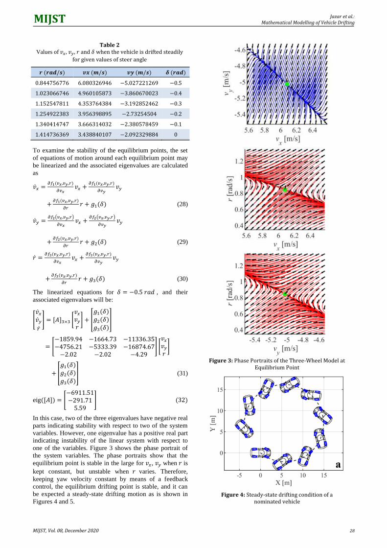
Jazar et al.: Mathematical Modelling of Vehicle Drifting
MIJST, Vol. 08, December 2020 28
Table 2 Values of 𝑣𝑥, 𝑣𝑦, 𝑟 and 𝛿 when the vehicle is drifted steadily
for given values of steer angle
𝒓 (𝒓𝒂𝒅/𝒔) 𝒗𝒙 (𝒎/𝒔) 𝒗𝒚 (𝒎/𝒔) 𝜹 (𝒓𝒂𝒅)
0.844756776 6.080326946 −5.027221269 −0.5
1.023066746 4.960105873 −3.860670023 −0.4
1.152547811 4.353764384 −3.192852462 −0.3
1.254922383 3.956398895 −2.73254504 −0.2
1.340414747 3.666314032 −2.380578459 −0.1
1.414736369 3.438840107 −2.092329884 0
To examine the stability of the equilibrium points, the set
of equations of motion around each equilibrium point may
be linearized and the associated eigenvalues are calculated
as
��𝑥 =𝜕𝑓1(𝑣𝑥,𝑣𝑦,𝑟)
𝜕𝑣𝑥𝑣𝑥 +
𝜕𝑓1(𝑣𝑥,𝑣𝑦,𝑟)
𝜕𝑣𝑦𝑣𝑦
+𝜕𝑓1(𝑣𝑥,𝑣𝑦,𝑟)
𝜕𝑟𝑟 + 𝑔1(𝛿) (28)
��𝑦 =𝜕𝑓2(𝑣𝑥,𝑣𝑦,𝑟)
𝜕𝑣𝑥𝑣𝑥 +
𝜕𝑓2(𝑣𝑥,𝑣𝑦,𝑟)
𝜕𝑣𝑦𝑣𝑦
+𝜕𝑓2(𝑣𝑥,𝑣𝑦,𝑟)
𝜕𝑟𝑟 + 𝑔2(𝛿) (29)
�� =𝜕𝑓3(𝑣𝑥,𝑣𝑦,𝑟)
𝜕𝑣𝑥𝑣𝑥 +
𝜕𝑓3(𝑣𝑥,𝑣𝑦,𝑟)
𝜕𝑣𝑦𝑣𝑦
+𝜕𝑓3(𝑣𝑥,𝑣𝑦,𝑟)
𝜕𝑟𝑟 + 𝑔3(𝛿) (30)
The linearized equations for 𝛿 = −0.5 𝑟𝑎𝑑 , and their
associated eigenvalues will be:
[��𝑥
��𝑦
��
] = [𝐴]3×3 [𝑣𝑥
𝑣𝑦
𝑟] + [
𝑔1(𝛿)𝑔2(𝛿)
𝑔3(𝛿)]
= [−1859.94 −1664.73 −11336.35−4756.21 −5333.39 −16874.67
−2.02 −2.02 −4.29] [
𝑣𝑥
𝑣𝑦
𝑟]
+ [
𝑔1(𝛿)𝑔2(𝛿)
𝑔3(𝛿)] (31)
eig([𝐴]) = [−6911.51−291.71
5.59] (32)
In this case, two of the three eigenvalues have negative real
parts indicating stability with respect to two of the system
variables. However, one eigenvalue has a positive real part
indicating instability of the linear system with respect to
one of the variables. Figure 3 shows the phase portrait of
the system variables. The phase portraits show that the
equilibrium point is stable in the large for 𝑣𝑥, 𝑣𝑦 when 𝑟 is
kept constant, but unstable when 𝑟 varies. Therefore,
keeping yaw velocity constant by means of a feedback
control, the equilibrium drifting point is stable, and it can
be expected a steady-state drifting motion as is shown in
Figures 4 and 5.
Figure 3: Phase Portraits of the Three-Wheel Model at
Equilibrium Point
Figure 4: Steady-state drifting condition of a nominated vehicle

Jazar et al.: Mathematical Modelling of Vehicle Drifting
MIJST, Vol. 08, December 2020 29
Figure 5: Nominated vehicle’s path in the global coordinate frame
5. CONCLUSIONS
This paper introduces a condition for steady-state drifting
condition of the vehicle by investigating equilibrium points
of the equations of motion of vehicles. The lateral and
longitudinal load transfer has been included. The tyre
model also was capable to consider the combined slips as
well as combined saturation of tyre forces. The equations
of motion at steady state condition have been reduced to a
set of nonlinear coupled algebraic equations with
longitudinal and lateral velocities, and yaw rate as
unknown. The equations may be loaded by parameters of
any given vehicle to be solved for the unknowns at a given
steer angle input. If there is any solution for the variables,
then they will indicate equilibrium points of drifting. The
stability analysis by employing the eigenvalue method of
the linearized equations around the equilibrium point
determines the stability of the equilibrium point. A sample
example for a set of nominated numerical values as a fixed
steer angle indicated the existence of an equilibrium point
suggesting the existence of steady-state drifting. Stability
analysis of the equilibrium point suggest that it is possible
to keep the vehicle at a steady-state drifting condition
when keeping the value of the yaw rate constant by means
of a control system.
ACKNOWLEDGEMENTS
Authors would like to express their gratitude to the School
of Engineering, RMIT University, Melbourne, Australia.
They also would like to present their appreciation to the
Editors and anonymous reviewers of MIJST for the
insightful inputs to improve the manuscript.
REFERENCES
Abdulrahim, M. (2006). On the dynamics of automobile drifting.
Technical Paper 2006-01-1019, SAE 2006 World Congress
& Exhibition, https://doi.org/10.4271/2006-01-1019
Bobier-Tiu, C. G., Beal, C. E., Kegelman, J. C., Hindiyeh, R. Y.,
& Gerdes, J. C. (2019). Vehicle control synthesis using
phase portraits of planar dynamics, Vehicle System
Dynamics, 57(9), 1318-1337
Edelmann, J., & Plöchl, M. (2009). Handling characteristics and
stability of the steady-state powerslide motion of an
automobile. Regular and Chaotic Dynamics, 14(6), 682,
https://doi.org/10.1134/S1560354709060069
Hindiyeh, R. Y., & Gerdes, J. C. (2009). Equilibrium analysis of
drifting vehicles for control design. ASME 2009 Dynamic
Systems and Control Conference. DSCC2009-2626: 181-
188, https://doi.org/10.1115/DSCC2009-2626
Hindiyeh, R. Y., & Gerdes, J. C. (2014). A controller framework
for autonomous drifting: Design, stability, and experimental
validation. Journal of Dynamic Systems, Measurement, and
Control, 136(5), DS-12-1023: 051015.
https://doi.org/10.1115/1.4027471
Jazar, R. N. (2019). Advanced vehicle dynamics, Springer, New
York
Milani, S., Marzbani, H., & Jazar, R. N. (2019). Vehicle Drifting:
Mathematical Theory and Dynamic Analysis, 5th Recent
Advances in Automotive Engineering (ReCAR 2019),
Mechanical Engineering Multi-Conference 2019, Universiti
Kebangsaan Malaysia, Selangor, 20-22 August 2019
Shi, S., Li, L., Wang, X., Liu, H., Wang, Y. (2017). Analysis of
the vehicle driving stability region based on the bifurcation
of the driving torque and the steering angle. Proc. Inst.
Mech. Eng. Part D J. Automob. Eng. 231, 984–998
Tavernini, D., Massaro, M., Velenis, E., Katzourakis, D. I., &
Lot, R. (2013). Minimum time cornering: the effect of road
surface and car transmission layout. Vehicle System
Dynamics, 51(10), 1533-1547
Velenis, E., Frazzoli, E., & Tsiotras, P. (2010). Steady-state
cornering equilibria and stabilisation for a vehicle during
extreme operating conditions. International Journal of
Vehicle Autonomous Systems, 8 (2-4), 217-241
Velenis, E., Katzourakis, D., Frazzoli, E., Tsiotras, P., & Happee,
R. (2011). Steady-state drifting stabilization of RWD
vehicles. Control Engineering Practice, 19(11), 1363-1376
Voser, C., Hindiyeh, R. Y., & Gerdes, J. C. (2010). Analysis and
control of high sideslip manoeuvres. Vehicle System
Dynamics, 48(S1), 317-336


MIJST MIST International Journal of Science and Technology
MIJST, Vol. 08, December 2020 | https://doi.org/10.47981/j.mijst.08(02)2020.214(31-40) 31
Modeling and Control Simulation of a Robotic Chair-Arm: Protection against COVID-19 in Rehabilitation Exercise
M. Akhtaruzzaman1*, Amir A. Shafie2, Md Raisuddin Khan3, and Md Mozasser Rahman4
1 Dept. of Computer Science and Engineering, Military Institute of Science and Technology (MIST), Dhaka, Bangladesh 2,3 Dept. of Mechatronics Engineering, International Islamic University Malaysia (IIUM), 53100 Kuala Lumpur, Malaysia 4 Dept. of Mechanical Engineering Technology, Universiti Tun Hussein Onn Malaysia (UTHM), 84600 Pagoh, Johor, Malaysia 1 R&D (Robotics) Section, DREAM Robotics Ltd., Dhaka, Bangladesh
emails: *[email protected]; [email protected]; [email protected]; and [email protected]
A R T I C L E I N F O
A B S T R A C T
Article History: Received: 18th July 2020 Revised: 10th September 2020 Accepted: 11th October 2020 Published: 16th December 2020
In the field of rehabilitation, lower-limbs therapeutic exercise has become a challenging job for medical professionals in COVID-19 pandemic. Providing manual therapy to lower limbs is not an easy task and, in most cases, it involves multiple persons. Moreover, it is a monotonous job, and the service providers need to be in close contact with the patient thereby creating the risk of infection. In this circumstance, robot-assisted rehabilitation exercise for lower limbs offers a risk-free solution. This paper presents dynamic modeling and control simulation of One Degree of Freedom robotic chair-arm (robotic arm attached with a special chair). The control structure is designed with two compensators for position and velocity control. The simulation results show that the proposed system has a good potential in providing automatic rehabilitation therapy for lower limbs, especially for knee joint range of motion exercise. The results also indicate faster responses with settling time less than 0.04 second and steady-state error below 0.05. The findings show that a robotic chair arm can be used for providing automatic therapy to patients in situations like COVID-19 pandemic.
Keywords: 1-DoF robotic arm Robotic chair-arm Robot-assisted rehabilitation Lower-limbs therapeutic exercise Robot-assisted system
COVID-19
© 2020 MIJST. All rights reserved.
1. INTRODUCTION
The COVID-19 has become an epidemic throughout the
world which has been forcing humanity to be demobilized
by creating intangible obstacles and threats to fulfill our
five basic needs, foods, clothing, shelter, healthcare, and
education. Healthcare and education sectors are
dangerously affected by the invasion of Corona Virus.
COVID-19 is highly contagious which makes medical
services difficult to provide. Clinical care service is one of
the broad areas where robotics can contribute to change the
sector to reach its highest level (Yang et al., 2020; Zeng,
Chen, & Lew, 2020).
Global demand for rehabilitation services is increasing
because of growing non-communicable diseases like stroke
and heart attacks. Moreover, the current situation of the
global pandemic raises greater demand for robot-assisted
rehabilitation systems in minimizing the risk of
contamination both for healthcare service providers and
patients (Zeng, Chen, & Lew, 2020; Kimmig et al., 2020).
To increase Range of Motion (RoM) flexibility of knee
joint and motor neuron dysfunction, continuous passive
RoM exercise is a monotonous and arduous job in terms of
physical labor and time. Repeated manual exercise also
unable to comply with natural motion patterns during the
whole exercise session. Furthermore, transporting the
patient for each session increases time overheads, cost, and
discomfort to the patients. Thus, to decrease the burden,
design and control simulation of a 1-DoF robotic arm for
knee RoM exercise is presented in this manuscript. The
arm is attached with a special chair so that a disabled
patient can be seated on to receive knee joint RoM
therapeutic exercise.
Robot-assisted rehabilitation exercise for functional
adaptation of knee joint RoM widens a great opportunity
for post-stroke patients (Akhtaruzzaman et al., 2019).
Robot-assisted system also could be a great tool to measure
functional improvements of muscles and joint motions
(Huang et al., 2019). The instrumentation system of a
robotic arm can perform precise measurement of positions
and forces and able to co-operate with human (Shi et al.,
2019). More importantly, electro-mechanical actuators of
the system can perform a task repeatedly within the desired
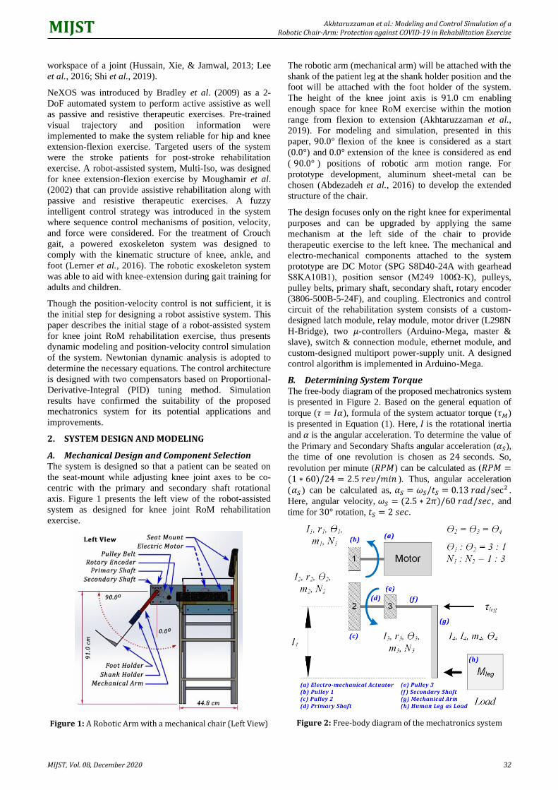
Akhtaruzzaman et al.: Modeling and Control Simulation of a Robotic Chair-Arm: Protection against COVID-19 in Rehabilitation Exercise
MIJST, Vol. 08, December 2020 32
workspace of a joint (Hussain, Xie, & Jamwal, 2013; Lee
et al., 2016; Shi et al., 2019).
NeXOS was introduced by Bradley et al. (2009) as a 2-
DoF automated system to perform active assistive as well
as passive and resistive therapeutic exercises. Pre-trained
visual trajectory and position information were
implemented to make the system reliable for hip and knee
extension-flexion exercise. Targeted users of the system
were the stroke patients for post-stroke rehabilitation
exercise. A robot-assisted system, Multi-Iso, was designed
for knee extension-flexion exercise by Moughamir et al.
(2002) that can provide assistive rehabilitation along with
passive and resistive therapeutic exercises. A fuzzy
intelligent control strategy was introduced in the system
where sequence control mechanisms of position, velocity,
and force were considered. For the treatment of Crouch
gait, a powered exoskeleton system was designed to
comply with the kinematic structure of knee, ankle, and
foot (Lerner et al., 2016). The robotic exoskeleton system
was able to aid with knee-extension during gait training for
adults and children.
Though the position-velocity control is not sufficient, it is
the initial step for designing a robot assistive system. This
paper describes the initial stage of a robot-assisted system
for knee joint RoM rehabilitation exercise, thus presents
dynamic modeling and position-velocity control simulation
of the system. Newtonian dynamic analysis is adopted to
determine the necessary equations. The control architecture
is designed with two compensators based on Proportional-
Derivative-Integral (PID) tuning method. Simulation
results have confirmed the suitability of the proposed
mechatronics system for its potential applications and
improvements.
2. SYSTEM DESIGN AND MODELING
A. Mechanical Design and Component Selection The system is designed so that a patient can be seated on
the seat-mount while adjusting knee joint axes to be co-
centric with the primary and secondary shaft rotational
axis. Figure 1 presents the left view of the robot-assisted
system as designed for knee joint RoM rehabilitation
exercise.
Figure 1: A Robotic Arm with a mechanical chair (Left View)
The robotic arm (mechanical arm) will be attached with the
shank of the patient leg at the shank holder position and the
foot will be attached with the foot holder of the system.
The height of the knee joint axis is 91.0 cm enabling
enough space for knee RoM exercise within the motion
range from flexion to extension (Akhtaruzzaman et al.,
2019). For modeling and simulation, presented in this
paper, 90.0° flexion of the knee is considered as a start
(0.0°) and 0.0° extension of the knee is considered as end
( 90.0° ) positions of robotic arm motion range. For
prototype development, aluminum sheet-metal can be
chosen (Abdezadeh et al., 2016) to develop the extended
structure of the chair.
The design focuses only on the right knee for experimental
purposes and can be upgraded by applying the same
mechanism at the left side of the chair to provide
therapeutic exercise to the left knee. The mechanical and
electro-mechanical components attached to the system
prototype are DC Motor (SPG S8D40-24A with gearhead
S8KA10B1), position sensor (M249 100Ω-K), pulleys,
pulley belts, primary shaft, secondary shaft, rotary encoder
(3806-500B-5-24F), and coupling. Electronics and control
circuit of the rehabilitation system consists of a custom-
designed latch module, relay module, motor driver (L298N
H-Bridge), two 𝜇-controllers (Arduino-Mega, master &
slave), switch & connection module, ethernet module, and
custom-designed multiport power-supply unit. A designed
control algorithm is implemented in Arduino-Mega.
B. Determining System Torque The free-body diagram of the proposed mechatronics system
is presented in Figure 2. Based on the general equation of
torque (𝜏 = 𝐼𝛼), formula of the system actuator torque (𝜏𝑀)
is presented in Equation (1). Here, 𝐼 is the rotational inertia
and 𝛼 is the angular acceleration. To determine the value of
the Primary and Secondary Shafts angular acceleration (𝛼𝑆),
the time of one revolution is chosen as 24 seconds. So,
revolution per minute (𝑅𝑃𝑀) can be calculated as (𝑅𝑃𝑀 =(1 ∗ 60)/24 = 2.5 𝑟𝑒𝑣/𝑚𝑖𝑛 ). Thus, angular acceleration
(𝛼𝑆 ) can be calculated as, 𝛼𝑆 = 𝜔𝑆/𝑡𝑆 = 0.13 𝑟𝑎𝑑/sec2 .
Here, angular velocity, 𝜔𝑆 = (2.5 ∗ 2𝜋)/60 𝑟𝑎𝑑/𝑠𝑒𝑐, and
time for 30° rotation, 𝑡𝑆 = 2 𝑠𝑒𝑐.
Figure 2: Free-body diagram of the mechatronics system

Akhtaruzzaman et al.: Modeling and Control Simulation of a Robotic Chair-Arm: Protection against COVID-19 in Rehabilitation Exercise
MIJST, Vol. 08, December 2020 33
𝜏𝑀 =
1
2𝑚1𝑟1
2𝛼1 +
(𝑁1
𝑁2)2{𝛼𝑆 (
1
2(𝑚2𝑟2
2 +𝑚3𝑟32) +
1
3𝑚4𝑙4
2) + 𝜏𝑙𝑒𝑔} (1)
Here, 𝑚 is mass, 𝑟 is pulley radius, 𝜃 is angular deflection,
𝑁 is pulley teeth, and 𝑙 is the length of the mechanical arm.
By considering the relations, 𝛼1 = 𝛼𝑆(𝑁2/𝑁1) and
(𝑁1/𝑁2) = 𝑁𝑆 , the actuator torque equation can be
modified as shown in Equation (2). Here, 𝑁1: 𝑁2 = 1: 3.
The necessary values of the parameters are presented in
Table 1. Required torques at the knee joint, while the
patient is in a sitting position, are identified from the study
conducted by Akhtaruzzaman et al. (2019).
𝜏𝑀 =
𝛼𝑆2{1
𝑁𝑆(𝑚1𝑟1
2)+𝑁𝑆2 (𝑚2𝑟2
2 +𝑚3𝑟32 +
2
3𝑚4𝑙4
2)}
+𝑁𝑆2𝜏𝑙𝑒𝑔
(2)
Table 1 Parameters to Calculate Required Torque of the
System Actuator
Parameter Symbols Values
𝑚1 030.0 𝑔
𝑚2 751.0 𝑔
𝑚3 215.0 𝑔
𝑚4 350.0 𝑔
𝑟1 01.50 𝑐𝑚
𝑟2 04.50 𝑐𝑚
𝑟3 03.25 𝑐𝑚
𝑙4 30.00 𝑐𝑚
𝛼𝑆 0.1300 ∗ (180 π⁄ ) 𝑑𝑒𝑔
𝑠𝑒𝑐2 ⁄
𝑁1 20.0 teeth
𝑁2 60.0 teeth
𝜏𝑙𝑒𝑔 {895.1 𝑁. 𝑐𝑚 𝑓𝑜𝑟 𝜃1 = 0°300.0 𝑁. 𝑐𝑚 𝑓𝑜𝑟 𝜃1 = 65°
Required torque of the system actuator is calculated as
100.4 𝑁. 𝑐𝑚 for knee joint torque as 895.1 𝑁. 𝑐𝑚 at full
extension of the knee. For the 25° position of knee joint
(knee joint torque is 300.0 𝑁. 𝑐𝑚), the required torque of
the system actuator is determined as 034.3 𝑁. 𝑐𝑚 . By
considering the safety factor as 𝑆𝑓 = 1.5, calculated required
torques are presented in Equation (3).
𝜏𝑚 = {(𝜏𝑀 × 𝑠𝑓) ≈ 150.0 𝑁. 𝑐𝑚 𝑓𝑜𝑟 𝜃1 = 90°
(𝜏𝑀 × 𝑠𝑓) ≈ 050.0 𝑁. 𝑐𝑚 𝑓𝑜𝑟 𝜃1 = 25° (3)
C. System Dynamics The conceptual Electro-mechanical model of the system
actuator is presented in Figure 3. Here 𝜏𝑚 is rotor torque
produced by the applied current (𝑖(𝑡)) from 𝑉 DC source.
The 𝜏𝑚 is proportional to its magnitude. Effective inertia of
armature is presented by 𝐼𝑚 . Angular deflection (𝜃(𝑡)) of
the rotor produces back Electromotive Force (EMF) (𝐸𝑏(𝑡)) which is proportional to rotor angular velocity (𝑑𝜃(𝑡)/
𝑑(𝑡) = ��(𝑡)). Input-output ratio of gearhead is presented as,
(𝑁𝑚: 𝑁𝐿 = 1: 10). The friction force of the gearhead module
is zero (𝜏𝑓𝑚 = 0). The actuator module is connected with a
switching module which is controlled by the control signals
through Pulse Width Modulation (PWM) module.
Figure 3: Conceptual Electro-mechanical model of DC Motor
Based on the characteristics of this electro-mechanical
module, two differential equations can be presented as
shown in Equation (4). In the equation, the constant
parameters are, coil resistance (𝑅𝑚 ), inductance ( 𝐿𝑚 ),
torque constant (𝐾𝜏𝑚 ), and back EMF (𝐾𝑏𝑚 ). Armature
inertia, viscous friction, armature load, and external load are
presented by 𝐼𝑚, 𝐵𝑚, 𝜏𝑚 and 𝜏𝐿, respectively.
𝐿𝑚𝑑𝑖(𝑡)
𝑑𝑡+ 𝐾𝑏𝑚
𝑑𝜃𝑚(𝑡)
𝑑𝑡+ 𝑅𝑚𝑖(𝑡) − 𝑣𝑚(𝑡) = 0
𝐼𝑚𝑑2𝜃𝑚(𝑡)
𝑑𝑡2+ 𝐵𝑚
𝑑𝜃𝑚(𝑡)
𝑑𝑡+
𝑁𝑚
𝑁𝐿(𝜏𝐿) − 𝐾𝜏𝑚𝑖(𝑡) = 0
} ()
Now, from the free-body diagram in Figure 2, the external
load (𝜏𝐿) can be formulated, as shown in Equation (5).
𝜏𝐿 = (𝐼1 + (𝑁1
𝑁2)2
(𝐼2 + 𝐼3 + 𝐼4 + 𝐼𝑙𝑒𝑔))𝑑2𝜃1(𝑡)
𝑑𝑡2 ()
Now by replacing 𝜏𝐿 in the second part of Equation (4),
Equation (6) can be formulated which is the necessary
differential equation of the proposed system. Here, 𝜃𝐿 = 𝜃1,
𝑁𝐿 = 𝑁1 , and 𝑁𝑚
𝑁𝐿⁄ =
𝜃1𝜃𝑚⁄ are applied to establish a
relation with control parameter 𝜃1 . Necessary parameter
definitions are presented in Equation (7). Table 2 presents
the necessary parameter values of the system dynamic
model.
𝐿𝑚𝑑𝑖(𝑡)
𝑑𝑡+ 𝐾𝑏𝑚𝑁𝑅𝑚
𝑑𝜃1(𝑡)
𝑑𝑡+ 𝑅𝑚𝑖(𝑡) − 𝑣𝑚(𝑡) = 0
𝐼𝐸𝑄𝑑2𝜃1(𝑡)
𝑑𝑡2+ 𝐵𝐸𝑄
𝑑𝜃1(𝑡)
𝑑𝑡− 𝐾𝜏𝑚𝑖(𝑡) = 0
} ()
𝐼𝐸𝑄 = 𝑁𝑅𝑚𝐼𝑚 +1
𝑁𝑅𝑚(𝐼1 + 𝑁𝑅
2(𝐼2 + 𝐼3 + 𝐼4 + 𝐼𝑙𝑒𝑔))
𝐵𝐸𝑄= 𝑁𝑅𝑚𝐵𝑚
𝑁𝑅 =𝑁1
𝑁2
𝑁𝑅𝑚=𝑁𝐿
𝑁𝑚
𝐼1 =1
2𝑚1𝑟1
2
𝐼2 =1
2𝑚2𝑟2
2
𝐼3 =1
2𝑚3𝑟3
2
𝐼4 =1
3𝑚4𝑙4
2
𝐼𝑙𝑒𝑔 = 𝑚𝑙𝑒𝑔𝑙𝑐𝑜𝑚𝑙𝑒𝑔
2}
()
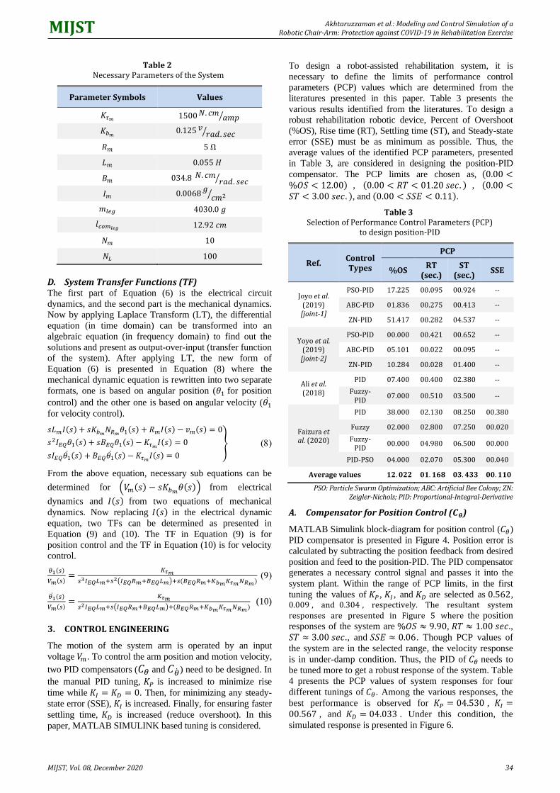
Akhtaruzzaman et al.: Modeling and Control Simulation of a Robotic Chair-Arm: Protection against COVID-19 in Rehabilitation Exercise
MIJST, Vol. 08, December 2020 34
Table 2 Necessary Parameters of the System
Parameter Symbols Values
𝐾𝜏𝑚 1500𝑁. 𝑐𝑚 𝑎𝑚𝑝⁄
𝐾𝑏𝑚 0.125𝑣 𝑟𝑎𝑑. 𝑠𝑒𝑐⁄
𝑅𝑚 5 Ω
𝐿𝑚 0.055 𝐻
𝐵𝑚 034.8 𝑁. 𝑐𝑚 𝑟𝑎𝑑. 𝑠𝑒𝑐⁄
𝐼𝑚 0.0068𝑔𝑐𝑚2⁄
𝑚𝑙𝑒𝑔 4030.0 𝑔
𝑙𝑐𝑜𝑚𝑙𝑒𝑔 12.92 𝑐𝑚
𝑁𝑚 10
𝑁𝐿 100
D. System Transfer Functions (TF) The first part of Equation (6) is the electrical circuit
dynamics, and the second part is the mechanical dynamics.
Now by applying Laplace Transform (LT), the differential
equation (in time domain) can be transformed into an
algebraic equation (in frequency domain) to find out the
solutions and present as output-over-input (transfer function
of the system). After applying LT, the new form of
Equation (6) is presented in Equation (8) where the
mechanical dynamic equation is rewritten into two separate
formats, one is based on angular position (𝜃1 for position
control) and the other one is based on angular velocity (𝜃1
for velocity control).
𝑠𝐿𝑚𝐼(𝑠) + 𝑠𝐾𝑏𝑚𝑁𝑅𝑚𝜃1(𝑠) + 𝑅𝑚𝐼(𝑠) − 𝑣𝑚(𝑠) = 0
𝑠2𝐼𝐸𝑄𝜃1(𝑠) + 𝑠𝐵𝐸𝑄𝜃1(𝑠) − 𝐾𝜏𝑚𝐼(𝑠) = 0
𝑠𝐼𝐸𝑄𝜃1(𝑠) + 𝐵𝐸𝑄𝜃1(𝑠) − 𝐾𝜏𝑚𝐼(𝑠) = 0
} ()
From the above equation, necessary sub equations can be
determined for (𝑉𝑚(𝑠) − 𝑠𝐾𝑏𝑚𝜃(𝑠)) from electrical
dynamics and 𝐼(𝑠) from two equations of mechanical
dynamics. Now replacing 𝐼(𝑠) in the electrical dynamic
equation, two TFs can be determined as presented in
Equation (9) and (10). The TF in Equation (9) is for
position control and the TF in Equation (10) is for velocity
control.
𝜃1(𝑠)
𝑉𝑚(𝑠)=
𝐾𝜏𝑚
𝑠3𝐼𝐸𝑄𝐿𝑚+𝑠2(𝐼𝐸𝑄𝑅𝑚+𝐵𝐸𝑄𝐿𝑚)+𝑠(𝐵𝐸𝑄𝑅𝑚+𝐾𝑏𝑚𝐾𝜏𝑚𝑁𝑅𝑚)
()
𝜃1(𝑠)
𝑉𝑚(𝑠)=
𝐾𝜏𝑚
𝑠2𝐼𝐸𝑄𝐿𝑚+𝑠(𝐼𝐸𝑄𝑅𝑚+𝐵𝐸𝑄𝐿𝑚)+(𝐵𝐸𝑄𝑅𝑚+𝐾𝑏𝑚𝐾𝜏𝑚𝑁𝑅𝑚) (10)
3. CONTROL ENGINEERING
The motion of the system arm is operated by an input
voltage 𝑉𝑚. To control the arm position and motion velocity,
two PID compensators (𝐶𝜃 and 𝐶��) need to be designed. In
the manual PID tuning, 𝐾𝑃 is increased to minimize rise
time while 𝐾𝐼 = 𝐾𝐷 = 0. Then, for minimizing any steady-
state error (SSE), 𝐾𝐼 is increased. Finally, for ensuring faster
settling time, 𝐾𝐷 is increased (reduce overshoot). In this
paper, MATLAB SIMULINK based tuning is considered.
To design a robot-assisted rehabilitation system, it is
necessary to define the limits of performance control
parameters (PCP) values which are determined from the
literatures presented in this paper. Table 3 presents the
various results identified from the literatures. To design a
robust rehabilitation robotic device, Percent of Overshoot
(%OS), Rise time (RT), Settling time (ST), and Steady-state
error (SSE) must be as minimum as possible. Thus, the
average values of the identified PCP parameters, presented
in Table 3, are considered in designing the position-PID
compensator. The PCP limits are chosen as, (0.00 <%𝑂𝑆 < 12.00) , (0.00 < 𝑅𝑇 < 01.20 𝑠𝑒𝑐. ) , (0.00 <𝑆𝑇 < 3.00 𝑠𝑒𝑐. ), and (0.00 < 𝑆𝑆𝐸 < 0.11).
Table 3 Selection of Performance Control Parameters (PCP)
to design position-PID
Ref. Control Types
PCP
%OS RT
(sec.) ST
(sec.) SSE
Joyo et al. (2019)
[joint-1]
PSO-PID 17.225 00.095 00.924 --
ABC-PID 01.836 00.275 00.413 --
ZN-PID 51.417 00.282 04.537 --
Yoyo et al. (2019)
[joint-2]
PSO-PID 00.000 00.421 00.652 --
ABC-PID 05.101 00.022 00.095 --
ZN-PID 10.284 00.028 01.400 --
Ali et al. (2018)
PID 07.400 00.400 02.380 --
Fuzzy-PID
07.000 00.510 03.500 --
Faizura et al. (2020)
PID 38.000 02.130 08.250 00.380
Fuzzy 02.000 02.800 07.250 00.020
Fuzzy-PID
00.000 04.980 06.500 00.000
PID-PSO 04.000 02.070 05.300 00.040
Average values 𝟏𝟐. 𝟎𝟐𝟐 𝟎𝟏. 𝟏𝟔𝟖 𝟎𝟑. 𝟒𝟑𝟑 𝟎𝟎. 𝟏𝟏𝟎
PSO: Particle Swarm Optimization; ABC: Artificial Bee Colony; ZN: Zeigler-Nichols; PID: Proportional-Integral-Derivative
A. Compensator for Position Control (𝑪𝜽)
MATLAB Simulink block-diagram for position control (𝐶𝜃)
PID compensator is presented in Figure 4. Position error is
calculated by subtracting the position feedback from desired
position and feed to the position-PID. The PID compensator
generates a necessary control signal and passes it into the
system plant. Within the range of PCP limits, in the first
tuning the values of 𝐾𝑃 , 𝐾𝐼 , and 𝐾𝐷 are selected as 0.562, 0.009 , and 0.304 , respectively. The resultant system
responses are presented in Figure 5 where the position
responses of the system are %𝑂𝑆 ≈ 9.90, 𝑅𝑇 ≈ 1.00 𝑠𝑒𝑐., 𝑆𝑇 ≈ 3.00 𝑠𝑒𝑐., and 𝑆𝑆𝐸 ≈ 0.06. Though PCP values of
the system are in the selected range, the velocity response
is in under-damp condition. Thus, the PID of 𝐶𝜃 needs to
be tuned more to get a robust response of the system. Table
4 presents the PCP values of system responses for four
different tunings of 𝐶𝜃. Among the various responses, the
best performance is observed for 𝐾𝑃 = 04.530 , 𝐾𝐼 =00.567 , and 𝐾𝐷 = 04.033 . Under this condition, the
simulated response is presented in Figure 6.

Akhtaruzzaman et al.: Modeling and Control Simulation of a Robotic Chair-Arm: Protection against COVID-19 in Rehabilitation Exercise
MIJST, Vol. 08, December 2020 35
Figure 4: Control architecture (MATLAB Simulink diagram) in designing 𝐶𝜃 PID Compensator
Figure 5: System response for PID compensator 𝐶𝜃 where 𝐾𝑃 = 0.562, 𝐾𝐼 = 0.009, and 𝐾𝐷 = 0.304
According to the graph (Figure 6), no overshoot is
observed for the position response (%𝑂𝑆 = 00.00), the
steady-state error is observed as a minimum ( 𝐸𝑆𝑆 =0.050). The system also shows the faster rise time and
faster settling time ( 𝑅𝑇 = 00.240 𝑠𝑒𝑐. and 𝑆𝑇 =00.300 𝑠𝑒𝑐.).
Table 4
Various PCP values for different tuning of position-PID (𝐶𝜃)
Tu
ne
PID Values
PCP
%OS RT
(sec.) ST
(sec.) SSE
1st 𝐾𝑃 = 00.562 𝐾𝐼 = 00.009 𝐾𝐷 = 00.304
09.900 01.000 03.000 00.060
2nd 𝐾𝑃 = 01.099 𝐾𝐼 = 00.049 𝐾𝐷 = 01.109
00.000 00.859 01.040 00.080
3rd 𝑲𝑷 = 𝟎𝟒. 𝟓𝟑𝟎 𝑲𝑰 = 𝟎𝟎. 𝟓𝟔𝟕 𝑲𝑫 = 𝟎𝟒. 𝟎𝟑𝟑
𝟎𝟎. 𝟎𝟎𝟎 𝟎𝟎. 𝟐𝟒𝟎 𝟎𝟎. 𝟑𝟎𝟎 𝟎𝟎. 𝟎𝟓𝟎
4th 𝐾𝑃 = 52.979 𝐾𝐼 = 29.090 𝐾𝐷 = 21.437
01.300 00.054 0.277 00.060
Figure 6: System response (3rd tuning) for PID compensator 𝐶𝜃 where 𝐾𝑃 = 4.530, 𝐾𝐼 = 0.567, and 𝐾𝐷 = 4.033
B. Compensator for Velocity Control (𝑪��)
A robot-assisted rehabilitation system must have the
capability to follow a trajectory with the desired velocity.
The sudden change of velocity may cause the system to
unstable creating secondary injury to the targeted limbs. In
Figure 6, the velocity response shows high deflection, thus it
is necessary to design 2nd compensator (𝐶��) for velocity
control. The control architecture is presented in Figure 7.
Considering the chosen PCP limits, the values of 𝐾𝑃, 𝐾𝐼 , and
𝐾𝐷 are tuned as 140.00, 18416.00, and 00.10, respectively.
Table 5 presents the various responses of four different trials
from where the results of the 3rd trial are considered, thus
selected the velocity-PID parameter values. To design the
control architecture, the switching mechanism is adopted.
The philosophy behind this technique is that the velocity-
PID will dominate to maintain the desired constant
velocity during motion and the control responsibility will
switch to the position-PID at the moment of the system
arm reaches the desired position and maintain the desired
angular state.

Akhtaruzzaman et al.: Modeling and Control Simulation of a Robotic Chair-Arm: Protection against COVID-19 in Rehabilitation Exercise
MIJST, Vol. 08, December 2020 36
Table 5
Various PCP values for different tuning of velocity-PID (𝐶��)
Tu
ne
PID Values
PCP
%OS RT
(sec.) ST
(sec.) SSE
1st 𝐾𝑃 = 45.00 𝐾𝐼 = 8516.00 𝐾𝐷 = 00.80
25.600 00.021 00.356 −0.120
2nd 𝐾𝑃 = 80.00
𝐾𝐼 = 18516.00 𝐾𝐷 = 00.20
34.700 00.009 00.069 −0.018
3rd 𝑲𝑷 = 𝟏𝟒𝟎. 𝟎𝟎 𝑲𝑰 = 𝟏𝟖𝟒𝟏𝟔. 𝟎𝟎 𝑲𝑫 = 𝟎𝟎. 𝟏𝟎
𝟐𝟗. 𝟓𝟎𝟎 𝟎𝟎. 𝟎𝟎𝟔 𝟎𝟎. 𝟎𝟐𝟖 −𝟎.𝟎𝟏𝟗
4th 𝐾𝑃 = 180.00 𝐾𝐼 = 29323.00 𝐾𝐷 = 00.10
41.500 Unstable
The system plant (system dynamic model) is basically a
Single-Input Multi-Output (SIMO) system as both position
and velocity outputs depend on the input of electric voltage
( 𝑉𝑚 ) to the system plant. The design of the control
architecture reflects the parallel configuration of two
compensators. Here the position and velocity errors are
feed to position-PID ( 𝐶𝜃 ) and velocity-PID ( 𝐶�� )
compensators separately. The output of both PIDs is then
summed up and feed as a single input to the system plant.
To observe the system performance, the designed
architecture is simulated for a constant velocity input as
10 𝑑𝑒𝑔./𝑠𝑒𝑐. while a step input is applied for position
change from 0.0° to 20.00° . At this condition, the arm
must rise to its desired angle within two seconds while
maintaining the desired velocity complying with the
selected PCP characteristics. Figure 8 shows the simulated
responses of the system and corresponding error
characteristics for such input conditions.
Figure 7: Control architecture (MATLAB Simulink diagram) in designing 𝐶𝜃 and 𝐶�� PID Compensators
Figure 8: System responses (3rd tuning) of velocity-PID (𝐶��)
4. RESULTS AND DISCUSSION
Results of the designed architecture show a stable system
response both in position and velocity control. The desired
position and velocity of the robot arm are achieved within
the desired PCP value ranges. The system is simulated for
various input conditions to confirm the suitability of the
designed control architecture. Figure 8 has presented the
simulated results of the system for the input parameters as
0.0° to 20.0° motion range with a constant velocity of
10.0 𝑑𝑒𝑔./𝑠𝑒𝑐. Angle rise time satisfies the desired time
for about two seconds with a smooth motion trajectory.
Though some deflections are observed for velocity
response at the initiation and termination of motion, the
results of position control satisfy selected PCP ranges.
Figure 9 presents clear observations of velocity response
and the corresponding error characteristics at the initiation
of motion. The graph shows that the rise time is about
0.006 𝑠𝑒𝑐. with the percent of overshoot is about 29.50.
The settling time of the velocity response is around
0.028 𝑠𝑒𝑐. and steady-state error is almost 0.019 . The
results comply with the PCP value ranges for position

Akhtaruzzaman et al.: Modeling and Control Simulation of a Robotic Chair-Arm: Protection against COVID-19 in Rehabilitation Exercise
MIJST, Vol. 08, December 2020 37
response, thus ensure the suitability of the designed control
architecture.
Figure 9: Velocity response and corresponding errors of the system at the initiation of motion
Motion termination occurs when the system reaches the
desired angular position. At this moment, the switching is
activated, and the control is switched back to the position-
PID compensator to hold the arm at the desired angle. At
the same time, the velocity reaches zero. Figure 10 shows
the velocity response of the system at the termination of
motion. The graph shows that the rise time is around
0.006 𝑠𝑒𝑐., settling time is about 0.027 𝑠𝑒𝑐., and steady-
state error is 0.0037. The percent of overshoot is detected
as 16.20 . For a rising motion of the system arm, two
switching conditions have occurred, one is position-PID to
velocity-PID at the initiation of motion (hold at 0.0° to
swing) and the other is velocity-PID to position-PID at the
termination of motion (swing to hold at 20.0° ). A
comparison of the velocity responses in between these two
switching conditions reflects that all the PCP values at
motion-termination are lower than motion-initiation. This
behavior explains that the system needs less energy to
settle down the velocity to zero at hold condition.
Opposingly, the system needs high energy at the motion-
initiation state to maintain the desired velocity. A similar
test with different input conditions is simulated resulting in
the same behavior of the system response. The system is
also tested with an external disturbance input. The
disturbance is applied at the position response of the
system to observe the effects on system stability in terms
of position and velocity responses. Figure 11 shows the
system control architecture with an Impulse Generator (IG)
as an external disturbance to the position output (𝜃) of the
plant.
Figure 10: Velocity response and corresponding errors of the system at the termination of motion
Figure 11: System control architecture with an external disturbance at the position output just before the position feedback

Akhtaruzzaman et al.: Modeling and Control Simulation of a Robotic Chair-Arm: Protection against COVID-19 in Rehabilitation Exercise
MIJST, Vol. 08, December 2020 38
The IG generates a single pulse of 0.001 𝑠𝑒𝑐. pulse width
and 10.00° amplitude. The impulse signal is added with
the 𝜃output response of the system; thus, position response
reflects a sharp rise and falls at a specific time of the
system operation. For the test simulation, two impulse
signals are applied, i) a positive impulse during motion at
4.70 𝑠𝑒𝑐., and ii) a negative impulse during 45.00°hold
condition at 6.00 𝑠𝑒𝑐. Figure 12 shows the system
response for the input parameters as 10.00 𝑑𝑒𝑔./𝑠𝑒𝑐. velocity and step function from 0.0° to 45.00°.
Figure 12: System position and velocity responses for Position set-point at 45.0° and Velocity set-point at
10.0 𝑑𝑒𝑔./𝑠𝑒𝑐. while external disturbances are at 4.70 𝑠𝑒𝑐. (positive disturbance) and at 6.00 𝑠𝑒𝑐. (negative disturbance)
According to the above figure, the position response of the
system shows a smooth transition at the initiation and
termination of motion. Velocity response shows some
deflections at the initiation at time 1.00 𝑠𝑒𝑐. and
termination of the motion at 5.50 𝑠𝑒𝑐. The behavior is
clearly presented in Figure 13 where (a) reflects velocity
response with error behavior at the initiation and (b) shows
velocity response with corresponding error behavior at the
termination of motion. From the response graphs, the PCP
values are extracted as %𝑂𝑆 = 47.30 , 𝑅𝑇 = 0.006 𝑠𝑒𝑐. , 𝑆𝑇 = 0.033 𝑠𝑒𝑐. and 𝑆𝑆𝐸 = −0.044 at the initiation of
motion and %𝑂𝑆 = 15.34 ., 𝑅𝑇 = 0.006 𝑠𝑒𝑐. , 𝑆𝑇 =0.031 𝑠𝑒𝑐. , and 𝑆𝑆𝐸 = 0.0041 at the termination of
motion. The response of the system for positive impulse
disturbance at 4.70 𝑠𝑒𝑐. during motion and negative
impulse disturbance at 6.00 𝑠𝑒𝑐. during the 45.00° hold
position are presented in Figure 14 and Figure 15,
respectively. For the positive impulse during rising motion,
velocity goes down to about 9.713 𝑑𝑒𝑔./𝑠𝑒𝑐. and reaches
to the desired velocity (≈ 10.00 𝑑𝑒𝑔./𝑠𝑒𝑐.) at 4.728 𝑠𝑒𝑐., reflecting 𝑆𝑇 = 0.028 𝑠𝑒𝑐. , %𝑂𝑆 = 2.787 , 𝑅𝑇 =0.008 𝑠𝑒𝑐. and 𝑆𝑆𝐸 = 0.0030. For the negative impulse,
the desired velocity rises to its set point and falls to zero
reflecting the impulse disturbance to the velocity input
(Figure 15). Velocity response rises to 4.603 𝑑𝑒𝑔./𝑠𝑒𝑐. and settles down to zero by 0.022 𝑠𝑒𝑐. with %𝑂𝑆 = 5.110,
as presented in Figure 15.
Figure 13: Velocity responses and error behaviors; (a) at motion initiation, and (b) at motion termination
Figure 14: Velocity responses of the system for positive disturbance (position) input at 4.7 𝑠𝑒𝑐.
Figure 15: Velocity responses for negative disturbance (position) at 6.00 𝑠𝑒𝑐. while robot-arm is holding at 45°

Akhtaruzzaman et al.: Modeling and Control Simulation of a Robotic Chair-Arm: Protection against COVID-19 in Rehabilitation Exercise
MIJST, Vol. 08, December 2020 39
For the impulse disturbance, system output shows a very
little impact on the position ( 𝜃 ) response. Figure 16
presents the position response for −10° impulse at
6.00 𝑠𝑒𝑐. while the robot arm is in holding a position at
45.00° angles. From various simulation results, it is
observed that the system shows good performances while
the velocity range is 0.00 < �� < 14.00 𝑑𝑒𝑔./𝑠𝑒𝑐. At
0.00 𝑑𝑒𝑔./𝑠𝑒𝑐. there is no angular motion observed at the
robot arm. Conversely, the velocity greater than
14.00 𝑑𝑒𝑔./𝑠𝑒𝑐. makes the system unstable. Table 6
presents the PCP values of position and velocity responses
for various input conditions.
Figure 16: Position (𝜃) response of the system for −10° impulse disturbance at 6.00 𝑠𝑒𝑐. while the robot arm is
holding at 45.0° angle
Table 6 System PCP values of position and velocity
responses for various input conditions
Input Conditions
Outputs
PCP Values
%OS RT
(sec.) ST
(sec.) SSE
Ste
p: 𝟎° 𝒕𝒐 𝟐𝟎°
𝜽: 𝟏𝟎 𝒅𝒆𝒈.𝒔𝒆𝒄
⁄.
�� @ start of motion
29.50 0.006 0.028 0.0190
�� @ end of motion
16.20 0.006 0.027 0.0037
�� for +10° impulse @
motion 19.66 0.009 0.031 0.0030
�� for +10° impulse @ 20° hold
5.405 0.010 0.022 0.0030
𝜃 for +10° impulse @ 20° hold
0.036 0.007 0.025 0.0016
Step
: 𝟎° 𝒕𝒐 𝟒𝟓°
𝜽: 𝟏𝟎 𝒅𝒆𝒈.𝒔𝒆𝒄
⁄.
�� @ start of motion
47.30 0.006 0.033 0.0440
�� @ end of motion
15.34 0.006 0.031 0.0041
�� for +10° impulse @
motion 2.787 0.008 0.028 0.0030
�� for −10° impulse @ 45° hold
5.110 0.010 0.022 0.0017
𝜃 for −10° impulse @ 45° hold
0.038 0.007 0.025 0.0017
5. CONCLUSIONS
This paper presents dynamic modeling and simulation of a
robot-assisted rehabilitation system for knee joint RoM
exercise. The paper describes a control architecture for
position and velocity control of a 1-DoF robotic arm
attached with a mechanical chair. The viability of the
proposed control architecture is verified by performing
simulations for various input parameter sets. The main goal
is to provide robot-assisted motion exercise to the knee
joint ensuring a smooth and continuous motion pattern.
The designed model basically reflects a SIMO system as it
has one input and two output channels. From the dynamic
model of the system, transfer functions are derived to
design the Plant model. The control architecture is
designed with two PIDs as parallel compensators, position-
PID (𝐶𝜃) for position control and velocity-PID (𝐶�� ) for
velocity control. A switching mechanism is adopted to
transfer the control from one PID to another at the
transition moments, hold to swing transition (motion
initiation) and swing to hold transition (motion
termination). The position-PID is designed by determining
some PCP parameter values based on the literatures
studied and presented in this paper. Then velocity-PID is
designed through iterative technique. In this case,
MATLAB based tuning method is followed and PID
parameter values are selected after some comparative
analysis among the results of several iterations. Finally,
several simulation tests were conducted to observe the PCP
responses of the system in terms of position ( 𝜃 ) and
velocity (��) responses of the system.
Responses of the system show impressive results as the
PCP values are in the selected ranges for position response.
The results show, for the position response, the %𝑂𝑆 <12.00, 𝑅𝑇 < 1.00 𝑠𝑒𝑐., 𝑆𝑇 < 3.00 𝑠𝑒𝑐., and 𝑆𝑆𝐸 < 0.100.
Velocity responses also present very low rise-time,
settling-time, and steady-state error with the %𝑂𝑆 in
between 0.036 and 47.50 . Although, experiments show
that the velocity range for the smooth operation of the
system is 1.00 𝑑𝑒𝑔./𝑠𝑒𝑐. to 13.00 𝑑𝑒𝑔./𝑠𝑒𝑐. , highest
recommended velocity is 10.00 𝑑𝑒𝑔./𝑠𝑒𝑐. Velocity higher
than this limit will cause the system unstable.
Experimental results have ensured the viability of the
system for implementation and practical use. Though only
position and velocity control are not enough for a Man-
Machine cooperative robot, this experiment presents the
initial step in designing such a machine. In this COVID-19
situation, this kind of automatic rehabilitation system is in
high demand for clinical therapeutic exercise to ensure the
social distance during providing the services to the
patients. Automated robot-assisted therapy also could be
beneficial for military rehabilitation. The system can be
improved by using PID improving techniques and applying
several control mechanisms like Passivity based control
(PBC), Linear quadratic regulator (LQR), Linear quadratic
Gaussian (LQG), Force control, Impedance control,
Reinforcement learning, Fuzzy intelligent control,
Artificial Neural Network (ANN), and so on
(Akhtaruzzaman et al., 2009; Akhtaruzzaman & Shafie, 2010;
Akdogan & Adli. 2011).

Akhtaruzzaman et al.: Modeling and Control Simulation of a Robotic Chair-Arm: Protection against COVID-19 in Rehabilitation Exercise
MIJST, Vol. 08, December 2020 40
ACKNOWLEDGEMENTS
The authors would like to express their gratitude to the
Ministry of Education, Bangladesh, Ministry of Higher
Education (MOHE), Malaysia; the department of
Computer Science and Engineering, Military Institute of
Science and Technology (MIST), Bangladesh; and the
department of Mechatronics Engineering, Kulliyyah of
Engineering, International Islamic University Malaysia
(IIUM), Malaysia. The authors also express their
appreciation to the R&D (Robotics) Section, DREAM
Robotics Ltd., Dhaka, Bangladesh, and thankful to the
editors and anonymous reviewers for providing insightful
suggestions and comments to improve the manuscript.
REFERENCES
Abdezadeh, S., Saadi, D., Tohidirad, Y., Rashidy, R., & Aliabadi,
Z. S. (2016). Hardware Board Design and Simulation of
Lower Limb Rehabilitation Robot. Majlesi Journal of
Mechatronic Systems (MJMS), 5(3), 1-10.
Akdogan E. and Adli M. A. (2011). The design and control of a
therapeutic exercise robot for lower limb rehabilitation:
Physiotherabot. Mechatronics, Elsevier Ltd., 21, 509-522.
Akhtaruzzaman, M., & Shafie, A. A. (2010, August 4-7).
Modeling and Control of a Rotary Inverted Pendulum Using
Various Methods, Comparative Assessment and Result
Analysis. Proceedings of the 2010 IEEE International
Conference on Mechatronics and Automation, Xi'an, China,
1342-1347.
Akhtaruzzaman, M., Akmeliawati, R., & Yee, T. W. (2009,
December 28 – 30). Modeling and Control of a Multi degree
of Freedom Flexible Joint Manipulator. Second International
Conference on Computer and Electrical Engineering, Dubai,
UAE. (pp. 249-254).
Akhtaruzzaman, M., Shafie, A. A., Khan, M. R., & Rahman, M.
M. (2019, December 20-22). Knee Joint Kinesiology: A
Study on Human Knee Joint Mechanics. 4th International
Conference on Electrical Information and Communication
Technology (EICT). Khulna, Bangladesh.
Ali, A., Ahmed, S. F., Kadir, K. A., Joyo, M. K., & Yarooq, R. N.
S. (2018, May 11-12). Fuzzy PID controller for upper limb
rehabilitation robotic system. 2018 IEEE International
Conference on Innovative Research and Development
(ICIRD), Bangkok, Thailand, (pp. 1-5), doi:
10.1109/ICIRD.2018.8376291.
Bradley, D., Marquez, C., Hawley, M., Brownsell, S., Enderby,
P., & Mawson, S. (2009). NeXOS - the design,
development, and evaluation of a rehabilitation system for
the lower limbs. Mechatronics, 19, 247-257.
Faizura, W. T. W., Luqman, M. Z. M., Hafiz, O. M., Naim, M. S.,
Armin, S. A., & Irraivan, E. (2020). Control Techniques of
Multi-Fingered Hand for Rehabilitation. Journal of Physics:
Conference Series, 1532, 012026. doi:10.1088/1742-
6596/1532/1/012026
Huang, Y., Nam, C., Li, W., Rong, W., Xie, Y., Liu, Y., Qian, Q.,
& Hu, X. (2019). A comparison of the rehabilitation
effectiveness of neuromuscular electrical stimulation robotic
hand training and pure robotic hand training after stroke: A
randomized controlled trial. Biomedical Signal Processing
and Control, Elsevier Ltd., 56, 1-10.
Hussain, S., Xie, S. Q., & Jamwal, P. K. (2013). Control of a
robotic orthosis for gait rehabilitation. Robotics and
Autonomous Systems, Elsevier B.V., 61, 911-919.
Joyo, M. K., Raza, Y., Ahmed, S. F., Billah, M. M., Kadir, K.,
Naidu, K., … Mohd Yusof, Z. (2019). Optimized
Proportional-Integral-Derivative Controller for Upper Limb
Rehabilitation Robot. Electronics, 8(8), 826.
doi:10.3390/electronics8080826
Kimmig, R., Verheijen, R. H. M., Rudnicki, M., & SERGS
Council. (2020). Robot assisted surgery during the COVID-
19 pandemic, especially for gynecological cancer: a
statement of the Society of European Robotic
Gynaecological Surgery (SERGS). J Gynecol Oncol, 31(3).
doi: 10.3802/jgo.2020.31.e59
Lee, M., Sung, D. J., Lee, J., Oh, I., Kim, S., Kim, S., & Kim, J.
(2016). Enhanced knee joint function due to accelerated
rehabilitation exercise after anterior cruciate ligament
reconstruction surgery in Korean male high school soccer
players. Journal of Exercise Rehabilitation, 12(1), 29-36.
Lerner, Z. F., Damiano, D. L., Park, H. S., Gravunder, A. J., &
Bulea, T. C. (2016). A Robotic Exoskeleton for Treatment of
Crouch Gait in Children with Cerebral Palsy: Design and
Initial Application. IEEE Transactions on Neural System &
Rehabilitation Engineering. 99, 1-10. doi:
10.1109/TNSRE.2016.2595501.
Moughamir, S., Zaytoon, J., Manamanni, N., & Afilal, L. (2002).
A system approach for control development of lower limbs
training machines. Control Eng. Pract., 10, 287-299.
Shi, D., Zhang, W., Zhang, W., & Ding, X. (2019). A Review on
Lower Limb Rehabilitation Exoskeleton Robots. Chin. J.
Mech. Eng. 32(74), 1-11, https://doi.org/10.1186/s10033-
019-0389-8
Yang, G. Z., Nelson, B. J., Murphy, R. R., Choset, H.,
Christensen, H., Collins, S. H., Dario, P., Goldberg, K.,
Ikuta, K., Jacobstein, N., Kragic, D., Taylor, R. H., &
McNutt, M. (2020). Combating COVID-19—The role of
robotics in managing public health and infectious diseases,
Science Robotics, 5(40), eabb5589, 1-2.
Zeng, Z., Chen, P. J., & Lew, A. A. (2020). From hightouch to
high-tech: COVID-19 drives robotics adoption. Tourism
Geographies. 22(3), 724-734, doi:
10.1080/14616688.2020.1762118

CALL FOR PAPERS
MIJST invites to submit Unpublished, Original, and Innovative research works from any branch of
Engineering, applied sciences, and related areas.
Submitted manuscripts will undergo a double-blind peer-review process. For submission of
Manuscript template and authors' instructions, please visit journal website at:
https://mijst.mist.ac.bd/mijst/index.php/mijst/
MIJST offers a faster peer-review process. There will be no charges for Registration, Online
submission, Publication of manuscripts, and access to the published articles. Best selected papers will also be awarded by MIJST.
ABOUT MIJST
MIST International Journal of Science and Technology (MIJST), published biannually (June and
December), is a peer-reviewed open-access journal of the Military Institute of Science and
Technology (MIST). This journal is a continuation of the ‘MIST Journal of Science and Technology’,
published by MIST, under ISSN 1999-2009 from 2009 to 2011, ISSN 2224-2007 from 2012 to 2019,
& E-ISSN 2707-7365 since 2020.
MIJST publishes original research findings as regular papers, review papers (by invitation). The
Journal provides a platform for Engineers, Researchers, Academicians, and Practitioners who are
highly motivated in contributing to the Engineering, Science, and Technology and Applied Sciences
disciplines. MIJST welcomes contributions that address solutions to the specific challenges of the developing world.
The Journal will be indexed under the “Bangladesh Journal Online”, “Creative Common” and “Open
Journal System” databases and will be accessible through Google Scholar. The journal is also
planned to be registered under the Asian Citation Indexing, Directory of Open Access Journals
(DOAJ), SCOPUS, and Emerging Source Citation Indexing (ESCI) in course of time. The Journal aims
to be one of the leading journals of the Country and the Region for its contributions in the
advancement of Science and Technology. Unpublished innovative world-class research papers
under the following subject areas are invited. Contributions from other areas of Engineering and
Applied Sciences are also welcome.
SUBJECT AREAS:
• AEROSPACE AND AVIONICS ENGINEERING
• APPLIED PHYSICS & SCIENCE
• ARCHITECTURE
• BIOMEDICAL ENGINEERING
• CHEMISTRY
• CIVIL ENGINEERING
• COMPUTER SCIENCE AND ENGINEERING
• ELECTRICAL, ELECTRONIC AND COMMUNICATION ENGINEERING
• ENVIRONMENTAL, WATER RESOURCES, AND COASTAL ENGINEERING
• INDUSTRIAL AND PRODUCTION ENGINEERING
• MATERIALS SCIENCE & ENGINEERING
• MECHANICAL ENGINEERING
• NAVAL ARCHITECTURE AND MARINE ENGINEERING
• NUCLEAR SCIENCE & ENGINEERING
• PETROLEUM AND MINING ENGINEERING
E-ISSN: 2707-7365

MIJS
T V
olu
me
08
, DE
CE
MB
ER
20
20
E-IS
SN
: 27
07
-73
65