journal of environmental science and engineering b · journal of environmental science and...

Volume 5, Number 5, May 2016 (Serial Number 47)

Journal of Environmental

Science and Engineering B

David

David Publishing Company

www.davidpublisher.com

PublishingDavid

Publication Information: Journal of Environmental Science and Engineering B (formerly parts of Journal of Environmental Science and Engineering ISSN 1934-8932, USA) is published monthly in hard copy (ISSN 2162-5263) and online (ISSN 2162-5271) by David Publishing Company located at 616 Corporate Way, Suite 2-4876, Valley Cottage, NY 10989, USA.

Aims and Scope: Journal of Environmental Science and Engineering B, a monthly professional academic journal, covers all sorts of researches on environmental management and assessment, environmental monitoring, atmospheric environment, aquatic environment and municipal solid waste, etc..

Editorial Board Members: Prof. Joaquín Jiménez Martínez (France), Dr. J. Paul Chen (Singapore), Dr. Vitalie Gulca (Moldova), Prof. Luigi Maxmilian Caligiuri (Italy), Dr. Jo-Ming Tseng (Taiwan), Prof. Mankolli Hysen (Albania), Dr. Jungkon Kim (South Korea), Prof. Samira Ibrahim Korfali (Lebanon), Prof. Pradeep K. Naik (India), Dr. Ricardo García Mira (Spain), Prof. Konstantinos C. Makris (Gonia Athinon & Nikou Xiouta), Prof. Kihong Park (South Korea).

Manuscripts and correspondence are invited for publication. You can submit your papers via Web Submission, or E-mail to [email protected], [email protected] or [email protected]. Submission guidelines and Web Submission system are available at http://www.davidpublisher.com.

Editorial Office: 616 Corporate Way, Suite 2-4876, Valley Cottage, NY 10989, USA Tel: 1-323-984-7526, 323-410-1082 Fax: 1-323-984-7374, 323-908-0457 E-mail: [email protected]; [email protected]; [email protected]

Copyright©2016 by David Publishing Company and individual contributors. All rights reserved. David Publishing Company holds the exclusive copyright of all the contents of this journal. In accordance with the international convention, no part of this journal may be reproduced or transmitted by any media or publishing organs (including various websites) without the written permission of the copyright holder. Otherwise, any conduct would be considered as the violation of the copyright. The contents of this journal are available for any citation. However, all the citations should be clearly indicated with the title of this journal, serial number and the name of the author.

Abstracted/Indexed in: Google Scholar CAS (Chemical Abstracts Service) Database of EBSCO, Massachusetts, USA Chinese Database of CEPS, Airiti Inc. & OCLC Cambridge Science Abstracts (CSA) Ulrich’s Periodicals Directory Chinese Scientific Journals Database, VIP Corporation, Chongqing, China Summon Serials Solutions Proquest

Subscription Information: Price (per year): Print $600, Online $480 Print and Online $800

David Publishing Company 616 Corporate Way, Suite 2-4876, Valley Cottage, NY 10989, USA Tel: 1-323-984-7526, 323-410-1082; Fax: 1-323-984-7374, 323-908-0457 E-mail: [email protected] Digital Cooperative Company: www.bookan.com.cn

David Publishing Companywww.davidpublisher.com

DAVID PUBLISHING

D

Journal of Environmental Science and Engineering B

Volume 5, Number 5, May 2016 (Serial Number 47)

Contents Environmental Chemistry

215 Heavy Metal Determination in the Bottom Solid Waste Ash Produced from Sabah and Shuaiba Hospital Incinerators in Kuwait

Saleh Al-Muzaini

Environmental Climate

224 Green House in Semi-arid Regions of Mexico

Maria de los Angeles Rechy Carvajal, Emil von Roth and Jose Alberto Murillo Rodriguez

Ecological Environment

228 Factors Affecting the Ovilarval Density of Aedes Spp. Mosquitoes in Selected Rice Fields of Muňoz, Nueva Ecija

Jerome Cadiente Soriano and Clarissa Yvonne Jueco-Domingo

Environmental Energy

237 Decommissioning of Uranium Pilot Plants at IPEN-CNEN/SP: Facilities Dismantling, Decontamination and Reuse as New Laboratories for Strategic Programs

Paulo Ernesto de Oliveira Lainetti, Antônio Alves de Freitas, Francisco Mário Feijó Vasques , Robson de Jesus Ferreira, Marycel Elena Barbosa Cotrim and Maria Aparecida Faustino Pires

243 Building Sector: The Different Ways to Improve Their Energetic Efficiency

Clito Afonso and Ricardo Pereira

Environmental Management and Assessment

254 Short-term Intensive Sustainable Restoration of Grasslands and Prairies Invaded with High Densities of Nitrogen-fixing Weeds: A Test with the Invasive Plant Lespedeza Cuneata

Jack Cornell and Alexander Wait

261 The Prospect and Feasibility Assessment of Brine Shrimp (Artemiafranciscana) Culture in Bangladesh

M Niamul Naser, Rajib Hasan, Sharmin Akter Nipa and Harun Or Rashid

Journal of Environmental Science and Engineering B 5 (2016) 215-223 doi:10.17265/2162-5263/2016.05.001

Heavy Metal Determination in the Bottom Solid Waste

Ash Produced from Sabah and Shuaiba Hospital

Incinerators in Kuwait

Saleh Al-Muzaini

Earth Sciences and Environment Department, Kuwait University, Safat 23942, Kuwait

Abstract: In Kuwait, there is growing concern over the disposal of wastes produced by hospitals since hospital wastes contain hazardous and infected wastes. All hospitals in Kuwait have adopted incineration as an alternative method to dispose of their wastes. Due to inefficient combustion of hospital incinerators, the Kuwaiti government decided to shut down all hospital incinerators, while the Sabah Incinerator (SAHI) and Shuaiba Incinerator (SUHI) were kept running. This study was initiated to focus on the determination of heavy metals in the bottom ashes produced by the SAHI and SUHI incinerators. Bottom ash was collected over a period of one year and heavy metals were determined. They were shown variation in their concentrations due to the initial waste composition and the operational procedures of the hospital incinerators. Key words: Hazard, hospital waste, incineration, toxic metals.

1. Introduction

In Kuwait, there is a major concern over the

increasing amount of hospital wastes as shown in Fig.

1. The amount of hospital wastes generated have

doubled in the past 40 years to reach 5 kg to 10 kg per

patient, which corresponds to a total of 6 × 103 tons

per year of hazardous hospital solid wastes. The

expectation indicates that this figure will increase in

the future due to the single disposable items used per

patient [1].

Ninety-five percent of current hospital wastes were

incinerated in nearly 25 facilities. However, inefficient

combustion of hospital incinerators leads hospital

incinerators to generate toxic emissions during their

daily operations. As a result of epidemiological studies

conducted by health authorities, it was revealed that

there is a correlation between the proximity of a

residence to a hospital incinerator and the incidence of

various types of cancer. Thus, the health authorities

decided to shut down hospital incinerators and retained

Corresponding author: Saleh Al-Muzaini, Ph.D., main

research field: environment engineering.

the operation of the Sabah Hospital Incinerators

(SAHI), which was modernized later on. At the same

time, a new incinerator was installed at Shuiaba area

called Shuaiba Hospital Incinerator (SUHI). Even

though incinerations are good means to reduce the

volume of hospital wastes and eliminating infectious

components, the subject of hospital incineration is still

under public debate. Recent studies showed that the

impact of carcinogenic emissions from new hospital

incinerators on human health was to be much low [2].

Comprehensive studies have been carried out on the

impact of air pollutants in fly ash, while some general

information is available from recent published studies

on the determination of heavy metals in the bottom

ash of hospital incinerators, which are yet to be

understood. A preliminary study was conducted on the

nature of bottom ash from hospital incinerators in

Kuwait in 2001. The results revealed that bottom ash

produced by hospital incinerators contained high

levels of heavy metals such as Zn, Fe, Pb, Cr, Cu, Mn,

Ni and Cd. The study suggested that further study

should be conducted to understand the differences in

the levels of heavy metals [3]. Lo, H. M., and Liao,

D DAVID PUBLISHING

Heavy Metal Determination in the Bottom Solid Waste Ash Produced from Sabah and Shuaiba Hospital Incinerators in Kuwait

216

Fig. 1 Average hospital composition waste [33].

Y. L. [4] showed that incinerator bottom ash can

create a significant risk to the environment. Recently,

the European Union Council Declared that, hospital

bottom ash as a dangerous waste material [5]. Unsafe

disposal of hospital waste ash in a landfill can cause

contamination to the soil and groundwater due to

leaching of heavy metals [6]. For this reason, hospital

waste ash requires special attention [7] during its

disposal. Alba, N., et al. [8] reported that six hospital

medical waste incinerator samples in northern Spain

were collected and analyzed. Results showed high

concentrations of chromium in hospital waste ash.

However, Zhao, L., et al. [9] studied the chemical

properties of heavy metals in hospital wastes

incinerator ashes in China. They reported that heavy

metals, such as Ca, Cr and Na were found in various

quantities, where Cr had the highest concentration

among other heavy metals. Kougemitrou, I., et al. [10]

studied bottom ash samples from hospital waste

incinerators in Athens, Greece. The results of their

research showed that hospital waste ash contained a

high content of heavy metals such as Cu and Cr. Zhao,

L., et al. [11] studied hospital waste incinerator ash

due to the outbreak of severe acute respiratory

syndromes in China. The analyses showed that

hospital bottom ashes contained a larger amount of

heavy metals such as Ba, Cu, Cr, Mn, Ni, Pb, Sn, Ti

and Zn. Heavy metals, such as Ba, Cr, Ni and Sn,

were present in the residual fraction, while Mn, Pb

and Zn were present in the Fe-Mn oxides fraction and

Cu was present in the organic matter fraction. Zakaria,

M., et al. [12] evaluated hospital waste incinerator

performances based on their physical and chemical

characteristics of bottom ashes. They concluded that

incineration processes can easily destroy organic

compounds and some heavy metals found in the

hospital wastes. Furthermore, Levasseur, B., et al. [13]

reported the hospital incinerators could produce large

quantities of bottom ashes depend is on the amount of

hospital wastes. Astar, M. [14] reported that

incineration provides the ultimate means of disposal

for toxic compounds. Tessitors, J., and Frankle, C. [15]

pointed out that many hospital authorities decided to

dispose of all hospital wastes through incineration for

the following reasons: (1) landfill authorities are

unwilling to accept any hospital wastes, and (2)

liability consideration due to possible transmission of

diseases such as AIDS and viral diseases. Doyle, B.W.,


217

et al. [16] and Timothy A., et al. [17] stated that

pollutants in the bottom ashes from hospital waste

incinerators may pose hazards to the environment if

they are not properly disposed of. Rich, C., and

Cherry, K. [18] pointed out that it is important to have

a clear procedure to dispose of hospital wastes, as

otherwise, these is a risk of severe acute respiratory

diseases spreading later on. While Shen, T. [19]

highlighted that the public are always concerned about

hospital wastes, the potential risk always existed. Over

80% of many main elements, such as Fe, P, Al, Sr, Ca

and some of the toxic elements, such as Cr, Co, Mg,

Ni, Mo can remain in the bottom ash after incineration

[20]. Also, 90% of Cd and 88% of Sb can be

volatilized but they also remain in the bottom ash [20].

Based on recent research, low volatility heavy metals,

such Ni, Cr, Cu and Zn always remain in the bottom

ash [21]. The aim of this work was to identify heavy

metals and their levels in hospital bottom ash and to

compare the results of this study with published

results. For this study, bottom ash samples were

collected and analyzed over a period of one year.

2. Materials and Methods

2.1 Hospital Incinerator

This study was carried out in two hospital

incineratorsSAHI and SUHI. They are located in

urban areas. The nature of the incinerated waste is

hospital waste and hospitals regularly incinerate

without any preliminary sorting. SAHI was built in

1980 but since 2002 major technical modifications

were made to update the current standards. SUHI, the

second incinerator was built in 2010 and is located in

the south of Kuwait city. Both incinerators are

equipped with two combustion chambers with design

capacities between 350 kg/h and 650 kg/h of hospital

wastes. They are fitted with efficient electrostatic

precipitators and liquid lime scrubbers. The

combustion chamber temperature goes up to 1,500 °C.

The decontaminated exhaust is released into the

atmosphere by a 50 m high chimney. Bottom ash

residues are transported by vibrating conveyors and

stored in a bunker. All ash residues are subsequently

transported to trucks for final disposal in a landfill.

2.2 Bottom Ash Sampling and Analysis

The bottom ash samples were collected from two

incinerators. All samples were taken between January

and December 2013. The bottom ash samples were

collected at the end of operation day. A total number

of 96 samples were collected in a period of one year

from the combustion chamber. The samples were kept

in a closed non-contaminating plastic bag. Each sample

was about 1 kg to 2 kg. After all of the samples were

collected, they were transported to the laboratory

where they were analyzed. In the laboratory, each ash

sample was crushed in a porcelain mortar and pestle,

passed through a #40-mesh sieve, and stored in glass

bottles. All ash samples were dried in the oven at 105 °C

for 3 hour to remove any humidity. Approximately 1

gm + 2 gm of dry ash sample was placed in a

digestion tube and then 15 mL of HNO3 (100%) was

added and mixed thoroughly for 1 hour at 70 °C. The

sample was cooled to room temperature before

filtration. After filtration, 50 mL of the sample was

collected and sent directly for analyses. The Inductively

Coupled Plasma-Optical Emission Spectrometry

(ICP-OES). Varian SPS3 analysis [22] was used for

the analysis of heavy metals such as Cd, Co, Cr, Fe,

Ni, Mn, Mo, Pb, Se, Sn, Sr, V and Zn. The ICP-OES

instrument was already calibrated using reference

standards and suitable blanks in order to produce high

quality reading. Sampling and analysis were

performed according to the Standard Methods [23].

3. Results and Discussion

3.1 Chemical Characteristics of Bottom Ash

The bottom ash samples were investigated for

heavy metal concentration (Cd, Co, Cr, Cu, Fe, Mn,

Mo, Ni, Pb, Se, Sn, Sr, V and Zn). Table 1 shows the

concentrations of heavy metals in the bottom ash of

SAHI.


218

Table 1 Concentration of heavy metals in bottom ash SAHI.

Sample No.

Heavy Metals

1 2 3 4 5 6 7 8 9 10 11 12 Average

Cd 0.01 0.01 0.01 0.03 0.03 0.01 0.02 0.02 0.02 0.01 0.01 0.01 0.02

Co 0.08 0.08 0.07 0.07 0.08 0.06 0.06 0.07 0.06 0.06 0.08 0.07 0.07

Cr 4.10 4.58 4.58 4.50 4.52 4.51 4.10 4.10 4.52 4.51 4.50 4.58 4.42

Cu 6.99 6.18 7.50 6.18 6.17 6.16 6.98 6.15 6.17 6.18 6.25 6.20 6.42

Fe 46.9 191 172 170 163 160 165 169 170 165 189 190 163

Mn 1.02 1.10 1.24 1.2 1.00 1.23 1.0 1.01 1.22 1.19 1.18 1.22 1.13

Mo 0.08 0.08 0.08 0.07 0.06 0.07 0.08 0.07 0.06 0.07 0.06 0.08 0.07

Ni 0.12 0.11 0.09 0.10 0.08 0.12 0.11 0.10 0.09 0.12 0.12 0.12 0.09

Pb 7.09 8.58 7.76 7.10 7.75 7.12 7.13 7.10 7.09 7.76 7.99 7.14 7.47

Se < 0.01 0.01 0.01 < 0.01 0.01 0.01 < 0.01 0.01 < 0.01 < 0.01 0.01 0.01 0.01

Sn 0.27 0.26 0.27 0.26 0.26 0.26 0.27 0.27 0.26 0.26 0.26 0.26 0.26

Sr 3.58 3.55 4.23 4.20 3.60 3.60 3.75 3.59 3.60 3.62 3.67 4.20 3.77

V 0.10 0.11 0.12 0.10 0.10 0.10 0.11 0.11 0.11 0.12 0.11 0.12 0.12

Zn 194 120 192 180 130 190 192 191 193 130 194 193 175

* All reading in mg/L.

The concentration of Cd varied from 0.01 mg/L to

0.03 mg/L with an average of 0.02 mg/L, while Co

concentration ranged from 0.06 mg/L to 0.08 mg/L

with an average of 0.07 mg/L. However, concentration

of Cr ranged from 4.10 mg/L to 4.58 mg/L with an

average of 4.42 mg/L. The concentration of Cu ranged

from 6.18 mg/L to 7.5 mg/L with an average of 6.42

mg/L, but Fe concentration ranged from 46.9 mg/L to

191 mg/L with an average of 163 mg/L. The

concentration of Mn varied from 10 mg/L to 1.24

mg/L with an average of 1.13 mg/L, and Mo

concentration ranged from 0.06 mg/L to 0.08 mg/L

with an average of 0.07 mg/L. The concentration of Ni

ranged from 0.08 mg/L to 0.12 mg/L with an average

of 0.09 mg/L. Pb concentrations ranged from 7.08

mg/L to 8.58 mg/L with an average of 7.47 mg/L;

however, Se concentrations ranged from < 0.1 mg/L to

0.1 mg/L with an average of 0.1 mg/L. Sn concentration

varied from 0.26 mg/L to 0.27 mg/L with an average

of 0.26 mg/L. Sr, V and Zn concentrations ranged

from 3.58 mg/L to 4.30 mg/L, 0.10 mg/L to 0.11 mg/L,

and 120 mg/L to 194 mg/L, respectively, while their

average concentrations were 3.77 mg/L, 0.12 mg/L

and 175 mg/L, respectively. The levels of heavy

metals in bottom ash of the SAHI had an abundance

of Zn > Fe > Pb > Cu > Cr >Sr> Mn > Sn > V > Ni >

Mo > Co > Cd > Se in each sample. Table 2 shows the

ash samples from SUHI.

Cd concentrations ranged from 0.01 mg/L to 0.02

mg/L with an average of 0.02 mg/L; however, Co

concentrations ranged from < 0.01 mg/L to 0.03 mg/L

with an average of 0.01 mg/L. Cr concentrations


of 0.94 mg/L. Cu concentrations varied from 15.6

mg/L to 79.7 mg/L with an average of 52.3 mg/L;

however, Fe concentrations ranged from 1.72 mg/L to

227 mg/L with an average of 197 mg/L. Mn

concentrations ranged from 2.10 mg/L to 3.44 mg/L

with an average of 2.65 mg/L, but Mo concentrations


of 0.02 mg/L. Ni concentrations varied from 0.5 mg/L

to 0.76 mg/L with an average of 0.63 mg/L, but Pb

concentrations ranged from 27 mg/L to 35.3 mg/L

with an average of 30.83 mg/L. Se concentrations

ranged from < 0.01 mg/L to 0.01 mg/L with an

average of 0.01 mg/L, but Sn concentrations varied

from 0.60 mg/L to 0.72 mg/L with an average of 0.67

mg/L. Sr concentrations ranged from 2.17 mg/L to

3.20 mg/L with an average of 2.75 mg/L, but V

concentrations ranged from 0.06 mg/L to 0.09 mg/L


219

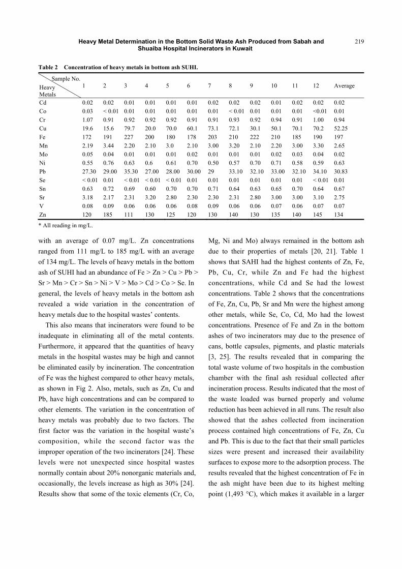
Table 2 Concentration of heavy metals in bottom ash SUHI.

Sample No.

Heavy Metals

1 2 3 4 5 6 7 8 9 10 11 12 Average

Cd 0.02 0.02 0.01 0.01 0.01 0.01 0.02 0.02 0.02 0.01 0.02 0.02 0.02

Co 0.03 < 0.01 0.01 0.01 0.01 0.01 0.01 < 0.01 0.01 0.01 0.01 <0.01 0.01

Cr 1.07 0.91 0.92 0.92 0.92 0.91 0.91 0.93 0.92 0.94 0.91 1.00 0.94

Cu 19.6 15.6 79.7 20.0 70.0 60.1 73.1 72.1 30.1 50.1 70.1 70.2 52.25

Fe 172 191 227 200 180 178 203 210 222 210 185 190 197

Mn 2.19 3.44 2.20 2.10 3.0 2.10 3.00 3.20 2.10 2.20 3.00 3.30 2.65

Mo 0.05 0.04 0.01 0.01 0.01 0.02 0.01 0.01 0.01 0.02 0.03 0.04 0.02

Ni 0.55 0.76 0.63 0.6 0.61 0.70 0.50 0.57 0.70 0.71 0.58 0.59 0.63

Pb 27.30 29.00 35.30 27.00 28.00 30.00 29 33.10 32.10 33.00 32.10 34.10 30.83

Se < 0.01 0.01 < 0.01 < 0.01 < 0.01 0.01 0.01 0.01 0.01 0.01 0.01 < 0.01 0.01

Sn 0.63 0.72 0.69 0.60 0.70 0.70 0.71 0.64 0.63 0.65 0.70 0.64 0.67

Sr 3.18 2.17 2.31 3.20 2.80 2.30 2.30 2.31 2.80 3.00 3.00 3.10 2.75

V 0.08 0.09 0.06 0.06 0.06 0.08 0.09 0.06 0.06 0.07 0.06 0.07 0.07

Zn 120 185 111 130 125 120 130 140 130 135 140 145 134

* All reading in mg/L.

with an average of 0.07 mg/L. Zn concentrations

ranged from 111 mg/L to 185 mg/L with an average

of 134 mg/L. The levels of heavy metals in the bottom

ash of SUHI had an abundance of Fe > Zn > Cu > Pb >

Sr > Mn > Cr > Sn > Ni > V > Mo > Cd > Co > Se. In

general, the levels of heavy metals in the bottom ash

revealed a wide variation in the concentration of

heavy metals due to the hospital wastes’ contents.

This also means that incinerators were found to be

inadequate in eliminating all of the metal contents.

Furthermore, it appeared that the quantities of heavy

metals in the hospital wastes may be high and cannot

be eliminated easily by incineration. The concentration

of Fe was the highest compared to other heavy metals,

as shown in Fig 2. Also, metals, such as Zn, Cu and

Pb, have high concentrations and can be compared to

other elements. The variation in the concentration of

heavy metals was probably due to two factors. The

first factor was the variation in the hospital waste’s

composition, while the second factor was the

improper operation of the two incinerators [24]. These

levels were not unexpected since hospital wastes

normally contain about 20% nonorganic materials and,

occasionally, the levels increase as high as 30% [24].

Results show that some of the toxic elements (Cr, Co,

Mg, Ni and Mo) always remained in the bottom ash

due to their properties of metals [20, 21]. Table 1

shows that SAHI had the highest contents of Zn, Fe,

Pb, Cu, Cr, while Zn and Fe had the highest

concentrations, while Cd and Se had the lowest

concentrations. Table 2 shows that the concentrations

of Fe, Zn, Cu, Pb, Sr and Mn were the highest among

other metals, while Se, Co, Cd, Mo had the lowest

concentrations. Presence of Fe and Zn in the bottom

ashes of two incinerators may due to the presence of

cans, bottle capsules, pigments, and plastic materials

[3, 25]. The results revealed that in comparing the

total waste volume of two hospitals in the combustion

chamber with the final ash residual collected after

incineration process. Results indicated that the most of

the waste loaded was burned properly and volume

reduction has been achieved in all runs. The result also

showed that the ashes collected from incineration

process contained high concentrations of Fe, Zn, Cu

and Pb. This is due to the fact that their small particles

sizes were present and increased their availability

surfaces to expose more to the adsorption process. The

results revealed that the highest concentration of Fe in

the ash might have been due to its highest melting

point (1,493 °C), which makes it available in a larger


220

Fig. 2 Average concentration of heavy metals in bottom ash of incinerators.

Table 3 Comparison of parameters of bottom ash of hospital incinerators with published results and EPA TCLP levels.

Heavy metals SAHI (a) SUHI (a) Sabah (b) Ben-Sina (b) Psychological (b) Regulated levels for toxicity of heavy metals (c)

Cd 0.01-0.03 0.01-0.02 2.0-10.0 1.0-56.0 2-16. 1.0

Co 0.06-0.08 < 0.01-0.03 NR NR NR NR

Cr 4.58-4.10 0.91-1.07 200-667 100-2,000 183-633 5.0

Cu 6.15-7.50 15.6-79.7 150-687 138-1,998 208-2,034 NR

Fe 46.9-191 127-227 727-8,867 1,167-5,700 4,233-1,233

Mn 1.10-1.24 2.10-3.44 127-597 31-328 99-389 NR

Mo 0.06-0.08 0.01-0.05 NR NR NR NR

Ni 0.08-0.12 0.55-0.76 24-41 25-141 21-52 NR

Pb 7.09-8.58 27.0-35.3 601-2,940 192-5,866 815-2,305 5.0

Se < 0.01-0.01 <0.01-0.01 NR NR NR 1.0

Sn 0.26-0.27 0.60-0.72 NR NR NR NR

Sr 3.55-4.20 2.30-3.18 NR NR NR NR

V 0.10-012 0.06-0.09 NR NR NR NR

Zn 120-194 111-185 730-6,800 827-27,800 -16,067 NR

* Note: (a) This study; (b) [3]; and (c) [26].

0.02

0.07

4.426.42

163

1.13

0.070.09

7.47

0.01

0.26

3.77

0.12

175

0.02

0.01

0.94

52.25

197

2.65

0.02

0.63

30.83

0.01

0.67

2.75

0.07

134

0.001

0.011

0.101

1.001

10.001

100.001

1000.001

Cd Co Cr Cu Fe Mn Mo Ni Pb Se Sn Sr V Zn

SAHI Incinerator

SUHI Incinerator


221

amount in the bottom ashes. When the levels of heavy

metal of this study were compared with published data,

it was found that the existing incinerators'

performances were much better than previously, as

shown in Table 3.

It seemed likely that both SAHI and SUHI

incinerators had high efficiency to reduce the heavy

metals. This means that the incinerator performance

depends entirely on the combustion degrees. To

classify the produced bottom ash from the two

incinerators as hazardous or not, toxicity characteristic

leaching procedure and characteristic waste Toxicity

Characteristic Leaching Procedure (TCLP) list was

applied [26]. According to the TCLP guidelines,

results showed that Cd, Cr and Se had a lower

concentration than TCLP. But Pb concentration was

found to have exceeded the permissible limits. Due to

Pb toxicity, the bottom ash is considered hazardous

waste, as shown in Table 3. Therefore, the produced

bottom ash from the two incinerators may be

classified as hazardous wastes, and care should be

taken during dumping [25, 27, 28]. Otherwise, it can

cause problems to the surrounding environment [29,

30]. Therefore, utilization of bottom ash is much safer

than dumping it in landfill sites [31-33].

4. Conclusions

The results of this study demonstrated that

incineration is the best technology to destroy the

increasing volume of hospital wastes. Hospital

incinerators do not completely destroy heavy metals,

but simply concentrate them into bottom ash. Bottom

ash residues arising from both incinerators were found

to contain high concentrations of hazardous elements,

such as Cd, Co, Cr, Cu, Fe, Mn, Mo, Ni, Pb, Se, Sn,

Sr, V and Zn. However, the performances of both

incinerators were much better than previously. Fe, Zn,

Pb and Cu were found in the bottom ashes of two

hospital incinerators. They were in high

concentrations compared to other heavy metals found

in the bottom ashes. Moreover, the highest melting

points of some heavy metals mean a larger amount of

their residues. The average concentrations of Pb were

found to be higher than TCLP; therefore, bottom ashes

could be classified as hazardous waste on most

sampling days. It is likely to have highly mobile

constituents of heavy metals. If they were improperly

managed, they could contaminate the groundwater.

Therefore, it is recommended that more efforts are

needed to identify why bottom ashes contain high

concentrations of Fe, Zn, Pb and Cu. Hospital bottom

ashes should be disposed by properly designed

engineered treatment methods.

Acknowledgements

The author is grateful to the Kuwait Institute for

Scientific Research (KISR) management for the

financial support to conduct this project. The author

would like to express his warm thanks to Prof. Alan

Moghissi for his guidance and good comments on this

manuscript. Thanks are also due to Prof. Mohammed

Al-Sarawi, manager of Earth Sciences and

Environment Department, Kuwait University (KU),

for his critical review of the manuscript. Special

thanks go to author's laboratory staff who always kept

things running and doing analysis on time. The

author’s wishes to thank the engineers and technical

staff from the National Cleaning Company (NCC) for

their technical information and support during this

study.

References

[1] Al-Humaidan, S. M. 2006. “Ahmadi Hospital Waste Management and Health care: Workers Perception”. The Proceedings of 4th Euro-Arab Environment Conference and Exhibition. 27-29, November, State of Kuwait, 589-599.

[2] Elliott, P., Shaddick, G., and Kleinschmidt, L. 2000. “Cancer Incidence Adverse near Municipal Waste Incinerators in Great Britain.” Br. Journal Cancer 73: 702-710.

[3] Al-Meshan, M., Nasrallah, H., and Ahmed, A. 2001. “Comparative Study of Heavy Metals in Bottom Ash from Hospital Incinerators in the State of Kuwait.” Kuwait Journal of Science 28 (2): 347-857.


222

[4] Lo, H., and Liao, Y. 2007. “The Metal Leaching and Acid-neutralizing Capacity of Msw. Incinerator Ash Co-disposed with Msw. in Landfill Sites.” Journal of Hazardous Materials 142: 512-519.

[5] Gidarakos, E., Petrantonaki, M., Anastasiadou, K., and Schramm, K. 2009. “Characterization and Hazard Evaluation of Bottom Ash Produced from Incinerated Hospital Waste.” Journal of Hazardous Materials 172: 935-942.

[6] Shim, Y., Rhee, S., and Lee, W. 2005. “Comparison of Leaching Characteristics of Heavy Metals from Bottom and Fly Ashes in Korea and Japan.” Waste Management 25: 473-480.

[7] Alba, N., Gasso, S., Lacorte, T., and Baldasano, H. 1997. “Characterization of Municipal Solid Waste Incineration Residues from Facilities with Different Air Pollution Control System.” Waste Management 47: 1170-1179.

[8] Ibanez, R., Andres, A., Viguri, J. R., Ortiz, I., and Ibrabien, J. A. 2000. “Characterization and Management of Incinerator Wastes.” Journal of Hazardous Materials 15: 793: 2-5.

[9] Zhao, L., Zhang, F., Wang, W., and Zhu, J. 2009. “Chemical Properties of Heavy Metals in Typical Hospital Waste Incinerator Ashes in China.” Waste Management Journal 29 (3): 114-115.

[10] Kougemitrou, I., Godelitsas, A., Tsabaris, C., Stathopoulos, V., and Papandreou, P. 2011. “Characterization and Management of Ash Produced in the Hospital Waste Incinerator of Athens, Greece.” Journal of Hazardous Materials 187 (1-3): 421-432.

[11] Zhao, L., Zhang, F., Mengjun, L., Zhen, G. L., and Wu, D. 2010. “Typical Pollutants in Bottom Ashes from a Typical Medical Waste Incinerator.” Journal of Hazardous Materials 15 (173): 181-185.

[12] Zakaria, M., labib, O., Mohammed, M., El-Shall, W., and Hussein, A. 2005. “Assessment of Combustion Products of Medical Waste Incinerators in Alexandria.” The Journal of the Egyptian Public Health Association 80 (3-4): 407-431.

[13] Levasseur, B., Myriam, C., Jean-Francois, B., and Mercier, G. 2006. “Metals Removal from Municipal Waste Incinerator fly Ashes and Reuse of Treated Leaches.” Journal of Environmental Engineering 132 (5): 497-505.

[14] Astar, M. 1985. “Cost Estimating for Hazardous Waste Incineration.” Pollution Engineering 1: 20-25.

[15] Tessitors, J., and Frankle, C. 1988. “Incineration of Hospital Infectious Waste.” Pollution Engineering Journal 2: 82-88.

[16] Doyle, B. W., Drum, D. A., and Lauber, J. D. 1985. “The Smoldering Question of Hospital Wastes.”

Pollution Engineering 1: 35-39. [17] Timothy, A., Timothy, O., and Morenike, A. Ji. 2013.

“Heavy Metals Concentrations Around of a Hospital Incinerator and a Municipal Dumpsite in Ibadan City, South-West Nigeria.” Journal of Apply Science and Environment Management 17 (3): 419-422.

[18] Rich, C., and Cherry, K. 1989. “The Liabilities of Hospital Waste Incineration.” Pollution Engineering 1: 48-57.

[19] Shen, T. 1986. “Hazardous Waste Incineration: Emissions and Their Control.” Pollution Engineering: 1: 50-53.

[20] Belevir, H., and Moench, H. 2000. “Factors Determining the Element Behavior in Municipal Solid Waste Incinerators.” Field studies, Environment Science Technology 34: 2501-2506.

[21] Toledo, J., Corella, J., and Corella, L. 2005. “The Partitioning of Heavy Metals in Incineration of Sludge and Waste in a Bubbling Fluidized Bed, Interpretation of Results with a Conceptual Model.” Journal Hazardous material B 126: 158-168.

[22] Varian Co. 2006. “ICP-OES Spectrometers: Varian SPS3, Sample Preparation, System and Diluter, Operation Manual.” Varian Australia Pty. Australia.

[23] Water Pollution Control Federation (WPCF). 2005. “Standard Methods for the Examination of Water and Wastewater.” Test Methods, Water Pollution Control Federation, Washington, DC: WPCF.

[24] Powell, C. 1987. “Incineration of hospital wastes.” Hazardous Waste Management 37 (7): 836-839.

[25] Gautam, V., Thapar, R., and Sharma, M. 2010. “Biomedical waste Management: Incineration vs. Environmental Safety.” Indian Journal of Medical Microbiology 28 (3): 131-192.

[26] USEPA (United State Environmental Protection Agency). 2010. “Toxicity Characteristic Leaching Procedure.” Fed. Register, 51, 216 and 40642: USEPA.

[27] Nurmesniemi, R., Poykio, K., Manskinen, O. D., and Makela, M. 2012. “Comparison of the Forest Fertilizer of Fly Ash Fractions from the MW Power Plant of a Fluting Board Mill Incinerating Peat and Forest Residues.” The 27th International Conference on Solid Waste Technology and Management, March 11-14, Ph. Pa., USA, 706-716.

[28] EC. 2003. Council Decision of 19 December 202 Establishing Criteria and Procedure for the Acceptance of Waste at Landfills. Pursuant to Article 16 of and Annex II to Directive 1999/31/EC.

[29] Al-Muzaini, S., and Jacob, P. 1997. “Trace Metals in the near Shore Sediments of the Shuaiba Industrial Area of Kuwait from August 1993 to June 1994.” J. Fac. Sci. U.A.E. 9 (1): 1-10.


223

[30] Al-Muzaini, S., and Jacob, P. 1996. “The Distribution of V, Ni, Cr, Cd and Pb in Topsoil of the Shuaiba Industrial Area of Kuwait.” Environmental Toxicology and Water Quality Environment International Journal 11: 285-292.

[31] Orava, H., Nordman, T., and Kuopanportti. H. 2006. “Increase the Utilization of Fly Ash with Electrostatic Precipitation.” Mineral Engineering 19 (15):1596-1602.

[32] Pasquini, M., and Alexander, M. 2004. “Chemical Properties of Urban Waste Ash Produced by Open Burning on the Jos Plateau: Implications for Agriculture.” Science of the Total Environment 319

(1-3): 225-240. [33] Zhang, S., Yamasaki, S., and Nanzyo, M. 2002. “Waste

Ashes for Use in Agricultural Production I: Lining Effect Content of Plant Nutrients and Chemical Characteristics of Some Metals.” Science of the Total Environment 248 (1-3): 215-225.

[34] Al-Sudairawi, M., Saeed, T., Al-Rashidi, M., Yafaoui, H., Al-Shatti, A., Al-Wadi, M., Ahmed, N., Sinan, M., Al-Awadi, L., Rashad, M., and Bahaaeldien, M. 2001. Assess the Impact of Air Pollution Emitted from Medical Waste Incinerators on the Hospital Environment and the Surrounding Areas. Final report.


Green House in Semi-arid Regions of Mexico

Maria de los Angeles Rechy Carvajal1, Emil von Roth2 and Jose Alberto Murillo Rodriguez3

1. Faculty of Forestry, Universidad Autónoma de Nuevo León, Linares, Nuevo León 67700, Mexico

2. Aegis Structural Engineers, Studio City, California 91604, USA

3. Universidad Autónoma de Nuevo León, Linares, Nuevo León 67700, Mexico

Abstract: The subject structure was consisted of a proto-type house with plan dimensions of 8 m × 4 m. A variety of materials was used to the construction, with special emphasis on using environmentally friendly non-toxic materials. The structure’s core consisted of reinforced concrete frames with masonry infill walls. Inside faces of the walls and the roof’s outside face were covered with proprietary composite panels, which are manufactured with a mixture of cement, volcanic ash, and local sawmill waste. These panels were analyzed for their physical and chemical properties, as well as for their resistance to decay and insects when subjected to extreme conditions for 15 years. The panels have also shown to provide thermal insulation and nonflammable when in direct contact with fire. The roof surface was further covered with a blend of local drought-resistant succulents and cacti. This study provides a detailed review of the construction process and materials employed. Key words: Prototype house, thermal insulation, non-combustible, resistant to decay.

1. Introduction

The objective of this research was to develop a

low-cost method to improve thermal insulation for

houses located in the semi-arid Northeast of Mexico.

This research was carried out in the city of Linares, in

the state of Nuevo León, having the geographic

coordinates: 20°50′16″ N and 99°32′41″ W (Fig. 1).

According to the Köppen-Geiger climate

classification, the climate in this area is considered

semi-arid (BSh). The average annual precipitation is

600 mm/m², dropping to an average of 400 mm/m²

during dry years. Most of the precipitation takes place

during the months of May and September. This

climate has led to the formation of thorn savannahs

(known as Matorral in the Spanish language).

The region where the study was performed is rural,

which leads to the restriction of being limited to use

locally available raw material. Automated production

of lightweight pumice or wood concrete block stones

is therefore not practically feasible.

A research project carried out at the Faculty of

Corresponding author: Maria de los Angeles Rechy Carvajal, professor, research field: forestry.

Forestry of the Universidad Autónoma de Nuevo León

(Linares, Mexico) studied various locally available

materials with the intent of identifying their suitability

for thermal insulation purposes. Local availability and

material cost led to the choice of wood concrete. This

material is characterized by being nonflammable and

highly resistant to biologically induced degradation.

2. Materials

2.1 Traditional Clay Masonry Construction

The traditional construction is clay masonry based

with thatch or palm-leaf roofs. The clay masonry

bricks employed have a density of 2 g/cm³ and a

thermal conductivity of 1.20 W/(m·K). Lighter straw

clay bricks have a density of 1.6 g/cm and a thermal

conductivity of 0.80 W/(m·K). Such values do not

allow for energy-saving construction. Additionally,

clay construction requires constant maintenance to

achieve good durability.

2.2 Current Concrete Masonry Construction

Hollow concrete masonry construction with reinforced

concrete roofs has displaced the traditional building

D DAVID PUBLISHING


225

Fig. 1 Geographical location of the studied area.

method over the last few decades. This foster by the

ease of construction, durability, and speed of

construction. Concrete’s thermal conductivity λ is 2.1

W/(m·K). This results for 15 cm thick hollow concrete

masonry blocks in a thermal conductivity λ is 0.80

W/(m·K). As a result, the thermal isolation of today's

homes in the region is not good. Thermal conductivity

values are determined experimentally through hot

plate tests (Fig. 2).

Without considering thermal boundary layers, the

thermal resistance Rw/(Rwall) for these walls is

0.15/0.80 = 0.19 m²·K/W. A 12 cm thick roof has a

Fig. 2 Equipment for determination of heat transfer.

thermal resistance of Rr/(Rrof) = 0.12/2.1 = 0.06

m²·K/W. These values are too low for habitable spaces

in semi-arid regions given that minimum recommended

R-values are Rw = 0.50 m²·K/W and Rr 1.0 m²·K/W

for walls and roofs respectively. Lack of thermal

insulation makes these houses barely habitable, This

leads to high costs related to cooling and heating.

Although high-density building materials typically

exhibit high load capacities, they are also typical

characterized by low thermal insulation properties.

3. Construction Method Used

3.1 Wood Concrete as Insulating Material

The previously mentioned research led to the

selection of wood concrete as insulation material due

to local availability and low-income wages. Wood

chips needed for manufacture of this insulation

material can be procured easily at low cost. A common

concrete mixer (Fig. 3) can be used to mix the wood

chips and cement. Manufacture of insulating wall

panels is benefitted by the use of a hydraulic press or

jack. Poured-in-place roof insulation can be

compacted with a manual compactor.

3.2 Installation of Thermal Insulation

Installation of the insulation is relatively simple.

Wall panels are adhered to the interior faces of the

walls. At the roof, the insulating wood concrete layer

is placed below and prior to pouring the load-carrying

reinforced concrete plate.

Fig. 3 Small concrete mixer.


226

Fig. 4 Outside view of the prototype house.

A prototype house with an area of 4 × 8 m was built

to test the effectiveness of the wood concrete insulation

material (Fig. 4). The walls were provided with 5 cm

thick insulation panels adhered to the inside faces. The

poured-inplace roof insulation thickness was 8 cm.

(Fig. 5). Average grade wood concrete (density ρ = 0.6

g/cm³) was used to allow for installation of normal

household items (lamps, pictures, etc.).


The research results for wood concrete was

performed following DIN 4108 and DIN EN 832

(2011), being shown in Table 1.

Thermal insulation for cooled and heated houses

should provide at the exterior of the building in order

to allow for thermal inertia of the heavy concrete

construction to contribute to a balance of interior

temperatures. In buildings that are not cooled and only

heated when required, the thermal insulation should be

provided at the interior in order to take advantage of

the nocturnal fall of temperature during the Summer

and of quick heating with minimized temperature loss

during the Winter.

The thermal conductivity λ of wood concrete is

0.16 [W/(m·K)], thus resulting in a thermal resistance

for the walls of Rwall = 0.15/0.80 + 0.05/0.16 = 0.50

[m²·K/W] and for the roof of Rroof = 0.12/2.1 +

0.08/0.16 = 0.56 [m²·K/W].

The insulation provided at the walls met the

minimum requirement for habitable spaces. In contrast,

Table 1 Research results for wood concrete.

Density Compression strength Thermal conductivity

[g/cm³] MPa w/(m·K)

0.45-0.80 1.50-2.10 0.10-0.25

Fig. 5 Interior corner showing wall and roof interface.

Fig. 6 Green roof with drought-resistant plants.

the insulation at the roof required improvement. This

roof insulation improvement was achieved through a

green roof insulation layer. Detailed quantitative

information on the level of thermal insulation

provided by the green roof was not available at time of

this publication because of the large variability of

green roof assemblies and the complexity of

determining the thermal insulation achieved.

Permanent temperature controls at the interior and

exterior surfaces showed an average temperature delta

of close to 10 °C during summer months.

Reference

[1] Rechy, de. Von., Roth, M. d. l. A. 2014. “Green


227

House Construction.” The International Conference on Dryland, Deserts and Desertification. Sede Boquer. Israel.

[2] Heyer, E. 1993. Witterung und Klima. Stuttgart: Teubner Verlag.

[3] Vermosen, G. 2008. Un Plastique Nature. Belgium: Vermosen-Bonheiden.

[4] Lohmeyer, G. C. O., Bergmann, H., Post, M. 2005.

Praktische Bauphysik. Germany: Teubner Verlag Stuttgart. [5] Din 4108. 2015. Wärmeschutz in Hochbau. Berlin: Beuth

Verlag. [6] Proporowitz, H., Unruh, H. 2008:

Baubetrieb-Bauverfahren. München: Hanser Verlag. [7] Köhler, M., Barth, G., Brandwein, T. 1993.

Fassadenbegrünung und Dachbegrünung. German: Verlag Eugen Ulmer.


Factors Affecting the Ovilarval Density of Aedes Spp.

Mosquitoes in Selected Rice Fields of Muňoz, Nueva

Ecija

Jerome Cadiente Soriano and Clarissa Yvonne Jueco-Domingo

College of Veterinary Science & Medicine, Central Luzon State University, Nueva Ecija 3120, Philippines

Abstract: Variables among the macroclimate, microclimate and rice canopy categories and three other different farming systems were evaluated on their effects to the egg and larval density of Aedes spp. mosquitoes known as transmitters of animal and human diseases. No statistical difference in egg density (#eggs/mL) among farming systems (P = 0.345) were observed. However, there was significant difference in larval density (#larvae/mL) among farming systems (P < 0.001) particularly between organic and conventional farms and between organic and mixed farms at (P < 0.05). Among the variables in the macroclimate category, wind velocity and ambient temperature significantly influenced larval density in conventional farms. Among the variables in the microclimate category, water temperature significantly contributed to larval density in both the mixed and conventional farms whereas water turbidity, in conventional farms. Among the variables in the rice canopy category, the number of tillers per plant was a significant contributor to larval density in all farm types. No variable among the environmental exposure categories affected the larval density in organic farms.

Key words: Mosquito larval control, farming system, ovilarval density, organic farming, Aedes Spp. Mosquito.

1. Introduction

Mosquitoes serve as transmitters of human and

animal diseases. The increasing trend of mosquito borne

diseases remains a challenge to national and international

health agencies to implement strategies to control it.

Some of the known diseases are yellow fever,

encephalitis, dengue, and dirofilariasis, fowl pox [1].

Vector control is an important strategy known to

enhance the sustainability of high drug coverage. It

helps interrupt transmission in combination with mass

drug administration particularly in high risk,

peri-urban areas and prevent-re-establishment of

transmission in vulnerable areas [2].

From the global standpoint, approximately 140

million hectares of land are annually devoted to rice

cultivation. Because the rice fields are flood on a

semi-permanent basis during each growing season,

Corresponding author: Clarissa Yvonne Jueco-Domingo,

Ph.D., main research field: parasitology.

they provide ideal breeding habitat for a number of

potential vectors of vector borne diseases [3].

Natural environment such as the interaction

between temperature, rainfall or variations in daily

microclimates may be important determinants in

density of eggs and larvae of mosquitoes in breeding

sites. These are very important factors in the

identification of key vector-breeding sites and the

reason is they are mosquito productive.

By determining environmental factors that

influence density of eggs and larvae of Aedes spp.

mosquitoes in three different rice farm systems in the

Science City of Muñoz Nueva Ecija namely, pure

organic, mixed and conventional farming, farmers

could be advised to be on the look out for the density

of mosquito eggs and larvae in order to make them

responsible for adopting modified human behaviors

that would protect them, their family and even their

livestock reared around their farms against the bites of

mosquitoes.

D DAVID PUBLISHING

Factors Affecting the Ovilarval Density of Aedes Spp. Mosquitoes in Selected Rice Fields of Muňoz, Nueva Ecija

229

Hence, the study determined the presence of

association between environmental factors together

with the different rice farm systems being adopted by

rice farmers in the Science City of Muñoz, Nueva

Ecija and the egg and larval density of Aedes spp. of

mosquitoes. Specifically, the study determined whether

the following environmental factors affected the egg

and larval density of Aedes spp. mosquito: (1) types of

farming systems namely organic, mixed and

conventional farms; (2) macroclimate factors such as

rainfall, humidity, ambient temperature and wind

velocity; (3) microclimate factors such as water

temperature, water pH and water turbidity; and (4)

rice canopy factors such as rice height (cm), number

of tillers per rice plant and number of panicles per rice

plant. Likewise, the study predicted egg and larval

densities of Aedes spp. mosquitoes using multiple

logistic regression models computed from environmental

factors found to be effect modifiers at (p < 0.05).

2. Material and Methods

2.1 Identification and Collection of Samples

Three organic, three mixed and three conventional

rice farms were identified within the Science City of

Munoz, Nueva Ecija for sampling collection through

the assistance of the Philippine Rural Reconstruction

Movement farmers’ cooperative. External in puts such

as herbicides, fertilizers and pesticides applied on the

rice fields by farmers were noted.

Evaluation of rice plants and collection of water

samples with mosquito eggs and larvae were done

from three different sites of each rice field as

replicates. Duration of collection period for the entire

study was two months with weekly collections for a

total of eight (8) collections.

2.2 Gathering of Macroclimate Variables

Macroclimate variables include meteorological

factors such as ambient temperature (oC), humidity

(%), wind velocity (mps) and rainfall (mm). They

were taken from the Agrometeorological office of the

Dept. of Agronomy, Philippine Rice Research

Institute in Maligaya, Science City of Munoz and

Nueva Ecija.

2.3 Gathering of Characteristics of Rice Paddy Water

Around fifty (50) milliliters (mL) of water from the

rice paddies were collected and placed in clean

properly labeled plastic bottles. Samples from the

water were submitted for pH and water turbidity

analysis at the Philippine Rice Institute Department of

Agronomy. The pH was measured using a pH meter

while the water turbidity was analyzed using

spectrophotometric measurement for light absorbance

(nanometer). Water temperature was measured from

all sample sites using the Field Environmental

Thermometer.

2.4 Evaluation of Rice Canopy Development

All rice plants within the area of one by one square

meter, also designated for collection site of water

sample, which was evaluated for rice canopy factors:

1. Plant height in centimeters (cm)-taken from the

base of the plant which was submerged in water until

the highest tip of the plant. A meter stick was used for

measuring;

2. Number of tillers per plant-number of culmns or

tillers was counted per plant and the mean per

sampling site was recorded;

3. Number of panicles per plant-number of panicles

was counted per plant and the mean per sampling site

was recorded.

2.5 Identification & Counting of Eggs and Larvae of

Aedes spp. Mosquitoes

Three (3) different collection sites for each type of

rice farm were sampled for water to determine the

number of eggs and larvae. Each site was marked with

a flag to identify the area for collection throughout the

study period.

Around 240 mL of water with eggs and larvae was

collected from each replicate site and placed in


230

chemically clean bottles. An aliquot of ten 10 mL was

transferred to a vial and a thin layer of mineral oil was

placed over the surface of the water sample to

suffocate the larvae. After the larvae have been killed,

the entire contents of the vial were poured into a Petri

dish and the eggs and larvae were counted using

magnifying lens.

Only Aedes spp. mosquito eggs that were laid

singly and did not have lateral floats were counted.

The larvae that hanged diagonally from the water

surface were assumed to be Aedes spp. Although

Culex spp. also has larvae that hang diagonally from

the water surface, the females prefer to lay eggs in

stagnant, dirty water as compared to Aedes spp. that

lay eggs in rice paddies.

Egg density per milliliter was computed by number

of eggs counted divided by 10 mL while larval density

per mL was measured by the number of larvae

counted divided by 10 mL. Values of the egg and

larval densities were transmuted according to the area

of the entire rice field.

2.6 Data Analysis

Mean scores of the replicates of each rice farm were

computed. One-way analysis of variance was used to

evaluate the significant difference of the different

environmental exposure variables by farm and the

significant difference of mean egg and larval densities

by farm.

Multivariate analysis was done to assess the

association of exposure variables grouped in

categories or as individual entity to the mean egg

density or mean larval density. Each category, for

instance, macroclimate, microclimate and plant

canopy was forced into a multiple logistic regression

model. A regression model per category was created

which served as the main effects model. Each

exposure variable under that category was assessed on

how it interacted to the main effects model. The

category which had a log likelihood ratio p-value of

less than 0.05 was considered an effect measure

modifier. Hence, it could significantly modify either

the mean egg density or the mean larval density.

Similarly, individual exposure variables were

subjected to multivariate analysis to assess their

association to the mean egg density or mean larval

density. Each exposure variable was forced into a

multiple logistic regression model. An exposure

variable which had a log likelihood ratio p-value of

less than 0.05 was considered an effect measure

modifier, hence, it could significantly modify either

the mean egg density or the mean larval density.


Comparing the summation of the mean egg density

(#eggs/mL) and larval density in organic, mixed and

conventional farms, ANOVA showed no significant

difference at (p = 0.345) in the egg density while

larval density was significantly different among the

farming systems at (p < 0.001) (Table 1). This implies

that the water paddies in mixed and conventional

farms are better culture grounds for sustaining larval

development. On the other hand, water paddies of

organic farms are least attractive for sustaining larval

density.

Likewise, results imply that egg density is not a

good monitoring index for mosquito density in

evaluating strategies for integrated vector control

management program since there is no difference in

the density among farms despite of a significant

difference in the larval density. Hence, between egg

and larval density, the latter is more sensitive as

environmental index for monitoring mosquito density.

Table 1 Analysis of variance of the summation of the mean egg and larval density by farming system.

Egg density (No.eggs/mL)

Larval density (No.larva/mL)

Organic 1,730 a 2,711 a

Mixed 2,093 a 5,229 b

Conventional 2,651 a 7,590 c

P value 0.345 ns 0.000 **

* ns-not significant (similar superscripts are not significantly different); ** highly significant.


231

Table 2 shows the crude analysis of environmental

exposure categories by farm type to identify which

one would be an effect modifier (p < 0.05) to egg

density of Aedes spp. Macroclimate variables

include the ambient temperature (oC), humidity (%),

wind velocity (mps) and rainfall (mm). Results

showed that only the macroclimate had a moderate

modifying effect at p = 0.05 to egg density in organic

farms. In the case of mixed farms, no environmental

exposure category had any association with egg

density while the microclimate category had a

modifying effect at p = 0.002 to egg density in

conventional farms. Microclimate variables include

those which characterize the water quality of the rice

paddies such as water pH, water temperature and

water turbidity.

When taken individually (Table 3), the wind was a

significant contributor under the macroclimate

category at p = 0.031 in organic farms while it was the

ambient temperature at p = 0.008 in conventional

farms. The water temperature under the microclimate

category was a significant contributor to egg density at

p = 0.019 in mixed farms and p = 0.000 in

conventional farms.

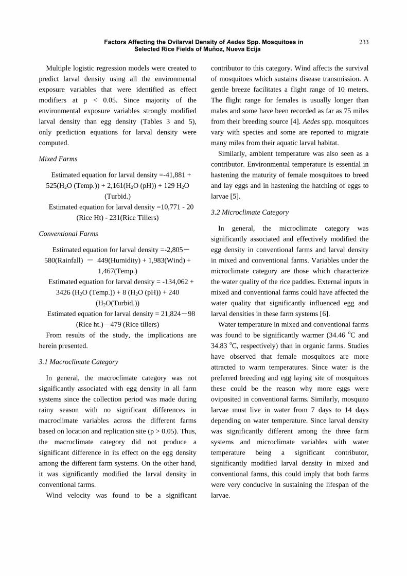
Table 4 shows the crude analysis of environmental

exposure categories by farm type to identify which

one would be an effect modifier (p < 0.05) to larval

density of Aedes spp. Results showed that no

environmental exposure category had a modifying

effect to larval density in organic farms. However, the

microclimate category was an effect modifier at p =

0.031 in mixed farms whereas all environmental

exposure categories were effect modifiers to larval

density in conventional farms.

Table 2 Multivariate analysis of environmental exposure categories by farm type against egg density of Aedes spp.

Organic farm Mixed farm Conventional farm

Macroclimate 0.05* 0.123 0.057

Microclimate 0.561 0.109 0.002**

Plant canopy 0.679 0.116 0.488

*significant; **highly significant.

Table 3 Significant exposure variables to mean Egg Density (ED).

p-Value < 0.05 (effect modifier)

Organic farms Mixed farms Conventio-nal farms

Macroclimate category 0.05 0.123 0.057

Wind (mps) 0.031* 0.134 0.782

Rainfall (mm) 0.730 0.096 0.600

Humidity (%) 0.203 0.060 0.633

Ambient temp. (oC) 0.561 0.850 0.008*

Microclimate category 0.561 0.109 0.002*

Water pH 0.953 0.293 0.760

Water temp. (oC) 0.304 0.019* 0.000*

Water turbidity (nm) 0.447 0.604 0.251

Rice canopy category 0.679 0.116 0.488

Plant height (cm) 0.414 0.678 0.442

No. of tillers/plant 0.401 0.442 0.406

No. of panicles/plant 0.418 n.a. 0.395

* na-not applicable; *statistically significant.


232

Table 4 Multivariate analysis of environmental exposure variables by farm type against larval density of Aedes spp.

Organic farm Mixed farm Conventional farm

Macroclimate 0.342 0.511 0.000**

Microclimate 0.302 0.031** 0.000**

Plant canopy 0.059 0.054 0.000**

*significant; **highly significant.

When taken individually (Table 5), the wind velocity

and ambient temperature strongly contributed to the

macroclimate category in affecting the larval density

in conventional farms at p = 0.030 and p = 0.004

respectively. Water temperature and water turbidity

strongly contributed to the microclimate category in

affecting the larval density in conventional farms at p

= 0.000 and p = 0.019 respectively. Finally, the

number of tillers per plant strongly contributed to rice

canopy category in affecting the larval density in

conventional farms at p = 0.04. Rice canopy indicators

include plant height (cm), the number of tillers per

plant and number of panicles per plant.

Table 6 shows the analysis of variance of the mean

values of individual exposure variables by farm type.

Water temperature, water pH, number of tillers and

panicles per rice plant significantly differed by farm

system whereas, water turbidity and plant height were

not significantly different at p = 0.115 and p = 0.766

respectively, significantly by farm type.

Table 5 Significant exposure variables to mean Larval Density (LD).

p-value < 0.05 (effect modifier)

Organic farms Mixed farms Conven-tional farms

Macroclimate category 0.342 0.511 0.000*

Wind (mps) 0.249 0.111 0.030*

Rainfall (mm) 0.164 0.293 0.078

Humidity (%) 0.426 0.233 0.126

Ambient temp. (oC) 0.376 0.939 0.004*

Microclimate category 0.302 0.031* 0.000*

Water pH 0.065 0.228 0.997

Water temp. (oC) 0.477 0.057 0.000*

Water turbidity (nm) 0.878 0.211 0.019*

Rice canopy category 0.059 0.054 0.000*

Rice plant height 0.374 0.953 0.565

No. of tillers/plant 0.158 0.646 0.04*

No.of panicles/plant 0.064 n.a. n.a.

* na-not applicable; *statistically significant

Table 6 Comparison of mean values of environmental exposure variables by farm systems.

Organic farms Mixed farms Conventio-nal farms p-value

Mean H2O temp. (To) 33.87 34.46 34.83 0.002**

Mean H2O pH 7.790 7.754 7.521 0.002**

Mean H2O turbidity 88.58 90.514 91.162 0.115ns

Mean rice ht. (cm) 34.26 35.37 35.65 0.766ns

Mean no. of tillers/plant 33.00 27.97 29.45 0.002**

Mean no. of panicles/plant 296 293 341 0.04**

* ns-not significant; ** means highly significant.


233

Multiple logistic regression models were created to

predict larval density using all the environmental

exposure variables that were identified as effect

modifiers at p < 0.05. Since majority of the

environmental exposure variables strongly modified

larval density than egg density (Tables 3 and 5),

only prediction equations for larval density were

computed.

Mixed Farms

Estimated equation for larval density =-41,881 +

525(H2O (Temp.)) + 2,161(H2O (pH)) + 129 H2O

(Turbid.)

Estimated equation for larval density =10,771 - 20

(Rice Ht) - 231(Rice Tillers)

Conventional Farms

Estimated equation for larval density =-2,805－

580(Rainfall) － 449(Humidity) + 1,983(Wind) +

1,467(Temp.)

Estimated equation for larval density = -134,062 +

3426 (H2O (Temp.)) + 8 (H2O (pH)) + 240

(H2O(Turbid.))

Estimated equation for larval density = 21,824－98

(Rice ht.)－479 (Rice tillers)

From results of the study, the implications are

herein presented.

3.1 Macroclimate Category

In general, the macroclimate category was not

significantly associated with egg density in all farm

systems since the collection period was made during

rainy season with no significant differences in

macroclimate variables across the different farms

based on location and replication site (p > 0.05). Thus,

the macroclimate category did not produce a

significant difference in its effect on the egg density

among the different farm systems. On the other hand,

it was significantly modified the larval density in

conventional farms.

Wind velocity was found to be a significant

contributor to this category. Wind affects the survival

of mosquitoes which sustains disease transmission. A

gentle breeze facilitates a flight range of 10 meters.

The flight range for females is usually longer than

males and some have been recorded as far as 75 miles

from their breeding source [4]. Aedes spp. mosquitoes

vary with species and some are reported to migrate

many miles from their aquatic larval habitat.

Similarly, ambient temperature was also seen as a

contributor. Environmental temperature is essential in

hastening the maturity of female mosquitoes to breed

and lay eggs and in hastening the hatching of eggs to

larvae [5].

3.2 Microclimate Category

In general, the microclimate category was

significantly associated and effectively modified the

egg density in conventional farms and larval density

in mixed and conventional farms. Variables under the

microclimate category are those which characterize

the water quality of the rice paddies. External inputs in

mixed and conventional farms could have affected the

water quality that significantly influenced egg and

larval densities in these farm systems [6].

Water temperature in mixed and conventional farms

was found to be significantly warmer (34.46 oC and

34.83 oC, respectively) than in organic farms. Studies

have observed that female mosquitoes are more

attracted to warm temperatures. Since water is the

preferred breeding and egg laying site of mosquitoes

these could be the reason why more eggs were

oviposited in conventional farms. Similarly, mosquito

larvae must live in water from 7 days to 14 days

depending on water temperature. Since larval density

was significantly different among the three farm

systems and microclimate variables with water

temperature being a significant contributor,

significantly modified larval density in mixed and

conventional farms, this could imply that both farms

were very conducive in sustaining the lifespan of the

larvae.


234

Table 7 Summary of regression analysis on larval density in mixed farms based on microclimate variables.

Predictor Coef. St Dev.

T-stat P value

Constant -41,881 16,904 -2.48 0.019

H2O temp. 525.2 265.8 1.98 0.057

H2O pH 2,161 1,757 1.23 0.228

H2O turbidity 129.0 100.9 1.28 0.211

* S = 3,570; R-Sq = 24.6%; R-Sq (adj) = 7.4%.

Table 8 Summary of regression analysis on larval density in mixed farms based on rice canopy variables.


T-stat P value

Constant 10,771 2,815 3.83 0.001

Rice Ht -20.3 343.8 -0.06 0.953

Rice Till -231.4 498.7 -0.46 0.646

* S = 3,694; R-Sq = 16.7%; R-Sq (adj) = 11.5%.

Table 9 Summary of regression analysis on larval density in conventional farms based on macroclimate variables.


T-stat P value

Constant -2805 36,960 -0.08 0.940

Rainfall -580.3 319.8 -1.81 0.078

Humidity -448.7 285.9 -1.57 0.126

Wind velocity 1,983.3 877.6 2.26 0.030

Ambient temp. 1,467.3 477.6 3.07 0.004

* S = 4,024; R-Sq = 51.7%; R-Sq (adj) = 46.0%.

Table 10 Summary of regression analysis on larval density in conventional farms based on miroclimate variables.


T-stat P value

Constant -134,062 25,811 -5.19 0.000

H2O Temp 3,426.0 461.0 7.43 0.000

H2O pH 8 1,939 0.00 0.997

H2O Turbidity 240.36 98.01 2.45 0.019

* S = 3,203; R-Sq = 68.5%; R-Sq (adj) = 65.8%.

Table 11 Summary of regression analysis on larval density in conventional farms based on microclimate variables.


T-stat P value

Constant 21,824 1,612 13.54 0.000

Rice Ht -97.9 168.8 -0.58 0.565

Rice Till -479.4 225.0 -2.13 0.040

*S = 2,993; R-Sq = 71.7%; R-Sq (adj) = 70.1%.

Water turbidity was found to significantly modify

the larval density in conventional farms. Water

turbidity is a consequence of fertilizer application.

Fertilizers contain nitrogen, phosphorus and

potassium [7]. Microorganisms in the soil decompose

them in order to release the nutrients needed by the

plants. Sources of organic fertilizers are green manure

composed of decaying vegetation, crop residue or rice

straw and animal manure. It takes three days for green

manure to be decomposed, one month for crop residue


235

and one week for animal manure. Whereas, inorganic

fertilizers were being used in conventional farms take

two to three weeks. In this study, fertilizers used by

organic farms were processed poultry manure while

mixed and conventional farms utilized inorganic

fertilizer (registered brand name “Crop Giant

15-15-30”) [7].

Water samples were analyzed for the presence of

microscopic organisms. Results revealed the presence

of filamentous green algae such as Oedogonium,

Microspora and Zygnemopsis. Simple blue-green

algae and filamentous blue-green algae were also

found such as Rivularia and Oscillatoria, respectively.

Likewise, unicellular zooflagellates such as

Euglenoids, Ciliates (Paramecium, Colpoda) and

Rotifers were seen.

Usually, fertilizers are applied in the flooded fields

before transplanting the rice. Since inorganic

fertilizers take a long time to be decomposed by the

microorganisms, the presence of nitrogen, phosphorus

and potassium in the water increase the growth of

green and blue green algae that supply the food chain

of mosquito larvae for their growth and development

[4]. In addition, presence of these algae also supports

the life of zooflagellates that also add to the water

turbidity [7].

3.3 Rice Canopy Category

In general, rice canopy category significantly

modified the larval density only in conventional farms.

Specifically, the number of tillers per plant

significantly contributed to the category. Number of

tillers per plant serves as plant canopy for resting sites

and protection from adverse elements including high

temperature, low humidity and heavy winds. After

feeding, female mosquitoes seek out resting places.

After digesting the blood meal, the adult will oviposit

in an appropriate habitat. Washino and Wood [8]

studied characteristics of land cover in California

which were dominated by low mosquito producing

rice fields and high mosquito producing rice field

using remote sensing. Probability of females

completing the gonotrophic cycle could be estimated

by the state of vegetation canopy development of the

potential habitat.

3.4 Other Findings

Plenty of livestock that grazed around the farms

were observed of which, the nearest grazing distance

from the perimeter of the rice paddies was 30 meters.

These animals were goats, swamp buffaloes, cattle,

free range chickens and ducks. Similarly, residents

around the farms also engaged in backyard piggeries.

Other domestic animals living near the farms were

dogs and cats.

The presence of livestock occupying the pastures

near the rice paddies provides a dynamic support to

Aedes spp. mosquito population. Soon after adult

female mosquitoes emerge from the rice fields they

will seek sources of blood meal to nourish their eggs

after mating [9]. Since livestock is always available

anytime as blood meal for these mosquitoes, there will

always be eggs laid and larvae maintained until they

develop into adults in the water paddies of these farms

that have particular characteristics in their

microclimate and rice canopy variables that support

the life cycle of Aedes spp. mosquitoes [8].

In addition, Aedes spp. mosquitoes are mechanical

or biological vectors of a number of diseases affecting

animals such as dirofilariasis and fowl pox and a

number of zoonotic pathogens that are transmitted to

humans from animal reservoirs such as arboviruses

causing encephalitis aside from the known human

disease such as Dengue. Hence, the presence of

livestock adds to the maintenance cycle of pathogens

transmitted by Aedes spp. mosquitoes.

4. Conclusion

Larval density is a good monitoring index for

mosquito density in evaluating environmental indices

for integrated vector control. Rice paddies in mixed

and conventional farms are better density culture


236

grounds for sustaining larval development than

organic farms. The variables were found to be

significant contributor in influencing the larval density

in mixed and conventional farms: macroclimate

category with wind velocity & ambient temperature

variables, microclimate category with water

temperature & water turbidity and rice canopy

category with rice height and number of tillers per

plant as variables.

For mixed farms, a regression equation model using

variables under microclimate category and rice canopy

were created to predict larval density. For

conventional farms, equation models using variables

under the macroclimate, microclimate and rice canopy

categories were created to predict larval density. No

environmental exposure variables were identified as

effect modifiers for larval density in organic farms.

References

[1] Gubler, D. J., Edward, B., and Hayes, M. D. 1992. “Dengue and Dengue Hemorrhagic Fever.” Accessed May 19, 1992.

http:/wonder. Cdc.gov/wonder/prevgid/p0000373.asp. [2] WHO., Media. Centre. 2002. “Disease Outbreak News.

Dengue fever, Dengue hemorrhagic fever.” WHO Fact Sheet. Accessed May 19, 2006. http://www.who.int/csr/diseasedengue/en.html.

[3] Falcon, T. 2005. “Water Management in Rice in Asia.” Accessed June 2, 2006. http:/www.fao.org/documents.

[4] Belding, D. L. 1964. Textbook of Parasitology. 3rd Edition. New York: Appheton-Century-Cofts, 802, 872, 684.

[5] Chandler, A. C. and C. P. 1961. Introduction to Parasitology 10th Edition. New York: John Wiley and Sons Incorporated. 730, 743, 750.

[6] Rice as a Plant: Growth Phases. 2002. “In Ricepedia, the Online Authority on Rice.” Accessed June 2, 2006. https:ciat.cgiar.org/crops/rice.

[7] Javier, E., and Rodante, T. 2003. “Nitrogen Dynamics in Soils Amended with Different Organic Fertilizers.” Phil. J. Crop Sci. 28 (3): 49-60.

[8] Washino, R. K., and Byron, L. W. 1994. “Application of Remote Sensing to Vector Arthropod Surveillance and Control.” American Journal of Tropical Medicine and Hygiene 50: 134-144.

[9] Barrinuevo, G. L., and REY, L. E. 2005. “DOH Warns of Dengue Outbreak.” Accessed May 19, 2006. http://www.manilatimes.net/national/2005/aug/09/yehey/life/20050809lif3.html.


Decommissioning of Uranium Pilot Plants at

IPEN-CNEN/SP: Facilities Dismantling, Decontamination

and Reuse as New Laboratories for Strategic Programs

Paulo Ernesto de Oliveira Lainetti1, Antônio Alves de Freitas1, Francisco Mário Feijó Vasques2 , Robson de Jesus

Ferreira2, Marycel Elena Barbosa Cotrim1 and Maria Aparecida Faustino Pires1

1. Instituto de Pesquisas Energéticas e Nucleares-IPEN-CNEN/SP, National Nuclear Energy Commission-CNEN, C. Universitária,

Butantã, São Paulo-SP, CEP 05508-000, Brazil

2. Instituto de Pesquisas Energéticas e Nucleares-IPEN-CNEN/SP, National Nuclear Energy Commission-CNEN, C. Universitária,

Butantã, São Paulo CEP 05729-090, Brazil

Abstract: From beginning of 90’s, the Brazilian nuclear policy has been changed radically. This determined the interruption of most R&D fuel cycle activities and the facilities shutdown at Nuclear and Energetic Research Institute (IPEN). The existence of those facilities also implicated in the need of constant surveillance, representing additional obligations, costs and problems. The reasons to promote the dismantling of the IPEN’s Nuclear Fuel Cycle Pilot Plants elapsed mainly from the need of physical space for new activities, since the R&D in the nuclear fuel cycle area were interrupted. In the last decade, IPEN has changed its “nuclear profile” to a “comprehensive and multidisciplinary profile”. With the end of most nuclear fuel cycle activities, the former facilities were distributed in four different centers. Each center has adopted a different strategy and priority to face the D&D problem. The available resources depend on the specific program in each area’s development (resources available from other sources, not only from Brazilian National Nuclear Energy Commission (CNEN). One of those new activities is the IPEN’s Environmental Program. This paper describes the procedures, problems faced and results related to the reintegration of the former pilot plant areas as new laboratories of the Chemical

and Environmental Technology CenterCQMA of the IPEN.

Key words: Decommissioning, dismantling, decontamination, pilot plants, reuse.

1. Introduction

Radical changes of the Brazilian nuclear policy, in

the beginning of 90’s, determined the interruption of

most R&D fuel cycle activities and the facilities

shutdown at IPEN. Those facilities already played their

roles of technological development and personnel's

training, with transfer of the technology for institutions

entrusted of the “scale up” of the units. Most of the

pilot plants had the activities interrupted until

1992-1993, due to the lack of resources for the

continuity of the research. The appropriate facilities

Corresponding author: Paulo Ernesto Oliveira Lainetti,

Ph.D., main research field: thermal treatment of wastes and nuclear materials.

maintenance has been also harmed by the lack of

resources, with evident signs of deterioration in

structures and equipments. The existence of these

facilities also implicates in the need of constant

surveillance, representing additional obligations, costs

and problems.

Since then, IPEN has faced the problem of facilities

dismantling and/or decommissioning. Immediately

after the nuclear R&D program interruption, the

uncertainties related to an eventual retaking of the

program created some political hesitation about the

dismantling decision. As the retaking of the R&D

Nuclear Program is now discarded, the

decommissioning seems to be the obvious choice. The

decommissioning strategy for the old facilities

D DAVID PUBLISHING

Decommissioning of Uranium Pilot Plants at IPEN-CNEN/SP: Facilities Dismantling, Decontamination and Reuse as New Laboratories for Strategic Programs

238

dedicated to the technological domain of the Nuclear

Fuel Cycle follows an approach of advancing gradually

in dismantling, since the resources and technical

conditions are available.

2. Reasons and Priorities for Dismantling and Decommissioning

The reasons of such approach are the need of

political decisions related to the destiny of the facilities,

lack of financial resources and of specialized personnel

in the decommissioning issue, besides the fact that

decommissioning is not an institutional priority in the

present. As some facilities had the activities suspended

for about twelve to fifteen years, also constitute

relevant problems the equipment deterioration and

personnel's loss, due retirements and transfers for other

activities and increasing difficulties related to the

availability of operational reports, drawings and

descriptive memorials.

Some factors affecting the decision and the strategy

of dismantling and decommissioning should be

mentioned: the IPEN is located in the Sao Paulo City,

in the Campus of Sao Paulo University, in an area of

nearly 500,000 square meters; the space occupied by

the old facilities constitutes a very valuable area;

nowadays, the surroundings are a very populated area,

in opposition to the past (when the facilities were built);

the localization is an important aspect determining the

reuse of the space and buildings of the former fuel

cycle facilities.

Besides this, the reasons to promote the dismantling

of the IPEN’s Nuclear Fuel Cycle Pilot Plants as soon

as possible elapses of three main aspects: need of

physical space for new activities and priorities as, for

example, the Fuel Cells Program, since the activities of

R&D in the area of the nuclear fuel cycle were

interrupted, not having perspectives of retaking of the

Program; need to take advantage, as soon as possible,

of the researchers’ knowledge, mainly from those were

indeed involved with the project, assembly and

operation of the different facilities, since it comes

happening a gradual loss of personnel for retirements

and transfers; the long period since the interruption of

the activities in above mentioned facilities has been

taking to an increase in the difficulty of tracking

documents and reliable information, besides to evident

deterioration of structures, increasing the concerns

related to the risk of liberation of radioactive

compounds and/or risks for their chemical toxicities.

On one hand, in the beginning of the activities, it was

considered the problem of the costs related to facilities

maintenance/surveillance and of the gradual loss of

knowledge accumulated (because of retirement or

dispersion of the personnel former involved with the

different nuclear fuel cycle processes). As the activities

were interrupted in most facilities, IPEN has promoted

a professional recycling of the remaining personnel

with emphasis in other Institution different priorities

such as radioisotope production or research reactor

operation and fuel production or environmental

applications of the existent experience (chemical

processes). On the other hand, there was the problem of

dismantling costs, mainly considering that there was no

experience/expertise in this field at all at IPEN.

Another problem was the evaluation of the facilities

status in terms of chemical and radiological

contamination levels for equipment/soil/buildings,

after more than ten years since the facilities shutdown.

Last, but not least, it should be mentioned the problem

of the exhausted capacity of radioactive waste storage

in the IPEN.

An aspect considered in the beginning of the

activities was the lack of experience or expertise in the

dismantling and decommissioning area at all at IPEN.

Besides this, it was necessary to recovery reliable

data/drawings about the facilities. It was very clear that

would be necessary to improve all steps involving

decommissioning, such as planning, regulatory

requirements, cost estimating, cost-benefit analysis,

need for and extent of decontamination, selection of

decontamination techniques, assessment of the waste

amount from the dismantling, dismantling techniques,


239

staff training and so on.

In the last decade IPEN has changed its “nuclear

profile” to a “comprehensive and multidisciplinary

profile”. During this period, IPEN has been restructured

in 13 Research Centers. With the end of most nuclear

fuel cycle activities, the former facilities were distributed

in four different centers: Environmental and Chemical

Technology Center, Fuel Cell Center, Materials

Science and Engineering Center, Nuclear Fuel Center.

Each center has adopted a different strategy and

priority to face the D&D problem and to reintegrate the

areas. The resources available depend on the specific

program developed in each area (resources available

from other sources, not only CNEN). In the Fig. 1, it

can be observed the localization of the nuclear fuel

cycle facilities in the IPEN plan.

3. Reuse of Dismantled Nuclear Facilities

Some Brazilian governmental and strategic

programs are: Fuel Cells, Nanotechnology,

Biomaterials, Environment and Polymers. Considering

all aspects mentioned before, the old facilities, and the

occupied area, constitutes a significant and useful

resource, since they can be fully or partially reutilized

for a variety of purposes and programs. Besides the full

release of some facilities as “green areas” (priority

programs), some buildings can also be used as interim

storage facilities (for equipment and wastes). It should

be mentioned that the decision regarding the reuse of

the different facilities has been made on a case-by-case

basis.

In 2000/2001, it was dismantled part of Thorium and

UF4 Production (aqueous route) Pilot Plants-Building

2/CQMA and in 2002/2003 it were dismantled the

ADU Dissolution and the Uranyl Nitrate Purification

Pilot Plants-Building 1/CQMA. In the Fig. 2, some

pictures of the dismantling operations of the ADU

Dissolution and Uranyl Nitrate Purification Pilot Plants

are presented. The previous dismantling activities were

described in [1-5].

Fig. 1 Localization of the IPEN’s fuel cycle facilities (left) and the ADU dissolution and uranyl nitrate purification building (arrow).


240

Fig. 2 Some pictures of dismantling operations of the ADU dissolution and uranyl nitrate purification pilot plants.

Fig. 3 Some pictures of facility decontamination.

The ADU Dissolution and Uranyl Nitrate

Purification Pilot Plants have been reintegrated as the

new laboratories of the IPEN’s Environmental IPEN’s

program. The Thorium Pilot Plant and the UF4

Production Pilot Plant (Aqueous Route) have been

reintegrated as the new laboratories of the Polymers

Program. In the Fig. 3, some pictures of floor and walls

decontamination in the facility’s building are showed.

4. Radioactive Wastes in the Operations

The main practical difficulty associated to the task of

the dismantling and decommissioning of the old

Nuclear Fuel Cycle facilities of the IPEN was the large

amount of radioactive waste generated in the

dismantling operations. The waste was mainly in the

form of contaminated carbon steel structures. In the

IPEN, the presence of contamination in the equipments,

structures and buildings, although restricted to low and

average activity levels, constituted an important

concern due, on one hand, to the great volume of

radioactive wastes generated during the operations. On

the other hand, it should be outstanding that the

capacity of stockpiling the radioactive wastes in IPEN

found been exhausted. Basically, for the dismantling

operations of the units, the main radionuclides of

interest, from the radioprotection point of view, are U

of natural isotopic composition and the thorium-232.

Several methods have been applied for the

minimization of radioactive waste [6-10]. The choice

of a coating removal process for radioactive material in

the form of carbon steel pieces must have into account,

among other factors, that it is not necessary a high


241

quality of finishing, since the main objective is the

release of the material as iron scrap. Different from

other applications, where the main objective is to

recover the component for reworking (appliances

industry, for instance), the reduction of waste volume

and the consequent need of expensive containers and

space for storage are the driving forces.

It was decided to explore the former experience with

molten salts in the thermal decomposition of

radioactive organic wastes to investigate the possibility

of its application as a potential method to solve the

problem of the radioactive waste generated during the

dismantling operations of the Nuclear Fuel Cycle Pilot

Plants of the IPEN.

In spite of the use of molten salt has already been

developed for some industrial coating removal process,

it has not been found references in the literature about

its use for radioactive superficial contamination

removal. The molten salt stripping process relies on

chemical oxidation of the coating by a molten salt bath.

A new process for radioactive contamination removal

from metallic surfaces was developed and a patent

privilege request was submitted to analysis in the

Brazilian Industrial Property InstitutINPI: related to

the Process for Radioactive Decontamination of Parts

Components and Metallic Structures in Molten Salt

Baths

5. Conclusions

A private company was hired to the building

decontamination activities, conditioning of the

radioactive wastes and rebuilding. Beginning from the

work to the end of the task, medical examination and

clinic analysis for the personnel in charge of the job

(from hired companies), in accordance with the

requirements of IPEN. Besides this, a training of the

company team was supplied by the IPEN’s

radiological protection staff.

During the pilot plant dismantling activities a new

process for radioactive decontamination of complex

steel structures was developed [11-14]. After the

conclusion of the activities it was realized a

radioactive monitoring of the laboratories and they

were full released by Radiation Protection Area Dose

≤ 0.3 mSv.

Acknowledgments

Acknowledge the help of the several technicians

directly involved with the dismantling operations.

Acknowledge also the support of International Atomic

Energy Agency that provided funds to the Research

Project-Decommissioning of Nuclear Fuel Cycle

Facilities at IPEN (Brazil), Contract No.BRA-12800.

References

[1] Lainetti, P. E. O., Freitas, A., Ferrari, E., Ferreto, H., Ayoub, J., Seneda, J., et al. 2002. Plano de Ação Para Desmontagem das Unidades do Ciclo do Combustível. IPEN’s Internal report (in portuguese), São Paulo, February.

[2] Lainetti, P. E. O., Freitas, A. A. 2003. Desmontagem Das. Unidades de Dissolução e Purificação de Urânio do Ciclo do Combustível–Bloco I do CQMA. IPEN’s Internal report, São Paulo, March.

[3] Lainetti, P. E. O. 2005. “Decommissioning of Nuclear Fuel Cycle Facilities-IPEN’s Experience.” Proceedings of the 7th Enan International Meeting on Nuclear Applications, INAC 2005, Santos, SP, Brasil.

[4] Lainetti, P. E. O. 2005. “Decommissioning of Nuclear Fuel Cycle Facilities at IPEN (Brazil), IAEA Research Project BRA-12800.” Research Coordination Meeting Innovative and Adaptive Technologies in Decommissioning of Nuclear Facilities, Halden, Norway.

[5] Lainetti, P. E. O. 2006. “Status of the Program and Progress in R&D Activities in Support of: Decommissioning of Nuclear Fuel Cycle Facilities at IPEN (Brazil), IAEA Research Project BRA-12800.” Research Coordination Meeting Innovative and Adaptive Technologies in Decommissioning of Nuclear Facilities, Keswick, UK.

[6] Guide to Cleaner Technologies–Organic Coating Removal, EPA/625/R-93/015 Office of Research and Developmen-US EPA. Washington DC: United States Environment Protection Agency.

[7] International Atomic Energy Agency. 2001. Methods for Minimization of Radioactive Waste from Decontamination and Decommissioning of Nuclear Facilities. Technical reports Series No. 401.

[8] International Atomic Energy Agency. 2006. Management of Problematic Waste and Material Generated During the


242

Decommissioning of Nuclear Facilities. Technical Reports Series No. 441.

[9] IAEA-TECDOC-1527. 2006. Application of Thermal Technologies for Processing of Radioactive Waste. Vienna: International Atomic Energy Agency.

[10] Janz, G. J. 1967. Molten Salts Handbook, New York: Academic Press.

[11] Lainetti, P. E. O. 2010. “Molten Salts as Stripping Media for Radioactive Superficial Decontamination” Proceedings of the European Nuclear Conference Barcelona, Spain.

[12] IAEA-TECDOC-1602. 2008. Innovative and Adaptive Technologies in Decommissioning of Nuclear Facilities, Vienna: International Atomic Energy Agency.

[13] Lainetti, P. E. O. 2009. “Development of a New Process for Radioactive Decontamination of Painted Carbon Steel Structures by Molten Salt Stripping.” Proceedings of the 2009 International Nuclear Atlantic Conference-INAC.

[14] Lainetti, P. E. O. 2007. “Decommissioning of Nuclear Fuel Cycle Facilities in the IPEN-CNEN/SP.” Proceedings of the European Nuclear Conference Brussels, Belgium.


Building Sector: The Different Ways to Improve Their

Energetic Efficiency

Clito Afonso and Ricardo Pereira

Department of Mechanical Engineering, Faculty of Engineering of Porto University, Porto 4200-465, Portugal

Abstract: The building sector has a significant weight in the global energy consumption in almost of the countries. So, there is a high potential for increasing its energy efficiency. With the enforcement of the energetic certification, it was tried to select different solutions that presents less energy consumption and waste, as well as an effective reduction of CO2 emissions. This work fits in this perspective, since the main goal is to evaluate the contribution of passive and active solutions that can be used in buildings for the improvement of its energetic efficiency, as well as to evaluate the contribution of renewable energy sources. Contribution of solar systems for hot water heating and electric energy production has been studied, as well as cogeneration, Combined Heat and Power (CHP). The case studied is a hotel. To improve the building performance, there were proposed several changes, with the goal of evaluating the contribution of the different solutions proposed. It was concluded that they contribute to a reduction of thermal needs of 25.2% and avoided emissions of CO2 is 30.4%. The analysis of the implementation of trigeneration, Combined Heat, Cooling and Power (CHCP) turns it executable. The payback period is less than 8 years. Key words: CHP, CHCP, energy analysis, avoided CO2 emissions, economic analysis.

1. Introduction

Hotels are buildings which have high energy

demands and water consumption that decisively

reflects in operating costs. In the tertiary sector, they

have great potentials for improving energy efficiency.

Thus, it is essential to develop a sustainable strategy

in the building sector to keep in account the

environmental, social and economic impact of all and

each one the parts that make up the building. In this

sense, energy optimization and resources play a major

role in driving the operation of buildings. These

concerns must be present and reflect up from the

design phase, that is, in the early stages of

development of their project. The energy optimization

is to select the solutions that promote the reduction of

energy consumption, waste and a reduction of

emissions of greenhouse gases (CO2).

It should be noted that the energy optimization of a

building does not pass only by mandatory large

Corresponding author: Clito Afonso, mechanical engineer,

Ph.D., professor. main research field: applied thermodynamics.

measures with high energy impacts and operating

costs. Very often, the adoption of small actions only

represents small impacts. However, the sums of all of

them are of importance for the intended purpose-to

reduce energy consumption and associated operating

costs.

Despite the importance assumed by using renewable

energies in the tertiary sector, cogeneration remains as

the most effective technology on the conversion of

primary energy (fossil or renewable sources) into

electricity and heat [1, 2]. The application of

cogeneration technologies on the third sector gains

notability facing the rise of fuel prices and the need to

ensure adequacy and comfort of space [3-6].

The micro-power generation, as an activity for low

tension electricity production with the possibility of

energy delivery to the public grid, it was regulated by

several Decree-Laws [7, 8]. The actual

ordinancestipulates that the electricity produced is

destined predominantly for their own consumption,

and the surplus that can be delivered to third parties or

to the public, with 150 KW limit in the case of power

D DAVID PUBLISHING

Building Sector: The Different Ways to Improve Their Energetic Efficiency

244

delivery to be made public. For the production of

electricity on a large scale, using photovoltaics

systems, the remuneration given to national electric

system network is regulated by Decree-Law No.

225/2007 of 31 May [9]. Thus, the use of photovoltaic

panels is becoming increasingly common practice

more visible in several countries. So along with

energy efficiency measures, the increasing integration

of renewable energy in buildings, fits to aims to reach

the 2020 targets stipulated. The energy consumption

of the building is directly related to passive and active

the solutions that will be analyzed.

In this work, a hotel located in Portugal was studied.

The dynamic codes TRACE.700.v.6.2.5

and-Solterm-Térmico Solar in English: Solar

Thermal-were used respectively for the evaluation of

energy needs in HVAC-Heating Ventilation and Air

Conditioning-system and for sanitary hot water

demand. It was verified that the higher consumptions

were on the electric ones, specifically the one of

lightning (32.4%) and the equipment’s (25.8%),

followed by the HVAC, ventilation (11.6%) and

cooling (10.8%). To analyze the contribution of

different solutions, in order to increase the energetic

efficiency of the hotel, there were made several

changes on the transient computer model. The analysis

of the technical/economic viability of the

implementation of a cogeneration/trigeneration

becomes at two levels, where the technologies tested

were analyzed to adapt them to the thermal needs of

the building. Among several solutions, namely micro

turbines and fuel cells, it was chosen a system based

on an internal combustion engine running on natural

gas, with the help of an absorption chiller to produce

the cooling load. The payback period of this solution

is less than 8 years.

Parameters to be evaluated

Payback time: is the project's operating time

necessary to obtain the sum of revenue and

expenditure flows that equalize the value of the

investment in Eq. (1):

venuesAnnual

InvestmentInitialPayback

Re

(1)

Energy Efficiency Index (EEI) (kgep·m2-·year-1).

According to Decree-Laws already specified, there are

several formulas to evaluate the EEI (not shown here)

and deals with specific consumption for heating,

cooling and lighting, for each typology. This

parameter is important in order to define in which

energy classes the building belongs.

EEE (Equivalent Electrical Efficiency). By the

Decree Laws in force, this parameter is given by Eq.

(2):

C

CRT

C

EEEE

2.09.0

(2)

Where,

E (KWh): electricity generated annually by the

cogeneration system, excluding the consumption in

internal auxiliary power generation systems;

T (KWh): useful thermal energy consumed annually

from the thermal energy produced by cogeneration,

excluding the consumption in the internal auxiliary

power generation systems;

C (KWh): the primary energy consumed annually in

the cogeneration system, evaluated from the lower

heating value of fuel and other resources used;

CR (KWh): equivalent energy of renewable

resources or industrial waste, agricultural or urban

consumed annually in cogeneration facility.

EEE can assume the following values, according to

the same Decrees-Laws:

EEE ≥ 0.55 for installations using natural gas as

fuel, gas petroleum or liquid fuels with the exception

of fuel;

EEE ≥ 0.50 for installations using fuel oil as fuel,

alone or together with waste fuels;

EEE ≥ 0.45 for installations using biomass as fuel

or residual fuels, alone or in conjunction with a fuel

support a percentage not exceeds 20% annual average.

For the case study, it will not be analysed the


245

contribution of renewable resources. Thus the formula

for calculating the EEE is reduced to the Eq. (3):

55.0

9.0

T

C

EEEE (3)

For the CHP and CHCP the following parameter

must also be evaluated.

Electrical efficiency, electrical:

electrical = Egrosselctricity/Total fuel consumed;

Thermal efficiency, thermal:

thermal = Egross thermal/Total fuel consumed.

Eer: maximum quantity of electricity to provide

annually to the Electric System of Public Service not

higher than the value given by Eq. (4):

ETE

TEEer

5.45.0

5.4 (4)

(4) Saving Energy Index (SEI): ratio of the fuel

economy obtained in the cogeneration engine when

compared to the amount of fuel consumed in a

conventional installation, i.e. an electrical plant with

an efficiency c, a boilerwith an efficiency b and an

electric chiller with a COPcomp. It is given by Eq. (5):

ETE

TEEer

5.45.0

5.4 (5)

(5) Where, RCE and RFE are respectively the ratios

between heat and electricity and the ratio between

cooling and electricity in the CHCP.

2. Annual Thermal Analisys of the Hotel

In the base case, it was followed the RCCTE

(Council Regulation of the Characteristics of the

Thermal Behavior of Buildings). The U values of the

internal and external envelope were calculated and are

displayed in Table 1.

As already mentioned, the energy needs of the hotel

were simulated with the dynamics codes TRACE700

v. 6.2.5 and SOLTERM-Solar Thermal-the results

being displayed in Table 2. It is also shown the values

of EEI as well as the emitted CO2 associated with the

energy consumption.

It must be noticed that the electric heating

corresponds to the consumption of operation of

heating systems, including pumps condensate, burner

and control panel of the boilers. The gas heating

corresponds to the consumption of boilers, with an

efficiency of 83.3%, and cooling corresponds to the

electrical consumption of chillers with a Coefficient of

Performance (COP) equal to 3.2. The ventilation

represents the consumption of the air handling

equipment, while the pumps correspond to the

consumption associated with all fluid pumping

equipment.

The maximum thermal power loads for heating and

cooling are respectively equal 1,775.8 KW and

1,920.1 KW. The values given above were obtained

with a reference system composed of an electric

air-to-air chiller (COP of 3.2) and a conventional

boiler with an efficiency of 83.3%. It should be noted

that the electric heating, represents the consumption of

operation of heating systems, including pumps

condensate, the burner and control panel of the boilers.

The gas heating represents consumption of boilers and

the cooling corresponds to the electrical consumption

of chillers.

It is important to highlight the “parameters” which

most contribute to the nominal consumption of

primary energy are the lighting consumption and

electrical equipment. Also, it is noted that the building

presents elevated energy consumption, due to the fact

it is a large service building. However, even in the

base case on predefined conditions, the building is

already within the minimum required by Regulation

Table 1 U values [W·m2-·ºC-1] for the base case.

U values (W·m2-·ºC-1)

External envelope Walls 1.80

roof and floor 1.25

Internal envelope Walls 2.00

roof and floor 1.65


246

Table 2 Annual thermal needs of the hotel (base case).

Useful thermal needs [KWh·year-1]

Nominal primary thermal energy [kgep·year-1]

EEI [kgep·m2-·year-1] CO2 emissions [tons CO2]

H&C Heating

Electric 19,724 5,720 0.27 6.9

Gas 24,6731 21,219 1.0 25.3

Cooling 521,389 151,203 5.19 181.4

Others

Lighting 1,141,168 330,939 15.61 397.1

Electric equipment 909,071 263,631 12.43 316.4

Gas equipment 439,081 37,761 1.78 45.3

Ventilation 498,000 144,420 5.56 173.73

Pumps 238,800 69,252 2.67 83.1

Hydraulic equipment 4,729 1,371 0.06 1.6

SHW Gas 636,318 54,723 2.58 65.7

Electric 10,143 2,941 0.14 3.5

SPH Electric 4,840 1,404 0.07 1.7

Gas 161,678 13,904 0.66 16.7

Mechanical equipment 6,572 1,906 0.09 2.3

Total 4.84 [GWh·year-1] 1,100 [tep·year-1]

48.1 1,320.5

Table 3 The annual energy billing and associated costs.

Total thermal load [MWh/year] Fuel Bill [€/year]

Electricity 3,354.43 275,890

Gas 1,483.81 46,148

Total 4,838 322,038

Characteristics of the Thermal Performance of

Buildings [10]. The annual energy bill and associated

costs are shown in Table 3.

Due to the legislation in force, the hotel features an

energy rating of B- (EEI nominal = 48.10 less than

EEI reference value = 49.02 kgep·m2-·year-1). So it’s

mandatory to improve the building components in

order to reach a higher rating class. This goes through

in adoption of passive and active solutions.

2. Improved Passive Solutions

2.1 Opaque Envelope

The interior space of the building is physically

separated from the outside by an envelope that is

composed of opaque (walls, roof and floor) and a

transparent part (glazing). Note that for this first

analysis, to the glazed envelope have been given the

maximum permissible values of solar factor and heat

transfer, set out in Regulamento das Características de

Comportamento Térmico dos Edifícios (RCCTE). In

English: Regulation Characteristics of the Thermal

Performance of Buildings [11]. In order to improve

the efficiency of the building, regarding the opaque

envelope, four alternatives were proposed. These ones

are only due to changes of the U values of the internal

and external opaque envelope due to the changes in

thermal insulation. The alternatives are always

according to RCCTE:

Alternative 1 (ALT 1): the U values are the

reference ones;

Alternative 2 (ALT 2): 25% improvement on the

reference values;


reference values;


reference values.

The alternatives are shown in Table 4.


247

Table 4 U values [Wm2-·ºC-1] for the base case and for four different alternatives.

Base case Alt 1 Alt 2 Alt 3 Alt 4

External envelope

Walls 1.8 0.7 (61%) 0.525 (25%) 0.35 (33%) 0.175 (50%)

Roof and floor 1.25 0.5 (60%) 0.375 (25%) 0.25 (33%) 0.125 (50%)

Internal envelope

Walls 2 1.4 (30%) 1.05 (25%) 0.7 (33%) 0.35 (50%)

Roof and floor 1.65 1 (39%) 0.75 (25%) 0.5 (33%) 0.25 (50%)

Table 5 Annual thermal needs of the hotel: base case simulation and alternatives for the opaque envelope.

Base case Alt 1 Alt 2 Alt 3 Alt 4

Heating Electric 0.27 0.25 0.24 0.22 0.22

Kgep·m2-

·year-1

Gas 1 0.36 0.27 0.2 0.15

Cooling 5.19 4.59 4.53 4.48 4.45

Ventilation 5.56 4.99 4.97 4.87 4.91

Pumps 2.67 1.41 1.38 1.37 1.37

EEInominal 48.1 44.99 44.77 44.53 44.49

Consumption 1,100.4 1,029.5 1,026 1,021.6 1022 tep·year-1

Total Energy 228 211 210 209 208 KWh·m2-·year-1

CO2 emissions 1,320.5 1,235.4 1,231.2 1,225.9 1,223.4 tons CO2 equiv·year-1

Costs - 104.5 189.4 316.4 845.5 [€·103]

Payback time - 5.6 9.6 15.1 40.4 Years

The values in parenthesis correspond to the

reduction of heat transfer coefficients between the

alternatives. From this analysis it is emphasized that

the greatest reduction occurs between the base case

and alternative one.

The optimization process of the opaque envelope

goes through the analysis of its contribution to the

energy consumption of the building. Table 5 shows

the annual energy consumption of the hotel regarding

the alternatives for the opaque envelope as well as the

values of EEI and the emitted CO2 associated with the

energy consumption. There are also shown the total

costs and the payback time of all alternatives.

The baseline for this analysis is the opaque

envelope, the base case from which follows that it is

not relevant to improve the U value of the opaque

envelope beyond the reference values stipulated by

RCCTE, since the decrease of the U values of the

opaque envelope, beyond the benchmarks, do not

translates into a significant improvement of the final

value of the primary energy consumption (Table 5,

consumption: between Alt 1 and Alt 4 the difference

is 0.73%). As can also be observed in the same table,

it is apparent that the transition of the U values of the

opaque envelopewhen compared with the alternative

one (ALT 1), presents a decrease in the consumption,

both for heating (4.27%) and cooling (14.3%) and

consequent reduction of ventilation and pumping

systems. As can be seen, alternative 1 is the best one

when compared to the base case, even due to the

payback time. Besides these benefits there is no

improvement in the energetic classification of the

hotel (to reach class B the EEI should be less than

44.1 Kgep·m2-·year).

2.2 Glazing Envelope

As the best solution for the opaque envelope is

alternative 1, the values were fixed in order to

evaluate the alternatives for different types of glazing

and frames. With the code Calumen of Saint-Gobain

there were analyzed four different alternatives of

double glazing regarding the Solar Factor (SF):

Alternative 1 (ALT 1): SF = 0.45;



Alternative 1 (ALT 4): SF = 0.3.

For each alternative, there were analyzed different

frames being them metallic with or without thermal


248

cut or of wood or plastic. The energetic and economic

analyses are displayed respectively in Table 6 and

Table 7.

From the results of the analysis, it is concluded that

a window with a low solar factor there is a reduction

in thermal cooling requirements. However, it causes

increased heating requirements, leading the need to

find an optimal point associated with the improvement

of the glazed envelope. It was chosen a glass with a

solar factor 0.40, since this solution becomes

attractive in terms of payback time.

3. Active Solutions

3.1 Solar Thermal Panels for Sanitary hot Water and Swimming pool and PV’s for Electricity Production

Decree-Law No. 79/2006 turns out the compulsory

installation of solar panels for hot water in new

buildings or major rehabilitation of buildings. In this

Table 6 Cost savings using glazed envelope with different frames.

Double glazing Type of consumption

Annual energetic consumption [MWh·year-1]

Annual energetic costs [€·103·year-1]

Total [€·103·year-1]

Cost savings [€·103·year-1] Frame SF

Base case (0.56) Electricity 3,157 262

303.4 - Gas 1,327 41.6

Metal without thermal cutting

0.45 Electricity 3,105 258

300 3.6 Gas 1,329 42


297 6.2 Gas 1,332 42


295 8.3 Gas 1,336 42


293 10.4 Gas 1,338 42

Metal with thermal cutting


300 2.9 Gas 1,321 41


298 5.2 Gas 1,322 41


300 7.6 Gas 1,323 41


294 9.7 Gas 1,325 42

Wood


301 2 Gas 1,318 41


299 4.5 Gas 1,318 41


297 6.8 Gas 1,318 42


294 9.1 Gas 1,319 41

Plastic


302 1.5 Gas 1,317 41


299 4.3 Gas 1,317 41


297 6.7 Gas 1,317 42


294 9 Gas 1,318 41


249

Table 7 Payback time of different kinds of windows.

Total costs [€·103]

Increase in investment [€·103] Payback time [years]

SF

Base case (0.56) 332 - -

0.45 362 30.2 8.4-19.7

0.4 377 45.3 7.3-10.6

0.35 407 75.4 9.1-11.3

0.3 422 91 8.7-10.0

Table 8 Comparison between solar thermal panels: amorphous silicon and polycrystalline silicon.

Amorphous silicon panels

Power peak [KWp] - 3.68 10 20 30 100 150

Solar capture area [m2] - 62.92 171.6 343.2 500.5 1,716 2,516.8

Nº of modules - 44 120 240 350 1,200 1,760

Produced energy [MWh·year-1] - 6.6 18.3 36 53 186 268

EEInominal[Kgep·m2-·year-1] 44.25 44.16 44 43.8 45.6 42 41

Polycrystalline silicon panels

Power peak [KWp] - 3.68 10 20 30 100 150

Solar capture area [m2] - 28.9 76.9 147 368 736 1,088

Nº of modules - 18 48 92 230 460 680

Produced energy [MWh·year-1] - 6.9 19 35 89 182 270

EEInominal[[Kgep·m2-·year-1] 44.25 44.16 44 43.8 41 42 41

hotel they will be used for sanitary hot water and

swimming pool. The main characteristics of the solar

thermal panels are: optical yield of 0.74, a solar

capture area of 2 m2 and a thermal loss coefficient a1 =

3.9 W/m2/K and k2 = 0.013 W/m2 /k2.

An economic study was also done, similar to the

previous cases. For the building under consideration,

if using a solar capture area higher to 200 m2, the

system is no longer economically viable because the

payback time is greater than the lifetime of the

equipment. It should be noted that the selection

criteria of this type of equipment cannot be only based

on an economic assessment. It should also be taken

into account the energy contribution that this type of

equipment has to each situation under review. The

lower payback time is around 8 years which

corresponds to an area of 25 m2. For this situation, the

EEI is 41.5 Kgep·m2-·year-1 and becomes less than the

reference value, 44.1 Kgep·m2-·year-1. So the hotel can

be included in class B.

The PV panels, in despite of the high initial

investment, is ecologically clean, with long life and do

not require great care in terms of maintenance. For the

contribution of this technology in the building, the

analysis was done according to the maximum power

peak of the photovoltaic system to be used, where it

was tested the contribution of three different types of

panels, such as amorphous silicon ones, the

polycrystalline silicon and their integration in the

facades (BiPV). The results of the comparison

between them are shown in Table 8. The BiPV was

discard from the analysis because the modules are

arranged vertically which harms much the production

of these panels.

From the results obtained for the two types of

photovoltaic panels, it was concluded that for the

same peak power, the annual energy produced by

amorphous silicon panels and the poly-crystalline

silicon is quite similar between them, which is

reflected in a decrease the overall consumption of

the building in a very similar manner. Although these

two different types of panelshas for the same peak

power a very similar annual energy production, the

amorphous silicon panels arepenalizedbecause they


250

require more than twice the solar capture area. So it

was chosen for the following analysesthe

polycrystalline silicon panels-92 modules with a

power pick of 20 KWp. The EEI is 42 Kgep·m2-·year-1

which maintains the hotel in class B, beside the

benefits were shown in Table 8.

3.2 Others Improvements

Several other improvements were taken into

account. In order to not repeat the same kind of tables,

only the final results of each one will be shown in this

subsection. Ventilation devices

In order to improve the efficiency of ventilation

equipment, consideration will be given to influence of

HVAC systems with and without heat recovery, as

well as the influence of consumption of the equipment

associated with them. Between several options, the

final one was that the air velocity in the batteries

(heating and cooling), did not exceed 2.5 m·s-1 whit

the respective reduction of the total pressure drop in

ducts and with heat recovery. Comparing with the

base case, the percentage of the total energy saved is

2.9%, and the avoided CO2 emissions represent 4.1%.

The EEI value is 42.79 Kgep·m2-·year, less than the

reference value.

Lighting control equipment-dimmers. The control

of artificial lighting in a building aims to maximize

the use of natural lighting, requiring only lighting and

occupancy sensors in the spaces. These detect the

presence of space lighting power, comparing it with

the preset. If it is not achieved by natural lighting is

driven artificial lighting. The TRACE.700.v.6.2.5

software has an algorithm that allows the inclusion of

the concept of natural light into the building, creating

in each space a variable named daylight factor,

defined by the ratio between indoor luminance and the

horizontal exterior luminance. The implementation of

such control system reverts in a reduction of the

annual energy bill of around 7%. The contribution to

this decrease comes from the electricity consumption

that is reduced considerably due to lower power

consumption in the building using this technology.

The payback time is 1.3 years.

Chillers using heat recovery of hot water from the

condensers to heat the sanitary hot water (SHW).

After an energetic and economic analysis, it was

found out that using this technique, there is an

expected increase in power consumption by the latter,

by the reason ofits contribution to the SHW (there is a

significant reduction in nominal power to SHW). The

greatest contribution of this equipment to satisfy the

SWH takes place in the cooling season (summer),

since in this period the chillers are running

permanently (feeding the cooling batteries).

They take advantage of the flue gas which from the

combustion Condensing boilers. The use of

condensing gas boilers leads to a decrease in overall

building consumption due to their better performance

when compared to conventional boilers.

3.3 Overall Solutions

Taking into account the better solutions for each

active solution shown before, it’s possible to compare

them with the initial conditions. Table 9 displays the

overall results of the best choices in order to reduce

the energy consumption of the building.

As can be seen, with the features inherent in the

initial solution (base case) when compared to the

optimal solution set, the differences in all

consumption levels decrease in a meaningful way. The

reduced overall consumption of the building is

approximately 25%. For the base case an according to

the Portuguese legislation, theenergy rating of the

hotel was B- category. Therefore, after the changes

carried out the building was rated to class A.

3.4 Cogeneration (CHP) and Trigeneration (CHCP)

Depending on the electrical power of the engineto

be used and of the annual operating hours of the

system, it’s possible to evaluate the electricity produced

annually by the equipment. In turn, the useful thermal

energy depends on the thermal requirements of the


251

Table 9 Results of the final solution.

Final solution Initial solution

Reduction of energy consumption

Avoided emissions of CO2

[kgep·m2-· year.-1] tons CO2

[kgep·m2-· year-1]

tons CO2 % [-] % [-]

Heating Electric 0.27 6.8 0.27 6.9 1.6

Gas 0.36 9.1 1.0 25.3 64.2

Electric cooling 4.49 157 5.19 181.4 13.5

Lighting 12.95 329 15.61 397.1 17.1

Electric equipment 12.43 316.4 12.43 316.4 -

Gas equipment 1.78 45.3 1.78 45.3 -

Ventilation 2.62 85.8 5.56 173.73 52.9

Pumps 0.52 16.9 2.67 83.1 80.7

Hydraulic equipment 0.03 0.08 0.06 1.6 46.5

SWH Electric 0.54 13.7 2.58 65.7 79.1

Gas 0.14 2941 0.14 3.5 0.9

SPH Electric 0.07 1.7 0.07 1.7 5.4

Gas 0.52 13.1 0.66 16.7 21.9

Mechanical equipment 0.09 2.3 0.09 2.3 0.1

Solar thermal -0.32 -8.1 - - -

PV -0.48 -12.1 - - -

Total 36 918.8 48.1 1320.5 25.2 30.4

Fig. 1 General principle of a CHCP system.

building, because such a system only produces heat

(besides the electricity). To be able to produce

coolingit is necessary to have an absorption chiller

that runs with the heat generate by the CHP. In this

case such systems are designated as trigeneration

systemsCombined Production of Heat, Cooling and

Power (CHCP). In the case study, due to the involved

thermal needs, is interesting to couple an absorption

chiller for the cooling needs. A general sketch of a

CHCP is shown in Fig. 1.

There were analyzed several types of cogenerations

systems, namely four strokes engines running with

natural gas, micro turbines and fuel cells. Among

them, the one that better fits to the thermal needs of

hotel is a specific one with the following characteristic

as shown in Table 10.


252

Table 10 Characteristics of the CHP engine.

Electric power [KW]

Thermal power [KW]

Gas consumption [KW]

Electric efficiency[%]

Thermal efficiency[%]

Global efficiency [%]

330 363 851 38.78 42.66 81.43

Table 11 Contribution of the CHCP for the energetic needs as a function of the running hours per year.

Thermal needs CHCP Conventional system

CHCP Conventional system

CHCP Conventional system

% % %

Heating 94.28 5.72 70.97 29.03 41.75 58.25

Cooling 39.32 60.68 39.22 60.78 41.12 58.88

Annual operating hours 8,760 h·year-1 6,205 h·year-1 4,380 h·year-1

It should be noted that the operating system defined

for the system CHCP is that the heat produced by the

system first meets the heating needs, and only

suppliesheat to the absorption chillers to satisfy the

cooling demandswith the surplus heat not used in

heating.

In order to verify the feasibility of this type of

system, it is necessary to define its annual operating

hours, which for the case study will be analyzed three

different possibilities. It runs 24 hours a day (8,760

h/year), or from 7 am to 24 hours (6,205 h/year)

because this schedule eliminates much of the super-peak

and standard empty electricity (uninteresting of the

remuneration level), or from 10 am to 21h (4,380

h/year). Table 11 shows the contribution of the CHCP

when compared to the base case.

For the chosen engine, the EEE value is checked

(EEE ≥ 0.55) using just one or two engines. It is also

be concluded that the use of this engine and its hours

operation, there is the economic viability of this

technology as well as the obligation to use it (payback

time < 8 years.)

4. Conclusions

In this work, it was carried out an energetic and

economic analysis of the contribution of passive and

active solutions for buildings in order to reduceits

energy consumptionas well as the avoided CO2

emissions. The contribution of renewable

energysources and the assessment of the contribution

of a CHCP system were also studied. For that,

dynamic codes were used to obtain all the thermal

needs of a hotel located in Portugal.

The simulations with nominal conditions (base case)

showed thatthe total energy consumed in the building

is 4.84 GWh/year. Where, under the conditions set for

this model, it achieved a EEInominal of 48.1

kgep·m2-·year-1, indicating that the building features

an energy rating of B- [EEI nominal (48.10) < EEIreference

(49.02) kgep·m2-·year-1. Regarding the emission level

of CO2, this building would emit 1,320.5 equivalent

tons of CO2 per year. The consumption of HVAC

(heating, cooling, ventilation and pumps), represents

35.7% of primary energy consumption, lighting 30.1%,

consumption on the equipment is 27.6% and 6.6%

referred to sanitary hot water and swimming pool

water.

At a passive level, a sensitivity analysis to the base

case was also done. Regarding the changes in the

opaque envelope, the best solution was ALT1 shows a

decrease in the consumption, both for heating (4.27%)

and cooling (14.3%) and a consequent reduction of

ventilation and pumping systems. The avoided CO2

emissions are 6.4% and the payback time is 5.6 years.

Regarding the glazing envelope and from the results

of the analysis it is concluded that a glass with a solar

factor of 0.40 is the best one, since this solution

becomes attractive in terms of payback time in the

range of 7.3-10.6 years as a function of the different

types of frames that can be used.

At an active level it was analyzed the use of solar

thermal panels for hot water heating. The lower


253

payback time is around 8 years. For this situation, the

EEI is 41.5 Kgep·m2-·year-1 and becomes lower than

the reference value, 44.1 Kgep·m2-·year-1.Also two

types of photovoltaic panels were analyzed:

amorphous silicon and poly-crystalline silicon. It was

concluded that the amorphous silicon panels are

penalized because they require more than twice the

solar capture area. So it was chosenthe polycrystalline

silicon panels whit 92 modules. The power pick is 20

KWp andthe EEI is 42 Kgep·m2-·year-1. With this

solution, it was concluded that they contribute to a

reduction of thermal needs of 25.2% and avoided

emissions of equivalent tons of CO2 of 30.4%.

Regarding the use of CHCP the best solution chosen

was a four stroke internal combustion engine running

with natural gas, and coupled to an absorption

chiller.The contribution of this type of engine to fulfill

the heating requirements of the building lies in the

range of 44% to 94% and for cooling the range is

39%-61% (depending upon the working system

profiles). It is also concluded that, the use of this

engine and its operatinghours, there is the economic

viability of this technology as well as the obligation to

use it (payback time < 8 years).

Therefore, after all the changes carried out, the

building was rated to class A.

References

[1] Çengel, Y., and Boles, M. 2002. Thermodynamics.

Lisbon: Mc Graw Hill. [2] Afonso, C. 2012. Thermodynamics for Engineers. Porto,

Portugal: FEUP. [3] Commission of the European Communities. 1997. A

Review of Cogeneration Equipment and Selected Installations in Europe. Brussels: Directorate-General XVII for Energy, OPET.

[4] Afonso, C., Moutinho, T. 2014. “Energetic, Economical Analysis and Avoided CO2 Emissions in a Cogeneration System Regarding the Legislation.” International Journal of Mechanical Engineering and Automation 1 (2): 93-100.

[5] EU Member States and Cogeneration Organizations. 2003. The European Association for the Promotion of Cogeneration. Brussels: Cogen Europe VZW.

[6] Polimeros, G. 2010. Energy Cogeneration Handbook. South Norwalk, CT 06854. New York: Industrial Press Inc..

[7] Official Diary of the Portuguese Republic. 1999. Decree-Law nº 538/99. CHP. Lisbon: Official Journal of the Assembly of the Portuguese Republic.

[8] Official Diary of the Portuguese Republic. 2001. Decree-Law nº 313/2001. CHP. Lisbon: Official Journal of the Assembly of the Portuguese Republic.

[9] Official Diary of the Portuguese Republic. 2007. Decree-Law nº 225/2007, Photovoltaics Systems. Lisbon: Official Journal of the Assembly of the Portuguese Republic.

[10] Official Diary of the Portuguese Republic. 2006. Decree-Law nº 79/2006, Regulation of Energy Systems for HCVAC of Buildings. Lisbon: Official Journal of the Assembly of the Portuguese Republic.

[11] Official Diary of the Portuguese Republic. Decree-Law nº 80/2006. Regulation Characteristics of the Thermal Performance of Buildings. Lisbon: Official Journal of the Assembly of the Portuguese Republic.


Short-term Intensive Sustainable Restoration of

Grasslands and Prairies Invaded with High Densities of

Nitrogen-fixing Weeds: A Test with the Invasive Plant

Lespedeza Cuneata

Jack Cornell and Alexander Wait

Biology Department, Missouri State University, Springfield, MO 65897, USA

Abstract: This study examines management strategy for restoring grassland and prairie communities that have become degraded due to high density stands of invasive nitrogen-fixing plants. The novel management applications minimize the use of herbicides and maximize the competitive interactions of native species. The management method included in two seasons application of organic fertilizer (4-1-4), an initial herbicide (PastureGard, DowAgro) application, and mowing. Where, mowing was a necessary treatment to control secondary growth in prairie habitats, to control high density patches of Lespedeza (L.) Cuneata, in a completely randomized factorial experiment. The herbicide was effective in reducing L. Cuneate stem density to 0 stems/m2 from initial 88 stems/m2 with cover reduced to 0% from 16%. The fertilizer only treatment reduced L. Cuneata percent cover to 6% from initial cover of 16%, but did not reduce the number of stems. The management strategy is an effective first step, in restoring a native prairie invaded by a nitrogen-fixing plant.

Keywords: Legumes, nitrogen-fixing plants, Lespedeza Cuneata, prairie/grassland restoration, invasive species, sustainable management.

1. Introduction

Lespedeza (L.) Cuneata is a long-lived perennial

legume that has become a pervasive problem in old

fields and prairies throughout parts of the United

States [1-6]. For example, areas invaded by L. cuneate

have lower plant and animal diversity than areas

dominated by native grasses and forbs [5, 7]. To

promotemuchhigher plant and animal diversity, there

is a strong interest in restoring natural ecosystemsand

therefore, there is a demand for techniques that both

control a given invasive species and improve the

establishment of native flora and fauna [5, 8-11].

Since the introduction of L. Cuneata, it has become a

successful invader and colonizes and once it is

established, it shades native plants and reduces soil

Corresponding author: Jack Cornell, master, research field:

plant biology.

nutrient levels [3, 10, 12]. L. Cuneata also has

allelopathic effects that reduce seed production and

growth of native plants [12]. It is a model invasive

nitrogen-fixing plant [1]. Typical tallgrass prairie

management and restoration strategies of mowing and

burning to remove secondary growth and promote

species diversity have facilitated the spread and

dominance of L. Cuneata [12]. For example, early

spring burning and mowing allow for more direct

sunlight favored by L. Cuneata, while spring burns

increase L. Cuneata germination rate via seed

scarification [3, 10].

L. Cuneata is typically managed by the application

of herbicides, typically along roadsides, in animal

food plots, and in areas being restored to a native

prairie [5, 10]. Studies have indicated herbicide

applications increase native plant biomass and reduce

L. Cuneate cover and stem density [5, 6, 13]. While

D DAVID PUBLISHING

Short-term Intensive Sustainable Restoration of Grasslands and Prairies Invaded with High Densities of Nitrogen-fixing Weeds: A Test with the Invasive Plant Lespedeza Cuneata

255

low density stands of L. Cuneata have been

successfully controlled by spot spraying, fields that

have become heavily invaded require repeated

applications of herbicide [4], which can be both

expensive and not conducive to sustaining a diverse

healthy ecosystem. Clearly, an alternative control

method for high density stands of a nitrogen fixing

weed like L. Cuneata needs to be developed.

Fertilization is a relatively novel treatment for

nitrogen-fixing plants like L. Cuneata, in which the

soil is enriched to promote competition of native

species [14]. For example, the application of

ammonium nitrate to provide nitrogen (N) has been

shown to lower the competitive advantage of L.

Cuneata by significantly reducing cover, stem density,

and biomass [2, 12]. Nitrogen applications have also

been shown to have a detrimental effect on legume

nodule formation and subsequent nitrogen uptake, as

well as compensate for the negative effects of the

allelopathic chemicals released by the plant [7, 12].

Therefore, adding N to old fields and reclaimed

prairies that typically have poor soil fertility may help

native species compete with L. Cuneata [2, 12, 14, 15].

However, a few experiments where N has been

applied, N was applied at very high concentrations [2,

12, 14, 16, 17], which is not cost effective or

environmentally sustainable. Current tall grass

management strategies, using prescribed fire and fuel

management to manage natural resources, have been

successful in reducing and maintaininga low

abundance of woody growth, but have not been

successful in reducing L. Cuneata dominance [13, 18,

19]. The goal of this research was to examine whether

an applicationof an herbicide and low nitrogen

concentration organic fertilizer along with

management required mowing regimes to reduce

woody plant stems would facilitate the restoration and

management of native prairies that have become

almost completely dominated by L. Cuneata.

Specific questions addressed by this study were: (1)

What are the effects of an initial application of a

herbicide that is marketed for controlling L. Cuneata,

PastureGard (Dow AgroSciences), and the application

of low nitrogen concentration organic fertilizer, and

schedule mowing on L. Cuneata stem density, cover,

and importance value? (2) How does an initial

application of herbicide followed by two years of

organic fertilization and mowing affect cover of

desired and undesired tallgrass prairie species and

species richness after two years?

2. Methods

2.1 Study Site

Wilson’s Creek National Battlefield (WCNB),

which is located in Southwestern Missouri in the

United States of America (37º06’56.04” N,

93º25’12.17” W) is a 708 hectare park that contains

172 hectares of remnant tallgrass prairie and

agricultural area [20, 21]. In 1960, the area was made

a National Park and has maintained to the physical

environment which existed in 1861 during the Civil

War battle using periodic burns and removal of

secondary growth by mowing [20, 22].

The soil in the restored tallgrass prairies in the

WCNB include Wilderness cherty silt loam, Goss

cherty silt loam, and a Gasconade-Rock outcrop

complex [21]. There are 126 herbaceous and shrub

species found within the park; the predominant native

tall grass prairie species include big bluestem

(Andropogon gerardii), and Indian grass (Sorghastrum

nutans) [21]. The prairies of the park are heavily

managed to reduce invasive exotic species, such as L.

Cuneata (sericea lespedeza) and Rubusfruticosus

(blackberry), which reduce the cover and presence of

native species. This study focused on a 53 ha unit of

tallgrass prairie habitat in the northwest part of the

park that contained high density stands of L. Cuneata

(98.2 ± 40.3 stems m2) that had an average cover of

54.8%, which was managed using fall mowing and

spring burns. The Prairie Cluster Long-term Ecological

Monitoring Program, carried out by the National Park

Service Heartland Inventory and Monitoring Network,


256

performed a four year study (1997-2000) at WCNB

that found the relative cover of exotic species across

the park was 30.37%, and the relative cover of native

species was 69.88% per 10 m2 [21].

2.2 Study Design

A fully factorial random block design was used to

assess the effectiveness of mowing, herbicide, and

fertilization in controlling high density stands of L.

Cuneata to a manageable density (six blocks, eight

treatments, replicated in each block for 48 plots total).

An area of 720 m2 within the 53 ha prairie unit was

haphazardly demarcated on a grid map of WCNB. The

map was then demarcated into 24-30.0 × 30.0 m

blocks; six blocks were then chosen randomly using a

random number generator (Minitab 15). Each block

was demarcated into 36-5.0 × 5.0 m plots; 8 out of the

36 plots within each block were selected using a

random number generator (Minitab 15). A GPS

coordinate was recorded for the center of every plot

using a Garmin GPS map 76 CSx (position accuracy

1-5 m) along with stacking the corners of each

plot.Within a block each of the eight plots received a

randomly selected treatment (control, herbicide (H),

fertilization (F), mowing (M), M × H, M × F, H × F,

M × H × F).

2.3 Treatments

Triclopyr ester and fluroxypyr (PastureGard, 0.02

kg L-1 active ingredient) was used as the herbicide to

control L. Cuneata following manufacturer’s

instructions. The herbicide was only applied in the

first growing season of the study in mid-July on the

entire assigned 5 m2 plot. The fertilizer used was

“Perfect Pasture and Farm” developed by Bradford

Organics, which is ideal for areas where high

inorganic nitrogen fertilization would be prohibited

for environmental reasons (e.g., nutrient runoff) and

expensive. The ratio of nitrogen, phosphate (P2O5),

and potash (K2O) in the organic fertilizer is 4-1-4.

This fertilizer is an alfalfa-based organic fertilizer

which also contains molasses, sulfate of potash,

Humate (Humic acid), and meat meal. There was a

total of 26.68 kg of fertilizer (1.067 kg of nitrogen,

0.2668 kg of phosphate, and the 1.067 kg of potash)

applied each July and August of the 2-year treatment

period on a total area of 600 m2,or 444.6 kg/ha.

Mowing (typical management strategies for tall grass

prairies) was applied during the flowering stage of L.

Cuneata to prevent seed formation. Plots were mowed

to a height of 0.1-0.2 m only in the first growing

season in early August.

2.4 Measured Variables

The assessment of L. Cuneata stem density was

determined by counting the number of stems in four

randomly chosen 0.25 m2 areas within each 5 m2 plot.

Daubenmire cover values were used for accessing the

species cover for every species that was rooted within

each 5 m2 plots [23]. Every species was then

categorized as Native or Nonnative and classified by

growth habit (Woody, Herbaceous and Grass), to

identify if the species is desired or undesired for a

tallgrass prairie. Species richness was accessed by the

count of the number of species rooted within each 5

m2 plot.

The National Park Service’s division of Heartland

Network Inventory and Monitoring and Prairie Cluster

Long-term Ecological Monitoring Program

methodology was used to characterize the treatment

effects on the L. Cuneata population within each

treatment level [21]. First there was an assessment of

the relative cover of L. Cuneata (% cover of L.

Cuneata/% cover or all other species), and then the

relative frequency of L. Cuneata (# of

occurrences/total species richness) was used to

calculate the % Importance Value ([relative

cover/relative frequency] × 100).

The data for each variable was collected with three

pretreatment measurements taken from April to early

May in the first year of the study. Post treatment

measurements were taken late May, June and


257

September of the first year of the study and again with

two measurements during the second year in May and

June. The post treatment data presented reveals the

effects of herbicide (applied only in the first growing

season), fertilizer (applied in the first and second

growing season) and mowing (applied in the first

growing season).

Analysis of variance using a general linear model

was used to assess a main treatment effect across all

measurements. A Tukey Simultaneous Test utilizing a

pairwise comparison among treatments was used to

assess statistical differences of individual treatments,

which was appropriate because the main treatment

effects were statistically significantly different (P <

0.05).


3.1 Treatment Effects on L. Cuneata

L. Cuneata was effectively controlled across all

treatments that included Herbicide (H, HxF, HxM,

and HxFxM) (Fig. 1 and Table 1). Other studies have

demonstrated that the active chemicals triclopyr ester

and fluroxypyr ester found in the herbicide

PastureGard (Dow AgroSciences) control L. Cuneata

[5-6, 13] and this study confirms it is effective.

The organic fertilizer only treatment did not

significantly increase L. Cuneata stem density, but did

significantly reduce L. Cuneatamean percent cover of

4.2 ± 6.3 (Table 1; Tukey P = 0.3907) (Fig. 1). The

fertilizer only treatment reduced L. Cuneata

importance value to 16.8% compared to 29.4% in the

control (Table 1). This is evidence that a slow release

organic fertilizer can reduce the dominance of L.

Cuneata and allow the other native species to compete

better without the use of herbicide [2, 15]. Fertilizer

combined with mowing only reduced L. Cuneata stem

density by 1.3% compared to the control; however, it

did reduce L. Cuneata percent cover to 4.6 ± 1.6 (Fig.

1 and Table 1). The importance value reduction by

48% also reflected that fertilizer combined with

mowing was an effective mode of control for L.

Cuneata (Table 1). The reduction of L. Cuneata

importance value may be attributed to mowing

opening up the canopy, and fertilizer enabling all

other species to better compete with the faster growing

invasive legume. The mow only treatment did not

significantly affect L. Cuneata cover with only a 6.1%

reduction (Tukey P = 0.9951), but did significantly

increase stem density by 28.8% (Tukey P = 0.0007)

(Table 1). The highest importance values for L.

Cuneata were in the control (29.4%) and mow only

treatments (29.2%); therefore, mowing alone did not

successfully control L. Cuneata, which is consistent

with the findings of Brandon and Middleton [12].

3.2 Treatment Effects on Other Species

Desired species had the highest percent cover in

HxM, HxF and herbicide only treatment with values

of 66.2%, 47.4%, and 46.8% respectively. Although

not statistically significant, the desired species in the

fertilizer only treatment had 11.4% greater percent

cover than the control. The desired species percent

cover was at or below the control value (24.2%) in the

treatments of H × F × M, Mow and F × M. Identifying

treatment effects on desired species is important for

factor for accessing the success of each restoration

plan [5].

To understand the relationship that treatments had

on the undesired species, the percent cover of L.

Cuneatawas separated from the remaining undesired

species shown in Fig. 1. It is important to create a

management strategy to restore native plant communities

that reduce L. Cuneata dominance, but that do not

result in other undesired species gaining importance,

which is known as the invasive treadmill effect [24].

Herbicide only treatment and the H × F × M had the

highest percent cover of undesired species with

percentages of 61.7% and 56.2% respectively. Similar

to Brandon and Middleton [5], our prairie management

treatments did not affect the percent cover of undesired

species (Fig. 1). Most importantly, herbicide alone

increased species cover of undesired species, but HxF


258

Fig. 1 Summation of all species accessed in percentage per 5 m2 using the Daubenmire cover value scale in the post treatment period. Species were categorized into Desired (native grasses and native herbaceous plants), Undesired (Native woody, nonnative grasses, nonnative herbaceous, nonnative woody), and L. Cuneata.

Table 1 Post treatment data for L. Cuneata stem density (number of L. Cuneata stems in four 0.25 m2 sub-plots with in the 5 m2 plot) and Importance Value Percentage for L. Cuneata ([relative cover/relative frequency] × 100).

Treatment L. Cuneata stemdensity (Mean ± SE)

Importance value (%)

Control 87.7 ± 18.1 29.40

Herbicide (H) 0.0 ± 0.0 2.55

Fertilizer (F) 100.0 ± 14.0 16.84

Mow (M) 117.2 ± 16.9 29.19

FxM 85.8 ± 8.6 18.08

HxF 0.1 ± 0.1 1.28

HxM 0.0 ± 0.0 4.25

HxFxM 0.0 ± 0.0 1.57

increased desired species cover. Therefore, the

restoration method should facilitate competitive

ability of desired species into the future and the

efficacy of seeding post treatment [8].

3.3 Species Richness

PastureGard significantly reduced species richness

in every plot that it was applied (Table 2). This

confirms what Koger, C., et al. [5] reported that

PastureGard not only targets L. Cuneate, but also

inhibits the growth of woody species, herbaceous

species, and does not promote an increase in species

richness. Although not significant, the fertilizer only

treatment had the highest species richness of desired

species (Table 2). An increased diversity of species

can prevent ecosystem nutrient loss and increase

ecosystem productivity [12, 20]. The remaining

non-herbicide treatments and treatment combinations

also did not have a significant effect on species

richness. This may be attributed to only being a short

term study, a common problem in invasive plant

control experiments [11].

0

10

20

30

40

50

60

70

80

90

100

Su

m o

f %

Cov

er

Treatment

Desired

Undesired

L. cuneata


259

Table 2 Post treatment data for Species Richness (all species rooted within each 5 m2 plot).

Treatment Species Richness (Mean ± SE)

Control 8.8 ± 0.5

Herbicide (H) 7.6 ± 0.6

Fertilizer (F) 9.3 ± 0.9

Mow (M) 8.5 ± 0.6

FxM 9.3 ± 0.5

HxF 6.7 ± 0.8

HxM 7.4 ± 0.4

HxFxM 6.9 ± 0.4

4. Conclusion

This study illustrated that the herbicide PastureGard

was an effect means to control L. Cuneate; however,

the herbicide did not significantly reduce other

undesired species from filling the ecological niche that

L. Cuneata left behind. However, by adding the

organic nitrogen treatment and standard mowing,

initial restoration goals were met. Fire was not

allowed in the study, but it can be hypothesized that if

fire was added, the restoration goals would have been

more completely met. The restoration method will

also allow effective seeding of desired species as it

opened up niches. The restoration method was more

successful than the methods used previously in this

prairie and is suggested for the initial treatment of

highly invaded grasslands and prairies.

Acknowledgements

J. Cornell thanks the Graduate College and Biology

Department at Missouri State University for funding,

and the National Park Service for access to the field

site and logistical support.

References

[1] Houseman, G. R., Foster B. L., and Brassil, C. E. 2014. “Propagule Pressure-Invasibility Relationships: Testing the Influence of Soil Fertility and Disturbance with Lespedeza Cuneate.”Oecologia 174: 511-520.

[2] Souza, L., Bunn, W. A., and Weltzin, J. F. 2011. “Similar Biotic Factors Affect Early Establishment and Abundance ofan Invasive Plant Species across Spatial Scales.” Biological Invasions 13: 255-267.

[3] Allred, B. W., Fuhlendorf, S. D., Monaca, T. A., and Will,

R. E. 2010. “Morphological and Physiological Traits in

the Success of the Invasive Plant Lespedeza Cuneate.”

Biological Invasions 12: 739-749.

[4] Leis, S., Jamison, B., Murray, N., Wallendorf, M.,

McManus, M., and Wieberg, C. 2007. Assessing the

Effectiveness of Sericea Lespedeza (Lespedeza Cuneata)

Control Methods and Impacts on Non-target Forbs.

National Park report.

[5] Koger, C., Stritzke, J., and Cummings, C. 2002. “Control

of Sericea Lespedeza (Lespedeza Cuneata) With

Triclopyr, Fluroxypyr and Metsulfuron.” Weed

Technology 16:893-900.

[6] Altom, J., Weeks, D., and Stritzke, J. 1992. “Sericea

Lespedeza Control with Selected Post Emergence

Herbicides.” Weed Technology 6: 573-576.

[7] Kalburtji, K., and Mosjidis, J. 1992. “Effects of Sericea

Lespedeza Residues on Warm-Season Grasses.” Journal

of Range Management 45: 441-444.

[8] Nemec, K. T., Allen, C. R., Helzer, C. J., and Wedin, D.

A. 2013. “Influence of Richness and Seedling Density on

Invasion Resistance in Experimental Tallgrass Prairie

Restorations.” Ecological Restoration 31: 168-185.

[9] Dittus, D. A., and Muir, J. P. 2010. “Breaking

Germination Dormancy of Texas Native Perennial

Herbaceous Legumes.” Native Plants Journal 11: 5-10.

[10] Ohlenbusch, P. D., Bidwell, T., Fick, W. H., Scott, W.,

Clubine, S., Coffin, M., et al. 2001. Sericea Lespedeza:

History, Characteristics and Identification. Kansas State

University Agricultural Experiment Station and

Cooperative Extension Service report.

[11] Kettenring, K. M., and Adams, C. R. 2011. “Lessons

Learned From Invasive Plant Control Experiments: a

Systematic Review and Meta-Analysis.” Journal of

Applied Ecology 48: 970-979.

[12] Brandon, A., and Middleton, B. 2004. “Mechanisms for

Dominance inan Early Successional Old Field by the

Invasive Non-Native Lespedeza Cuneata.” Biological

Invasions 6: 483-493.

[13] Farris, R. L., and Murray, D. S. 2009. “Control of

Seedling Sericea Lespedeza (Lespedeza Cuneata) with

Herbicides.” Invasive Plant Science and Management 2:

337-344.

[14] Coman, M., and Moisuc, A. 2012. “Changes in Floristic

Composition of Grassland in Fibis, Timis County

underthe Effect of Fertilization.” Research Journal of

Agricultural Sciences 44: 22-25.

[15] Ritchie, M. E., and Tilman, D. 1995. “Response of

Legumes to Herbivores and Nutrients during Succession

ona Nitrogen Poor Soil.” Ecology 76: 2648-2655.

[16] Baer, S. G., Blair, J. M., Collins, S. L., and Knapp, A. K.

2003. “Soil Resources Regulate Productivity and

Diversity in Newly Established Tallgrass Prairie.”


260

Ecology 84: 724-735.

[17] Carson, W. P., and Barrett, G. W. 1988. “Succession in Old-Field Plant Communities: Effects of Contrasting Types of Nutrient Enrichment.” Ecology 69: 984-994.

[18] DiTomaso, J. M., and Johnson, D. W. 2006. The Use of Fire as a Tool for Controlling Invasive Plants. California: Cal-Ipc Publication.

[19] Shaw, R., and Whitney, R. 2004. Environmental Assessment Wilson’s Creek National Battlefield Fire Management Plan. National Park Service internal report.

[20] Davis, C., Hammond, K., Lee, D., Patrick, J., Slaughter, C., Sullivan, G., et al. 2003. Wilson’s Creek National Battlefield Final General Management Plan Environmental Impact Statement. National Park Service Internal report.

[21] DeBacker, M. 2001. Baseline Plants Community Monitoring Report: Wilson’s Creek National Battlefield. National Park Service Internal report.

[22] Hillmer, J. T., Velten, P., Sullivan, G., DeBacker, M., Sutton, J., Langum, C. McDonald, T., and McDonough,

A. 2004. Wilson’s Creek National Battlefield-FY 2004

Business Plan. 44 p. [23] Buck, C., Wilson, G., Thomas, L., DeBacker, M. and

Rizzo, W. 2000. Draft Plant Community Monitoring Protocol for Six Prairie Parks. U.S. Department of the Interior U.S. Geological Survey. 12 p.

[24] Lake, E. C., Hough-Goldstein, J., and D’Amico, V. 2014. “Integrating Management Techniques to Restore Sites Invaded by Mile-A-Minute Weed, Persicariaperfoliata. Restoration Ecology 22 (2): 127-133.


The Prospect and Feasibility Assessment of Brine

Shrimp (Artemiafranciscana) Culture in Bangladesh

M Niamul Naser, Rajib Hasan, Sharmin Akter Nipa and Harun Or Rashid

Department of Zoology, University of Dhaka, Dhaka 1000, Bangladesh

Abstract: A laboratory-based work was conducted on development, biometry (cyst diameter, hatching efficiency and hatching percentage) and survival rate of Artemiafranciscana at 35 ppt using natural brine water under constant aeration facilities. The experiment was carried out for both chorionic and decapsulated cysts. There was a significant increase in hatching output of the decapsulated cysts than the chorionic cysts. The survival rate was counted only for the chorionic cysts because nauplii hatched from decapsulated cysts died after four days of incubation before reaching the adult stage. Untill now the Artemia cysts are import from abroad. Though the prospect of mass production of Artemia in Bangladesh is feasible but there needs to be more studies done. Key words: Cyst diameter, hatching output, decapsulation, survival rate.

1. Introduction

Artemia, also known as brine shrimp, is a minute

crustacean, has become an easy and most convenient

food items among the live diets used in aquaculture of

fishes. Over the course of time it has gained much

popularity in many aquaculturists because of its

multiple usages in fish culture with various forms

such as Artemianauplii, decapsulated Artemia cysts

and on-grown Artemia [1]. Likewise the rearing of

such highly nutritious feed item is quite easy.

In most intensive aquaculture system, the newborn

fish larvae rely on live food items. But the culture and

collection of highly nutritious natural food such as

crustaceans for rearing the fish are not only always

economically feasible but also poorly available.

Crustaceans occur naturally on hypersaline water

which acts as the predominant factor for prohibiting

Artemia populations from being present in humid

climatic conditions like Bangladesh [2].

Artemia is being used in large scale in the

hatcheries of Bangladesh since it is one of the key

items in shrimp and fishery hatcheries. However,

Corresponding author: Rajib Hasan, research assistant, research field: conservation biology and zoology (fisheries science).

because of its unusual occurrence and the difficulties

of collecting cysts, Artemia cysts are being

commercially imported from abroad countries to meet

up the increasing demand where the mass production

of cysts of Artemia in Bangladesh is still at the

premature stage. Although a number of fundamental

works have been conducted on Artemia under

laboratory condition, only a few preliminary works on

mass Artemia production have been reported. Some

major studies were conducted on the production of

Artemia biomass and cysts from the traditional solar

salt beds of coastal areas of Bangladesh [3-5]. Results

revealed that the modified solar salt beds of

Bangladesh have suitable water quality that can be

used for salt Artemia production in winter season. So

the present 12,000 ha of salt farming area of

Bangladesh can be used to produce 180 metric tons of

dry cysts and 2,400 metric tons of biomass per annum

[6]. In Thailand, Artemia is produced in modified salt

pans integrated with shrimp production. So there is a

potentialprsopect in our country to get mass Artemia

production by using 275,583 ha shrimp farming area if

proper initiatives are taken carefully.

In this present study the development, hatching and

survival of Artemia franciscana were closely examined

D DAVID PUBLISHING

The Prospect and Feasibility Assessment of Brine Shrimp (Artemiafranciscana) Culture in Bangladesh

262

on the laboratory reared animals. Besides these

observations, water quality parameters such as water

temperature, salinity and pH were measured carefully.

2. Material and Methods

2.1 Hatching of Artemia Cysts

Simple aquarium tanks were used for hatching of

nauplii from Artemia cysts. Unpurified brine water

was used as culture media. Salinity level was adjusted

by using tap water. The culture media was then

oxygenated by an aerator pump, and placed it in front

of a fluorescent light (60 watt) until the study period

ended. Continuous aeration was provided to keep the

cysts in suspension and to provide enough

oxygenation. Since Artemia is a specific filter feeder,

the nauplii were fed with natural phytoplankton

known as Spirulina.

2.2 Decapsulation

For decapsulation, 0.1 gram of dry cysts were taken

in a conical, transparent plastic container and

incubated in salt water for 1 to 2 hours to ensure the

complete hydration. After 2 hours, 0.5 gram of

bleaching powderwas added to the salt water and the

media was aerated. Ice was added to the media to

maintain the temperature not beyond of 40 . The

color of the cysts was observed carefully. When the

color of the cysts changed from dark brown to orange,

the cysts were filtered from the decapsulation solution

and rinsed with cool tap water until no chlorine smell

persisted. The sample of decapsulated cysts were then

incubated for determining hatching efficiency and

hatching percentage [7].

2.3 Hatching Efficiency and Hatching Percentage

80 mL of salt water was taken in 250 mL measuring

conical flask. The media was then aerated and 250 mg

cysts were added. After one hour, the 100 mL volume

was made by adding salt water. Continuous aeration

and light illumination were provided. After 24 hours

and 48 hours of incubation, 5 subsamples containing

0.25 mL were taken from the conical flask. Then the

number of nauplii and unhatched cysts were counted.

The two parameters were determined using Eqs. (1)

and (2) (Sorgeloos and Kulasekarapandian 1984):

Hatching efficiency = Number of nauplii per gram

of cysts (1)

Hatching percentage (%) = Number of

nauplii×100/number of nauplii+number of unhatched

cysts (2)

2.4 Diameter of Cysts

The diameter of both chorionic and decapsulated

cysts were measured under microscope (at 10 X

magnification) using an ocular micrometer. The cysts

were collected after 2 hours of incubation. From the

mean diameter, chorionic thicknesses were measured

using Eq. (3) [8]:

Chorionic thickness = Mean diameter of chorionic

cysts-mean diameter of decapsulatedcysts/2 (3)

2.5 Water Quality Parameters

Water quality parameters such as pH, salinity and

water temperature were observed during the

experiment at different day intervals.

2.6 Survival Rate

Survival rate was determined at water renewal on

days 8th, 12th, 15th, 20th and 23th. The rate was

determined on the basis of the number of developing

larvae survived on the representative days.

3. Results

3.1 Development

After hydration the biconcave cysts became spherical

and the embryos became visible under microscope

after 9 hours to 10 hours of incubation when they

started to protrude through the fissure. Prior to

hatching, the embryos are found to be hanging from

the cyst shells (Fig. 1). The embryo, following the

hatching, developed into an oval shape having a single

naupliar eye and covered by a thin membrane through


263

which it was attached to the cyst shell (Fig. 2).

Within a short period of time the free-swimming

first naupliar (instar I) stage (Fig. 3) came out through

the rupture of the embryonic membrane. It is the

non-feeding stage with a mean body length of 0.502 ±

0.0156 mm. The nauplii are brownish orange in color

because of their yolk reserves. A few hours after the

hatching of first instar, it developed into the second

larval stage (instar II) having a mean length of 0.614 ±

0.0183 mm. The instar I could be differentiated from

the instar II by the quick lashing movements of the

instar II larvae. The third larval stage was observed on

the third day of incubation with a mean length of

0.822 ± 0.0115 mm. This larval stage was persisted

for the next few hours and then molted into the fourth

larval stage having a body length of 0.90 ± 0.094 mm.

During the next few days, the naupliihad undergone

several molting and reached into the adult stage. The

adults were observed from the 20th day after

incubation with a mean body length of 8.46 ± 0.074

mm (Fig. 4).

The larval stages with their days of observation and

body lengths are summarized in Table 1.

3.2 Physico-Chemical Parameters

Physico-chemical parameters like water temperature,

pH and salinity were recorded on different days of

observation. There was a gradual increase of salinity

from 35 ppt to 54 ppt onwards with the culture system.

Fig. 1 Embryo on hatching.

Fig. 2 Oval-shaped pre-nauplius.

Fig. 3 1stnaupliar stage (instar I).

Fig. 4 Adult (male).

No significant variation was observed in case of pH

and remained within a range of 7.4 to 7.7. The

temperature showed a little fluctuation, the lowest

temperature recorded was 26.4 and the highest was

31.5 (Table 2).


264

Table 1 Bodylength of larval stages.

Name of larval stages

Specific days of observation

Body length (mm) (Mean ± SE)

Name of larval stages


Body length (mm) (Mean ± SE)

1st Larval stage 20 hours 0.502 ± 0.0156 6th Larval stage 8th 1.46 ± 0.024

2nd Larval stage 2nd day 0.614 ± 0.0183 7th Larval stage 9th 1.95 ± 0.074

3rd Larval stage 3rd day 0.822 ± 0.0115 8th Larval stage 13th 2.84 ± 0.143

4th Larval stage 6th day 0.90 ±0.094 Juvenile 16th 5.32 ± 0.259

5th Larval stage 7th day 0.992 ± 0.0048 Adult 20th 8.46 ± 0.074

Table 2 The physico-chemical parameter of water during the different days of observation.

Water parameters Specific days of observation

1th 2th 3th 6th 8th 9th 10th 12th 15th 17th 18th 20th 23th

Salinity 35 35 35 36 38 40 41 43 46 48 51 53 54

pH 7.4 7.4 7.4 7.5 7.5 7.6 7.5 7.5 7.6 7.7 7.6 7.4 7.4

Temperature ( ) 26.4 26.5 26.5 26.6 26.4 27.1 26.8 27.8 29.5 31.5 26.8 26.6 26.5

Table 3 Determination of chorionic thickness.

Diameter of chorionic cysts (µm) (Mean ± SE)

Diameter of untreated cysts (µm) (Mean ± SE)

Chorionic thickness

242.2 ± 1.90 213.5 ± 3.167 14.35

Table 4 Hatching efficiency and hatching percentage of chorionic and decapsulated cysts.

Cyst type Hatching efficiency (N/gm cysts) Hatching percentage (%)

24 hours 48 hours 24 hours 48 hours

Untreated cysts 5.6×104 8.96×104 36% 48%

Decapsulated cysts 1.02×105 1.42×105 56% 90%

Table 5 Survival percentage of Artemiafranciscana.


8th 12th 15th 20th 23th

No. of nauplii 133 107 100 97 92

Survival percentage (%) 100% 80.45% 75.18% 72.93% 69.17%

3.3 Cyst Diameter

The mean values for chorionic and decapsulated

cysts were 242.2 ± 1.90 µm and 213.5 ± 3.167 µm

respectively. The chorionic thickness was measured

from the mean diameter of chorionic hydrated

and decapsulated cysts and the value is 14.35 µm

(Table 3).

3.4 Hatching Efficiency and Hatching Percentage

The results of hatching efficiency and hatching

percentages are presented in Table 4. Where, the

differences are noticeable in both hatching efficiency

and hatching percentages. The hatching efficiency and

the hatching percentages of decapsulated cysts were

higher than that of chorionic cysts.

3.5 Survival Percentage

During the experiment, the survival rate of

Artemianauplii was also determined at water renewal

on days 8th, 12th, 15th, 20th and 23th to study the

effect of salinity on survival of Artemia. The number

of the developing embryo was 133 on the 8th day of

the experiment. There was a gradual decrease of the

number of larvae onwards with the culture periods. On

the 23th day, about 92% growing larvae were


265

observed and the survival percentage was 69.17%.

4. Discussion

The growth, survival, metabolism and number of

instars of Artemia are critically dependent on

environmental factors. This extremely euryhaline

animal grows well when the salinity, temperature and

pH are favorable. The effects of these water quality

parameters on the survival, reproduction and

morphology have been studied by many authors. A

study found that the survival temperature of Artemia

is ranging from 15 to 55 [9]. Cyst hatching

output is greatly compromised at pH below 5 [10].

The effect of pH on the hatching percentage, survival

and reproduction of Artemia strains was studied [11].

Artemia can withstand salinity 3 ppt to 300 ppt [9].

Under laboratory condition, development of Artemia

at salinity 35 ppt showed a good result in the

experiment [12]. In the present study, the culture was

done at a salinity of 35 ppt, showed a good result in

survival, development and hatching output of

Artemiafranciscana. Temperature (26.4 to 31.5 )

and pH (7.4 to 7.7) were also optimum during the

study period.

In the present study, Artemia reached the adult

stage on the 20th day and the adults were 8.46 ± 0.07

mm in length. When Artemia was cultured in salt

ponds it reached adult stage in 16th to 19th days [13].

Artemia reached adult stage on the 19th day at salinity

20 ppt and on the 18th day at salinity 45 ppt [14].

Artemia reached adult stage on the 13th day with a

body length of 11.86 ± 0.09 mm when cultured in

natural sea water [12]. Another study observed that

Artemia living in natural environment was usually

smaller than laboratory reared [15]. Most of the report

says that the adult Artemia size was 10 mm. However,

Artemia reached 12 mm when it was reared in sea

water followed by brackish water (9 mm) and

freshwater (4 mm) [16].

The differences in hatching efficiency and hatching

percentage of cysts are noticeable where more nauplii

hatched out from the decapsulated cysts than the

untreated cysts since the nauplii had to spend less

energy to hatch from the cysts. The decapsulated cysts

contain muchhigher energy content, since they do not

have to expend energy in breaking out of shell [17]. If

the decapsulated cysts are incubated for hatching as

instarInauplii, the hatchabilityis also improved, again

because no shell breakout is required. However, the

number of hatched nauplii determining the hatching

efficiency and hatching percentage are sensitive to

environmental factors and varying condition prior to

and at cyst harvesting, cyst processing and storage [18,

19].

A study observed 17 populations where the mean

diameter for chorionic cysts ranged from 221.0 µm to

284.9 µm, and the values for decapsulated cysts

ranged from 208.2 µm to 258.8 µm, with the chorionic

thickness ranged from 4.7 µm to 13.3 µm [20]. The

mean diameter for chorionic cysts ranged from 247.63

± 11.47 µm to 259.34 ± 11.36 µm; and the values for

decapsulated cysts were 231.29 ± 10.43 µm to 251.6 ±

11.24 µm, with the chorionic thickness ranged from

1.31 µm to 9.37 µm were found [21]. A study found

the mean diameter for untreated cysts ranged from

262.7 µm to 286.6 µm, decapsulated cysts ranged

from 258.6 µm to 274.4 µm, with the chorionic

thickness ranged from 1.2 µm to 9.3 µm [22]. In the

other study of the same population, the mean diameter

of untreated and decapsulated cysts ranged from 249.8

µm to 280.7 µm and 218.4 µm to 259.8 µm,

respectively. The chorionic thickness ranged from 2.7

µm to 15.6 µm. The variation between the mean

diameter of untreated and decapsulated cysts, as well

as, in chorionic thickness may be due to the cause of

seasonal fluctuation in physico-chemical parameters

and food availability [23]. These differences may be

found in a site at different periods of time [21].

The present study on determining survival rate

indicates that under laboratory condition a salinity of

35 ppt can greatly influence the survival of

Artemiafranciscana.


266

5. Conclusion

At present, Bangladesh is showing better

performance in aquaculture and day by day the land

occupied by aqua farming is increasing with the

increasing of protein demand. Since most fish and

shrimps rely on live diets in the early larval stages,

there is always a need for nutritious diets. Among

those live diets, Artemia has become the most reliable

and absolutely necessary food items. Study revealed

that the modified salt beds of Bangladesh can

successfully be used for culturing Artemia during

winter months [6]. But the question remain

sunanswered whether the culture of Artemia only

during winter months will meet the requirement for

live diets or not? Apparently, the aquculturists must

focus on indoor hatching process of Artemia.

Furthermore, the culture of Artemia is easy and

requires fewer materials. The aquaculturists can easily

feed their fish larvae with newly hatched nauplii,

decapsulated cysts, dry cysts in powdered forms and

also adults, according to the nutritional requirements.

References

[1] Lim, L. C., Dhert, P., and Sorgeloos, P. 2003. “Recent Developments in the Application of Live Feeds in the Freshwater Ornamental Fish Culture.” Aquaculture 227 (1): 319-331.

[2] Vanhaecke, P., Tackaert, W., and Sorgeloos, P. 1987. The

Biogeography of Artemia: an Updated Review. In:

Sorgeloos, Artemia research and its Applications. Vol. 1.

Belgium: Universa Press, 129-155.

[3] Mahmood, N. 1990. Preliminary Study on the Culture of

Artemia in the Coastal Salt Pans of Bangladesh. Final

report. Inst. Mar. Sci. Univ. Chittagong, Bangladesh.

[4] Ahmed, S. U., and Awal, S. 1991. Integrated Production

of Artemia with Salt from the Solar Salt Works of

Bangladesh. Univ. J. Zool. Vol. 10-11. Bangladesh: Deptt.

Zool. Univ. Rajshahi.

[5] Mahmood, N., BelalHaider, S. M., and Quaderi Saikat, S.

1993. “Successful Inoculation of Artemia and

Production of Cysts in the Coastal Saltpans of

Bangladesh II.” Pakistan Journal of Marine Sciences 2

(1): 23-31.

[6] Ahmed, S. U., Rahman, M. A., Islam, M. N., Kamal, M.,

and Awal, S. 2000. “Study on the Impact of Fertilization

on the Production of Artemia (Cyst and Biomass) and

Salt in an Integrated System from the Solar Salt Works of

Bangladesh.” Pakistan Journal of Biological Sciences 3

(9): 1420-1423.

[7] Sorgeloos, P., and Kulasekarapandian, S. 1984.

“Production and Use of Artemia in Aquaculture.” CMFRI

Special Publication 15: 1-73.

[8] Vanhaecke, P., and Sorgeloos, P. 1980. International

Study on ArtemiaIV, the Biometrics of Artemia Strains

from Different Geographical Origin. The Brine Shrimp

Artemia, 3. Belgium: Universal Press, 393-405.

[9] Treece, G. D. 2000. “Artemia Production for Marine

Larval Fish Culture.” Stoneville, Mississippi: Southern

Regional Aquaculture Center (SRAC) 702: 1-8.

[10] Sato, N. L. 1967. “Enzymatic Contribution to the

Encystment of Artemiasalina.” Sci. Rep. Tohoku Univ. 33:

319-327.

[11] Sorgeloos, P., and Van, Stappen, G. 2014. “Impact of

Brine Acidification on Hatchability, Survival and

Reproduction of Artemiaparthenogenetica and Artemia

franciscana in Salt Ponds, Bohai Bay, China.” Chinese

Journal of Oceanology and Limnology 32 (1): 81-87.

[12] Kuruppu, M. M., and Ekaratne, S. U. K., 1995. “Life

History of the Brine Shrimp Artemiaparthenogenetica Sri

Lanka (Crustacea: Branchiopoda: Anostraca: Artemiidae).”

J. South Asian Nat. Hist. 1: 203-212.

[13] Kulasekarapandian, S., and Ravichandran, P. 2003.

“Artemia Cyst Production at Kelambakkam near Chennai.”

J. Mar. Biol. Ass. India 45 (2): 166-177.

[14] Soniraj, N. 2004. “Effect of Salinity on the Life Span and

Reproductive Characteristics of Brine Shrimps in the Salt

Pans at Tuticorin.” J. Mar. Biol. Ass. India 46 (2):

133-140.

[15] Amat, F. 1980. Differentiation in Artemia strains from

Spain. In: Persoone, G., Sorgeloos, P., Roels, O., Jaspers,

E.eds. The Brine Shrimp Artemia. Vol. 1. Belgium:

Universa Press, 19-39.

[16] Soundarapandian, P., and Saravanakumar, G. 2009.

“Effect of Different Salinities on the Survival and Growth

of Artemiaspp.” Current Research Journal of Biological

Sciences 1 (2): 20-22.

[17] Vanhaecke, P., and Sorgeloos, P. 1983. “International

Study on Artemia: XIX. Hatching Data for Ten

Commercial Sources of Brine Shrimp Cysts and

Re-evaluation of the “Hatching Efficiency” Concept.”

Aquaculture 30 (1): 43-52.

[18] Sorgeloos, P., Baeza-Mesa, M., Benijts, F., and Persoone,

P. 1976. Current Research on the Culturing of the Brine

Shrimp Artemiasalina L. at the State University of Ghent,

Belgium. In: Persoone, G. and Jaspers, E. (Eds.), Proc.

10th European Symposium on Marine Biology. Vol. 1.

Belgium: Universa press, 473-495.

[19] Vanhaecke, P., and Sorgeloos, P. 1982. “International


267

Study on Artemia. XVIII. The Hatching Rate of ArtemiaCysts—a Comparative Study.” Aquacultur alengineer 1 (4): 263-273.

[20] Naceur, H. B., Jenhani, A. B. R., and Romdhane, M. S. 2012. “Biometrical Study of Artemia spp. (Anostraca: Artemiidae) Cysts Harvested from Different Salt Lakes in Tunisia.” North-Western Journal of Zoology 8 (2): 308-314.

[21] Asem, A., Rastegar-Pouyani, N., and Agh, N. 2007. “Biometrical Study of Artemiaurmiana (Anostraca: Artemiidae) Cysts Harvested from Lake Urmia (West

Azerbaijan, Iran).” Turkish Journal of Zoology 31 (2): 171-180.

[22] Abatzopoulos, T. J., Baxevanis, A. D., Triantaphyllidis, G. V., Criel, G., Pador, E. L., VanStappen, G., and Sorgeloos, P. 2006a. “Quality Evaluation of Artemiaurmiana Gunther (Urmia Lake, Iran) with Special Emphasis on its Particular Cyst Characteristics (International study on Artemia LXIX).” Aquaculture 254 (1): 442-454.

[23] Abatzopoulos, T. J., Agh, N., VanStappen, G., RazaviRouhani, S. M., and Sorgeloos, P. 2006b. “Artemia Sites in Iran.” J. Mar. Biol. Ass. UK. 86: 299-307.

Call for Papers Dear author,

This is Journal of Environmental Science and Engineering A (ISSN 2162-5298) and Journal of

Environmental Science and Engineering B (ISSN 2162-5263) (Earlier title: Journal of Environmental

Science and Engineering, ISSN 1934-8932), a professional journal published across the United States by

David Publishing Company, New York, NY 10034, USA.

Journal of Environmental Science and Engineering A (ISSN 2162-5298) and Journal of Environmental

Science and Engineering B (ISSN 2162-5263) (Earlier title: Journal of Environmental Science and

Engineering, ISSN 1934-8932) is collected and indexed by the Library of US Congress, on whose official

website (http://catalog.loc.gov) an on-line inquiry can be triggered with its publication number ISSN

2162-5298 and ISSN 2162-5263 as key words in “Basic Search” column. In addition, these journals are

also retrieved by some renowned databases:

Google Scholar

Database of EBSCO, Massachusetts, USA

Chinese Database of CEPS, Airiti Inc. & OCLC

Chinese Scientific Journals Database, VIP Corporation, Chongqing, P.R. China

CSA Technology Research Database

Ulrich’s Periodicals Directory

Summon Serials Solutions

CAS (Chemical Abstracts Service)

CiteFactor (USA)

Proquest

David Publishing strives hard to provide the best platform for researchers and scholars worldwide to

exchange their latest findings and results. Current columns involve Aquatic Environment, Atmospheric

Environment, Environmental Monitoring, Environmental Risk and Assessment, Environmental Biology,

Environmental Health and Toxicology, Municipal Solid Waste and Green Chemistry, Soil Environment,

Energy and Environment, as well as Other Issues. All the published papers can be browsed on our website

(www.davidpublisher.com).

Contribution Requirements: 1) Paper must be empirical or theoretical contributions without being published previously; 2) All other scholars’ words or remarks as well as their origins must be indicated if quoted; 3) English title, abstract and key words should be prerequisite; 4) Patterns or forms should conform to the standard listed on our website. Automatic paper submission system is strongly recommended, while E-mail attachment sent through email at [email protected]; [email protected] is still available.

Please visit our website at www.davidpublisher.com for the automatic paper submission systems. Should you have any questions or concerns feel free to contact us.

Best regards, Journal of Environmental Science and Engineering David Publishing Company

journal of environmental science and engineering b · journal of environmental science and...

Documents