The Mission and Instruments of IMAGEPart 1

An Analysis of a NASA Mission for High School Physics Students

National Aeronautics andSpace Administration

The Mission and Instruments of IMAGE – Part 1

ii NASA EG-2000-08-XXX-GSFC IMAGE: Imager for Magnetopause to Aurora Global Exploration

The Mission and Instruments of IMAGE – Part 1 is available inelectronic format through NASA Spacelink – one of the Agency’selectronic resources specifically developed for use by the educationcommunity.

The system may be accessed at the following address:http://spacelink.nasa.gov

The Mission and Instruments of IMAGE – Part 1

iiiNASA EG-2000-08-XXX-GSFC IMAGE: Imager for Magnetopause to Aurora Global Exploration

AcknowledgementsDr. James Burch

IMAGE Principal InvestigatorSouthwest Research InstituteSan Antonio, Texas

Dr. William TaylorIMAGE Education and Public Outreach DirectorRaytheon ITSS and NASA/Goddard Space Flight CenterGreenbelt, Maryland

Dr. Sten OdenwaldIMAGE Education and Public Outreach ManagerRaytheon ITSS and NASA/Goddard Space Flight CenterGreenbelt, Maryland

Mr. William PineChaffey High SchoolOntario, California

Teacher Consultants:

Mr. Tom SmithBriggs Chaney Middle SchoolSilver Spring, Maryland

Ms. Susan HigleyCherry Hill Middle SchoolElkton, Maryland

Mrs. Annie DiMarcoGreenwood Elementary SchoolBrookeville, Maryland

(08/01)

This resource was developed byThe NASA Imager for

Magnetopause-to-AuroraGlobal Exploration (IMAGE)

Mission

Information about the IMAGEmission is available at:

http://image.gsfc.nasa.gov

Resources for teachers and studentsare available at:

http://image.gsfc.nasa.gov/poetry/

National Aeronautics andSpace AdministrationGoddard Space Flight Center

The Mission and Instruments of IMAGE – Part 1

iv NASA EG-2000-08-XXX-GSFC IMAGE: Imager for Magnetopause to Aurora Global Exploration

The Mission and Instruments of IMAGE

Part 1

An Analysis of a NASA Mission for High School Physics Students

Table of Contents

Page

Acknowledgements iiiTable of Contents ivScience Process Skills Matrix vNational Science Standards and NCTM Math Standards Matrix vi

Chapter 1. Solar Physics and the IMAGE Mission 1

Sunspot Activities 1-5 5

Chapter 2. Earth’s Magnetosphere and the IMAGE Mission 14Magnetosphere Activities 1-3 19The Wandering Magnetic Pole Activities 4-6 23

Chapter 3 The Orbit of IMAGE 30IMAGE Orbit Activities 1-4 36

Glossary 44Web Links 46

Level: High School Physics (Second Semester Review)Pre-Calculus Mathematics

By: Bill PineChaffey High SchoolOntario, CA

The Mission and Instruments of IMAGE – Part 1

vNASA EG-2000-08-XXX-GSFC IMAGE: Imager for Magnetopause to Aurora Global Exploration

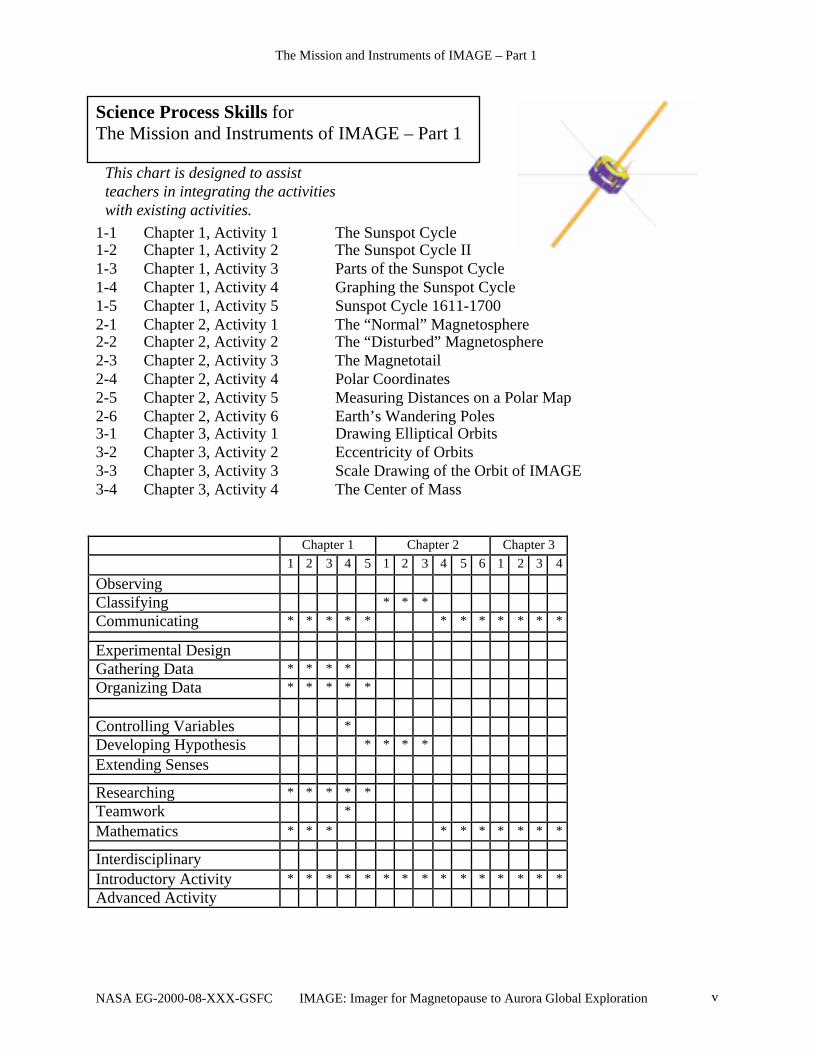
1-1 Chapter 1, Activity 1 The Sunspot Cycle1-2 Chapter 1, Activity 2 The Sunspot Cycle II1-3 Chapter 1, Activity 3 Parts of the Sunspot Cycle1-4 Chapter 1, Activity 4 Graphing the Sunspot Cycle1-5 Chapter 1, Activity 5 Sunspot Cycle 1611-17002-1 Chapter 2, Activity 1 The “Normal” Magnetosphere2-2 Chapter 2, Activity 2 The “Disturbed” Magnetosphere2-3 Chapter 2, Activity 3 The Magnetotail2-4 Chapter 2, Activity 4 Polar Coordinates2-5 Chapter 2, Activity 5 Measuring Distances on a Polar Map2-6 Chapter 2, Activity 6 Earth’s Wandering Poles3-1 Chapter 3, Activity 1 Drawing Elliptical Orbits3-2 Chapter 3, Activity 2 Eccentricity of Orbits3-3 Chapter 3, Activity 3 Scale Drawing of the Orbit of IMAGE3-4 Chapter 3, Activity 4 The Center of Mass

Chapter 1 Chapter 2 Chapter 3

1 2 3 4 5 1 2 3 4 5 6 1 2 3 4

ObservingClassifying * * *

Communicating * * * * * * * * * * * *

Experimental DesignGathering Data * * * *

Organizing Data * * * * *

Controlling Variables *

Developing Hypothesis * * * *

Extending Senses

Researching * * * * *

Teamwork *

Mathematics * * * * * * * * * *

InterdisciplinaryIntroductory Activity * * * * * * * * * * * * * * *

Advanced Activity

Science Process Skills forThe Mission and Instruments of IMAGE – Part 1

This chart is designed to assistteachers in integrating the activitieswith existing activities.

The Mission and Instruments of IMAGE – Part 1

vi NASA EG-2000-08-XXX-GSFC IMAGE: Imager for Magnetopause to Aurora Global Exploration

NATIONAL SCIENCE STANDARDS Chapter 1 Chapter 2 Chapter 3

1 2 3 4 5 1 2 3 4 5 6 1 2 3 4

A. SCIENCE AS INQUIRY Science as Inquiry * * * * * *

B. PHYSICAL SCIENCE Motions and Forces * * * * * *

Conservation of Energy Interactions of Energy and Matter * * *

C. LIFE SCIENCED. EARTH AND SPACE SCIENCE Energy in the Earth System * * *

Origin and Evolution of the Earth System * * * *

E. SCIENCE AND TECHNOLOGY Understandings about Science and Technology *

F. PERSONAL AND SOCIAL PERSPECTIVESG. HISTORY AND NATURE OF SCIENCE Science as Human Endeavor * * * * * * * * * * *

Nature of Scientific Knowledge * * * * * *

Historical Perspectives * * * * * * * * *

NCTM MATH STANDARDS Chapter 1 Chapter 2 Chapter 3

1 2 3 4 5 1 2 3 4 5 6 1 2 3 4

Number and Operations Standard Large/small numbers * * * *

Compute fluently * * * * * * *

Algebra Standard Analyze change: graphical data * *

Geometry Standard Specify locations: polar coordinates * * *

Measurement Standard Units and scales * * * * *

Data and Probability Standard Display and discuss bivariate data * *

Problem Solving Standard Apply a variety of problem solving strategies * * * *

Reasoning and Proof Standard Various types of reasoning * * *

Connection Standard Contexts outside of mathematics * * * * * * * * * * * * * * *

Science and Mathematics Standards forThe Mission and Instruments of IMAGE – Part 1

The Mission and Instruments of IMAGE – Part 1

1NASA EG-2000-08-XXX-GSFC IMAGE: Imager for Magnetopause to Aurora Global Exploration

Chapter 1

Solar Physics and the IMAGE Mission

The History of Solar Physics

For centuries, the sun has been seen as a constant in the sky. Its risings and settings aredependable; its appearance seemingly unchanging; its reliability a given in the life of humans.More recently, however, scientists have determined that the sun is surprisingly variable and thatthis variability can have very real (and detrimental) effects on Earth.

Sunspots as seen in white light.

Sunspots were an early example of variability on the sun. Sunspots are regions of the sun thatare cooler than the surrounding photosphere and therefore appear darker than the surroundingarea. More than 300 years ago, it was noticed that the number of sunspots appearing on the sunat any given time was not constant. In 1843, Heinrich Schwabe, after 17 years of carefulobservation of sunspots, noticed an 11-year cycle in the number of sunspots. The number ofsunspots seemed to increase and then decrease over time so that the highest number of sunspots(solar maximum) occurred 11 years apart with low numbers of sunspots (solar minimum)occurring in the intervening times. When scientists checked earlier sunspot observations, theyfound that the 11-year cycle had in fact been going on for over 100 years (and, presumably, formuch longer than that). As careful observations have been continued since 1843, the 11-yearcycle has been verified repeatedly. It should be noted that the sunspot cycle is not alwaysexactly 11 years, but 11 years is an average value for the length of the cycle.

The Mission and Instruments of IMAGE – Part 1

2 NASA EG-2000-08-XXX-GSFC IMAGE: Imager for Magnetopause to Aurora Global Exploration

While the cyclic variability of sunspots was interesting to scientists, there was no obviousconnection between the sunspot cycle and anything happening on Earth. In 1859, a connectionwould be observed for the first time.

While observing sunspots on September 1, 1859, Richard Carrington noticed a pronouncedbrightening of a region near the sunspots, which then faded in brightness back to that of the solarsurface. Less than a day later the aurora showed a large increase in brightness. What Carringtonhad seen was a solar flare, which is an eruption of material from the solar surface. The ensuingincrease in the aurora is called a magnetic storm. The connection between activity on the sun, asevidenced by sunspots and solar flares, and events on Earth has been investigated by scientistsever since.

A Solar Flare

The Mission and Instruments of IMAGE – Part 1

3NASA EG-2000-08-XXX-GSFC IMAGE: Imager for Magnetopause to Aurora Global Exploration

A connection between the sun and Earth that was postulated was the “solar wind”. The solarwind is a stream of charged particles, called a plasma, flowing outward from the sun in alldirections. This combination of positive ions and free electrons could not be detected directlyuntil the early years of the space age. Particle detectors on some early spacecraft measured thecomposition and speed of the solar wind particles. Since the solar wind consists of chargedparticles, the motion of these particles is affected by any magnetic fields they encounter. Thearrival of these energetic particles in the upper atmosphere of the Earth is what results in theaurora. The auroras occur near the north- and south- magnetic poles because the solar windparticles follow Earth’s magnetic field lines to those regions.

In 1973, a new phenomenon on the sun was observed from Skylab. This was a very large-scaleeruption from the sun’s upper atmosphere – the corona. Called coronal mass ejections, CMEs,these eruptions are larger than flares and produce even higher speed particles. It is thought thatCMEs have the most effect on the Earth environment of any solar activity.

A Coronal Mass Ejection (CME). The sun is represented by the dashed circle in the upper right of each frame.

The images represent a time span of 3.5 hours.

The IMAGE spacecraft is continuing the investigation of the connection between solar activitylevels and the Earth. In order to understand what the IMAGE mission will study, we must firstknow something about the Earth and its magnetic field.

The Mission and Instruments of IMAGE – Part 1

4 NASA EG-2000-08-XXX-GSFC IMAGE: Imager for Magnetopause to Aurora Global Exploration

The Sunspot Cycle - A Series of ActivitiesMaterials needed: (The following activities can be done in sequence or separate activities can be selected.)

Students: Piece of notebook paper for tables plus:Activities 1,2,3 Sunspot Number 1700 - 1996 (Table 1 Parts 1 and 2)Activity 4 Graph paperActivity 5 Sunspot Number 1611 - 1700 (Table 3)

Teacher:Activities 1,2,3 Transparency of Table 1 Part 1Activity 3 Transparency of Table 2 (Maxima and Minima ...)Activity 4 Transparency of graph paper with scales indicatedActivity 5 Transparency of Table 3;

Transparency of "Graph of Sunspot Numbers"Activity 1

Distribute a copy of the Sunspot Number Data to each student or pair of students.

Instructions for students:

1. Start at the top of any column on page 1 or the first column (1851) on page 2 of the Data Table.(Teacher: Make sure some students (or groups) start at the top of each column.)

2. Scan down the column until you find the first maximum number of sunspots. You can recognize a maximumbecause after the maximum, the number of sunspots becomes smaller. Circle the first maximum.(Teacher: use the transparency of Table 1 Part 1 to demonstrate this step. Use the column headed 1791 as yourexample. In this column, two potential difficulties are illustrated. First, the number at the top is a high number andthe following numbers become smaller. The first number in this column is NOT a maximum as can be seen bylooking at the bottom of the preceding column. In searching farther down for the first maximum, the secondproblem with the data appears. The sunspot number for 1802 (45) is followed by a smaller number the next year(43) which is then followed by a larger number in 1804 (48). 1804 is the first maximum in this column. It shouldbe pointed out that while the sunspot number changes from high to lower to high in two years, this does notrepresent more than one sunspot cycle! The sunspot numbers for 1802-03-04 should be viewed as staying fairlyconstant with the 1804 value representing the maximum. This is NOT the only place in the data where the steadyincrease followed by steady decrease is not the rule, and if you do not point out this problem with the data, theresults of the activity will not be satisfactory. A third problem that will arise is when the sunspot number is the samefor 2 (or more) years and it is a maximum value: Which year is the maximum? Here you can point out that since weare finding the average value, it does not matter much which year you choose since the average value of the adjacentcycles will not be affected. Or you can just use a rule such as "Choose the first value if there is a repeated value.")

3. Continue down the column circling each maximum as you come to it. Continue until you have circled ten moremaxima. (Total of 11 maxima circled.)

4. Count the number of years from one maximum to the next and record in a column headed

Cycle LengthMax to Max(Years)

5. Find the average number of years between maxima. This is the length of the sunspot cycle.(Teacher: Notice that students are finding the average value of 10 numbers, so calculators should be unnecessary.There will be some variation in this average, but all results should round off to 11.)

The Mission and Instruments of IMAGE – Part 1

5NASA EG-2000-08-XXX-GSFC IMAGE: Imager for Magnetopause to Aurora Global Exploration

Activity 1 (continued)

Questions to consider:

1. Is the cycle length the same each time?2. What is the longest cycle length found?3. What is the shortest cycle length found?3. Do the average cycle lengths have anything in common?4. The last sunspot maximum occurred in 1989. When would we expect the next solar maximum? Are we sure it will happen exactly then?

Activity 2

Instructions to students:

1. Using the same Data Table, starting in the same column as Activity 1, and beginning at your first circledmaximum, scan down the column and draw a box around each minimum number of sunspots.(Teacher: If colored pencils are available, different colors could be used to identify maxima and minima.)

2. Continue this until you have boxed the minimum after the last maximum circled in Activity 1. A total of 11minima will be boxed.

3. Count the number of years between sunspot minima and record in a table column headed:

Cycle LengthMin to Min(Years)

4. Find the average number of years between minima. This is another way to determine the length of the sunspotcycle.

Questions to consider:

1. Is the cycle length the same each time?2. What is the longest cycle length found?3. What is the shortest cycle length found?3. Do the average cycle lengths have anything in common?

Activity 3

1. Using the same Data Table and starting in the same column, count the number of years between the firstmaximum and the following minimum. Record this in a table headed

Fall to Minimum(Years)

2. Move to the next maximum and continue this process until the column has 10 entries.

3. Find the average number of years for the sunspot number to fall to the minimum.

4. Count the number of years between each minimum and the next maximum. Record this data in a column headed:

Rise to Maximum(Years)

The Mission and Instruments of IMAGE – Part 1

6 NASA EG-2000-08-XXX-GSFC IMAGE: Imager for Magnetopause to Aurora Global Exploration

Activity 3 (continued)

5. Move to the next minimum and continue this process until the column has 10 entries.

6. Find the average number of years for the sunspot number to rise to maximum.

Questions:

1. What is the range of values in the "Fall to Minimum" column?2. What is the average value for the "Fall to Minimum"?3. What is the range of values in the "Rise to Maximum" column?4. What is the average value for the "Rise to Maximum"?5. Are the rise times and fall times the same?

(Teacher: Rise times average 4.8 years, Fall times average 6.2 years. It is important that students see these times asdifferent. Display a transparency of the Table 2 "MINIMA AND MAXIMA ..." .)

Activity 4

1. Use the graph paper provided (Page 13). Notice that the highest sunspot number available on the graph paper is120. If a higher sunspot number is encountered in the data, the point can be positioned above the grid with the valuewritten next to the point.

2. Plot the yearly sunspot number for each year in the range you have been assigned. Be sure to label the years onthe horizontal axis.(Teacher: Each student can be assigned a range of years starting from a given year. Ranges for each student can be30 years, 50 years, or 100 years.)

3. Connect the points on your graph.

4. Get together with other students who have used different years and tape the graphs together on the front board.

Questions to consider:

1. Is the Solar Cycle easy to see when looking at the graph?2. Is the spacing between the maxima exactly constant on the graph? Did you expect it to be?3. Is it true to say that the Solar Cycle is exactly 11 years long?

Activity 5

(Teacher: Distribute a copy of Table 3 Sunspot Number 1611 - 1700 to each group.)

Questions:

1. What is the most common sunspot number that appears on this table?2. During how many years (of the 90 years shown) is the sunspot number zero?3. The sunspot number is missing for how many years?4. Why do you suppose the numbers are missing for these years?

(Teacher: Display a transparency of the sunspot graph.)

5. What is the period from about 1640 to 1700 called? Why is it called this?

The Mission and Instruments of IMAGE – Part 1

7NASA EG-2000-08-XXX-GSFC IMAGE: Imager for Magnetopause to Aurora Global Exploration

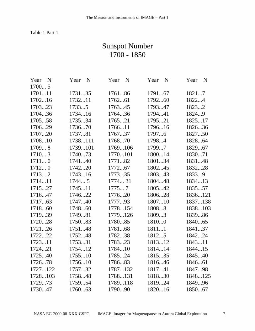
Table 1 Part 1

Sunspot Number1700 - 1850

Year N Year N Year N Year N Year N1700... 51701...11 1731...35 1761...86 1791...67 1821...71702...16 1732...11 1762...61 1792...60 1822...41703...23 1733...5 1763...45 1793...47 1823...21704...36 1734...16 1764...36 1794...41 1824...91705...58 1735...34 1765...21 1795...21 1825...171706...29 1736...70 1766...11 1796...16 1826...361707...20 1737...81 1767...37 1797...6 1827...501708...10 1738...111 1768...70 1798...4 1828...641709... 8 1739...101 1769...106 1799...7 1829...671710... 3 1740...73 1770...101 1800...14 1830...711711... 0 1741...40 1771...82 1801...34 1831...481712... 0 1742...20 1772...67 1802...45 1832...281713... 2 1743...16 1773...35 1803...43 1833...91714...11 1744... 5 1774... 31 1804...48 1834...131715...27 1745...11 1775... 7 1805...42 1835...571716...47 1746...22 1776...20 1806...28 1836...1211717...63 1747...40 1777...93 1807...10 1837...1381718...60 1748...60 1778...154 1808...8 1838...1031719...39 1749...81 1779...126 1809...3 1839...861720...28 1750...83 1780...85 1810...0 1840...651721...26 1751...48 1781...68 1811...1 1841...371722...22 1752...48 1782...38 1812...5 1842...241723...11 1753...31 1783...23 1813...12 1843...111724...21 1754...12 1784...10 1814...14 1844...151725...40 1755...10 1785...24 1815...35 1845...401726...78 1756...10 1786...83 1816...46 1846...611727...122 1757...32 1787...132 1817...41 1847...981728...103 1758...48 1788...131 1818...30 1848...1251729...73 1759...54 1789...118 1819...24 1849...961730...47 1760...63 1790...90 1820...16 1850...67

The Mission and Instruments of IMAGE – Part 1

8 NASA EG-2000-08-XXX-GSFC IMAGE: Imager for Magnetopause to Aurora Global Exploration

Table 1 Part 2

Sunspot Number1851 - 1996

Year N Year N Year N Year N Year N1851...64 1881...54 1911...6 1941...47 1971...671852...54 1882...60 1912...4 1942...31 1972...691853...39 1883...64 1913...1 1943...16 1973...381854...20 1884...64 1914...10 1944...10 1974...341855...7 1885...52 1915...47 1945...33 1975...161856...4 1886...25 1916...57 1946...93 1976...131857...22 1887...13 1917...104 1947...152 1977...271858...59 1888...7 1918...81 1948...136 1978...921859...94 1889...6 1919...64 1949...135 1979...1551860...96 1890...7 1920...38 1950...84 1980...1541861...77 1891...36 1921...26 1951...69 1981...1401862...59 1892...73 1922...14 1952...31 1982...1161863...44 1893...85 1923...6 1953...14 1983...671864...47 1894...78 1924...17 1954...4 1984...461865...31 1895...64 1925...44 1955...38 1985...181866...16 1896...42 1926...64 1956...142 1986...141867...7 1897...26 1927...69 1957...190 1987...321868...38 1898...27 1928...78 1958...185 1988...981869...74 1899...12 1929...65 1959...159 1989...1541870...139 1900...9 1930...36 1960...112 1990...1461871...111 1901...3 1931...21 1961...54 1991...1441872...102 1902...5 1932...11 1962...38 1992...941873...66 1903...24 1933...6 1963...28 1993...561874...45 1904...42 1934...9 1964...10 1994...301875...17 1905...63 1935...36 1965...15 1995...171876...11 1906...54 1936...80 1966...47 1996...91877...12 1907...62 1937...114 1967...941878... 3 1908...48 1938...110 1968...1061879... 6 1909...44 1939...89 1969...1061880...32 1910...19 1940...68 1970...104

www.ngdc.noaa.gov/stp/stp.html

The Mission and Instruments of IMAGE – Part 1

9NASA EG-2000-08-XXX-GSFC IMAGE: Imager for Magnetopause to Aurora Global Exploration

MINIMA AND MAXIMA OF SUNSPOT NUMBER CYCLES==================================================================Sunspot Year Smallest Year Largest Rise Fall Cycle Cycle of Smoothed of Smoothed to to Length Number Min* Monthly Max* Monthly Max Min

Mean** Mean** (Yrs) (Yrs) (Yrs)------------------------------------------------------------------------------- - 1610.8 -- 1615.5 -- 4.7 3.5 8.2 - 1619.0 -- 1626.0 -- 7.0 8.0 15.0 - 1634.0 -- 1639.5 -- 5.5 5.5 11.0 - 1645.0 -- 1649.0 -- 4.0 6.0 10.0 - 1655.0 -- 1660.0 -- 5.0 6.0 11.0 - 1666.0 -- 1675.0 -- 9.0 4.5 13.5 - 1679.5 -- 1685.0 -- 5.5 4.5 10.0 - 1689.5 -- 1693.0 -- 3.5 5.0 8.5 - 1698.0 -- 1705.5 -- 7.5 6.5 14.0 - 1712.0 -- 1718.2 -- 6.2 5.3 11.5 - 1723.5 -- 1727.5 -- 4.0 6.5 10.5 - 1734.0 -- 1738.7 -- 4.7 6.3 11.0 - 1745.0 -- 1750.3 92.6 5.3 4.9 10.2 1 1755.2 8.4 1761.5 86.5 6.3 5.0 11.3 2 1766.5 11.2 1769.7 115.8 3.2 5.8 9.0 3 1775.5 7.2 1778.4 158.5 2.9 6.3 9.2 4 1784.7 9.5 1788.1 141.2 3.4 10.2 13.6 5 1798.3 3.2 1805.2 49.2 6.9 5.4 12.3 6 1810.6 0.0 1816.4 48.7 5.8 6.9 12.7 7 1823.3 0.1 1829.9 71.7 6.6 4.0 10.6 8 1833.9 7.3 1837.2 146.9 3.3 6.3 9.6 9 1843.5 10.5 1848.1 131.6 4.6 7.9 12.5 10 1856.0 3.2 1860.1 97.9 4.1 7.1 11.2 11 1867.2 5.2 1870.6 140.5 3.4 8.3 11.7 12 1878.9 2.2 1883.9 74.6 5.0 5.7 10.7

The Mission and Instruments of IMAGE – Part 1

10 NASA EG-2000-08-XXX-GSFC IMAGE: Imager for Magnetopause to Aurora Global Exploration

MINIMA AND MAXIMA OF SUNSPOT NUMBER CYCLES==================================================================Sunspot Year Smallest Year Largest Rise Fall Cycle Cycle of Smoothed of Smoothed to Max to Min Length Number Min* Monthly Max* Monthly (Yrs) (Yrs) (Yrs)

Mean** Mean** 13 1889.6 5.0 1894.1 87.9 4.5 7.6 12.1 14 1901.7 2.6 1907.0 64.2 5.3 6.6 11.9 15 1913.6 1.5 1917.6 105.4 4.0 6.0 10.0 16 1923.6 5.6 1928.4 78.1 4.8 5.4 10.2 17 1933.8 3.4 1937.4 119.2 3.6 6.8 10.4 18 1944.2 7.7 1947.5 151.8 3.3 6.8 10.1 19 1954.3 3.4 1957.9 201.3 3.6 7.0 10.6 20 1964.9 9.6 1968.9 110.6 4.0 7.6 11.6 21 1976.5 12.2 1979.9 164.5 3.4 6.9 10.3 22 1986.8 12.3 1989.6 158.5 2.8-------------------------------------------------------------------------------Mean Cycle Values: 6.0 112.9 4.8 6.2 11.1------------------------------------------------------------------------------- *When observations permit, a date selected as either a cycle minimum or maxi- mum is based in part on an average of the times extremes are reached in the monthly mean sunspot number, in the smoothed monthly mean sunspot number, and in the monthly mean number of spot groups alone. Two more measures are used at time of sunspot minimum: the number of spotless days and the frequency of occurrence of "old" and "new" cycle spot groups.

**The smoothed monthly mean sunspot number is defined here as the arithmetic average of two sequential 12-month running means of monthly mean numbers.

ftp://ftp.ngdc.noaa.gov/STP/SOLAR_DATA/SUNSPOT_NUMBERS/maxmin

The Mission and Instruments of IMAGE – Part 1

11NASA EG-2000-08-XXX-GSFC IMAGE: Imager for Magnetopause to Aurora Global Exploration

Table 3

Sunspot Number1611 - 1700

Year N Year N Year N

1611 30 1641 1671 61612 53 1642 6 1672 41613 28 1643 16 1673 01614 1644 15 1674 21615 1645 0 1675 01616 1646 1676 101617 1647 1677 21618 1648 1678 61619 1649 1679 01620 1650 0 1680 41621 1651 0 1681 21622 1652 3 1682 01623 1653 0 1683 01624 1654 2 1684 111625 41 1655 1 1685 01626 40 1656 2 1686 41627 22 1657 0 1687 01628 1658 0 1688 51629 1659 0 1689 41630 1660 4 1690 01631 1661 4 1691 01632 1663 0 1692 01633 1663 0 1693 01634 1664 0 1694 01635 1665 0 1695 01636 1666 0 1696 01637 1667 0 1697 01638 1668 0 1698 01639 1669 0 1699 01640 1670 0 1700 2

NOTE: Sunspot numbers were not determined in the same way for this table as for the previoustable. The actual sunspot number, when it is greater than zero, during this time would probablyhave been higher if the same rule for determining sunspot number had been used. When thesunspot number is zero, it would probably be that regardless of the rule used for calculating it.

ftp://ftp.ngdc.noaa.gov/STP/SOLAR_DATA/SUNSPOT_NUMBERS/

The Mission and Instruments of IMAGE – Part 1

12 NASA EG-2000-08-XXX-GSFC IMAGE: Imager for Magnetopause to Aurora Global Exploration

Graph of Sunspot Numbers

1600 1620 1640 1660 1680 1700 1720 1740

1740 1760 1780 1800 1820 1840 1860

1860 1880 1900 1920 1940 1960 1980 2000

The Mission and Instruments of IMAGE – Part 1

13NASA EG-2000-08-XXX-GSFC IMAGE: Imager for Magnetopause to Aurora Global Exploration

120

110

100

90

80

70

60

50

40

30

20

10

0

__0

0

1

0

20

3

0

40

__5

0

6

0

70

80

9

0

__

00

SUN

SPO

TS

Sunspot Number

Yea

r

The Mission and Instruments of IMAGE – Part 1

14 NASA EG-2000-08-XXX-GSFC IMAGE: Imager for Magnetopause to Aurora Global Exploration

Chapter 2

Earth’s Magnetosphere and the IMAGE Mission

For hundreds of years, sailors have relied on magnetic compasses to navigate the oceans. Thesesailors knew that the Earth’s magnetic north pole was not in the same place as the geographicNorth Pole, and they were able to make the necessary corrections to be able to determine wherethey were (and, more important, how to get home!). In modern times, we have found that themagnetic north pole does not even stay in the same place, but moves around a significantamount. Small corrections are needed in order to use the magnetic pole for navigation purposes.

Figure 1. The Magnetic Field of a bar magnet.Notice the symmetry and direction of the field lines.Remember, the magnetic north pole is not located

in the same place as the geographic North Pole

The Earth has a magnetic field that has a shape similar to that of a large bar magnet (Figure 1).To the north is the magnetic north pole, which is really the south pole of the Earth’s bar magnet.(It has to be this way since this pole attracts the north pole of the compass magnet!) The sun alsohas a magnetic field that is more complicated than, but similar to, that of the Earth. The sun,through its solar wind, has a large impact on the shape of Earth’s magnetic field.

As the solar wind flows outward from the sun and encounters Earth’s magnetic field, it pushesthe Earth’s field in on the side toward the sun and stretches it out on the side away from the sun.The result is a magnetic field shape that is not symmetric in the same way as the field of a barmagnet. The region around Earth where Earth’s magnetic field is the predominate field is calledthe magnetosphere (Figure 2). Outside this region, in the region called the InterplanetaryMagnetic Field (IMF), the solar magnetic field is strongest. The boundary line between themagnetosphere and the IMF is called the magnetopause. The part of the magnetosphere thatextends from Earth away from the sun is called the magnetotail.

S

N

The Mission and Instruments of IMAGE – Part 1

15NASA EG-2000-08-XXX-GSFC IMAGE: Imager for Magnetopause to Aurora Global Exploration

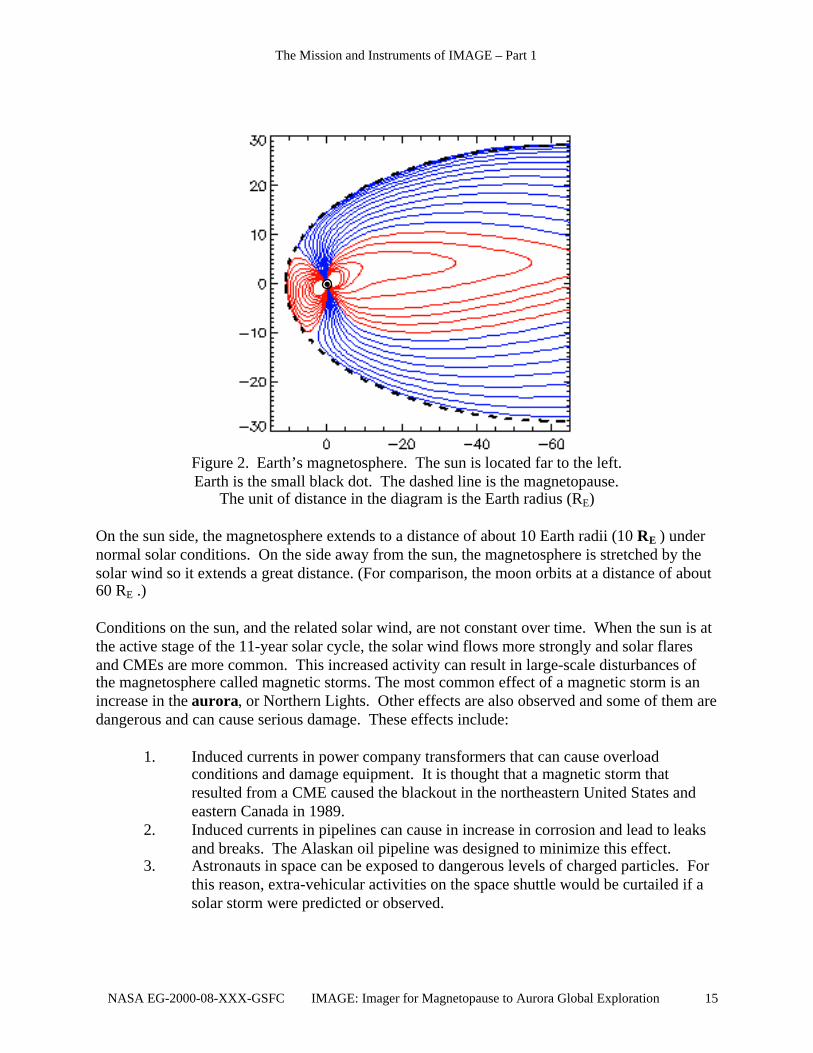
Figure 2. Earth’s magnetosphere. The sun is located far to the left.Earth is the small black dot. The dashed line is the magnetopause.

The unit of distance in the diagram is the Earth radius (RE)

On the sun side, the magnetosphere extends to a distance of about 10 Earth radii (10 RE ) undernormal solar conditions. On the side away from the sun, the magnetosphere is stretched by thesolar wind so it extends a great distance. (For comparison, the moon orbits at a distance of about60 RE .)

Conditions on the sun, and the related solar wind, are not constant over time. When the sun is atthe active stage of the 11-year solar cycle, the solar wind flows more strongly and solar flaresand CMEs are more common. This increased activity can result in large-scale disturbances ofthe magnetosphere called magnetic storms. The most common effect of a magnetic storm is anincrease in the aurora, or Northern Lights. Other effects are also observed and some of them aredangerous and can cause serious damage. These effects include:

1. Induced currents in power company transformers that can cause overloadconditions and damage equipment. It is thought that a magnetic storm thatresulted from a CME caused the blackout in the northeastern United States andeastern Canada in 1989.

2. Induced currents in pipelines can cause in increase in corrosion and lead to leaksand breaks. The Alaskan oil pipeline was designed to minimize this effect.

3. Astronauts in space can be exposed to dangerous levels of charged particles. Forthis reason, extra-vehicular activities on the space shuttle would be curtailed if asolar storm were predicted or observed.

The Mission and Instruments of IMAGE – Part 1

16 NASA EG-2000-08-XXX-GSFC IMAGE: Imager for Magnetopause to Aurora Global Exploration

4. Heating of the atmosphere by solar particles causes the atmosphere to expandslowing low orbit satellites and causing them to descend. This is the process thatis thought to have caused the decay of the orbit of Skylab in the 1970’s.

5. Satellites in high orbits are subjected to energetic charged particles that can causedamage to electronic components. Failure of some communication satellites,which are in geosynchronous orbits, has been attributed to magnetic storms.

6. Radio communications can be disrupted because of changes in the region nearEarth.

Figure 3. The magnetosphere under quiet solar conditions.The dashed line is the magnetopause.

The two main effects on the magnetosphere of magnetic storms are:

1. The magnetopause in the sunward direction is pushed in from its normal distance of10 RE .

2. The magnetotail is pinched inward.

The added pressure on the sunward side increases the number of particles that are forced into themagnetosphere where they follow magnetic field lines north and south into the lower atmospherein the polar regions. This causes the brightening of the aurora.

In the magnetotail, charged particles are following the magnetic field lines down the tail awayfrom Earth. When the magnetotail gets pinched in, a phenomenon called magneticreconnection can occur. This happens when magnetic field lines within the magnetotail areforced together in such a way that they try to cross (which is not allowed for magnetic field lines)and, instead, reconnect forming a shorter, closed magnetic field line in place of the extremely

10 RE

Geosynchronous satellite orbit at adistance of 6.6 RE from the center of Earth

The Mission and Instruments of IMAGE – Part 1

17NASA EG-2000-08-XXX-GSFC IMAGE: Imager for Magnetopause to Aurora Global Exploration

long field lines extending down the magnetotail. Figures 4, 5 and 6 show the reconnectionprocess.

Figure 4. The magnetosphere under active solar conditions after a CME.The sunward magnetopause has been pushed in to 6 RE and

the magnetotail has been pinched in (arrows).Note that the geosynchronous orbit now extends outside of the magnetopause.

Figure 5. The arrows indicate the point of magnetic reconnection.

6 RE

6 RE

The Mission and Instruments of IMAGE – Part 1

18 NASA EG-2000-08-XXX-GSFC IMAGE: Imager for Magnetopause to Aurora Global Exploration

Figure 6. The magnetic field lines just after reconnection.The arrows indicate the direction of movement of the magnetic field lines

which carry with them all of the charged particles movingalong them at the time of reconnection.

The process of reconnection results in large numbers of particles moving with high energy bothtoward and away from Earth. It is thought that the process that carries particles away from Earthis similar to, but on a smaller scale than, the process on the sun that results in a CME. Of interesthere, though, are the particles that are brought back toward Earth as the reconnected field linerebounds into position nearer Earth. Some of these charged particles find an easy path north andsouth into the auroral zones and some of them are captured near the Earth and held there bymagnetic field lines forming the radiation belts. As these particles move along magnetic fieldlines north and south, they rebound back along the field line from the polar regions. As theybounce back and forth, the charges migrate slowly around the Earth in the region from about 2RE to about 7 RE. This movement of charge is known as the ring current.

IMAGE will measure the location of the magnetopause, the brightness and location of the auroraand the composition, energy and location of the ring current.

6 RE

The Mission and Instruments of IMAGE – Part 1

19NASA EG-2000-08-XXX-GSFC IMAGE: Imager for Magnetopause to Aurora Global Exploration

The Magnetosphere

Using the templates:

7. Make copies of the three templates on heavy paper or card stock (1 set perstudent).

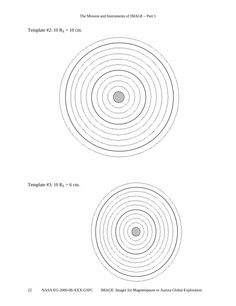
8. On each template, the center (gray) circle represents the Earth. Concentric circlesare each 1 Earth Radius (1 RE) larger in radius than the preceding circle.

9. To use the template, place it under the paper so that the circles can be seenthrough the paper. The circles at radius equals 5 RE and 10 RE from the center ofthe Earth are solid lines to make them easier to see.

Activity 1. The size and shape of “normal” magnetosphere

3. Use Template #1 and orient the paper with the long dimension vertical.4. At the far left of the page label the “SUN” and indicate with arrows the direction of

the light from the sun and the solar wind – from left to right.5. Move the template so that the Earth is centered between the top and bottom of the

page and about 10 centimeters from the left edge of the page.6. Trace the Earth from the center of the template and shade it in.7. Directly to the left of the Earth (toward the sun) place a mark at 10 RE.8. Directly above and below the Earth, place marks at 15 RE. Notice that the template

only goes to 11 RE, so you will have to estimate this location.9. Draw a smooth shape connecting the first mark with the top mark and extend the

shape off the page to the right. Do the same with the first mark and the bottom mark.10. Label this shape: “Magnetopause”

Under normal conditions of solar wind, the magnetopause is located at about 10 RE from theEarth towards the sun. The magnetotail extends a large distance (many 10s of RE) in thedirection away from the sun.

Activity 2. The “disturbed” magnetosphere

1. Use Template #2 and orient the paper with the long dimension vertical.2. At the far left of the page label the “SUN” and indicate with arrows the direction of the

light from the sun and the solar wind – from left to right.3. For this activity, two diagrams will be drawn on the page. The first will be on the top

half of the page; the second will be on the bottom half.4. On the top half, place the template with the Earth about 6 centimeters from the left edge

of the page. Draw the “normal” magnetosphere as in Activity 1. Label this diagram“Normal Magnetosphere”.

5. On the bottom half, place the template so that the Earth lines up directly under the firstdiagram. From the Earth, count out 7 RE to the left and place a mark.

6. Directly above and below, place marks at 10 RE.7. Draw a smooth shape to represent the magnetopause. Label this diagram “Disturbed

Magnetosphere”

The Mission and Instruments of IMAGE – Part 1

20 NASA EG-2000-08-XXX-GSFC IMAGE: Imager for Magnetopause to Aurora Global Exploration

“Disturbed” conditions occur with the arrival of the increased solar wind levels as the result of acoronal mass ejection (CME). The effect of this magnetic storm is to push the magnetopause intoward the Earth from the sunward direction (from 10 RE to 7 RE or even less). Themagnetosphere is also compressed inward toward Earth above and below and the magnetotail isalso constricted.

Activity 3. The magnetotail

1. Use Template #2 and orient the paper with the long dimension horizontal.2. At the far left of the page label the “SUN” and indicate with arrows the direction of the

light from the sun and the solar wind – from left to right.3. For this activity, two diagrams will be drawn on the page. The first will be on the top

half of the page; the second will be on the bottom half.4. On the top half, place the template with the Earth about 6 centimeters from the left edge

of the page. Locate the sunward magnetopause (10 RE) and the positions above andbelow Earth (15 RE) as in Activity 1. When you draw in the magnetopause and extendthe shape to the right, allow the lines to extend all the way across the page without gettingvery close together. This is the magnetotail. The magnetotail extends in the directionaway from the sun for a very large distance (tens of RE).

5. On the bottom half, place the template so that the Earth lines up directly under the firstdiagram. From the Earth, count out 7 RE to the left and place a mark. Above and belowthe Earth, place marks at 10 RE. Draw in the magnetopause, but when you extend themagnetopause to the right draw the shape so that there is a pronounced narrowing of themagnetotail as the magnetopause boundaries extend off the page.

It is in this area of constriction of the magnetotail that reconnection occurs under solar stormconditions. When reconnection occurs, particles that are following magnetic field lines in thetailward direction can be rerouted back toward Earth. These particles, which under normalconditions would be lost into the magnetotail, return toward Earth where they contribute to theaurora and provide charged particles for the ring current and other structures in theplasmasphere. The IMAGE satellite will attempt to determine the exact paths and timing of themovement of these charges in magnetic storm conditions.

The Mission and Instruments of IMAGE – Part 1

21NASA EG-2000-08-XXX-GSFC IMAGE: Imager for Magnetopause to Aurora Global Exploration

Template #1: 10 RE = 15 cm.

The Mission and Instruments of IMAGE – Part 1

22 NASA EG-2000-08-XXX-GSFC IMAGE: Imager for Magnetopause to Aurora Global Exploration

Template #2: 10 RE = 10 cm.

Template #3: 10 RE = 6 cm.

The Mission and Instruments of IMAGE – Part 1

23NASA EG-2000-08-XXX-GSFC IMAGE: Imager for Magnetopause to Aurora Global Exploration

TEACHER NOTES

The Wandering Magnetic Pole

The purpose of the activities:

To investigate the nature of the magnetic North Pole, a position that is often thought of asconstant but, in fact, moves significantly over the years.

Objective:

To develop perceptual abilities using polar coordinates, a frame of reference new to manystudents.

Procedure:

6. Make transparencies of any desired materials from the student activity pages.7. Copy and distribute the student activity pages.8. Introduce the material in a manner suited to the class level:0 Ninth grade students may need some introduction to some (or each) separate activity.1 Twelfth grade students should be able to work all activities with no intervention by

the teacher.9. Go over some (or all) of the responses using a transparency key done by the

teacher. Discuss the precision available in the data and maps in light of the variations inresponses from students that may be considered equivalent. (For example, estimates ofprecision are given for each activity here:

Activity 4: Latitude: ± .2o Longitude: ± 5 o

Activity 5: Distance: ± 10 kilometersActivity 6: Location of pole is a function of the precision of each of the three

quantities listed above. If the pole position is in the correct grid space,that is probably good enough.

Extension and homework assignments:

Blank map grids are provided for the teacher to create custom assignments similar toactivities 4 and 5.

Activity 6 can be used as a homework assignment by selecting a different pair of dates(for example 1500 – 1600) and having the students answer questions 1 to 4 from Activity 6.

The Mission and Instruments of IMAGE – Part 1

24 NASA EG-2000-08-XXX-GSFC IMAGE: Imager for Magnetopause to Aurora Global Exploration

Shown below is a view of the Earth with the geographic North Pole at the center.

Latitude is shown as concentric circles with the North Pole having a latitude of 90o. Notice thatthis map shows only the region very near the North Pole. Longitude is measured in degreesmeasured from the Prime Meridian (0o) which passes through Greenwich, England. Longitudecan be given in degrees east or west of the Prime Meridian or in degrees measuredcounterclockwise from the Prime Meridian. In these activities we will use degrees measured

counterclockwise from the Prime Meridian, so longitude can have a value of from 0o to 360o.

(Blank map grid.)

0 500 kilometers

West East0o

30o

60o

120o E

150o E

60o E

30o E

180o

180o

150o

120o

90o

30o W

60o W

90o W

120o W

150o W

210o

240o

270o

300o

330o

90o

88o

86o

84o

82o

80o

The Mission and Instruments of IMAGE – Part 1

25NASA EG-2000-08-XXX-GSFC IMAGE: Imager for Magnetopause to Aurora Global Exploration

Activity 4. Plotting Positions in Polar Coordinates

Using the map shown, give the positions of the lettered locations. The first answer isgiven. Notice that you have estimate latitude values since the concentric circles represent 2degree increments. Longitude values must also be estimated since the longitude lines shown are30 degrees apart. (Because of the estimating required, you should only expect your answer to bewithin a degree of the given answer for latitude and within about 5 degrees for longitude.)

Point Latitude Longitude

A 82.7o 167o

B

C

D

E

West East0o

30o

60o

120o E

150o E

60o E

30o E

180o

180o

150o

120o

90o

30o W

60o W

90o W

120o W

150o W

210o

240o

270o

300o

330o

90o

88o

86o

84o

82o

80o

A •

B •

D •

C •

E •

The Mission and Instruments of IMAGE – Part 1

26 NASA EG-2000-08-XXX-GSFC IMAGE: Imager for Magnetopause to Aurora Global Exploration

On the map shown below, plot the points given. Remember to estimate between the latitudecircles and the longitude lines. Watch the labels carefully as you find the correct positions. Thefirst example is shown on the map.

Point Latitude Longitude

A 88o 310o

B 82o 60o

C 85o 195o

D 81.7o 260o

E 83.9o 121o

West East0o

30o

60o

120o E

150o E

60o E

30o E

180o

180o

150o

120o

90o

30o W

60o W

90o W

120o W

150o W

210o

240o

270o

300o

330o

90o

88o

86o

84o

82o

80o

The Mission and Instruments of IMAGE – Part 1

27NASA EG-2000-08-XXX-GSFC IMAGE: Imager for Magnetopause to Aurora Global Exploration

Activity 5. Measuring Distance on the Polar Map

Using the distance scale given, make a scale on a separate paper that will allow you tomeasure distances up to 2000 kilometers. Using the map below, measure the distances indicatedin the table. The first example is worked for you.

From Point To Point distance

A B 1400 km

B C

C D

D E

E A

B D

C A

E B

West East0o

30o

60o

120o E

150o E

60o E

30o E

180o

180o

150o

120o

90o

30o W

60o W

90o W

120o W

150o W

210o

240o

270o

300o

330o

90o

88o

86o

84o

82o

80o

A •

B •

D •

C •

E •

0 500 kilometers

The Mission and Instruments of IMAGE – Part 1

28 NASA EG-2000-08-XXX-GSFC IMAGE: Imager for Magnetopause to Aurora Global Exploration

Activity 6. Earth's Wandering Poles

Before igneous rocks cool and harden, the liquid magma is acted on by the magnetic fieldof Earth. This causes the iron atoms in the rock to align with the magnetic field and "point"toward the magnetic north pole of Earth. When the rock hardens, these iron atoms are locked inposition "pointing" toward the magnetic north pole. When scientists analyzed rocks formed atdifferent times in the past, they found that the magnetic pointers did not point to the samelocation of earth. They interpreted this to mean that the position of the magnetic North Pole hadmoved over time. The magnetic North Pole is still moving today and, using modern instruments,we can measure this movement from year to year.

The following table shows the estimated position of the North Geomagnetic Pole over thepast 2000 years. (This table is taken from The Earth's Magnetic Field by Ronald Merrill andMichael McElhinny, published in 1983 by Academic Press, page 100.) Plot the followingpositions on the map provided.

Year (AD) Latitude Longitude

0 86.4 121.4 100 87.7 143.9

200 87.7 160.3 300 88.9 131.9 400 86.0 316.3 500 86.1 343.5 600 85.6 6.6 700 84.1 33.4

800 81.8 28.0 900 80.2 38.0

1000 81.3 76.01100 85.3 110.01200 84.3 135.21300 83.2 189.11400 84.8 228.31500 86.3 301.51600 85.6 316.71700 81.1 307.11800 81.1 297.11900 82.3 288.21980 82.1 284.1

The Mission and Instruments of IMAGE – Part 1

29NASA EG-2000-08-XXX-GSFC IMAGE: Imager for Magnetopause to Aurora Global Exploration

Look at the locations of the pole at 1000 AD and 1100 AD.

1. How far did the pole move? ________

2. How far did the pole move (in km) in one year? ________

3. How far did the pole move in meters in one year? ________

4. Approximately how far did the pole move per day? ________

10. Estimate when the Geomagnetic North Pole was at the ________same location as the Geographic North Pole (Latitude = 90 o).

11. What assumptions must be made to answer Question 5?

_____________________________________________________________________

West East0o

30o

60o

120o E

150o E

60o E

30o E

180o

180o

150o

120o

90o

30o W

60o W

90o W

120o W

150o W

210o

240o

270o

300o

330o

90o

88o

86o

84o

82o

80o

0 500 kilometers

The Mission and Instruments of IMAGE – Part 1

30 NASA EG-2000-08-XXX-GSFC IMAGE: Imager for Magnetopause to Aurora Global Exploration

Chapter 3

The Orbit of IMAGEKepler’s First Law of Planetary Motion

The definition of an orbit is the path followed by an object as it moves around another under theinfluence of gravity. About 400 years ago, Johannes Kepler discovered that the orbits of theplanets around the sun were in the shape of ellipses. An ellipse is the set of points such that thesum of the distances to two fixed points is constant. Each fixed point is called a focus of theellipse and the two points are called foci.

While Kepler’s First Law describes the orbit of planets around the sun, it turns out that this lawapplies to any object in orbit around any other. The simplest orbital path is a circle. This is aspecial case of Kepler’s law that occurs when the two foci are placed at the same point – thecenter of the circle. The Space Shuttle is often placed in a circular orbit around Earth. A typicalaltitude for the Space Shuttle is 400 kilometers measured from Earth’s surface. The radius oforbit for the space shuttle is equal to the radius of Earth (RE) plus the altitude:

R = RE + 400 km. (RE = 6400 kilometers.

R = 6400 + 400

R = 6800 kilometers.

Figure 1. The space shuttle orbit at an altitude of 400 kilometers.

Figure 1 shows the orbit of the Space Shuttle drawn to scale with the Earth. Notice how close toEarth the shuttle seems to be even though at this altitude it is moving well above most of theatmosphere.

Kepler’s First Law of Planetary Motion:

The planet orbits are ellipses with the sun located at one focus.

The Mission and Instruments of IMAGE – Part 1

31NASA EG-2000-08-XXX-GSFC IMAGE: Imager for Magnetopause to Aurora Global Exploration

In the case of an elliptical orbit, the distances from the object to the foci must have a constantsum. Figure 2 shows several points on an ellipse and the distances associated with them.

Figure 2. Distance: AX + XB = AY + YB = AZ + ZB

Figure 3. Parts of an elliptical orbit.

Figure 3 shows an elliptical orbit around Earth. The perigee is the point in the orbit (measuredfrom the center of Earth) where the object is closest to Earth; apogee is the point where theobject is farthest from Earth. As an object moves from apogee, it is accelerated by gravity to ahigher speed so that the speed of the object is highest at perigee. As inertia carries the objectaway from perigee, the force of gravity acts to slow the object so that it is moving at its slowestspeed when it reaches apogee. This lead to Kepler’s Second Law of Planetary Motion.

Focus A Focus B

X

Z Y

perigee apogee

EARTH

The Mission and Instruments of IMAGE – Part 1

32 NASA EG-2000-08-XXX-GSFC IMAGE: Imager for Magnetopause to Aurora Global Exploration

Kepler’s Second Law of Planetary Motion

Figure 4. Illustration of Kepler’s Second LawIf the time between t1 and t2 is the same as that between t3 and t4

then Area 1 = Area 2.When the distances between these pairs of points are compared,

the difference in speeds is apparent.

Eccentricity of Orbits

Not all ellipses look alike. Some are nearly circular and some are very stretched out and thin.Ellipses of different shapes have different eccentricities.

Figure 5. Ellipses of different eccentricities.

EARTH

Area 1 Area 2

t1

t2

t3

t4

Kepler’s Second Law of Planetary Motion:

The line connecting the planet to the sun sweeps out equal areas in equal times.

The Mission and Instruments of IMAGE – Part 1

33NASA EG-2000-08-XXX-GSFC IMAGE: Imager for Magnetopause to Aurora Global Exploration

The eccentricity of an ellipse is defined using the following diagram:

Figure 6. An ellipse with important points labeled. E : the object being orbited (Earth) F : the other focus of the ellipse P : the perigee point of the orbit A : the apogee point of the orbit

Using the points identified in Figure 6, the eccentricity (e) of an ellipse is defined by:

The Orbit of IMAGE

The orbit of the IMAGE spacecraft is described as follows:

perigee : 1000 kilometers altitudeapogee : 7 Earth radii (RE) altitude

Notice that these values are not measured from the center of Earth. Kepler’s First Law requiresthe distances to be expressed from the center of the objects. To find the distance from the centerof the Earth, you must add the radius of the Earth (approximately 6400 kilometers) to each valuefrom above:

perigee : 6400 km + 1000 km = 7400 kmapogee : 6400 km + 7(6400) km = 51,200 km (8 RE )

The eccentricity of the IMAGE orbit can be calculated from these numbers:

EF = apogee – perigee = 51,200 – 6400 = 44,800 kmPA = apogee + perigee = 51,200 + 6400 = 57,600 km

P .E

A.F

e =EF

PA

The Mission and Instruments of IMAGE – Part 1

34 NASA EG-2000-08-XXX-GSFC IMAGE: Imager for Magnetopause to Aurora Global Exploration

This is a very eccentric orbit.

The following diagram is an approximate view of the orbit of IMAGE. A more careful drawingmay be done as an activity (Activity 3).

Figure 7. The orbit of IMAGEE : the position of Earth at one focus

When earth is added in approximately to scale, we get the best view of the orbit of IMAGE.

Figure 8. The orbit of IMAGE

e =EF

PA

44,800

57,600= = .78

E

E

The Mission and Instruments of IMAGE – Part 1

35NASA EG-2000-08-XXX-GSFC IMAGE: Imager for Magnetopause to Aurora Global Exploration

The Center of Mass of Orbiting Systems

While we often think of one object orbiting another, in fact each object exerts a gravitationalforce on the other. The result is that both objects move around a common point locatedsomewhere between the centers of the objects called the center of mass. Since the center of massis essentially the “balance point” of the two-object system, its location can be determined usingthe lever equation:

m1d1 = m2d2

where: m = mass of the objectd = distance from the center of the object to the center of mass of the system1 : object 12 : object 2

Sometimes it is acceptable to think of one object orbiting another, but sometimes it is veryimportant to include the effects of each on the other and talk about their motions about the centerof mass of the system.

When two objects have nearly the same mass, their center of mass is located about halfwaybeteen them. In that case, the two objects would be seen as orbiting each other. Some binarystars have nearly the same mass and this would be their type of apparent motion.

When one object is significantly larger than the other, the two objects would orbit a point that iscloser to the more massive object. In this case, the smaller object would be seen to orbit thelarger, but careful observation of the larger would reveal that its position in space is changing asit moves about the center of mass. In the case of the moon orbiting the Earth, the center of massis located 4900 kilometers from the center of Earth, or 1500 kilometers beneath the surface ofEarth. Earth would be seen to “wobble” in space as the moon orbits. Black hole candidates werediscovered by observing a wobble in the position of a star that did not seem to have a companionstar. Subsequent observation of X-rays from the star was a confirming indication of the blackhole. Extrasolar planets (planets orbiting other stars) are now detected by observing the variationin the velocity of a star as it wobbles due to the presence of unseen companions.

In the case of the IMAGE satellite, the “wobble” in the position of Earth due to IMAGE wouldbe hard to detect. The mass of Earth is about 6 x 1024 kilograms while the mass of IMAGE isonly 536 kilograms. The location of the center of mass is so close to the center of Earth that the“wobble” would be less than the diameter of the nucleus of an atom!

The Mission and Instruments of IMAGE – Part 1

36 NASA EG-2000-08-XXX-GSFC IMAGE: Imager for Magnetopause to Aurora Global Exploration

IMAGE Orbit Activities

Activity 1. Drawing Elliptical Orbits

Materials needed:

8.5 x 11 inch paper8.5 x 11 inch cardboard30 cm rulerstring2 thumb tacks (or map tacks)pencil

Directions:

1. Draw a line lengthwise down themiddle of a piece of paper.

2. Measure and mark a point 12 centimetersfrom the left edge of the paper.Label this point E (for Earth).

3. Measure and mark the perigee distanceon the line to the left of E.Label this point P.

4. Measure and mark the apogee distanceon the line to the right of E.Label this point A.

5. Measure and mark the perigee distancefrom point A to the left.Label this point F (for focus).

6. Place the paper on the cardboard and insert a thumbtack at points E and F, the foci ofthe ellipse.

7. Holding your pencil at point A, tie a loop of string around your pencil at A and thethumbtack at E. This loop represents the apogee distance which is the same for allellipses in this activity, so the same string loop can b used for all 6 ellipses.

Ellipse # Perigee Apogee1 7 cm 15 cm2 2 cm 15 cm3 13 cm 15 cm4 1 cm 15 cm5 10 cm 15 cm6 15 cm 15 cm

12 cm.E

.E

.P

.E

.P

.A

.E

.P

.A

.F

The Mission and Instruments of IMAGE – Part 1

37NASA EG-2000-08-XXX-GSFC IMAGE: Imager for Magnetopause to Aurora Global Exploration

8. Making sure that the string is looped around both thumbtacks and keeping the stringtight in a triangle shape with your pencil, move your pencil completely around theelliptical shape.

9. Repeat this process for the other ellipses.

Questions:

1. How are these shapes different? How are they alike?2 Explain how this method of drawing an ellipse satisfies the definition of an ellipse.3 A circle can be considered a special type of ellipse. What condition must be met for a

circle to be considered an ellipse?4 True or false? A. All circles are ellipses.

B. All ellipses are circles.

.E

.P

.A

.F

PENCIL

string

The Mission and Instruments of IMAGE – Part 1

38 NASA EG-2000-08-XXX-GSFC IMAGE: Imager for Magnetopause to Aurora Global Exploration

Activity 2. Eccentricity of Orbits.

Given the elliptical orbit labeled as shown above, the eccentricity (e) of an ellipse is defined by:

where EF is the distance between foci andPA is the distance between perigee and apogee points.

Directions:

Calculate the eccentricity of each of the orbits found in Activity 1.

Questions.

1. What is the largest possible value for the eccentricity of an ellipse? Why?2. What is the smallest possible value for the eccentricity of an ellipse? Why?3. How would you describe an ellipse that has a large eccentricity?4. How would you describe an ellipse that has a small eccentricity?5. What is the eccentricity of a circle?

.E

.P

.A

.F

e =EF

PA

Ellipse # EF PA e (eccentricity)123456

The Mission and Instruments of IMAGE – Part 1

39NASA EG-2000-08-XXX-GSFC IMAGE: Imager for Magnetopause to Aurora Global Exploration

Activity 3. A Scale Drawing of the Orbit of IMAGE

The orbit of the IMAGE spacecraft is described as follows:

perigee : 1000 kilometers altitudeapogee : 7 Earth radii (RE) altitude

Notice that these values are not measured from the center of Earth. Kepler’s First Law requiresthe distances to be expressed from the center of the objects. To find the distance from the centerof the Earth, you must add the radius of the Earth (approximately 64oo kilometers) to each valuefrom above:

perigee : 6400 km + 1000 km = 7400 kmapogee : 6400 km + 7(6400) km = 51,200 km (8 RE )

To fit the scale drawing on a piece of paper, an appropriate scale must be chosen. This scaleshould be easy to us and also provide a large drawing. Since the paper is about 27 centimeterslong, and we need to fit the sum of the apogee and perigee distances (51,200 km + 7400 km =58,600 km) on the paper, the following calculation can be done:

27 cm / 58,600 km = .00046 cm/km.

If we round this figure down to .0004 cm/km, we will have an easy scale factor to use and thefollowing activities will fit on a piece of paper.. To convert an actual distance, such as 15,000km, to the scale distance, the following calculation is done:

15,000 km (.0004 cm/km) = 6 cm.

So a 6 centimeter distance on the paper would represent 15,000 kilometers in space.

Directions: Fill in the following table.

Scale distance table: Actual Distance (Calculate to the nearest .1 cmfor the scale distance.)

Scale Distance

Radius of Earth 6400 km 6400 km (.0004 cm/km) 2.6 cm

Perigee 7400 km ________ (.0004 cm/km)

Apogee 51,200 km _______ __ (______ ______)

Materials needed: 8.5 x 11 inch paper (Same as Activity 1)8.5 x 11 inch cardboard30 cm rulerstring2 thumb tacks (or map tacks)pencil

PLUS compass

The Mission and Instruments of IMAGE – Part 1

40 NASA EG-2000-08-XXX-GSFC IMAGE: Imager for Magnetopause to Aurora Global Exploration

Directions for making the scale drawing:

1. Draw a line lengthwise down the middle of a piece of paper.

2. Measure and mark a point 5 cm from the left edge.Label this point E (for the center of the Earth).

3. Draw a circle with a 2.6 cm radius.Shade in this circle which represents the Earth.

4. Measure the perigee scale distance to the left of E. Mark this P.Measure the apogee scale distance to the right of E. Mark this A.

5. Measure the perigee distance to the left of A.Mark this F (for focud).

6. Place the paper on the cardboard and insert a thumbtack at the point E and F, the foci ofthe ellipse.

7. Holding you pencil at A, tie a loop of string around your pencil at A and the thumbtack atE.

8. Making sure that the string is looped around both thumbtacks and keeping the loop tightin a triangle shape with your pencil, draw the complete scaled orbit for IMAGE.

Questions:

1. In calculating the distance from the center of Earth, we did not mention the radiusof the IMAGE spacecraft. That radius is approximately 1 meter. Should thisradius have been included in the calculation of perigee and apogee? Why or whynot?

2. Calculate the eccentricity of the orbit of IMAGE.

5 cm.E

E.

EP A.

EP AF.

EP AF.

The Mission and Instruments of IMAGE – Part 1

41NASA EG-2000-08-XXX-GSFC IMAGE: Imager for Magnetopause to Aurora Global Exploration

Activity 4. The Center of Mass

Note: The first 5 problems are hypothetical and all assume that an object is in orbit around Earthat an average distance equal to that of the moon in its orbit (400,000 kilometers).

Problem 1. Earth-sized object orbits Earth at a distance of 400,000 kilometers.

m1 d1 = m2 d2

m1 = mass of Earth = 5.98 x 1024 kilograms

m2 = m1 = 5.98 x 1024 kilograms

d1 = distance from the center of object #1 to the center of mass = ?

d2 = distance from the center of object #2 to the center of mass = ?

Notice that there are two unknowns ( d1 and d2 ) in the problem; we need a second equation tofind both unknowns. W know that the sum of these distances is the distance between the objects.

d1 + d2 = 400,000 kilometers = 4 x 105 kilometers

or d2 = 400,000 - d1

Solving by substitution:

m1 d1 = m2 d2

m1 d1 = m2 (400,000 – d1)

m1 d1 = 400,000 m2 – m2 d1

m1 d1 + m2 d1 = 400,000 m2

d1 (m1 + m2) = 400,000 m2

d1 = (400,000 m2 ) / (m1 + m2)

Since in this special case m1 = m2 , the above simplifies to:

m1m2

400,000 kilometers

The Mission and Instruments of IMAGE – Part 1

42 NASA EG-2000-08-XXX-GSFC IMAGE: Imager for Magnetopause to Aurora Global Exploration

d1 = (400,000 m2 ) / (m2 + m2) = (400,000 m2 ) / (2m2) = 400,000 / 2

d1 = 200,000 kilometers = 2 x 105 kilometers

The center of mass is 200,000 kilometers from m1 (Earth) or exactly midway between the twoobjects in the system (an unsurprising result!). If you could observe this system from aviewpoint fixed with respect to the stars, you would see both objects in motion at opposite endsof an invisible rotating diameter of a circle of radius 200,000 kilometers and center located at thecenter of mass of the system.

There are no examples in the solar system of objects of equal mass orbiting one another, butthere are examples of binary stars of nearly equal mass orbiting a point about midway betweenthem.

Problem 2. Mars orbits Earth at a distance of 400,000 kilometers.

m2 = mass of Mars = 6.46 x 1023 kilograms

Since Mars has a mass that is much smaller than Earth, its effect on Earth will causeEarth to appear to “wobble” as Earth moves around in its orbit round the sun. It is this kind of“wobble” in the position of some stars that allows us to infer the presence of another objectorbiting the star. This has lead to the discovery of invisible neutron stars and black holes in orbitaround visible companion stars and planets in orbit around stars.

Problem 3. Venus orbits Earth at a distance of 400,000 kilometers.

m2 = mass of Venus = 4.87 x 1023 kilograms

Problem 4. Jupiter orbits Earth at a distance of 400,000 kilometers.

m2 = mass of Jupiter = 6.70 x 1025 kilograms

Problem 5. The moon orbits Earth at a distance of 400,000 kilometers.

m2 = mass of the moon = 7.35 x 1022 kilograms

ANSWERS: Problem 2. d1 = 3.9 x 104 kilometers (1/10 the distance from the centerof Earth to Mars)

Problem 3. d1 = 1.8 x 105 kilometers (Just under halfway from Earth toVenus)

Problem 4. d1 = 3.7 x 105 kilometers (Over 9/10 the distance from Earthto Jupiter)

Problem 5. d1 = 4.9 x 103 kilometers (A little less than 8/10 of the way from thecenter of Earth to the surface of Earth)

The Mission and Instruments of IMAGE – Part 1

43NASA EG-2000-08-XXX-GSFC IMAGE: Imager for Magnetopause to Aurora Global Exploration

Problem 6. Find the location of the center of mass of the Earth-satellite system of the IMAGEsatellite in its orbit.

m1 = mass of Earth = 5.98 x 1024 kilograms

m2 = mass of IMAGE = 536 kilograms

d1 + d2 = average IMAGE distance from the center of Earth

= [perigee + apogee] / 2

= [(1 RE + 1000 km) + 8 RE] / 2 RE = 6400 km

= [7400 + 8(6400)] / 2 = [5.86 x 104] / 2

d1 + d2 = 2.93 x 104 kilometers

ANSWER: d1 = 5.3 x 10-18 km = 5.3 x 10-15 m

(About the diameter of a nucleus!)

The Mission and Instruments of IMAGE – Part 1

44 NASA EG-2000-08-XXX-GSFC IMAGE: Imager for Magnetopause to Aurora Global Exploration

Glossary – Part 1apogee farthest distance of a planet in its orbit

aurora “Northern Lights”; glow in sky caused by solar wind particles enteringEarth’s atmosphere

center of mass balance point of a system of objects

CME Coronal Mass Ejection; a huge explosion in the corona sending a largeamount of solar wind outward from the sun

corona extremely hot outer layer of the solar atmosphere

eccentricity number (e) describing how nearly circular an ellipse is; e = 0 for a circle,e approaches 1 for a long, thin ellipse.

ellipse set of points such that the sum of the distances to two fixed points isconstant; an oval shape; the shape of orbits

focus one of the points in the definition of an ellipse; plural is foci

geographic North Pole point where the spin axis of Earth intersects the surface

geosynchronous describes the orbit of a communication satellite; orbit holds the satelliteover the same spot on Earth; orbit at a distance of 6.6 RE

IMF Interplanetary Magnetic Field; region of space where the solar magneticfield is the predominant field; most of the solar system is filled with theIMF

Kepler’s First Law planet orbits are ellipses with the sun at one focus

Kepler’s Second Law the line connecting a planet to the sun sweeps out equal areas in equaltimes; the Equal Area Law

magnetic field region around a magnet (or a planet) where the magnetic effect is felt

magnetic north pole location on Earth of the north pole of Earth’s internal magnet; at this point,the magnetic field lines point straight down

magnetic storm increase in the aurora due to the arrival of solar wind particles

magnetopause boundary between the magnetosphere and the IMF

The Mission and Instruments of IMAGE – Part 1

45NASA EG-2000-08-XXX-GSFC IMAGE: Imager for Magnetopause to Aurora Global Exploration

magnetosphere region around Earth where Earth’s magnetic field is the predominant field

magnetotail the part of the magnetosphere that extends from Earth away from the sun

orbit path followed by an object as it travels around another body

perigee closest distance of a planet in its orbit

plasma charged particles formed by ionizing atoms

Prime Meridian longitude line where the longitude is 0o; passes through Greenwich,England

RE radius of Earth; a common unit of distance when describing themagnetosphere

ring current charged particles held near Earth by Earth’s magnetic field; range indistance from about 2 RE to about 7 RE

solar flare explosion from the surface of the sun throwing charged particles intospace

solar maximum period of high solar activity; associated with a high sunspot number

solar minimum period of low solar activity; associated with a low sunspot number

solar wind flow of charged particles from the sun

sunspot cooler region on the surface of the sun; appears dark

sunspot cycle 11-year cycle of the number of sunspots; variation in solar activity

The Mission and Instruments of IMAGE – Part 1

46 NASA EG-2000-08-XXX-GSFC IMAGE: Imager for Magnetopause to Aurora Global Exploration

Web LinksThe following websites contain information about Space physics and links to other sites.(• indicates a suggested link from the home page.)

Solar Physics

International Solar-Terrestrial Physics• What is the Sun-Earth Connection?http://www-istp.gsfc.nasa.gov/

MSU Solar Physics Group• YPOP – Yohkoh Public outreach Projecthttp://www-istp.gsfc.nasa.gov/

Solar Physics at Stanford Universityhttp://sun.stanford.edu/

National Solar Observatory, Sacramento Peakhttp://www.sunspot.noao.edu/

Earth’s Magnetosphere

The Exploration of the Earth's Magnetospherehttp://www-spof.gsfc.nasa.gov/Education/Intro.html

Liftoff to Space Exploration• The Universe• Solar system• Earthhttp://liftoff.msfc.nasa.gov/

Earth's Magnetosphere and the POLAR Missionhttp://space.rice.edu/hmns/dlt/Earthmag.html

The Earth’s Magnetospherehttp://sunearth.gsfc.nasa.gov/mag.html

IMAGE Science Center• POETRYhttp://image.gsfc.nasa.gov/

The Mission and Instruments of IMAGE – Part 1

47NASA EG-2000-08-XXX-GSFC IMAGE: Imager for Magnetopause to Aurora Global Exploration

The Orbit of IMAGE

ASTR 103 - Course Notes Motion - Kepler's Lawshttp://www.physics.gmu.edu/classinfo/astr103/CourseNotes/mtn_kepl.htm

KEPLER'S LAWS OF PLANETARY MOTIONhttp://www.hcc.hawaii.edu/hccinfo/instruct/div5/sci/sci122/BraheKep/KepLaw.html

Kepler’s Laws with Animationhttp://www.star.ucl.ac.uk/~idh/1B11/kepler/kepler.html

Orbital motion and Kepler's Lawshttp://astrosun.tn.cornell.edu/courses/astro201/orbits_kepler.htm

IMAGE Science Center• IMAGE Orbital Plotshttp://image.gsfc.nasa.gov/

The Nine Planetshttp://www.deepspace.ucsb.edu/ia/nineplanets/nineplanets.html