chapter 8 the magnetopause - university of alaska...

Chapter 8

The Magnetopause

Definition: The Magnetopause = Boundary between the magnetosphere and the shocked solar wind.

Problem: Solar wind plasma entry - Is the region where solar wind plasma enters not part of themagnetosphere?

SolarWind

SolarWind

ClosedM'sphere

OpenM'sphere

Magneto

pause

Magneto

pause

Figure 8.1: Sketch of closed and open magnetospheric configurations

More practical definition: The magnetopause is the region of highest current density and a mixtureof particle of magnetospheric and magnetosheath origin.

This particularly refers to a local definition of the magnetopause as a

• tangential discontinuity in the absence of a magnetic field normal to the current layer

• rotational discontinuity in the presence of a magnetic field normal to a current layer

Magnetic Topology: 3 different types of magnetic connection for a field line

112

CHAPTER 8. THE MAGNETOPAUSE 113

• Closed geomagnetic field lines (or magnetic flux) have both ‘end’ points in the Earth

• Open magnetic field lines have one footpoint on the Earth and connect with the other side tothe solar wind

• IMF field lines are not connected to the Earth

Why is the magnetopause important?

• The MP controls the transport of mass, momentum, energy, and magnetic flux into the magne-tosphere.

• The magnetic topology and the change of the magnetic topology are of major importance forthe large scale transport (particles, momentum, energy) into the magnetosphere.

Can mass, momentum, energy be transmitted through a closed boundary into the magnetosphere?

• Mass: No, only very energetic test particles can enter the magnetosphere through non-adiabaticmotion.

• Momentum and energy: Yes, via waves.

One can view the magnetopause as an active filter for linear and nonlinear perturbations in the solarwind and their action on the magnetosphere. To understand the role of the magnetopause for themagnetosphere one has to understand its structure and the processes which control the structure. Sincethe shocked solar wind and the magnetospheric plasma properties are different there is always freeenergy in the vicinity of the magnetopause and it is far from thermodynamic equilibrium. There arevarious instabilities which can and under the right conditions do operate at the magnetopause. Theseinstabilities range from microscopic plasma instabilities which cause turbulence and local dissipationto macro instabilities such as the Kelvin-Helmholtz and the tearing mode.

A central problem of magnetospheric dynamics and space weather is the transport of mass momen-tum, and energy through the magnetopause boundary into the magnetosphere. For individual particlesit is straightforward that they carry out a gyro motion around a magnetic field line combined with withvarious drifts caused by gradients and curvature in the magnetic field. However, these drifts are tan-gential to the magnetopause and do not provide any significant particle transport across the boundary.More formally ideal Ohm’s law E+u×B = 0 implies the so-called frozen-in condition which statesthat the magnetic flux through any closed contour ΦC =

∫C B · ds moving with the plasma velocity

u is constant in time. Equivalent, any two fluid elements are always connected by the same magneticfield line if they were connected at one time by this field line (defined by the direction of the magneticfield at any moment in time). In other words a magnetic field line can be identified by the motionof such fluid elements. This can be extended to a more general form of Ohm’s law when the bulkvelocity u is replaced by the electron velocity ue (compare discussion in 2.6).

Thus plasma on interplanetary field lines (without connection to the Earth) cannot penetrate intothe magnetosphere without violating ideal MHD or Hall MHD (for a more general form of Ohm’slaw). Since the magnetospheric plasma is collisionless there is no large scale resistivity such thatthe violation of Ohm’s law can only occur localized on very small scales. Note that momentum andenergy can still be transferred into the magnetosphere through waves or viscous coupling. The mostimportant processes for mass, momentum, or energy transfer into the magnetosphere are thought tobe


• Magnetic reconnection

• Viscous interaction

• Pressure pulses and impulsive penetration

Examples and properties of these processes will be discussed in sections 7 and 8.3

8.1 Basic Properties and Observations

8.1.1 Boundary Normal Coordinates and Variance Analysis

It is common to use a local coordinate system for the magnetopause which is particularly helpful toidentify typical properties in observations. This set of coordinates uses the capital letter L, M , and Nto identify the coordinate directions with

NL

M

Figure 8.2: Sketch of boundary normal coordinates at the magnetopause.

• N being normal to the magnetopause surface

• L points into the local north direction (perpendicular to N) and

• M completes the coordinate system.

At the subsolar point these local coordinates can be compared to GSM coordinates (for a symmetricmagnetopause). Here N corresponds to the x direction, L to the z direction, andM to the−y direction.

However, how can one identify the magnetopause and provided it is well defined its orientation interms of satellite observations? From a single satellite one obtains a time series of magnetic andelectric field data and particle spectra which can be translated into the particle moments such asdensity, energy, and velocity. While the particle spectra give a general idea where the magnetopausemight be, the transition from magnetosheath to magnetospheric populations can vary and does notprovide direct information on the precise location and orientation of the MP.


A common diagnostic to identify the magnetopause is the variance analysis. This analysis assumesthat the magnetopause boundary is a thin (one-dimensional) layer for which the temporal variationcan be neglected during the time a satellite traverses this boundary. With these assumptions it followsfrom ∇ ·B = 0 that the magnetic field in the normal direction is constant. Thus one needs identify adirection using the spacecraft data with an approximately constant magnetic field component.

Let us consider a fixed time interval with the magnetic field data given as series of measurements B(i)µ

with i ∈ [1, N ] and µ indicates the magnetic field component (for instance x, y, or z in spacecraftcoordinates).

The magnetic field variance matrix is now given by

MBµν =

1

N

N∑i=1

B(i)µ B

(i)ν −

[1

N

N∑i=1

B(i)µ

] [1

N

N∑i=1

B(i)ν

]

or in a more compact form

MBµν = 〈BµBν〉 − 〈Bµ〉〈Bν〉

where 〈〉 indicates the average of the respective quantity. The determination of the Eigenvalues andEigenvectors allows to determine the direction of minimum variance of the time series of vector mea-surements. The minimum variance direction is given by the Eigenvector with minimum Eigenvalue.On can easily convince oneself that this is a reasonable result. In this case MB

µx = 0 and MBxµ = 0

such that Eigenvectors with nonzero Eigenvalues are only in the the y, z plane. The Eigenvalue forthe x direction is 0 as expected because there is no variation of the Bx component.

To overcome some of the difficulties with the magnetic field analysis, other quantities have beenemployed for similar analysis. In particular the mass flux nu should also be constant across a 1Dstationary boundary. Commonly the magnetic field variance can be misleading if two direction witha rather small variation of the magnetic field exist. In these cases but also in general an electricfield variance has been applied successfully. For the electric field (which is usually not the directlymeasured field but −u×B) the maximum variance direction is the direction normal to the boundary.The reason for the the success of the maximum variance of the electric field is the frequently presentlarge difference in the tangential plasma velocity across the magnetopause.

While the minimum variance of B is a rather standard diagnostic, realistic applications have a numberof drawbacks. As mentioned the diagnostic requires time independence and a thin one-dimensionalboundary. These conditions are never exactly satisfied. The real magnetosphere has a continuousspectrum of waves of different frequencies and wavelengths. These contaminate the data even if theactual boundary closely satisfies time independence and one-dimensionality.

Figure (8.3) shows data from the Equator S satellite of a magnetopause crossing on the dawnside(negative GSM y) flanks of the magnetosphere for a duration of 36 seconds. While it is rather obviousthat the main rotation of the magnetic field occurs for the component. It is not at all clear whetherthere is a boundary and in what direction its normal would point.

Figure (8.4) shows the the magnetic field data (top) and the electric field data (bottom) from Fig-ure (8.3) plotted as a hodogram: In a plane - for instance x and y - the corresponding vector compo-nents of the time series of the field (as measured by the spacecraft) are plotted. In this case the field isplotted as maximum versus intermediate (left) and as maximum versus minimum (right) directions.


Figure 8.3: Equator S data of a magnetopause crossing on the dawnside flank of the magnetosphere.

Values of the direction of the Eigenvector and the ratio of the Eigenvector are given in the Figure. TheEigenvectors in the maximum, intermediate and minimum direction are denoted as i, j, and k respec-tively. According to our prior discussion the normal of the boundary should be along the minimumvariance direction B or the maximum variance direction of E. The ratio of intermediate to minimumvariance Eigenvalues for B is 4.5 which is reasonable but not particularly large. The ratio of maxi-mum to intermediate direction for E is 108 which is very large and indicates an excellent maximumvariance direction. Comparing the corresponding Eigenvector one finds that they are relatively close(the angle between kB and iE is only 11◦ but in view of the Eigenvalue ratios the Electric variance islikely more reliable. Note, however that there are only very few data points available for the electricfield. This is common for satellite data because the electric field is determined from the measuredu × B where the velocity is determined from the measured particle distribution function which inturn is sampled with the satellite spin period. Thus The temporal resolution of particle distributionsand their moments is usually relatively low and with the spin period typically in the range of severalseconds.

8.1.2 Magnetopause Shape

Solar wind dynamic pressure:

pdyn = mpnswu2sw

Here it is assumed that particles are ideally reflected from the magnetopause. Since the incidentsolar wind is only normal to the magnetopause surface at the subsolar point we need to consider thedynamic pressure which is normal to the magnetopause surface:


Figure 8.4: Hodogram of the magnetic field and the electric field in variance of B and E coordinatesfor data from the Equator S satellite.

pdyn = κmpnsw (usw · nmp)2

where we have introduced κ if the solar wind plasma is not ideally reflected or if the actual pressureacting on the magnetopause is modified otherwise. For instance the three-dimensional flow aroundthe magnetopause tends to reduce the actual pressure.

On the magnetospheric side the dynamic pressure and usually also the thermal pressure can be ne-glected such that the corresponding pressure is given by the magnetic pressure

pmsp =B2msp

2µ0

Thus pressure balance in case of a tangential discontinuity reads

κmpnswu2sw cos2 θ =

B2msp

2µ0

(8.1)

where θ is the angle between the magnetopause normal and the sunward direction. At the subsolarpoint we can approximately substitute the magnetic field with the dipole field

mpnswu2sw =

KB2E

2µ0R6mp

where K accounts for any deviation from the actual field from the dipole field and also absorbs κ.Thus the stand-off distance of the magnetopause is


SolarWind

Magneto

pause

θ

Flaring

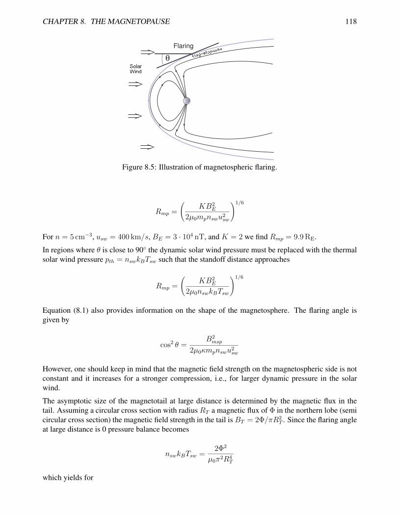
Figure 8.5: Illustration of magnetospheric flaring.

Rmp =

(KB2

E

2µ0mpnswu2sw

)1/6

For n = 5 cm−3, usw = 400 km/s, BE = 3 · 104 nT, and K = 2 we find Rmp = 9.9 RE.

In regions where θ is close to 90◦ the dynamic solar wind pressure must be replaced with the thermalsolar wind pressure pth = nswkBTsw such that the standoff distance approaches

Rmp =

(KB2

E

2µ0nswkBTsw

)1/6

Equation (8.1) also provides information on the shape of the magnetosphere. The flaring angle isgiven by

cos2 θ =B2msp

2µ0κmpnswu2sw

However, one should keep in mind that the magnetic field strength on the magnetospheric side is notconstant and it increases for a stronger compression, i.e., for larger dynamic pressure in the solarwind.

The asymptotic size of the magnetotail at large distance is determined by the magnetic flux in thetail. Assuming a circular cross section with radius RT a magnetic flux of Φ in the northern lobe (semicircular cross section) the magnetic field strength in the tail is BT = 2Φ/πR2

T . Since the flaring angleat large distance is 0 pressure balance becomes

nswkBTsw =2Φ2

µ0π2R4T

which yields for


Rmp =

(2Φ2

µ0π2nswkBTsw

)1/4

One can estimate this magnetic flux by the flux in the near Earth tail (at 30 RE distance with anaverage field of about 15 nT and a radius of about 20 RE . A more sophisticated estimate has toinclude the amount of open flux and the amount of flux which crosses the equatorial plane and doesnot go out to the distant (>100 RE) tail.

The magnetopause shape as discussed in this section uses a number of simplifications. Variations inthe location can also be caused by the structure (open or closed) of the magnetopause and by processesin the magnetosphere which re-arrange magnetic flux.

8.1.3 Magnetopause Motion, Thickness, and Plasma Properties

The magnetopause moves quite rapidly with speeds of several 10 km/s in- and outward (viewed fromthe Earth). Thus a spacecraft traverses the MP in general not because of the SC velocity but becauseof this rapid magnetopause motion. The cause for this motion are variation in the upstream solar windand changes in the magnetic field orientation which can lead to increasing or decreasing reconnectionrates.

N

Uz

Uy

By

Bx

10

30

-40

0

40

50

150

15

5

10

150

100

50

100

20

M’sheath MP M’sphereBL

Figure 8.6: Illustration of a typical magnetopause observation

The magnetopause thickness is typically around 800 km but can vary between about 100 km and 2000km. It is most easily identified in the subsolar dayside region. The structure is more turbulent and lessobvious at the flanks and at high latitudes. The identification of the magnetopause as a current layeris particularly difficult for cases where the magnetospheric and the magnetosheath magnetic fields arelargely aligned because the current density and field change is small.

A spacecraft entering the magnetosphere from the magnetosheath in the subsolar region (a regionwithin 5 or 6 RE of the subsolar point) would typically observe the following structure:


The plasma and the magnetic field in the magnetosheath are fairly disturbed. The SC encounterthe magnetopause as a sudden large change of the magnetic field orientation (and magnitude) in thedirection tangential to the magnetopause which is predominantly the y, z plane in GSM coordinates.The magnetic field turns predominantly into the northward z direction. At the magnetopause thedensity may decrease slightly. Typical for the region adjacent to the magnetopause is is a rotation(acceleration of the plasma velocity. This region of relatively fast flow and almost magnetosheathdensity is called the boundary layer and at low latitudes it is called the Low Latitude Boundary Layer(LLBL). The width of the LLBL is strongly varying and at times it may be entirely absent. Howevertypical for this region is a width of several thousand km with increasing width for increasing distancefrom the subsolar region. At the dawn-dusk terminator the width is typically half an RE .

8.2 Magnetopause Structure

8.2.1 Open or Closed Magnetopause Configuration

Locally there are various tests which can be applied to identify whether the magnetopause is open,i.e., whether there is a normal component of the magnetic field which connects the magnetosphericfield to the solar wind, or whether it is closed, i.e. the normal magnetic field is 0.

First we could attempt to determine the normal magnetic field component through the variance analy-sis. Since the variance analysis provides an estimate for the normal direction the magnetic field alongthis direction would be the normal field component. However, noting that the normal direction is notdetermined with perfect accuracy and that the magnetic field component in the normal direction isexpected to be small compared to the tangential field (the reasons for this will be discussed in the sec-tion on magnetic reconnection) any error in the normal direction would produce an apparent normalmagnetic field. Thus the variance analysis cannot be used to predict the normal magnetic field.

If a normal magnetic field were present and the magnetopause is a thin boundary than there is onlyone MHD discontinuity (which is not a shock) that is consistent with a normal field. This solution isthe rotational discontinuity. A rotational discontinuity has two properties which can be tested:

• DeHoffmann-Teller frame

• Nonlinear Alfvén wave

DeHoffmann-Teller frame

A DeHoffmann-Teller frame is a frame in which the convection electric field is 0 or

E = −u×B = 0

Consider a time interval with N measurements of the magnetic field and the velocity such the for anindividual measurement i the electric field is

E(i) = −u(i) ×B(i) = 0


Using a transformation into a frame moving with the velocity V relative to the satellite the electricfield becomes

E′(i) = −(u(i) −V

)×B(i) = 0

To determine the transformation velocity one has to minimize the quantity

D(V) =1

N

N∑i=1

∣∣∣E′(i)∣∣∣2 =∣∣∣(u(i) −V

)×B(i)

∣∣∣2

The minimum of this expression is obtained by∇VD(V) = 0 which yields

K0Vht =⟨K(i)u(i)

⟩or

Vht = K−10

⟨K(i)u(i)

⟩where 〈〉 denotes the average over all data point and

K(i)µν = B(i) 2

(δµν −

B(i)µ B

(i)ν

B(i) 2

)K0 =

⟨K(i)

⟩Note that this minimization does not automatically imply the existence of a good deHoffmann-Tellerframe. For a real plasma the average of the transformed electric field will never be exactly 0 but thequantity D(Vht) should be much smaller than for the originally measured velocities D(0).

A test for the deHoffmann-Teller frame is plotted in Figure (8.7) (right). Here the actual electric fieldis plotted versus the dHT electric field Eht = −Vht × B(i). Ideally the data point should exactlyline up along the diagonal (with slope 1). While this is not the case the data satisfies the relationvery closely. This implies that the configuration is electrostatic, i.e., ∂B/∂t = 0. All steady stateconfigurations belong to this group and in particular also a rotational discontinuity. The existence ofa good dHT frame is a necessary but not a sufficient condition for a rotational discontinuity.

Walen Relation

We know that a rotational discontinuity implies a change of the velocity by

∆u = ±∆vA = ±∆B√µ0ρ

This relation is called the Walen relation. It is valid for linear and nonlinear Alfvén waves (therotational discontinuity is a nonlinear Alfvén wave) and for switch-off slow shocks. With the trans-formation into the dHT frame the relation can also be written as


Figure 8.7: Tests of the deHoffmann-Teller frame and the Walen relation for the data set shown inFigure (8.3).

u(i) −Vht = ±v(i)A = ± B(i)√

µ0ρ(i)

for each data point in the rotational discontinuity where either the + or the − sign applies. Forthe data of Figure (8.3) the plot in Figure (8.7) shows that the Walen relation is not satisfied. Wetherefore conclude that the boundary is not an open boundary (or the configuration is not a goodone-dimensional current sheet).

8.2.2 MP Currents

Large Scale Magnetopause Current

Figure 8.8 shows an overview of the MP currents using the assumptions that the currents are pre-dominantly determined by the magnetospheric field adjacent to the magnetopause boundary. Themagnetopause current is largely perpendicular to the geomagnetic field if the magnetic field outsidethe magnetosphere is small.

The currents on the dayside magnetopause close through the tail magnetopause. In the magnetotailthe northern and the southern lobes are separated by a cross-tail current layer. This current also closesover the tail magnetopause. A word of caution is needed with respect to this concept of currentclosure. Although ∇ · j = 0, a particular current line will in general not close in the simplistic wayindicated in Figure 8.8. Currents do not originate in from some dipole as magnetic field lines and aregenerated locally. Thus any particular current line may be highly complicated and will in general not


B

J

Figure 8.8: Sketch of the MP currents.

close in a simple way into itself. There is also no simple concept like a frozen-in condition applicableto current density. Currents are not bound to a particle plasma element.

Local Magnetopause Current

The local origin of the magnetopause current can be understood from the basic particle dynamics.Ions impinging on the magnetosphere have a larger gyro-radius than the electrons (Figure 8.9). Be-cause of the larger gyroradius one expects them to determine the thickness of the magnetopauseto approximately the ion gyro-radius. Ions move opposite to the electrons in this boundary layer.This generates a surface current which separates the the magnetosheath from the magnetosphere andchange the magnetic field accordingly.

However, the typical magnetopause width is significantly larger than an ion gyro-radius (by about anorder of magnitude). The reason for this discrepancy are the collective plasma effects which are notincluded in the above simplified model. To better understand the magnetopause (and other currents inthe magnetosphere) we have to consider these collective effects for instance by using the fluid plasmaequations. For the resulting drifts it is often important to consider gyrotropic pressure.

Bmsh

=0

Bmsp

usw

jmp

EmpB

mp

+

rgi

-

rge

Magnetosphere

Magnetosheath

Magneto

pause

Figure 8.9: Illustration of particle dynamics at the magnetopause


Pressure Anisotropy

In many cases the pressure in the collisionless plasma of the magnetosphere is not isotropic. Howeverthe plasma is usually fairly gyrotropic meaning that it is well described by a parallel and perpendicularpressure. The reason for the gyrotropic pressure is the rapid gyro-motion which isotropizes the plasmamotion efficiently in the plane perpendicular to the magnetic field. In this case the pressure tensor canbe expressed as

p = p⊥1 + (p‖ − p⊥)BB

B2

Here as in the remainder of this subsection we have dropped an index s to indicate that the equationsare valid for each particle species in a plasma. For both pressures the ideal gas equation is a goodapproximation

p‖ = nkBT‖

p⊥ = nkBT⊥

If the adiabatic approximation is satisfied one can use the general definition of the adiabatic index

γ = (d+ 2)/d

with d being the degree of freedom. For the perpendicular motion we have d = 2 and for the parallelmotion d = 1 such that the adiabatic equations of state are

p‖ = p‖0

(n

n0

)3

p⊥ = p⊥0

(n

n0

)2

However, the adiabatic equations do not consider the coupling between the parallel and perpendicularpressures. For instance the perpendicular pressure should increase as a particle distribution move intoa region of larger magnetic field strength which is not the case for the adiabatic equations. Also thepressures are combined a measure for the internal energy such that the equations should satisfy energyconservation which is also not the case.

A better approximation can be found by considering the adiabatic invariants of single particle motion.Averaging the magnetic moment for a particle distribution function yields

〈µ〉 =kBT⊥B

=p⊥nB

Since the average magnetic moment must be conserved (if the particle gyro-motion is faster thanother temporal changes and the gyro radius is smaller than length scales of gradients in the plasma)the perpendicular adiabatic law is


d

dt

(p⊥nB

)= 0

The parallel adiabatic equation is more complicated and basically requires to consider energy conser-vations, i.e., it requires to integrate the collisionless Boltzmann equation for the parallel energy andfor the perpendicular energy separately. The resulting equations can be combined to

p⊥dp‖dt

+ 2p‖dp⊥dt

+ 5p⊥p‖∇ · u = 0 (8.2)

With the continuity equation

∇ · u =1

n

(∂n

∂t+ u · ∇n

)=

1

n

dn

dt

the pressure equation becomes

d

dt

(p‖p

2⊥

n5

)=

d

dt

(p‖B

2

n3

)= 0

With the ideal gas laws the equations of state can be re-written as

d

dt

(T⊥B

)= 0

d

dt

(B2T‖n2

)= 0

Thus a plasma which moves into a region of higher magnetic field strength will have an increasing per-pendicular and a decreasing parallel temperature. This is for instance the case for the magnetosheathplasma as it gets closer to the dayside magnetopause with the result of an increasing temperatureanisotropy.

Exercise: Show that the equation for the perpendicular kinetic energy is

∂∂t

(12ρu2⊥ + p⊥

)= −∇ ·

(12ρu2⊥ + p⊥

)u−∇ · p⊥u⊥ −∇ · L⊥ − qnu⊥ · E

Exercise: Show that the equation for the parallel kinetic energy is

∂∂t

(12ρu2‖ + p‖

)= −∇ ·

(12ρu2‖ + p‖

)u−∇ · p‖u‖ −∇ · L‖ − qnu‖ · E

Exercise: Show that by combining the above two equations and the momentum equations for paralleland perpendicular pressure one can derive equation 8.2.


Momentum Equation and and Fluid Particle Drifts

The fluid equation of motion for such a plasma is

ρs

(∂us∂t

+ us · ∇us

)= −∇ps⊥ −∇ ·

[(ps‖ − ps⊥)

BB

B2

]+ qsn(E + us ×B) (8.3)

Note that with a gyrotropic pressure the jump condition for the total pressure for plasma discontinu-ities becomes

p⊥ +B2

2µ0

= const

and the Walen relation for the normal velocity in rotational discontinuities becomes

un =

[(B2n

µ0ρ

)(1−

µ0(p‖ − p⊥)

B2

)]1/2

For a stationary plasma with sufficiently small velocities (such that the us ·∇us can be neglected) theforce balance equation is

qsn(E + us ×B) = ∇ps⊥ +∇ ·[(ps‖ − ps⊥)

BB

B2

]

Taking the cross-product of this equation with B/B2 and dividing by qsn yields

us =E×B

B2+

1

qsnB2B×∇ps⊥ +

1

qsnB2B×∇ ·

[(ps‖ − ps⊥)

BB

B2

](8.4)

which defines the fluid drifts in a stationary plasma configuration similar to the single particle driftsdiscussed earlier. The first term is the familiar E ×B drift which has to be present as a result of theLorentz transformation. The second and third terms are new and not present in this form in the singleparticle drifts. The new drifts arise due to the collective particle interactions.

The second term describes a particle drift perpendicular to the magnetic field and perpendicular tothe gradient of the perpendicular pressure. This drift is called the diamagnetic drift. and is present ifeither a gradient in the density or a gradient in the temperature of the plasma exist (or both).

Let us consider a gradient in the plasma number density as illustrated in Figure . Particle gyrate inthe magnetic field all in the same direction for the same charge. However, in the presence of a densitygradient there are more particle in the direction of the gradient than in the opposite direction. Thus anobserver at a fixed location would see more particle going in one direction (due to gyro-motion anddue to the larger number of particle in the density gradient direction) then in the opposite direction.Thus at a given location a net bulk velocity arises due to the density gradient. Note that this doesnot require for the center of gyro-motion to move. Similarly a gradient in the temperature results indifferent gyroradii in the direction of the gradient with the same net result for the bulk motion.

Since the diamagnetic drift velocity


B

n

Ions

J

Figure 8.10: Illustration of the diamagnetic drift

vdia,s =1

qsnB2B×∇ps⊥

depends on the charge electrons and ions move in opposite directions giving rise to a diamagneticcurrent

jdia = B×∇p⊥

with p⊥ = pe⊥ + pi⊥. If the plasma is isotropic the diamagnetic drift is the only plasma drift becauseps‖ = ps⊥.

For a non-isotropic plasma we can re-write the last term on the rhs of (8.4) using the radius of curva-ture definition as

vdia,s =ps‖ − ps⊥qsnB2Rc

B× n

where n is the outer normal of the field line curvature andRc is the radius of curvature. Thus this driftexists only for curved magnetic fields similar to the single particle curvature drift but it depends onparallel and perpendicular pressure and it can be positive or negative depending on the ratio of thesepressures. The corresponding current density is given by

jdia =p‖ − p⊥B2Rc

B× n

where p‖ = pe‖ + pi‖.

Applications of these drifts to the magnetopause are obvious If the magnetic field on the magne-tosheath side is weak then there has to be a pressure gradient in order to maintain an approximateequilibrium situation. The perpendicular pressure gradient drives a diamagnetic current which in turnaccounts self-consistently for the increase in magnetic field strength.

It should, however, be mentioned that the magnetic field in the magnetosheath is frequently not neg-ligible. In such cases the pressure gradient is usually small such that the diamagnetic currents aresmall. In these cases the current is mostly field-aligned.

Exercise: Show that a magnetic field rotation in the absence of a pressure gradient (i.e., equal mag-nitude magnetic fields on the two sides of the magnetopause) implies the the magnetopausecurrent is field-aligned.


Polarization Drifts

Thus far we have considered a stationary configuration. If there are slow changes in the configurationwe can compute the additional drifts by including the inertia term in the equation for the electric field

qsn(E + us ×B) = ∇ps⊥ +∇ ·[(ps‖ − ps⊥)

BB

B2

]+ ρs

∂us∂t

and by taking the cross-product with B/B2 and dividing by qsn obtain the additional term

vs =ms

qsB2B× ∂us

∂t

where we can substitute

∂us∂t

=∂

∂t

{E×B

B2+

1

qsnB2B×∇ps⊥ +

1

qsnB2B×∇ ·

[(ps‖ − ps⊥)

BB

B2

]}

For the first term this results in the guiding center polarization drift

vp,s =ms

qsB2

dE

dt

known from the single particle drifts. The second term yields a new polarization drift which in thecase of constant magnetic field and temperature results in

vpn,s =mskBTsq2sB

2∇⊥

d lnn

dt

Finally from generalized Ohm’s law one obtains a drift similar to the ones above from the currentinertia term:

vpc,s =me

ne2sB2B× ∂j

∂t

This drift is a motion of the bulk of the entire plasma such that it does not cause any current.

8.2.3 Observation of magnetopause reconnection

The observational verification of reconnection is difficult because a satellite provides only point mea-surements of usually complex plasma structure. Two major signatures are used to identify reconnec-tion at the magnetopause.

(a) On macro scales reconnection should generate open magnetic field which implies that the magne-topause is at time approximately a rotational discontinuity. In this case measurements of the plasmavelocity and magnetic field should satisfy approximately the so-called Walen relation


∆u = ±∆vA = ±∆B√µ0ρ

.

Where ∆u = u − uref with a measure velocity u and a reference measurement uref . While earlytests provided only few events which satisfied this relation later measurements with better temporalresolution provided many cases of thin magnetopause current layers which approximately satisfy theWalen relation [Sonnerup et al., 1981; Paschmann et al., 1986; Gosling et al., 1990]. An additionaltest for the presence of a stationary magnetopause structure is the presence of a dHT frame [Sonnerupet al., 1990]. Since the electric field is assumed constant there should be a reference frame in whichthe electric field is almost zero. An example which shows an excellent dHT frame but a poor Walentest is shown in Figure 8.7. The events typically are of short duration (few 10 seconds) indicating thinlayers, show a mixture of magnetosheath and magnetospheric plasma, and a occur mostly for strongsouthward IMF.

Dublicate of Figure 8.7 to be replaced by Walen relation plot showing reconnection!!!!!!!!!!!!!!!!!

Figure 8.11: Left: Example of FTE data after Russel and Elphic [1978].; Right:Sketch of a magneticflux rope and the magnetic field draping from Russel and Elphic [1978].

(b) The second class of events are so-called magnetic flux transfer events (FTE’s) [Haerendel et al.,1978; Russel and Elphic, 1978; Paschmann et al., 1982; Elphic, 1990, 1995]. They show typicallya strong bipolar variation of the magnetic field component normal to the magnetopause Bn togetherwith a mixture of magnetosheath and magnetospheric electron populations. Various other typicalproperties are a correlation with southward IMF, an increase of total pressure and total magneticfield, a strong rotation of the field in the core of the event, and a good dHT frame. The typical


duration is one to few minutes with a repetition rate of about 8 minutes. An example of FTE datais shown in Figure 8.11. The distribution of FTE’s indicates the subsolar region as their sourceregion. Furthermore typical amplitudes and scale sizes of FTE’s require fast reconnection, i.e., withthe Petschek reconnection rate.

-1.02

-0.86

-0.70

-0.54

-0.39

-12 -4 4 12x

0

30

60

90

120t = 120 s

Velocity, Field Lines and B_y

-12 -4 4 12

0

30

60

90

120

=

0.75z

-1.00

-0.84

-0.68

-0.52

-0.36

-12 -4 4 12x

0

30

60

90

120t = 150 s

-12 -4 4 12

0

30

60

90

120

=

0.86z

-0.97

-0.82

-0.66

-0.51

-0.35

-12 -4 4 12x

0

30

60

90

120t = 180 s

-12 -4 4 12

0

30

60

90

120

=

0.86z

-0.95

-0.80

-0.65

-0.50

-0.35

-12 -4 4 12x

0

30

60

90

120t = 210 s

-12 -4 4 12

0

30

60

90

120

=

1.13z

Figure 8.12: 2D simulation of localized reconnection.

8.2.4 Magnetopause Reconnection Models

The first explanation of FTE’s was suggested by Russel and Elphic [1978] who assumed that patchymagnetic reconnection generates a magnetic flux tube or rope which connects the magnetosphericand magnetosheath sides and thus contains magnetosheath and magnetospheric particles. Magneticfield draped around this tube can generate the bipolar Bn signature as the flux tube moves along themagnetopause boundary as illustrated in Figure 8.11.

There are various alternative models to explain FTE signature. The most basic possibility is a shortduration reconnection pulse in a two-dimensional approximation [Scholer, 1988; Southwood et al.,1988]. This process is illustrated as a result of a 2D MHD simulation in Figure 8.12. Here reconnec-tion generates a plasma bulge which and the magnetic field around this bulge will generate a bipolarBn signature.

Another model [Lee and Fu, 1985, 1986; Lee, 1995] employs reconnection at multiple x lines andthe magnetic islands moving along the magnetopause will also cause a bipolar Bn signature. Bothsingle x line reconnection model and multiple x line reconnection have also been simulated in three-dimensional models, i.e., with a finite (small) length of the reconnection region [Fu et al., 1990; Otto,1990; Schindler and Otto, 1990; Ma et al., 1994]. While the qualitative signatures are rather similar itappears that multiple x line reconnection and cases with relatively short x lines (3D) generate strongerand more realistic signatures. Currently it is unresolved whether reconnection occurs pulsed alonga rather long x line along much of the dayside magnetopause or at multiple patches [Nishida, 1989;Otto, 1991, 1995] distributed of the subsolar region of the magnetopause as illustrated in Figure 8.13.

Starting from very simple one-dimensional initial conditions, three-dimensional MHD simulations[Otto, 1999] demonstrate that reconnection initiated at a single reconnection site does not remains


BIMF

LinkedFlux

Free Flux

z

MSPB

y

Dayside reconnection (view from the sun)

Figure 8.13: Sketch of reconnection in a single reconnection region (left) or at multiple small recon-nection patches (right) in a view from the sun onto the dayside magnetopause.

localized. Rather the initial single reconnection site decays into multiple reconnection sites whichmove along the current sheet.

0.000

0.005

0.010

0.015

0.021Int. E_parallel

0

30

60

90

120

z

t=100

0.000

0.007

0.013

0.020

0.027t=378

Tot Pressure t=100

-50 -25 0 25 50

0

30

60

90

120

y

z

77.82

79.39

80.97

82.54

84.11t=378

-50 -25 0 25 50y

77.83

79.92

82.01

84.10

86.18

Figure 8.14: Parallel electric field distribution (top) and total pressure (bottom) from 3D MHD simu-lations of magnetic reconnection at an early (left) and a late (middle) time of the simulations. Right:magnetic flux ropes forming in the simulation.

Figure 8.14 shows the parallel electric field and the total pressure in the y, z plane at an early anda late time from a three-dimensional MHD simulation. Both quantities are integrated perpendicularto the current sheet (along x) to provide the global information which cannot be captures by a singlecut through the 3D system. The parallel electric field is chosen because it represents the individualdiffusion regions (reconnection sites) and maxima in the total pressure represent the locations withFTE-like properties. The initial configuration is a one-dimensional current sheet and reconnectionis triggered only at single location. The figure demonstrates that reconnection is not confined to the


initial onset location and FTE signatures develop in much of the simulation domain. The magneticfield configuration in Figure 8.14 shows two flux tubes elbow-like interlinked in the region of the totalpressure maximum (time t = 378).

B

B

B

x

V

V

x V

∆Φ1

∆Φ1

∆Φ2

∆Φ3

∆Φ2

∆Φ3

Midnight

tailward convection

sunwardconvection

Duskside flank

y

x

Figure 8.15: Left: Illustration of ionospheric convection and cross polar cap potential; Right: Sketchof the LLBL in the equatorial plane of the magnetosphere.

8.3 Viscous Interaction

From the early days of magnetospheric physics it has been presumed that viscosity at the magne-tospheric boundary may drive convection in the magnetosphere [Axford and Hines, 1961]. This isin particular evident from ionospheric convection. There is tailward convection in the polar cap atall times and only for strongly northward IMF two additional convection cells develop which showsome sunward flow driven by high latitude (cusp) reconnection. This indicates that a portion of themagnetospheric convection is always driven by the magnetosheath flow and it is mostly accepted thatabout 10 to 20 kV of the polar cap potential (Figure 8.15) may be attributed to viscous processes at themagnetospheric boundary. In other words some of the tailward flow in particular close to the centerof the convection cells may be on closed geomagnetic field lines.

In the outer magnetosphere the presence of the so-called low latitude boundary layer (LLBL, Fig-ure 8.15) is indicative for viscosity driven convection. The LLBL consists of a mixture of magneto-spheric and magnetosheath particles and plasma is flowing tailward although not quite as fast as inthe adjacent magnetosheath. It is not yet clear whether the LLBL is entirely on closed field lines oris actually a mixture of closed and open magnetic field [Newell and Meng, 2003]. On the daysideboundary magnetic reconnection may generate this boundary layer. The average width of the LLBLincreases away from the subsolar region to about 0.5 RE close to the terminator. A diffusion coeffi-cient of D = 109m2s−1 is required [Sonnerup, 1980] to account for the LLBL quantitatively by massand momentum diffusion .

The presence of viscosity in a fluid implies that momentum can be transported in a direction transverseto the actual flow. However, as pointed out the magnetospheric plasma is highly collisionless meaningthere are no classical collisions of particles in most of the magnetosphere. This leaves two mainphysical mechanisms which may account for the viscous coupling.

Micro-instabilities: The magnetosphere has rather thin boundaries. These boundaries imply largegradients in many plasma properties such as density, temperature, or magnetic field. The free en-


ergy either directly due to the strong gradients or caused by electron/ion beams at the boundary cancause various instabilities. The effect of such instabilities is to relax the configuration which causedthe instability which means to reduce the gradients or the fast relative motion of electrons and ions.Therefore they will cause diffusion of mass and momentum or friction similar to actual collisionsof particles. Various micro-instabilities such as lower hybrid drift modes, ion acoustic modes, ioncyclotron, etc. have been suggested to account for viscous interaction [La Belle and Treumann, 1988;Treumann and Baumjohann, 1997]. However, while there are models to evaluate the resulting trans-port or diffusion coefficient, there are no self-consistent models of the full nonlinear coupling. Thisis an important point because of the rather large width of the LLBL close to the terminator.

Kelvin Helmholtz (KH) waves: An alternative mechanism for the formation of the LLBL is theKelvin Helmholtz instability [Chandrasekhar, 1961]. This instability is present in many situationswhere two fluids stream relative to each other. Here the magnetosheath plasma (solar wind flow)moves fast relative to the plasma on the magnetospheric side which is almost at rest. Numericalsimulations have demonstrated that the KH can in principle operate at the magnetospheric flanks[Miura and Pritchett, 1982; Miura, 1982] and it is able to transport energy and momentum fromthe magnetosheath into the magnetosphere [Miura, 1984]. However, there are two aspects worthconsidering.

Growthrate of the KH instability (after Chandrasekhar):

q ={α1α2 [(V1 −V2) · k]2 − α1 [VA1 · k]2 − α2 [VA2 · k]2

}1/2Which yields the instability condition

[(V1 −V2) · k]2 >n1 + n2

µ0m0n1n2

[(B1 · k)2 + (B2 · k)2

]

The KH mode is stabilized by a variety of physical effects such as viscosity, surface tension, or amagnetic field aligned with the plasma flow. In the latter case the magnetic field is deformed by theplasma flow (Figure 8.16). This deformation requires additional energy such that the KH mode isstabilized [Chandrasekhar, 1961; Chen et al., 1997; Otto and Fairfield, 2000]. In fact if the magneticfield energy density is higher than the energy in the shear flow the KH mode cannot operate at all.

J

B

B

V

V

B

V

V

J

B

B

V

V

B

V

V

B

VA VA

Figure 8.16: Sketch of KH evolution in the presence of a magnetic field.

Vice versa reconnection has rather similar properties. Magnetic reconnection is stabilized by shearflow (Figure 8.17). The reason for this is that the information velocity for magnetic reconnection isthe Alfvén speed. Thus information that reconnection operates cannot propagate away from the x line


J

B

B

V

V

B

V

V

B

VA VA

Figure 8.17: Sketch of magnetic reconnection in the presence of sheared plasma flow.

if plasma flow is faster than the Alfvén speed such that reconnection cannot operate in the presence offast plasma flow Chen et al. [1997]; La Belle-Hamer et al. [1995]. Therefore reconnection requires∆VA > ∆v while the KH mode requires ∆v > VA,typ along the k vector of the instability.

In the equatorial plane the geomagnetic field is strongly northward. Thus the KH instability can op-erate in the equatorial plane if the IMF is mostly northward or southward. Many observations showquasi-periodic signatures of density, velocity and magnetic field fluctuations [Sckopke et al., 1981;Chen and Kivelson, 1993]. In a detailed study of such an event Fairfield et al. [2000] demonstratedthat these signature have a number of characteristic features (Figure 8.18). One of the most remark-able feature is the transient presence of negative Bz components although the geomagnetic and theinterplanetary magnetic field were strongly northward.

Figure 8.18: Three examples of quasi-periodic plasma and field signature from Fairfield et al. [2000].

In comparison two-dimensional MHD simulations (Figure 8.19) showed many of the same signaturesand it was possible to identify individual signatures for instance for the entrance and exit of the SCinto and out of the magnetosphere Otto and Fairfield [2000]. Particularly the twisting of the magneticfield in the KH vortex motion can generate negative Bz signature in small regions of space.

Simulation also demonstrated another important property of magnetic field deformation in the KHvortex. The KH mode is an ideal instability and therefore does not permit mass transport across


time = 58

-1.4

-0.6

0.2

1.0-2-1012

Plasma Velocity

∆x / RE

x

z

∆y / RE

Figure 8.19: Geometry for 2D MHD simulations at the magnetospheric boundary.

the magnetospheric boundary. As argued before the initial field is usually strongly parallel such thatreconnection cannot occur. However, the magnetic field deformation can generate strong local currentsheets in the KH vortices (Figure 8.20). Thus reconnection is possible within these small scale currentsheets Otto and Fairfield [2000].

B

B

B

V

V

V

V

B

B

B

MSHMSP

V

B

B

B

V

V

B

B

B

V

V

Figure 8.20: Schematic of the magnetic field deformation and subsequent reconnection inside KHvortices.

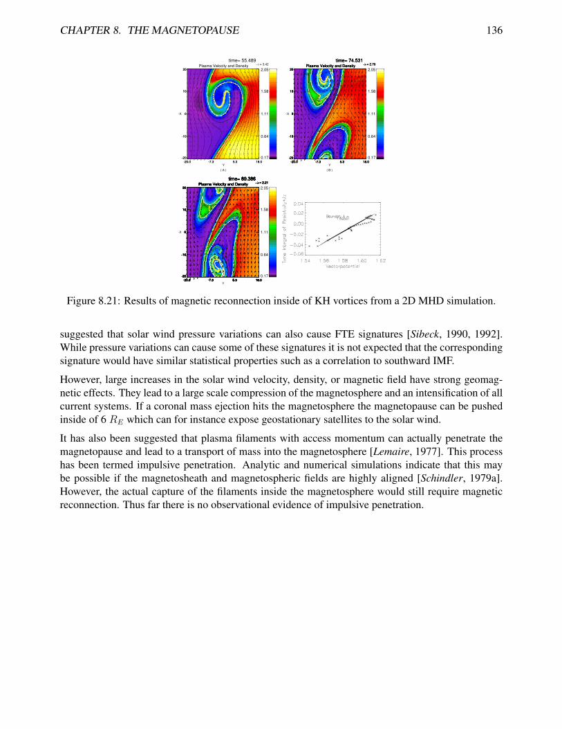
The mass transport into the magnetosphere for northward IMF is an unresolved problem. A possiblemechanism for this transport is reconnection at high latitudes (above the northern cusp and belowthe southern cusp) which can connect IMF with the magnetosphere and thus capture magnetosheathmaterial in the magnetosphere. An second plausible mechanism is reconnection inside KH vortices.In a quantitative evaluation of the reconnection inside of KH vortices (Figure 8.21) it is shown that thetransport rate is indeed sufficient to explain an effective mass diffusion coefficient of D = 109m2s−1

[Nykyri and Otto, 2001].

It should be remarked that the KH mode may also occur at other locations on the magnetosphericboundary than discussed here. In fact for any orientation of the IMF there are always locations onthe magnetospheric boundary where the magnetosheath and magnetospheric fields are approximatelyaligned.

Other processes at the magnetopause boundary Both magnetic reconnection and KH modes re-quire an boundary that unstable with respect to either mode. However, energy and momentum canalso be transferred by fluctuations carried by the solar wind or generated at the bow shock. It is


0.17

0.64

1.11

1.58

2.05

-20.0 -7.3Y

( A )

5.3 18.0

-20

-10

0-X

10

20 Plasma Velocity and Density

-20.0 -7.3 5.3 18.0

-20

-10

0

10

20

= 3.42time= 55.489

0.17

0.64

1.11

1.58

2.05

-20.0 -7.3 5.3Y

( B )

18.0

-20

-10

0-X

10


-20.0 -7.3 5.3 18.0

-20

-10

0

10

20

= 2.70time= 74.531

Plasma Velocity and Density

-20.0 -7.3 5.3 18.0

-20

-10

0

10

20

= 2.70time= 74.531

-x


-20.0 -7.3 5.3 18.0

-20

-10

0

10

20

= 2.70time= 74.531

0.17

0.64

1.11

1.58

2.05

-20.0 -7.3Y

5.3 18.0

-20

-10

-X 0

10


-20.0 -7.3 5.3 18.0

-20

-10

0

10

20

= 2.21time= 89.386


-20.0 -7.3 5.3 18.0

-20

-10

0

10

20

= 2.21time= 89.386


-20.0 -7.3 5.3 18.0

-20

-10

0

10

20

= 2.21time= 89.386


-20.0 -7.3 5.3 18.0

-20

-10

0

10

20

= 2.21time= 89.386


-20.0 -7.3 5.3 18.0

-20

-10

0

10

20

= 2.21time= 89.386

Figure 8.21: Results of magnetic reconnection inside of KH vortices from a 2D MHD simulation.

suggested that solar wind pressure variations can also cause FTE signatures [Sibeck, 1990, 1992].While pressure variations can cause some of these signatures it is not expected that the correspondingsignature would have similar statistical properties such as a correlation to southward IMF.

However, large increases in the solar wind velocity, density, or magnetic field have strong geomag-netic effects. They lead to a large scale compression of the magnetosphere and an intensification of allcurrent systems. If a coronal mass ejection hits the magnetosphere the magnetopause can be pushedinside of 6 RE which can for instance expose geostationary satellites to the solar wind.

It has also been suggested that plasma filaments with access momentum can actually penetrate themagnetopause and lead to a transport of mass into the magnetosphere [Lemaire, 1977]. This processhas been termed impulsive penetration. Analytic and numerical simulations indicate that this maybe possible if the magnetosheath and magnetospheric fields are highly aligned [Schindler, 1979a].However, the actual capture of the filaments inside the magnetosphere would still require magneticreconnection. Thus far there is no observational evidence of impulsive penetration.

chapter 8 the magnetopause - university of alaska...

Documents