TEL-AVIV UNIVERSITY

RAYMOND AND BEVERLY SACKLER

FACULTY OF EXACT SCIENCES

SCHOOL OF COMPUTER SCIENCE

Minkowski Sums of Simple Polygons

Thesis submitted in partial fulfillment of the requirements for the M.Sc.

degree in the School of Computer Science, Tel-Aviv University

by

Eduard Oks

The research work for this thesis has been carried out at Tel-Aviv University

under the supervision of Prof. Micha Sharir

June 2005

Abstract

Let P be a simple polygon with m edges, which is the disjoint union of k simple poly-gons, all monotone in a common direction u, and let Q be another simple polygon withn edges, which is the disjoint union of ℓ simple polygons, all monotone in a common di-rection v. We show that the combinatorial complexity of the Minkowski sum P ⊕ Q isO(kℓmnα(min{m,n})). Some structural properties of the case k = ℓ = 1 have been (im-plicitly) studied in [25]. We rederive these properties using a different proof, apply them toobtain the above complexity bound for k = ℓ = 1, obtain several additional properties of thesum for this special case, and then use them to derive the general bound.

2

Acknowledgments

I deeply thank Prof. Micha Sharir for his guidance and his tremendous help in preparingthis document. I also thank him for introducing me to the field of computational geometry.I also would like to thank Prof. Janos Pach for his help and contributions.

3

Contents

1 Introduction 5

1.1 The combinational complexity of Minkowski Sums . . . . . . . . . . . . . . . 6

1.2 Related Work . . . . . . . . . . . . . . . . . . . . . . . . . . . . . . . . . . . 7

1.2.1 Special cases of Minkowski sums . . . . . . . . . . . . . . . . . . . . . 7

1.2.2 Applications . . . . . . . . . . . . . . . . . . . . . . . . . . . . . . . . 10

1.3 Thesis Outline . . . . . . . . . . . . . . . . . . . . . . . . . . . . . . . . . . . 12

2 Minkowski Sums of Monotone Polygons 13

2.1 Separating Two Monotone Chains . . . . . . . . . . . . . . . . . . . . . . . . 14

2.2 Minkowski Sum of Two Monotone Polygons . . . . . . . . . . . . . . . . . . 17

2.3 The Boundary of the Sum of Two Monotone Polygons . . . . . . . . . . . . 19

2.4 Pockets in the Minkowski Sum of Monotone Polygons . . . . . . . . . . . . . 23

2.5 Minkowski Sum of Non-monotone Simple Polygons . . . . . . . . . . . . . . 29

2.6 Conclusion . . . . . . . . . . . . . . . . . . . . . . . . . . . . . . . . . . . . . 34

4

Chapter 1

Introduction

Given two sets P,Q ⊂ R2, their Minkowski sum, denoted by P ⊕ Q, is defined as the set

P ⊕ Q := {p + q | p ∈ P, q ∈ Q}.

This is a fundamental construct that arises in a wide range of applications, including robotmotion planning [5, 19], assembly planning [11], and computer-aided design and manufac-turing (CAD/CAM)[7].

Consider for example robot motion planning. This application involves placements andtranslational motion of an object in the presence of another object, which acts as a stationaryobstacle. Let Q denote the obstacle, and P the robot, which is only allowed to translate.Assuming, without loss of generality, that the origin o lies in P , and denoting by −P thereflection of P with respect to o, it follows by definition that K = (−P )⊕Q is the set of allvectors v such that translating P by v makes it intersect Q. In the study of motion plan-ning, this sum is called a configuration space obstacle, or C-obstacle. Hence the complementKc of K is a representation of the space of all free placements of P (namely, placementsdisjoint from Q). This observation makes Minkowski sums a central tool in the analysis oftranslational motion planning (see, e.g., [5, 23]), and we will also use this interpretation inour analysis.

1.1 The combinational complexity of Minkowski Sums

Motivated by these applications, there has been much work on obtaining sharp bounds onthe size of the Minkowski sums of two sets in two and three dimensions, and on developingfast algorithms for computing Minkowski sums. Throughout the thesis we only considerMinkowski sums of two polygons P , Q in the plane. It is well known that if both P and Qare convex polygons, with m and n vertices respectively, then P ⊕ Q is a convex polygonwith at most m + n vertices, and it can be computed in O(m + n) time [5]

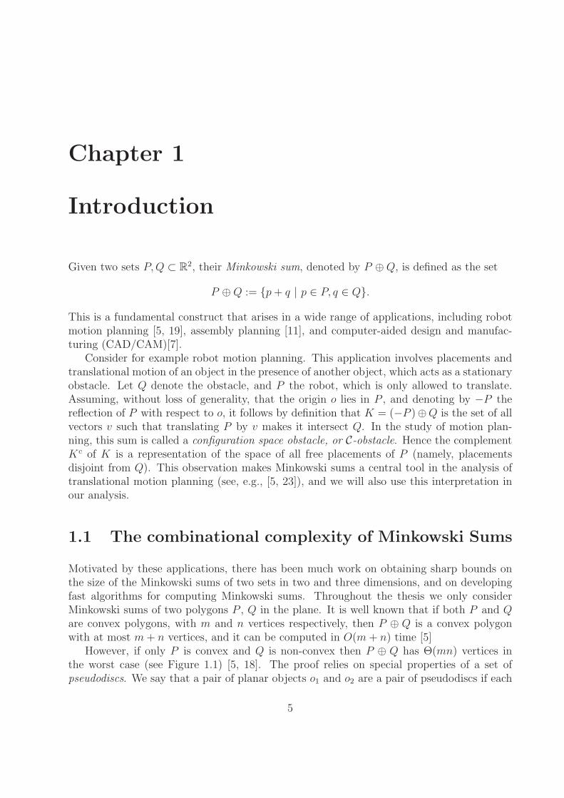
However, if only P is convex and Q is non-convex then P ⊕ Q has Θ(mn) vertices inthe worst case (see Figure 1.1) [5, 18]. The proof relies on special properties of a set ofpseudodiscs. We say that a pair of planar objects o1 and o2 are a pair of pseudodiscs if each

5

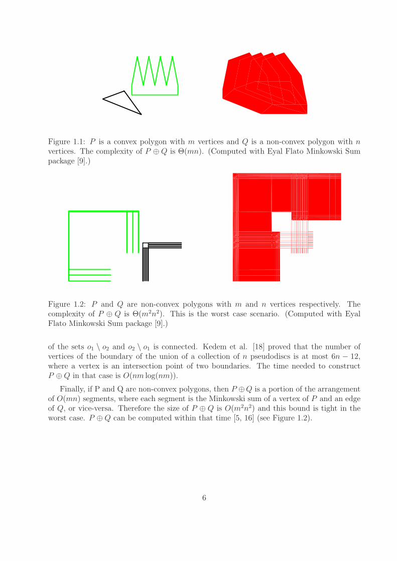
Figure 1.1: P is a convex polygon with m vertices and Q is a non-convex polygon with nvertices. The complexity of P ⊕ Q is Θ(mn). (Computed with Eyal Flato Minkowski Sumpackage [9].)

Figure 1.2: P and Q are non-convex polygons with m and n vertices respectively. Thecomplexity of P ⊕ Q is Θ(m2n2). This is the worst case scenario. (Computed with EyalFlato Minkowski Sum package [9].)

of the sets o1 \ o2 and o2 \ o1 is connected. Kedem et al. [18] proved that the number ofvertices of the boundary of the union of a collection of n pseudodiscs is at most 6n − 12,where a vertex is an intersection point of two boundaries. The time needed to constructP ⊕ Q in that case is O(nm log(nm)).

Finally, if P and Q are non-convex polygons, then P ⊕Q is a portion of the arrangementof O(mn) segments, where each segment is the Minkowski sum of a vertex of P and an edgeof Q, or vice-versa. Therefore the size of P ⊕ Q is O(m2n2) and this bound is tight in theworst case. P ⊕ Q can be computed within that time [5, 16] (see Figure 1.2).

6

1.2 Related Work

1.2.1 Special cases of Minkowski sums

In the previous section we presented the well known combinatorial bounds on the complexityof the Minkowski sum of two polygonal sets. In motion planning applications, one is ofteninterested in computing only a single connected component of the complement of P ⊕ Q[20]. Har-Peled et al. [14] showed that the complexity of a single face of the complementof P ⊕ Q is Θ(mnα(n)) in the worst case, where m and n are the number of vertices of Pand Q respectively (without loss of generality n < m), and α(·) is the functional inverse ofAckermann’s function [24].

The special case where P is a simple polygon and Q is a line segment has been recentlyanalyzed in [21], it was shown that in that case P ⊕ Q has at most 2n − 1 edges, and thisbound is tight in the worst case.

Ramkumar [22] presents a different approach to construct the outer face of the Minkowskisum. Existing methods rely on general algorithms for computing a single face in an arrange-ment of k line segments, which takes O(k(log k)(α(k))) time. Instead, his algorithm exploitsa new insight into the relationship between convolutions and Minkowski sums and, thoughasymptotically slower, has practical advantages for realistic polygon data. His method con-sists of traversing each cycle of the convolution, detecting self-intersections, and snippingoff the loops thus created. In order to detect self-intersections, the algorithm adapts thegeodesic triangulation ray-shooting data structure to answer ray-shooting queries on a dy-namic polygonal line of size n, in O(log2 n) amortized time. The algorithm constructs theouter face of the Minkowski sum of two simple polygons of size m and n, respectively, intime O((k +(m+n)

√l) log2(m+n)) where k is the size of the convolution (k can be O(mn)

in the worst case) and l is the number of cycles in the convolution.

De Berg and van der Stappen [6] report on results concerning the relation between thefatness of the Minkowski sum of two sets and the fatness of these sets. The fatness of anobject is determined by the emptiest ball centered inside the object and not fully containingit in its interior. Using this measure, they show that the fatness of A⊕B is at least as largeas min(fatness(A); fatness(B)), when A and B are connected closed and bounded sets inR

d .

Monotone Polygons

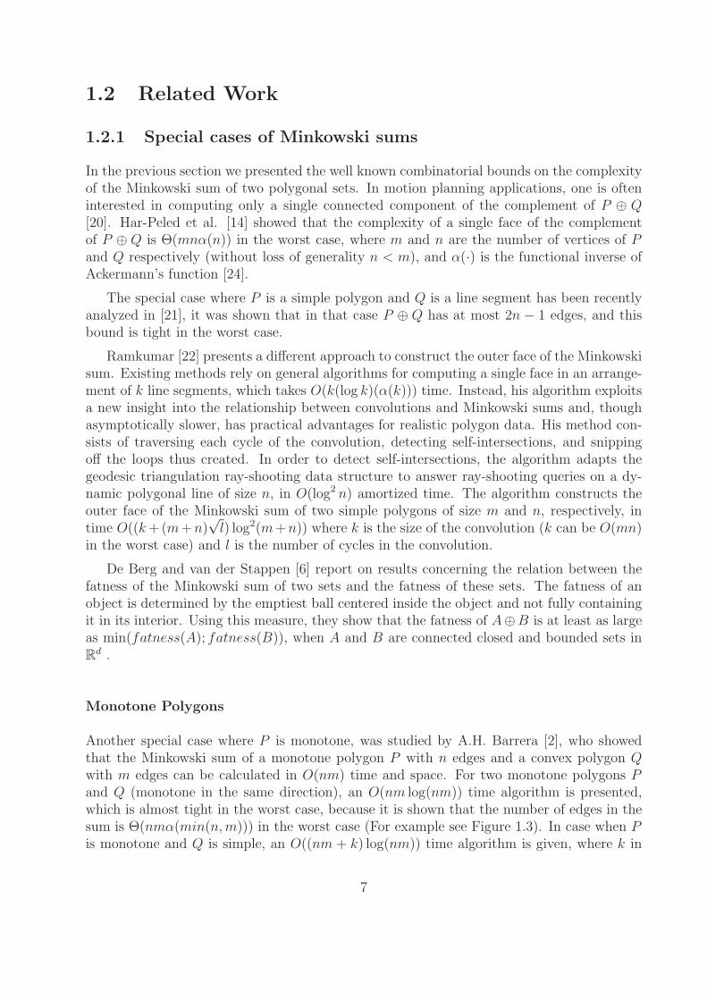
Another special case where P is monotone, was studied by A.H. Barrera [2], who showedthat the Minkowski sum of a monotone polygon P with n edges and a convex polygon Qwith m edges can be calculated in O(nm) time and space. For two monotone polygons Pand Q (monotone in the same direction), an O(nm log(nm)) time algorithm is presented,which is almost tight in the worst case, because it is shown that the number of edges in thesum is Θ(nmα(min(n,m))) in the worst case (For example see Figure 1.3). In case when Pis monotone and Q is simple, an O((nm + k) log(nm)) time algorithm is given, where k in

7

Figure 1.3: P and Q are x-monotone, non-convex polygons with m and n vertices respec-tively. The complexity of P ⊕ Q is Θ(nmα(min(n,m)) and the resulted polygon is x-monotone. (Computed with Eyal Flato Minkowski Sum package [9].)

the worst case can be Θ(n2m), and the number of edges in the sum is Θ(n2m). Barrera alsoproved that computing the Minkowski sum of two polygons is at least as hard as sorting X+ Y [3]. The best known time bound for solving this sorting problem is O(n2 log(n)), andit is an open problem whether this can be improved.

Discrete Approximations

Hartquist et al. [15] suggest a computing strategy for applications that use offsets, sweepsand Minkowski operations based on the ray-representation method. This method involvesclipping a given input to a grid of rays and applying the mathematical definitions and op-erators (such as Minkowski sums) on the resulting discrete set. The authors aim to solvemotion planning, process-modeling and visualization problems, and they present a hardwaredesign for those applications.

Kavraki [17] uses the Fast Fourier Transform (FFT) algorithm on the bitmaps of a robotand obstacles to find the corresponding configuration-space obstacles for the robot translatingamong the obstacles. This method approximates the configuration space obstacles. Themethod is inherently parallel and can benefit from existing experience and special hardwarefor computing the FFT.

1.2.2 Applications

The translational robot motion planning problem planning is a convenient case study forMinkowski sum algorithms, and we therefore detail it and use it as an example in the restof this thesis. There are many more applications in which the Minkowski sum operation isa useful tool. Some examples are listed here.

Polygon containment

Given two polygons P and Q in the plane, we wish to determine whether P can be contained(by translation, or by other geometric transformation) inside Q. This problem is known as

8

the polygon containment problem [4]. If we only allow a translation (namely, the orientationof P is fixed), the problem can be solved as follows: Consider the complement of Q as anobstacle for the robot P , and try to place P such that it does not penetrate this obstacle.Practically, let B be the bounding box of Q and let Qc = B \ Q be the complement of Q.The free placements for P inside Q can be found by computing Qc ⊕ (−P ).

Geographic Information Systems; Cartographic generalization

Geographic Information Systems (GIS) are increasingly being studied in computational ge-ometry. There are some problems in GIS that are closely related to our work. One of themwas first posed by Marc van Kreveld [26]: Given two simple polygons, P and Q with mand n edges respectively, find the minimum length translation of one polygon relative tothe other that will make the two polygons interior disjoint. The solution is based on thefact that P and Q are disjoint if and only if P ⊕ (−Q) does not contain the reference pointof Q. Assuming that in their original placement P and Q intersect and that the referencepoint of Q is at the origin o (we can assume this without loss of generality), the shortesttranslation of Q relative to P that separates them is given by the point on the boundary ofP ⊕ (−Q) which is closest to the origin o (this point can lie on the boundary of some holeof the Minkowski sum). The running time of this algorithm is Θ(n2m2) in the worst case,which is dominated by the complexity of the Minkowski sum algorithm.

Robust and efficient construction of planar Minkowski sums in practice

Flato and Halperin at [8, 10] present several different approaches to calculate the Minkowskisum of two simple polygons using the CGAL software library and its planar map pack-age. The algorithms decompose each of the polygons P,Q into convex sub-pieces, form theMinkowski sums of the separate pieces, and then construct the union of these sub-sums. Thealgorithms differ in the implementation of the union step – calculation of the union of theMinkowski sub-sums.In a subsequent work [1, 8] Agarwal, Flato and Halperin continue this research, by analyz-ing different decomposition methods, the first step of the Minkowski sum algorithm, such astriangulation, convex decomposition with/without Steiner points, approximations and heuris-tics. The emphasis of their work was to study the effect of the decomposition method onthe efficiency of the overall process.It is shown in these works that: (i) Triangulations are too costly. (ii) What constitutes agood decomposition for one of the input polygons depends on the other input polygon. Con-sequently, they develop a procedure for simultaneously decomposing the two polygons suchthat a “mixed” objective function is minimized. (iii) There are optimal decomposition algo-rithms that significantly expedite the Minkowski sum computation, but the decompositionitself is expensive to compute. In such cases, simple heuristics that approximate the optimaldecomposition seem to perform very well in practice. They examined several criteria thataffect the running time of the Minkowski sum algorithm. The most effective optimization is

9

minimizing the number of convex sub-polygons. Thus, triangulations which are widely usedin the theoretical literature are not practical for the Minkowski sum algorithms.

1.3 Thesis Outline

The thesis presents a general technique for analyzing the complexity of the Minkowski sumof two simple polygons, using their partition into monotone pieces.

Specifically, let P be a simple polygon with m edges, which is the disjoint union ofk simple polygons, all monotone in a common direction u, and let Q be another simplepolygon with n edges, which is the disjoint union of ℓ simple polygons, all monotone ina common direction v. In Chapter 2 we show that the combinatorial complexity of theMinkowski sum P ⊕ Q is O(kℓmnα(min{m,n})). Some structural properties of the casek = ℓ = 1 have been (implicitly) studied by Toussaint and ElGindy [25]. We re-derive theseproperties using a different proof and apply them to obtain the above complexity bound fork = ℓ = 1. We obtain additional properties of the sum for this special case. Specifically, weshow that the boundary of the Minkowski sum is the concatenation of two u-monotone andtwo v-monotone connected polygonal chains which are pairwise openly disjoint, and that thenumber of pockets in P ⊕ Q is O(m + n). At the end we use all these properties to derivethe complexity of the sum for the general case. (A pocket is a maximal sub-chain of theboundary that is monotone in one of the directions u, v and has unique local minimum ormaximum in the other direction.) The bound is worst-case tight for k = ℓ = 1, as followsfrom the construction of Barrera [2], and is almost tight in the general case k = Θ(m),ℓ = Θ(n).

We give concluding remarks and suggest for further research in Section 2.6.

10

Chapter 2

Minkowski Sums of Monotone

Polygons

In this chapter we study the coplexity of the Minkowski sum of two simple polygons, andexpress it in terms of the number of monotone sub-polygons into which each of them can bedecomposed.

A simple polygon P is said to be monotone in direction u (also referred to as u-monotone)if every line orthogonal to u intersects P in a connected (possibly empty) interval. We candecompose any simple polygon P with m edges into simple sub-polygons, all monotone insome specified direction u, by drawing a vertical segment through each vertex of P whichis a locally u-extremal point of ∂P , and by extending that segment inside P till it hits ∂Pagain. These segments decompose P into O(m) pairwise openly disjoint u-monotone simplepolygons, and this bound is tight in the worst case.

Let P be a u-monotone simple polygon with m edges, and let Q be a v-monotone simplepolygon with n edges, for two (possibly different) directions u, v. We show (Theorem 2.2.1)that the complexity of P ⊕Q in this case is only O(mnα(min{m,n})), which is tight in theworst case. (The upper bound was obtained by Barrera [2] for the special case u = v. Healso showed that the lower bound can be attained in this case.)

The proof relies on the following separation property, due to Toussaint and ElGindy [25]:Given disjoint monotone polygons P and Q as above, we can translate P to infinity, withoutcolliding with Q, in at least one of the four directions u ± π/2, v ± π/2. This propertyimplies that P ⊕ Q is simply connected, from which the complexity bound follows usingknown bounds on the complexity of a single face in an arrangement of line segments; see,e.g., [24].

We provide, in Theorem 2.1.1, an alternative proof of the result of [25], and then use itto obtain the asserted complexity bound. Moreover, we derive several additional structuralproperties of the sum P ⊕Q of two monotone simple polygons. For example, we show that itsboundary is the concatenation of four connected portions, two of which are u-monotone andtwo v-monotone. We also show that the number of pockets along ∂(P ⊕Q) is only O(m+n).This notion will be defined and analyzed in Section 2.4. This is roughly equivalent to

11

asserting that the number of points on ∂(P ⊕ Q) that are locally x-extremal or y-extremalis O(m + n).

We next use all these properties to prove the main result of the paper, which asserts that,if P is a simple polygon with m edges which is the disjoint union of k simple u-monotonesub-polygons, and Q is a simple polygon with n edges which is the disjoint union of ℓ simplev-monotone sub-polygons, for any (possibly distinct) directions u, v, then the complexityof P ⊕ Q is O(kℓmnα(min{m,n})). This (almost) properly interpolates between the twoextreme cases k = ℓ = 1 (where the bound is worst case tight), and k = Θ(m), ℓ = Θ(n)(where we get an extra α(·) factor).

2.1 Separating Two Monotone Chains

Theorem 2.1.1 (slightly reformulated) was already proven in [25]. We present here a differentproof, using a functional representation of monotone polygonal paths.1

Theorem 2.1.1 Let f(x) : [a, b] 7→ IR, g(y) : [c, d] 7→ IR be (graphs of) continuous realfunctions defined on the above intervals of the x- and y-axes, respectively, that do not inter-sect each other. Then f(x) can be translated to infinity along at least one of the four axisdirections without colliding with g(y).

We say that a point p of the plane is directly to the right of another point q if the half-linestarting at q and pointing to the positive x-direction passes through p. The notions of beingdirectly to the left, directly above, and directly below, are defined in an analogous manner.

Lemma 2.1.2 Suppose that g(y) has a point directly to the right of the right endpoint off(x). Then g(y) has no point directly to the left of any point of f(x).

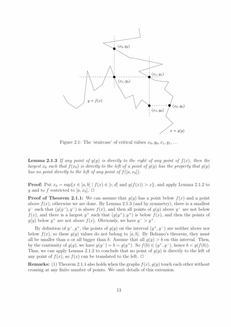
Proof: It is enough to show, by symmetry, that this holds for every y ≥ f(b). If for everyy ≥ f(b) we have g(y) > b, we are done. Otherwise, set x0 := g(f(b)), y0 := f(b), x1 := b.If there exist y ≥ f(b) with g(y) ≤ b, then denote by y1 the infimum of all such y. Then,by continuity, g(y1) = x1, and the statement (that g(y) has no point directly to the left ofany point of f(x)) holds on the interval [y0, y1]. If f(x) remains under y1 in every point tothe left of x0, then the statement holds on the whole interval [y0, d]. Otherwise, there is alargest x2 where (proceeding from right to left) f(x) first attains y1. Similarly, now g(y)either remains to the right of x2 all the way to the end (d, g(d)), or there exists y2 whereg(y) first reaches x2. See Figure 2.1.

This alternating construction terminates in finitely many steps, for otherwise we wouldobtain a bounded sequence (x0, y0), (x1, y0), (x1, y1), (x2, y1), (x2, y2), . . ., monotone in bothcoordinates, and its limit would be a common point of f(x) and g(y). It is easily seen thatthe termination of the process implies the statement of the lemma over the interval [y0, d],and a symmetric argument implies it for [c, y0]. 2

1We are grateful to Janos Pach for suggesting this proof, which has simplified our earlier analysis.

12

(x1, y1)

(x0, y0)

x = g(y)

(x1, y0)

(x2, y2)

(x1, y2)

y = f(x)

Figure 2.1: The ‘staircase’ of critical values x0, y0, x1, y1, . . .

Lemma 2.1.3 If any point of g(y) is directly to the right of any point of f(x), then thelargest x0 such that f(x0) is directly to the left of a point of g(y) has the property that g(y)has no point directly to the left of any point of f([a, x0]).

Proof: Put x0 = sup{x ∈ [a, b] | f(x) ∈ [c, d] and g(f(x)) > x}, and apply Lemma 2.1.2 tog and to f restricted to [a, x0]. 2

Proof of Theorem 2.1.1: We can assume that g(y) has a point below f(x) and a pointabove f(x), otherwise we are done. By Lemma 2.1.3 (and by symmetry), there is a smallesty− such that (g(y−), y−) is above f(x), and then all points of g(y) above y− are not belowf(x), and there is a largest y+ such that (g(y+), y+) is below f(x), and then the points ofg(y) below y+ are not above f(x). Obviously, we have y− > y+.

By definition of y−, y+, the points of g(y) on the interval (y+, y−) are neither above norbelow f(x), so these g(y) values do not belong to [a, b]. By Bolzano’s theorem, they mustall be smaller than a or all bigger than b. Assume that all g(y) > b on this interval. Then,by the continuity of g(y), we have g(y−) = b = g(y+). So f(b) ∈ (y+, y−), hence b < g(f(b)).Thus, we can apply Lemma 2.1.2 to conclude that no point of g(y) is directly to the left ofany point of f(x), so f(x) can be translated to the left. 2

Remarks: (1) Theorem 2.1.1 also holds when the graphs f(x), g(y) touch each other withoutcrossing at any finite number of points. We omit details of this extension.

13

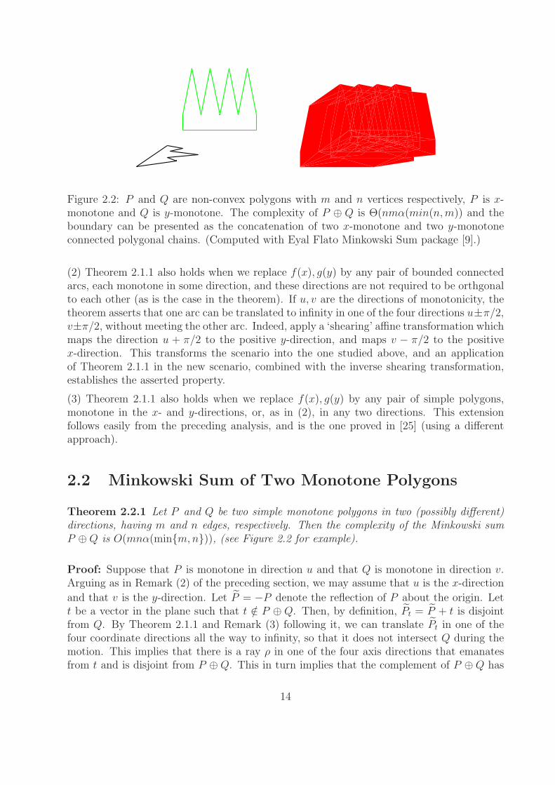
Figure 2.2: P and Q are non-convex polygons with m and n vertices respectively, P is x-monotone and Q is y-monotone. The complexity of P ⊕ Q is Θ(nmα(min(n,m)) and theboundary can be presented as the concatenation of two x-monotone and two y-monotoneconnected polygonal chains. (Computed with Eyal Flato Minkowski Sum package [9].)

(2) Theorem 2.1.1 also holds when we replace f(x), g(y) by any pair of bounded connectedarcs, each monotone in some direction, and these directions are not required to be orthgonalto each other (as is the case in the theorem). If u, v are the directions of monotonicity, thetheorem asserts that one arc can be translated to infinity in one of the four directions u±π/2,v±π/2, without meeting the other arc. Indeed, apply a ‘shearing’ affine transformation whichmaps the direction u + π/2 to the positive y-direction, and maps v − π/2 to the positivex-direction. This transforms the scenario into the one studied above, and an applicationof Theorem 2.1.1 in the new scenario, combined with the inverse shearing transformation,establishes the asserted property.

(3) Theorem 2.1.1 also holds when we replace f(x), g(y) by any pair of simple polygons,monotone in the x- and y-directions, or, as in (2), in any two directions. This extensionfollows easily from the preceding analysis, and is the one proved in [25] (using a differentapproach).

2.2 Minkowski Sum of Two Monotone Polygons

Theorem 2.2.1 Let P and Q be two simple monotone polygons in two (possibly different)directions, having m and n edges, respectively. Then the complexity of the Minkowski sumP ⊕ Q is O(mnα(min{m,n})), (see Figure 2.2 for example).

Proof: Suppose that P is monotone in direction u and that Q is monotone in direction v.Arguing as in Remark (2) of the preceding section, we may assume that u is the x-direction

and that v is the y-direction. Let P = −P denote the reflection of P about the origin. Lett be a vector in the plane such that t /∈ P ⊕ Q. Then, by definition, Pt = P + t is disjointfrom Q. By Theorem 2.1.1 and Remark (3) following it, we can translate Pt in one of thefour coordinate directions all the way to infinity, so that it does not intersect Q during themotion. This implies that there is a ray ρ in one of the four axis directions that emanatesfrom t and is disjoint from P ⊕ Q. This in turn implies that the complement of P ⊕ Q has

14

no bounded components (‘holes’ of P ⊕ Q), and thus P ⊕ Q is simply connected.

In other words, the boundary of P ⊕ Q is connected, and coincides with the boundaryof the unbounded face of its complement. Let Σ denote the set of all line segments of theform e + v, where e is an edge of P and v is a vertex of Q, or e is an edge of Q and v is avertex of P . Σ consists of 2mn segments, and any point on ∂(P ⊕ Q) must be contained inone of these segments. As is well known (see, e.g., [24]), the complexity of any single face inan arrangement of 2mn segments is O(mnα(mn)). To obtain the slightly improved assertedbound, assume, without loss of generality, that m ≤ n. Note that Σ can be represented asthe union of 2m subsets, each consisting of the sums of all edges of Q with a fixed vertex ofP , or of the sums of all vertices of Q with a fixed edge of P . Each subset consists of pairwise(openly) disjoint segments, so the complexity of the sub arrangement that they form is O(n).We then apply the Combination Lemma of Har-Peled [13], which implies that the complexityof a single face in the overlay of 2m arrangements, each of complexity O(n), is O(mnα(m)).See also [?] for an alternative proof. 2

2.3 The Boundary of the Sum of Two Monotone Poly-

gons

In what follows, we assume that P and Q are monotone in the x- and y-directions, respec-tively. As noted above, this involves no loss of generality.

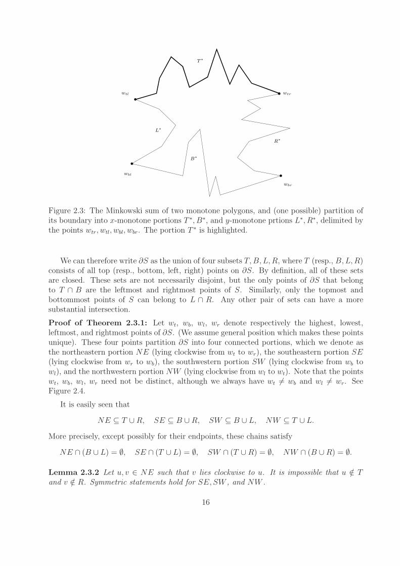
Theorem 2.3.1 Let P and Q be two simple polygons monotone in the x- and the y-directions,respectively. Then the boundary of S = P ⊕ Q is the concatenation of two x-monotone andtwo y-monotone connected polygonal chains, which are pairwise openly disjoint.

See Figure 2.3.

We use in the proof the interpretation, already mentioned above, of S = P ⊕ Q as thespace of all “forbidden” translations of P = (−P ) at which it intersects Q, which we regard

as stationary. The boundary of S is the set of all translations where P touches Q, but doesnot intersect its interior.

By Theorem 2.1.1, each point v ∈ ∂S can be classified into one (or more) of the fourfollowing types:

Top, if P can be moved from v to infinity in the positive y-direction without penetratinginto Q.

Bottom, if P can be moved from v to infinity in the negative y-direction without penetratinginto Q.

Left, if P can be moved from v to infinity in the negative x-direction without penetratinginto Q.

Right, if P can be moved from v to infinity in the positive x-direction without penetratinginto Q.

15

B∗

L∗

R∗

T∗

wtrwtl

wbl

wbr

Figure 2.3: The Minkowski sum of two monotone polygons, and (one possible) partition ofits boundary into x-monotone portions T ∗, B∗, and y-monotone prtions L∗, R∗, delimited bythe points wtr, wtl, wbl, wbr. The portion T ∗ is highlighted.

We can therefore write ∂S as the union of four subsets T,B, L,R, where T (resp., B,L,R)consists of all top (resp., bottom, left, right) points on ∂S. By definition, all of these setsare closed. These sets are not necessarily disjoint, but the only points of ∂S that belongto T ∩ B are the leftmost and rightmost points of S. Similarly, only the topmost andbottommost points of S can belong to L ∩ R. Any other pair of sets can have a moresubstantial intersection.

Proof of Theorem 2.3.1: Let wt, wb, wl, wr denote respectively the highest, lowest,leftmost, and rightmost points of ∂S. (We assume general position which makes these pointsunique). These four points partition ∂S into four connected portions, which we denote asthe northeastern portion NE (lying clockwise from wt to wr), the southeastern portion SE(lying clockwise from wr to wb), the southwestern portion SW (lying clockwise from wb towl), and the northwestern portion NW (lying clockwise from wl to wt). Note that the pointswt, wb, wl, wr need not be distinct, although we always have wt 6= wb and wl 6= wr. SeeFigure 2.4.

It is easily seen that

NE ⊆ T ∪ R, SE ⊆ B ∪ R, SW ⊆ B ∪ L, NW ⊆ T ∪ L.

More precisely, except possibly for their endpoints, these chains satisfy

NE ∩ (B ∪ L) = ∅, SE ∩ (T ∪ L) = ∅, SW ∩ (T ∪ R) = ∅, NW ∩ (B ∪ R) = ∅.

Lemma 2.3.2 Let u, v ∈ NE such that v lies clockwise to u. It is impossible that u /∈ Tand v /∈ R. Symmetric statements hold for SE, SW , and NW .

16

wrt

wtr

wrb

wbl

B∗

L∗

R∗

T∗

wtl

wbr

wlt

wlb

wt

wr

wl

wb

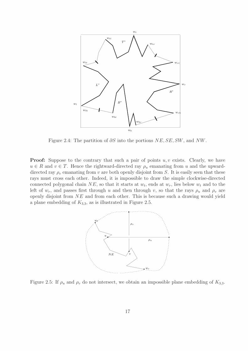
Figure 2.4: The partition of ∂S into the portions NE,SE, SW , and NW .

Proof: Suppose to the contrary that such a pair of points u, v exists. Clearly, we haveu ∈ R and v ∈ T . Hence the rightward-directed ray ρu emanating from u and the upward-directed ray ρv emanating from v are both openly disjoint from S. It is easily seen that theserays must cross each other. Indeed, it is impossible to draw the simple clockwise-directedconnected polygonal chain NE, so that it starts at wt, ends at wr, lies below wt and to theleft of wr, and passes first through u and then through v, so that the rays ρu and ρv areopenly disjoint from NE and from each other. This is because such a drawing would yielda plane embedding of K3,3, as is illustrated in Figure 2.5.

wt

wr

u

vNE

ρu

ρv

Figure 2.5: If ρu and ρv do not intersect, we obtain an impossible plane embedding of K3,3.

17

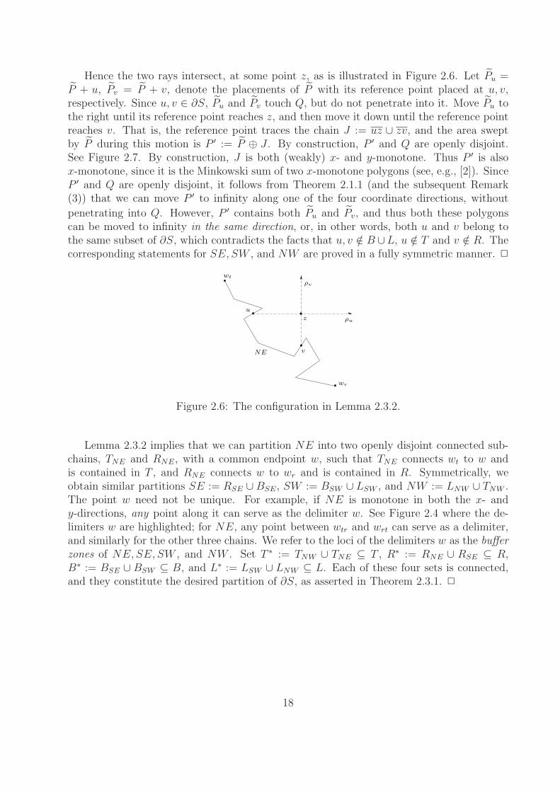
Hence the two rays intersect, at some point z, as is illustrated in Figure 2.6. Let Pu =P + u, Pv = P + v, denote the placements of P with its reference point placed at u, v,respectively. Since u, v ∈ ∂S, Pu and Pv touch Q, but do not penetrate into it. Move Pu tothe right until its reference point reaches z, and then move it down until the reference pointreaches v. That is, the reference point traces the chain J := uz ∪ zv, and the area sweptby P during this motion is P ′ := P ⊕ J . By construction, P ′ and Q are openly disjoint.See Figure 2.7. By construction, J is both (weakly) x- and y-monotone. Thus P ′ is alsox-monotone, since it is the Minkowski sum of two x-monotone polygons (see, e.g., [2]). SinceP ′ and Q are openly disjoint, it follows from Theorem 2.1.1 (and the subsequent Remark(3)) that we can move P ′ to infinity along one of the four coordinate directions, without

penetrating into Q. However, P ′ contains both Pu and Pv, and thus both these polygonscan be moved to infinity in the same direction, or, in other words, both u and v belong tothe same subset of ∂S, which contradicts the facts that u, v /∈ B ∪L, u /∈ T and v /∈ R. Thecorresponding statements for SE, SW , and NW are proved in a fully symmetric manner. 2

wt

wr

u

vNE

ρu

ρv

z

Figure 2.6: The configuration in Lemma 2.3.2.

Lemma 2.3.2 implies that we can partition NE into two openly disjoint connected sub-chains, TNE and RNE, with a common endpoint w, such that TNE connects wt to w andis contained in T , and RNE connects w to wr and is contained in R. Symmetrically, weobtain similar partitions SE := RSE ∪ BSE, SW := BSW ∪ LSW , and NW := LNW ∪ TNW .The point w need not be unique. For example, if NE is monotone in both the x- andy-directions, any point along it can serve as the delimiter w. See Figure 2.4 where the de-limiters w are highlighted; for NE, any point between wtr and wrt can serve as a delimiter,and similarly for the other three chains. We refer to the loci of the delimiters w as the bufferzones of NE,SE, SW , and NW . Set T ∗ := TNW ∪ TNE ⊆ T , R∗ := RNE ∪ RSE ⊆ R,B∗ := BSE ∪ BSW ⊆ B, and L∗ := LSW ∪ LNW ⊆ L. Each of these four sets is connected,and they constitute the desired partition of ∂S, as asserted in Theorem 2.3.1. 2

18

Q

zu

v

J

Pu

Pv

P ′

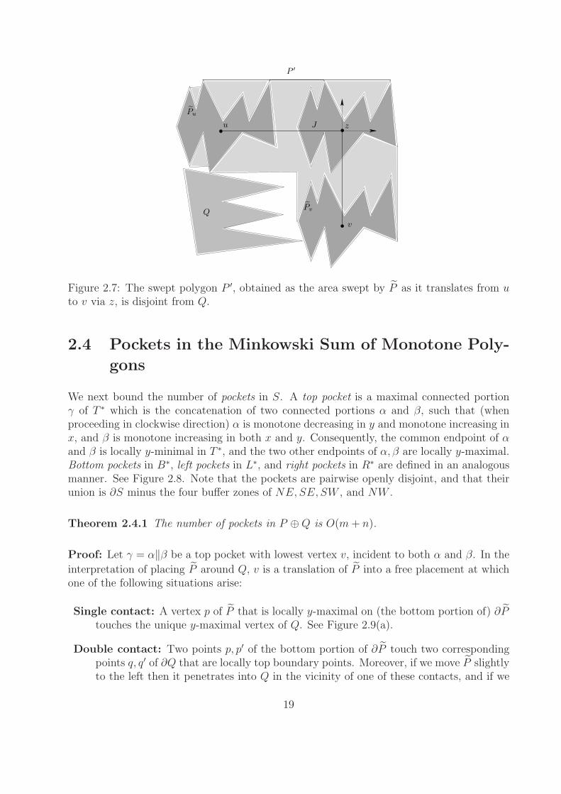
Figure 2.7: The swept polygon P ′, obtained as the area swept by P as it translates from uto v via z, is disjoint from Q.

2.4 Pockets in the Minkowski Sum of Monotone Poly-

gons

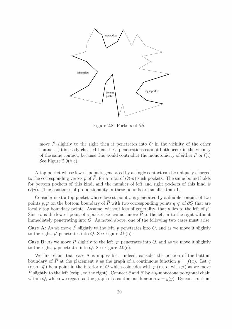
We next bound the number of pockets in S. A top pocket is a maximal connected portionγ of T ∗ which is the concatenation of two connected portions α and β, such that (whenproceeding in clockwise direction) α is monotone decreasing in y and monotone increasing inx, and β is monotone increasing in both x and y. Consequently, the common endpoint of αand β is locally y-minimal in T ∗, and the two other endpoints of α, β are locally y-maximal.Bottom pockets in B∗, left pockets in L∗, and right pockets in R∗ are defined in an analogousmanner. See Figure 2.8. Note that the pockets are pairwise openly disjoint, and that theirunion is ∂S minus the four buffer zones of NE,SE, SW , and NW .

Theorem 2.4.1 The number of pockets in P ⊕ Q is O(m + n).

Proof: Let γ = α‖β be a top pocket with lowest vertex v, incident to both α and β. In the

interpretation of placing P around Q, v is a translation of P into a free placement at whichone of the following situations arise:

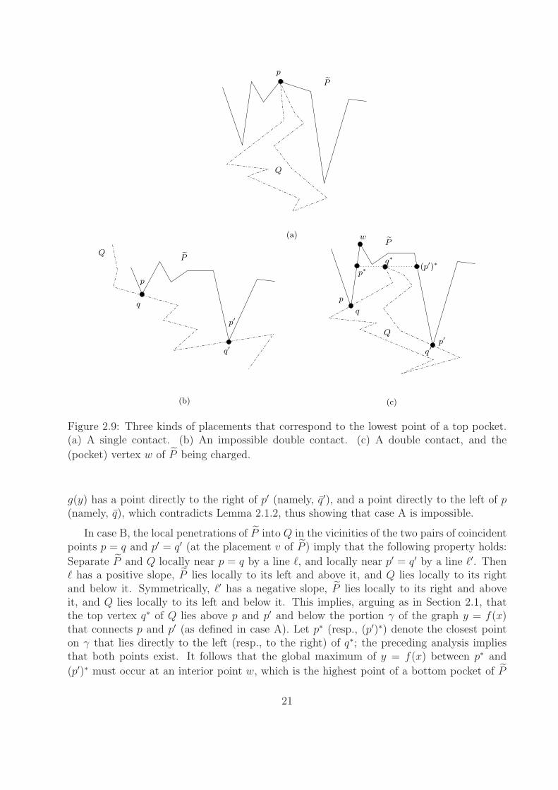
Single contact: A vertex p of P that is locally y-maximal on (the bottom portion of) ∂Ptouches the unique y-maximal vertex of Q. See Figure 2.9(a).

Double contact: Two points p, p′ of the bottom portion of ∂P touch two correspondingpoints q, q′ of ∂Q that are locally top boundary points. Moreover, if we move P slightlyto the left then it penetrates into Q in the vicinity of one of these contacts, and if we

19

left pocket

bottompocket

top pocket

right pocket

Figure 2.8: Pockets of ∂S.

move P slightly to the right then it penetrates into Q in the vicinity of the othercontact. (It is easily checked that these penetrations cannot both occur in the vicinityof the same contact, because this would contradict the monotonicity of either P or Q.)See Figure 2.9(b,c).

A top pocket whose lowest point is generated by a single contact can be uniquely chargedto the corresponding vertex p of P , for a total of O(m) such pockets. The same bound holdsfor bottom pockets of this kind, and the number of left and right pockets of this kind isO(n). (The constants of proportionality in these bounds are smaller than 1.)

Consider next a top pocket whose lowest point v is generated by a double contact of twopoints p, p′ on the bottom boundary of P with two corresponding points q, q′ of ∂Q that arelocally top boundary points. Assume, without loss of generality, that p lies to the left of p′.Since v is the lowest point of a pocket, we cannot move P to the left or to the right withoutimmediately penetrating into Q. As noted above, one of the following two cases must arise:

Case A: As we move P slightly to the left, p penetrates into Q, and as we move it slightlyto the right, p′ penetrates into Q. See Figure 2.9(b).

Case B: As we move P slightly to the left, p′ penetrates into Q, and as we move it slightlyto the right, p penetrates into Q. See Figure 2.9(c).

We first claim that case A is impossible. Indeed, consider the portion of the bottomboundary of P at the placement v as the graph of a continuous function y = f(x). Let q(resp., q′) be a point in the interior of Q which coincides with p (resp., with p′) as we move

P slightly to the left (resp., to the right). Connect q and q′ by a y-monotone polygonal chainwithin Q, which we regard as the graph of a continuous function x = g(y). By construction,

20

Q

q

q′

P

(b) (c)

Q

Q

q

q′

P(a)

P

p

p

p′

p

w

p′

q∗

p∗(p′)∗

Figure 2.9: Three kinds of placements that correspond to the lowest point of a top pocket.(a) A single contact. (b) An impossible double contact. (c) A double contact, and the

(pocket) vertex w of P being charged.

g(y) has a point directly to the right of p′ (namely, q′), and a point directly to the left of p(namely, q), which contradicts Lemma 2.1.2, thus showing that case A is impossible.

In case B, the local penetrations of P into Q in the vicinities of the two pairs of coincidentpoints p = q and p′ = q′ (at the placement v of P ) imply that the following property holds:

Separate P and Q locally near p = q by a line ℓ, and locally near p′ = q′ by a line ℓ′. Thenℓ has a positive slope, P lies locally to its left and above it, and Q lies locally to its rightand below it. Symmetrically, ℓ′ has a negative slope, P lies locally to its right and aboveit, and Q lies locally to its left and below it. This implies, arguing as in Section 2.1, thatthe top vertex q∗ of Q lies above p and p′ and below the portion γ of the graph y = f(x)that connects p and p′ (as defined in case A). Let p∗ (resp., (p′)∗) denote the closest pointon γ that lies directly to the left (resp., to the right) of q∗; the preceding analysis impliesthat both points exist. It follows that the global maximum of y = f(x) between p∗ and

(p′)∗ must occur at an interior point w, which is the highest point of a bottom pocket of P

21

(alternatively, the lowest point of a top pocket of P ). See Figure 2.9(c).

We charge the top pocket of v to w, and claim that this charging is unique. Indeed,suppose to the contrary that another top pocket is also charged to w. Let v1 denote itslowest point, and let the corresponding double contact be determined by points p1, p

′

1 of Pwith corresponding points q1, q

′

1 of Q.

It is more convenient for this stage of the analysis to regard P as the stationary and Q asthe translating polygon. We thus have two placements of Q, which for simplicity we denoteas Q and Q1. The stationary bottom boundary of P contains the five points p, p1, w, p′, p′1,so that p and p1 lie to the left of w, p′ and p′1 lie to the right of w, and w lies above the

four other points. The polygon Q touches P at the two points p, p′, which coincide with therespective points q, q′ ∈ Q, and the polygon Q1 touches P at the two points p1, p

′

1, whichcoincide with the respective points q1, q

′

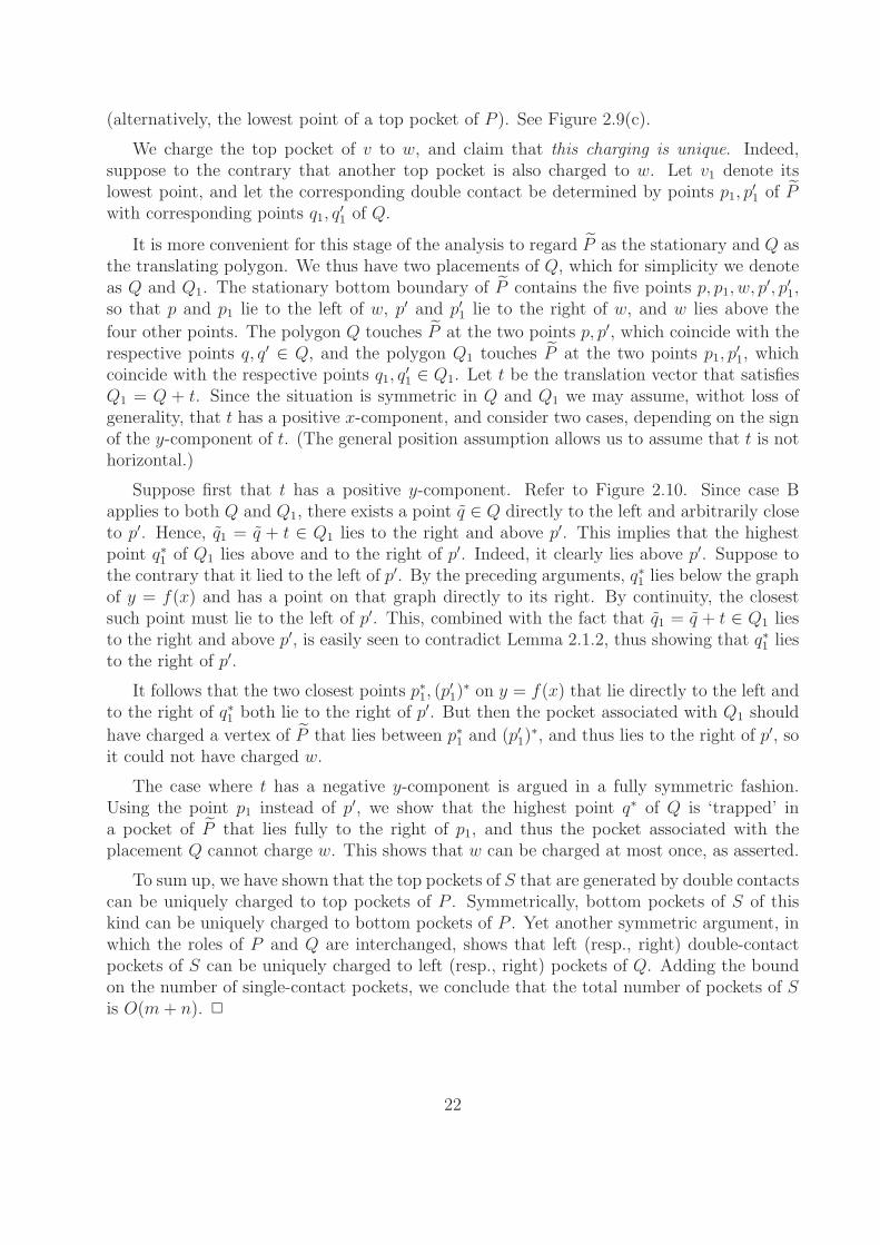
1 ∈ Q1. Let t be the translation vector that satisfiesQ1 = Q + t. Since the situation is symmetric in Q and Q1 we may assume, withot loss ofgenerality, that t has a positive x-component, and consider two cases, depending on the signof the y-component of t. (The general position assumption allows us to assume that t is nothorizontal.)

Suppose first that t has a positive y-component. Refer to Figure 2.10. Since case Bapplies to both Q and Q1, there exists a point q ∈ Q directly to the left and arbitrarily closeto p′. Hence, q1 = q + t ∈ Q1 lies to the right and above p′. This implies that the highestpoint q∗1 of Q1 lies above and to the right of p′. Indeed, it clearly lies above p′. Suppose tothe contrary that it lied to the left of p′. By the preceding arguments, q∗1 lies below the graphof y = f(x) and has a point on that graph directly to its right. By continuity, the closestsuch point must lie to the left of p′. This, combined with the fact that q1 = q + t ∈ Q1 liesto the right and above p′, is easily seen to contradict Lemma 2.1.2, thus showing that q∗1 liesto the right of p′.

It follows that the two closest points p∗1, (p′

1)∗ on y = f(x) that lie directly to the left and

to the right of q∗1 both lie to the right of p′. But then the pocket associated with Q1 should

have charged a vertex of P that lies between p∗1 and (p′1)∗, and thus lies to the right of p′, so

it could not have charged w.

The case where t has a negative y-component is argued in a fully symmetric fashion.Using the point p1 instead of p′, we show that the highest point q∗ of Q is ‘trapped’ ina pocket of P that lies fully to the right of p1, and thus the pocket associated with theplacement Q cannot charge w. This shows that w can be charged at most once, as asserted.

To sum up, we have shown that the top pockets of S that are generated by double contactscan be uniquely charged to top pockets of P . Symmetrically, bottom pockets of S of thiskind can be uniquely charged to bottom pockets of P . Yet another symmetric argument, inwhich the roles of P and Q are interchanged, shows that left (resp., right) double-contactpockets of S can be uniquely charged to left (resp., right) pockets of Q. Adding the boundon the number of single-contact pockets, we conclude that the total number of pockets of Sis O(m + n). 2

22

P

Q

Q1

p

p′

p1

p′1

w

q∗

q

q1

(p′1)∗p∗1 q∗1

Figure 2.10: Illustrating the proof that two top pockets of S of type B cannot both chargethe same pocket of P .

2.5 Minkowski Sum of Non-monotone Simple Polygons

The preceding machinery allows us to derive the main result of this paper:

Theorem 2.5.1 Let P be a simple polygon with m edges, which can be decomposed into ksimple subpolygons, all monotone in the x-direction, and let Q be a simple polygon with nedges, which can be decomposed into ℓ simple subpolygons, all monotone in the y-direction.Then the complexity of P ⊕ Q is O(kℓmnα(min{m,n})). The same holds if the x- andy-directions are replaced by two arbitrary directions.

Proof: Let P1, . . . , Pk be the k subpolygons in the decomposition of P , and let Q1, . . . , Qℓ

be the ℓ subpolygons in the decomposition of Q. Let mi denote the number of edges of Pi,for i = 1, . . . , k, and let ni denote the number of edges of Qi, for i = 1, . . . , ℓ. We have∑k

i=1mi = O(m) and

∑ℓ

i=1ni = O(n).

Put Sij := Pi ⊕ Qj, for i = 1, . . . , k and j = 1, . . . , ℓ. Clearly, S = P ⊕ Q =⋃

i,j Sij. ByTheorem 2.2.1, the complexity of Sij is O(minjα(min{mi, nj})). Hence, the total number ofedges of all the sums Sij is

O

((k∑

i=1

ℓ∑

j=1

minj

)α(min{m,n})

)= O(mnα(min{m,n})).

For each i and j, let T ∗

ij, B∗

ij, L∗

ij and R∗

ij denote the four connected portions of ∂Sij, asprovided by Theorem 2.3.1. Let X denote the collection of all the chains T ∗

ij and B∗

ij, and letY denote the collection of all the chains L∗

ij and R∗

ij. X is a set of 2kℓ x-monotone polygonalchains. The number of intersections of any pair of such chains is proportional to the numberof their edges, which is easily seen to imply that the complexity of the arrangement A(X) isO(kℓmnα(min{m,n})). Similarly, the complexity of A(Y ) is also O(kℓmnα(min{m,n})).

23

The complement of S is the union of some faces of the arrangement A(X ∪ Y ). Let Hdenote the collection of these faces. H contains one (the unique) unbounded face, and therest are bounded faces (‘holes’ of S). By the Combination Lemma for planar arrangements(see [24]), the overall complexity of all the faces of H (that is, the complexity of S) isproportional to the complexity of A(X) plus the complexity of A(Y ) plus |H|. Hence,Theorem 2.5.1 is an immediate consequence of the following lemma.

Lemma 2.5.2 The number of holes of P ⊕ Q is O(kℓmnα(min{m,n})).

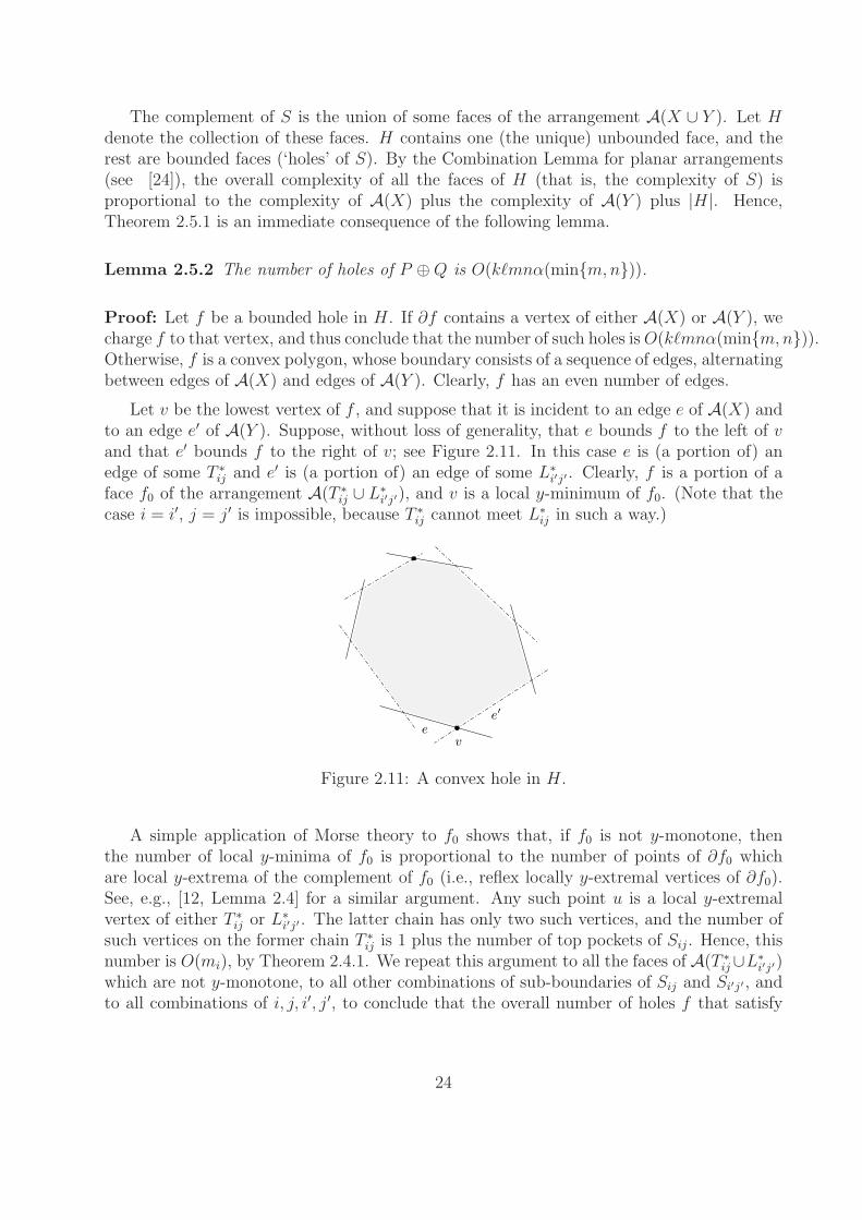
Proof: Let f be a bounded hole in H. If ∂f contains a vertex of either A(X) or A(Y ), wecharge f to that vertex, and thus conclude that the number of such holes is O(kℓmnα(min{m,n})).Otherwise, f is a convex polygon, whose boundary consists of a sequence of edges, alternatingbetween edges of A(X) and edges of A(Y ). Clearly, f has an even number of edges.

Let v be the lowest vertex of f , and suppose that it is incident to an edge e of A(X) andto an edge e′ of A(Y ). Suppose, without loss of generality, that e bounds f to the left of vand that e′ bounds f to the right of v; see Figure 2.11. In this case e is (a portion of) anedge of some T ∗

ij and e′ is (a portion of) an edge of some L∗

i′j′ . Clearly, f is a portion of aface f0 of the arrangement A(T ∗

ij ∪ L∗

i′j′), and v is a local y-minimum of f0. (Note that thecase i = i′, j = j′ is impossible, because T ∗

ij cannot meet L∗

ij in such a way.)

ve

e′

Figure 2.11: A convex hole in H.

A simple application of Morse theory to f0 shows that, if f0 is not y-monotone, thenthe number of local y-minima of f0 is proportional to the number of points of ∂f0 whichare local y-extrema of the complement of f0 (i.e., reflex locally y-extremal vertices of ∂f0).See, e.g., [12, Lemma 2.4] for a similar argument. Any such point u is a local y-extremalvertex of either T ∗

ij or L∗

i′j′ . The latter chain has only two such vertices, and the number ofsuch vertices on the former chain T ∗

ij is 1 plus the number of top pockets of Sij. Hence, thisnumber is O(mi), by Theorem 2.4.1. We repeat this argument to all the faces of A(T ∗

ij∪L∗

i′j′)which are not y-monotone, to all other combinations of sub-boundaries of Sij and Si′j′ , andto all combinations of i, j, i′, j′, to conclude that the overall number of holes f that satisfy

24

all the above conditions is

O

(∑

i,j,i′,j′

(mi + mi′)

)= O(mkℓ2) = O(kℓmn).

Suppose then that f0 is y-monotone. Then f0 has a unique y-minimal point (namely, v).If ∂f0 contains a vertex of either Sij or of Si′j′ then we charge v (uniquely) to such a vertex.Summing over all such faces f0 and over all i, j, i′, j′, we conclude that the number of holesf that fall into this subcase is

O

(∑

i,j,i′,j′

(minj + mi′nj′)α(min{m,n}))

= O(kℓmnα(min{m,n})).

We may thus assume that f0 is convex and bounded, and that the edges of its boundaryalternate between (portions of) edges of T ∗

ij and (portions of) edges of L∗

i′j′ . No edge of thetop boundary of f0 can belong to T ∗

ij, and thus the top boundary of f0 consists of a singleedge of L∗

i′j′ . Similarly, the left boundary of f0 consists of a single edge of T ∗

ij. We distinguishbetween two cases:

T

T

L

L

e2e1

v

T

Lf0

g0

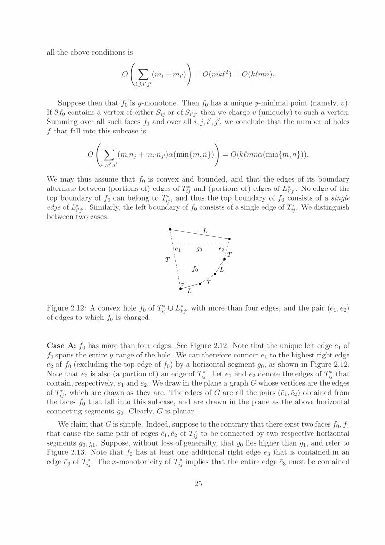
Figure 2.12: A convex hole f0 of T ∗

ij ∪ L∗

i′j′ with more than four edges, and the pair (e1, e2)of edges to which f0 is charged.

Case A: f0 has more than four edges. See Figure 2.12. Note that the unique left edge e1 off0 spans the entire y-range of the hole. We can therefore connect e1 to the highest right edgee2 of f0 (excluding the top edge of f0) by a horizontal segment g0, as shown in Figure 2.12.Note that e2 is also (a portion of) an edge of T ∗

ij. Let e1 and e2 denote the edges of T ∗

ij thatcontain, respectively, e1 and e2. We draw in the plane a graph G whose vertices are the edgesof T ∗

ij, which are drawn as they are. The edges of G are all the pairs (e1, e2) obtained fromthe faces f0 that fall into this subcase, and are drawn in the plane as the above horizontalconnecting segments g0. Clearly, G is planar.

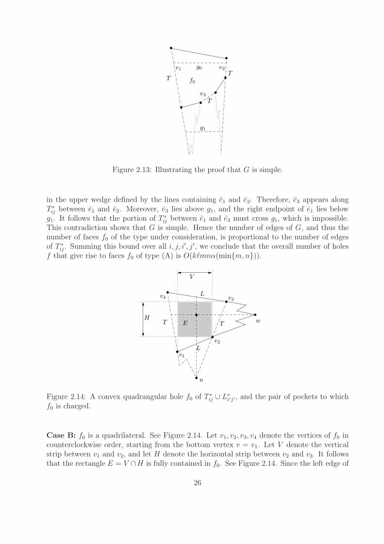
We claim that G is simple. Indeed, suppose to the contrary that there exist two faces f0, f1

that cause the same pair of edges e1, e2 of T ∗

ij to be connected by two respective horizontalsegments g0, g1. Suppose, without loss of generailty, that g0 lies higher than g1, and refer toFigure 2.13. Note that f0 has at least one additional right edge e3 that is contained in anedge e3 of T ∗

ij. The x-monotonicity of T ∗

ij implies that the entire edge e3 must be contained

25

T

T

e2e1

T

e3

g0

g1

f0

Figure 2.13: Illustrating the proof that G is simple.

in the upper wedge defined by the lines containing e1 and e2. Therefore, e3 appears alongT ∗

ij between e1 and e2. Moreover, e3 lies above g1, and the right endpoint of e1 lies belowg1. It follows that the portion of T ∗

ij between e1 and e3 must cross g1, which is impossible.This contradiction shows that G is simple. Hence the number of edges of G, and thus thenumber of faces f0 of the type under consideration, is proportional to the number of edgesof T ∗

ij. Summing this bound over all i, j, i′, j′, we conclude that the overall number of holesf that give rise to faces f0 of type (A) is O(kℓmnα(min{m,n})).

T

L

L

T

v1

v2

v3v4

H

V

E

u

w

Figure 2.14: A convex quadrangular hole f0 of T ∗

ij ∪ L∗

i′j′ , and the pair of pockets to whichf0 is charged.

Case B: f0 is a quadrilateral. See Figure 2.14. Let v1, v2, v3, v4 denote the vertices of f0 incounterclockwise order, starting from the bottom vertex v = v1. Let V denote the verticalstrip between v1 and v2, and let H denote the horizontal strip between v2 and v3. It followsthat the rectangle E = V ∩H is fully contained in f0. See Figure 2.14. Since the left edge of

26

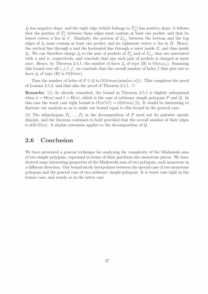
f0 has negative slope, and the right edge (which belongs to T ∗

ij) has positive slope, it followsthat the portion of T ∗

ij between these edges must contain at least one pocket, and that itslowest vertex u lies in V . Similarly, the portion of L∗

i′j′ between the bottom and the topedges of f0 must contain at least one pocket, and its rightmost vertex w lies in H. Hence,the vertical line through u and the horizontal line through w meet inside E, and thus insidef0. We can therefore charge f0 to the pair of pockets of T ∗

ij and of L∗

i′j′ that are associatedwith u and w, respectively, and conclude that any such pair of pockets is charged at mostonce. Hence, by Theorem 2.4.1, the number of faces f0 of type (B) is O(minj′). Summingthis bound over all i, j, i′, j′, we conclude that the overall number of holes f that give rise tofaces f0 of type (B) is O(kℓmn).

Thus the number of holes of P ⊕ Q is O(kℓmnα(min{m,n})). This completes the proofof Lemma 2.5.2, and thus also the proof of Theorem 2.5.1. 2

Remarks: (1) As already remarked, the bound in Theorem 2.5.1 is slightly suboptimalwhen k = Θ(m) and ℓ = Θ(n), which is the case of arbitrary simple polygons P and Q. Inthis case the worst case tight bound is O(m2n2) = O(kℓmn) [5]. It would be interesting tofinetune our analysis so as to make our bound equal to this bound in the general case.

(2) The subpolygons P1, . . . , Pk in the decomposition of P need not be pairwise openlydisjoint, and the theorem continues to hold provided that the overall number of their edgesis still O(m). A similar extension applies to the decomposition of Q.

2.6 Conclusion

We have presented a general technique for analyzing the complexity of the Minkowski sumof two simple polygons, expressed in terms of their partition into monotone pieces. We havederived some interesting properties of the Minkowski sum of two polygons, each monotone ina different direction. Our bound nicely interpolates between the special case of two monotonepolygons and the general case of two arbitrary simple polygons. It is worst case tight in theformer case, and nearly so in the latter case.

27

Bibliography

[1] P.K. Agarwal, E. Flato and D. Halperin, Polygon decomposition for efficient constructionof Minkowski sums, Comput. Geom. Theory Appl. 21:39–61, 2002.

[2] A. H. Barrera, Computing the Minkowski sum of monotone polygons, IEICE Trans. Inf.& Syst., E80-D (2):218–222, 1997.

[3] A. H. Barrera, Finding an O(n2 log n) algorithm is sometimes hard, In Proc. 8th Canad.Conf. Comput. Geom., pages 289–294. Carleton University Press, Ottawa, Canada, 1996.

[4] B. Chazelle, The polygon containment problem, In F. P. Preparata, editor, Compu-tational Geometry, volume 1 of Adv. Comput. Res., pages 1–33. JAI Press, London,England, 1983.

[5] M. de Berg, M. van Kreveld, M. Overmars and O. Schwarzkopf, Computational Geometry,Algorithms and Applications, 2nd Edition, Springer Verlag, Berlin-Heidelberg, 2000.

[6] M. de Berg and A. van der Stappen, On the fatness of minkowski sums, Technical ReportUUCS199939, Dept. of Computer Science, Utrecht University, 1999.

[7] G. Elber and M.S. Kim, editors, Special Issue of Computer Aided Design: Offsets, Sweepsand Minkowski Sums, 31, 1999.

[8] E. Flato, Robust and efficient construction of planar Minkowski sums, M.Sc. Dissertation,School of Computer Science, Tel Aviv University, 2000.

[9] E. Flato homepage. http://www.math.tau.ac.il/∼flato.

[10] E. Flato and D. Halperin, Robust and efficient construction of planar Minkowski sums,in Abstracts 16th European Workshop on Computational Geometry, Eilat, 2000, pages85–88.

[11] D. Halperin, J.C. Latombe, and R. H. Wilson, A general framework for assembly plan-ning: The motion space approach, Algorithmica, 26:577–601, 2000.

[12] D. Halperin and M. Sharir, Almost tight upper bounds for the single cell and zoneproblems in three dimensions, Discrete Comput. Geom. 14:385–410, 1995.

[13] S. Har-Peled, Multicolor combination lemmas, Comput. Geom. Theory Appl. 12:155–176, 1999.

28

[14] S. Har-Peled, T. M. Chan, B. Aronov, D. Halperin, and J. Snoeyink, The complexityof a single face of a Minkowski sum, In Proc. 7th Canad. Conf. Comput. Geom., pages91–96, 1995.

[15] E. Hartquist, J. Menon, K. Suresh, H. Voelcker, and J. Zagajac, A computing strategyfor applications involving offsets, sweeps, and Minkowski operations, Comput. AidedDesign, 31(4):175–183, 1999.

[16] A. Kaul, M. A. O’Connor, and V. Srinivasan, Computing Minkowski sums of regularpolygons, In Proc. 3rd Canad. Conf. Comput. Geom., pages 74–77, 1991.

[17] L. E. Kavraki, Computation of configuration space obstacles using the Fast FourierTransform, IEEE Trans. Robot. Autom., 11:408–413, 1995.

[18] K. Kedem, R. Livne, J. Pach and M. Sharir, On the union of Jordan regions andcollision-free translational motion amidst polygonal obstacles, Discrete Comput. Geom.1:59–71, 1986.

[19] J.C. Latombe, Robot Motion Planning, Kluwer Academic Publishers, Boston, 1991.

[20] R. Pollack, M. Sharir, and S. Sifrony, Separating two simple polygons by a sequence oftranslations, Discrete Comput. Geom., 3:123–136, 1988.

[21] G. Pustylnik and M. Sharir, The Minkowski sum of a simple polygon and a segment,Inform. Process. Lett. 85:179–184, 2003.

[22] G.D. Ramkumar, An algorithm to compute the Minkowski sum outer face of two simplepolygons, Proc. 12th Annu. ACM Sympos. Comput. Geom., 234-241, 1996.

[23] M. Sharir, Efficient algorithms for planning purely translational collision-free motionin two and three dimensions, Proc. IEEE Symp. on Robotics and Automation (1987),1326–1331.

[24] M. Sharir and P.K. Agarwal, Davenport-Schinzel Sequences and Their Geometric Ap-plications, Cambridge University Press, Cambridge-New York-Melbourne, 1995.

[25] G.T. Toussaint and H.A. ElGindy, Separation of two monotone polygons in linear time,Robotica 2:215–220, 1984.

[26] M. van Kreveld, Twelve computational geometry problems from cartographic general-ization, Manuscript. Presented at the Dagstuhl meeting on Computational Geometry,March, 1999.

29