minimizing communication in numerical linear algebra · minimizing communication in numerical...
TRANSCRIPT
Minimizing Communication in Numerical Linear
Algebra
Grey BallardJames DemmelOlga HoltzOded Schwartz
Electrical Engineering and Computer SciencesUniversity of California at Berkeley
Technical Report No. UCB/EECS-2011-15
http://www.eecs.berkeley.edu/Pubs/TechRpts/2011/EECS-2011-15.html
February 28, 2011

Copyright © 2011, by the author(s).All rights reserved.
Permission to make digital or hard copies of all or part of this work forpersonal or classroom use is granted without fee provided that copies arenot made or distributed for profit or commercial advantage and that copiesbear this notice and the full citation on the first page. To copy otherwise, torepublish, to post on servers or to redistribute to lists, requires prior specificpermission.

MINIMIZING COMMUNICATION IN NUMERICAL LINEARALGEBRA
GREY BALLARD ∗, JAMES DEMMEL † , OLGA HOLTZ ‡ , AND ODED SCHWARTZ §
Abstract. In 1981 Hong and Kung proved a lower bound on the amount of communication(amount of data moved between a small, fast memory and large, slow memory) needed to performdense, n-by-n matrix-multiplication using the conventional O(n3) algorithm, where the input ma-trices were too large to fit in the small, fast memory. In 2004 Irony, Toledo and Tiskin gave a newproof of this result and extended it to the parallel case (where communication means the amount ofdata moved between processors). In both cases the lower bound may be expressed as Ω(#arithmeticoperations /
√M), where M is the size of the fast memory (or local memory in the parallel case).
Here we generalize these results to a much wider variety of algorithms, including LU factorization,Cholesky factorization, LDLT factorization, QR factorization, Gram–Schmidt algorithm, algorithmsfor eigenvalues and singular values, i.e., essentially all direct methods of linear algebra.
The proof works for dense or sparse matrices, and for sequential or parallel algorithms. Inaddition to lower bounds on the amount of data moved (bandwidth-cost), we get lower bounds onthe number of messages required to move it (latency-cost).
We extend our lower bound technique to compositions of linear algebra operations (like computingpowers of a matrix), to decide whether it is enough to call a sequence of simpler optimal algorithms(like matrix multiplication) to minimize communication, or if we can do better. We give examplesof both. We also show how to extend our lower bounds to certain graph theoretic problems.
We point out recently designed algorithms that attain many of these lower bounds.
Key words. Linear algebra algorithms, bandwidth, latency, communication avoiding, lowerbound.
1. Introduction. Algorithms have two kinds of costs: arithmetic and commu-nication. By communication we mean either moving data between levels of a memoryhierarchy (in the sequential case) or over a network connecting processors (in theparallel case). There are two costs associated with communication: bandwidth-cost(proportional to the total number of words of data moved) and latency-cost (propor-tional to the number of messages in which these words are packed and sent). Forexample, we may model the cost of sending m words in a single message as α+ βm,where α is the latency (measured in seconds) and β is the reciprocal bandwidth (mea-sured in seconds per word). Depending on the technology, either latency or bandwidthcosts may be larger, often dominating the cost of arithmetic. So it is of interest tohave algorithms minimizing both bandwidth-cost and latency-cost.
In this paper we prove a general lower bound on the amount of data moved (i.e.,bandwidth-cost) by a general class of algorithms, including most dense and sparselinear algebra algorithms, as well as some graph theoretical algorithms. A similarmodel was discussed by Hong and Kung [HK81]. They show that to multiply two
∗Computer Science Department, University of California, Berkeley, CA 94720. Research sup-ported by Microsoft (Award #024263) and Intel (Award #024894) funding and by matching fundingby U.C. Discovery (Award #DIG07-10227). ([email protected]).†Mathematics Department and CS Division, University of California, Berkeley, CA 94720. This
material is based on work supported by U.S. Department of Energy grants under Grant NumbersDE-SC0003959, DE-SC0004938, and DE-FC02-06-ER25786, as well as Lawrence Berkeley NationalLaboratory Contract DE-AC02-05CH11231. ([email protected]).‡Departments of Mathematics, University of California, Berkeley and Technische Universitat
Berlin. O. Holtz acknowledges support of the Sofja Kovalevskaja program of Alexander von Hum-boldt Foundation. ([email protected]).§ The Weizmann Institute of Science, Rehovot 76100, Israel. This work was done while at the De-
partments of Mathematics, Technische Universitat Berlin, and while visiting University of California,Berkeley. ([email protected]).
1
2 BALLARD, DEMMEL, HOLTZ, AND SCHWARTZ
dense n-by-n matrices, using the conventional Θ(n3) algorithm, on a machine with alarge slow memory (in which the matrices initially reside) and a small fast memoryof size M (too small to store the matrices, but arithmetic may only be done on datain fast memory), Ω(n3/
√M) words of data must be moved between fast and slow
memory. This lower bound is attained by a variety of “blocked” algorithms. Thislower bound may also be expressed as Ω(#arithmetic operations /
√M) 1.
This result was proven differently by Irony, Toledo and Tiskin [ITT04] and gen-eralized to the parallel case, where P processors multiply two n-by-n matrices. Inthe “memory-scalable” case, where each processor stores the minimal M = O(n2/P )words of data, they obtain the lower bound:Ω(#arithmetic operations per processor /
√memory per processor) = Ω( n3/P√
n2/P) =
Ω( n2√
P), which is attained by Cannon’s algorithm [Can69] [Dem96, Lecture 11]. The
paper [ITT04] also considers the so-called “3D” case, which does less communicationby replicating the matrices and using O(P 1/3) times as much memory as the minimalpossible.
Here we begin with the proof in [ITT04], which starts with the sum Cij =∑
k Aik ·Bkj , and uses a geometric argument on the lattice of indices (i, j, k) to bound thenumber of updates Cij := Cij + Aik · Bkj that can be performed when a subset ofmatrix entries are in fast memory. This proof generalizes in a number of ways: inparticular it does not depend on the matrices being dense, or the output being distinctfrom the input. These observations let us state and prove a general Theorem 2.2 inSection 2, that a lower bound on the number of words moved into or out of a fast orlocal memory of size M is Ω(#arithmetic operations /
√M ). This applies to both
the sequential case (where M is a fast memory) and the parallel case (where M is eachprocessor’s local memory); in the parallel case further assumptions about whether thealgorithm is memory or load balanced (to estimate the effective M and #arithmeticoperations) are needed to get a lower bound on the overall algorithm.
Corollary 2.3 of Theorem 2.2 provides a simple lower bound on latency-cost (justthe lower bound on bandwidth-cost divided by the largest possible message size,namely the memory size M). Both bandwidth-cost and latency-cost lower boundsapply straightforwardly to a nested memory hierarchy with more than two layers,bounding from below the communication between any adjacent layers in the hierar-chy [Sav95, BDHS10a].
In Section 3, we present simple corollaries applying Theorem 2.2 to conventional(non-Strassen-like) implementations of matrix multiplication and other BLAS opera-tions [BDD+02, BDD+01] (dense or sparse), LU factorization, Cholesky factorizationand LDLT factorization, where D is either real diagonal matrix, or block-diagonalmatrix, i.e., Bunch-Kaufman [BK77] type factorization. These factorizations mayalso be dense or sparse, with any kind of pivoting, and be exact or “incomplete”, e.g.,ILU [Saa96] (for dense matrices some of these results can be also obtained by suitablereductions from [HK81] or [ITT04], and we point these out). We also introduce a tech-nique to extend these lower bounds to cases like computing ‖A ·B‖F , so the output isa single scalar, and where each A(i, j) and B(j, k) is given by an explicit formula, sothere are no inputs to read from memory (we will require that each explicit formula
1The sequential communication model used here is sometimes called the two-level I/O modelor disk access machine (DAM) model (see [AV88], [BBF+07], [CR06]). Our model follows that of[HK81] and [ITT04] in that it assumes the block-transfer size is one word of data (B = 1 in thecommon notation).

MINIMIZING COMMUNICATION IN LINEAR ALGEBRA 3
is evaluated at most once).Section 4 considers lower bounds for algorithms that involve orthogonal factor-
izations. This class includes the QR factorization, the standard algorithms for eigen-values and eigenvectors, and the singular value decomposition (SVD). After dealingwith the easier case of Gram-Schmidt in Section 4.1, Section 4.2 considers the hardercase of algorithms that apply sequences of orthogonal transformations. For reasonsexplained there, the counting techniques of [HK81] and [ITT04] do not directly ap-ply, so we need a different but related lower bound argument. Our proofs requiresome technical assumptions that we conjecture could be removed. Finally, Section 4.3extends the lower bounds to eigenvalue and singular value problems.
Section 5 shows how to extend our lower bounds to more general computationswhere we compose a sequence of simpler linear algebra operations (like matrix multi-plication, LU decomposition, etc.), so the outputs of one operation may be inputs tolater ones. If these intermediate results do not need to be saved in slow memory, or ifsome inputs are given by formulas (like A(i, j) = 1/(i+ j)) and so do not need to befetched from memory, or if the final output is just a scalar (the norm or determinantof a matrix), then it is natural to ask whether there is a better algorithm than justusing optimized versions of each operation in the sequence. We give examples wherethis simple approach is optimal and when it is not. We also exploit the natural cor-respondence between matrices and graphs to derive communication lower bounds forcertain graph algorithms, like All-Pairs-Shortest-Path.
Finally, Section 6 discusses attainability of these lower bounds, and open prob-lems. Briefly, in the dense case all the lower bounds are attainable (in the parallelcase, this is modulo polylogP factors, and assuming the minimal O(n2/P ) storage perprocessor); see Tables 6.1 and 6.2 (some of these algorithms are also pointed out insections 3 and 4.2). The optimal algorithms for square matrix multiplication are wellknown, as mentioned above. Optimal algorithms for dense LU, Cholesky, QR, eigen-value problems and the SVD are more recent and not part of standard libraries likeLAPACK [ABB+92] and ScaLAPACK [BCC+97]. Several of these references describeprototypes of the new algorithms that attain large speedups over standard libraries.Beyond the BLAS, only in the case of Cholesky do we know of a sequential algorithmthat does as few flops as the conventional algorithm (modulo lower order terms) aswell as achieving both minimal bandwidth-cost and latency-cost across arbitrary lev-els of memory hierarchy. Beyond Cholesky [BDHS10a, DDGP10] and the BLAS, nooptimal algorithm is known for architectures mixing parallelism and multiple memoryhierarchies, i.e., most real architectures (but some lower bounds for specific architec-ture/algorithm combinations do exist, see for example [Saa86]). “3D” algorithms, thatuse multiple copies of the data in order to communicate less than “2D” algorithmsusing minimal total memory, were obtained in [IT02, Ash91, Ash93, SD11], and arediscussed in Section 6. Communication optimal algorithms for sparse matrices areknown only for sparse Cholesky [DDGP10]. For highly rectangular dense matrices(e.g., matrix-vector multiplication) or for sufficiently sparse matrices, our new lowerbound is sometimes lower than the trivial lower bound (#inputs + #outputs) andtherefore not always attainable.
2. First Lower Bound. We first define our model of computation formally, andillustrate it on the simplest case of dense matrix multiplication.
We work with n × n matrices, so we define V = 1, 2, ...n to be the index setfor the rows and columns. Let Sa ⊆ V × V be the subset of entries of the indices ofthe input matrix A that are read by the algorithm (e.g., the indices of the non-zeros

4 BALLARD, DEMMEL, HOLTZ, AND SCHWARTZ
entries of a sparse matrix). Let a : Sa 7→ M be a mapping from the matrix entries tolocations in memory (on a parallel machineM refers to a location in some processor’smemory; the processor number is implicit). The map is one-to-one. Similarly defineSb, Sc and b(·, ·), c(·, ·) for the matrices B and C. Note that the ranges of a, b and care not necessarily disjoint. The value of a memory location l is denoted by Mem(l).
Now let fij and gijk be “nontrivial” functions in a sense we make clear below.The computation we want to perform is for all (i, j) ∈ Sc:
Mem(c(i, j)) = fij(gijk(Mem(a(i, k)),Mem(b(k, j))) for k ∈ Sij , any other arguments)(2.1)
Here fij depends nontrivially on its arguments gijk(·, ·) which in turn depend non-trivially on their arguments Mem(a(i, k)) and Mem(b(k, j)), in the following sense:we need at least one word of space to compute fij (which may or may not beMem(c(i, j))) to act as “accumulator” of the value of fij , and we need the valuesMem(a(i, k)) and Mem(b(k, j)) in fast memory before evaluating gijk. Note alsothat we may not know until after the computation what SC , fij , Sij , gijk or “anyother arguments” were, since they may be determined on the fly (e.g., pivot order).
Now we illustrate the model in Equation (2.1) by applying it to sequential densen-by-n matrix multiplication C = A ·B, where A, B and C are stored column-wise inmemory: We take Sc as all pairs (i, j) with 0 ≤ i, j < n with C(i, j) stored in locationc(i, j) = i+j ·n. A(i, k) is analogously stored at location a(i, k) = i+k ·n and B(k, j)is stored at location b(k, j) = k + j · n. The set Sij = 0, 1, ..., n − 1 for all (i, j).Operation gijk is scalar multiplication, and fij computes the sum of its n arguments.
The question is how many slow memory references are required to perform thiscomputation, when all we are allowed to do is compute the gijk in a different order,and compute and store the fij is a different order. This appears to restrict possiblereorderings to those where fij is computed correctly, since we are not assuming it isan associative or commutative function, or those reorderings that avoid races becausesome c(i, j) may be used later as inputs. But there is no need for such restrictions: thelower bound applies to all reorderings, correct or incorrect, yielding the same boundin both cases.
Using only structural information, e.g., about the sparsity patterns of the ma-trices, we can sometimes deduce that the computed result fij(·) is exactly zero, topossibly avoid a memory reference to store the result at c(i, j). Section 3.2.1 discussesthis possibility more carefully, and shows how to carefully count operations to preservethe validity of our lower bounds.
The argument, following [ITT04], is:• Break the stream of instructions executed into segments, where each segment
contains exactly M load and store instructions (i.e., that cause communica-tion), where M is the fast (or local) memory size.
• Bound from above the number of evaluations of functions gijk that can beperformed during any segment, calling this upper bound F .
• Bound from below the number of (complete) segments by the total numberof evaluations of gijk (call it G) divided by F , i.e., bG/F c.
• Bound from below the total number of loads and stores, by M (load/storesper segment) times the minimum number of complete segments, bG/F c, soit is at least M · bG/F c.
Now we compute the upper bound F using a geometric theorem of Loomis and Whit-
MINIMIZING COMMUNICATION IN LINEAR ALGEBRA 5
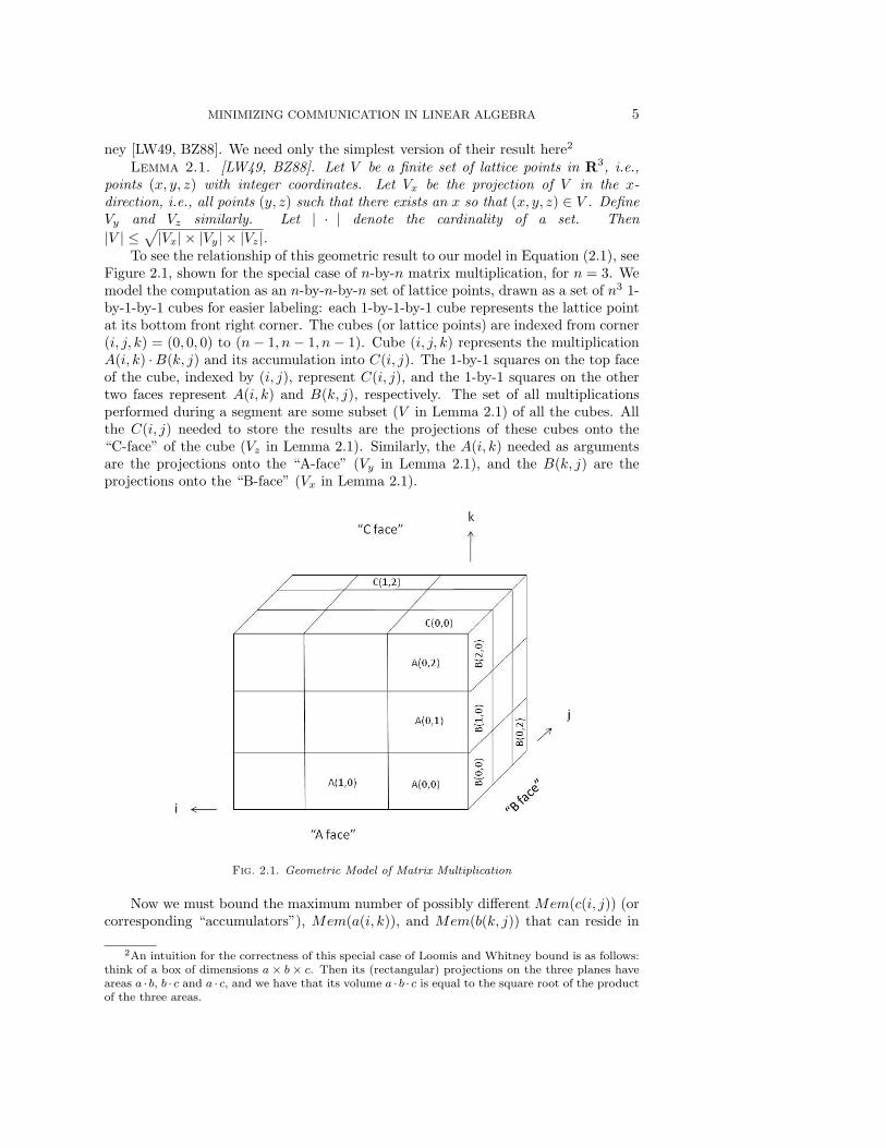
ney [LW49, BZ88]. We need only the simplest version of their result here2
Lemma 2.1. [LW49, BZ88]. Let V be a finite set of lattice points in R3, i.e.,points (x, y, z) with integer coordinates. Let Vx be the projection of V in the x-direction, i.e., all points (y, z) such that there exists an x so that (x, y, z) ∈ V . DefineVy and Vz similarly. Let | · | denote the cardinality of a set. Then|V | ≤
√|Vx| × |Vy| × |Vz|.
To see the relationship of this geometric result to our model in Equation (2.1), seeFigure 2.1, shown for the special case of n-by-n matrix multiplication, for n = 3. Wemodel the computation as an n-by-n-by-n set of lattice points, drawn as a set of n3 1-by-1-by-1 cubes for easier labeling: each 1-by-1-by-1 cube represents the lattice pointat its bottom front right corner. The cubes (or lattice points) are indexed from corner(i, j, k) = (0, 0, 0) to (n− 1, n− 1, n− 1). Cube (i, j, k) represents the multiplicationA(i, k) ·B(k, j) and its accumulation into C(i, j). The 1-by-1 squares on the top faceof the cube, indexed by (i, j), represent C(i, j), and the 1-by-1 squares on the othertwo faces represent A(i, k) and B(k, j), respectively. The set of all multiplicationsperformed during a segment are some subset (V in Lemma 2.1) of all the cubes. Allthe C(i, j) needed to store the results are the projections of these cubes onto the“C-face” of the cube (Vz in Lemma 2.1). Similarly, the A(i, k) needed as argumentsare the projections onto the “A-face” (Vy in Lemma 2.1), and the B(k, j) are theprojections onto the “B-face” (Vx in Lemma 2.1).
Fig. 2.1. Geometric Model of Matrix Multiplication
Now we must bound the maximum number of possibly different Mem(c(i, j)) (orcorresponding “accumulators”), Mem(a(i, k)), and Mem(b(k, j)) that can reside in
2An intuition for the correctness of this special case of Loomis and Whitney bound is as follows:think of a box of dimensions a× b× c. Then its (rectangular) projections on the three planes haveareas a · b, b · c and a · c, and we have that its volume a · b · c is equal to the square root of the productof the three areas.

6 BALLARD, DEMMEL, HOLTZ, AND SCHWARTZ
fast memory during a segment. Since we want to accommodate the most general casewhere input and output arguments can overlap, we need to use a more complicatedmodel than in [ITT04], where no such overlap was possible. To this end, we considereach input or output operand of (2.1) that appears in fast memory during a segmentof M slow memory operations. It may be that an operand appears in fast memoryfor a while, disappears, and reappears, possibly several times (we assume there is atmost one copy at a time in the sequential model and at most one for each processorin the parallel model; this assumption is consistent with obtaining a lower bound).For each period of continuous existence of an operand in fast memory, we label itsRoot (how it came to be in fast memory) and its Destination (what happens whenit disappears):
• Root R1: The operand was already in fast memory at the beginning ofthe segment, and/or read from slow memory. There are at most 2M suchoperands altogether, because the fast memory has size M , and because asegment contains at most M reads from slow memory.
• Root R2: The operand is computed (created) during the segment. Withoutmore information, there is no bound on the number of such operands.
• Destination D1: An operand is left in fast memory at the end of the segment(so that it is available at the beginning of the next one), and/or written to slowmemory. There are at most 2M such operands altogether, again because thefast memory has size M , and because a segment contains at most M writesto slow memory.
• Destination D2: An operand is neither left in fast memory nor written toslow memory, but simply discarded. Again, without more information, thereis no bound on the number of such operands.
We may correspondingly label each period of continuous existence of any operandin fast memory during one segment by one of four possible labels Ri/Dj, indicatingthe Root and Destination of the operand at the beginning and end of the period.Based on the above description, the total number of operands of all types exceptR2/D2 is bounded by 4M (the maximum number of R1 operands plus the numberof D1 operands, an upper bound) 3. The R2/D2 operands, those created duringthe segment and then discarded without causing any slow memory traffic, cannot bebounded without further information. For our simplest model, adequate for matrixmultiplication, LU decomposition, etc., we have no R2/D2 arguments; they reappearwhen we analyze the QR decomposition in Section 4.2.
Using the set of lattice points (i, j, k) to represent each function evaluationgijk(Mem(a(i, k)),Mem(b(k, j))), and assuming there are no R2/D2 arguments, thenwe can use Lemma 2.1 to bound F : We let V be the set of indices (i, j, k) of the gijk
operations, Vz be the set of indices (i, j) of their destinations c(i, j) with |Vz| ≤ 4M ,Vy be the set of indices (i, k) of their arguments a(i, k) with |Vy| ≤ 4M , and Vx bethe set of indices (j, k) of their arguments b(j, k) with |Vx| ≤ 4M . Then Lemma 2.1bounds F = |V | ≤
√|Vx| × |Vy| × |Vz| ≤
√(4M)3. Therefore the total number of
loads and stores is bounded by MbGF c = Mb G√
(4M)3c ≥ G
8√
M−M . This proves the
first lower bound:Theorem 2.2. In the notation defined above, and in particular assuming there
are no R2/D2 arguments (created and discarded without causing memory traffic) thenumber of loads and stores needed to evaluate (2.1) is at least G
8√
M−M .
3More careful but complicated accounting can reduce this upper bound to 3M .
MINIMIZING COMMUNICATION IN LINEAR ALGEBRA 7
We may also write this as Ω(#arithmetic operations /√M) understanding that
we only count arithmetic operations required to evaluate the gijk for (i, j) ∈ SC andk ∈ Sij . We note that a more careful, problem-dependent analysis that depends onhow much the three arguments can overlap, may sometimes increase the lower boundby a factor of as much as 8, but for simplicity we omit this.
This lower bound is not always attainable, even for dense matrix multiplication: Ifthe matrices are so small that they all fit in fast memory simultaneously, so 3n2 ≤M ,then the number of loads and stores may be just 3n2, which can be much larger thann3/√M . So a more refined lower bound is max(G/(8
√M)−M,#inputs + #outputs).
We generally omit this detail from statements of later corollaries.Theorem 2.2 is a lower bound on bandwidth-cost, the total number of words
communicated. But it immediately provides a lower bound on latency-cost as well,the minimum number of messages that need to be sent, where each message maycontain many words.
Corollary 2.3. In the notation defined above, the number of messages neededto evaluate (2.1) is at least G/(8M3/2)− 1 = #evaluations of gijk/(8M3/2)− 1.
The proof is simply that the largest possible message size is the fast (or local)memory size M , so we divide the lower bound from Theorem 1 by M .
On a parallel computer it is possible for a processor to pack M words into a singlemessage to be sent to a different processor. But on a sequential computer the words tobe sent in a single message must generally be located in contiguous memory locations,which depends on the data structures used. This model is appropriate to capture thebehavior of real hardware, e.g., cache lines, memory prefetching, disk accesses, etc.This requirement means that to attain the latency-cost lower bound on a sequentialcomputer, rather different matrix data structures may be required than row-major orcolumn-major [BDHS10a, FLPR99, EGJK04, AGW01, AP00].
Finally, we note that real computers typically don’t have just one level of memoryhierarchy, but many, each with its own underlying bandwidth and latency costs. Soit is of interest to minimize all communication, between every pair of adjacent levelsof the memory hierarchy. As has been noted before [Sav95, BDHS10a], when thememory hierarchy levels are nested (the L2 cache stores a subset of L3 cache, etc.)we can apply lower bounds like ours at every level in the hierarchy.
3. Consequences for BLAS, LU , Cholesky, and LDLT . We now show howTheorem 2.2 applies to a variety of conventional algorithms from numerical linearalgebra, by which we mean algorithms that would cost O(n3) arithmetic operationswhen applied to dense n-by-n matrices, as opposed to Strassen-like algorithms.
It is natural to ask whether algorithms exist that attain these lower bounds. Wepoint out cases where we know such algorithms exist, which are therefore optimal inthe sense of minimizing communication. In the case of dense matrices, many optimalalgorithms are known, though not yet in all cases. In the case of sparse matrices,little seems to be known.
3.1. Matrix Multiplication and the BLAS. We begin with matrix multipli-cation, on which our model in Equation (2.1) is based:
Corollary 3.1. G/(8√M) −M is the bandwidth-cost lower bound for multi-
plying explicitly stored matrices C = A · B on a sequential machine, where G is thenumber of multiplications performed in evaluating all the Cij =
∑k Aik ·Bkj, and M
is the fast memory size. In the special case of multiplying a dense n-by-r matrix timesa dense r-by-m matrix, this lower bound is n · r ·m/
√8M −M .

8 BALLARD, DEMMEL, HOLTZ, AND SCHWARTZ
This nearly reproduces a result in [ITT04] for the case of two distinct, densematrices, whereas we need no such assumptions; their bound is
√8 times larger than
ours, but as stated before our bound could be improved by specializing it to thiscase. We note that this result could have been stated for sparse A and B in [HK81]:Combine their Theorem 6.1 (their Ω(|V |) is the number of multiplications) with theirLemma 6.1 (whose proof does not require A and B to be dense).
As noted in the previous section, an independent lower bound on the bandwidth-cost is simply the total number of inputs that need to be read plus the number ofoutputs that need to be written. But counting the number of inputs is not as simple ascounting the number of nonzero entries of A and B: if A and B are sparse, and columni of A is filled with zeros only, then row i of B need not be loaded at all, since C doesnot depend on it. An algorithm that nevertheless loads row i of B will still satisfy thelower bound. And an algorithm that loads and multiplies by explicitly stored zeroentries of A or B will also satisfy the lower bound. Multiplications that involve suchzero entries is an optimization sometimes used in practice (e.g., [VDY05]).
When A and B are dense and distinct, there are well-known algorithms mentionedin the Introduction that (nearly) attain the combined lower bound
Ω(max(n·r·m/√M,#inputs+#outputs)) = Ω(max(n·r·m/
√M,n·r+r·m+n·m)) ,
see [ITT04] for a more complete discussion. Attaining the corresponding latency-cost lower bound of Corollary 2.3 requires a different data structure than the usualrow-major or column-major orders, so that words to be sent in a single message arecontiguous in memory, and is variously referred to as recursive block storage or storageusing space filling curves, see [FLPR99, EGJK04, BDHS10a] for discussion. Some ofthese algorithms also minimize bandwidth-cost and latency-cost for arbitrarily manylevels of memory hierarchy. Little seems to be known about the attainability of thislower bound for general sparse matrices.
Now we consider the parallel case, with P processors. Let nnz(A) be the numberof nonzero entries of A; then NNZ = nnz(A) + nnz(B) + nnz(C) is a lower bound onthe total memory required to store the inputs and outputs. We need to make someassumption about how this data is spread across processors (each of which has itsown memory), since if A, B and C were all stored in one processor, and all arithmeticdone there (i.e., no parallelism at all), then no communication would be needed. Itis enough to assume either that (1) the memory is balanced among the processors, orthat (2) the arithmetic is balanced. In the first case, each processor stores an equalshare NNZ/P of the data (and perhaps at most o(NNZ/P ) more words). Then atleast one processor must perform at least G/P multiplications, where G is the totalnumber of multiplications (they can’t all be below average); the theorem below willapply to the communication done by this processor. In the second case, each processordoes G/P multiplications (give or take o(G/P )). Then at least one processor storesat most NNZ/P words (they can’t all be above average); the theorem below will applyto the communication done by this processor. Combining all this with Theorem 2.2yields4
Corollary 3.2. Suppose we have a parallel algorithm on P processors for mul-tiplying matrices C = A · B that is memory-balanced in the sense described above.
4We present the conclusions for the parallel model in asymptotic notation. One could instead
assume that each processor had memory of size M = µ · n2
Pfor some constant µ, and obtain the
hidden constant of the lower bounds as a function of µ, as done in [ITT04].
MINIMIZING COMMUNICATION IN LINEAR ALGEBRA 9
Then at least one processor must communicate Ω(G/√P · NNZ −NNZ/P
)words,
where G is the number of multiplications Aij · Bkj performed. In the special case of
dense n-by-n matrices, this lower bound is Ω(n2/√P)
.There are again well-known algorithms that attain the bandwidth-cost and latency-
cost lower bounds in the dense case, but not in the sparse case.We next extend Theorem 2.2 beyond matrix multiplication. The simplest exten-
sion is to the so-called BLAS3 (Level-3 Basic Linear Algebra Subroutines [BDD+01,BDD+02]), which include related operations like multiplication by (conjugate) trans-posed matrices, by triangular matrices and by symmetric (or Hermitian) matrices.The last two corollaries apply to these operations without change (in the case ofAT · A we use the fact that Theorem 2.2 makes no assumptions about the matricesbeing multiplied not overlapping).
More interesting is the BLAS3 operation TRSM, computing C = A−1B where Ais triangular. The inner loop of the algorithm (when A is upper triangular) is
Cij = (Bij −n∑
k=i+1
Aik · Ckj)/Aii (3.1)
which can be executed in any order with respect to j, but only in decreasing orderwith respect to i. None of this matters for the lower bound, since equation (3.1)still matches Equation (2.1), so the lower bounds apply. To see this, we make thecorrespondences that Cij is stored at location c(i, j) = b(i, j), Aik is stored at locationa(i, k), gijk multiplies Aik ·Ckj , and fij performs the indicated sum, subtracts it fromBij , and divides by Aii. The fact that output Cij coincides with the input (so it couldbe of type R2/D1) does not matter. Sequential algorithms that attain these boundsfor dense matrices, for arbitrarily many levels of memory hierarchy, are discussed in[BDHS10a].
We note that our lower bound also applies to the so-called Level 2 BLAS (likematrix-vector multiplication) and Level 1 BLAS (like dot products), but the largerlower bound #inputs + #outputs is attainable.
3.2. LU factorization. Independent of sparsity and pivot order, the formulasdescribing LU factorization are as follows, with the understanding the summationsmay be over some subset of the indices k in the sparse case, and pivoting has alreadybeen incorporated in the interpretation of the indices i, j and k.
Lij = (Aij −∑k<j
Lik · Ukj)/Ujj for i > j (3.2)
Uij = Aij −∑k<i
Lik · Ukj for i ≤ j
We see that these formulas correspond to our model in Equation (2.1), with a(i, j) =b(i, j) = c(i, j) (since L and U are both inputs and outputs, overwriting A), gijk
identified with multiplying Lik ·Ukj , and fij summing the operands, subtracting fromAij , and possibly dividing by Ujj . The fact that the “outputs” Lij and Uij coincidewith the inputs (so they could be of type R2/D1) does not matter, as before.
We discuss the more subtle question of incomplete LU (ILU) in the next section.A sequential dense LU algorithm that attains this bandwidth-cost lower bound
is given by [Tol97], although it does not always attain the latency-cost lower bound
10 BALLARD, DEMMEL, HOLTZ, AND SCHWARTZ
[DGHL08a]. The conventional parallel dense LU algorithm implemented in ScaLA-PACK [BCC+97] attains the bandwidth-cost lower bound (modulo an O(logP ) fac-tor), but not the latency-cost lower bound. A parallel algorithm that attains bothlower bounds (again modulo a factor O(logP )) is given in [DGX08], where significantspeedups are reported. Interestingly, it does not seem possible to attain both lowerbounds and retain conventional partial pivoting; a different (but still stable) kind ofpivoting is required. We also know of no dense sequential LU algorithm that mini-mizes bandwidth-cost and latency-cost across multiple levels of a memory hierarchy(unlike Cholesky). There is an elementary reduction proof that dense LU factoriza-tion is “as hard as dense matrix multiplication” [DGHL08a], but it does not addresssparse or incomplete LU, as does our approach.
3.2.1. How to count operations gijk carefully. Once an algorithm has com-pleted running, the type Ri/Dj of each argument is well-defined based on the actualsequence of operations performed, but it may be hard to tell by inspecting the sourcecode of the algorithm (or other high level description) which operations to count asgijk in the total G used in the statement of Theorem 2.2.
A sufficient, but not necessary, condition for counting gijk, is as follows: If a(i, k)and b(k, j) are originally stored in memory and never modified, then they can only beR1 and not R2; they are always D2. If c(i, j) is only computed once and eventuallystored to memory, it can only be D1 and not D2; it could be either R1 or R2, dependingon the segment. In this situation, which covers the BLAS, LU and other “complete”factorizations, there are clearly no R2/D2 arguments, and we count all multiplications.(Arguments of type R2/D2 appear later in Section 4, and require different countingtechniques.)
In other situations, where it may be difficult to tell which gijk to count, it maybe easier to identify a subset of them that are recognized as satisfying a conditionas in the last paragraph, and just count this subset. This may undercount the totalnumber G of gijk, but still provides a valid lower bound.
We give some examples to illustrate the counting process.Example 1. Consider incomplete LU (ILU) factorization [Saa96], where some entriesof L and U are omitted in order to speedup the computation. In particular, considerthreshold based ILU, which computes a possible nonzero entry Lij or Uij and comparesit to a threshold, storing it only if it is larger than the threshold and discarding itotherwise. Which multiplications Lik · Ukj do we count? We may underestimatethe total number G of multiplications by simply not counting any multiplicationsthat lead to a value of Lij or Uij that is discarded. Thus we see that analogues ofCorollaries 3.1 and 3.2 apply to ILU as well (and later to incomplete Cholesky, etc.).Example 2. Using only structural information, e.g., about the sparsity patterns ofthe underlying matrices, it is sometimes possible to deduce that the computed resultfij(·) is exactly zero, and so to possibly avoid a memory reference to location c(i, j)to store the result. This may either be because the values gijk(·) being accumulatedto compute fij are all identically zero, or, more interestingly, because it is possible toprove there is exact cancellation (independent of the values of the nonzero argumentsMem(a(i, k)) and Mem(b(k, j))). Here is an example.
Consider a matrix A that is nonzero in its first r rows and columns, and possiblyin the trailing (n− 2r)-by-(n− 2r) submatrix; call this submatrix A′. First supposeA′ = 0, so that A has rank at most 2r, and that pivots are chosen along the diagonal.It is easy to see that the first 2r− 1 steps of Gaussian elimination will generically fillin the entire matrix with nonzeros, but that step 2r will cause cancellation to zero
MINIMIZING COMMUNICATION IN LINEAR ALGEBRA 11
(in exact arithmetic) in all entries of A′. If A′ starts as a nonzero sparse matrix, thenthis cancellation will not be to zero but to the sparse LU factorization of A′ alone.So one can imagine an algorithm that may or may not recognize this opportunity toavoid work in some or all of the entries of A′. To accommodate all these possibilities,we could, as above, only count those multiplications gijk (3.2) that contribute to aresult Lij or Uij that is stored in memory, possibly underestimating G.
Analogous examples exist for factorizations discussed later, such as LDLT andQR.
As a short-hand, in Section 4.2 we will sometimes refer to a matrix entry as beingtreated as nonzero if the algorithm assumes that its value could be nonzero in decidingwhether to bother performing gijk. Thus an algorithm for dense matrices treats allentries as nonzero, even if the input matrix is sparse, whereas a sparse factorizationalgorithm would not.Example 3. Consider n-by-n boolean matrix multiplication C = A · B, where thefirst column of A and first row of B consist entirely of ones. Then one can deducethat C consists entirely of ones without reading any other columns of A or rows ofB. Thus an algorithm could perform as few as n2 gijk evaluations (boolean and’s)along with 2n + n2 loads and stores, or as many as n3 gijk evaluations along withΩ(n3/
√M) loads and stores, depending on the algorithm and input matrices. Either
way, the theorem applies.Example 4. It is possible to have no R2/D2 arguments, even if a matrix entry,say a(i, k), requires no memory accesses, as long as it is processed in a way like thefollowing: In segment 1, a(i, j) is computed by a formula, and left in fast memory,so it is R2/D1 in segment 1. In segment 2, a(i, j) starts in fast memory at the startof the segment, and is left there at the end, so it is R1/D1 in segment 2. Finally, insegment 3, a(i, j) starts in fast memory at the start of the segment, and discardedbefore the end, so it is R1/D2 in segment 3. To see that we could potentially havemany such arguments, consider the realistic problem of computing the determinant ofa matrix A from its LU decomposition, where each entry of A is given by a formula,and we discard the LU decomposition after computing the product
∏i U(i, i). We give
a more systematic way of counting gijk accurately for examples like this in Section 5.
3.3. Cholesky Factorization. Now we consider Cholesky factorization. In-dependent of sparsity and (diagonal) pivot order, the formulas describing Choleskyfactorization are as follows, with the understanding the summations may be over somesubset of the indices k in the sparse case, and pivoting has already been incorporatedin the interpretation of the indices i, j and k.
Ljj = (Ajj −∑k<j
L2jk)1/2 (3.3)
Lij = (Aij −∑k<j
Lik · Ljk)/Ljj for i > j
It is easy to see that these formulas correspond to our model in Equation (2.1), withgijk identified with multiplying Lik ·Ljk. As before, the fact that the “outputs” Lij canoverwrite the inputs does not matter, and the subtraction from Aij , division by Lii,and square root are all accommodated by Equation (2.1). As before, these formulasare general enough to accommodate incomplete Cholesky (IC) factorization [Saa96].
Dense algorithms that attain these lower bounds are discussed in [BDHS10a],both parallel and sequential, including analyzing one that minimizes bandwidth-cost
12 BALLARD, DEMMEL, HOLTZ, AND SCHWARTZ
and latency-cost across all levels of a memory hierarchy [AP00]. We note that therewas a proof in [BDHS10a] showing that dense Cholesky was “as hard as dense matrixmultiplication” by a method analogous to that for LU.
The bound on Cholesky decomposition applies also to Bunch-Kaufman-type fac-torizations [BK77]: the symmetric indefinite factorization A = LDLT , where D isblock diagonal with 1-by-1 and 2-by-2 blocks, and L is a lower triangular matrix with1s on the diagonal. If A is positive definite, then all the blocks of D are 1-by-1, andthis is essentially the Cholesky decomposition algorithm, and the formulas correspondto our model in Equation (2.1):
Djj = Ajj −∑k<j
L2jkDkk (3.4)
Lij =1Djj
Aij −∑k<j
Lik · LjkDkk
for i > j (3.5)
In the general case, where D has some 2-by-2 diagonal blocks and they are treatedas dense (as in standard implementations), the above model captures a subset of thework done (at least half) and the model applies.5
3.3.1. Sparse Cholesky Factorization on Matrices whose Graphs areMeshes. Hoffman, Martin, and Rose [HMR73] and George [Geo73] prove that alower bound on the number of multiplications required to compute the sparse Choleskyfactorization of an n2-by-n2 matrix representing a 5-point stencil on a 2D grid of n2
nodes is Ω(n3). This lower bound applies to any matrix containing the structure ofthe 5-point stencil. This yields:
Corollary 3.3. In the case of the sparse Cholesky factorization of the matrixrepresenting a 5-point stencil on a two-dimensional grid of n2 nodes, the bandwidth-cost lower bound is Ω
(n3√
M
).
George [Geo73] shows that this arithmetic lower bound is attainable with a nesteddissection algorithm in the case of the 5-point stencil. Gilbert and Tarjan [GT87]show that the upper bound also applies to a larger class of structured matrices, in-cluding matrices associated with planar graphs. Recently, David, Demmel, Grigori,and Peyronnet [DDGP10] obtained new algorithms for sparse cases of Cholesky de-composition, that are proven to be communication optimal using our lower bounds.
3.4. Imposing reads and writes. In this example we consider a single linearalgebra operation, where inputs are given by formulas and the output is a scalar (e.g.,norm of the product of two matrices given by formulas, each used once; computingthe determinant of a matrix with entries given by formulas, where one does the LUdecomposition and takes the product of the diagonal elements of U , etc.)
Even though this seems to eliminate a large number of reads and writes, wecan prove (for this and similar examples) that the communication lower bound is stillΩ(
#flops√M
), by using a technique of imposing reads and writes: We take an algorithm to
which Theorem 2.2 does not apply, because it may potentially have R2/D2 operands,and add (impose) memory traffic to eliminate such operands. Then we use Theorem2.2 to bound below the communication of this modified algorithm, and subtract theamount of imposed communication to get a lower bound for the original algorithm.
5One could imagine a nonstandard implementation that took advantage of zero diagonals in2-by-2 blocks, so a slightly different proof would be needed for this set of inputs of measure zero.
MINIMIZING COMMUNICATION IN LINEAR ALGEBRA 13
Here is an example. Consider computing r = ‖A · B‖2F =∑
ij(A · B)2ij , where
Aik = 1/(i+ k) and Bkj = k1/j are given by formulas. Let C = A ·B. Whenever thefinal value of some Cij is computed, squared, and added to r, we impose a write (ifit is missing) so that Cij is saved in slow memory, and so has destination D1 insteadof possibly D2 (it may still have root R2). Thus no entries of C can be R2/D2.Whenever the value of some Aik or Bkj is computed by a formula, we impose a readto get it from a location in slow memory, so it has root R1 instead of R2 (it may stillhave destination D2). Now, no entries of A or B can be R2/D2. Thus this modifiedalgorithm has lower bound n3/(8
√M)−M by Theorem 2.2.
To get a lower bound for the original algorithm, we need to bound how many readsand writes we imposed. There are clearly at most n2 imposed writes. If the originalalgorithm only evaluates each formula for Aik and Bkj once, and keeps their computedvalues in memory if necessary for later use, then the number of imposed reads is 2n2,and the communication lower bound for the original algorithm is n3/(8
√M) −M −
3n2 = Ω(n3/√M), close to standard dense matrix multiplication.
On the other hand, if the original algorithm evaluates the formulas for Aik andBkj whenever it needs them, so n3 times, then the communication lower bound for theoriginal algorithm becomes n3/(8
√M)−M − n2 − 2n3, which degenerates to zero.
4. Orthogonal Factorizations. In this section we consider algorithms thatcompute matrix factorizations with at least one orthogonal factor. This includesalgorithms that apply sequences of orthogonal transformations to a matrix, whichincludes the most widely used algorithms for least squares problems (the QR factor-ization), eigenvalue problems, and the SVD. We need to treat algorithms that applyorthogonal transformations separately because many of the operations to which wewould like to apply the model in Equation (2.1) involve R2/D2 arguments, so themodel does not directly apply.
We start with the easier case of algorithms that compute the QR factorizationwithout applying orthogonal transformations (e.g., Gram-Schmidt), for which we canuse Equation (2.1).
4.1. QR factorization without applying orthogonal transformations.We first discuss algorithms for computing the QR decomposition whose computa-tions correspond to our model in Equation (2.1). Although Cholesky-QR, classicalGram-Schmidt, and modified Gram-Schmidt do not share the same stability char-acteristics as when applying orthogonal transformations, they are advantageous invarious situations and are used in practice.
Cholesky-QR. Consider an m×n matrix A. The Cholesky-QR algorithm consistsof forming ATA and computing the Cholesky decomposition of that n × n matrix.The R factor is the upper triangular Cholesky factor and Q is obtained by solvingthe equation A = QR using TRSM. The communication lower bounds for TRSM(see Section 3.1) thus apply to the Cholesky-QR algorithm (and reflect at least 6
13of the total number of multiplications of the overall dense algorithm). Since thesteps of the algorithm (form ATA, Cholesky, TRSM) can all be done with minimalcommunication, so can the overall algorithm.
Classical Gram-Schmidt. We recall the Gram-Schmidt algorithm for orthonor-malizing a set of vectors in an inner product space: Let Proju(v) ≡ 〈v,u〉
〈u,u〉u. Letvii∈[n] be a set of n input vectors in Rm. Then the output of the Gram-Schmidt

14 BALLARD, DEMMEL, HOLTZ, AND SCHWARTZ
algorithm is uii∈[n] where
uk ≡ vk −k∑
i=1
Projui(vk) (4.1)
as well as the triangular R factor. Equation (4.1) does not match Equation (2.1).In order to apply Theorem 2.2 here, we consider the inner product 〈vi, uj〉 (which iscomputed for every i > j). The operation gijk corresponds to the multiplication ofthe kth element of vi with the kth element of uj . Now we have an algorithm thatcomputes 〈vi, uj〉 for all i > j, and does some other extra computations. Ignoring allthe extra computation, the algorithm agrees with Equation (2.1), with A being theinput (R1) vectors vii, B being the output (D1) vectors ujj , and C being the dotproducts which become entries of the output (D1) matrix R.
We can now apply Theorem 2.2 to obtain a lower bound of Ω(mn2√
M) on the
bandwidth-cost (since Θ(mn2) flops are performed). This is not matched by existingalgorithms [DGHL08a].
Modified Gram-Schmidt. The argument for the modified Gram-Schmidt is similarto the above. Recall that in this modified algorithm, each vi is replaced with newvectors, u(k)
i , where k is different for each inner product. That is, instead of (4.1) wehave the modified algorithm:
u(1)k = vk − Proju1 (vk)
u(2)k = u
(1)k − Proju2 (u(1)
k )...
u(k−2)k = u
(k−3)k − Projuk−2 (u(k−3)
k )
uk = u(k−2)k − Projuk−1 (u(k−2)
k )
To apply the model in Equation (2.1), we note that a standard implementationwill overwrite u(j−1)
k by u(j)k , so that a(i, k) points to the common location storing
the (D1) values u(j)k (i) for all 1 ≤ j ≤ k. Again, the resulting communication lower
bounds Ω(mn2√
M) are not matched by existing algorithms [DGHL08a].
4.2. Applying Orthogonal Transformations. The case of applying orthog-onal transformations is more subtle to analyze for several reasons: (1) There is morethan one way to represent the Q factor (e.g., Householder reflections and Givensrotations). (2) The standard ways to reorganize or “block” QR to minimize commu-nication involve using the distributive law, not just summing terms in a different order[BVL87, SVL89, Pug92, Dem97, GVL96]. (3) There may be many intermediate termsthat are computed, used, and discarded without causing any slow memory traffic (i.e.,are of type R2/D2).
This forces us to use a different argument than [ITT04], but still using Loomis-Whitney, to bound the number of arithmetic operations in a segment. To be concrete,we consider the widely used Householder reflections, in which an n-by-n elementaryreal orthogonal matrix Qi is represented as Qi = I − τiuiu
Ti , where ui is a column
vector called a Householder vector and τi = 2/‖ui‖22. A single Householder reflectionQi is chosen so that multiplying Qi ·A zeros out selected rows in a particular columnof A, and modifies one other row in the same column (for later use, we let ri be indexof this other row).
MINIMIZING COMMUNICATION IN LINEAR ALGEBRA 15
We furthermore model the way libraries like LAPACK [ABB+92] and ScaLA-PACK [BCC+97] may “block” Householder vectors, writing Qk · · ·Q1 = I−UkTkU
Tk ,
where Uk = [u1, u2, . . . , uk] is n-by-k and Tk is k-by-k. Uk is nonzero only in therows being modified, and furthermore column i of Uk is zero in entries r1,...,ri−1
and nonzero in entry ri.6 Next, we will apply such block Householder transforma-tions to a (sub)matrix by inserting parentheses as follows: (I − U · T · UT ) · A =A−U · (T ·UT ·A) ≡ A−U ·Z, which is also the way Sca/LAPACK does it. Finally,we overwrite the output onto A := A−U ·Z, which is how most fast implementationsdo it, analogously to LU decomposition, to minimize memory requirements. We willalso assume that each entry of Z is computed only once.
But we do not need to assume any more commonality with the approach inSca/LAPACK, in which a vector ui is chosen to zero out all of column i of A below thediagonal. For example, we can choose each Householder vector to zero out only part ofa column at a time, as is the case with the algorithms for dense matrices in [DGHL08a,DGHL08b]. Nor do we even need to assume we are zeroing out any particular set ofentries, such as those below the main diagonal as the usual QR algorithm; later thisgenerality will let us apply our result to algorithms for eigenproblems and the SVD.
To get our lower bound, we consider just the multiplications in all the differentapplications of block Householder transformations A := A−U ·Z. We argue in Section4.2.3 that this constitutes a large fraction of all the multiplications in the algorithm(it is a valid lower bound in any event).
There are two challenges to straightforwardly applying our previous approach tothe matrix multiplications in all the updates A := A − U · Z. The first challengeis that we need to collect all these multiplications into a single set, indexed in anappropriate one-to-one fashion by (i, j, k). The second challenge is that entries ofZ may be R2/D2, i.e., they need not be read from or written to memory. Rather,they may be computed on-the-fly from U and A, used and discarded. So we have toaccount for Z’s memory traffic more carefully. Furthermore, each Householder vector(column of U) is created on the fly by modifying certain (sub)columns of A, so it isboth an output and an input. Therefore we will have also have to account for U ’sand A’s memory traffic more carefully.
Here is how we address the first challenge: Let index k indicate the number ofthe Householder vector; in other words U(:, k) are all the entries of k-th Householdervector. Thus, k is not the index of the column of A from which U(:, k) arises (theremay be many Householder vectors associated with a given column as in [DGHL08a])but k does uniquely identify that column. Then the operation A − U · Z may berewritten as A(i, j) −
∑k U(i, k) · Z(k, j), where the sum is over the Householder
vectors, indexed by k, making up U that both lie in column j and have entries in rowi. The use of this index k lets us combine all the operations A := A − U · Z for alldifferent Householder vectors into one collection
A(i, j) := A(i, j)−∑
k
U(i, k) · Z(k, j) (4.2)
where all operands U(i, k) and Z(k, j) are uniquely labeled by the index pairs (i, k)and (k, j), respectively.
6In conventional algorithms for dense matrices (e.g., the implementation available inLAPACK[ABB+92]) this means ri = i, and Uk is lower trapezoidal with a nonzero diagonal, butour proof does not assume this.

16 BALLARD, DEMMEL, HOLTZ, AND SCHWARTZ
For the second challenge, we separately handle two cases. The first (easier) caseis when the number of R2/D2 Z’s is relatively small. We can then use the imposed-writes technique from Section 3.4 and apply Loomis-Whitney to obtain the lowerbounds. In the second case, no such bound on the Z’s is guaranteed. We then usea “forward-progress” assumption, combined with assuming T is 1 × 1 to obtain amatching lower bound.
4.2.1. When the number of R2/D2 Z’s is not too large. Consider thenumber of R2/D2 Z’s in the entire algorithm, where each R2/D2 Z value is computedonce (alternatively, if we allow re-computation, each such value that may be computedseveral times, and is then counted with corresponding multiplicity). We can imposewrites (as in Section 3.4) on each R2/D2 Z element, i.e., writing it to memory whenit would have been discarded, making it D1. Thus all A, U and Z arguments arenon-R2/D2, allowing as to directly apply Loomis-Whitney by Theorem 2.2. If thenumber of R2/D2 Z’s is bounded above by a constant times the number of inputsplus the number of outputs, we obtain the desired lower bound.
Lemma 4.1. Consider dense or sparse QR, done with block Householder trans-formations of any block size, but at most one Householder transformation per column.Then the number of words moved is at least
Ω(max
(#flops√
M,#inputs+ #outputs
)).
Proof. Consider the first block Householder transformation, of block size b1. From
Z(1 : b1, k) = T (1 : b1, 1 : b1) · (U(:, 1 : b1))T ·A(:, k)
and
A(:, k) = A(:, k) + U(:, 1 : b1) · Z(1 : b1, k)
and the fact that U(i, i) is nonzero we see that if Z(i, k) 6= 0 then A(i, k) = A(i, k) +U(i, i) · Z(i, k) + ... is generically nonzero.7 So for the first block Householder trans-formation, the number of entries in Z(1 : b1, k) is bounded by the number of entriesin A(1 : b1, k), which are all TAN. The next block Householder transformation, ofblock size b2, is treated similarly, with the number of entries in Z(b1 + 1 : b1 + b2, k)bounded by the number of entries in A(b1 + 1 : b1 + b2, k).
If we impose writes (as in Section 3.4) on R2/D2 Z entries, then we obtain alower bound from Theorem 2.2 which must be adjusted to account for the imposedwrites. However, since the number of imposed writes is bounded by the number of Aentries (which is the number of inputs and outputs), we obtain a lower bound on thenumber of words moved of
Ω(max
(#flops√
M− (#inputs+ #outputs),#inputs+ #outputs
)),
and the result follows.
7We say an element is treated as non-zero (TAN) if it is not ignored by the algorithm, eventhough it may actually contain zero, or an arbitrarily small value. In other words, it was not zeroedout by the algorithm, nor it is assumed to be an input element which is guaranteed to be zero.Otherwise, we say the element is treated as zero (TAZ).

MINIMIZING COMMUNICATION IN LINEAR ALGEBRA 17
We can conclude a similar bound for reduction to Hessenberg or tridiagonal form:instead of assuming we are doing QR (so that U(i, i) is nonzero, since A(i, i) “ac-cumulates” nonzero entries below it), we could be accumulating into a different, butunique row destination.
Note that the approach of imposing writes does not easily apply to communication-avoiding QR [DGHL08a], since there are potentially Θ
(#flops
block size
)different Z ele-
ments.
4.2.2. When the number of R2/D2 Z’s is large. We next consider theharder general case, where the number of R2/D2 Z’s cannot be bounded by a constantfactor times the number of inputs and outputs. We first introduce some notation:
• Let U(k) be the kth column of U (which is the kth Householder vector). Wewill use U(k) and U(:, k) interchangeably when the context is clear.
• Let col src U(k) be the index of the column in which U(k) introduces zeros.• Let rows U(k) be the set of indices of rows TAN in U(k). Let row dest U(k)
be the index of the row in column col src U(k) in which nonzero values inthat column are accumulated by U(k), and let zero rows U(k) be rows U(k)with row dest U(k) omitted.
We will make two central assumptions in this case. First, we assume that thealgorithm does not block Householder updates (i.e., all T matrices are 1 × 1). Sec-ond, we assume the algorithm makes “forward progress” which we define below. Asexplained later, forward progress is a natural property of any efficient implementationthat precludes certain kinds of redundant work.
The first assumption means that we are computing∏
k(I − τk · U(:, k) · U ′(:, k)) · A, where τk is scalar. This seems like a significant restriction, since blockedHouseholder transformations are widely used in practice. We do not believe thisassumption is necessary for the communication lower bound to be valid, but the reasonfor the assumption is that there exists an artificial example, where by using an O(n4)algorithm with O(n4) additional storage (to form and use a T matrix of dimensionO(n2)) on a certain matrix, we could arrange to have one segment in which O(M2)multiplications were performed, thereby creating an obstacle to our proof technique,which depends on bounding the number of multiplications per segment by O(M3/2).This (impractical!) variant of QR is not a counterexample to our theorem overall,just our proof technique. We describe this counterexample in detail in Appendix A.Still, we believe this special case gives insight into why blocking techniques will notdo better: By using many small Householder transformations (including 2 × 2, i.e.,analogous to Givens rotations) in place of any one larger Householder transformation,and applying these in the right order, very similar memory access patterns as for blockHouseholder transformations can be achieved.
This assumption yields a partial order (PO) in which the Householder updatesmust be applied to get the right answer. It is only a partial order because if, say,U(:, k) and U(:, k+1) do not “overlap”, i.e., have no common rows that are TAN, then(I − τk ·U(:, k) ·U ′(:, k)) and (I − τk+1 ·U(:, k+ 1) ·U ′(:, k+ 1)) commute, and eitherone may be applied first (indeed, they may be applied independently in parallel).
Definition 4.2 (Partial Order on Householder vectors (PO)). Suppose k1 < k2
and rows U(k1) ∩ rows U(k2) 6= ∅, then U(k1) < U(k2) in the partial order.8
8We note that this relation is transitive. That is, two Householder vectors U(k1) and U(k2)are partially ordered if there exists U(k∗) such that U(k1) < U(k∗) < U(k2), even if rows U(k1) ∩rows U(k2) = ∅.

18 BALLARD, DEMMEL, HOLTZ, AND SCHWARTZ
Our second assumption is that the algorithm makes forward progress:Definition 4.3 (Forward Progress (FP)). We say an algorithm which applies
orthogonal transformations to zero out entries makes forward progress if the followingtwo conditions hold:
1. an element that was deliberately9 zeroed out by one transformation is neveragain zeroed out or filled by another transformation,
2. if(a) U(k1), . . . , U(kb) < U(k) in PO,(b) col src U(k1) = · · · = col src U(kb) = c 6= c = col src U(k),(c) and no other U(ki) satisfies U(ki) < U(k) and col src U(ki) = c,
then
rows U(k) ⊂b⋃
i=1
zero rows U(ki) ∪ rows of column c that are TAZ . (4.3)
The first condition holds for most efficient Householder algorithms.10 It is easyto see that it is necessary to prove any nontrivial communication lower bound, sincewithout it an algorithm could “spin its wheels” by repeatedly filling in and zeroingout entries, doing an arbitrary amount of arithmetic with no memory traffic at all.
The second condition holds for every correct algorithm for QR decomposition.This condition means any later Householder transformation (U(k)) that depends onearlier Householder transformations (U(k1), ..., U(kb)) creating zeroes in a commoncolumn c may operate only “within” the rows zeroed out by the earlier Householdertransformations. We motivate this assumption in Appendix B by showing that if analgorithm violates the second condition, it can “get stuck.” This means that it cannotachieve triangular form without filling in a deliberately created zero.
We note that FP is not violated if an original TAZ entry of the matrix is filled in(so that it is no longer TAZ); this is a common situation when doing sparse QR.
With these assumptions, we begin the argument to bound from below the numberof memory operations required to apply the set of Householder transformations. Asin the proof of Theorem 2.2, we will focus our attention on an arbitrary segment ofcomputation in which there are O(M) non-R2/D2 entries in fast memory. Our goalwill be to bound the number of multiplications in a segment involving R2/D2 entries,since the number of remaining multiplications can be bounded using Loomis-Whitneyas before. From here on, let us denote by Z2(k, j) the element Z(k, j) if it is R2/D2,and by Zn(k, j) if it is non-R2/D2. We will further focus our attention within thesegment on the update of an arbitrary column of the matrix, A(:, j).
Each Z(k, j) in memory is associated with one Householder vector U(:, k) whichwill update A(:, j). We will denote the associated Householder vector by U2(:, k) ifZ(k, j) = Z2(k, j) is R2/D2 and Un(:, k) if Z(k, j) = Zn(k, j) is non-R2/D2. Withthis notation, we have the following two lemmas which make it easier to reason aboutwhat happens to A(:, j) during a segment.
Lemma 4.4. If Z2(k, j) is in memory during a segment, then U2(:, k) and theentries A(rows U(k), j) are also in memory during the segment.
9By deliberately, we mean the algorithm converted a TAN entry into a TAZ entry with anorthogonal transformation. The introduction of a zero due to accidental cancellation (such zeroentries are still TAN) is not deliberate.
10We note that the first condition of FP does not hold for the bulge-chasing process withinstandard QR iteration or successive band reduction [BLS00b] over multiple bulge chases.
MINIMIZING COMMUNICATION IN LINEAR ALGEBRA 19
Proof. Since Z2(k, j) is discarded before the end of the segment and may not bere-computed later, the entire A(:, j) = A(:, j) − U(:, k) · Z2(k, j) computation has toend within the segment. Thus, all entries involved must be resident in memory.
However, even if a Zn(k, j) is in memory during a segment, the Un(:, k) ·Zn(k, j)computation will possibly not be completed during the segment, and therefore theUn(:, k) vector and corresponding entries of A(:, j) may not be completely representedin memory.
Lemma 4.5. If Z2(k1, j) and Z2(k2, j) are in memory during a segment, andU(k1) < U(k) < U(k2) in the PO, then Z(k, j) must also be in memory during thesegment.
Proof. This follows from our first assumption that all T matrices are 1 × 1 andthe partial order is imposed. Since U(k1) < U(k), Z(k, j) cannot be fully computedbefore the segment. Since U(k) < U(k2), U(:, k) · Z(k, j) has to be performed inthe segment too, at least “enough”11 to carry the dependency, so Z(k, j) cannot befully computed after the segment. Thus, Z(k, j) is computed during the segment andtherefore must exist in memory.
Emulating the arithmetic operations in a segment. Roughly speaking, our goalnow is to bound the number of U2(r, k) · Z2(k, j) multiplications by the number ofmultiplications in a different matrix multiplication U · Z where we can bound thenumber of U entries by the number of U entries in memory, and bound the numberof Z entries by the number of A entries plus the number of Zn entries in memory,which lets us use Loomis-Whitney.
Given a particular segment and column j, we construct U by first partitioning theU2(:, k) by their col src U(k) and then collapsing each partition into one column ofU . Likewise, collapse Z(:, j) by partitioning its rows corresponding to the partitionedcolumns of U and taking the union of TAN entries in each set of rows to be the TANentries of the corresponding row of Z(:, j). More formally,
Definition 4.6 (U and Z). For a given segment of computation and columnj of A, we set U(r, c) to be TAN if there exists a U2(:, k) in fast memory such thatc = col src U(k) and r ∈ rows U(k). We set Z(c, j) to be TAN if there exists aZ2(k, j) in fast memory such that c = col src U(k).
We will “emulate” the computation A(:, j) = A(:, j) −∑U2(:, k) · Z2(k, j) with
the related computation A(:, j) = A(:, j) −∑U(:, c) · Z(c, j) in the following sense:
we will show that the number of multiplications done by U2(:, k) ·Z2(k, j) is within afactor of 2 of the number of multiplications done by U(:, c) · Z(c, j), which we will beable to bound using Loomis-Whitney.
The following example illustrates this construction on a small matrix, where K2
contains three indices (i.e., there are three Householder vectors that were computed
11Note that, if U(:, k) is Un(:, k), not all rows U(k) rows of A(:, j) must be updated, but enoughfor Z2(k2, j) to be computed and U2(:, k2) · Z2(k2, j) to be applied correctly. Also, a partial sum(U(stuff, k))T ·A(stuff, j) may have been computed before the beginning of the segment and used inthe segment to compute Zn(k, j), but the final Zn(k, j) value cannot be computed until the segment.

20 BALLARD, DEMMEL, HOLTZ, AND SCHWARTZ
to zero entries in the second column of A); just TAN patterns are shown.
U(:,K2) =
•
• •• •
•••
⇒ U(:, 2) =
•
••
•••
Note that we do not care what the TAN values of U and Z are; this computation
has no hope of getting a correct result because the rank of U · Z is generally less thanthe rank of the subset of U · Z it replaces. We emulate in this way only to count thememory traffic. We establish the following results with this construction.
Lemma 4.7. U(:, c) has at least half as many TAN entries, and at most as manyTAN entries, as the columns of U from which it is formed.
Proof. The sets zero rows U(k) for k in a partition (i.e., with the same col src U(k))must be disjoint by the forward progress assumption, and there are at least as manyof these rows as in all the corresponding row dest U(k), which could potentially allcoincide. By Lemma 4.4, we know that complete U2(:, k) are present (otherwise theycould, for example, all be Givens transformations with the same destination row, andif zero rows were not present, they would all collapse into one row). And so since ev-ery entry of zero rows U(k) contributes to a TAN entry of U(:, c), and zero rows U(k)constitutes at least half of the TAN entries of U(k), U(:, c) has at least half as manyTAN entries as the corresponding columns of U .
If all the U2(:, k) being collapsed have TAN entries in disjoint sets of rows, thenU(:, c) will have as many entries TAN as all the U(:, k).
Because each TAN entry of U(:, k) contributes one scalar multiplication toA(:, j) = A(:, j)−
∑U2(:, k) · Z2(k, j) and each TAN entry of U(:, c) contributes one
scalar multiplication to A(:, j) = A(:, j) −∑U(:, c) · Z(c, j), we have the following
corollary.Corollary 4.8. U(:, c) · Z(c, j) does at least half as many multiplications as all
the corresponding U2(:, k) · Z2(k, j).In order to bound the number of U · Z multiplications in the segment, we must
also bound the number of Z entries available.Lemma 4.9. The number of TAN entries of Z(:, j) is bounded by the number of
A(:, j) entries plus the number of Zn(:, j) entries resident in memory.Proof. Our goal is to construct an injective mapping I from the set of of Z(:, j)
entries to the union of the sets of A(:, j) and Zn(:, j) entries. Consider the set of Z(k, j)entries (both R2/D2 and non-R2/D2) in memory as vertices in a graph G. Each vertexhas a unique label k (recall that j is fixed), and we also give each vertex two morenon-unique labels: 2 or n to denote whether the vertex is Z2(k, j) or Zn(k, j) andcol src U(k) to denote the column source of the corresponding Householder vector. Adirected edge (k1, k2) exists in the graph if U(:, k1) < U(:, k2) in the PO. Note thatall the vertices labeled both 2 and c are Z2(k, j) that lead to Z(c, j) being TAN inDefinition 4.6.

MINIMIZING COMMUNICATION IN LINEAR ALGEBRA 21
For all values of c = col src U(k) appearing as labels in G, in order of which nodelabeled c is earliest in PO (not necessarily unique), find a (not necessarily unique)node k with label col src U(k) = c, that has no successors in G with the same labelc. If this node is also labeled n, then we let I map Z(c, j) to Zn(k, j). If node kis labeled 2, then we let I map Z(c, j) to A(row dest U(k), j). By Lemma 4.4, thisentry of A must be in fast memory.
We now argue that this mapping I is injective. The mapping into the set ofZn(k, j) entries is injective because each Z(c, j) can be mapped only to an entry withcolumn source c. Suppose the mapping into the A(:, j) entries is not injective, andlet Z(c, j) and Z(c, j) be the entries which are both mapped to some A(r, j). Thenthere are entries Z2(k, j) and Z2(k, j) such that c = col src U(k), c = col src U(k),r = row dest U(k) = row dest U(k), and neither k nor k have successors in G withthe same column source label.
Since rows U(k) and rows U(k) intersect, they must be ordered with respectto the PO, so suppose U(k) < U(k). Consider the second condition of FP. Inthis case, premises (2a) and (2b) hold, but the conclusion (4.3) does not. Thus,premise (2c) must not hold, so there exists another Householder vector U(k∗) suchthat c = col src U(k∗) and r ∈ zero rows U(k∗).
Again, because their nonzero row sets intersect, each of these Householder vec-tors must be partially ordered. By the first condition of FP, since row dest U(k) ∈zero rows U(k∗), we have U(k) < U(k∗). Also, since U(k∗) satisfies (2a), we haveU(k∗) < U(k). Thus, U(k) < U(k∗) < U(k), and by Lemma 4.5, Z(k∗, j) must alsobe in fast memory and therefore in G. Since Z(k∗, j) is a successor of Z(k, j) in G,we have a contradiction.
Theorem 4.10. An algorithm which applies orthogonal transformations to an-nihilate matrix entries, does not compute T matrices of dimension 2 or greater forblocked updates, maintains forward progress as in Definition 4.3, and performs G flopsof the form U · Z, has a bandwidth cost of at least
Ω(
G√M
)−M words.
In the special case of a dense m-by-n matrix with m ≥ n, this lower bound isΩ(mn2/
√M).
Proof. We first argue that the number of A, U , and Zn entries available during asegment are all O(M).
Every A(i, j) operand is destined either to be output (i.e., D1) or converted intoa Householder vector. Every A(i, j) operand is either read from memory (i.e., R1) orcreated on the fly due to sparse fill-in. So the only possible R2/D2 operands from Aare entries which are filled in and then immediately become Householder vectors, andhence become R2 operands of U . We bound the number of these as follows.
All U operands are eventually output, as they compose Q. So there are no D2operands of U (recall that we may only compute each result U(i, k) once, so it cannotbe discarded). So all R2 operands U(i, k) are also D1, and so there are at most 2Mof them (since at most M can remain in fast memory, and at most M can be writtento slow memory, by the end of the segment). This also bounds the number of R2/D2operands A(i, j), and so bounds the total number of A(i, j) operands by 6M (thesum of 2M = maximum number of D1 operands plus 2M = maximum number of R1operands plus 2M = maximum number of R2/D2 operands).

22 BALLARD, DEMMEL, HOLTZ, AND SCHWARTZ
The number of Zn entries available in a segment is bounded by 2M because bydefinition, all entries are non-R2/D2.
From Lemma 4.7, the number of U entries available is O(M) because it is boundedby the number of U2 entries which is in turn bounded by the number of U entries.From Lemma 4.9, the number of Z entries available is O(M) because it is boundedby the sum of the number of entries of A and of Zn.
Thus, since the number of entries of each operand available in a segment areO(M), by Lemma 2.1 (Loomis-Whitney), the number of U · Z scalar multiplicationsis bounded by O
(M3/2
). By Corollary 4.8, the number of U ·Z scalar multiplications
within a segment is also bounded by O(M3/2
).
Since there are O(M) Zn(k, j) operands in a segment, the Loomis-Whitney argu-ment bounds the number of multiplies involving such operands by O(M3/2), so withthe above argument that bounds the number of multiplies involving R2/D2 Z(k, j)operands, the total number of multiplies involving both R2/D2 and non-R2/D2 Zentries is O
(M3/2
).
The rest of the proof is similar to before: A lower bound on the number ofsegments is then b#multiplies/O
(M3/2
)c ≥ #multiplies/O
(M3/2
)− 1, so a lower
bound on the number of slow memory accesses is M · b#multiplies/O(M3/2
)c ≥
Ω(#multiplies/M1/2
)−M . For dense m-by-n matrices with m ≥ n, the conventional
algorithm does Θ(mn2) multiplies.
4.2.3. Discussion of QR Model. It is natural to wonder whether the G oper-ations in Theorem 4.10 capture the majority of the arithmetic operations performedby the algorithm, which would allow us to deduce that the lower bound is as large aspossible. The G operations are just the multiplications in all the different applicationsof block Householder transformations A := A−U ·Z, where Z = T ·UT ·A. We arguethat under a natural “genericity assumption” this constitutes a large fraction of all themultiplications in the algorithm (although this is not necessary for our lower bound tobe valid). Suppose (UT ·A)(k, j) is nonzero; the amount of work to compute this is atmost proportional to the total number of entries stored (and so treated as nonzeros)in column k of U . Since T is triangular and nonsingular, this means Z(k, j) will begenerically nonzero as well, and will be multiplied by column k of U and added tocolumn j of A, which costs at least as much as computing (UT ·A)(k, j). The cost ofthe rest of the computation, forming and multiplying by T and computing the actualHouseholder vectors, are lower order terms in practice; the dimension of T is generallychosen small enough by the algorithm to try to assure this. Thus, for example, thereare both a total of Θ(mn2) multiplies done by dense QR factorization on an m-by-nmatrix (with m ≥ n), as well as Θ(mn2) multiplies counted in our lower bound.
4.3. Eigenvalue and Singular Value Problems. Standard algorithms forcomputing eigenvalues and eigenvectors, or singular values and singular vectors (theSVD), start by applying orthogonal transformations to both sides of A to reduce it toa “condensed form” (Hessenberg, tridiagonal or bidiagonal) with the same eigenvaluesor singular values, and simply related eigenvectors or singular vectors [Dem97]. Thissection presents communication lower bounds for these reductions, and then discusseswhether analogous lower bounds apply to algorithms that work on the condensedforms.
Later, in section 6, we discuss eigenvalues algorithms that attain these lowerbounds for dense matrices. For the symmetric eigenproblem and SVD, there are suchalgorithms that begin by reduction to a condensed form. But for the nonsymmetric
MINIMIZING COMMUNICATION IN LINEAR ALGEBRA 23
eigenproblem, the only known algorithm attaining the expected lower bound does notinitially reduce to condensed form, and is not based on QR iteration [DDH07, BDD11].
We extend our argument from the last section as follows. We can have somearbitrary interleaving of (block) Householder transformations applied on the left:
A = (I − UL · TL · UTL ) ·A = A− UL · (TL · UT
L ·A) ≡ A− UL · ZL
and the right:
A = A · (I − UR · TR · UTR ) = A− (A · UR · TR) · UT
R ≡ A− ZR · UTR .
Combining these, we can write
A(i, j) = A(i, j)−∑kL
UL(i, kL) · ZL(kL, j)−∑kR
ZR(i, kR) · UR(j, kR) (4.4)
Of course there are lots of possible dependencies ignored here, much as we wrote downa similar formula for QR. At this point we can apply either of the two approachesin the last section: we can either assume (1) the number of R2/D2 ZL’s and ZR’s isbounded by the number of inputs and outputs O(I +O) (see Section 4.2.1), or (2) allT matrices are 1x1 and we make “forward progress” (see Section 4.2.2). In case (1) itis straightforward to see that the same lower bound on the number of words movedapplies as in Lemma 4.1: Ω(max(#flops/M1/2, I +O))
Case (2) requires a little more discussion to clarify the definitions of Partial Order(Definition 4.2) and forward progress (Definition 4.3): There will be two partial orders,one for UL and one for UR. In parts 1 and 2 of Definition 4.3, we insist that notransformation (from left or right) fills in or re-zeros out an entry deliberately zeroedout by another transformation (left or right). This implies that there is an orderingbetween left and right transformations, but we do not need to use this order for ourcounting argument. We also insist that part 3 of Definition 4.3 hold independentlyfor the left and for the right transformations.
With these minor changes, we see that the lower bound argument of Section 4.2.2applies independently to UL ·ZL and ZR ·UT
R . In particular, insisting that left (right)transformations cannot fill in or re-zeros out entries deliberately zeroed out by right(left) transformations means that number of arithmetic operations performed by thethe left and right transformations can be bounded independently and added. Thisleads to the same lower bound on the number of words moved as before (in a Big-Ohsense).
This lower bound applies to the conventional algorithms in LAPACK [ABB+92]and ScaLAPACK [BCC+97] for reduction to Hessenberg, tridiagonal and bidiagonalforms. See Section 6 for a discussion of which lower bounds are attained.
The lower bound also applies to reduction of a pair (A,B) to upper Hessenbergand upper triangular form: This is done by a QR decomposition of B (to which thelower bound for QR factorization applies), multiplying QTA (to which we can againapply the QR lower bound argument (as long as the Householder vectors comprisingQ satisfy the conditions of forward progress with respect to entries of B), and thenreducing A to upper Hessenberg form (to which the argument in this section applies)while keeping B in upper triangular form. Since this involves filling in entries of B andzeroing them out again, our argument does not directly apply, but this is a fractionof the total work, and so would not change the lower bound in a Big-Oh sense.
Our lower bound also applies to the first phase of the successive-band-reductionalgorithm of Bischof, Lang, and Sun, [BLS00a, BLS00b], namely reduction to narrow

24 BALLARD, DEMMEL, HOLTZ, AND SCHWARTZ
band form, because this satisfies our requirement of forward progress. However, thesecond phase of successive band reduction does not satify our requirement of forwardprogress, because it involves bulge chasing, i.e., repeatedly creating nonzero entriesoutside the band and zeroing them out again. Thus only one “pass” of bulge-chasingsatifies forward-progress, not multiple passes. But since the first phase does asymp-totically more arithmetic than the second phase, our lower bound based just on thefirst phase cannot be much improved (see Section 6 for more discussion of these andother algorithms).
Now we consider the rest of the eigenvalue or singular value problem. Once asymmetric matrix has been reduced to tridiagonal form T , it of course requires muchless memory to store, just O(n). Assuming M is at least a few times larger than n,there are a variety of classical algorithms to compute some or all of T ’s eigenvaluesalso using just O(n) fast memory. So in the common case that n is at least a fewtimes smaller than the fast memory size M , this can be done with as many slowmemory references as there are inputs and outputs, which is a lower bound. A similardiscussion applies to the SVD of a bidiagonal matrix B. Once the eigenvectors of T orsingular vectors of B have been computed, they must be multiplied by the orthogonalmatrices used in the reduction to get the final eigenvectors or singular vectors of A.Our previous analysis of applying Householder transformations applies here, as longas the Householder vectors satisfy forward progress with respect to the matrix fromwhich they were computed. For example, in the two-phase successive band reductionalgorithm, the lower bound does not apply to updating the eigenvector matrix withHouseholder vectors computed in the second phase (involving bulge-chasing), but itdoes apply to updating the eigenvectors with Householder transformations from thefirst phase (which satisfy forward progress).
Finally we consider the more challenging computation of the eigenvalues andeigenvectors of a Hessenberg matrix H. Our analysis applies to one pass (of bulgechasing) of standard QR iteration on a dense upper Hessenberg matrix to find itseigenvalues, but this does O(n2) flops on O(n2) data, and so does not improve thetrivial lower bound of the input size. As discussed above, multiple bulge chasing passesdo not satisfy our forward progress definition. We conjecture that improvementsof Braman, Byers and Mathias [BBM02a, BBM02b] to combine m passes into oneincrease the flop count to O(mn2), while maintaining forward progress, letting us geta lower bound of Ω(mn2/M1/2). This starts to get interesting as soon as m > M1/2.In practice, for numerical reasons, m is usually chosen to be 256 or lower, which limitsthe applicability of this result.
5. Lower bounds for more general computations. We next demonstratehow our lower bounds can be applied to more general computations where any or allof the following apply:
1. We might do a sequence of basic operations (matrix multiplication, LU, etc.).2. The outputs of one operation are the inputs to a later one but do not neces-
sarily need to be saved in slow memory,3. The inputs may be computed by formulas (like A(i, j) = 1/(i+ j)) requiring
no memory traffic.4. The ultimate output written to slow memory may just be a scalar, like the
norm or determinant of a matrix.5. An algorithm might compute but discard some results rather than save them
to memory (e.g., ILU might discard entries of L or U whose magnitudes fallsbelow a threshold).
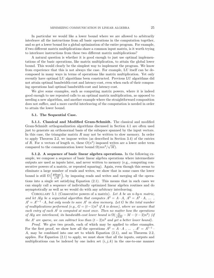
MINIMIZING COMMUNICATION IN LINEAR ALGEBRA 25
In particular we would like a lower bound where we are allowed to arbitrarilyinterleave all the instructions from all basic operations in the computation together,and so get a lower bound for a global optimization of the entire program. For example,if two different matrix multiplications share a common input matrix, is it worth tryingto interleave instructions from these two different matrix multiplications?
A natural question is whether it is good enough to just use optimal implemen-tations of the basic operations, like matrix multiplication, to attain the global lowerbound. This would clearly be the simplest way to implement the program. We knowfrom experience that this is not always the case. For example, LU itself can be de-composed in many ways in terms of operations like matrix multiplication. Yet onlyrecently have optimal LU algorithms been constructed. Previous LU algorithms didnot attain optimal bandwidth-cost and latency-cost, even when each of their compos-ing operations had optimal bandwidth-cost and latency-cost.
We give some examples, such as computing matrix powers, where it is indeedgood enough to use repeated calls to an optimal matrix multiplication, as opposed toneeding a new algorithm, and another example where the straightforward compositiondoes not suffice, and a more careful interleaving of the computation is needed in orderto attain the lower bound.
5.1. The Sequential Case.
5.1.1. Classical and Modified Gram-Schmidt. The classical and modifiedGram-Schmidt orthogonalization algorithms discussed in Section 4.1 are often usedjust to generate an orthonormal basis of the subspace spanned by the input vectors.In this case, the triangular matrix R may not be written to slow memory. In orderto apply Theorem 2.2, we impose writes (as described in Section 3.4) of the entriesof R. For n vectors of length m, these O(n2) imposed writes are a lower order termcompared to the communication lower bound Ω(mn2/
√M).
5.1.2. A sequence of basic linear algebra operations. In the following ex-ample, we compose a sequence of basic linear algebra operations where intermediateoutputs are used as inputs later, and never written to memory (e.g., computing con-secutive powers of a matrix, or repeated squaring). Again, even though this seems toeliminate a large number of reads and writes, we show that in some cases the lowerbound is still Ω
(#flops√
M
), by imposing reads and writes and merging all the opera-
tions into a single set satisfying Equation (2.1). This means that in such cases wecan simply call a sequence of individually optimized linear algebra routines and doasymptotically as well as we would do with any arbitrary interleaving.
Corollary 5.1 (Consecutive powers of a matrix). Let A be an n-by-n matrix,and let Alg be a sequential algorithm that computes A2 = A · A, A3 = A2 · A, ... ,At = At−1 ·A, but only needs to save At in slow memory. Let G be the total numberof multiplications performed (e.g., G = (t−1)n3 if A is dense), where we assume thateach entry of each Ai is computed at most once. Then no matter how the operationsof Alg are interleaved, its bandwidth-cost lower bound is Ω( G√
8M−M − (t− 2)n2) (if
the Ai are sparse, we can subtract less than (t− 2)n2 and get a better lower bound).Proof. We give two proofs, each of which may be applied to other examples.
For the first proof, we show how all the operations A2 = A · A , ... , At = At−1 ·A, may be combined into one set to which Equation (2.1), and so Theorem 2.2,applies. For Equation (2.1) to apply, we must show that all the inputs, outputs andmultiplications can be indexed by one index set (i, j, k) in the one-to-one manner
26 BALLARD, DEMMEL, HOLTZ, AND SCHWARTZ
described in section 2; this is most easily seen by writing all the operations asA2
A3
...At
=
AA2
...At−1
·ARecall that Equation (2.1) permits inputs and output to overlap, and “a(i, k)” and“b(k, j)” inputs to overlap, but the “a(i, k)” inputs alone must be indexed one-to-one,and similarly the “b(k, j)” inputs alone must be indexed one-to-one; this is the caseabove.
Next, we impose writes of all the intermediate results A2, ..., At−1, yielding a newalgorithm Alg′. This means that there are no R2/D2 arguments, so Theorem 2.2applies to Alg′. Thus the bandwidth-cost lower bound of Alg′ is G√
8M−M , and the
bandwidth-cost lower bound of Alg is lower by the number of imposed writes, at most(t− 2)n2 (less if the matrices are sparse).
Now we present a second proof, which uses the Loomis-Whitney-based analysisof a segment more directly. We let #Ai be the number of entries of Ai in fastmemory during a segment of Alg′. From the definition of a segment, we can bound∑t
i=1 #Ai ≤ 4M . Applying Loomis-Whitney to each multiplication Ai+1 = Ai·A thatone might do (some of) during a segment, we can bound the number of multiplicationsduring a segment by F =
∑t−1i=1
√#Ai+1 ·#Ai ·#A1. We can now bound F subject
to the constraint∑t
i=1 #Ai ≤ 4M , yielding
F =t−1∑i=1
√#Ai+1 ·#Ai ·#A1
=√
#A1 ·t−1∑i=1
√#Ai+1 ·#Ai
≤√
#A1 ·
√√√√t−1∑i=1
#Ai+1 ·
√√√√t−1∑i=1
#Ai ... by the Cauchy − Schwarz inequality
≤√
4M ·√
4M ·√
4M = 8√M3
This yields the ultimate bandwidth-cost lower bound of G/(8√M)−M .
Both proof techniques also apply to repeated squaring: Ai+1 = A2i for i = 1, ..., t−
1, the first proof via the identityA2
A4
. . .A2t
=
A
A2
. . .A2t−1
·A
A2
. . .A2t−1
and the second proof by bounding the number of multiplications during a segment bymaximizing F =
∑t−1i=1
√#Ai ·#Ai ·#Ai+1 subject to
∑ti=1 #Ai ≤ 4M (here #Ai
denotes the number of entries of A2i−1available during a segment).
5.1.3. Interleaved vs. Phased Sequences of Operations. In some cases,one can combine and interleave basic linear algebra operations, (e.g., a sequence of
MINIMIZING COMMUNICATION IN LINEAR ALGEBRA 27
matrix multiplications) so that the resulting algorithm no longer agrees with Equa-tion (2.1), although the algorithms for performing each of the basic linear algebraoperations separately do agree with Equation (2.1). This may lead to an algorithmwhose minimum communication is not proportional to #flops, but asymptoticallybetter.
Before giving an example, we first observe that a “phased” algorithm, consistingof a sequence of calls to individually optimized basic linear algebra operations (likematrix multiplication), where each such basic linear algebra operation (phase) mustcomplete before the next can begin, can offer no such asymptotic improvements.Indeed, if we perform Alg1, ... ,Algt in phases, where Algi has bandwidth-cost lowerbound Bi, then the sequence has bandwidth-cost lower bound B =
∑ti=1Bi − 2(t −
1)M . If each Bi is proportional to the operation count of Algi, then B is proportionalto the total operation count. (The modest improvement 2(t−1)M arises since we canpossibly avoid a little communication by Algi+1 using the results left in fast memoryby Algi.)
Let us now look at an example, where the interleaved algorithm can do asymptot-ically less communication than the phased algorithm: Consider computing the densematrix multiplications C(k) = A ·B(k) for k = 1, 2, ..., t where B(k)
i,j = k√Bi,j .
The idea is that having both Ai,k and Bk,j in fast memory lets us do up to tevaluations of gijk. Moreover, the union of all these tn3 operations does not matchEquation (2.1), since the inputs Bk,j cannot be indexed in a one-to-one fashion.However, we can still give a non-trivial lower bound as follows, analyzing the algorithmsegment by segment. Let us begin with the lower bound, then show an algorithmattaining this lower bound.
No operands in a segment are R2/D2. By the same argument as in Section 2, amaximum of 4M arguments of A, B and any C(i)’s are available during a segment.We want to bound the number of gijk’s that we can do during such a segment. Let#A,#B and #C(i) denote the number of each type of argument available during thesegment. Then by Loomis-Whitney (applied t times) the maximum number of gijk’sis bounded by F =
∑ti=1
√#A ·#B ·#C(i). We want to maximize F subject to the
constraint #A+#B+∑t
i=1 #C(i) ≤ 4M . Applying Cauchy-Schwarz as before yields
F =√
#A ·√
#B ·t∑
i=1
√#C(i) ≤
√#A ·
√#B ·
√√√√ t∑i=1
#C(i) ·√t
≤√
4M ·√
4M ·√
4M ·√t = 8
√tM3
The number of segments is thus at least⌊
tn3
8M3/2t1/2
⌋and the number of memory
operations at least t1/2n3
8M1/2 −M . This is smaller than the “phased” lower bound for tmatrix multiplications in sequence, tn3
8√
M− tM , by an asymptotic factor of Θ(
√t).
We next show that this bound is indeed attainable, using a different blockedmatrix multiplication algorithm whose block sizes b1 and b2 depend on M and t (seeAlgorithm 1). The bandwidth-cost count for this algorithm is as follows. In theinnermost loop we read/write t blocks of C(1), ...., C(t), of M/3t words each. So wehave 2M/3 reads/writes for the innermost loop. Before this loop we read two blocks (ofA and B) of M/3 words each. This adds up to O(M) read/writes. This is performedn3
b21b2times. So the total bandwidth-cost count is O
(M ·
(n3
b21b2
))= O
(√tn3√
M
).
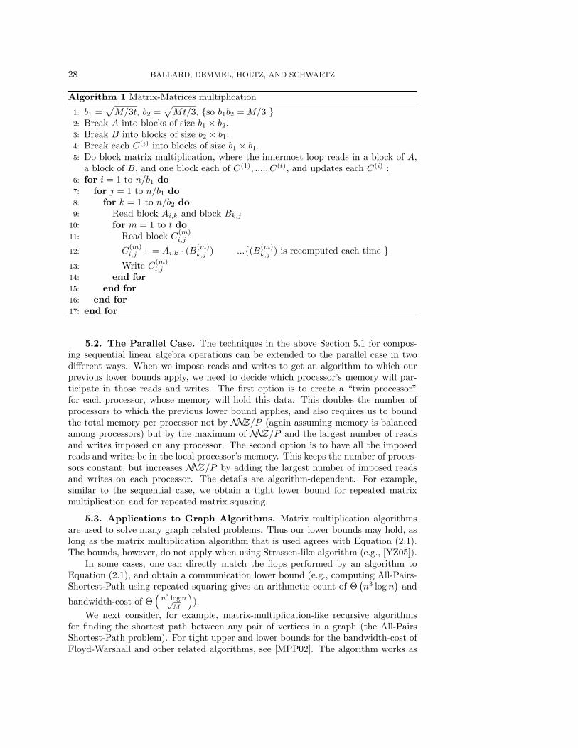
28 BALLARD, DEMMEL, HOLTZ, AND SCHWARTZ
Algorithm 1 Matrix-Matrices multiplication
1: b1 =√M/3t, b2 =
√Mt/3, so b1b2 = M/3
2: Break A into blocks of size b1 × b2.3: Break B into blocks of size b2 × b1.4: Break each C(i) into blocks of size b1 × b1.5: Do block matrix multiplication, where the innermost loop reads in a block of A,
a block of B, and one block each of C(1), ...., C(t), and updates each C(i) :6: for i = 1 to n/b1 do7: for j = 1 to n/b1 do8: for k = 1 to n/b2 do9: Read block Ai,k and block Bk,j
10: for m = 1 to t do11: Read block C(m)
i,j
12: C(m)i,j + = Ai,k · (B(m)
k,j ) ...(B(m)k,j ) is recomputed each time
13: Write C(m)i,j
14: end for15: end for16: end for17: end for
5.2. The Parallel Case. The techniques in the above Section 5.1 for compos-ing sequential linear algebra operations can be extended to the parallel case in twodifferent ways. When we impose reads and writes to get an algorithm to which ourprevious lower bounds apply, we need to decide which processor’s memory will par-ticipate in those reads and writes. The first option is to create a “twin processor”for each processor, whose memory will hold this data. This doubles the number ofprocessors to which the previous lower bound applies, and also requires us to boundthe total memory per processor not by NNZ/P (again assuming memory is balancedamong processors) but by the maximum of NNZ/P and the largest number of readsand writes imposed on any processor. The second option is to have all the imposedreads and writes be in the local processor’s memory. This keeps the number of proces-sors constant, but increases NNZ/P by adding the largest number of imposed readsand writes on each processor. The details are algorithm-dependent. For example,similar to the sequential case, we obtain a tight lower bound for repeated matrixmultiplication and for repeated matrix squaring.
5.3. Applications to Graph Algorithms. Matrix multiplication algorithmsare used to solve many graph related problems. Thus our lower bounds may hold, aslong as the matrix multiplication algorithm that is used agrees with Equation (2.1).The bounds, however, do not apply when using Strassen-like algorithm (e.g., [YZ05]).
In some cases, one can directly match the flops performed by an algorithm toEquation (2.1), and obtain a communication lower bound (e.g., computing All-Pairs-Shortest-Path using repeated squaring gives an arithmetic count of Θ
(n3 log n
)and
bandwidth-cost of Θ(
n3 log n√M
)).
We next consider, for example, matrix-multiplication-like recursive algorithmsfor finding the shortest path between any pair of vertices in a graph (the All-PairsShortest-Path problem). For tight upper and lower bounds for the bandwidth-cost ofFloyd-Warshall and other related algorithms, see [MPP02]. The algorithm works as

MINIMIZING COMMUNICATION IN LINEAR ALGEBRA 29
follows [CLRS01]. Let l(m)ij be the minimum weight of any path from vertex i to vertex
j that contains at most m edges, where the weight of the edge (i, j) is wij = l(1)ij . Then
l(m)ij = min1≤k≤n
(l(m−1)ik + wkj
), and the recursive naive algorithm for the All-Pairs
Shortest-Path problems performs exactly these Θ(n4) computations. If all values l(m)ij
are written to slow memory, then, by Theorem 2.2, the bandwidth-cost lower boundis Ω
(n4√
M
). Although this may not be the case —some of the intermediate values
may never reach the slow memory— there are fewer than n3 intermediate l(m)ij values.
Thus, by imposing reads and writes, the bandwidth-cost lower bound is Ω(
n4√
M
)(note
that here, similar to the repeated matrix multiplication arguments of Corollary 5.1,after imposing writes, no two gijk operations use the same two inputs, so Equation2.1 applies). Similarly, the Θ(n3 log n) recursive algorithm for APSP has O(n2 log n)intermediate values, therefore, by Theorem 2.2 and imposing reads and writes, thebandwidth-cost lower bound is Ω
(n3 log n√
M
).
Note that these lower bounds are attainable. As noted before (see e.g., [CLRS01])any matrix powering algorithm can be converted into a APSP algorithm, by us-ing ‘+’ instead of ‘∗’ and ‘min’ instead of summation. Starting with any of thecommunication-avoiding optimal matrix-multiplication algorithms (e.g., [FLPR99])guarantees a bandwidth-cost upper bound of O
(n4√
M
)and O
(n3 log n√
M
)respectively.
Using recursive-block data structure further guarantees optimal latency-cost for bothalgorithms.
The above repeated-matrix-squaring-like algorithm may, in some cases, performbetter than the communication-avoiding implementation of Floyd-Warshall algorithm[MPP02]. Consider the problem of finding the neighbors within distance t of everyvertex.
One can use the above repeated-matrix-squaring-like algorithm for log t phases,obtaining a running time of Θ(n3 log t) and communication cost Θ
(n3 log t√
M
)for dense
graphs. For sparse input graphs this may be further reduced. For example, when Gis a union of cycles and paths, the running time and communication bandwidth-costare O(n22t) and O
(n22t√
M
)(as the degree of a vertex of the ith phase is at most 22i
).
If, however, we use the Floyd-Warshall algorithm for this purpose, we have torun it all the way through, regardless of the input graph, resulting in running timeof Θ(n3) and communication cost of Θ
(n3√
M
)(assuming the above communication-
avoiding implementation). Thus, for t = o(log n) the repeated-matrix-squaring-likealgorithm performs better for constant-degree inputs, both from flops count and fromcommunication bandwidth-cost perspectives.
6. Attaining the lower bounds, and open problems. A major problem isto find algorithms that attain the lower bounds described in this paper, for bandwidthand latency costs, for the various linear algebra problems, for dense and sparse ma-trices, and for sequential and parallel machines. And since real computers generallyhave many levels of memory hierarchy, and possibly levels of parallelism as well (coreson a chip, chips in a node, nodes in a rack, racks in a room...) we would ideally like tominimize communication between all of them simultaneously (i.e., between L1 and L2cache, between L2 cache and main memory, between memories of different processors,and so on). It is easy to see that our lower bounds can be applied hierarchically to
30 BALLARD, DEMMEL, HOLTZ, AND SCHWARTZ
this situation, for example, by treating L1 and L2 cache as “fast memory” and L3cache and DRAM as “slow memory”, to bound below memory traffic between L3 andL2 cache.
Tables 6.1 and 6.2 summarize the current state-of-the-art (to the best of ourknowledge) for the communication cost of algorithms for dense matrices. To sum-marize, in the dense sequential case (Table 6.1), for most important problems, thelower bounds are attained for 2 levels of memory hierarchy (excluding Gram–Schmidtand modified Gram–Schmidt algorithms), but fewer are attained so far for multiplelevels, at least without constant factor increases in the amount of arithmetic. Inthe dense parallel case (Table 6.2), for most important problems, the lower boundsare also attained (again, excluding Gram–Schmidt and modified Gram–Schmidt al-gorithms), assuming minimal memory O(n2/P ) per processor, and modulo polylogPterms. Again, some of these algorithms do a constant factor times as much arithmeticas their conventional counterparts.
However, only a few of these communication-optimal algorithms appear in stan-dard libraries like LAPACK [ABB+92] and ScaLAPACK [BCC+97]; the complexityof ScaLAPACK implementations in Table 6.2 is taken from [BCC+97, Table 5.8].(Other libraries may well attain similar bounds [GGHvdG01, vdG].) Several of thepapers cited below report large speedups compared to these standard libraries.
When there is enough memory per processor for c > 1 copies of the data (M =cn2/p instead of M = n2/p), the lower bound on the number of words decreases by afactor of c1/2 and the lower bound on the number of messages decreases by a factorc3/2. So far only a few algorithms are known that achieve these smaller lower bounds,for dense matrix multiplication and (just for the number of words) LU decomposition[SD11, MT99, DNS81, ABG+95]. (We note that c cannot be arbitrarily large; theproof breaks down when the lower bound on the number of messages reaches 1, i.e.,c reaches p1/3.)
We note that in practice, a collection of words must be stored in contiguous lo-cations in order to be transferred as a single message at maximum bandwidth; this isa consequence of common hardware design limitations. On a parallel computer, theprocessor can in principle repack locally stored noncontiguous data into a separatecontiguous region before sending it to another processor. But on a sequential com-puter, the data structure must have the property that desired data (a submatrix, say)is already stored contiguously. But if a matrix is stored row-wise or column-wise, thenmost submatrices (those not consisting of complete rows or columns) will not havethis property. This means that in order to achieve the lower bound on the number ofmessages, sequential algorithms must not store matrices row-wise or column-wise, butblock-wise. And in order to to minimize the number of messages when there is morethan one level of memory hierarchy, these blocks must themselves be stored block-wise, leading to data structures known by various names in the literature, such asrecursive block layout or storage using space-filling curves or Morton-ordered quadtreematrices [EGJK04]. The algorithms referred to in Table 6.1 as minimizing the numberof messages assume such data-structures are used.
One may imagine that sequential algorithms that minimize communication forany number of levels of memory hierarchy might be very complex, possibly dependingnot just on the number of levels, but their sizes. It is worth distinguishing a class ofalgorithms, called cache-oblivious [FLPR99], that can sometimes minimize communi-cation between all levels (at least asymptotically) independent of the number of levelsand their sizes. These algorithms are recursive, for example multiplying two n-by-
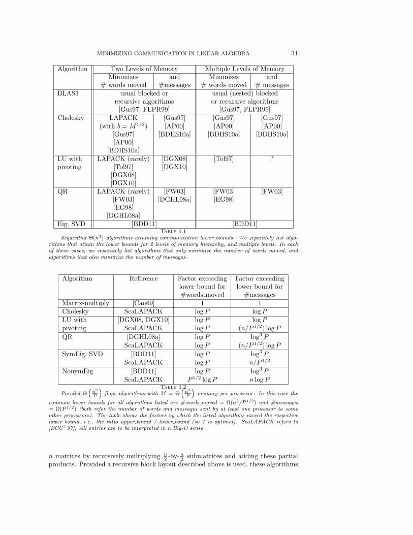
MINIMIZING COMMUNICATION IN LINEAR ALGEBRA 31
Algorithm Two Levels of Memory Multiple Levels of MemoryMinimizes and Minimizes and
# words moved #messages # words moved # messagesBLAS3 usual blocked or usual (nested) blocked
recursive algorithms or recursive algorithms[Gus97, FLPR99] [Gus97, FLPR99]
Cholesky LAPACK [Gus97] [Gus97] [Gus97](with b = M1/2) [AP00] [AP00] [AP00]
[Gus97] [BDHS10a] [BDHS10a] [BDHS10a][AP00]
[BDHS10a]LU with LAPACK (rarely) [DGX08] [Tol97] ?pivoting [Tol97] [DGX10]
[DGX08][DGX10]
QR LAPACK (rarely) [FW03] [FW03] [FW03][FW03] [DGHL08a] [EG98][EG98]
[DGHL08a]Eig, SVD [BDD11] [BDD11]
Table 6.1Sequential Θ(n3) algorithms attaining communication lower bounds. We separately list algo-
rithms that attain the lower bounds for 2 levels of memory hierarchy, and multiple levels. In eachof these cases, we separately list algorithms that only minimize the number of words moved, andalgorithms that also minimize the number of messages.
Algorithm Reference Factor exceeding Factor exceedinglower bound for lower bound for#words moved #messages
Matrix-multiply [Can69] 1 1Cholesky ScaLAPACK logP logPLU with [DGX08, DGX10] logP logPpivoting ScaLAPACK logP (n/P 1/2) logPQR [DGHL08a] logP log3 P
ScaLAPACK logP (n/P 1/2) logPSymEig, SVD [BDD11] logP log3 P
ScaLAPACK logP n/P 1/2
NonymEig [BDD11] logP log3 PScaLAPACK P 1/2 logP n logP
Table 6.2Parallel Θ
“n3
P
”flops algorithms with M = Θ
“n2
P
”memory per processor: In this case the
common lower bounds for all algorithms listed are #words moved = Ω(n2/P 1/2) and #messages= Ω(P 1/2) (both refer the number of words and messages sent by at least one processor to someother processors). The table shows the factors by which the listed algorithms exceed the respectivelower bound, i.e., the ratio upper bound / lower bound (so 1 is optimal). ScaLAPACK refers to[BCC+97]. All entries are to be interpreted in a Big-O sense.
n matrices by recursively multiplying n2 -by-n
2 submatrices and adding these partialproducts. Provided a recursive block layout described above is used, these algorithms

32 BALLARD, DEMMEL, HOLTZ, AND SCHWARTZ
may also minimize the number of messages independent of the number of levels ofmemory hierarchy. All the algorithms cited in Table 6.1 that work for arbitrary levelsof memory hierarchy are cache-oblivious. (In practice one does not recur down to 1-by-1 submatrices because of the high overhead. Also, some cache-oblivious algorithmsrequire a constant factor more arithmetic operations than non-oblivious alternatives[FW03]. So “pure” cache-obliviousness is not a panacea.)
We now discuss these tables in more detail. There is a very large body of work onmany of these algorithms, and we do not pretend to have a complete list of citations.Instead we refer just to papers where these algorithms first appeared (to the best of ourknowledge), with or without analysis of their communication costs (often without),or to survey papers.
Best understood are dense matrix-multiplication, other BLAS routines, andCholesky, which have algorithms that attain (perhaps modulo polylogP factors) bothbandwidth and latency lower bounds on parallel machines, and on sequential ma-chines with multiple levels of memory hierarchy. The optimal sequential Choleskyalgorithm cited in Table 6.1 was presented in [Gus97, AP00], but first analyzed laterin [BDHS10a]. The algorithm in [AP00, BDHS10a] is cache-oblivious, but whetheror not the recursive algorithm in [Gus97] minimizes communication for many levelsof memory hierarchy depends on the implementation of the underlying BLAS librarythat it uses. The complexity of ScaLAPACK’s parallel Cholesky cited in Table 6.2assumes that the largest possible block size is chosen (NB ≈ n/
√P in line “PxPOSV”
in [BCC+97, Table 5.8]).More recently, optimal dense LU and QR algorithms have been proposed that
attain both bandwidth and latency lower bounds in parallel or sequentially (withjust 2 levels of memory hierarchy). LAPACK is labeled “rarely” because only forsome matrix dimensions n and fast memory sizes M is it possible to choose a blocksize b to attain the lower bound. Interestingly, conventional partial pivoting mustapparently be replaced by a different (but still stable) pivoting scheme in order tominimize latency costs in LU [DGX08, DGX10]; we can retain partial pivoting if weonly want to minimize bandwidth [Tol97]. Similarly, we must apparently change thestandard representation of the Q matrix in QR in order to minimize both latencyand bandwidth costs [DGHL08a]; we can retain the usual representation if we onlywant to minimize bandwidth costs in the sequential case [EG98]. Both [EG98] and[FW03] are cache oblivious, but only [FW03] also minimizes latency costs; howeverit triples the arithmetic operation count to do so. See the above references for largespeedups reported over algorithms that do not try to minimize communication. Theideas behind communication-optimal dense QR first appear in [GPS88], and include[BLKD07, GG05, EG98]; see [DGHL08a] for a more complete list of references.
ScaLAPACK’s parallel symmetric eigensolver and SVD routine also minimizebandwidth cost (modulo a logP factor), but not the latency cost, sending O(n/P 1/2)times as many messages. ScaLAPACK’s nonsymmetric eigensolver communicatesmuch more, indeed just the Hessenberg QR iteration has n-times higher latency cost.LAPACK’s symmetric and nonsymmetric eigensolvers and SVD minimize neitherbandwidth nor latency costs, moving O(n3) words. Recently proposed randomizedalgorithms in [BDD11, DDH07] for the symmetric and nonsymmetric eigenproblems,generalized nonsymmetric eigenproblems and SVD do attain the desired communica-tion cost (modulo polylogP factors) but at the cost of doing a possibly large constantfactor more arithmetic. (This is in contrast to the new dense LU and QR algorithms,which do at most O(n2) more arithmetic operations than the O(n3) operations done

MINIMIZING COMMUNICATION IN LINEAR ALGEBRA 33
by their conventional counterparts.) In [BDD11] it is also pointed out that appropriatevariants of the “successive band reduction” approach in [BLS00a, BLS00b] can alsominimize communication, at least in the sequential case for the symmetric eigenprob-lem and SVD, for a much smaller increase in the arithmetic operation count (nearlyno increase, if eigenvalues/singular values alone are desired).
The eigenvalue algorithms mentioned above use randomization to implement aURV decomposition that reveals the rank with high probability; here U and V areorthogonal and R is upper triangular, with the large singular values “in the upperleft corner” of R, and the small singular values “in the lower right corner.” In fact wecan perform an implicit randomized rank-revealing URV factorization on an arbitraryproduct
∏iA±1i without the need to multiply or invert any of the factors Ai, and so
retain numerical stability.Devising algorithms that attain the communication lower bounds while perform-
ing QR with column pivoting, LU with complete pivoting, or LDLT factorizationwith any pivoting remain work in progress. It also remains an open problem to designparallel algorithms (besides matrix multiplication and LU decomposition) that cantake advantage of extra memory (a multiple of the minimal n2/p per processor) tofurther reduce communication. Finally, finding optimal algorithms for heterogenouscomputers (eg CPUs and GPUs), where each processor has a different fast memorysize, bandwidth, latency and floating point speed, remains open.
It is possible to extend our lower bound results to many Strassen-like algorithms[BDHS10b] for matrix multiplication, which are attained by the natural recursivesequential implementations, and are attainable in parallel as well. But the lower boundproof is significantly different than the one used in this paper. By using recursivealgorithms in [DDH07], it is possible to compute LU, QR and other factorizationswhile doing asymptotially as little arithmetic and commucation (at least sequentially)as Strassen-like matrix multiplication. But it remain an open problem to extend thelower bounds to any implementation of “Strassen-like LU”, “Strassen-like QR”, etc.
For the Cholesky factorization of sparse matrices, whose sparsity structure sat-isfy certain graph-theoretic conditions (having “good separators”), the lower boundscan also be attained [DDGP10]. For sparse matrix algorithms more generally, theproblems are open.
We note that for sufficiently rectangular dense matrices (e.g., matrix-vector mul-tiplication) or for sufficiently sparse matrices (e.g., multiplying diagonal matrices),our lower bound may be lower than the trivial lower bound (#inputs + #outputs)and so not be attainable. In this case the natural question is whether the maximumof the two lower bounds is attainable (as it is for dense matrix multiplication).
Acknowledgments.The authors thank Cleve Ashcraft, Robert Luce, Nicholas Knight, Edgar Solomonik,
and Sivan Toledo for a number of helpful comments, questions and discussions, as wellas the anonymous reviewers for their valuable comments.

34 BALLARD, DEMMEL, HOLTZ, AND SCHWARTZ
REFERENCES
[ABB+92] E. Anderson, Z. Bai, C. Bischof, J. Demmel, J. Dongarra, J. Du Croz, A. Green-baum, S. Hammarling, A. McKenney, S. Ostrouchov, and D. Sorensen. LA-PACK’s user’s guide. Society for Industrial and Applied Mathematics, Philadel-phia, PA, USA, 1992. Also available from http://www.netlib.org/lapack/.
[ABG+95] R. C. Agarwal, S. M. Balle, F. G. Gustavson, M. Joshi, and P. Palkar. A three-dimensional approach to parallel matrix multiplication. IBM J. Res. Dev.,39:575–582, September 1995.
[AGW01] B. S. Andersen, F. Gustavson, and J. Wasniewski. A recursive formulation ofCholesky factorization of a matrix in packed storage format. ACM Transactionson Mathematical Software, 27(2):214–244, jun 2001.
[AP00] N. Ahmed and K. Pingali. Automatic generation of block-recursive codes. In Euro-Par ’00: Proceedings from the 6th International Euro-Par Conference on Par-allel Processing, pages 368–378, London, UK, 2000. Springer-Verlag.
[Ash91] C. Ashcraft. A taxonomy of distributed dense LU factorization methods. BoeingComputer Services Technical Report ECA-TR-161, March 1991.
[Ash93] C. Ashcraft. The fan-both family of column-based distributed Cholesky factorizationalgorithms. In John R. Gilbert Alan George and Joseph W. H. Liu, editors,Graph Theory and Sparse Matrix Computation, volume 56 of IMA Volumes inMathematics and its Applications, Springer-Verlag, pages 159–190, 1993.
[AV88] A. Aggarwal and J. S. Vitter. The input/output complexity of sorting and relatedproblems. Commun. ACM, 31(9):1116–1127, 1988.
[BBF+07] M. A. Bender, G. S. Brodal, R. Fagerberg, R. Jacob, and E. Vicari. Optimalsparse matrix dense vector multiplication in the I/O-model. In SPAA ’07:Proceedings of the nineteenth annual ACM symposium on parallel algorithmsand architectures, pages 61–70, New York, NY, USA, 2007. ACM.
[BBM02a] K. Braman, R. Byers, and R. Mathias. The Multi-Shift QR Algorithm, Part I:Maintaining Well Focused Shifts and Level 3 Performance. SIAM J. MatrixAnal. App., 23(4):929–947, 2002.
[BBM02b] K. Braman, R. Byers, and R. Mathias. The Multi-Shift QR Algorithm, Part II:Aggressive Early Deflation. SIAM J. Matrix Anal. App., 23(4):948–973, 2002.
[BCC+97] L. S. Blackford, J. Choi, A. Cleary, E. DAzevedo, J. Demmel, I. Dhillon, J. Don-garra, S. Hammarling, G. Henry, A. Petitet, K. Stanley, D. Walker, and R. C.Whaley. ScaLAPACK Users’ Guide. SIAM, Philadelphia, PA, USA, May 1997.Also available from http://www.netlib.org/scalapack/.
[BDD+01] L. S. Blackford, J. Demmel, J. Dongarra, I. Duff, S. Hammarling, G. Henry, M. Her-oux, L. Kaufman, A. Lumsdaine, A. Petitet, R. Pozo, K. Remington, R. C.Whaley, Z. Maany, F. Krough, G. Corliss, C. Hu, B. Keafott, W. Walster, andJ. Wolff v. Gudenberg. Basic Linear Algebra Subprograms Techical (BLAST)Forum Standard. Intern. J. High Performance Comput., 15(3-4), 2001.
[BDD+02] L. S. Blackford, J. Demmel, J. Dongarra, I. Duff, S. Hammarling, G. Henry, M. Her-oux, L. Kaufman, A. Lumsdaine, A. Petitet, R. Pozo, K. Remington, and R. C.Whaley. An updated set of Basic Linear Algebra Subroutines (BLAS). ACMTrans. Math. Soft., 28(2), June 2002.
[BDD11] G. Ballard, J. Demmel, and I. Dumitriu. Communication-optimal parallel andsequential eigenvalue and singular value algorithms. EECS Technical ReportEECS-2011-14, UC Berkeley, February 2011.
[BDHS10a] G. Ballard, J. Demmel, O. Holtz, and O. Schwartz. Communication-optimal paralleland sequential Cholesky decomposition. SIAM J. Sci. Comput., 32:3495–3523,2010.
[BDHS10b] G. Ballard, J. Demmel, O. Holtz, and O. Schwartz. Graph Expansion and Commu-nication Costs of Algorithms, 2010. Submitted.
[BK77] J. Bunch and L. Kaufman. Some stable methods for calculating inertia and solv-ing symmetric linear systems. Mathematics of Computation, 31(137):163–179,January 1977.
[BLKD07] A. Buttari, J. Langou, J. Kurzak, and J. J. Dongarra. A class of parallel tiled linearalgebra algorithms for multicore architectures. Technical Report 191, LAPACKWorking Note, September 2007.
[BLS00a] C. H. Bischof, B. Lang, and X. Sun. Algorithm 807: The SBR Toolbox—softwarefor successive band reduction. ACM Transactions on Mathematical Software,26(4):602–616, December 2000.

MINIMIZING COMMUNICATION IN LINEAR ALGEBRA 35
[BLS00b] C. H. Bischof, B. Lang, and X. Sun. A framework for symmetric band reduction.ACM Transactions on Mathematical Software, 26(4):581–601, December 2000.
[BVL87] C. Bischof and C. Van Loan. The WY representation for products of Householdermatrices. SIAM J. Sci. Stat. Comp., 8(1), 1987.
[BZ88] Y. D. Burago and V. A. Zalgaller. Geometric Inequalities, volume 285 ofGrundlehren der Mathematische Wissenschaften. Springer, Berlin, 1988.
[Can69] L. Cannon. A cellular computer to implement the Kalman filter algorithm. PhDthesis, Montana State University, Bozeman, MN, 1969.
[CLRS01] Thomas H. Cormen, Charles E. Leiserson, Ronald L. Rivest, and Clifford Stein.Introduction to Algorithms. The MIT Press, 2nd edition, 2001.
[CR06] R. A. Chowdhury and V. Ramachandran. Cache-oblivious dynamic programming.In SODA ’06: Proceedings of the seventeenth annual ACM-SIAM symposiumon discrete algorithms, pages 591–600, New York, NY, USA, 2006. ACM.
[DDGP10] P.-Y. David, J. Demmel, L. Grigori, and S. Peyronnet. Brief announcement: Lowerbounds on communication for sparse Cholesky factorization of a model prob-lem. In 22nd ACM Symposium on Parallelism in Algorithms and Architectures(SPAA), 2010.
[DDH07] J. Demmel, I. Dumitriu, and O. Holtz. Fast linear algebra is stable. NumerischeMathematik, 108(1):59–91, 2007.
[Dem96] J. Demmel. CS 267 Course Notes: Applications of Parallel Pro-cessing. Computer Science Division, University of California, 1996.http://www.cs.berkeley.edu/∼demmel/cs267.
[Dem97] J. Demmel. Applied Numerical Linear Algebra. SIAM, 1997.[DGHL08a] J. Demmel, L. Grigori, M. Hoemmen, and J. Langou. Communication-optimal par-
allel and sequential QR and LU factorizations. UC Berkeley Technical ReportEECS-2008-89, Aug 1, 2008; Submitted to SIAM. J. Sci. Comp., 2008.
[DGHL08b] J. Demmel, L. Grigori, M. Hoemmen, and J. Langou. Implementing communication-optimal parallel and sequential QR and LU factorizations. Submitted to SIAM.J. Sci. Comp., 2008.
[DGX08] J. Demmel, L. Grigori, and H. Xiang. Communication-avoiding Gaussian elimina-tion. Supercomputing 08, 2008.
[DGX10] J. Demmel, L. Grigori, and H. Xiang. CALU: A communication optimal LU factor-ization algorithm. EECS Technical Report EECS-2010-29, UC Berkeley, March2010. Submitted to SIAM J. Matrix Anal. Appl.
[DNS81] Eliezer Dekel, David Nassimi, and Sartaj Sahni. Parallel matrix and graph algo-rithms. SIAM Journal on Computing, 10(4):657–675, 1981.
[EG98] E. Elmroth and F. Gustavson. New serial and parallel recursive QR factorizationalgorithms for SMP systems. In B. Kagstrom et al., editor, Applied ParallelComputing. Large Scale Scientific and Industrial Problems., volume 1541 ofLecture Notes in Computer Science, pages 120–128. Springer, 1998.
[EGJK04] E. Elmroth, F. Gustavson, I. Jonsson, and B. Kagstrom. Recursive blocked algo-rithms and hybrid data structures for dense matrix library software. SIAMReview, 46(1):3–45, March 2004.
[FLPR99] M. Frigo, C. E. Leiserson, H. Prokop, and S. Ramachandran. Cache-oblivious al-gorithms. In FOCS ’99: Proceedings of the 40th Annual Symposium on Foun-dations of Computer Science, page 285, Washington, DC, USA, 1999. IEEEComputer Society.
[FW03] J. D. Frens and D. S. Wise. QR factorization with Morton-ordered quadtree matricesfor memory re-use and parallelism. SIGPLAN Not., 38(10):144–154, 2003.
[Geo73] A. George. Nested dissection of a regular finite element mesh. SIAM J. Numer.Anal., 10:345–363, 1973.
[GG05] B. C. Gunter and R. A. Van De Geijn. Parallel out-of-core computation and updat-ing of the QR factorization. ACM Trans. Math. Softw., 31(1):60–78, 2005.
[GGHvdG01] J. A. Gunnels, F. G. Gustavson, G. M. Henry, and R. A. van de Geijn. FLAME:Formal Linear Algebra Methods Environment. ACM Transactions on Mathe-matical Software, 27(4):422–455, December 2001.
[GPS88] G. H. Golub, R. J. Plemmons, and A. Sameh. Parallel block schemes for large-scaleleast-squares computations. In High-speed computing: scientific applicationsand algorithm design, pages 171–179, Champaign, IL, USA, 1988. University ofIllinois Press.
[GT87] J. R. Gilbert and R. E. Tarjan. The analysis of a nested dissection algorithm.Numerische Mathematik, pages 377–404, 1987.

36 BALLARD, DEMMEL, HOLTZ, AND SCHWARTZ
[Gus97] F. G. Gustavson. Recursion leads to automatic variable blocking for dense linear-algebra algorithms. IBM J. Res. Dev., 41(6):737–756, 1997.
[GVL96] G. Golub and C. Van Loan. Matrix Computations. Johns Hopkins University Press,Baltimore, MD, 3rd edition, 1996.
[HK81] J. W. Hong and H. T. Kung. I/O complexity: The red-blue pebble game. InSTOC ’81: Proceedings of the thirteenth annual ACM symposium on theory ofcomputing, pages 326–333, New York, NY, USA, 1981. ACM.
[HMR73] A. J. Hoffman, M. S. Martin, and D. J. Rose. Complexity bounds for regular finitedifference and finite element grids. SIAM J. Numer. Anal., 10:364–369, 1973.
[IT02] D. Irony and S. Toledo. Trading replication for communication in paralleldistributed-memory dense solvers. Parallel Processing Letters, 12(1):79–94,2002.
[ITT04] D. Irony, S. Toledo, and A. Tiskin. Communication lower bounds for distributed-memory matrix multiplication. J. Parallel Distrib. Comput., 64(9):1017–1026,2004.
[LW49] L. H. Loomis and H. Whitney. An inequality related to the isoperimetric inequality.Bulletin of the AMS, 55:961–962, 1949.
[MPP02] J. P. Michael, M. Penner, and V. K. Prasanna. Optimizing graph algorithms for im-proved cache performance. In In Proc. Intl Parallel and Distributed ProcessingSymp. (IPDPS 2002), Fort Lauderdale, FL, pages 769–782, 2002.
[MT99] W. F. McColl and A. Tiskin. Memory-efficient matrix multiplication in the BSPmodel. Algorithmica, 24:287–297, 1999.
[Pug92] C. Puglisi. Modification of the Householder method based on compact WY repre-sentation. SIAM J. Sci. Stat. Comput., 13(3):723–726, 1992.
[Saa86] Y. Saad. Communication complexity of the Gaussian elimination algorithm onmultiprocessors. Linear Algebra Appl., 77:315–340, 1986.
[Saa96] Y. Saad. Iterative Methods for Sparse Linear Systems. PWS Publishing Co., Boston,1996.
[Sav95] J. E. Savage. Extending the Hong-Kung model to memory hierarchies. In COCOON,pages 270–281, 1995.
[SD11] E. Solomonik and J. Demmel. Communication-optimal parallel 2.5D matrix mul-tiplication and LU factorization algorithms. EECS Technical Report EECS-2011-10, UC Berkeley, February 2011.
[SVL89] R. Schreiber and C. Van Loan. A storage efficient WY representation for productsof Householder transformations. SIAM J. Sci. Stat. Comput., 10:53–57, 1989.
[Tol97] S. Toledo. Locality of reference in LU decomposition with partial pivoting. SIAMJ. Matrix Anal. Appl., 18(4):1065–1081, 1997.
[vdG] R. van de Geijn. PLAPACK: Parallel Linear Algebra Package.www.cs.utexas.edu/users/plapack.
[VDY05] R. Vuduc, J. Demmel, and K. Yelick. OSKI: A library of automatically tuned sparsematrix kernels. In Proc. of SciDAC 2005, J. of Physics: Conference Series.Institute of Physics Publishing, June 2005.
[YZ05] R. Yuster and U. Zwick. Fast sparse matrix multiplication. ACM Trans. Algorithms,1(1):2–13, 2005.
Appendix A. Motivation for 1× 1 T matrices.In the proof of Theorem 4.10, we make an assumption that all T matrices in-
volved in blocked Householder updates of the form A = (I−UTUT )A are 1×1. Thisassumption seems like a significant restriction, since blocked Householder transfor-mations are widely used in practice. We do not believe this assumption is necessaryfor the communication lower bound to be valid, but the reason for the assumptionis that we discovered an artificial example, where by using an O(n4) algorithm withO(n4) additional storage (to form and use a T matrix of dimension O(n2)) on a cer-tain matrix, we could arrange to have one segment in which O(M2) multiplicationswere performed, thereby creating an obstacle to our proof technique, which dependson bounding the number of multiplications per segment by O(M3/2). This (imprac-tical!) variant of QR is not a counterexample to our theorem overall, just our prooftechnique. We present the example here.
Consider an n× 2n matrix A = [A1, A2] where A1 is square and dense and A2 is

MINIMIZING COMMUNICATION IN LINEAR ALGEBRA 37
square and nonzero only in its last row. Then A has the following sparsity structure:
0 5 10 15 20
0
2
4
6
8
10
nz = 110
A
Suppose we perform QR on A using Givens rotations, where we work column bycolumn, rotating the bottom row into the one above it, that row into the one aboveit, and so on to the diagonal entry. There will be n(n−1)
2 Givens rotations, and if weindex them as described in Section 4, then the U matrix will have n(n−1)
2 columnswith the following sparsity structure:
0 5 10 15 20 25 30 35 40 45
0
5
10
nz = 90
U
Suppose the computation is organized so that the triangularization of A1 is com-pleted before any updates are done to A2. By letting T be as large as possible andfollowing equation (4.2) the update of A2 can be written as
A2 = A2 −∑
k
U(:, k) · Z(k, :)
where Z = TUTA2. Here, T is n(n−1)2 × n(n−1)
2 and at least 25% nonzero, and thesparsity structure of Z and its factors are given below.
0 20 40
0
10
20
30
40
nz = 825
T
0 5 10
0
10
20
30
40
nz = 90
UT
0 5 10
0
5
10
nz = 10
A2
0 5 10
0
10
20
30
40
nz = 450
Z
* * =
Thus, the computation A2 = A2 − UZ has the following structure:

38 BALLARD, DEMMEL, HOLTZ, AND SCHWARTZ
0 5 10
0
5
10
nz = 10
A2
0 20 40
05
10
nz = 90
U
0 5 10
0
10
20
30
40
nz = 450
Z
*-
The full computation will completely fill in A2, but suppose in one segment weonly update the last two rows of A2 by choosing the subset S of the columns of U andcorresponding rows of Z which effect only the last two rows. Note that |S| = n − 1.In this case, the subcomputation is of the form
A2(n− 1 : n, j) = A2(n− 1 : n, j)−∑k∈S
U(n− 1 : n, k) · Z(k, j)
which has the following sparsity structure:
0 5 10
0
5
10
nz = 10
A2
0 5 10
0
5
10
nz = 18
U(:,S)
0 5 10
0
5
10
nz = 90
Z(S,:)
*-
Further, all the entries of Z can be R2/D2. Each Z(k, j) is the dot product of arow of (TUT ) with a column of A2. Due to the sparsity structure of A2, this is justone scalar multiplication. If we pre-compute (TUT ) and store it in slow memory, thenin one segment we could do the following:
1: read A2(n, :), (TUT )(S, n), and U(n− 1 : n, S) from slow memory2: for j = 1 to n do3: for k ∈ S do4: Z(k, j) = (TUT )(k, n) ·A2(n, j)5: A2(n− 1 : n, j) = A2(n− 1 : n, j)− U(n− 1 : n, k) · Z(k, j)6: discard Z(k, j)7: end for8: end for
In this way, if n = M/5, then the last two rows of A2, the entries of the lastcolumn of (TUT ) in rows k ∈ S, and the last two rows of U in columns k ∈ S can allfit into fast memory simultaneously, and the O(M2) corresponding Z entries can becomputed, used to update A2, and discarded as shown above.
Thus, modeling the computation with the form A = A − U · Z and allowingunbounded T matrices, this example shows that it is possible to execute O(M2) flopswithin a single segment (allowing only O(M) memory operations). This motivatesour restriction that the T matrices are all 1 × 1. However, we do not believe this isa counterexample to the lower bound result because it involves the computation andstorage of O(n4) entries of T .
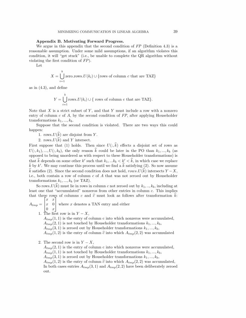
MINIMIZING COMMUNICATION IN LINEAR ALGEBRA 39
Appendix B. Motivating Forward Progress.We argue in this appendix that the second condition of FP (Definition 4.3) is a
reasonable assumption. Under some mild assumptions, if an algorithm violates thiscondition, it will “get stuck” (i.e., be unable to complete the QR algorithm withoutviolating the first condition of FP).
Let
X =b⋃
i=1
zero rows U(ki) ∪ rows of column c that are TAZ
as in (4.3), and define
Y =b⋃
i=1
rows U(ki) ∪ rows of column c that are TAZ.
Note that X is a strict subset of Y , and that Y must include a row with a nonzeroentry of column c of A, by the second condition of FP, after applying Householdertransformations k1, ..., kb.
Suppose that the second condition is violated. There are two ways this couldhappen:
1. rows U(k) are disjoint from Y .2. rows U(k) and Y intersect.
First suppose that (1) holds. Then since U(:, k) effects a disjoint set of rows asU(:, k1), ..., U(:, kb), the only reason k could be later in the PO than k1, ..., kb (asopposed to being unordered as with respect to these Householder transformations) isthat k depends on some other k′ such that k1, ...kb < k′ < k, in which case we replacek by k′. We may continue this process until we find a k satisfying (2). So now assumek satisfies (2). Since the second condition does not hold, rows U(k) intersects Y −X,i.e., both contain a row of column c of A that was not zeroed out by Householdertransformations k1, ..., kb (or TAZ).
So rows U(k) must lie in rows in column c not zeroed out by k1, .., kb, including atleast one that “accumulated” nonzeros from other entries in column c. This impliesthat three rows of columns c and c must look as follows after transformation k:
Atmp =
x xx 00 x
where x denotes a TAN entry and either
1. The first row is in Y −X,Atmp(1, 1) is the entry of column c into which nonzeros were accumulated,Atmp(2, 1) is not touched by Householder transformations k1, ..., kb,Atmp(3, 1) is zeroed out by Householder transformations k1, ..., kb,Atmp(1, 2) is the entry of column c into which Atmp(2, 2) was accumulated
2. The second row is in Y −X,Atmp(2, 1) is the entry of column c into which nonzeros were accumulated,Atmp(1, 1) is not touched by Householder transformations k1, ..., kb,Atmp(3, 1) is zeroed out by Householder transformations k1, ..., kb,Atmp(1, 2) is the entry of column c into which Atmp(2, 2) was accumulated,In both cases entries Atmp(3, 1) and Atmp(2, 2) have been deliberately zeroedout.
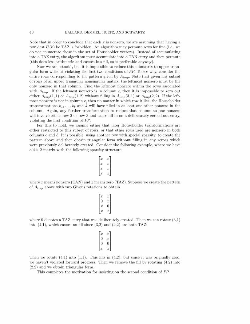
40 BALLARD, DEMMEL, HOLTZ, AND SCHWARTZ
Note that in order to conclude that each x is nonzero, we are assuming that having arow dest U(k) be TAZ is forbidden. An algorithm may permute rows for free (i.e., wedo not enumerate those in the set of Householder vectors). Instead of accumulatinginto a TAZ entry, the algorithm must accumulate into a TAN entry and then permute(this does less arithmetic and causes less fill, so is preferable anyway).
Now we are “stuck”, i.e., it is impossible to reduce this submatrix to upper trian-gular form without violating the first two conditions of FP. To see why, consider theentire rows corresponding to the pattern given by Atmp. Note that given any subsetof rows of an upper triangular nonsingular matrix, the leftmost nonzero must be theonly nonzero in that column. Find the leftmost nonzero within the rows associatedwith Atmp. If the leftmost nonzero is in column c, then it is impossible to zero outeither Atmp(1, 1) or Atmp(1, 2) without filling in Atmp(3, 1) or Atmp(2, 2). If the left-most nonzero is not in column c, then no matter in which row it lies, the Householdertransformations k1, . . . , kb and k will have filled in at least one other nonzero in thecolumn. Again, any further transformation to reduce that column to one nonzerowill involve either row 2 or row 3 and cause fill-in on a deliberately-zeroed-out entry,violating the first condition of FP.
For this to hold, we assume either that later Householder transformations areeither restricted to this subset of rows, or that other rows used are nonzero in bothcolumns c and c. It is possible, using another row with special sparsity, to create thepattern above and then obtain triangular form without filling in any zeroes whichwere previously deliberately created. Consider the following example, where we havea 4× 2 matrix with the following sparsity structure:
x xx xx xx z
where xmeans nonzero (TAN) and z means zero (TAZ). Suppose we create the patternof Atmp above with two Givens rotations to obtain
x x0 xx 0x z
where 0 denotes a TAZ entry that was deliberately created. Then we can rotate (3,1)into (4,1), which causes no fill since (3,2) and (4,2) are both TAZ:
x x0 x0 0x z
Then we rotate (4,1) into (1,1). This fills in (4,2), but since it was originally zero,we haven’t violated forward progress. Then we remove the fill by rotating (4,2) into(2,2) and we obtain triangular form.
This completes the motivation for insisting on the second condition of FP.