numerical linear algebra a solution manual · numerical linear algebra a solution manual georg...

Numerical Linear Algebra

A Solution Manual

Georg Muntingh and Christian Schulz

Contents

Chapter 0. A Short Review of Linear Algebra 1Exercise 0.25: The inverse of a general 2× 2 matrix 1Exercise 0.26: The inverse of a 2× 2 matrix 1Exercise 0.27: Sherman-Morrison formula 1Exercise 0.29: Cramer’s rule; special case 1Exercise 0.30: Adjoint matrix; special case 1Exercise 0.31: Determinant equation for a plane 2Exercise 0.32: Signed area of a triangle 2Exercise 0.33: Vandermonde matrix 3Exercise 0.34: Cauchy determinant 3Exercise 0.35: Inverse of the Hilbert matrix 5

Chapter 1. Diagonally dominant tridiagonal matrices; three examples 7Exercise 1.12: The shifted power basis is a basis 7Exercise 1.25: LU factorization of 2nd derivative matrix 7Exercise 1.26: Inverse of 2nd derivative matrix 8Exercise 1.27: Central difference approximation of 2nd derivative 8Exercise 1.28: Two point boundary value problem 9Exercise 1.29: Two point boundary value problem; computation 9Exercise 1.30: Approximate force 10Exercise 1.38: Matrix element as a quadratic form 10Exercise 1.39: Outer product expansion of a matrix 10Exercise 1.40: The product ATA 10Exercise 1.41: Outer product expansion 10Exercise 1.42: System with many right hand sides; compact form 11Exercise 1.43: Block multiplication example 11Exercise 1.44: Another block multiplication example 11

Chapter 2. Gaussian eliminations and LU Factorizations 12Exercise 2.8: Column oriented backsolve 12Exercise 2.11: Computing the inverse of a triangular matrix 12Exercise 2.13: Finite sums of integers 14Exercise 2.14: Multiplying triangular matrices 15Exercise 2.23: Row interchange 16Exercise 2.24: LU and determinant 16Exercise 2.25: Diagonal elements in U 16Exercise 2.31: Making a block LU into an LU 17Exercise 2.36: Using PLU of A to solve ATx = b 18Exercise 2.37: Using PLU to compute the determinant 18Exercise 2.38: Using PLU to compute the inverse 18

i

Chapter 3. LDL* Factorization and Positive definite Matrices 19Exercise 3.20: Positive definite characterizations 19

Chapter 4. Orthonormal and Unitary Transformations 20Exercise 4.4: The ATA inner product 20Exercise 4.5: Angle between vectors in complex case 20Exercise 4.18: What does Algorithm housegen do when x = e1? 20Exercise 4.19: Examples of Householder transformations 21Exercise 4.20: 2× 2 Householder transformation 21Exercise 4.28: QR decomposition 22Exercise 4.29: Householder triangulation 22Exercise 4.32: QR using Gram-Schmidt, II 23Exercise 4.34: Plane rotation 23Exercise 4.35: Solving upper Hessenberg system using rotations 24

Chapter 5. Eigenpairs and Similarity Transformations 25Exercise 5.9: Idempotent matrix 25Exercise 5.10: Nilpotent matrix 25Exercise 5.11: Eigenvalues of a unitary matrix 25Exercise 5.12: Nonsingular approximation of a singular matrix 25Exercise 5.13: Companion matrix 26Exercise 5.17: Find eigenpair example 26Exercise 5.22: Jordan example 26Exercise 5.24: Properties of the Jordan form 27Exercise 5.25: Powers of a Jordan block 27Exercise 5.27: Big Jordan example 28Exercise 5.30: Schur decomposition example 28Exercise 5.34: Skew-Hermitian matrix 28Exercise 5.35: Eigenvalues of a skew-Hermitian matrix 28Exercise 5.49: Eigenvalue perturbation for Hermitian matrices 29Exercise 5.51: Hoffman-Wielandt 29Exercise 5.54: Biorthogonal expansion 29Exercise 5.57: Generalized Rayleigh quotient 29

Chapter 6. The Singular Value Decomposition 30Exercise 6.7: SVD examples 30Exercise 6.8: More SVD examples 31Exercise 6.16: Counting dimensions of fundamental subspaces 31Exercise 6.17: Rank and nullity relations 32Exercise 6.18: Orthonormal bases example 32Exercise 6.19: Some spanning sets 33Exercise 6.20: Singular values and eigenpair of composite matrix 33Exercise 6.26: Rank example 33Exercise 6.27: Another rank example 34

Chapter 7. Norms and Perturbation theory for linear systems 36Exercise 7.7: Consistency of sum norm? 36Exercise 7.8: Consistency of max norm? 36Exercise 7.9: Consistency of modified max norm? 36Exercise 7.11: The sum norm is subordinate to? 37

ii

Exercise 7.12: The max norm is subordinate to? 38Exercise 7.19: Spectral norm 38Exercise 7.20: Spectral norm of the inverse 38Exercise 7.21: p-norm example 39Exercise 7.24: Unitary invariance of the spectral norm 39Exercise 7.25: ‖AU‖2 rectangular A 39Exercise 7.26: p-norm of diagonal matrix 39Exercise 7.27: Spectral norm of a column vector 40Exercise 7.28: Norm of absolute value matrix 40Exercise 7.35: Sharpness of perturbation bounds 41Exercise 7.36: Condition number of 2nd derivative matrix 41Exercise 7.47: When is a complex norm an inner product norm? 43Exercise 7.48: p-norm for p = 1 and p =∞ 44Exercise 7.49: The p-norm unit sphere 45Exercise 7.50: Sharpness of p-norm inequality 45Exercise 7.51: p-norm inequalities for arbitrary p 45

Chapter 8. Least Squares 47Exercise 8.10: Fitting a circle to points 47Exercise 8.17: The generalized inverse 48Exercise 8.18: Uniqueness of generalized inverse 48Exercise 8.19: Verify that a matrix is a generalized inverse 48Exercise 8.20: Linearly independent columns and generalized inverse 49Exercise 8.21: The generalized inverse of a vector 49Exercise 8.22: The generalized inverse of an outer product 49Exercise 8.23: The generalized inverse of a diagonal matrix 50Exercise 8.24: Properties of the generalized inverse 50Exercise 8.25: The generalized inverse of a product 50Exercise 8.26: The generalized inverse of the conjugate transpose 51Exercise 8.27: Linearly independent columns 51Exercise 8.28: Analysis of the general linear system 51Exercise 8.29: Fredholm’s Alternative 52Exercise 8.32: Condition number 52Exercise 8.35: Problem using normal equations 53

Chapter 9. The Kronecker Product 54Exercise 9.2: 2× 2 Poisson matrix 54Exercise 9.5: Properties of Kronecker products 54Exercise 9.9: 2nd derivative matrix is positive definite 55Exercise 9.10: 1D test matrix is positive definite? 55Exercise 9.11: Eigenvalues for 2D test matrix of order 4 56Exercise 9.12: Nine point scheme for Poisson problem 56Exercise 9.13: Matrix equation for nine point scheme 57Exercise 9.14: Biharmonic equation 58

Chapter 10. Fast Direct Solution of a Large Linear System 60Exercise 10.5: Fourier matrix 60Exercise 10.6: Sine transform as Fourier transform 60Exercise 10.7: Explicit solution of the discrete Poisson equation 61

iii

Exercise 10.8: Improved version of Algorithm 10.1 61Exercise 10.9: Fast solution of 9 point scheme 62Exercise 10.10: Algorithm for fast solution of 9 point scheme 63Exercise 10.11: Fast solution of biharmonic equation 63Exercise 10.12: Algorithm for fast solution of biharmonic equation 64Exercise 10.13: Check algorithm for fast solution of biharmonic equation 64

Chapter 11. The Classical Iterative Methods 66Exercise 11.12: Richardson and Jacobi 66Exercise 11.13: Convergence of the R-method when eigenvalues have positivereal part 66Exercise 11.16: Example: GS converges, J diverges 66Exercise 11.17: Divergence example for J and GS 67Exercise 11.18: Strictly diagonally dominance; The J method 67Exercise 11.19: Strictly diagonally dominance; The GS method 68Exercise 11.23: Convergence example for fix point iteration 68Exercise 11.24: Estimate in Lemma 11.22 can be exact 69Exercise 11.25: Slow spectral radius convergence 69Exercise 11.31: A special norm 71Exercise 11.33: When is A + E nonsingular? 71

Chapter 12. The Conjugate Gradient Method 72Exercise 12.1: A-norm 72Exercise 12.2: Paraboloid 72Exercise 12.5: Steepest descent iteration 72Exercise 12.8: Conjugate gradient iteration, II 73Exercise 12.9: Conjugate gradient iteration, III 74Exercise 12.10: The cg step length is optimal 74Exercise 12.11: Starting value in cg 74Exercise 12.17: Program code for testing steepest descent 75Exercise 12.18: Using cg to solve normal equations 77Exercise 12.23: Krylov space and cg iterations 78Exercise 12.26: Another explicit formula for the Chebyshev polynomial 79Exercise 12.28: Maximum of a convex function 79

Chapter 13. Numerical Eigenvalue Problems 80Exercise 13.5: Nonsingularity using Gerschgorin 80Exercise 13.6: Gerschgorin, strictly diagonally dominant matrix 80Exercise 13.8: Continuity of eigenvalues 80Exercise 13.12: ∞-norm of a diagonal matrix 81Exercise 13.15: Number of arithmetic operations 81Exercise 13.17: Number of arithmetic operations 81Exercise 13.18: Tridiagonalize a symmetric matrix 82Exercise 13.22: Counting eigenvalues 82Exercise 13.23: Overflow in LDLT factorization 83Exercise 13.24: Simultaneous diagonalization 83Exercise 13.25: Program code for one eigenvalue 84Exercise 13.26: Determinant of upper Hessenberg matrix (TODO) 85

Chapter 14. The QR Algorithm 86

iv

Exercise 14.4: Orthogonal vectors 86

v

CHAPTER 0

A Short Review of Linear Algebra

Exercise 0.25: The inverse of a general 2× 2 matrix

A straightforward computation yields

1

ad− bc

[d −b−c a

] [a bc d

]=

1

ad− bc

[ad− bc 0

0 ad− bc

]=

[1 00 1

],

showing that the two matrices are inverse to each other.

Exercise 0.26: The inverse of a 2× 2 matrix

By Exercise 0.25, and using that cos2 θ + sin2 θ = 1, the inverse is given by[cos θ sin θ− sin θ cos θ

].

Exercise 0.27: Sherman-Morrison formula

A direct computation yields

(A + BCT)(A−1 −A−1B(I + CTA−1B)−1CTA−1

)= I−B(I + CTA−1B)−1CTA−1 + BCTA−1 −BCTA−1B(I + CTA−1B)−1CTA−1

= I + BCTA−1 −B(I + CTA−1B)(I + CTA−1B)−1CTA−1

= I + BCTA−1 −BCTA−1

= I,

showing that the two matrices are inverse to each other.

Exercise 0.29: Cramer’s rule; special case

Cramer’s rule yields

x1 =

∣∣∣∣3 26 1

∣∣∣∣ / ∣∣∣∣1 22 1

∣∣∣∣ = 3, x2 =

∣∣∣∣1 32 6

∣∣∣∣ / ∣∣∣∣1 22 1

∣∣∣∣ = 0.

Exercise 0.30: Adjoint matrix; special case

We are given the matrix

A =

2 −6 33 −2 −66 3 2

.1

Computing the cofactors of A gives

adjTA =

(−1)1+1

∣∣∣∣−2 −63 2

∣∣∣∣ (−1)1+2

∣∣∣∣3 −66 2

∣∣∣∣ (−1)1+3

∣∣∣∣3 −26 3

∣∣∣∣(−1)2+1

∣∣∣∣−6 33 2

∣∣∣∣ (−1)2+2

∣∣∣∣2 36 2

∣∣∣∣ (−1)2+3

∣∣∣∣2 −66 3

∣∣∣∣(−1)3+1

∣∣∣∣−6 3−2 −6

∣∣∣∣ (−1)3+2

∣∣∣∣2 33 −6

∣∣∣∣ (−1)3+3

∣∣∣∣2 −63 −2

∣∣∣∣

=

14 21 42−42 −14 2121 −42 14

T

.

One checks directly that adjAA = det(A)I, with det(A) = 343.

Exercise 0.31: Determinant equation for a plane

Let ax+ by+ cz+ d = 0 be an equation for a plane through the points (xi, yi, zi), withi = 1, 2, 3. There is precisely one such plane if and only if the points are not colinear.Then axi + byi + czi + d = 0 for i = 1, 2, 3, so that

x y z 1x1 y1 z1 1x2 y2 z2 1x3 y3 z3 1

abcd

=

0000

.Since the coordinates a, b, c, d of the plane are not all zero, the above matrix is sin-gular, implying that its determinant is zero. Computing this determinant by cofactorexpansion of the first row gives the equation

+

∣∣∣∣∣∣y1 z1 1y2 z2 1y3 z3 1

∣∣∣∣∣∣x−∣∣∣∣∣∣x1 z1 1x2 z2 1x3 z3 1

∣∣∣∣∣∣ y +

∣∣∣∣∣∣x1 y1 1x2 y2 1x3 y3 1

∣∣∣∣∣∣ z −∣∣∣∣∣∣x1 y1 z1x2 y2 z2x3 y3 z3

∣∣∣∣∣∣ = 0

of the plane.

Exercise 0.32: Signed area of a triangle

Let T denote the triangle with vertices P1, P2, P3. Since the area of a triangle isinvariant under translation, we can assume P1 = A = (0, 0), P2 = (x2, y2), P3 = (x3, y3),B = (x3, 0), and C = (x2, 0). As is clear from Figure 1, the area A(T ) can be expressedas

A(T ) = A(ABP3) + A(P3BCP2)− A(ACP2)

=1

2x3y3 + (x2 − x3)y2 +

1

2(x2 − x3)(y3 − y2)−

1

2x2y2

=1

2

∣∣∣∣∣∣1 1 10 x2 x30 y2 y3

∣∣∣∣∣∣ ,which is what needed to be shown.

2

Exercise 0.33: Vandermonde matrix

For any n = 1, 2, . . ., let

Dn :=

∣∣∣∣∣∣∣∣∣∣

1 x1 x21 · · · xn−11

1 x2 x22 · · · xn−12

1 x3 x23 · · · xn−13...

......

. . ....

1 xn x2n · · · xn−1n

∣∣∣∣∣∣∣∣∣∣be the determinant of the Vandermonde matrix in the Exercise. Clearly the formula

(?) DN =∏

1≤j<i≤N

(xi − xj)

holds for N = 1 (in which case the product is empty and defined to be 1) and N = 2.Let us assume (?) holds for N = n−1 > 2. Since the determinant is an alternating

multilinear form, adding a scalar multiple of one column to another does not changethe value of the determinant. Subtracting xkn times column k from column k + 1 fork = n− 1, n− 2, . . . , 1, we find

Dn =

∣∣∣∣∣∣∣∣∣∣

1 x1 − xn x21 − x1xn · · · xn−11 − xn−21 xn1 x2 − xn x22 − x2xn · · · xn−12 − xn−22 xn1 x3 − xn x23 − x3xn · · · xn−13 − xn−23 xn...

......

. . ....

1 xn − xn x2n − xnxn · · · xn−1n − xn−2n xn

∣∣∣∣∣∣∣∣∣∣.

Next, by cofactor expansion along the last row and by the multilinearity in the rows,

Dn = (−1)n−1 · 1 ·

∣∣∣∣∣∣∣∣x1 − xn x21 − x1xn · · · xn−11 − xn−21 xnx2 − xn x22 − x2xn · · · xn−12 − xn−22 xn

......

. . ....

xn−1 − xn x2n−1 − xn−1xn · · · xn−1n−1 − xn−2n−1xn

∣∣∣∣∣∣∣∣= (−1)n−1(x1 − xn)(x2 − xn) · · · (xn−1 − xn)Dn−1

= (xn − x1)(xn − x2) · · · (xn − xn−1)∏

1≤j<i≤n−1

(xi − xj)

=∏

1≤j<i≤n

(xi − xj).

By induction, we conclude that (?) holds for any N = 1, 2, . . .

Exercise 0.34: Cauchy determinant

(a) Let [α1, . . . , αn]T, [β1, . . . , βn]T ∈ Rn and let

A = (ai,j)i,j =

(1

αi + βj

)i,j

=

1

α1+β11

α1+β2· · · 1

α1+βn1

α2+β11

α2+β2· · · 1

α2+βn...

.... . .

...1

αn+β11

αn+β2· · · 1

αn+βn

.3

Multiplying the ith row of A by∏n

k=1(αi + βk) for i = 1, 2, . . . , n gives a matrix

C = (ci,j)i,j, ci,j =n∏k=1k 6=j

(αi + βk).

The determinant of an n × n matrix is a homogeneous polynomial of degree n in theentries of the matrix. Since each entry of C is a polynomial of degree n − 1 in thevariables αi, βj, the determinant of C must be a homogeneous polynomial of degreen(n− 1) in αi, βj.

By the multilinearity of the determinant, det C =∏n

i,j=1(αi + βj) det A. Since Avanishes whenever αi = αj or βi = βj for i 6= j, the homogeneous polynomial det Ccontains factors (αi − αj) and (βi − βj) for 1 ≤ i < j ≤ n. As there are precisely2 ·(n2

)= (n− 1)n such factors, necessarily

(?) det C = k∏

1≤i<j≤n

(αi − αj)∏

1≤i<j≤n

(βi − βj)

for some constant k. To determine k, we can evaluate det C at a particular value, forinstance any αi, βji,j satisfying α1 +β1 = · · · = αn +βn = 0. In that case C becomesa diagonal matrix with determinant

det C =n∏i=1

n∏k=1k 6=i

(αi+βk) =n∏i=1

n∏k=1k 6=i

(αi−αk) =∏

1≤i<k≤n

(αi−αk)∏

1≤i<k≤n

(αk−αi).

Comparing with (?) shows that k = 1. We conclude that

(??) det A =

∏1≤i<j≤n

(αi − αj)∏

1≤i<j≤n

(βi − βj)

n∏i,j=1

(αi + βj)

.

(b) Deleting row l and column k from A, results in the matrix Al,k associated tothe vectors [α1, . . . , αl−1, αl+1, . . . , αn] and [β1, . . . , βk−1, βk+1, . . . , βn]. By the adjoint

4

formula for the inverse A−1 = (bk,l) and by (??),

bk,l := (−1)k+ldet Al,k

det A

= (−1)k+l

n∏i,j=1

(αi + βj)∏

1≤i<j≤ni,j 6=l

(αi − αj)∏

1≤i<j≤ni,j 6=k

(βi − βj)

n∏i,j=1i 6=lj 6=k

(αi + βj)∏

1≤i<j≤n

(αi − αj)∏

1≤i<j≤n

(βi − βj)

= (αl + βk)

n∏s=1s 6=l

(αs + βk)

n∏s=1s 6=l

(αs − αl)

n∏s=1s 6=k

(βs + αl)

n∏s=1s 6=k

(βs − βk)

= (αl + βk)n∏s=1s 6=l

αs + βkαs − αl

n∏s=1s 6=k

βs + αlβs − βk

,

which is what needed to be shown.

Exercise 0.35: Inverse of the Hilbert matrix

If we write

α = [α1, . . . , αn] = [1, 2, . . . , n], β = [β1, . . . , βn] = [0, 1, . . . , n− 1],

then the Hilbert matrix matrix is of the form Hn = (hi,j) =(1/(αi+βj)

). By Exercise

0.34.(b), its inverse Tn = (tni,j) := H−1n is given by

tni,j = (i+ j − 1)n∏s=1s 6=j

s+ i− 1

s− j

n∏s=1s 6=i

s+ j − 1

s− i, 1 ≤ i, j ≤ n.

We wish to show that

(?) tni,j =f(i)f(j)

i+ j − 1, 1 ≤ i, j ≤ n,

where f : N −→ Q is the sequence defined by

f(1) = −n, f(i+ 1) =

(i2 − n2

i2

)f(i), for i = 1, 2, . . . .

5

Clearly (?) holds when i = j = 1. Suppose that (?) holds for some (i, j). Then

tni+1,j = (i+ j)n∏s=1s 6=j

s+ 1 + i− 1

s− j

n∏s=1s 6=i+1

s+ j − 1

s− 1− i

= (i+ j)1

(i+ j)2

n+1∏s=2

(s+ i− 1)

n∏s=1s 6=j

(s− j)

n∏s=1

(s+ j − 1)

n−1∏s=0s 6=i

(s− i)

=(i+ j − 1)2(n+ i)(n− i)

(i+ j)i(−i)

n∏s=1s 6=j

(s+ i− 1)

n∏s=1s 6=j

(s− j)

n∏s=1s 6=i

(s+ j − 1)

n∏s=1s 6=i

(s− i)

=1

i+ j

i2 − n2

i2(i+ j − 1)

n∏s=1s 6=j

s+ i− 1

s− j(i+ j − 1)

n∏s=1s 6=i

s+ j − 1

s− i

=1

i+ j

i2 − n2

i2f(i)f(j)

=f(i+ 1)f(j)

(i+ 1) + j − 1,

so that (?) holds for (i+ 1, j). Carrying out a similar calculation for (i, j+ 1), or usingthe symmetry of Tn, we conclude by induction that (?) holds for any i, j.

6

CHAPTER 1

Diagonally dominant tridiagonal matrices; three examples

Exercise 1.12: The shifted power basis is a basis

We know that the set of polynomials of degree n is a vector space of dimension n+ 1:They are spanned by xknk=0, and these are linearly independent (if a linear combina-tion of these is zero, then it has in particular n+ 1 zeros (since every x is a zero), andit follows from the fundamental theorem of algebra that the linear combination mustbe zero). Since the shifted power basis also has n + 1 vectors which are polynomials,all we need to show is that they are linearly independent. Suppose then that

n∑j=0

aj(x− xi)j = 0.

In particular we can then pick n + 1 distinct values zk for x so that this is zero. Butthen the polynomial

∑nj=0 ajx

j has the n+ 1 different zeros zk − xi. Since the xknk=0

are linearly independent, it follows that all aj = 0, so that the shifted power basis alsois a basis.

Exercise 1.25: LU factorization of 2nd derivative matrix

Let L = (lij)ij,U = (rij)ij and T be as in the exercise. Clearly L is unit lowertriangular and U is upper triangular. We compute the product LU by separating casesfor its entries. There are several ways to carry out and write down this computation,some more precise than others. For instance,

(LU)11 = 1 · 2 = 2;

(LU)ii = −i− 1

i· −1 + 1 · i+ 1

i= 2, for i = 2, . . . ,m;

(LU)i,i−1 = −i− 1

i· i

i− 1= −1, for i = 2, . . . ,m;

(LU)i−1,i = 1 · −1 = −1, for i = 2, . . . ,m;

(LU)ij = 0, for |i− j| ≥ 2.

It follows that T = LU is an LU factorization.One can also show this by induction using the trifactor-algorithm. Since T

and U have the same super-diagonal, we must have cm = −1 for all m. Assume nowthat LmUm = Tm, and that lm−1 = −(m − 1)/m and um = (m + 1)/m. From thetrifactor-algorithm,

lm = am/um = −1/((m+ 1)/m) = −m/(m+ 1)

um+1 = dm+1 − lmcm = 2−m/(m+ 1) = (m+ 2)/(m+ 1).

This shows that the trifactor-algorithm produces the desired terms in Lm+1 andUm+1 as well.

7

Another way to show this by induction is as follows. For m = 1, one has L1U1 =1 · 2 = T1. Now let m > 1 be arbitrary and assume that LmUm = Tm. With

a := [0, . . . , 0,− m

m+ 1]T, b := [0, . . . , 0,−1]T,

block multiplication yields

Lm+1Um+1 =

[Lm 0aT 1

] [Um b0 m+2

m+1

]=[Tm Lmb

aTUm aTb + m+2m+1

]=

[Tm bbT 2

]= Tm+1.

By induction, we can then conclude that Tm = LmUm for all m ≥ 1.

Exercise 1.26: Inverse of 2nd derivative matrix

Let S = (sij)ij be defined by

sij = sji =1

m+ 1j(m+ 1− i) =

(1− i

m+ 1

)j, for 1 ≤ j ≤ i ≤ m.

In order to show that S = T−1, we multiply S by T and show that the result is theidentity matrix. To simplify notation we define sij := 0 whenever i = 0, i = m + 1,j = 0, or j = m+ 1. With 1 ≤ j < i ≤ m, we find(

ST)i,j

=m∑k=1

si,kTk,j = −si,j−1 + 2si,j − si,j+1

=

(1− i

m+ 1

)(−j + 1 + 2j − j − 1) = 0,

(ST)j,i

=m∑k=1

sj,kTk,i = −sj,i−1 + 2sj,i − sj,i+1

= −(

1− i− 1

m+ 1

)j + 2

(1− i

m+ 1

)j −

(1− i+ 1

m+ 1

)j

= −j + 2j − j + j · i− 1− 2i+ i+ 1

m+ 1= 0,

(ST)i,i

=m∑k=1

si,kTk,i = −si,i−1 + 2si,i − si,i+1

= −(

1− i

m+ 1

)(i− 1) + 2

(1− i

m+ 1

)i−(

1− i+ 1

m+ 1

)i = 1

which means that ST = I. Moreover, since S,T, and I are symmetric, transposingthis equation yields TS = I. We conclude that S = T−1.

Exercise 1.27: Central difference approximation of 2nd derivative

If all hi equal to the same number h, then

λi = µi =2h

h+ h= 1, δi =

yi+1 − yih

, βi = 3(δi−1 + δi) = 3yi+1 − yi−1

h,


8

Exercise 1.28: Two point boundary value problem

(a) For j = 1, . . . ,m, we get when we gather terms that

h2f(xj) =

(−1− h

2r(xj)

)vj−1 + (2 + h2q(xj))vj +

(−1 +

h

2r(xj)

)vj+1

From this we get the desired formula for aj, cj, and dj, and the right hand sides bj for2 ≤ j ≤ m− 1.For j = 1, since v0 is known we have to move

(−1− h

2r(x0)

)v0 = a1g0 over to the right

hand side, so that we obtain b0 = h2f(x1)− a1g0.For j = m, since vm+1 is known we have to move

(−1 + h

2r(xm)

)vm+1 = cmg1 over

to the right hand side, so that we obtain bm = h2f(xm) − cmg1. This leads to thetridiagonal system Av = b in the exercise.

(b) One has When h|r(x)|/2 < 1 for all x ∈ [a, b], we see that a, j, cj ∈ (−2, 0). Itfollows that |aj|+ |cj| = 1 + h

2r(xm) + 1 + h

2r(xm) = 2. Since q(xj) ≥ 0, |dj| = dj ≥ 2,

so that A is weakly diagonally dominant. Since |cj| = 1 + h2r(xj) < 2, and |dj| > 2 it

follows in particular that |d1| > |c1|. Clearly also all aj > 0 since h|r(x)|/2 < 1, andsince also |dj| > 2, in particular dn 6= 0, so that all the conditions in the theorem arefulfilled.

(c) We can use the method trisolve to find the v1, . . . , vm. Note that the indexingof the aj should be shifted with one in this exercise, to be compatible with the notationused in tridiag(aj, dj, cj) (aj and dj have the same index when they are in thesame column of the matrix. In this exercise they have the same index when they arein the same row).

Exercise 1.29: Two point boundary value problem; computation

(a) and (c) The provided values for r, f, q give that aj = cj = −1, dj = 2 + h2. Theinitial conditions are g0 = 1, g1 = 0, so that b = (h2 + 1, h2, . . . , h2). The code canlook as follows

for m = [9 19 39 79, 159]h = 1/(m+1);x = h*(1:m)’;[l, u] = trifactor( -ones(1, m - 1), (2+h 2)*ones(1, m), -ones(1, m - 1));b = h 2*ones(m, 1); b(1) = b(1) + 1;v = trisolve(l, u, -ones(1, m - 1), b);err = max(abs( (1-sinh(x)/sinh(1)) - v))log(err)/log(h)

end

The code also solves (c); If the error is proportional to hp, then err = Chp for someC. But then p = (log(err) − logC)/ log h ≈ log(err)/ log h for small h, which is thequantity computed inside the for-loop. It seems that this converges to 3, so that onewould guess that the error is proportional to h3.

(b)

m = 9h = 1/(m+1);x = h*(1:m)’;

9

[l, u] = trifactor( -ones(1, m - 1), (2+h 2)*ones(1, m), -ones(1, m - 1));b = h 2*ones(m, 1); b(1) = b(1) + 1;v = trisolve(l, u, -ones(1, m - 1), b);plot(x, (1-sinh(x)/sinh(1)), x, v)legend(’Exact solution’, ’Estimated solution’)

Exercise 1.30: Approximate force

Since sinx has Taylor series x − x3/3! + x5/5! − . . ., We have that sin(πh/2) =πh/2 + O(h3). If we square both sides we obtain sin2(πh/2) = π2h2/4 + O(h4). Fromthis we obtain that 4 sin2(πh/2)R/(h2L2) = π2R/L2 +O(h2).

Exercise 1.38: Matrix element as a quadratic form

Write A = (aij)ij and ei = (δik)k, where

δik =

1 if i = k,0 otherwise,

is the Kronecker delta. Then, by the definition of the matrix product,

eTi Aej = eT

i (Aej) = eTi

(∑k

alkδjk

)l

= eTi (alj)l =

∑l

δilalj = aij.

Exercise 1.39: Outer product expansion of a matrix

Clearly eieTj is the matrix Ei,j with 1 at entry (i, j), and zero elsewhere. Clearly also

A =∑

i,j ai,jEi,j =∑

i,j ai,jeieTj .

Exercise 1.40: The product ATA

A matrix product is defined as long as the dimensions of the matrices are compatible.More precisely, for the matrix product AB to be defined, the number of columns in Amust equal the number of rows in B.

Let now A be an n×m matrix. Then AT is an m×n matrix, and as a consequencethe product B := ATA is well defined. Moreover, the (i, j)-th entry of B is given by

(B)ij =(ATA

)ij

=n∑k=1

akiakj = aT.ia.j = 〈a.i, a.j〉,

which is what was needed to be shown.

Exercise 1.41: Outer product expansion

Recall that the matrix product of A ∈ Cm,n and BT = C ∈ Cn,p is defined by

(AC)ij =n∑k=1

aikckj =n∑k=1

aikbjk.

10

For the outer product expansion of the columns of A and B, on the other hand, wefind

(a:kb

T:k

)ij

= aikbjk. It follows that(ABT

)ij

=n∑k=1

aikbjk =n∑k=1

(a:kb

T:k

)ij.

Exercise 1.42: System with many right hand sides; compact form

Let A,B, and X be as in the Exercise.(=⇒): Suppose AX = B. Multiplying this equation from the right by ej yields

Ax.j = b.j for j = 1, . . . , p.(⇐=): Suppose Ax.j = b.j for j = 1, . . . , p. Let I = Ip denote the identity matrix.

Then

AX = AXI = AX[e1, . . . , ep] = [AXe1, . . . ,AXep]

= [Ax.1, . . . ,Ax.p] = [b.1, . . . ,b.p] = B.

Exercise 1.43: Block multiplication example

The product AB of two matrices A and B is defined precisely when the number ofcolumns of A is equal to the number of rows of B. For both sides in the equationAB = A1B1 to make sense, both pairs (A,B) and (A1,B1) need to be compatible inthis way. Conversely, if the number of columns of A equals the number of rows of Band the number of columns of A1 equals the number of rows of B1, then there existsintegers m, p, n, and s with 1 ≤ s ≤ p such that

A ∈ Cm,p, B ∈ Cp,n, A1 ∈ Cm,s, A2 ∈ Cm,p−s, B1 ∈ Cs,n.

Then

(AB)ij =

p∑k=1

aikbkj =s∑

k=1

aikbkj +

p∑k=s+1

aik · 0 = (A1B1)ij.

Exercise 1.44: Another block multiplication example

Since the matrices have compatible dimensions, a direct computation gives

CAB =

[1 0T

0 C1

] [λ aT

0 A1

] [1 0T

0 B1

]=

[λ aT

0 C1A1

] [1 0T

0 B1

]=

[λ aTB1

0 C1A1B1

].

11

CHAPTER 2

Gaussian eliminations and LU Factorizations

Exercise 2.8: Column oriented backsolve

If A is upper triangular, suppose that we after n − k steps of the algorithm havereduced our system to one of the form

a1,1 a1,2 · · · a1,k0 a2,1 · · · a2,k...

.... . .

...0 0 · · · ak,k

x1x2...xk

=

b1b2...bk

Clearly then xk = bk/ak,k (this explains the first statement inside the for-loop). Elim-inating the xk-variable we obtain the system

a1,1 a1,2 · · · a1,k−10 a2,1 · · · a2,k−1...

.... . .

...0 0 · · · ak−1,k−1

x1x2...

xk−1

=

b1b2...

bk−1

− xk

a1,ka2,k

...ak−1,k

.This means that the right hand side b should be updated by subtractingA(1:(k-1),k)*x(k). If A is d-banded, A1,k = · · · = Ak−d−1,k = 0, so that this isthe same as subtracting A(lk:(k-1),k)*x(k) with lk being the maximum of 1and k− d. This explains the second part inside the for-loop. Finally we end up witha 1× 1-matrix, so to find x1 we only need to divide with a1,1.

Exercise 2.11: Computing the inverse of a triangular matrix

This exercise introduces an efficient method for computing the inverse B of a triangularmatrix A.

Let us solve the problem for an upper triangular matrix (the lower triangular caseis similar). By the rules of block multiplication,

[Ab1, . . . ,Abn] = A[b1, . . . ,bn] = AB = I = [e1, . . . , en].

The kth column in this matrix equation says that Abk = ek. Let bk = (b1k, . . . , bnk)T.

Since the last n−k components of ek are 0, back subsitution yields that bk+1,k = . . . =bn,k = 0, so that B is upper triangular (as stated also by Lemma 1.35). Splitting A into

blocks

[A11 A12

0 A22

]where A11 has size k× k (A11 and A22 are then upper triangular),

12

we get

[A11 A12

0 A22

]

b1k...bkk0...0

=

A11

b1k...bkk

0

=

[ek0

],

so that we need to solve

A11

b1k...bkk

=

a11 · · · a1,k

0. . .

...0 0 ak,k

b1k...bkk

= ek.(1)

This yields (2.10) for solving for the kth column of B (note that the Matlab notationI(1 : k, k) yields ek).

Let us consider the number of arithmetic operations needed to compute the inverse.In finding bk we need to solve a k × k triangular system. Solving for x1 we need tocompute k − 1 multiplications, k − 2 additions, and one division. This gives a totalnumber of 2k− 2 arithmetic operations. Solving for x2 needs 2k− 4 operations, and soon, all the way down to xk−1 which needs 2 operations. Solving for xk = 1/ak,k needsan additional division, so that we need to perform

1 +k−1∑r=1

2r = 1 + (k − 1)k

operations. Since we solve a triangular system for any 1 ≤ k ≤ n, we end up with atotal of

n∑k=1

(1 + (k − 1)k) = n+n∑k=1

(k − 1)k = n+1

3(n− 1)n(n+ 1) =

1

3n(n2 + 2).

arithmetic operations. Here we used the formulas we deduced in Exercise 2.13.Usually we are just interesting in the “leading term” for the number of opera-

tions (here n3/3). This can be obtained more simply by approximating the sumswith integrals as in the book: solving the k × k triangular system can be solved in

1 +∑k−1

r=1 2r ≈∫ k−1r=1

2r ≈ (k− 1)2 ≈ k2 operations, and adding together the number of

operations for all k we obtain∑n

k=1 k2 ≈

∫ nk=1

k2dk ≈ n3/3 operations.Performing this block multiplication for k = n, n − 1, . . . , 1, we see that the com-

putations after step k only use the first k − 1 leading principal submatrices of A. Itfollows that the column bk computed at step k can be stored in row (or column) kof A without altering the remaining computations. A Matlab implementation whichstores the inverse (in-place) in A can thus look as follows:

n = 8;A = rand(n);A = triu(A);U=A;for k=n:-1:1

U(k,k) = 1/U(k,k);for r=k-1:-1:1

13

U(r, k) = -U(r,r+1:k)*U(r+1:k,k)/U(r,r);end

endU*A

A Python implementation can look as follows:

from numpy import *

n = 8A = matrix(random.random((n,n)))A=triu(A)U=A.copy()for k in range(n-1,-1,-1):

U[k,k] = 1/U[k,k]for r in range(k-1,-1,-1):

U[r, k] = -U[r,(r+1):(k+1)]*U[(r+1):(k+1),k]/U[r,r]print U*A

In the code, r and k are row- and column indices, respecively. Inside the for-loop wecompute xr for the system in Equation (1). The contribution from xr+1, . . . , xk canbe written as a dot product, which here is computed as a matrix product (the minussign comes from that we isolate xr on the left hand side). Note that k goes from n anddownwards. If we did this the other way we would overwrite matrix entries needed forlater calculations.

Exercise 2.13: Finite sums of integers

There are many ways to prove these identities. The quickest is perhaps by induction.We choose instead an approach based on what is called a generating function. Thisapproach does not assume knowledge of the sum-expressions we want to derive, andthe approach also works in a wide range of other circumstances.

It is easily checked that the identities hold for m = 1, 2, 3. So let m ≥ 4 and define

Pm(x) := 1 + x+ · · ·+ xm =1− xm+1

1− x.

Then

P ′m(x) =1− (m+ 1)xm +mxm+1

(x− 1)2,

P ′′m(x) =−2 + (m2 +m)xm−1 + 2(1−m2)xm + (m2 −m)xm+1

(x− 1)3.

14

Applying l’Hopital’s rule twice, we find

1 + 2 + · · ·+m = P ′m(1)

= limx→1

1− (m+ 1)xm +mxm+1

(x− 1)2

= limx→1

−m(m+ 1)xm−1 +m(m+ 1)xm

2(x− 1)

=1

2m(m+ 1),

establishing (2.12). In addition it follows that

1 + 3 + · · ·+ 2m− 1 =m∑k=1

(2k − 1) = −m+ 2m∑k=1

k = −m+m(m+ 1) = m2,

which establishes (2.14). Next, applying l’Hopital’s rule three times, we find that

1 · 2 + 2 · 3 + · · ·+ (m− 1) ·m = P ′′m(1)

is equal to

limx→1

−2 + (m2 +m)xm−1 + 2(1−m2)xm + (m2 −m)xm+1

(x− 1)3

= limx→1

(m− 1)(m2 +m)xm−2 + 2m(1−m2)xm−1 + (m+ 1)(m2 −m)xm

3(x− 1)2

= limx→1

(m− 2)(m− 1)(m2 +m)xm−3 + 2(m− 1)m(1−m2)xm−2 +m(m+ 1)(m2 −m)xm−1

6(x− 1)

=1

3(m− 1)m(m+ 1),

establishing (2.15). Finally,

12 + 22 + · · ·+m2 =m∑k=1

k2 =m∑k=1

((k − 1)k + k

)=

m∑k=1

(k − 1)k +m∑k=1

k

=1

3(m− 1)m(m+ 1) +

1

2m(m+ 1) =

1

3(m+ 1)(m+

1

2)m,

which establishes (2.13).

Exercise 2.14: Multiplying triangular matrices

Computing the (i, j)-th entry of the matrix AB amounts to computing the inner prod-uct of the ith row aT

i: of A and the jth column b:j of B. Because of the triangularnature of A and B, only the first i entries of aT

i: can be nonzero and only the firstj entries of b:j can be nonzero. The computation aT

i:b:j therefore involves mini, jmultiplications and mini, j − 1 additions. Carrying out this calculation for all i andj, amounts to a total number of

n∑i=1

n∑j=1

(2 mini, j − 1) =n∑i=1

(i∑

j=1

(2j − 1) +n∑

j=i+1

(2i− 1)

)

=n∑i=1

(i2 + (n− i)(2i− 1)

)=

n∑i=1

(− i2 + 2ni− n+ i

)15

= −n2 + (2n+ 1)n∑i=1

i−n∑i=1

i2

= −n2 +1

2n(n+ 1)(2n+ 1)− 1

6n(n+ 1)(2n+ 1)

= −n2 +1

3n(n+ 1)(2n+ 1) =

2

3n3 +

1

3n =

1

3n(2n2 + 1)

arithmetic operations. A similar calculation gives the same result for the product BA.

Exercise 2.23: Row interchange

Suppose we are given an LU factorization[1 10 1

]=

[1 0l21 1

] [u11 u120 u22

].

Carrying out the matrix multiplication on the right hand side, one finds that[1 10 1

]=

[u11 u12l21u11 l21u12 + u22

],

implying that u11 = u12 = 1. It follows that necessarily l21 = 0 and u22 = 1, and thepair

L =

[1 00 1

], U =

[1 10 1

]is the only possible LU factorization of the matrix

[1 10 1

]. One directly checks that

this is indeed an LU factorization.

Exercise 2.24: LU and determinant

Suppose A has an LU factorization A = LU. Then, by Lemma 2.16, A[k] = L[k]U[k]

is an LU factorization for k = 1, . . . , n. By induction, the cofactor expansion of thedeterminant yields that the determinant of a triangular matrix is the product of itsdiagonal entries. One therefore finds that det(L[k]) = 1, det(U[k]) = u11 · · ·ukk and

det(A[k]) = det(L[k]U[k]) = det(L[k]) det(U[k]) = u11 · · ·ukkfor k = 1, . . . , n.

Exercise 2.25: Diagonal elements in U

From Exercise 2.24, we know that det(A[k]) = u11 · · ·ukk for k = 1, . . . , n. Since Ais nonsingular, its determinant det(A) = u11 · · ·unn is nonzero. This implies thatdet(A[k]) = u11 · · ·ukk 6= 0 for k = 1, . . . , n, yielding a11 = u11 for k = 1 and awell-defined quotient

det(A[k])

det(A[k−1])=u1,1 · · ·uk−1,k−1uk,ku1,1 · · ·uk−1,k−1

= uk,k,

for k = 2, . . . , n.

16

Exercise 2.31: Making a block LU into an LU

We can write a block LU factorization of A as

A = LU =

I 0 · · · 0

L21 I · · · 0...

.... . .

...Lm1 Lm2 · · · I

U11 U12 · · · U1m

0 U22 · · · U2m...

.... . .

...0 0 Umm

(i.e. the blocks are denoted Lij, Uij). We now assume that Uii has an LU factorization

LiiUii (Lii unit lower triangular, Uii upper triangular), and define L = Ldiag(Lii),

U = diag(L−1ii )U. We get that

L = Ldiag(Lii) =

I 0 · · · 0

L21 I · · · 0...

.... . .

...Lm1 Lm2 · · · I

L11 0 · · · 0

0 L22 · · · 0...

.... . .

...

0 0 · · · Lmm

=

L11 0 · · · 0

L21L11 L22 · · · 0...

.... . .

...

Lm1L11 Lm2L22 · · · Lmm

This shows that L has the blocks Lii on the diagonal, and since these are unit lowertriangular, it follows that also L is unit lower triangular. Also,

U = diag(L−1ii )U =

L−111 0 · · · 0

0 L−122 · · · 0...

.... . .

...

0 0 · · · L−1mm

U11 U12 · · · U1m

0 U22 · · · U2m...

.... . .

...0 0 Umm

=

L−111 U11 L−111 U12 · · · L−111 U1m

0 L−122 U22 · · · L−122 U2m...

.... . .

...

0 0 L−1mmUmm

=

L−111 L11U11 L−111 U12 · · · L−111 U1m

0 L−122 L22U22 · · · L−122 U2m...

.... . .

...

0 0 L−1mmLmmUmm

=

U11 L−111 U12 · · · L−111 U1m

0 U22 · · · L−122 U2m...

.... . .

...

0 0 Umm

where we inserted Uii = LiiUii. This shows U has the blocks Uii on the diagonal, andsince these are upper triangular, it follows that also U is upper triangular.

17

Exercise 2.36: Using PLU of A to solve ATx = b

If A = PLR, then AT = RTLTPT. The matrix LT is upper triangular and the matrixRT is lower triangular, implying that RTLT is an LU factorization of ATP. Since Ais nonsingular, the matrix RT must be nonsingular, and we can apply Algorithms 2.6and 2.7 to economically solve the systems RTz = b, LTy = z, and PTx = y, to find asolution x to the system RTLTPTx = ATx = b.

Exercise 2.37: Using PLU to compute the determinant

If A = PLU, then

det(A) = det(PLU) = det(P) det(L) det(U)

and the determinant of A can be computed from the determinants of P, L, and U.Since the latter two matrices are triangular, their determinants are simply the productsof their diagonal entries. The matrix P, on the other hand, is a permutation matrix,so that every row and column is everywhere 0, except for a single entry (where it is 1).Its determinant is therefore quickly computed by cofactor expansion.

Exercise 2.38: Using PLU to compute the inverse

Solving an n× n-triangular system takes n2 operations, as is clear from therforwardsolve and rbacksolve algorithms. From Exercise 2.11 it is thus clearthat inverting an upper /lower triangular matrix takes

∑nk=1 k

2 ≈ n3/3 operations (seeExercise 2.13). Inverting both L and U thus takes 2n3/3 ≈ Gn operations. Accordingto Exercise 2.14, it takes approximately Gn arithmetic operations to multiply an upperand a lower triangular matrix. It thus takes approximately Gn +Gn = 2Gn operationsto compute U−1L−1.

18

CHAPTER 3

LDL* Factorization and Positive definite Matrices

Exercise 3.20: Positive definite characterizations

We check the equivalent statements of Theorem 3.18 for the matrix

A =

[2 11 2

].

1. Obviously A is symmetric. In addition A is positive definite, because[x y

] [2 11 2

] [xy

]= 2x2 + 2xy + 2y2 = (x+ y)2 + x2 + y2 > 0

for any nonzero vector [x, y]T ∈ R2.2. The eigenvalues of A are the roots of the characteristic equation

0 = det(A− λI) = (2− λ)2 − 1 = (λ− 1)(λ− 3).

Hence the eigenvalues are λ = 1 and λ = 3, which are both positive.3. The leading principal submatrices of A are [2] and A itself, which both have

positive determinants.4. If we assume as in a Cholesky factorization that B is lower triangular we have

that

BBT =

[b11 0b21 b22

] [b11 b210 b22

]=

[b211 b11b21b21b11 b221 + b222

]=

[2 11 2

].

Since b112 = 2 we can choose b11 =

√2. b11b21 = 1 then gives that b21 = 1/

√2,

and b221 + b222 = 2 finally gives b22 =√

2− 1/2 =√

3/2 (we chose the positivesquare root). This means that we can choose

B =

[ √2 0

1/√

2√

3/2

].

This could also have been obtained by writing down an LDL-factorization (asin the proof for its existence), and then multiplying in the square root of thediagonal matrix.

19

CHAPTER 4

Orthonormal and Unitary Transformations

Exercise 4.4: The ATA inner product

Assume that A ∈ Rm×n has linearly independent columns. We show that

〈·, ·〉A : (x, y) 7−→ xTATAy

satisfies the axioms of an inner product on a real vector space V , as described inDefinition 4.1. Let x,y, z ∈ V and a, b ∈ R, and let 〈·, ·〉 be the standard inner producton V .

Positivity. One has 〈x,x〉A = xTATAx = 〈Ax,Ax〉 ≥ 0, with equality holdingif and only if Ax = 0. Since Ax is a linearly combination of the columns of A withcoefficients the entries of x, and since the columns of A are assumed to be linearlyindependent, one has Ax = 0 if and only if x = 0.

Symmetry. One has 〈x,y〉A = xTATAy = (xTATAy)T = yTATAx = 〈y,x〉A.Linearity. One has 〈ax + by, z〉A = (ax + by)TATAz = axTATAz + byTATAz =

a〈x, z〉A + b〈y, z〉A.

Exercise 4.5: Angle between vectors in complex case

By the Cauchy-Schwarz inequality for a complex inner product space,

0 ≤ |〈x,y〉|‖x‖‖y‖

≤ 1.

Note that taking x and y perpendicular yields zero, taking x and y equal yields one,and any value in between can be obtained by picking an appropriate affine combinationof these two cases.

Since the cosine decreases monotonously from one to zero on the interval [0, π/2],there is a unique argument θ ∈ [0, π/2] such that

cos θ =|〈x,y〉|‖x‖‖y‖

.

Exercise 4.18: What does Algorithm housegen do when x = e1?

If x = e1, then the algorithm yields ρ = 1, and a = −‖e1‖2 = −1. We then get z = e1,and

u =z + e1√1 + z1

=2e1√

2=√

2e1

20

and

H = I− uuT =

−1 0 · · · 00 1 · · · 0...

.... . .

...0 0 · · · 1

.

Exercise 4.19: Examples of Householder transformations

(a) Let x and y be as in the exercise. As ‖x‖2 = ‖y‖2, we can apply what we didin Example 4.15 to obtain a vector v and a matrix H,

v = x− y =

[−24

], H = I− 2

vvT

vTv=

1

5

[3 44 −3

],

such that Hx = y. As explained in the text above Example 4.15, this matrix H is aHouseholder transformation with u :=

√2v/‖v‖2.

(b) Let x and y be as in the exercise. As ‖x‖2 = ‖y‖2, we can apply what we didin Example 4.15 to obtain a vector v and a Householder transformation H,

v = x− y =

2−11

, H = I− 2vvT

vTv=

1

3

−1 2 −22 2 1−2 1 2

,such that Hx = y.

Exercise 4.20: 2× 2 Householder transformation

Let H = I−uuT ∈ R2,2 be any Householder transformation. Then u = [u1 u2]T ∈ R2 is

a vector satisfying u21+u22 = ‖u‖22 = 2, implying that the components of u are related via

u21−1 = 1−u22. Moreover, as 0 ≤ u21, u22 ≤ ‖u‖2 = 2, one has −1 ≤ u21−1 = 1−u22 ≤ 1,

and there exists an angle φ′ ∈ [0, 2π) such that cos(φ′) = u21 − 1 = 1− u22. For such anangle φ′, one has

−u1u2 = ±√

1 + cosφ′√

1− cosφ′ = ±√

1− cos2 φ′ = sin(±φ′).

We thus find an angle φ := ±φ′ for which

H =

[1− u21 −u1u1−u1u2 1− u22

]=

[− cos(φ′) sin(±φ′)sin(±φ′) cos(φ′)

]=

[− cos(φ) sin(φ)sin(φ) cos(φ)

].

Furthermore, we find

H

[cosφsinφ

]=

[− cosφ sinφsinφ cosφ

] [cosφsinφ

]=

[sin2 φ− cos2 φ

2 sinφ cosφ

]=

[− cos(2φ)sin(2φ)

].

When applied to the vector [cosφ, sinφ]T, therefore, H doubles the angle and reflectsthe result in the y-axis.

21

Exercise 4.28: QR decomposition

That Q is orthonormal, and therefore unitary, can be shown directly by verifying thatQTQ = I. A direct computation shows that QR = A. Moreover,

R =

2 20 20 00 0

=:

[R1

02,2

],

where R1 is upper triangular. It follows that A = QR is a QR decomposition.A QR factorization is obtained by removing the parts of Q and R that don’t

contribute anything to the product QR. Thus we find a QR factorization

A = Q1R1, Q1 :=1

2

1 11 11 −11 −1

, R1 :=

[2 20 2

].

Exercise 4.29: Householder triangulation

(a) Let

A = [a1, a2, a3] =

1 0 1−2 −1 02 2 1

be as in the Exercise. We wish to find Householder transformations H1,H2 that pro-duce zeros in the columns a1, a2, a3 of A. Applying Algorithm 4.17 to the first columnof A, we find first that a = −3, z = (1/3,−2/3, 2/3)T, and then

u1 =1√3

2−11

, H1A := (I− u1uT1 )A =

−3 −2 −10 0 10 1 0

.Next we need to map the bottom element (H1A)3,2 of the second column to zero,without changing the first row of H1A. For this, we apply Algorithm 4.17 to thevector (0, 1)T to find a = −1, z = (0, 1)T, and then

u2 =

[11

]and H2 := I− u2u

T2 =

[0 −1−1 0

],

which is a Householder transformation of size 2× 2. Since

H2H1A :=

[1 00 H2

]H1A =

−3 −2 −10 −1 00 0 −1

,it follows that the Householder transformations H1 and H2 bring A into upper trian-gular form.

(b) Clearly the matrix H3 := −I is orthogonal and R := H3H2H1A is uppertriangular with positive diagonal elements. It follows that

A = QR, Q := HT1 HT

2 HT3 = H1H2H3,

is a QR factorization of A of the required form.

22

Exercise 4.32: QR using Gram-Schmidt, II

Let

A = [a1, a2, a3] =

1 3 11 3 71 −1 −41 −1 2

.Applying Gram-Schmidt orthogonalization, we find

v1 = a1 =

1111

,q1 =1

2

1111

,

aT2 v1

vT1 v1

= 1, v2 = a2 −aT2 v1

vT1 v1

v1 =

22−2−2

, q2 =1

2

11−1−1

,aT3 v1

vT1 v1

=3

2,

aT3 v2

vT2 v2

=5

4,

v3 = a3 −aT3 v1

vT1 v1

v1 −aT3 v2

vT2 v2

v2 =

−33−33

, q3 =1

2

−11−11

.Since (R1)11 = ‖v1‖ = 2, (R1)22 = ‖v2‖ = 4, (R1)33 = ‖v3‖ = 6, and since also(R1)ij = (aj)

Tqi = ||vi||(aTj vi)/(v

Ti vi) for i > j we get that

(R1)12 = 2× 1 = 2, (R1)13 = 2× 3

2= 3, (R1)23 = 4× 5

4= 5,

so that

Q1 =[q1 q2 q3

]=

1

2

1 1 −11 1 11 −1 −11 −1 1

R1 =

2 2 30 4 50 0 6

and

A = Q1R1 =1

2

1 1 −11 1 11 −1 −11 −1 1

2 2 3

0 4 50 0 6

.

Exercise 4.34: Plane rotation

Suppose

x =

[r cosαr sinα

], P =

[cos θ sin θ− sin θ cos θ

].

23

Using the angle difference identities for the sine and cosine functions,

cos(θ − α) = cos θ cosα + sin θ sinα,

sin(θ − α) = sin θ cosα− cos θ sinα,

we find

Px = r

[cos θ cosα + sin θ sinα− sin θ cosα + cos θ sinα

]=

[r cos(θ − α)−r sin(θ − α)

].

Exercise 4.35: Solving upper Hessenberg system using rotations

To determine the number of arithmetic operations of Algorithm 4.36, we first considerthe arithmetic operations in each step. Initially the algorithm stores the length of thematrix and adds the right hand side as the (n + 1)-th column to the matrix. Suchcopying and storing operations do not count as arithmetic operations.

The second big step is the loop. Let us consider the arithmetic operations at thek-th iteration of this loop. First we have to compute the norm of a two dimensionalvector, which comprises 4 arithmetic operations: two multiplications, one addition andone square root operation. Assuming r > 0 we compute c and s each in one division,adding 2 arithmetic operations to our count. Computing the product of the Givensrotation and A includes 2 multiplications and one addition for each entry of the result.As we have 2(n + 1 − k) entries, this amounts to 6(n + 1 − k) arithmetic operations.The last operation in the loop is just the storage of two entries of A, which again doesnot count as an arithmetic operation.

The final step of the whole algorithm is a backward substitution, known to requireO(n2) arithmetic operations. We conclude that the Algorithm uses

O(n2) +n−1∑k=1

(4 + 2 + 6(n+ 1− k)

)= O(n2) + 6

n−1∑k=1

(n+ 2− k)

= O(n2) + 3n2 + 9n− 12 = O(4n2)

arithmetic operations.

24

CHAPTER 5

Eigenpairs and Similarity Transformations

Exercise 5.9: Idempotent matrix

Suppose that (λ,x) is an eigenpair of a matrix A satisfying A2 = A. Then

λx = Ax = A2x = λAx = λ2x.

Since any eigenvector is nonzero, one has λ = λ2, from which it follows that eitherλ = 0 or λ = 1. We conclude that the eigenvalues of any idempotent matrix can onlybe zero or one.

Exercise 5.10: Nilpotent matrix

Suppose that (λ,x) is an eigenpair of a matrix A satisfying Ak = 0 for some naturalnumber k. Then

0 = Akx = λAk−1x = λ2Ak−2x = · · · = λkx.

Since any eigenvector is nonzero, one has λk = 0, from which it follows that λ = 0. Weconclude that any eigenvalue of a nilpotent matrix is zero.

Exercise 5.11: Eigenvalues of a unitary matrix

Let x be an eigenvector corresponding to λ. Then Ax = λx and, as a consequence,x∗A∗ = x∗λ. To use that A∗A = I, it is tempting to multiply the left hand sides ofthese equations, yielding

|λ|2‖x‖2 = x∗λλx = x∗A∗Ax = x∗Ix = ‖x‖2.

Since x is an eigenvector, it must be nonzero. Nonzero vectors have nonzero norms, andwe can therefore divide the above equation by ‖x‖2, which results in |λ|2 = 1. Takingsquare roots we find that |λ| = 1, which is what needed to be shown. Apparently theeigenvalues of any unitary matrix reside on the unit circle in the complex plane.

Exercise 5.12: Nonsingular approximation of a singular matrix

Let λ1, . . . , λn be the eigenvalues of the matrix A. As the matrix A is singular, itsdeterminant det(A) = λ1 · · ·λn is zero, implying that one of its eigenvalues is zero.If all the eigenvalues of A are zero let ε0 := 1. Otherwise, let ε0 := minλi 6=0 |λi| bethe absolute value of the eigenvalue closest to zero. By definition of the eigenvalues,det(A−λI) is zero for λ = λ1, . . . , λn, and nonzero otherwise. In particular det(A−εI)is nonzero for any ε ∈ (0, ε0), and A − εI will be nonsingular in this interval. This iswhat we needed to prove.

25

Exercise 5.13: Companion matrix

(a) To show that (−1)nf is the characteristic polynomial πA of the matrix A, weneed to compute

πA(λ) = det(A− λI) = det

−qn−1 − λ −qn−2 · · · −q1 −q0

1 −λ · · · 0 00 1 · · · 0 0...

.... . .

......

0 0 · · · 1 −λ

.By the rules of determinant evaluation, we can substract from any column a linearcombination of the other columns without changing the value of the determinant.Multiply columns 1, 2, . . . , n − 1 by λn−1, λn−2, . . . , λ and adding the correspondinglinear combination to the final column, we find

πA(λ) = det

−qn−1 − λ −qn−2 · · · −q1 −f(λ)

1 −λ · · · 0 00 1 · · · 0 0...

.... . .

......

0 0 · · · 1 0

= (−1)nf(λ),

where the second equality follows from cofactor expansion along the final column.Multiplying this equation by (−1)n yields the statement of the Exercise.

(b) Similar to (a), by multiplying rows 2, 3, . . . , n by λ, λ2, . . . , λn−1 and adding thecorresponding linear combination to the first row.

Exercise 5.17: Find eigenpair example

As A is a triangular matrix, its eigenvalues correspond to the diagonal entries. Onefinds two eigenvalues λ1 = 1 and λ2 = 2, the latter with algebraic multiplicity two.Solving Ax1 = λ1x1 and Ax2 = λ2x2, one finds (valid choices of) eigenpairs, forinstance

(λ1,x1) = (1,

100

), (λ2,x2) = (2,

210

).

It follows that the eigenvectors span a space of dimension 2, and this means that A isdefective.

Exercise 5.22: Jordan example

This exercise shows that it matters in which order we solve for the columns of S. Onewould here need to find the second column first before solving for the other two. Thematrices given are

A =

3 0 1−4 1 −2−4 0 −1

, J =

1 1 00 1 00 0 1

,we are asked to find S = [s1, s2, s3] satisfying

[As1,As2,As3] = AS = SJ = [s1, s2, s3]J =[s1, s1 + s2, s3

].

26

The equations for the first and third columns say that s1 and s3 are eigenvectors forλ = 1, so that they can be found by row reducing A− I:

A− I =

2 0 1−4 0 −2−4 0 −2

∼2 0 1

0 0 00 0 0

.(1, 0,−2)T and (0, 1, 0)T thus span the set of eigenvectors for λ = 1.

s2 can be found by solving As2 = s1 + s2, so that (A − I)s2 = s1. This meansthat (A − I)2s2 = (A − I)s1 = 0, so that s2 ∈ ker(A − I)2. A simple computationshows that (A − I)2 = 0 so that any s2 will do, but we must also choose s2 so that(A − I)s2 = s1 is an eigenvector of A. Since A − I has rank one, we may chooseany s2 so that (A − I)s2 is nonzero. In particular we can choose s2 = e1, and thens1 = (A− I)s2 = (2,−4,−4)T.

We can also choose s3 = (0, 1, 0)T, since it is an eigenvector not spanned by the s1and s2 which we just defined. All this means that we can set

S =

2 1 0−4 0 1−4 0 0

.Exercise 5.24: Properties of the Jordan form

Let J = S−1AS be the Jordan form of the matrix A as in Theorem 5.19. Items 1. –3. are easily shown by induction, making use of the rules of block multiplication in 2.and 3. For Item 4., write Em := Jm(λ) − λIm, with Jm(λ) the Jordan block of orderm. By the binomial theorem,

Jm(λ)r = (Em + λIm)r =r∑

k=0

(r

k

)Ekm(λIm)r−k =

r∑k=0

(r

k

)λr−kEk

m.

Since Ekm = 0 for any k ≥ m, we obtain

Jm(λ)r =

minr,m−1∑k=0

(r

k

)λr−kEk

m.

Exercise 5.25: Powers of a Jordan block

Let S be as in Exercise 5.22. J is block-diagonal so that we can write

(?) Jn =

1 1 00 1 00 0 1

n =

[1 10 1

]n0

0 1n

=

1 n 00 1 00 0 1

,where we used property 4. in exercise 5.24 on the upper left block. It follows that

A100 = (SJS−1)100 = SJ100S−1 =

2 1 1−4 0 0−4 0 −2

1 100 00 1 00 0 1

2 1 1−4 0 0−4 0 −2

−1

=

2 1 1−4 0 0−4 0 −2

1 100 00 1 00 0 1

0 −14

01 0 1

20 1

2−1

2

=

201 0 100−400 1 −200−400 0 −199

.27

Exercise 5.27: Big Jordan example

The matrix A has Jordan form A = SJS−1, with

J =

3 1 0 0 0 0 0 00 3 0 0 0 0 0 00 0 2 1 0 0 0 00 0 0 2 1 0 0 00 0 0 0 2 0 0 00 0 0 0 0 2 1 00 0 0 0 0 0 2 00 0 0 0 0 0 0 2

, S =

1

9

−14 9 −5 6 0 −8 9 9−28 18 −10 12 0 −7 0 0−42 27 −15 18 0 −6 0 −9−56 36 −20 24 0 −5 0 0−70 45 −16 12 9 −4 0 0−84 54 −12 9 0 −3 0 0−98 63 −8 6 0 −2 0 0−49 0 −4 3 0 −1 0 0

.

Exercise 5.30: Schur decomposition example

The matrix U is unitary, as U∗U = UTU = I. One directly verifies that

R := UTAU =

[−1 −10 4

].

Since this matrix is upper triangular, A = URUT is a Schur decomposition of A.

Exercise 5.34: Skew-Hermitian matrix

By definition, a matrix C is skew-Hermitian if C∗ = −C.“=⇒”: Suppose that C = A + iB, with A,B ∈ Rm,m, is skew-Hermitian. Then

−A− iB = −C = C∗ = (A + iB)∗ = AT − iBT,

which implies that AT = −A and B = BT (use that two complex numbers coincideif and only if their real parts coincide and their imaginary parts coincide). In otherwords, A is skew-Hermitian and B is real symmetric.

“⇐=”: Suppose that we are given matrices A,B ∈ Rm,m such that A is skew-Hermitian and B is real symmetric. Let C = A + iB. Then

C∗ = (A + iB)∗ = AT − iBT = −A− iB = −(A + iB) = −C,

meaning that C is skew-Hermitian.

Exercise 5.35: Eigenvalues of a skew-Hermitian matrix

Let A be a skew-Hermitian matrix and consider a Schur triangularization A = URU∗

of A. Then

R = U∗AU = U∗(−A∗)U = −U∗A∗U = −(U∗AU)∗ = −R∗.

Since R differs from A by a similary transform, their eigenvalues coincide (use themultiplicative property of the determinant to show that

det(A− λI) = det(U∗) det(URU∗ − λI)) det(U) = det(R− λI).)

As R is a triangular matrix, its eigenvalues λi appear on its diagonal. From the equationR = −R∗ it then follows that λi = −λi, implying that each λi is purely imaginary.

28

Exercise 5.49: Eigenvalue perturbation for Hermitian matrices

Since a positive semidefinite matrix has no negative eigenvalues, one has βn ≥ 0. Itimmediately follows from αi + βn ≤ γi that in this case γi ≥ αi.

Exercise 5.51: Hoffman-Wielandt

The matrix A has eigenvalues 0 and 4, and the matrix B has eigenvalue 0 with alge-braic multiplicity two. Independently of the choice of the permutation i1, . . . , in, theHoffman-Wielandt Theorem would yield

16 =n∑j=1

|µij − λj|2 ≤n∑i=1

n∑j=1

|aij − bij|2 = 12,

which clearly cannot be valid. The Hoffman-Wielandt Theorem cannot be applied tothese matrices, because B is not normal,

BHB =

[2 22 2

]6=[

2 −2−2 2

]= BBH .

Exercise 5.54: Biorthogonal expansion

The matrix A has characteristic polynomial det(A − λI) = (λ − 4)(λ − 1) and righteigenpairs (λ1,x1) = (4, [1, 1]T) and (λ2,x2) = (1, [1,−2]T). Since the right eigenvectorsx1,x2 are linearly independent, there exists vectors y1,y2 satisfying 〈yi,xj〉 = δij. Theset x1x2 forms a basis of C2, and the set y1,y2 is called the dual basis.

How do we find such vectors y1,y2? Any vector [x1, x2]T is orthogonal to the vector

[αx2,−αx1]T for any α. Choosing α appropriately, one finds y1 = 13[1,−1]T,y2 =

13[2, 1]T. By Theorem 5.53, y1 and y2 are left eigenvectors of A. For any vector

v = [v1, v2]T ∈ C2, Equation (5.21) then gives us the biorthogonal expansions

v = 〈y1,v〉x1 + 〈y2,v〉x2 =1

3(v1 − v2)x1 +

1

3(2v1 + v2)x2

= 〈x1,v〉y1 + 〈x2,v〉y2 = (v1 + v2)y1 + (v1 − 2v2)y2.

Exercise 5.57: Generalized Rayleigh quotient

Suppose (λ,x) is a right eigenpair for A, so that Ax = λx. Then the generalizedRayleight quotient for A is

R(y,x) :=y∗Ax

y∗x=

y∗λx

y∗x= λ,

which is well defined whenever y∗x 6= 0. On the other hand, if (λ,y) is a left eigenpairfor A, then y∗A = λy∗ and it follows that

R(y,x) :=y∗Ax

y∗x=λy∗x

y∗x= λ.

29

CHAPTER 6

The Singular Value Decomposition

Exercise 6.7: SVD examples

(a) For A = [3, 4]T we find a 1 × 1 matrix ATA = 25, which has the eigenvalueλ1 = 25. This provides us with the singular value σ1 = +

√λ1 = 5 for A. Hence the

matrix A has rank 1 and a SVD of the form

A =[U1 U2

] [50

] [V1

], with U1,U2 ∈ R2,1, V = V1 ∈ R.

The eigenvector of ATA that corresponds to the eigenvalue λ1 = 25 is given by v1 = 1,providing us with V =

[1]. Using part 3 of Theorem 6.5, one finds u1 = 1

5[3, 4]T.

Extending u1 to an orthonormal basis for R2 gives u2 = 15[−4, 3]T. A SVD of A is

therefore

A =1

5

[3 −44 3

] [50

] [1].

(b) One has

A =

1 12 22 2

, AT =

[1 2 21 2 2

], ATA =

[9 99 9

].

The eigenvalues of ATA are the zeros of det(ATA − λI) = (9 − λ)2 − 81, yieldingλ1 = 18 and λ2 = 0, and therefore σ1 =

√18 and σ2 = 0. Note that since there is only

one nonzero singular value, the rank of A is one. Following the dimensions of A, onefinds

Σ =

√18 00 00 0

.The normalized eigenvectors v1,v2 of ATA corresponding to the eigenvalues λ1, λ2 arethe columns of the matrix

V = [v1 v2] =1√2

[1 −11 1

].

Using part 3 of Theorem 6.5 one finds u1, which can be extended to an orthonor-mal basis u1,u2,u3 using Gram-Schmidt Orthogonalization (see Theorem 4.9). Thevectors u1,u2,u3 constitute a matrix

U = [u1 u2 u3] =1

3

1 −2 −22 2 −12 −1 2

.30

A SVD of A is therefore given by

A =1

3

1 −2 −22 2 −12 −1 2

√18 00 00 0

1√2

[1 1−1 1

].

Exercise 6.8: More SVD examples

(a) We have A = e1 and ATA = eT1 e1 =

[1]. This gives the eigenpair (λ1,v1) =

(1, 1) of ATA. Hence σ1 = 1 and Σ = e1 = A. As Σ = A and V = I1 we must haveU = Im yielding a singular value decomposition

A = Ime1I1.

(b) For A = eTn , the matrix

ATA =

0 · · · 0 0...

. . ....

...0 · · · 0 00 · · · 0 1

.has eigenpairs (0, ej) for j = 1, . . . , n − 1 and (1, en). Then Σ = eT

1 ∈ R1,n andV =

[en, en−1, . . . , e1

]∈ Rn,n. Using part 3 of Theorem 6.5 we get u1 = 1, yielding

U =[1]. A SVD for A is therefore given by

A = eTn =

[1]eT1

[en, en−1, . . . , e1

].

(c) In this exercise

A =

[−1 00 3

], AT = A, ATA =

[1 00 9

].

The eigenpairs of ATA are given by (λ1,v1) = (9, e2) and (λ2,v2) = (1, e1), fromwhich we find

Σ =

[3 00 1

], V =

[0 11 0

].

Using part 3 of Theorem 6.5 one finds u1 = e2 and u2 = −e1, which constitute thematrix

U =

[0 −11 0

].

A SVD of A is therefore given by

A =

[0 −11 0

] [3 00 1

] [0 11 0

].

Exercise 6.16: Counting dimensions of fundamental subspaces

Let A have singular value decomposition UΣV∗.1. By parts 1. and 3. of Theorem 6.15, span(A) and span(A∗) are vector spaces of

the same dimension r, implying that rank(A) = rank(A∗).2. This statement is known as the rank-nullity theorem, and it follows immediately

from combining parts 1. and 4. in Theorem 6.15.3. As rank(A∗) = rank(A) by 1., this follows by replacing A by A∗ in 2.

31

Exercise 6.17: Rank and nullity relations

Let A = UΣV∗ be a singular value decomposition of a matrix A ∈ Cm×n.1. By part 5 of Theorem 6.4, rank(A) is the number of positive eigenvalues of

AA∗ = UΣV∗VΣ∗U∗ = UDU∗,

where D := ΣΣ∗ is a diagonal matrix with real nonnegative elements. Since UDU∗

is an orthogonal diagonalization of AA∗, the number of positive eigenvalues of AA∗ isthe number of nonzero diagonal elements in D. Moreover, rank(AA∗) is the numberof positive eigenvalues of

AA∗(AA∗)∗ = AA∗AA∗ = UΣΣ∗ΣΣ∗V∗ = UD2U∗,

which is the number of nonzero diagonal elements in D2, so that rank(A) = rank(AA∗).From a similar argument for rank(A∗A), we conclude that

rank(A) = rank(AA∗) = rank(A∗A).

2. Let r := rank(A) = rank(A∗) = rank(AA∗) = rank(A∗A). Applying Theorem6.4, parts 3 and 4, to the singular value decompositions

A = UΣV∗, A∗ = VΣU∗, AA∗ = UΣΣ∗U∗, A∗A = VΣ∗ΣV∗,

one finds that vr+1, . . . ,vn is a basis for both ker(A) and ker(A∗A), while ur+1, . . .umis a basis for both ker(A∗) and ker(AA∗). In particular it follows that

dim ker(A) = dim ker(A∗A), dim ker(A∗) = dim ker(AA∗),


Exercise 6.18: Orthonormal bases example

Given is the matrix

A =1

15

[14 4 162 22 13

].

From Example 6.6 we know that B = AT and hence A = UΣVT and B = VΣTUT,with

V =1

3

1 2 22 −2 12 1 −2

, Σ =

[2 0 00 1 0

], U =

1

5

[3 44 −3

].

From Theorem 6.15 we know that V1 forms an orthonormal basis for span(AT) =span(B), V2 an orthonormal basis for ker(A) and U2 an orthonormal basis for ker(AT) =ker(B). Hence

span(B) = αv1 + βv2, ker(A) = γv3 and ker(B) = 0.

32

Exercise 6.19: Some spanning sets

The matrices A ∈ Cm×n and A∗A have the same rank r since they have the samenumber of singular values, so that the vector spaces span(A∗A) and span(A∗) havethe same dimension. It is immediate from the definition that span(A∗A) ⊂ span(A∗),and therefore span(A∗A) = span(A∗).

Let A = U1Σ1V∗1 be a singular value factorization of A. Taking the Hermitian

transpose A∗ = V1Σ∗1U∗1 one finds span(A∗) ⊂ span(V1). Moreover, since V1 ∈ Cn×r

has orthonormal columns, it has the same rank as A∗, and we conclude span(A∗) =span(V1).

Exercise 6.20: Singular values and eigenpair of composite matrix

Given is a singular value decomposition A = UΣV∗. Let r = rank(A), so thatσ1 ≥ · · · ≥ σr > 0 and σr+1 = · · · = σn = 0. Let U = [U1,U2] and V = [V1,V2]be partitioned accordingly and Σ1 = diag(σ1, . . . , σr) as in Equation (6.7), so thatA = U1Σ1V

∗1 forms a singular value factorization of A.

By Theorem 6.15,

Cpi =

[0 A

A∗ 0

] [uivi

]=

[AviA∗ui

]=

σipi for i = 1, . . . , r0 · pi for i = r + 1, . . . , n

Cqi =

[0 A

A∗ 0

] [ui−vi

]=

[−AviA∗ui

]=

−σiqi for i = 1, . . . , r0 · qi for i = r + 1, . . . , n

Crj =

[0 A

A∗ 0

] [uj0

]=

[0

A∗uj

]=

[00

]= 0 · rj, for j = n+ 1, . . . ,m.

This gives a total of n+ n+ (m− n) = m+ n eigen pairs.

Exercise 6.26: Rank example

We are given the singular value decomposition

A = UΣVT =

12−1

2−1

212

12

12

12

12

12

12−1

2−1

212−1

212−1

2

6 0 00 6 00 0 00 0 0

2

323

13

23−1

3−2

313−2

323

.Write U = [u1,u2,u3,u4] and V = [v1,v2,v3]. Clearly r = rank(A) = 2.

(a) A direct application of Theorem 6.15 with r = 2 gives

u1,u2 is an orthonormal basis for span(A),u3,u4 is an orthonormal basis for ker(AT),v1,v2 is an orthonormal basis for span(AT),v3 is an orthonormal basis for ker(A).

Since U is orthogonal, u1,u2,u3,u4 is an orthonormal basis for R4. In particularu3,u4 are orthogonal to u1,u2, so that they span the orthogonal complement span(A)⊥

to span(A) = spanu1,u2.(b) Applying Theorem 6.25 with r = 1 yields

‖A−B‖F ≥√σ22 + σ2

3 =√

62 + 02 = 6.

33

(c) Following Section 6.3.2, with D′ := diag(σ1, 0, . . . , 0) ∈ Rn,n, take

A1 = A′ := U

[D′

0

]VT =

2 2 12 2 12 2 12 2 1

.

Exercise 6.27: Another rank example

(a) The matrix B = (bij)ij ∈ Rn,n is defined by

bij =

1 if i = j;−1 if i < j;−22−n if (i, j) = (n, 1);

0 otherwise.

while the column vector x = (xj)j ∈ Rn is given by

xj =

1 if j = n;2n−1−j otherwise.

For the final entry in the matrix product Bx one finds that

(Bx)n =n∑j=1

bnjxj = bn1x1 + bnnxn = −22−n · 2n−2 + 1 · 1 = 0.

For any of the remaining indices i 6= n, the i-th entry of the matrix product Bx canbe expressed as

(Bx)i =n∑j=1

bijxj = bin +n−1∑j=1

2n−1−jbij

= −1 + 2n−1−ibii +n−1∑j=i+1

2n−1−jbij

= −1 + 2n−1−i −n−1∑j=i+1

2n−1−j

= −1 + 2n−1−i − 2n−2−in−2−i∑j′=0

(1

2

)j′

= −1 + 2n−1−i − 2n−2−i1−

(12

)n−1−i1− 1

2

= −1 + 2n−1−i − 2n−1−i(1− 2−(n−1−i)

)= 0.

As B has a nonzero kernel, it must be singular. The matrix A, on the other hand,is nonsingular, as its determinant is (−1)n 6= 0. The matrices A and B differ only in

their (n, 1)-th entry, so one has ‖A−B‖F =√|an1 − bn1|2 = 22−n. In other words, the

tiniest perturbation can make a matrix with large determinant singular.

34

(b) Let σ1 ≥ · · · ≥ σn ≥ 0 be the singular values of A. Applying Theorem 6.25 forr = rank(B) < n, we obtain

σn ≤√σ2r+1 + · · ·+ σ2

n = minC∈Rn,n

rank(C)=r

‖A−C‖F ≤ ‖A−B‖F = 22−n.

We conclude that the smallest singular value σn can be at most 22−n.

35

CHAPTER 7

Norms and Perturbation theory for linear systems

Exercise 7.7: Consistency of sum norm?

Observe that the sum norm is a matrix norm. This follows since it is equal to thel1-norm of the vector v = vec(A) obtained by stacking the columns of a matrix A ontop of each other.

Let A = (aij)ij and B = (bij)ij be matrices for which the product AB is defined.Then

‖AB‖S =∑i,j

∣∣∣∣∣∑k

aikbkj

∣∣∣∣∣ ≤∑i,j,k

|aik| · |bkj|

≤∑i,j,k,l

|aik| · |blj| =∑i,k

|aik|∑l,j

|blj| = ‖A‖S‖B‖S,

where the first inequality follows from the triangle inequality and multiplicative prop-erty of the absolute value | · |. Since A and B where arbitrary, this proves that thesum norm is consistent.

Exercise 7.8: Consistency of max norm?

Observe that the max norm is a matrix norm. This follows since it is equal to thel∞-norm of the vector v = vec(A) obtained by stacking the columns of a matrix A ontop of each other.

To show that the max norm is not consistent we use a counter example. Let

A = B =

[1 11 1

]. Then∣∣∣∣∣∣∣∣[1 1

1 1

] [1 11 1

]∣∣∣∣∣∣∣∣M

=

∣∣∣∣∣∣∣∣[2 22 2

]∣∣∣∣∣∣∣∣M

= 2 > 1 =

∣∣∣∣∣∣∣∣[1 11 1

]∣∣∣∣∣∣∣∣M

∣∣∣∣∣∣∣∣[1 11 1

]∣∣∣∣∣∣∣∣M

,

contradicting ‖AB||M ≤ ‖A‖M‖B‖M .

Exercise 7.9: Consistency of modified max norm?

Exercise 7.8 shows that the max norm is not consistent. In this Exercise we show thatthe max norm can be modified so as to define a consistent matrix norm.

(a) Let A ∈ Cm,n and define ‖A‖ :=√mn‖A‖M as in the Exercise. To show that

‖ · ‖ defines a consistent matrix norm we have to show that it fulfills the three matrixnorm properties and that it is submultiplicative. Let A,B ∈ Cm,n be any matrices andα any scalar.

(1) Positivity. Clearly ‖A‖ =√mn‖A‖M ≥ 0. Moreover,

‖A‖ = 0 ⇐⇒ ai,j = 0 ∀i, j ⇐⇒ A = 0.

(2) Homogeneity. ‖αA‖ =√mn‖αA‖M = |α|

√mn‖A‖M = |α|‖A‖.

36

(3) Subadditivity. One has

‖A + B‖ =√nm‖A + B‖M ≤

√nm(‖A‖M + ‖B‖M

)= ‖A‖+ ‖B‖.

(4) Submultiplicativity. One has

‖AB‖ =√mn max

1≤i≤m1≤j≤n

∣∣∣∣∣q∑

k=1

ai,kbk,j

∣∣∣∣∣≤√mn max

1≤i≤m1≤j≤n

q∑k=1

|ai,k||bk,j|

≤√mn max

1≤i≤m

(max1≤k≤q1≤j≤n

|bk,j|q∑

k=1

|ai,k|

)

≤ q√mn

(max1≤i≤m1≤k≤q

|ai,k|

)(max1≤k≤q1≤j≤n

|bk,j|

)= ‖A‖‖B‖.

(b) For any A ∈ Cm,n, let

‖A‖(1) := m‖A‖M and ‖A‖(2) := n‖A‖M .

Comparing with the solution of part (a) we see, that the points of positivity, homo-geneity and subadditivity are fulfilled here as well, making ‖A‖(1) and ‖A‖(2) validmatrix norms. Furthermore, for any A ∈ Cm,q,B ∈ Cq,n,

‖AB‖(1) = m max1≤i≤m1≤j≤n

∣∣∣∣∣q∑

k=1

ai,kbk,j

∣∣∣∣∣ ≤ m


|ai,k|

)q


|bk,j|

)= ‖A‖(1)‖B‖(1),

‖AB‖(2) = n max1≤i≤m1≤j≤n

|q∑

k=1

ai,kbk,j| ≤ q


|ai,k|

)n


|bk,j|

)= ‖A‖(2)‖B‖(2),

which proves the submultiplicativity of both norms.

Exercise 7.11: The sum norm is subordinate to?

For any matrix A = (aij)ij ∈ Cm,n and column vector x = (xj)j ∈ Cn, one has

‖Ax‖1 =m∑i=1

∣∣∣∣∣n∑j=1

aijxj

∣∣∣∣∣ ≤m∑i=1

n∑j=1

|aij|·|xj| ≤m∑i=1

n∑j=1

|aij|n∑k=1

|xk| = ‖A‖S‖x‖1,

which shows that the matrix norm ‖ · ‖S is subordinate to the vector norm ‖ · ‖1.37

Exercise 7.12: The max norm is subordinate to?

Let A = (aij)ij ∈ Cm,n be a matrix and x = (xj)j ∈ Cn a column vector.(a) One has

‖Ax‖∞ = maxi=1,...,m

∣∣∣∣∣n∑j=1

aijxj

∣∣∣∣∣ ≤ maxi=1,...,m

n∑j=1

|aij| · |xj| ≤ maxi=1,...,mj=1,...,n

|aij|n∑j=1

|xj|

= ‖A‖M‖x‖1.

(b) Assume that the maximum in the definition of ‖A‖M is attained in column l,implying that ‖A‖M = |ak,l| for some k. Let el be the lth standard basis vector. Then‖el‖1 = 1 and

‖Ael‖∞ = maxi=1,...,m

|ai,l| = |ak,l| = |ak,l| · 1 = ‖A‖M · ‖el‖1,

which is what needed to be shown.(c) By (a), ‖A‖M ≥ ‖Ax‖∞/‖x‖1 for all nonzero vectors x, implying that

‖A‖M ≥ maxx 6=0

‖Ax‖∞‖x‖1

.

By (b), equality is attained for any standard basis vector el for which there exists a ksuch that ‖A‖M = |ak,l|. We conclude that

‖A‖M = maxx 6=0

‖Ax‖∞‖x‖1

,

which means that ‖ · ‖M is the (∞, 1)-operator norm (see Definition 7.13).

Exercise 7.19: Spectral norm

Let A = UΣV∗ be a singular value decomposition of A, and write σ1 := ‖A‖2 forthe biggest singular value of A. Since the orthogonal matrices U and V leave theEuclidean norm invariant,

max‖x‖2=1=‖y‖2

|y∗Ax| = max‖x‖2=1=‖y‖2

|y∗UΣV∗x| = max‖x‖2=1=‖y‖2

|y∗Σx|

≤ max‖x‖2=1=‖y‖2

σ1|y∗x| ≤ max‖x‖2=1=‖y‖2

σ1‖y‖2‖x‖2 = σ1.

Moreover, this maximum is achieved for x = y = e1, and we conclude

‖A‖2 = σ1 = max‖x‖2=1=‖y‖2

|y∗Ax|.

Exercise 7.20: Spectral norm of the inverse

Let σ1 ≥ · · · ≥ σn be the singular values of A. Since A is nonsingular, σn must benonzero. Using Equations (7.17) and (??), we find

‖A−1‖2 =1

σn=

1

min0 6=x∈Cn

‖Ax‖2‖x‖2

= max06=x∈Cn

‖x‖2‖Ax‖2

,


38

Exercise 7.21: p-norm example

We have

A =

[2 −1−1 2

], A−1 =

1

3

[2 11 2

].

Using Theorem 7.15, one finds ‖A‖1 = ‖A‖∞ = 3 and ‖A−1‖1 = ‖A−1‖∞ = 1. Thesingular values σ1 ≥ σ2 of A are the square roots of the zeros of

0 = det(ATA− λI) = (5− λ)2 − 16 = λ2 − 10λ+ 9 = (λ− 9)(λ− 1).

Using Theorem 7.17, we find ‖A‖2 = σ1 = 3 and ‖A−1‖2 = σ−12 = 1. Alternatively,since A is symmetric positive definite, we know from (7.18) that ‖A‖2 = λ1 and‖A−1‖2 = 1/λ2, where λ1 = 3 is the biggest eigenvalue of A and λ2 = 1 is thesmallest.

Exercise 7.24: Unitary invariance of the spectral norm

Suppose V is a rectangular matrix satisfying V∗V = I. Then

‖VA‖22 = max‖x‖2=1

‖VAx‖22 = max‖x‖2=1

x∗A∗V∗VAx

= max‖x‖2=1

x∗A∗Ax = max‖x‖2=1

‖Ax‖22 = ‖A‖22.

The result follows by taking square roots.

Exercise 7.25: ‖AU‖2 rectangular A

Let U = [u1, u2]T be any 2×1 matrix satisfying 1 = UTU. Then AU is a 2×1-matrix,

and clearly the operator 2-norm of a 2 × 1-matrix equals its euclidean norm (whenviewed as a vector):∥∥∥∥[a1a2

] [x]∥∥∥∥

2

=

∥∥∥∥[a1xa2x]∥∥∥∥

2

= |x|∥∥∥∥[a1a2

]∥∥∥∥2

.

In order for ‖AU‖2 < ‖A‖2 to hold, we need to find a vector v with ‖v‖2 = 1 so that‖AU‖2 < ‖Av|2. In other words, we need to pick a matrix A that scales more in thedirection v than in the direction U. For instance, if

A =

[2 00 1

], U =

[01

], v =

[10

],

then

‖A‖2 = max‖x‖2=1

‖Ax‖2 ≥ ‖Av‖2 = 2 > 1 = ‖AU‖2.

Exercise 7.26: p-norm of diagonal matrix

The eigenpairs of the matrix A = diag(λ1, . . . , λn) are (λ1, e1), . . . , (λn, en). For ρ(A) =max|λ1|, . . . , |λn|, one has

‖A‖p = max(x1,...,xn)6=0

(|λ1x1|p + · · ·+ |λnxn|p)1/p

(|x1|p + · · ·+ |xn|p)1/p

≤ max(x1,...,xn)6=0

(ρ(A)p|x1|p + · · ·+ ρ(A)p|xn|p)1/p

(|x1|p + · · ·+ |xn|p)1/p= ρ(A).

39

On the other hand, for ej such that ρ(A) = |λj|, one finds

‖A‖p = maxx 6=0

‖Ax‖p‖x‖p

≥ ‖Aej‖p‖ej‖p

= ρ(A).

Together, the above two statements imply that ‖A‖p = ρ(A) for any diagonal matrixA and any p satisfying 1 ≤ p ≤ ∞.

Exercise 7.27: Spectral norm of a column vector

We write A ∈ Cm,1 for the matrix corresponding to the column vector a ∈ Cm. Write‖A‖p for the operator p-norm of A and ‖a‖p for the vector p-norm of a. In particular‖A‖2 is the spectral norm of A and ‖a‖2 is the Euclidean norm of a. Then

‖A‖p = maxx 6=0

‖Ax‖p|x|

= maxx 6=0

|x|‖a‖p|x|

= ‖a‖p,

proving (b). Note that (a) follows as the special case p = 2.

Exercise 7.28: Norm of absolute value matrix

(a) One finds

|A| =[|1 + i| | − 2||1| |1− i|

]=

[√2 2

1√

2

].

(b) Let bi,j denote the entries of |A|. Observe that bi,j = |ai,j| = |bi,j|. Togetherwith Theorem 7.15, these relations yield

‖A‖F =

(m∑i=1

n∑j=1

|ai,j|2) 1

2

=

(m∑i=1

n∑j=1

|bi,j|2) 1

2

= ‖ |A| ‖F ,

‖A‖1 = max1≤j≤n

(m∑i=1

|ai,j|

)= max

1≤j≤n

(m∑i=1

|bi,j|

)= ‖ |A| ‖1,

‖A‖∞ = max1≤i≤m

(n∑j=1

|ai,j|

)= max

1≤i≤m

(n∑j=1

|bi,j|

)= ‖ |A| ‖∞,

which is what needed to be shown.(c) To show this relation between the 2-norms of A and |A|, we first examine

the connection between the l2-norms of Ax and |A| · |x|, where x = (x1, . . . , xn) and|x| = (|x1|, . . . , |xn|). We find

‖Ax‖2 =

(m∑i=1

∣∣∣∣∣n∑j=1

ai,jxj

∣∣∣∣∣2) 1

2

≤

(m∑i=1

(n∑j=1

|ai,j||xj|

)2) 12

= ‖ |A| · |x| ‖2.

Now let x∗ with ‖x∗‖2 = 1 be a vector for which ‖A‖2 = ‖Ax∗‖2. That is, let x∗ bea unit vector for which the maximum in the definition of 2-norm is attained. Observethat |x∗| is then a unit vector as well, ‖ |x∗| ‖2 = 1. Then, by the above estimate ofl2-norms and definition of the 2-norm,

‖A‖2 = ‖Ax∗‖2 ≤ ‖ |A| · |x∗| ‖2 ≤ ‖ |A| ‖2.40

(d) By Theorem 7.15, we can solve this exercise by finding a matrix A for which Aand |A| have different largest singular values. As A is real and symmetric, there exista, b, c ∈ R such that

A =

[a bb c

], |A| =

[|a| |b||b| |c|

],

ATA =

[a2 + b2 ab+ bcab+ bc b2 + c2

], |A|T|A| =

[a2 + b2 |ab|+ |bc||ab|+ |bc| b2 + c2

].

To simplify these equations we first try the case a+ c = 0. This gives

ATA =

[a2 + b2 0

0 a2 + b2

], |A|T|A| =

[a2 + b2 2|ab|2|ab| a2 + b2

].

To get different norms we have to choose a, b in such a way that the maximal eigenvaluesof ATA and |A|T|A| are different. Clearly ATA has a unique eigenvalue λ := a2 + b2

and putting the characteristic polynomial π(µ) = (a2 + b2 − µ)2 − 4|ab|2 of |A|T|A| tozero yields eigenvalues µ± := a2 + b2 ± 2|ab|. Hence |A|T|A| has maximal eigenvalueµ+ = a2 + b2 + 2|ab| = λ + 2|ab|. The spectral norms of A and |A| therefore differwhenever both a and b are nonzero. For example, when a = b = −c = 1 we find

A =

[1 11 −1

], ‖A‖2 =

√2, ‖ |A| ‖2 = 2.

Exercise 7.35: Sharpness of perturbation bounds

Suppose Ax = b and Ay = b + e. Let K = K(A) = ‖A‖‖A−1‖ be the conditionnumber of A. Let yA and yA−1 be unit vectors for which the maxima in the definitionof the operator norms of A and A−1 are attained. That is, ‖yA‖ = 1 = ‖yA−1‖,‖A‖ = ‖AyA‖, and ‖A−1‖ = ‖A−1yA−1‖. If b = AyA and e = yA−1 , then

‖y − x‖‖x‖

=‖A−1e‖‖A−1b‖

=‖A−1yA−1‖‖yA‖

= ‖A−1‖ = ‖A‖‖A−1‖‖yA−1‖‖AyA‖

= K‖e‖‖b‖

,

showing that the upper bound is sharp. If b = yA−1 and e = AyA, then

‖y − x‖‖x‖

=‖A−1e‖‖A−1b‖

=‖yA‖

‖A−1yA−1‖=

1

‖A−1‖=

1

‖A‖‖A−1‖‖AyA|‖yA−1‖

=1

K

‖e‖‖b‖

,

showing that the lower bound is sharp.

Exercise 7.36: Condition number of 2nd derivative matrix

Recall that T = tridiag(−1, 2,−1) and, by Exercise 1.26, T−1 is given by(T−1

)ij

=(T−1

)ji

= (1− ih)j > 0, 1 ≤ j ≤ i ≤ m, h =1

m+ 1.

From Theorems 7.15 and 7.17, we have the following explicit expressions for the 1-, 2-and ∞-norms

‖A‖1 = max1≤j≤n

m∑i=1

|ai,j|, ‖A‖2 = σ1, ‖A−1‖2 =1

σm, ‖A‖∞ = max

1≤i≤m

n∑j=1

|ai,j|

for any matrix A ∈ Cm,n, where σ1 is the largest singular value of A, σm the smallestsingular value of A, and we assumed A to be nonsingular in the third equation.

41

a) For the matrix T this gives ‖T‖1 = ‖T‖∞ = m + 1 for m = 1, 2 and ‖T‖1 =‖T‖∞ = 4 for m ≥ 3. For the inverse we get ‖T−1‖1 = ‖T−1‖∞ = 1

2= 1

8h−2 for m = 1

and

‖T−1‖1 =

∣∣∣∣∣∣∣∣13[2 11 2

]∣∣∣∣∣∣∣∣1

= 1 =

∣∣∣∣∣∣∣∣13[2 11 2

]∣∣∣∣∣∣∣∣∞

= ‖T−1‖∞

for m = 2. For m > 2, one obtains

m∑i=1

∣∣∣(T−1)ij

∣∣∣ =

j−1∑i=1

(1− jh)i+m∑i=j

(1− ih)j

=

j−1∑i=1

(1− jh)i+m∑i=1

(1− ih)j −j−1∑i=1

(1− ih)j

= (1− jh)(j − 1)j

2+jm

2− (2− jh)

(j − 1)j

2

=j

2(m+ 1− j)

=1

2hj − 1

2j2,

which is a quadratic function in j that attains its maximum at j = 12h

= m+12

. For

odd m > 1, this function takes its maximum at integral j, yielding ‖T−1‖1 = 18h−2.

For even m > 2, on the other hand, the maximum over all integral j is attained atj = m

2= 1−h

2hor j = m+2

2= 1+h

2h, which both give ‖T−1‖1 = 1

8(h−2 − 1).

Similarly, we have for the infinity norm of T−1

m∑j=1

∣∣∣(T−1)i,j

∣∣∣ =i−1∑j=1

(1− ih)j +m∑j=i

(1− jh)i =1

2hi− 1

2i2,

and hence ‖T−1‖∞ = ‖T−1‖1. This is what one would expect, as T (and thereforeT−1) is symmetric. We conclude that the 1- and ∞-condition numbers of T are

cond1(T) = cond∞(T) =1

2

2 m = 1;

6 m = 2;

h−2 m odd, m > 1;

h−2 − 1 m even, m > 2.

b) Since the matrix T is symmetric, TTT = T2 and the eigenvalues of TTT are thesquares of the eigenvalues λ1, . . . , λn of T. As all eigenvalues of T are positive, eachsingular value of T is equal to an eigenvalue. Using that λi = 2− 2 cos(iπh), we find

σ1 = |λm| = 2− 2 cos(mπh) = 2 + 2 cos(πh),

σm = |λ1| = 2− 2 cos(πh).

It follows that

cond2(T) =σ1σm

=1 + cos(πh)

1− cos(πh)= cot2

(πh

2

).

42

c) From tanx > x we obtain cot2 x = 1tan2 x

< 1x2

. Using this and cot2 x > x−2 − 23

we find

4

π2h2− 2

3< cond2(T) <

4

π2h2.

(d) For p = 2, substitute h = 1/(m+1) in c) and use that 4/π2 < 1/2. For p = 1,∞we need to show due to a) that

4

π2h−2 − 2/3 <

1

2h−2 ≤ 1

2h−2.

when m is odd, and that

4

π2h−2 − 2/3 <

1

2(h−2 − 1) ≤ 1

2h−2.

when m is even. The right hand sides in these equations are obvious. The left equationfor m odd is also obvious since 4/π2 < 1/2. The left equation for m even is also obvioussince −2/3 < −1/2.

Exercise 7.47: When is a complex norm an inner product norm?

As in the Exercise, we let

〈x,y〉 = s(x,y) + is(x, iy), s(x,y) =‖x + y‖2 − ‖x− y‖2

4.

We need to verify the three properties that define an inner product. Let x,y, z bearbitrary vectors in Cm and a ∈ C be an arbitrary scalar.

(1) Positive-definiteness. One has s(x,x) = ‖x‖2 ≥ 0 and

s(x, ix) =‖x + ix‖2 − ‖x− ix‖2

4=‖(1 + i)x‖2 − ‖(1− i)x‖2

4

=(|1 + i| − |1− i|)‖x‖2

4= 0,

so that 〈x,x〉 = ‖x‖2 ≥ 0, with equality holding precisely when x = 0.(2) Conjugate symmetry. Since s(x,y) is real, s(x,y) = s(y,x), s(ax, ay) =|a|2s(x,y), and s(x,−y) = −s(x,y),

〈y,x〉 = s(y,x)−is(y, ix) = s(x,y)−is(ix,y) = s(x,y)−is(x,−iy) = 〈x,y〉.43

(3) Linearity in the first argument. Assuming the parallelogram identity,

2s(x, z) + 2s(y, z) =1

2‖x + z‖2 − 1

2‖z− x‖2 +

1

2‖y + z‖2 − 1

2‖z− y‖2

=1

2

∥∥∥∥z +x + y

2+

x− y

2

∥∥∥∥2 − 1

2

∥∥∥∥z− x + y

2− x− y

2

∥∥∥∥2 +

1

2

∥∥∥∥z +x + y

2− x− y

2

∥∥∥∥2 − 1

2

∥∥∥∥z− x + y

2+

x− y

2

∥∥∥∥2=

∥∥∥∥z +x + y

2

∥∥∥∥2 +

∥∥∥∥x− y

2

∥∥∥∥2 − ∥∥∥∥z− x + y

2

∥∥∥∥2 − ∥∥∥∥x− y

2

∥∥∥∥2=

∥∥∥∥z +x + y

2

∥∥∥∥2 − ∥∥∥∥z− x + y

2

∥∥∥∥2=4s

(x + y

2, z

),

implying that s(x + y, z) = s(x, z) + s(y, z). It follows that

〈x + y, z〉 = s(x + y, z) + is(x + y, iz)

= s(x, z) + s(y, z) + is(x, iz) + is(y, iz)

= s(x, z) + is(x, iz) + s(y, z) + is(y, iz)

= 〈x, z〉+ 〈y, z〉.That 〈ax,y〉 = a〈x,y〉 follows, mutatis mutandis, from the proof of Theo-rem 7.45.

Exercise 7.48: p-norm for p = 1 and p =∞

We need to verify the three properties that define a norm. Consider arbitrary vectorsx = [x1, . . . , xn]T and y = [y1, . . . , yn] in Rn and a scalar a ∈ R. First we verify that‖ · ‖1 is a norm.

(1) Positivity. Clearly ‖x‖1 = |x1|+ · · ·+ |xn| ≥ 0, with equality holding preciselywhen |x1| = · · · = |xn| = 0, which happens if and only if x is the zero vector.

(2) Homogeneity. One has

‖ax‖1 = |ax1|+ · · ·+ |axn| = |a|(|x1|+ · · ·+ |xn|) = |a|‖x‖1.(3) Subadditivity. Using the triangle inequality for the absolute value,

‖x+y‖1 = |x1+y1|+· · ·+|xn+yn| ≤ |x1|+|y1|+· · ·+· · · |xn|+|yn| = ‖x‖1+‖y‖1.Next we verify that ‖ · ‖∞ is a norm.

(1) Positivity. Clearly ‖x‖∞ = max|x1|, . . . , |xn| ≥ 0, with equality holdingprecisely when |x1| = · · · = |xn| = 0, which happens if and only if x is thezero vector.

(2) Homogeneity. One has

‖ax‖∞ = max|a||x1|, . . . , |a||xn| = |a|max|x1|, . . . , |xn| = |a|‖x‖∞.(3) Subadditivity. Using the triangle inequality for the absolute value,

‖x + y‖∞ = max|x1 + y1|, . . . , |xn + yn| ≤ max|x1|+ |y1|, . . . , |xn|+ |yn|≤ max|x1|, . . . , |xn|+ max|y1|, . . . , |yn| = ‖x‖∞ + ‖y‖∞

44

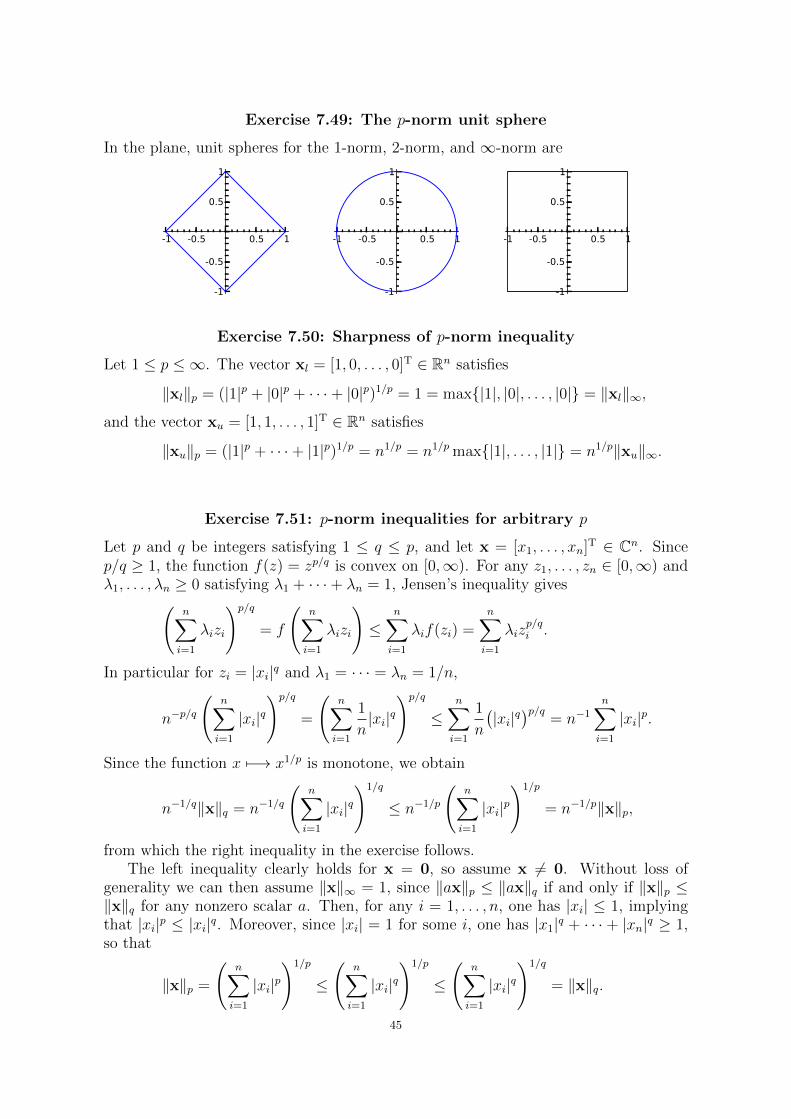
Exercise 7.49: The p-norm unit sphere

In the plane, unit spheres for the 1-norm, 2-norm, and ∞-norm are

-1 -0.5 0.5 1

-1

-0.5

0.5

1

-1 -0.5 0.5 1

-1

-0.5

0.5

1

-1 -0.5 0.5 1

-1

-0.5

0.5

1

Exercise 7.50: Sharpness of p-norm inequality

Let 1 ≤ p ≤ ∞. The vector xl = [1, 0, . . . , 0]T ∈ Rn satisfies

‖xl‖p = (|1|p + |0|p + · · ·+ |0|p)1/p = 1 = max|1|, |0|, . . . , |0| = ‖xl‖∞,

and the vector xu = [1, 1, . . . , 1]T ∈ Rn satisfies

‖xu‖p = (|1|p + · · ·+ |1|p)1/p = n1/p = n1/p max|1|, . . . , |1| = n1/p‖xu‖∞.

Exercise 7.51: p-norm inequalities for arbitrary p

Let p and q be integers satisfying 1 ≤ q ≤ p, and let x = [x1, . . . , xn]T ∈ Cn. Sincep/q ≥ 1, the function f(z) = zp/q is convex on [0,∞). For any z1, . . . , zn ∈ [0,∞) andλ1, . . . , λn ≥ 0 satisfying λ1 + · · ·+ λn = 1, Jensen’s inequality gives(

n∑i=1

λizi

)p/q

= f

(n∑i=1

λizi

)≤

n∑i=1

λif(zi) =n∑i=1

λizp/qi .

In particular for zi = |xi|q and λ1 = · · · = λn = 1/n,

n−p/q

(n∑i=1

|xi|q)p/q

=

(n∑i=1

1

n|xi|q

)p/q

≤n∑i=1

1

n

(|xi|q

)p/q= n−1

n∑i=1

|xi|p.

Since the function x 7−→ x1/p is monotone, we obtain

n−1/q‖x‖q = n−1/q

(n∑i=1

|xi|q)1/q

≤ n−1/p

(n∑i=1

|xi|p)1/p

= n−1/p‖x‖p,

from which the right inequality in the exercise follows.The left inequality clearly holds for x = 0, so assume x 6= 0. Without loss of

generality we can then assume ‖x‖∞ = 1, since ‖ax‖p ≤ ‖ax‖q if and only if ‖x‖p ≤‖x‖q for any nonzero scalar a. Then, for any i = 1, . . . , n, one has |xi| ≤ 1, implyingthat |xi|p ≤ |xi|q. Moreover, since |xi| = 1 for some i, one has |x1|q + · · · + |xn|q ≥ 1,so that

‖x‖p =

(n∑i=1

|xi|p)1/p

≤

(n∑i=1

|xi|q)1/p

≤

(n∑i=1

|xi|q)1/q

= ‖x‖q.

45

Finally we consider the case p =∞. The statement is obvious for q = p, so assumethat q is an integer. Then

‖x‖q =

(n∑i=1

|xi|q)1/q

≤

(n∑i=1

‖x‖q∞

)1/q

= n1/q‖x‖∞,

proving the right inequality. Using that the map x 7−→ x1/q is monotone, the leftinequality follows from

‖x‖q∞ = (maxi|xi|)q ≤

n∑i=1

|xi|q = ‖x‖qq.

46

CHAPTER 8

Least Squares

Exercise 8.10: Fitting a circle to points

We are given the (in general overdetermined) system

(ti − c1)2 + (yi − c2)2 = r2, i = 1, . . . ,m.

(a) Let c1 = x1/2, c2 = x2/2, and r2 = x3 + c21 + c22 as in the Exercise. Then, fori = 1, . . . ,m,

0 = (ti − c1)2 + (yi − c2)2 − r2

=(ti −

x12

)2+(yi −

x22

)2− x3 −

(x12

)2−(x2

2

)2= t2i + y2i − tix1 − yix2 − x3,

from which Equation (8.5) follows immediately. Once x1, x2, and x3 are determined,we can compute

c1 =x12, c2 =

x22, r =

√1

4x21 +

1

4x22 + x3.

(b) The linear least square problem is to minimize ‖Ax− b‖22, with

A =

t1 y1 1...

......

tm ym 1

, b =

t21 + y21...

t2m + y2m

, x =

x1x2x3

.(c) Whether or not A has independent columns depends on the data ti, yi. For

instance, if ti = yi = 1 for all i, then the columns of A are clearly dependent. Ingeneral, A has independent columns whenever we can find three points (ti, yi) not ona straight line.

(d) For these points the matrix A becomes

A =

1 4 13 2 11 0 1

,which clearly is invertible. We find

x =

x1x2x3

=

1 4 13 2 11 0 1

−1 17131

=

24−1

.It follows that c1 = 1, c2 = 2, and r = 2. The points (t, y) = (1, 4), (3, 2), (1, 0)therefore all lie on the circle

(t− 1)2 + (y − 2)2 = 4,

as shown in the following picture.

47

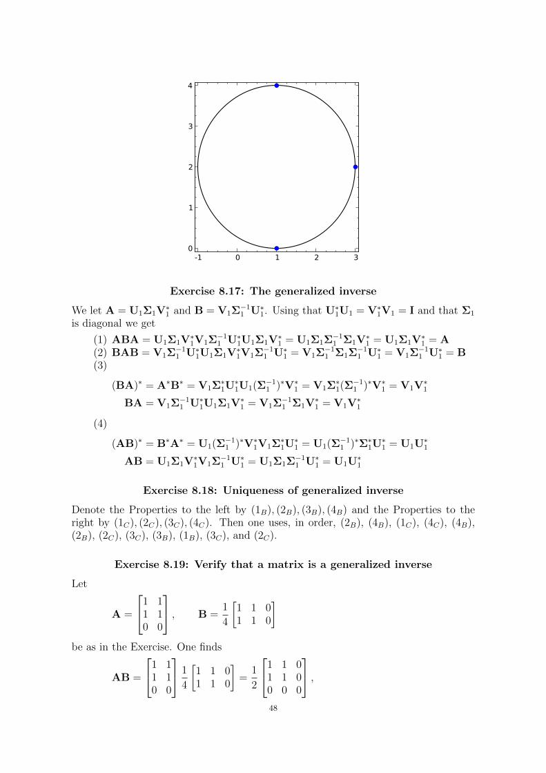
-1 0 1 2 30

1

2

3

4

Exercise 8.17: The generalized inverse

We let A = U1Σ1V∗1 and B = V1Σ

−11 U∗1. Using that U∗1U1 = V∗1V1 = I and that Σ1

is diagonal we get

(1) ABA = U1Σ1V∗1V1Σ

−11 U∗1U1Σ1V

∗1 = U1Σ1Σ

−11 Σ1V

∗1 = U1Σ1V

∗1 = A

(2) BAB = V1Σ−11 U∗1U1Σ1V

∗1V1Σ

−11 U∗1 = V1Σ

−11 Σ1Σ

−11 U∗1 = V1Σ

−11 U∗1 = B

(3)

(BA)∗ = A∗B∗ = V1Σ∗1U∗1U1(Σ

−11 )∗V∗1 = V1Σ

∗1(Σ

−11 )∗V∗1 = V1V

∗1

BA = V1Σ−11 U∗1U1Σ1V

∗1 = V1Σ

−11 Σ1V

∗1 = V1V

∗1

(4)

(AB)∗ = B∗A∗ = U1(Σ−11 )∗V∗1V1Σ

∗1U∗1 = U1(Σ

−11 )∗Σ∗1U

∗1 = U1U

∗1

AB = U1Σ1V∗1V1Σ

−11 U∗1 = U1Σ1Σ

−11 U∗1 = U1U

∗1

Exercise 8.18: Uniqueness of generalized inverse

Denote the Properties to the left by (1B), (2B), (3B), (4B) and the Properties to theright by (1C), (2C), (3C), (4C). Then one uses, in order, (2B), (4B), (1C), (4C), (4B),(2B), (2C), (3C), (3B), (1B), (3C), and (2C).

Exercise 8.19: Verify that a matrix is a generalized inverse

Let

A =

1 11 10 0

, B =1

4

[1 1 01 1 0

]be as in the Exercise. One finds

AB =

1 11 10 0

1

4

[1 1 01 1 0

]=

1

2

1 1 01 1 00 0 0

,48

BA =1

4

[1 1 01 1 0

]1 11 10 0

=1

2

[1 11 1

],

so that (AB)∗ = AB and (BA)∗ = BA. Moreover,

ABA = A(BA) =

1 11 10 0

1

2

[1 11 1

]=

1 11 10 0

= A,

BAB = (BA)B =1

2

[1 11 1

]1

4

[1 1 01 1 0

]=

1

4

[1 1 01 1 0

]= B.

By Exercises 8.17 and 8.18, we conclude that B must be the pseudoinverse of A.

Exercise 8.20: Linearly independent columns and generalized inverse

If A ∈ Cm,n has independent columns then both A and A∗ have rank n ≤ m. Then,by Exercise 6.17, A∗A must have rank n as well. Since A∗A is an n × n-matrix ofmaximal rank, it is nonsingular and we can define B := (A∗A)−1A∗. We verify thatB satisfies the four axioms of Exercise 8.17.

(1) ABA = A(A∗A)−1A∗A = A(2) BAB = (A∗A)−1A∗A(A∗A)−1A∗ = (A∗A)−1A∗ = B(3) (BA)∗ =

((A∗A)−1A∗A

)∗= I∗n = In = (A∗A)−1A∗A = BA

(4) (AB)∗ =(A(A∗A)−1A∗

)∗= A

((A∗A)−1

)∗A∗

= A(A∗A)−1A∗ = AB

It follows that B = A†. The second claim follows similarly.Alternatively, one can use the fact that the unique solution of the least squares

problem is A†b and compare this with the solution of the normal equation.

Exercise 8.21: The generalized inverse of a vector

This is a special case of Exercise 8.20. In particular, if u is a nonzero vector, thenu∗u = 〈u,u〉 = ‖u‖2 is a nonzero number and (u∗u)−1u∗ is defined. One can againcheck the axioms of Exercise 8.17 to show that this vector must be the pseudoinverseof u∗.

Exercise 8.22: The generalized inverse of an outer product

Let A = uv∗ be as in the Exercise. Since u and v are nonzero,

A = U1Σ1V∗1 =

u

‖u‖2[‖u‖2‖v‖2

] v∗

‖v‖2is a singular value factorization of A. But then

A† = V1Σ−11 U∗1 =

v

‖v‖2

[1

‖u‖2‖v‖2

] u∗

‖u‖2=

1

‖u‖22‖v‖22vu∗ =

A∗

α.

49

Exercise 8.23: The generalized inverse of a diagonal matrix

Let A := diag(λ1, . . . , λn) and B := diag(λ†1, . . . , λ†n) as in the exercise. Note that,

by definition, λ†j indeed represents the pseudoinverse of the number λj for any j. Ittherefore satisfies the axioms of Exercise 8.17, something we shall use below. We nowverify the axioms for B to show that B must be the pseudoinverse of A.

(1) ABA = diag(λ1λ†1λ1, . . . , λnλ

†nλn) = diag(λ1, . . . , λn) = A;

(2) BAB = diag(λ†1λ1λ†1, . . . , λ

†nλnλ

†n) = diag(λ†1, . . . , λ

†n) = B;

(3) (BA)∗ = (diag(λ†1λ1, . . . , λ†nλn))∗ = diag(λ†1λ1, . . . , λ

†nλn) = BA;

(4) (AB)∗ = (diag(λ1λ†1, . . . , λnλ

†n))∗ = diag(λ1λ

†1, . . . , λnλ

†n) = AB.

This proves that B is the pseudoinverse of A.

Exercise 8.24: Properties of the generalized inverse

Let A = UΣV∗ be a singular value decomposition of A and A = U1Σ1V∗1 the cor-

responding singular value factorization. By definition of the pseudo inverse, A† :=V1Σ

−11 U∗1.

(a) One has (A†)∗ = (V1Σ−11 U∗1)

∗ = U1Σ−∗1 V∗1. On the other hand, the matrix A∗

has singular value factorization A∗ = V1Σ∗1U∗1, so that its pseudo inverse is (A∗)† :=

U1Σ−∗1 V∗1 as well. We conclude that (A†)∗ = (A∗)†.

(b) Since A† := V1Σ−11 U∗1 is a singular value factorization, it has pseudo inverse

(A†)† = (U∗1)∗(Σ−11 )−1V∗1 = U1Σ1V

∗1 = A.

(c) Let α 6= 0. Since the matrix αA has singular value factorization U1(αΣ1)V∗1,

it has pseudo inverse

(αA)† = V1(αΣ1)−1U∗1 = α−1V1Σ

−11 U∗1 = α−1A†.

Exercise 8.25: The generalized inverse of a product

(a) From the condition that A has linearly independent columns we can deducethat n ≤ m. Similarly it follows that n ≤ k, hence n ≤ minm, k and both matriceshave maximal rank. As a consequence,

A = UAΣAV∗A =[UA,1 UA,2

] [ΣA,1

0

]V∗A = UA,1ΣA,1V

∗A

B = UBΣBV∗B = UB

[ΣB,1 0

] [VB,1 VB,2

]∗= UBΣB,1V

∗B,1,

where ΣA,1 and ΣB,1 are invertible, and VA and UB are unitary. This gives

A†A = VAΣ−1A,1U∗A,1UA,1ΣA,1V

∗A = VAΣ−1A,1ΣA,1V

∗A = VAV∗A = I

BB† = UBΣB,1V∗B,1VB,1Σ

−1B,1U

∗B = UBΣB,1Σ

−1B,1U

∗B = UBUB = I.

We know already from Exercise 8.17 that (AA†)∗ = AA† and (B†B)∗ = B†B. Wenow let E := AB and F := B†A†. Hence we want to show that E† = F. We do that

50

by showing that F satisfies the properties given in Exercise 8.17.

EFE = ABB†A†AB = AB = E

FEF = B†A†ABB†A† = B†A† = F

(FE)∗ = (B†A†AB)∗ = (B†B)∗ = B†B = B†A†AB = FE

(EF)∗ = (ABB†A†)∗ = (AA†)∗ = AA† = ABB†A† = EF

(b) Let A = u∗ and B = v, where u and v are column vectors. From exer-cises 8.21and 8.22 we have that A† = u/‖u‖22, and B† = v∗/‖v‖22. We have that

(AB)† = (u∗v)† = 1/(u∗v) B†A† = v∗u/(‖v‖22‖u‖22).If these are to be equal we must have that (u∗v)2 = ‖v‖22‖u‖22. We must thus haveequality in the triangle inequality, and this can happen only if u and v are paral-lel. It is thus enough to find u and v which are not parallel, in order to produce acounterexample.

Exercise 8.26: The generalized inverse of the conjugate transpose

Let A have singular value factorization A = U1Σ1V∗1, so that A∗ = V1Σ

∗1U∗1 and

A† = V1Σ−11 U∗1. Then A∗ = A† if and only if Σ∗1 = Σ−11 , which happens precisely

when all nonzero singular values of A are one.

Exercise 8.27: Linearly independent columns

By Exercise 8.20, if A has rank n, then A† = (A∗A)−1A∗. Then A(A∗A)−1A∗b =AA†b, which is the orthogonal projection of b into span(A) by Theorem 8.12.

Exercise 8.28: Analysis of the general linear system

In this exercise, we can write

Σ =

[Σ1 00 0

], Σ1 = diag(σ1, . . . , σr), σ1 > · · · > σr > 0.

(a) As U is unitary, we have U∗U = I. We find the following sequence of equiva-lences.

Ax = b ⇐⇒ UΣV∗x = b ⇐⇒ U∗UΣ(V∗x) = U∗b ⇐⇒ Σy = c,

which is what needed to be shown.(b) By (a), the linear system Ax = b has a solution if and only if the system

[Σ1 00 0

]y =

σ1y1...

σryr0...0

=

c1...crcr+1

...cn

= c

has a solution y. Since σ1, . . . , σr 6= 0, this system has a solution if and only ifcr+1 = · · · = cn = 0. We conclude that Ax = b has a solution if and only if cr+1 =· · · = cn = 0.

(c) By (a), the linear system Ax = b has a solution if and only if the systemΣy = c has a solution. Hence we have the following three cases.

51

r = n:Here yi = ci/σi for i = 1, . . . , n provides the only solution to the systemΣy = b, and therefore x = Vy is the only solution to Ax = b. It follows thatthe system has exactly one solution.

r < n, ci = 0 for i = r + 1, . . . , n:Here each solution y must satisfy yi = ci/σi for i = 1, . . . , r. The remainingyr+1, . . . , yn, however, can be chosen arbitrarily. Hence we have infinitely manysolutions to Σy = b as well as for Ax = b.

r < n, ci 6= 0 for some i with r + 1 ≤ i ≤ n:In this case it is impossible to find a y that satisfies Σy = b, and thereforethe system Ax = b has no solution at all.

Exercise 8.29: Fredholm’s Alternative

Suppose that the system Ax = b has a solution, i.e., b ∈ span(A). Suppose inaddition that A∗y = 0 has a solution, i.e., y ∈ ker(A∗). Since (span(A))⊥ = ker(A∗),one has 〈y,b〉 = y∗b = 0. Thus if the system Ax = b has a solution, then we cannot find a solution to A∗y = 0, y∗b 6= 0. Conversely if y ∈ ker(A∗) and y∗b 6= 0,then b /∈ (ker(A∗))⊥ = span(A), implying that the system Ax = b does not have asolution.

Exercise 8.32: Condition number

Let

A =

1 21 11 1

, b =

b1b2b3

be as in the Exercise.

(a) By Exercise 8.20, the pseudoinverse of A is

A† = (ATA)−1AT =

[−1 1 11 −1

2−1

2

].

Theorem 8.12 tells us that the orthogonal projection of b into span(A) is

b1 := AA†b =

1 0 00 1

212

0 12

12

b1b2b3

=1

2

2b1b2 + b3b2 + b3

,so that the orthogonal projection of b into ker(AT) is

b2 := (I−AA†)b =

0 0 00 1

2−1

20 −1

212

b1b2b3

=1

2

0b2 − b3b3 − b2

,where we used that b = b1 + b2.

(b) By Theorem 7.15, the 2-norms ‖A‖2 and ‖A†‖2 can be found by computing thelargest singular values of the matrices A and A†. The largest singular value σ1 of A isthe square root of the largest eigenvalue λ1 of ATA, which satisfies

0 = det(ATA− λ1I) = det

[3− λ1 4

4 6− λ1

]= λ21 − 9λ1 + 2.

52

It follows that σ1 = 12

√2√

9 +√

73. Similarly, the largest singular value σ2 of A† is

the square root of the largest eigenvalue λ2 of A†TA†, which satisfies

0 = det(A†TA† − λ2I) = det

1

4

8 −6 −6−6 5 5−6 5 5

− λ2I

= −1

2λ2(2λ22 − 9λ2 + 1

).

Alternatively, we could have used that the largest singular value of A† is the inverse ofthe smallest singular value of A (this follows from the singular value factorization). It

follows that σ2 = 12

√9 +√

73 =√

2/√

9−√

73. We conclude

K(A) = ‖A‖2 · ‖A†‖2 =

√9 +√

73

9−√

73=

1

2√

2

(9 +√

73)≈ 6.203.

Exercise 8.35: Problem using normal equations

(a) Let A, b, and ε be as in the exercise. The normal equations ATAx = ATb arethen [

3 3 + ε3 + ε (ε+ 1)2 + 2

] [x1x2

]=

[7

7 + 2ε

].

If ε 6= 0, inverting the matrix ATA yields the unique solution[x1x2

]=

1

2ε2

[(ε+ 1)2 + 2 −3− ε−3− ε 3

] [7

7 + 2ε

]=

[52

+ 12ε

− 12ε

].

If ε = 0, on the other hand, then any vector x = [x1, x2]T with x1 + x2 = 7/3 is a

solution.(b) For ε = 0, we get the same solution as in (a). For ε 6= 0, however, the solution

to the system[3 3 + ε

3 + ε 3 + 2ε

] [x1x2

]=

[7

7 + 2ε

]is [

x′1x′2

]= − 1

ε2

[3 + 2ε −3− ε−3− ε 3

] [7

7 + 2ε

]=

[2− 1

ε1ε

].

We can compare this to the solution of (a) by comparing the residuals,∣∣∣∣∣∣∣∣A [52

+ 12ε

− 12ε

]− b

∣∣∣∣∣∣∣∣2

=

∣∣∣∣∣∣∣∣∣∣∣∣ 1

2−1

20

∣∣∣∣∣∣∣∣∣∣∣∣2

=1√2

≤√

2 =

∣∣∣∣∣∣∣∣∣∣∣∣ 0−11

∣∣∣∣∣∣∣∣∣∣∣∣2

=

∣∣∣∣∣∣∣∣A [2− 1ε

1ε

]− b

∣∣∣∣∣∣∣∣2

,

which shows that the solution from (a) is more accurate.

53

CHAPTER 9

The Kronecker Product

Exercise 9.2: 2× 2 Poisson matrix

For m = 2, the Poisson matrix A is the 22 × 22 matrix given by4 −1 −1 0−1 4 0 −1−1 0 4 −1

0 −1 −1 4

.In every row i, one has |aii| = 4 > 2 = | − 1|+ | − 1|+ |0| =

∑j 6=i |aij|. In other words,

A is strictly diagonally dominant.

Exercise 9.5: Properties of Kronecker products

Let be given matrices A,A1,A2 ∈ Rp×q, B,B1,B2 ∈ Rr×s, and C ∈ Rt×u. Then(λA)⊗ (µB) = λµ(A⊗B) by definition of the Kronecker product and since

(λA)µb11 (λA)µb12 · · · (λA)µb1s(λA)µb21 (λA)µb22 · · · (λA)µb2s

......

. . ....

(λA)µbr1 (λA)µbr2 · · · (λA)µbrs

= λµ

Ab11 Ab12 · · · Ab1sAb21 Ab22 · · · Ab2s

......

. . ....

Abr1 Abr2 · · · Abrs

.The identity (A1 + A2)⊗B = (A1 ⊗B) + (A2 ⊗B) follows from

(A1 + A2)b11 (A1 + A2)b12 · · · (A1 + A2)b1s(A1 + A2)b21 (A1 + A2)b22 · · · (A1 + A2)b2s

......

. . ....

(A1 + A2)br1 (A1 + A2)br2 · · · (A1 + A2)brs

=

A1b11 + A2b11 A1b12 + A2b12 · · · A1b1s + A2b1sA1b21 + A2b21 A1b22 + A2b22 · · · A1b2s + A2b2s

......

. . ....

A1br1 + A2br1 A1br2 + A2br2 · · · A1brs + A2brs

=

A1b11 A1b12 · · · A1b1sA1b21 A1b22 · · · A1b2s

......

. . ....

A1br1 A1br2 · · · A1brs

+

A2b11 A2b12 · · · A2b1sA2b21 A2b22 · · · A2b2s

......

. . ....

A2br1 A2br2 · · · A2brs

.A similar argument proves A⊗ (B1 + B2) = (A⊗B1) + (A⊗B2), and therefore thebilinearity of the Kronecker product. The associativity (A⊗B)⊗C = A⊗ (B⊗C)

54

follows from

=

Ab11 · · · Ab1s...

...Abr1 · · · Abrs

⊗C

=

Ab11c11 · · · Ab1sc11 Ab11c1u · · · Ab1sc1u...

... · · · ......

Abr1c11 · · · Abrsc11 Abr1c1u · · · Abrsc1u...

...Ab11ct1 · · · Ab1sct1 Ab11ctu · · · Ab1sctu

...... · · · ...

...Abr1ct1 · · · Abrsct1 Abr1ctu · · · Abrsctu

= A⊗

b11c11 · · · b1sc11 b11c1u · · · b1sc1u...

... · · · ......

br1c11 · · · brsc11 br1c1u · · · brsc1u...

...b11ct1 · · · b1sct1 b11ctu · · · b1sctu

...... · · · ...

...br1ct1 · · · brsct1 br1ctu · · · brsctu

= A⊗

Bc11 · · · Bc1u...

...Bct1 · · · Bctu

.Exercise 9.9: 2nd derivative matrix is positive definite

Applying Lemma 1.31 to the case that a = −1 and d = 2, one finds that the eigenvaluesλj of the matrix tridiag(−1, 2,−1) ∈ Rm,m are

λj = d+ 2a cos

(jπ

m+ 1

)= 2

(1− cos

(jπ

m+ 1

)),

for j = 1, . . . ,m. Moreover, as |cos(x)| < 1 for any x ∈ (0, π), it follows that λj > 0 forj = 1, . . . ,m. Since, in addition, tridiag(−1, 2,−1) is symmetric, Lemma 3.16 impliesthat the matrix tridiag(−1, 2,−1) is symmetric positive definite.

Exercise 9.10: 1D test matrix is positive definite?

The statement of this exercise is a generalization of the statement of Exercise 9.9.Consider a matrix M = tridiag(a, d, a) ∈ Rm,m for which d > 0 and d ≥ 2|a|. ByLemma 1.31, the eigenvalues λj, with j = 1, . . . ,m, of the matrix M are

λj = d+ 2a cos

(jπ

m+ 1

).

If a = 0, then all these eigenvalues are equal to d and therefore positive. If a 6= 0, writesgn(a) for the sign of a. Then

λj ≥ 2|a|[1 +

a

|a|cos

(jπ

m+ 1

)]= 2|a|

[1 + sgn(a) cos

(jπ

m+ 1

)]> 0,

55

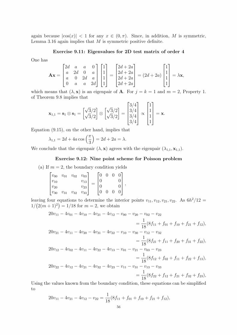
again because |cos(x)| < 1 for any x ∈ (0, π). Since, in addition, M is symmetric,Lemma 3.16 again implies that M is symmetric positive definite.

Exercise 9.11: Eigenvalues for 2D test matrix of order 4

One has

Ax =

2d a a 0a 2d 0 aa 0 2d a0 a a 2d

1111

=

2d+ 2a2d+ 2a2d+ 2a2d+ 2a

= (2d+ 2a)

1111

= λx,

which means that (λ,x) is an eigenpair of A. For j = k = 1 and m = 2, Property 1.of Theorem 9.8 implies that

x1,1 = s1 ⊗ s1 =

[√3/2√3/2

]⊗[√

3/2√3/2

]=

3/43/43/43/4

∝

1111

= x.

Equation (9.15), on the other hand, implies that

λ1,1 = 2d+ 4a cos(π

3

)= 2d+ 2a = λ.

We conclude that the eigenpair (λ,x) agrees with the eigenpair (λ1,1,x1,1).

Exercise 9.12: Nine point scheme for Poisson problem

(a) If m = 2, the boundary condition yieldsv00 v01 v02 v03v10 v13v20 v23v30 v31 v32 v33

=

0 0 0 00 00 00 0 0 0

,leaving four equations to determine the interior points v11, v12, v21, v22. As 6h2/12 =1/(2(m+ 1)2

)= 1/18 for m = 2, we obtain

20v11 − 4v01 − 4v10 − 4v21 − 4v12 − v00 − v20 − v02 − v22

=1

18(8f11 + f01 + f10 + f21 + f12),

20v21 − 4v11 − 4v20 − 4v31 − 4v22 − v10 − v30 − v12 − v32

=1

18(8f21 + f11 + f20 + f31 + f22),

20v12 − 4v02 − 4v11 − 4v22 − 4v13 − v01 − v21 − v03 − v23

=1

18(8f12 + f02 + f11 + f22 + f13),

20v22 − 4v12 − 4v21 − 4v32 − 4v23 − v11 − v31 − v13 − v33

=1

18(8f22 + f12 + f21 + f32 + f23),

Using the values known from the boundary condition, these equations can be simplifiedto

20v11 − 4v21 − 4v12 − v22 =1

18(8f11 + f01 + f10 + f21 + f12),

56

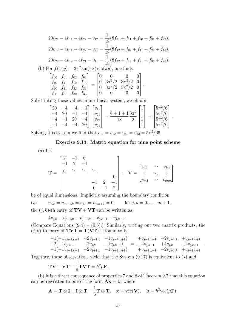
20v21 − 4v11 − 4v22 − v12 =1

18(8f21 + f11 + f20 + f31 + f22),

20v12 − 4v11 − 4v22 − v21 =1

18(8f12 + f02 + f11 + f22 + f13),

20v22 − 4v12 − 4v21 − v11 =1

18(8f22 + f12 + f21 + f32 + f23).

(b) For f(x, y) = 2π2 sin(πx) sin(πy), one findsf00 f01 f02 f03f10 f11 f12 f13f20 f21 f22 f23f30 f31 f32 f33

=

0 0 0 00 3π2/2 3π2/2 00 3π2/2 3π2/2 00 0 0 0

.Substituting these values in our linear system, we obtain

20 −4 −4 −1−4 20 −1 −4−4 −1 20 −4−1 −4 −4 20

v11v21v12v22

=8 + 1 + 1

18

3π2

2

1111

=

5π2/65π2/65π2/65π2/6

.Solving this system we find that v11 = v12 = v21 = v22 = 5π2/66.

Exercise 9.13: Matrix equation for nine point scheme

(a) Let

T =

2 −1 0−1 2 −1

0. . . . . . . . .

0−1 2 −10 −1 2

, V =

v11 · · · v1m...

. . ....

vm1 · · · vmm

be of equal dimensions. Implicitly assuming the boundary condition

(?) v0,k = vm+1,k = vj,0 = vj,m+1 = 0, for j, k = 0, . . . ,m+ 1,

the (j, k)-th entry of TV + VT can be written as

4vj,k − vj−1,k − vj+1,k − vj,k−1 − vj,k+1.

(Compare Equations (9.4) – (9.5).) Similarly, writing out two matrix products, the(j, k)-th entry of TVT = T(VT) is found to be

−1(−1vj−1,k−1 +2vj−1,k −1vj−1,k+1)+2(−1vj,k−1 +2vj,k −1vj,k+1)−1(−1vj+1,k−1 +2vj+1,k −1vj+1,k+1)

=+vj−1,k−1 −2vj−1,k +vj−1,k+1

−2vj,k−1 +4vj,k −2vj,k+1

+vj+1,k−1 −2vj+1,k +vj+1,k+1

.

Together, these observations yield that the System (9.17) is equivalent to (?) and

TV + VT− 1

6TVT = h2µF.

(b) It is a direct consequence of properties 7 and 8 of Theorem 9.7 that this equationcan be rewritten to one of the form Ax = b, where

A = T⊗ I + I⊗T− 1

6T⊗T, x = vec(V), b = h2vec(µF).

57

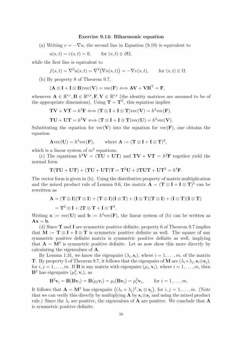
Exercise 9.14: Biharmonic equation

(a) Writing v = −∇u, the second line in Equation (9.19) is equivalent to

u(s, t) = v(s, t) = 0, for (s, t) ∈ ∂Ω,

while the first line is equivalent to

f(s, t) = ∇2u(s, t) = ∇2(∇u(s, t)

)= −∇v(s, t), for (s, t) ∈ Ω.

(b) By property 8 of Theorem 9.7,

(A⊗ I + I⊗B)vec(V) = vec(F)⇐⇒ AV + VBT = F,

whenever A ∈ Rr,r,B ∈ Rs,s,F,V ∈ Rr,s (the identity matrices are assumed to be ofthe appropriate dimensions). Using T = TT, this equation implies

TV + VT = h2F⇐⇒ (T⊗ I + I⊗T)vec(V) = h2vec(F),

TU + UT = h2V⇐⇒ (T⊗ I + I⊗T)vec(U) = h2vec(V).

Substituting the equation for vec(V) into the equation for vec(F), one obtains theequation

Avec(U) = h4vec(F), where A := (T⊗ I + I⊗T)2,

which is a linear system of m2 equations.(c) The equations h2V = (TU + UT) and TV + VT = h2F together yield the

normal form

T(TU + UT) + (TU + UT)T = T2U + 2TUT + UT2 = h4F.

The vector form is given in (b). Using the distributive property of matrix multiplicationand the mixed product rule of Lemma 9.6, the matrix A = (T ⊗ I + I ⊗ T)2 can berewritten as

A = (T⊗ I)(T⊗ I) + (T⊗ I)(I⊗T) + (I⊗T)(T⊗ I) + (I⊗T)(I⊗T)

= T2 ⊗ I + 2T⊗T + I⊗T2.

Writing x := vec(U) and b := h4vec(F), the linear system of (b) can be written asAx = b.

(d) Since T and I are symmetric positive definite, property 6 of Theorem 9.7 impliesthat M := T ⊗ I + I ⊗ T is symmetric positive definite as well. The square of anysymmetric positive definite matrix is symmetric positive definite as well, implyingthat A = M2 is symmetric positive definite. Let us now show this more directly bycalculating the eigenvalues of A.

By Lemma 1.31, we know the eigenpairs (λi, si), where i = 1, . . . ,m, of the matrixT. By property 5 of Theorem 9.7, it follows that the eigenpairs of M are (λi+λj, si⊗sj),for i, j = 1, . . . ,m. If B is any matrix with eigenpairs (µi,vi), where i = 1, . . . ,m, thenB2 has eigenpairs (µ2

i ,vi), as

B2vi = B(Bvi) = B(µivi) = µi(Bvi) = µ2ivi, for i = 1, . . . ,m.

It follows that A = M2 has eigenpairs((λi + λj)

2, si ⊗ sj), for i, j = 1, . . . ,m. (Note

that we can verify this directly by multiplying A by si⊗sj and using the mixed productrule.) Since the λi are positive, the eigenvalues of A are positive. We conclude that Ais symmetric positive definite.

58

Writing A = T2 ⊗ I + 2T⊗T + I⊗T2 and computing the block structure of eachof these terms, one finds that A has bandwidth 2m, in the sense that any row has atmost 4m+ 1 nonzero elements.

(e) One can expect to solve the system of (b) faster, as it is typically quicker tosolve two simple systems instead of one complex system.

59

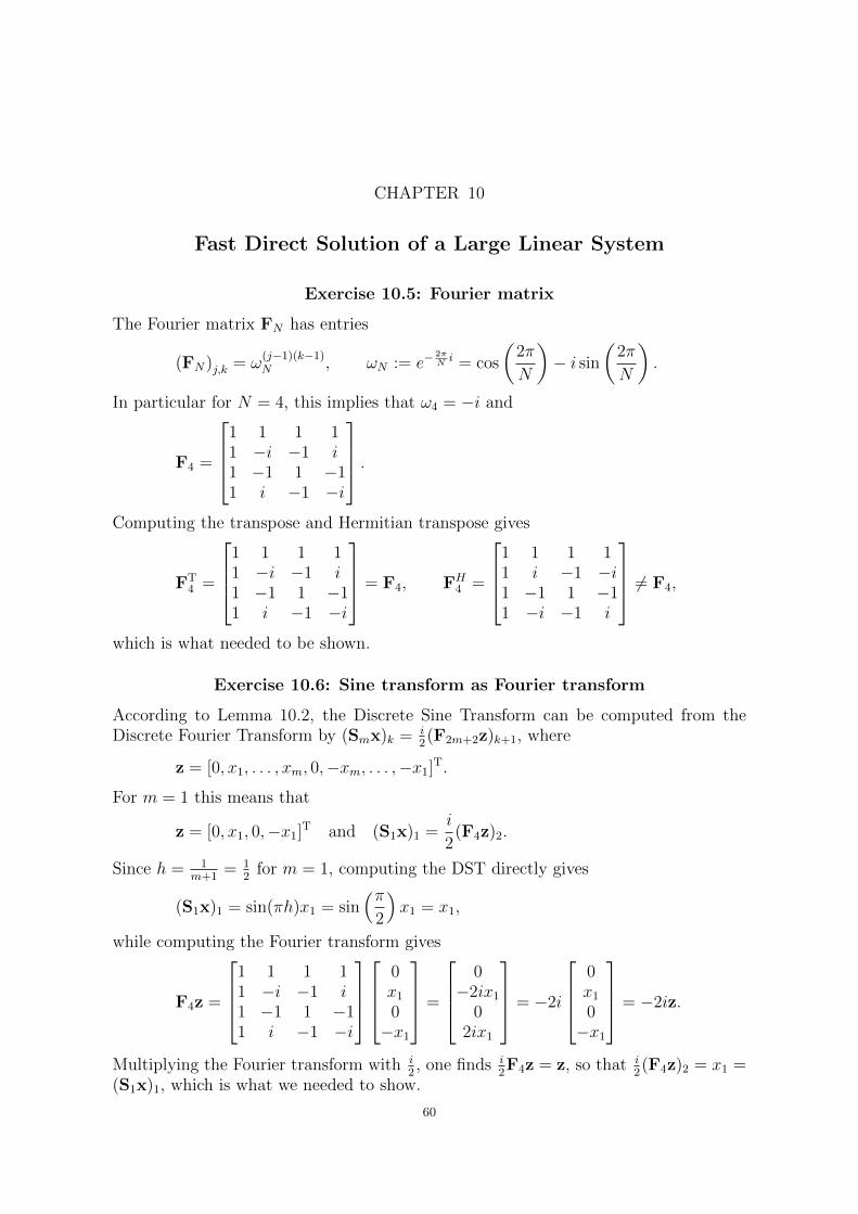
CHAPTER 10

Fast Direct Solution of a Large Linear System

Exercise 10.5: Fourier matrix

The Fourier matrix FN has entries

(FN)j,k = ω(j−1)(k−1)N , ωN := e−

2πNi = cos

(2π

N

)− i sin

(2π

N

).

In particular for N = 4, this implies that ω4 = −i and

F4 =

1 1 1 11 −i −1 i1 −1 1 −11 i −1 −i

.Computing the transpose and Hermitian transpose gives

FT4 =

1 1 1 11 −i −1 i1 −1 1 −11 i −1 −i

= F4, FH4 =

1 1 1 11 i −1 −i1 −1 1 −11 −i −1 i

6= F4,


Exercise 10.6: Sine transform as Fourier transform

According to Lemma 10.2, the Discrete Sine Transform can be computed from theDiscrete Fourier Transform by (Smx)k = i

2(F2m+2z)k+1, where

z = [0, x1, . . . , xm, 0,−xm, . . . ,−x1]T.

For m = 1 this means that

z = [0, x1, 0,−x1]T and (S1x)1 =i

2(F4z)2.

Since h = 1m+1

= 12

for m = 1, computing the DST directly gives

(S1x)1 = sin(πh)x1 = sin(π

2

)x1 = x1,

while computing the Fourier transform gives

F4z =

1 1 1 11 −i −1 i1 −1 1 −11 i −1 −i

0x10−x1

=

0

−2ix10

2ix1

= −2i

0x10−x1

= −2iz.

Multiplying the Fourier transform with i2, one finds i

2F4z = z, so that i

2(F4z)2 = x1 =

(S1x)1, which is what we needed to show.

60

Exercise 10.7: Explicit solution of the discrete Poisson equation

For any integer m ≥ 1, let h = 1/(m + 1). For j = 1, . . . ,m, let λj = 4 sin2(jπh/2

),

D = diag(λ1, . . . , λm), and S = (sjk)jk =(

sin(jkπh))jk

. By Section 10.2, the solution

to the discrete Poisson equation is V = SXS, where X is found by solving DX+XD =4h4SFS. Since D is diagonal, one has (DX + XD)pr = (λp + λr)xpr, so that

xpr = 4h4(SFS)prλp + λr

= 4h4m∑k=1

m∑l=1

spkfklslrλp + λr

so that

vij =m∑p=1

m∑r=1

sipxprsrj = 4h4m∑p=1

m∑r=1

m∑k=1

m∑l=1

sipspkslrsrjλp + λr

fkl

= h4m∑p=1

m∑r=1

m∑k=1

m∑l=1

sin(ipπm+1

)sin(pkπm+1

)sin(lrπm+1

)sin(rjπm+1

)sin2

(pπ

2(m+1)

)+ sin2

(rπ

2(m+1)

) fkl,


Exercise 10.8: Improved version of Algorithm 10.1

Given is that

(?) TV + VT = h2F.

Let T = SDS−1 be the orthogonal diagonalization of T from Equation (10.4), andwrite X = VS and C = h2FS.

(a) Multiplying Equation (?) from the right by S, one obtains

TX + XD = TVS + VSD = TVS + VTS = h2FS = C.

(b) Writing C = [c1, . . . , cm], X = [x1, . . . ,xm] and applying the rules of blockmultiplication, we find

[c1, . . . , cm] = C

= TX + XD

= T[x1, . . . ,xm] + X[λ1e1, . . . , λmem]

= [Tx1 + λ1Xe1, . . . ,Txm + λmXem]

= [Tx1 + λ1x1, . . . ,Txm + λmxm]

= [(T + λ1I)x1, . . . , (T + λmI)xm],

which is equivalent to System (10.9). To find X, we therefore need to solve the mtridiagonal linear systems of (10.9). Since the eigenvalues λ1, . . . , λm are positive,each matrix T + λjI is diagonally dominant. By Theorem 1.24, every such matrixis nonsingular and has a unique LU factorization. Algorithms 1.8 and 1.9 then solvethe corresponding system (T + λjI)xj = cj in O(δm) operations for some constant δ.Doing this for all m columns x1, . . . ,xm, one finds the matrix X in O(δm2) operations.

(c) To find V, we first find C = h2FS by performing O(2m3) operations. Next wefind X as in step b) by performing O(δm2) operations. Finally we compute V = 2hXSby performing O(2m3) operations. In total, this amounts to O(4m3) operations.

61

(d) As explained in Section 10.3, multiplying by the matrix S can be done inO(2m2 log2m) operations by using the Fourier transform. The two matrix multiplica-tions in c) can therefore be carried out in

O(4γm2 log2m) = O(4γn log2 n1/2) = O(2γn log2 n)

operations.

Exercise 10.9: Fast solution of 9 point scheme

Analogously to Section 10.2, we use the relations between the matrices T,S,X,D torewrite Equation (9.18).

TV + VT− 1

6TVT = h2µF

⇐⇒ TSXS + SXST− 1

6TSXST = h2µF

⇐⇒ STSXS2 + S2XSTS− 1

6STSXSTS = h2µSFS

⇐⇒ S2DXS2 + S2XS2D− 1

6S2DXS2D = h2µSFS

⇐⇒ DX + XD− 1

6DXD = 4h4µSFS = 4h4G

Writing D = diag(λ1, . . . , λm), the (j, k)-th entry of DX + XD − 16DXD is equal to

λjxjk + xjkλk − 16λjxjkλk. Isolating xjk and writing λj = 4σj = 4 sin2(jπh/2) then

yields

xjk =4h4gjk

λj + λk − 16λjλk

=h4gjk

σj + σk − 23σjσk

, σj = sin2

(jπh

2

).

Defining α := jπh/2 and β = kπh/2, one has 0 < α, β < π/2. Note that

σj + σk −2

3σjσk > σj + σk − σjσk

= 2− cos2 α− cos2 β − (1− cos2 α)(1− cos2 β)

= 1− cos2 α cos2 β

≥ 1− cos2 β

≥ 0.

Let A = T ⊗ I + I ⊗ T − 16T ⊗ T be as in Exercise 9.13.(b) and si as in Section

10.2. Applying the mixed-product rule, one obtains

A(si ⊗ sj) = (T⊗ I + I⊗T)(si ⊗ sj)−1

6(T⊗T)(si ⊗ sj) =

(λi + λj)(si ⊗ sj)−1

6λiλj(si ⊗ sj) = (λi + λj −

1

6λiλj)(si ⊗ sj).

The matrix A therefore has eigenvectors si ⊗ sj, and counting them shows that thesemust be all of them. As shown above, the corresponding eigen values λi + λj − 1

6λiλj

are positive, implying that the matrix A is positive definite. It follows that the System(9.17) always has a (unique) solution.

62

Exercise 10.10: Algorithm for fast solution of 9 point scheme

The following describes an algorithm for solving System (9.17).

Algorithm 1 A method for solving the discrete Poisson problem (9.17)

Require: An integer m denoting the grid size, a matrix µF ∈ Rm,m of function values.Ensure: The solution V to the discrete Poisson problem (9.17).1: h← 1

m+1

2: S←(

sin(jkπh))mj,k=1

3: σ ←(sin2

(jπh2

))mj=1

4: G← SµFS

5: X←(

h4gi,jσi+σj− 2

3σiσj

)mj,k=1

6: V← SXS

For the individual steps in this algorithm, the time complexities are shown in thefollowing table.

step 1 2 3 4 5 6

complexity O(1) O(m2) O(m) O(m3) O(m2) O(m3)

Hence the overall complexity is determined by the four matrix multiplications andgiven by O(m3).

Exercise 10.11: Fast solution of biharmonic equation

From Exercise 9.14 we know that T ∈ Rm×m is the second derivative matrix. Accordingto Lemma 1.31, the eigenpairs (λj, sj), with j = 1, . . . ,m, of T are given by

sj = [sin(jπh), sin(2jπh), . . . , sin(mjπh)]T,

λj = 2− 2 cos(jπh) = 4 sin2(jπh/2),

and satisfy sTj sk = δj,k/(2h) for all j, k, where h := 1/(m + 1). Using, in order, that

U = SXS, TS = SD, and S2 = I/(2h), one finds that

h4F = T2U + 2TUT + UT2

⇐⇒ h4F = T2SXS + 2TSXST + SXST2

⇐⇒ h4SFS = ST2SXS2 + 2STSXSTS + S2XST2S

⇐⇒ h4SFS = S2D2XS2 + 2S2DXS2D + S2XS2D2

⇐⇒ h4SFS = ID2XI/(4h2) + 2IDXID/(4h2) + IXID2/(4h2)

⇐⇒ 4h6G = D2X + 2DXD + XD2,

where G := SFS. The (j, k)-th entry of the latter matrix equation is

4h6gjk = λ2jxjk + 2λjxjkλk + xjkλ2k = xjk(λj + λk)

2.

Writing σj := sin2(jπh/2) = λj/4, one obtains

xjk =4h6gjk

(λj + λk)2=

4h6gjk(4 sin2(jπh/2) + 4 sin2(kπh/2)

)2 =h6gjk

4(σj + σk)2.

63

Exercise 10.12: Algorithm for fast solution of biharmonic equation

In order to derive an algorithm that computes U in Problem 9.14, we can adjustAlgorithm 10.1 by replacing the computation of the matrix X by the formula fromExercise 10.11. This adjustment does not change the complexity of Algorithm 10.1,which therefore remains O(δn3/2). The new algorithm can be implemented in Matlab asin Listing 10.1.

function U = simplefastbiharmonic(F)m = length(F);h = 1/(m+1);hv = pi*h*(1:m)’;sigma = sin(hv/2). 2;S = sin(hv*(1:m));G = S*F*S;X = (h 6)*G./(4*(sigma*ones(1,m)+ones(m,1)*sigma’). 2);U = zeros(m+2,m+2);U(2:m+1,2:m+1) = S*X*S;

end

Listing 10.1. A simple fast solution to the biharmonic equation

Exercise 10.13: Check algorithm for fast solution of biharmonic equation

The Matlab function from Listing 10.2 directly solves the standard form Ax = bof Equation (9.21), making sure to return a matrix of the same dimension as theimplementation from Listing 10.1.

function V = standardbiharmonic(F)m = length(F);h = 1/(m+1);T = gallery(’tridiag’, m, -1, 2,-1);A = kron(T 2, eye(m)) + 2*kron(T,T) + kron(eye(m),T 2);b = h. 4*F(:);x = A\b;V = zeros(m+2, m+2);V(2:m+1,2:m+1) = reshape(x,m,m);

end

Listing 10.2. A direct solution to the biharmonic equation

After specifying m = 4 by issuing the command F = ones(4,4), the com-mands simplefastbiharmonic(F) and standardbiharmonic(F) both returnthe matrix

0 0 0 0 0 00 0.0015 0.0024 0.0024 0.0015 00 0.0024 0.0037 0.0037 0.0024 00 0.0024 0.0037 0.0037 0.0024 00 0.0015 0.0024 0.0024 0.0015 00 0 0 0 0 0

.64

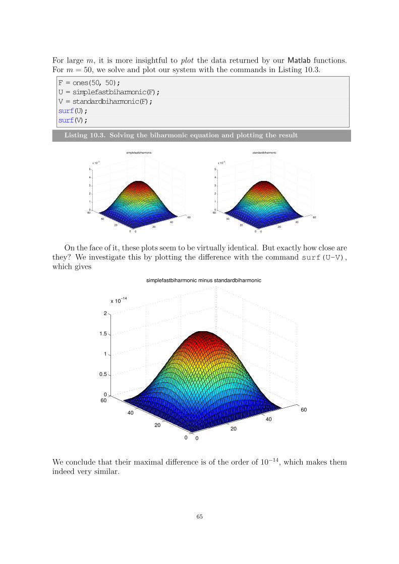
For large m, it is more insightful to plot the data returned by our Matlab functions.For m = 50, we solve and plot our system with the commands in Listing 10.3.

F = ones(50, 50);U = simplefastbiharmonic(F);V = standardbiharmonic(F);surf(U);surf(V);

Listing 10.3. Solving the biharmonic equation and plotting the result

0

20

40

60

0

20

40

600

1

2

3

4

5

x 10−3

simplefastbiharmonic

0

20

40

60

0

20

40

60

0

1

2

3

4

5

x 10−3

standardbiharmonic

On the face of it, these plots seem to be virtually identical. But exactly how close arethey? We investigate this by plotting the difference with the command surf(U-V),which gives

0

20

40

60

0

20

40

600

0.5

1

1.5

2

x 10−14

simplefastbiharmonic minus standardbiharmonic

We conclude that their maximal difference is of the order of 10−14, which makes themindeed very similar.

65

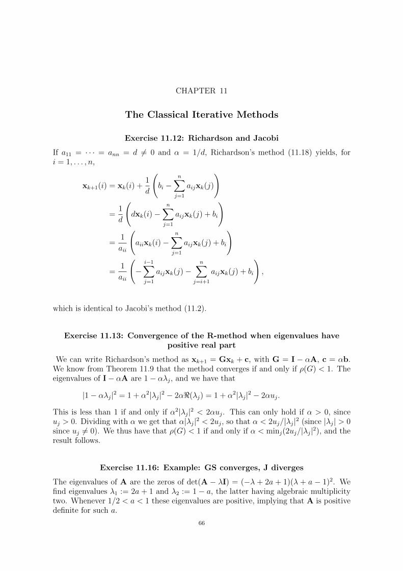
CHAPTER 11

The Classical Iterative Methods

Exercise 11.12: Richardson and Jacobi

If a11 = · · · = ann = d 6= 0 and α = 1/d, Richardson’s method (11.18) yields, fori = 1, . . . , n,

xk+1(i) = xk(i) +1

d

(bi −

n∑j=1

aijxk(j)

)

=1

d

(dxk(i)−

n∑j=1

aijxk(j) + bi

)

=1

aii

(aiixk(i)−

n∑j=1

aijxk(j) + bi

)

=1

aii

(−

i−1∑j=1

aijxk(j)−n∑

j=i+1

aijxk(j) + bi

),

which is identical to Jacobi’s method (11.2).

Exercise 11.13: Convergence of the R-method when eigenvalues havepositive real part

We can write Richardson’s method as xk+1 = Gxk + c, with G = I − αA, c = αb.We know from Theorem 11.9 that the method converges if and only if ρ(G) < 1. Theeigenvalues of I− αA are 1− αλj, and we have that

|1− αλj|2 = 1 + α2|λj|2 − 2α<(λj) = 1 + α2|λj|2 − 2αuj.

This is less than 1 if and only if α2|λj|2 < 2αuj. This can only hold if α > 0, sinceuj > 0. Dividing with α we get that α|λj|2 < 2uj, so that α < 2uj/|λj|2 (since |λj| > 0since uj 6= 0). We thus have that ρ(G) < 1 if and only if α < minj(2uj/|λj|2), and theresult follows.

Exercise 11.16: Example: GS converges, J diverges

The eigenvalues of A are the zeros of det(A − λI) = (−λ + 2a + 1)(λ + a − 1)2. Wefind eigenvalues λ1 := 2a + 1 and λ2 := 1− a, the latter having algebraic multiplicitytwo. Whenever 1/2 < a < 1 these eigenvalues are positive, implying that A is positivedefinite for such a.

66

Let’s compute the spectral radius of GJ = I−D−1A, where D is the diagonal partof A. The eigenvalues of GJ are the zeros of the characteristic polynomial

det(GJ − λI) =

∣∣∣∣∣∣−λ −a −a−a −λ −a−a −a −λ

∣∣∣∣∣∣ = (−λ− 2a)(a− λ)2,

and we find spectral radius ρ(GJ) = max|a|, |2a|. It follows that ρ(GJ) > 1 whenever1/2 < a < 1, in which case Theorem 11.9 implies that the Jacobi method does notconverge (even though A is symmetric positive definite).

Exercise 11.17: Divergence example for J and GS

We compute the matrices GJ and G1 from A and show that that the spectral radiiρ(GJ), ρ(G1) ≥ 1. Once this is shown, Theorem 11.9 implies that the Jacobi methodand Gauss-Seidel’s method diverge.

Write A = D−AL −AR as in the book. From Equation (11.12), we find

GJ = I−M−1J A = I−D−1A =

[1 00 1

]−[1 00 1

4

] [1 23 4

]=

[0 −2−3

40

],

G1 = I−M−11 A = I− (D−AL)−1A =

[1 00 1

]−[

1 0−3

414

] [1 23 4

]

=

[0 −20 3

2

].

From this, we find ρ(GJ) =√

3/2 and ρ(G1) = 3/2, both of which are bigger than 1.

Exercise 11.18: Strictly diagonally dominance; The J method

If A = (aij)ij is strictly diagonally dominant, then it is nonsingular and a11, . . . , ann 6=0. For the Jacobi method, one finds

G = I− diag(a11, . . . , ann)−1A =

0 −a12

a11−a13a11

· · · −a1na11

−a21a22

0 −a23a22

· · · −a2na22

−a31a33

−a32a33

0 · · · −a3na33

......

.... . .

...− an1ann

− an2ann

− an3ann

· · · 0

.

By Theorem 7.15, the ∞-norm can be expressed as the maximum, over all rows, ofthe sum of absolute values of the entries in a row. Using that A is strictly diagonallydominant, one finds

‖G‖∞ = maxi

∑j 6=i

∣∣∣∣−aijaii∣∣∣∣ = max

1≤i≤n

∑j 6=i |aij||aii|

< 1.

As by Lemma 7.14 the ∞-norm is consistent, Corollary 11.8 implies that the Jacobimethod converges for any strictly diagonally dominant matrix A.

67

Exercise 11.19: Strictly diagonally dominance; The GS method

Let A = −AL + D −AR be decomposed as a sum of a lower triangular, a diagonal,and an upper triangular part. By Equation (11.3), the approximate solutions xk arerelated by

Dxk+1 = ALxk+1 + ARxk + b

in the Gauss Seidel method. Let x be the exact solution of Ax = b. It follows thatthe errors εk := xk − x are related by

Dεk+1 = ALεk+1 + ARεk.

Let r and ri be as in the exercise. Let k ≥ 0 be arbitrary. We show by induction that

(?) |εk+1(j)| ≤ r‖εk‖∞, for j = 1, 2 . . . , n.

For j = 1, the relation between the errors translates to

|εk+1(1)| = |a11|−1 |−a12εk(2)− · · · − a1nεk(n)| ≤ r1‖εk‖∞ ≤ r‖εk‖∞.

Assume that Equation (?) holds for 1, . . . , j − 1. The relation between the residualsthen bounds |εk+1(j)| as

|ajj|−1 |−aj,1εk+1(1)− · · · − aj,j−1εk+1(j − 1)− aj,j+1εk(j + 1)− · · · − aj,nεk(n)|

≤ rj maxr‖εk‖∞, ‖εk‖∞ = rj‖εk‖∞ ≤ r‖εk‖∞.Equation (?) then follows by induction, and it also follows that ‖εk+1‖∞ ≤ r‖εk‖∞

If A is strictly diagonally dominant, then r < 1 and

limk→∞‖εk‖∞ ≤ ‖ε0‖∞ lim

k→∞rk = 0.

We conclude that the Gauss Seidel method converges for strictly diagonally dominantmatrices.

Exercise 11.23: Convergence example for fix point iteration

We show by induction that xk(1) = xk(2) = 1−ak for every k ≥ 0. Clearly the formulaholds for k = 0. Assume the formula holds for some fixed k. Then

xk+1 = Gxk + c =

[0 aa 0

] [1− ak1− ak

]+

[1− a1− a

]=

[1− ak+1

1− ak+1

],

It follows that the formula holds for any k ≥ 0. When |a| < 1 we can evaluate the limit

limk→∞

xk(i) = limk→∞

1− ak = 1− limk→∞

ak = 1, for i = 1, 2.

When |a| > 1, however, |xk(1)| = |xk(2)| = |1−ak| becomes arbitrary large with k andlimk→∞ xk(i) diverges.

The eigenvalues of G are the zeros of the characteristic polynomial λ2 − a2 =(λ−a)(λ+a), and we find that G has spectral radius ρ(G) = 1−η, where η := 1−|a|.Equation (11.31) yields an estimate k = log(10)s/(1 − |a|) for the smallest numberof iterations k so that ρ(G)k ≤ 10−s. In particular, taking a = 0.9 and s = 16, one

expects at least k = 160 log(10) ≈ 368 iterations before ρ(G)k ≤ 10−16. On the otherhand, 0.9k = |a|k = 10−s = 10−16 when k ≈ 350, so in this case the estimate is fairlyaccurate.

68

Exercise 11.24: Estimate in Lemma 11.22 can be exact

As the eigenvalues of the matrix GJ are the zeros of λ2−1/4 = (λ−1/2)(λ+1/2) = 0,one finds the spectral radius ρ(GJ) = 1/2. In this example, the Jacobi iteration processis described by

xk+1 = GJxk + c, GJ =

[0 1

212

0

], c =

[2 00 2

]−1 [11

]=

[1212

].

The initial guess

x0 =

[00

]satisfies the formula xk(1) = xk(2) = 1−2−k for k = 0. Moreover, if this formula holdsfor some k ≥ 0, one finds

xk+1 = GJxk + c =

[0 1

212

0

] [1− 2−k

1− 2−k

]+

[1212

]=

[1− 2−(k+1)

1− 2−(k+1)

],

which means that it must then hold for k + 1 as well. By induction we can concludethat the formula holds for all k ≥ 0.

At iteration k, each entry of the approximation xk differs by 2−k from the fixedpoint, implying that ‖εk‖∞ = 2−k. Therefore, for given s, the error ‖εk‖∞ ≤ 10−s

for the first time at k ≈ s log(10)/ log(2). The bound −s log(10)/ log(ρ(G)) gives thesame.

Exercise 11.25: Slow spectral radius convergence

In this exercise we show that the convergence of

limk→∞‖Ak‖1/k

can be quite slow. This makes it an impractical method for computing the spectralradius of A.

(a) The Matlab code

n = 5a = 10l = 0.9

for k = n-1:200L(k) = nchoosek(k,n-1)*a (n-1)*l (k-n+1);

end

stairs(L)

yields the following stairstep graph of f :

69

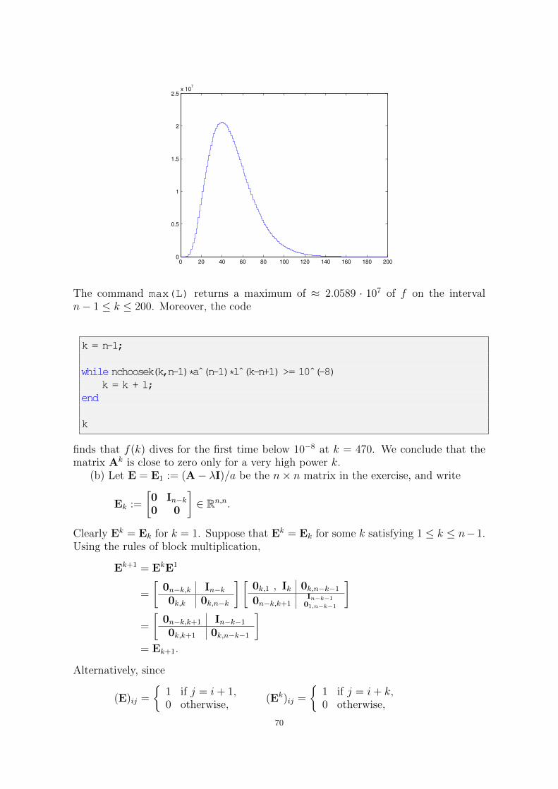
0 20 40 60 80 100 120 140 160 180 2000

0.5

1

1.5

2

2.5x 10

7

The command max(L) returns a maximum of ≈ 2.0589 · 107 of f on the intervaln− 1 ≤ k ≤ 200. Moreover, the code

k = n-1;

while nchoosek(k,n-1)*a (n-1)*l (k-n+1) >= 10 (-8)k = k + 1;

end

k

finds that f(k) dives for the first time below 10−8 at k = 470. We conclude that thematrix Ak is close to zero only for a very high power k.

(b) Let E = E1 := (A− λI)/a be the n× n matrix in the exercise, and write

Ek :=

[0 In−k0 0

]∈ Rn,n.

Clearly Ek = Ek for k = 1. Suppose that Ek = Ek for some k satisfying 1 ≤ k ≤ n−1.Using the rules of block multiplication,

Ek+1 = EkE1

=

[0n−k,k In−k0k,k 0k,n−k

] [0k,1 , Ik 0k,n−k−10n−k,k+1

In−k−101,n−k−1

]=

[0n−k,k+1 In−k−10k,k+1 0k,n−k−1

]= Ek+1.

Alternatively, since

(E)ij =

1 if j = i+ 1,0 otherwise,

(Ek)ij =

1 if j = i+ k,0 otherwise,

70

one has

(Ek+1)ij = (EkE)ij =∑`

(Ek)i`(E)`j = (Ek)i,i+k(E)i+k,j = 1 · (E)i+k,j

=

1 if j = i+ k + 1,0 otherwise,

By induction we conclude that Ek = Ek for any k satisfying 1 ≤ k ≤ n, with theconvention that En = En = 0n,n. We summarize that the matrix E is nilpotent ofdegree n.

(c) Since the matrices E and I commute, the binomial theorem and (b) yield

Ak = (aE + λI)k =

mink,n−1∑j=0

(k

j

)λk−jajEj.

Since (Ej)1,n = 0 for 1 ≤ j ≤ n− 2 and (En−1)1,n = 1, it follows that

(Ak)1,n =

mink,n−1∑j=0

(k

j

)λk−jaj(Ej)1,n =

(k

n− 1

)λk−n+1an−1 = f(k),


Exercise 11.31: A special norm

We show that ‖ · ‖t inherits the three properties that define a norm from the operatornorm ‖ · ‖1. For arbitrary matrices A,B and scalar a, we have

(1) Positivity. One has ‖B‖t = ‖DtU∗BUD−1t ‖1 ≥ 0, with equality holding

precisely when DtU∗BUD−1t is the zero matrix, which happens if and only if

B is the zero matrix.(2) Homogeneity. For any scalar a ∈ C,

‖aB‖t = ‖aDtU∗BUD−1t ‖1 = |a| · ‖DtU

∗BUD−1t ‖1 = |a| · ‖B‖t.(3) Subadditivity. One has

‖A + B‖t = ‖DtU∗(A + B)UD−1t ‖1

≤ ‖DtU∗AUD−1t ‖1 + ‖DtU

∗BUD−1t ‖1= ‖A‖t + ‖B‖t.

Since ‖ · ‖1 is an operator norm, it is consistent. For any matrices A,B for which theproduct AB is defined, therefore,

‖AB‖t = ‖DtU∗ABUD−1t ‖1

= ‖DtU∗AUD−1t DtU

∗BUD−1t ‖1≤ ‖DtU

∗AUD−1t ‖1‖DtU∗BUD−1t ‖1

= ‖A‖t‖B‖t,proving that ‖ · ‖t is consistent.

Exercise 11.33: When is A + E nonsingular?

Suppose ρ(A−1E) = ρ(A−1(−E)

)< 1. By part 2 of Theorem 11.32, I + A−1E is

nonsingular and therefore so is the product A(I + A−1E) = A + E.

71

CHAPTER 12

The Conjugate Gradient Method

Exercise 12.1: A-norm

Let A = LL∗ be a Cholesky factorization of A, i.e. L is lower triangular with positivediagonal elements. The A-norm then takes the form ‖x‖A =

√xTLL ∗ x = ‖L∗x‖.

Let us verify the three properties of a vector norm:

(1) Positivity: Clearly ‖x‖A = ‖L∗x‖ ≥ 0. Since L∗ in nonsingular, ‖x‖A =‖L∗x‖ = 0 if and only if L∗x = 0 if and only if x = 0.

(2) Homogeneity: ‖ax‖A = ‖L∗(ax)‖ = ‖aL∗x‖ = |a|‖L∗(x)‖ = |a|‖x‖A.(3) Subadditivity:

‖x + y‖A = ‖L∗(x + y)‖ = ‖L∗x + L∗y‖≤ ‖L∗x‖+ ‖L∗y‖ = ‖x‖A + ‖y‖A.

Exercise 12.2: Paraboloid

Given is a quadratic function Q(y) = 12yTAy − bTy, a decomposition A = UDUT

with UTU = I and D = diag(λ1, . . . , λn), new variables v = [v1, . . . , vn]T := UTy, anda vector c = [c1, . . . , cn]T := UTb. Then

Q(y) =1

2yTUDUTy − bTy =

1

2vTDv − cTv =

1

2

n∑j=1

λjv2j −

n∑j=1

cjvj,


Exercise 12.5: Steepest descent iteration

In the method of Steepest Descent we choose, at the kth iteration, the search directionpk = rk = b−Axk and optimal step length

αk :=rTk rk

rTkArk.

Given is a quadratic function

Q(x, y) =1

2

[x y

]A

[xy

]− bT

[xy

], A =

[2 −1−1 2

], b =

[00

],

and an initial guess x0 = [−1,−1/2]T of its minimum. The corresponding residual is

r0 = b−Ax0 =

[00

]−[

2 −1−1 2

] [−1−1/2

]=

[3/20

].

Performing the steps in Equation (12.7) twice yields

t0 = Ar0 =

[2 −1−1 2

] [3/20

]=

[3−3/2

], α0 =

rT0 r0rT0 t0

=9/4

9/2=

1

2,

72

x1 =

[−1−1/2

]+

1

2

[3/20

]=

[−1/4−1/2

], r1 =

[3/20

]− 1

2

[3−3/2

]=

[0

3/4

]

t1 = Ar1 =

[2 −1−1 2

] [0

3/4

]=

[−3/43/2

], α1 =

rT1 r1rT1 t1

=9/16

9/8=

1

2,

x2 =

[−1/4−1/2

]+

1

2

[0

3/4

]=

[−1/4−1/8

], r2 =

[0

3/4

]− 1

2

[−3/43/2

]=

[3/80

].

Moreover, assume that for some k ≥ 1 one has

(?) t2k−2 = 3 · 41−k[

1−1/2

], x2k−1 = −4−k

[12

], r2k−1 = 3 · 4−k

[01

],

(??) t2k−1 = 3 · 4−k[−12

], x2k = −4−k

[1

1/2

], r2k = 3 · 4−k

[1/20

].

Then

t2k = 3 · 4−k[

2 −1−1 2

] [1/20

]= 3 · 41−(k+1)

[1−1/2

],

α2k =rT2kr2krT2kt2k

=9 · 4−2k · (1

2)2

9 · 4−2k · 12

=1

2,

x2k+1 = −4−k[

11/2

]+

1

2· 3 · 4−k

[1/20

]= −4−(k+1)

[12

],

r2k+1 = 3 · 4−k[1/20

]− 1

2· 3 · 41−(k+1)

[1−1/2

]= 3 · 4−(k+1)

[01

],

t2k+1 = 3 · 4−(k+1)

[2 −1−1 2

] [01

]= 3 · 4−(k+1)

[−12

],

α2k+1 =rT2k+1r2k+1

rT2k+1t2k+1

=9 · 4−2(k+1)

9 · 4−2(k+1) · 2=

1

2,

x2k+2 = −4−(k+1)

[12

]+

1

2· 3 · 4−(k+1)

[01

]= −4−(k+1)

[1

1/2

],

r2k+2 = 3 · 4−(k+1)

[01

]− 1

2· 3 · 4−(k+1)

[−12

]= 3 · 4−(k+1)

[1/20

],

Using the method of induction, we conclude that (?), (??), and αk = 1/2 hold for anyk ≥ 1.

Exercise 12.8: Conjugate gradient iteration, II

Using x0 = 0, one finds

x1 = x0 +(b−Ax0)

T (b−Ax0)

(b−Ax0)TA(b−A2x0)(b−Ax0) =

bTb

bTAbb.

73

Exercise 12.9: Conjugate gradient iteration, III

By Exercise 12.8,

x1 =bTb

bTAbb =

9

18

[03

]=

[0

3/2

].

We find, in order,

p0 = r0 =

[03

], α0 =

1

2, r1 =

[320

],

β0 =1

4, p1 =

[3234

], α1 =

2

3, x2 =

[12

].

Since the residual vectors r0, r1, r2 must be orthogonal, it follows that r2 = 0 and x2

must be an exact solution. This can be verified directly by hand.

Exercise 12.10: The cg step length is optimal

For any fixed search direction pk, the step length αk is optimal if Q(xk+1) is as smallas possible, that is

Q(xk+1) = Q(xk + αkpk) = minα∈R

f(α),

where, by (12.4),

f(α) := Q(xk + αpk) = Q(xk)− αpTk rk +

1

2α2pT

kApk

is a quadratic polynomial in α. Since A is assumed to be positive definite, necessarilypTkApk > 0. Therefore f has a minimum, which it attains at

α =pTk rk

pTkApk

.

Applying (12.16) repeatedly, one finds that the search direction pk for the conjugategradient method satisfies

pk = rk +rTk rk

rTk−1rk−1pk−1 = rk +

rTk rkrTk−1rk−1

(rk−1 +

rTk−1rk−1

rTk−2rk−2pk−2

)= · · ·

As p0 = r0, the difference pk − rk is a linear combination of the vectors rk−1, . . . , r0,each of which is orthogonal to rk. It follows that pT

k rk = rTk rk and that the step lengthα is optimal for

α =rTk rk

pTkApk

= αk.

Exercise 12.11: Starting value in cg

As in the exercise, we consider the conjugate gradient method for Ay = r0, withr0 = b−Ax0. Starting with

y0 = 0, s0 = r0 −Ay0 = r0, q0 = s0 = r0,

one computes, for any k ≥ 0,

γk :=sTk sk

qTkAqk

, yk+1 = yk + γkqk, sk+1 = sk − γkAqk,

74

δk :=sTk+1sk+1

sTk sk, qk+1 = sk+1 + δkqk.

How are the iterates yk and xk related? As remarked above, s0 = r0 and q0 = r0 = p0.Suppose sk = rk and qk = pk for some k ≥ 0. Then

sk+1 = sk − γkAqk = rk −rTk rk

pTkApk

Apk = rk − αkApk = rk+1,

qk+1 = sk+1 + δkqk = rk+1 +rTk+1rk+1

rTk rkpk = pk+1.

It follows by induction that sk = rk and qk = pk for all k ≥ 0. In addition,

yk+1 − yk = γkqk =rTk rk

pTkApk

pk = xk+1 − xk, for any k ≥ 0,

so that yk = xk − x0.

Exercise 12.17: Program code for testing steepest descent

Replacing the steps in (12.17) by those in (12.7), Algorithm 12.14 changes into thefollowing algorithm for testing the method of Steepest Descent.

function [V,K] = sdtest(m, a, d, tol, itmax)R = ones(m)/(m+1) 2; rho = sum(sum(R.*R)); rho0 = rho;V = zeros(m,m);T1=sparse(toeplitz([d, a, zeros(1,m-2)]));for k=1:itmax

if sqrt(rho/rho0) <= tolK = k; return

endT = T1*R + R*T1;a = rho/sum(sum(R.*T)); V = V + a*R; R = R - a*T;rhos = rho; rho = sum(sum(R.*R));

endK = itmax + 1;

Listing 12.1. Testing the method of Steepest Descent

To check that this program is correct, we compare its output with that of cgtest.

[V1, K] = sdtest(50, -1, 2, 10 (-8), 1000000);[V2, K] = cgtest(50, -1, 2, 10 (-8), 1000000);surf(V2 - V1);

Running these commands yields Figure 1, which shows that the difference betweenboth tests is of the order of 10−9, well within the specified tolerance.

As in Tables 12.13 and 12.15, we let the tolerance be tol = 10−8 and run sdtestfor the m×m grid for various m, to find the number of iterations Ksd required before||rKsd

||2 ≤ tol · ||r0||2. Choosing a = 1/9 and d = 5/18 yields the averaging matrix, andwe find the following table.

n 2 500 10 000 40 000 1 000 000 4 000 000

Ksd 37 35 32 26 24

75

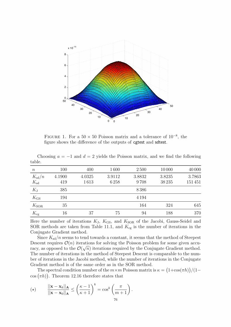
0

10

20

30

40

50

0

10

20

30

40

50

0

2

4

6

8

x 10−10

Figure 1. For a 50 × 50 Poisson matrix and a tolerance of 10−8, thefigure shows the difference of the outputs of cgtest and sdtest.

Choosing a = −1 and d = 2 yields the Poisson matrix, and we find the followingtable.

n 100 400 1 600 2 500 10 000 40 000

Ksd/n 4.1900 4.0325 3.9112 3.8832 3.8235 3.7863Ksd 419 1 613 6 258 9 708 38 235 151 451

KJ 385 8 386

KGS 194 4 194

KSOR 35 164 324 645

Kcg 16 37 75 94 188 370

Here the number of iterations KJ, KGS, and KSOR of the Jacobi, Gauss-Seidel andSOR methods are taken from Table 11.1, and Kcg is the number of iterations in theConjugate Gradient method.

Since Ksd/n seems to tend towards a constant, it seems that the method of SteepestDescent requires O(n) iterations for solving the Poisson problem for some given accu-racy, as opposed to the O(

√n) iterations required by the Conjugate Gradient method.

The number of iterations in the method of Steepest Descent is comparable to the num-ber of iterations in the Jacobi method, while the number of iterations in the ConjugateGradient method is of the same order as in the SOR method.

The spectral condition number of them×m Poisson matrix is κ =(1+cos(πh)

)/(1−

cos(πh)). Theorem 12.16 therefore states that

(?)||x− xk||A||x− x0||A

≤(κ− 1

κ+ 1

)k= cosk

(π

m+ 1

).

76

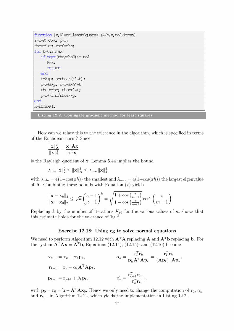
function [x,K]=cg_leastSquares (A,b,x,tol,itmax)r=b-A’*A*x; p=r;rho=r’*r; rho0=rho;for k=0:itmax

if sqrt(rho/rho0)<= tolK=k;return

endt=A*p; a=rho /(t’*t);x=x+a*p; r=r-a*A’*t;rhos=rho; rho=r’*r;p=r+(rho/rhos)*p;

endK=itmax+1;

Listing 12.2. Conjugate gradient method for least squares

How can we relate this to the tolerance in the algorithm, which is specified in termsof the Euclidean norm? Since

‖x‖2A‖x‖22

=xTAx

xTx

is the Rayleigh quotient of x, Lemma 5.44 implies the bound

λmin‖x‖22 ≤ ‖x‖2A ≤ λmax‖x‖22,

with λmin = 4(1−cos(πh)

)the smallest and λmax = 4

(1+cos(πh)

)the largest eigenvalue

of A. Combining these bounds with Equation (?) yields

‖x− xk‖2‖x− x0‖2

≤√κ

(κ− 1

κ+ 1

)k=

√1 + cos

(π

m+1

)1− cos

(π

m+1

) cosk(

π

m+ 1

).

Replacing k by the number of iterations Ksd for the various values of m shows thatthis estimate holds for the tolerance of 10−8.

Exercise 12.18: Using cg to solve normal equations

We need to perform Algorithm 12.12 with ATA replacing A and ATb replacing b. Forthe system ATAx = ATb, Equations (12.14), (12.15), and (12.16) become

xk+1 = xk + αkpk, αk =rTk rk

pTkATApk=

rTk rk(Apk)TApk

,

rk+1 = rk − αkATApk,

pk+1 = rk+1 + βkpk, βk =rTk+1rk+1

rTk rk,

with p0 = r0 = b−ATAx0. Hence we only need to change the computation of r0, αk,and rk+1 in Algorithm 12.12, which yields the implementation in Listing 12.2.

77

Exercise 12.23: Krylov space and cg iterations

(a) The Krylov spaces Wk are defined as

Wk := spanr0,Ar0, . . . ,A

k−1r0.

Taking A,b,x = 0, and r0 = b − Ax = b as in the Exercise, these vectors can beexpressed as

[r0,Ar0,A

2r0]

=[b,Ab,A2b

]=

400

, 8−40

, 20−16

4

.(b) As x0 = 0 we have p0 = r0 = b. We have for k = 0, 1, 2, . . . Equations (12.14),

(12.15), and (12.16),

xk+1 = xk + αkpk, αk =rTk rk

pTkApk,

rk+1 = rk − αkApk,

pk+1 = rk+1 + βkpk, βk =rTk+1rk+1

rTk rk,

which determine the approximations xk. For k = 0, 1, 2 these give

α0 =1

2, x1 =

200

, r1 =

020

, β0 =1

4, p1 =

120

,α1 =

2

3, x2 =

1

3

840

, r2 =1

3

004

, β1 =4

9, p2 =

1

9

4812

,α2 =

3

4, x3 =

321

, r3 =

000

, β2 = 0, p3 =

000

.(c) By definition we have W0 = 0. From the solution of part (a) we know

that Wk = span(b0,Ab0, . . . ,Ak−1b0), where the vectors b, Ab and A2b are linearly

independent. Hence we have dimWk = k for k = 0, 1, 2, 3.From (b) we know that the residual r(3) = b−Ax(3) = 0. Hence x(3) is the exact

solution to Ax = b.We observe that r0 = 4e1, r1 = 2e2 and r2 = (4/3)e3 and hence the rk for k = 0, 1, 2

are linear independent and orthogonal to each other. Thus we are only left to showthat Wk is the span of r0, . . . , rk−1. We observe that b = r0, Ab = 2r0 − 2r1 andA2b = 5r0 − 8r1 + 3r2. Hence span(b,Ab, . . . ,Abk−1) = span(r0, . . . , rk−1) for k =1, 2, 3. We conclude that, for k = 1, 2, 3, the vectors r0, . . . , rk−1 form an orthogonalbasis for Wk.

One can verify directly that p0,p1, and p2 are A-orthogonal. Moreover, observingthat b = p0, Ab = (5/2)p0 − 2p1, and A2b = 7p0 − (28/3)p1 + 3p2, it follows that

span(b,Ab, . . . ,Abk−1) = span(p0, . . . ,pk−1), for k = 1, 2, 3.

We conclude that, for k = 1, 2, 3, the vectors p0, . . . ,pk−1 form an A-orthogonal basisfor Wk.

78

By computing the Euclidean norms of r0, r1, r2, r3, we get∥∥r0∥∥2 = 4,∥∥r1∥∥2 = 2,

∥∥r2∥∥2 = 4/3,∥∥r3∥∥2 = 0.

It follows that the sequence (‖rk‖)k is monotonically decreasing. Similarly, one finds(∥∥xk − x∥∥2

)3k=0

=(√

10,√

6,√

14/9, 0),

which is clearly monotonically decreasing.

Exercise 12.26: Another explicit formula for the Chebyshev polynomial

It is well known, and easily verified, that cosh(x+y) = cosh(x) cosh(y)+sinh(x) sinh(y).Write Pn(t) = cosh

(n · arccosh(t)

)for any integer n ≥ 0. Writing φ = arccosh(t), and

using that cosh is even and sinh is odd, one finds

Pn+1(t) + Pn−1(t)

= cosh((n+ 1)φ

)+ cosh

((n− 1)φ

)= cosh(nφ) cosh(φ) + sinh(nφ) sinh(φ) + cosh(nφ) cosh(φ)− sinh(nφ) sinh(φ)

= 2 cosh(φ) cosh(nφ)

= 2tPn(t).

It follows that Pn(t) satisfies the same recurrence relation as Tn(t). Since in additionP0(t) = 1 = T0(t), necessarily Pn(t) = Tn(t) for any n ≥ 0.

Exercise 12.28: Maximum of a convex function

This is a special case of the maximum principle in convex analysis, which states thata convex function, defined on a compact convex set Ω, attains its maximum on theboundary of Ω.

Let f : [a, b]→ R be a convex function. Consider an arbitrary point x = (1−λ)a+λb ∈ [a, b], with 0 ≤ λ ≤ 1. Since f is convex,

f(x) = f((1− λ)a+ λb

)≤ (1− λ)f(a) + λf(b)

≤ (1− λ) maxf(a), f(b)+ λmaxf(a), f(b) = maxf(a), f(b).It follows that f(x) ≤ maxf(a), f(b) and that f attains its maximum on the bound-ary of its domain of definition.

79

CHAPTER 13

Numerical Eigenvalue Problems

Exercise 13.5: Nonsingularity using Gerschgorin

We compute the Gerschgorin disks

R1 = R4 = C1 = C4 = z ∈ C : |z − 4| ≤ 1,R2 = R3 = C2 = C3 = z ∈ C : |z − 4| ≤ 2.

Then, by Gerschgorin’s Circle Theorem, each eigenvalue of A lies in

(R1 ∪ · · · ∪R4) ∩ (C1 ∪ · · · ∪ C4) = z ∈ C : |z − 4| ≤ 2.In particular A has only nonzero eigenvalues, implying that A must be nonsingular.

Exercise 13.6: Gerschgorin, strictly diagonally dominant matrix

Suppose A is a strictly diagonally dominant matrix. For such a matrix, one findsGerschgorin disks

Ri =

z ∈ C : |z − aii| ≤

∑j 6=i

|aij|

.

Since |aii| >∑

j 6=i |aij| for all i, the origin is not an element of any of the Ri, and

therefore neither of the union⋃Ri, nor of the intersection (

⋃Ri) ∩ (

⋃Ci) (which is

smaller). Then, by Gerschgorin’s Circle Theorem, A only has nonzero eigenvalues,implying that det(A) = det(A− 0 · I) 6= 0 and A is nonsingular.

Exercise 13.8: Continuity of eigenvalues

For a given matrix A = (aij)ij ∈ Rn×n, write

A(t) := D + t(A−D), D := diag(a11, . . . , ann), t ∈ R,for the affine combinations of A and its diagonal part D. Let t1, t2 ∈ [0, 1], witht1 < t2, so that A(t1),A(t2) are convex combinations of A and D. For any eigenvalueµ of A(t2), we are asked to show that A(t1) has an eigenvalue λ such that

(?) |λ− µ| ≤ C(t2 − t1)1/n, C ≤ 2(‖D‖2 + ‖A−D‖2

).

In particular, every eigenvalue of A(t) is a continuous function of t.Applying Theorem 13.7 with A(t1) and E = A(t2) − A(t1), one finds that A(t1)

has an eigenvalue λ such that

|λ− µ| ≤(‖A(t1)‖2 + ‖A(t2)‖2

)1−1/n‖A(t2)−A(t1)‖1/n2 .

Applying the triangle inequality to the definition of A(t1) and A(t2), and using thatthe function x 7−→ x1−1/n is monotone increasing,

|λ− µ| ≤(

2‖D‖2 + (t1 + t2)‖A−D‖2)1−1/n

‖(A−D)‖1/n2 (t2 − t1)1/n.

80

Finally, using that t1 + t2 ≤ 2, that the function x 7−→ x1/n is monotone increasing,and that ‖(A−D)‖2 ≤ 2‖D‖2 + 2‖(A−D)‖2, one obtains (?).

Exercise 13.12: ∞-norm of a diagonal matrix

Let A = diag(λ1, . . . , λn) be a diagonal matrix. The spectral radius ρ(A) is the absolutevalue of the biggest eigenvalue, say λi, of A. One has

‖A‖∞ = max‖x‖∞=1

‖Ax‖∞ = max‖x‖∞=1

max|λ1x1|, . . . , |λnxn| ≤ ρ(A),

as λ1, . . . , λn ≤ λi = ρ(A) and since the components of any vector x satisfy x1, . . . , xn ≤‖x‖∞. Moreover, this bound is attained for the standard basis vector x = ei, since‖Aei‖∞ = λi = ρ(A).

Exercise 13.15: Number of arithmetic operations

An arithmetic operation is a floating point operation, so we need not bother withany integer operations, like the computation of k + 1 in the indices. As we are onlyinterested in the overall complexity, we count only terms that can contribute to this.

For the first line involving C, the multiplication v’*C involves (n − k)2 floatingpoint multiplications and about (n−k)2 floating point sums. Next, computing the outerproduct v*(v’*C) involves (n − k)2 floating point multiplications, and subtractingC - v*(v’*C) needs (n − k)2 substractions. This line therefore involves 4(n − k)2

arithmetic operations. Similarly we find 4n(n − k) arithmetic operations for the lineafter that.

These 4(n − k)2 + 4n(n − k) arithmetic operations need to be carried out for k =1, . . . , n− 2, meaning that the algorithm requires of the order

N :=n−2∑k=1

(4(n− k)2 + 4n(n− k)

)arithmetic operations. This sum can be computed by either using the formulae for∑n−2

k=1 k and∑n−2

k=1 k2, or using that the highest order term can be found by evaluating

an associated integral. One finds that the algorithm requires of the order

N ∼∫ n

0

(4(n− k)2 + 4n(n− k)

)dk =

10

3n3


Exercise 13.17: Number of arithmetic operations

The multiplication v’*C involves (n − k)2 floating point multiplications and about(n− k)2 floating point sums. Next, computing the outer product v*(v’*C) involves(n−k)2 floating point multiplications, and subtracting C - v*(v’*C) needs (n−k)2

substractions. In total we find 4(n−k)2 arithmetic operations, which have to be carriedout for k = 1, . . . , n− 2, meaning that the algorithm requires of the order

N :=n−2∑k=1

4(n− k)2

81

arithmetic operations. This sum can be computed by either using the formulae for∑n−2k=1 k and

∑n−2k=1 k

2, or using that the highest order term can be found by evaluatingan associated integral. One finds that the algorithm requires of the order

N ∼∫ n

0

4(n− k)2dk =4

3n3


Exercise 13.18: Tridiagonalize a symmetric matrix

From w = Ev, β = 12vTw and z = w − βv we get z = w − vβ = Ev − 1

2vvTEv and

zT = vTE− 12vTEvvT. Using this yields

G = (I− vvT)E(I− vvT) = E− vvTE− EvvT + vvTEvvT

= E− v(vTE− 1

2vTEvvT)− (Ev − 1

2vvTEv)vT

= E− vzT − zvT.

Exercise 13.22: Counting eigenvalues

Let

A =

4 1 0 01 4 1 00 1 4 10 0 1 4

, α = 4.5.

Applying the recursive procedure described in Corollary 13.21, we find the diagonalelements d1(α), d2(α), d3(α), d4(α) of the matrix D in the factorization A−αI = LDLT,

d1(α) = 4− 9/2 = −1/2,

d2(α) = 4− 9/2− 12/(−1/2) = +3/2,

d3(α) = 4− 9/2− 12/(+3/2) = −7/6,

d4(α) = 4− 9/2− 12/(−7/6) = +5/14.

As precisely two of these are negative, Corollary 13.21 implies that there are preciselytwo eigenvalues of A strictly smaller than α = 4.5. As

det(A− 4.5I) = det(LDLT) = d1(α)d2(α)d3(α)d4(α) 6= 0,

the matrix A does not have an eigenvalue equal to 4.5. We conclude that the remainingtwo eigenvalues must be bigger than 4.5.

82

Exercise 13.23: Overflow in LDLT factorization

Since An is tridiagonal and strictly diagonally dominant, it has a unique LU factoriza-tion by Theorem 1.10. From Equations (1.16), one can determine the correspondingLDL∗ factorization. For n = 1, 2, . . ., let dn,k, with k = 1, . . . , n, be the diagonalelements of the diagonal matrix Dn in a symmetric factorization of An.

(a) We proceed by induction. Let n ≥ 1 be any positive integer. For the firstdiagonal element, corresponding to k = 1, Equations (1.16) immediately yield 5 +√

24 < dn,1 = 10 ≤ 10. Next, assume that 5 +√

24 < dn,k ≤ 10 for some 1 ≤k < n. We show that this implies that 5 +

√24 < dn,k+1 ≤ 10. First observe that(

5 +√

24)2

= 25 + 10√

24 + 24 = 49 + 10√

24. From Equations (1.16) we know that

dn,k+1 = 10− 1/dn,k, which yields dn,k+1 < 10 since dn,k > 0. Moreover, 5 +√

24 < dn,kimplies

dn,k+1 = 10− 1

dn,k> 10− 1

5 +√

24=

50 + 10√

24− 1

5 +√

24= 5 +

√24.

Hence 5 +√

24 < dn,k+1 ≤ 10, and we conclude that 5 +√

24 < dn,k ≤ 10 for any n ≥ 1and 1 ≤ k ≤ n.

(b) We have A = LDLT with L triangular and with ones on the diagonal. As aconsequence,

det(A) = det(L) det(D) det(L) = det(D) =n∏i=1

di >(5 +√

24)n.

In Matlab an overflow is indicated by Matlab returning Inf as result. At my computerthis happens at n = 310.

Exercise 13.24: Simultaneous diagonalization

Let A,B,U,D, A, and D−1/2 be as in the Exercise.(a) Since D−

12 , like any diagonal matrix, and A are symmetric, one has

AT = D−12TUATUTD−

12T

= D−12 UAUTD−

12 = A

(b) Since A is symmetric, it admits an orthogonal diagonalization A = UTDU. Let

E := UTD−12 UT. Then E, as the product of three nonsingular matrices, is nonsingular.

Its inverse is given explicitly by F := UD12 U, since

FE = UD12 UUTD−

12 UT = UD

12 D−

12 UT = UUT = I

and similar EF = I. Hence E−1 = F and E is nonsingular. Moreover, from A = UTDUfollows that UAUT = D, which gives

ETAE = UD−12 UAUTD−

12 UT = UAUT = D.

Similarly B = UTDU implies UBUT = D, which yields

ETBE = UD−12 UBUTD−

12 UT = UD−

12 D

12 D

12 D−

12 UT = I.

We conclude that for a symmetric matrix A and symmetric positive definite matrix B,the congruence transformation X 7−→ ETXE simultaneously diagonalizes the matricesA and B, and even maps B to the identity matrix.

83

Exercise 13.25: Program code for one eigenvalue

(a) Let A = tridiag(c,d, c) and x be as in the Exercise. The following Matlab pro-gram counts the number of eigenvalues k of A strictly less than x.

function k=count(c,d,x)n = length(d);k = 0; u = d(1)-x;if u < 0

k = k+1;endfor i = 2:n

umin = abs(c(i-1))*eps;if abs(u) < umin

if u < 0u = -umin;

elseu = umin;

endendu = d(i)-x-c(i-1) 2/u;if u < 0

k = k+1;end

end

(b) Let A = tridiag(c,d, c) and m be as in the Exercise. The following Matlab pro-gram computes a small interval [a, b] around the mth eigenvalue λm of A and returnsthe point λ in the middle of this interval.

function lambda = findeigv(c,d,m)n = length(d);a = d(1)-abs(c(1)); b = d(1)+abs(c(1));for i = 2:n-1

a = min(a, d(i)-abs(c(i-1))-abs(c(i)));b = max(b, d(i)+abs(c(i-1))+abs(c(i)));

enda = min(a, d(n)-abs(c(n-1)));b = max(b, d(n)+abs(c(n-1)));h = b-a;while abs(b-a) > eps*h

c0 = (a+b)/2;k = count(c,d,c0);if k < m

a = c0;else

b = c0;end

endlambda = (a+b)/2;

84

(c) The following table shows a comparison between the values and errors obtainedby the different methods.

method value error

exact 0.02413912051848666 0findeigv 0.02413912051848621 4.44 · 10−16

Matlab eig 0.02413912051848647 1.84 · 10−16

Exercise 13.26: Determinant of upper Hessenberg matrix (TODO)

85

CHAPTER 14

The QR Algorithm

Exercise 14.4: Orthogonal vectors

In the Exercise it is implicitly assumed that u∗u 6= 0 and therefore u 6= 0. If u andAu− λu are orthogonal, then

0 = 〈u,Au− λu〉 = u∗(Au− λu) = u∗Au− λu∗u.

Dividing by u∗u yields

λ =u∗Au

u∗u.

86

numerical linear algebra a solution manual · numerical linear algebra a solution manual georg...

Documents