minimising whole life costs of mixing anoxic and anaerobic ...€¦ · batch process variants are...

6th European Waste Water Management Conference & Exhibition

www.ewwmconference.com

Organised by Aqua Enviro Technology Transfer

MINIMISING WHOLE LIFE COSTS OF MIXING ANOXIC AND ANAEROBIC TANKS

Höfken, M., Steidl, W., Huber, P. and Björndal, J.,

INVENT Umwelt- und Verfahrenstechnik AG, Germany

Email: [email protected]

Abstract

In the field of wastewater treatment, efficient mixers are needed to suspend solids and

homogenise in large mixing and equalization tanks, especially in anaerobic and anoxic tanks for

full nutrient removal in the activated sludge process. The layout and design of these mixing

systems must also take into account process and reactor design. Otherwise the plant will not

perform properly, and will not comply with the specification.

This paper describes the basic demands on a mixing system. It then details the layout and design

process for large anaerobic basins at large-scale wastewater treatment plants, from basic design

to lab scale testing, CFD simulation and large scale testing after the start-up of the plant.

Keywords

Mixing; Plug-flow reactor; Complete-mix reactor, Activated Sludge Process, Wastewater

treatment

Introduction

Water purification is one of the most important environmental tasks today. This includes the

physico-chemical treatment of natural water for the supply of drinking water and the biological

treatment of wastewater before it is discharged. The status of wastewater treatment varies

from country to country. Most of the industrialized countries have a very good coverage in

wastewater treatment plants with more than 90 % of the inhabitants connected; whereas less

developed countries continue to suffer from lack of sewage collection systems, water and

wastewater treatment plants. The quality of the wastewater treatment can be segmented into

the following types of treatment:

1. Primary Treatment: Mechanical treatment using screens and primary

sedimentation to separate solid matter.

2. Secondary Treatment: Includes the oxidation of biodegradable organics, usually

referred to as BOD1 and COD2 by means of additional

oxygen. The most commonly applied process is the so-

called activated sludge process.

3. Tertiary Treatment: Includes the biological reduction of BOD and COD plus full

nutrient removal. In this case nitrates and ammonia are

also removed by using anaerobic processes. In these

1 BOD: Biological Oxygen Demand 2 COD: Chemical Oxygen Demand

http://www.ewwmconference.com/

mailto:[email protected]




processes the wastewater needs to be mixed without the

addition of oxygen.

In the EU tertiary treatment for full nutrient removal is obligatory for all member states since

May 1991 (EEC, 1991). This is a standard which currently has not yet been reached in all

member states. Many plants still have to be built and many have to be upgraded – a situation

which is typical for the status of wastewater treatment in many countries in the world. This is

the reason why the activated sludge process including mixing and aeration has become a key

topic in wastewater treatment.

The activated sludge process stands for a large variety of continuous, space and time-oriented

periodic processes. As mentioned before, the activated sludge process is used for BOD-removal

and complete nitrogen removal. Well-known variants are the preliminary

nitrification/denitrification and the post-denitrification (Metcalf and Eddy, 1991). Well-known

batch process variants are the Sequencing Batch Activated Sludge Reactor (SBASR), the Cyclic

Activated Sludge System (CASS) and the Intermittent Cycle Extended Aeration System (ICEAS)

which are covered in detail in the literature: Irvine, 1971; Wilderer and Schroeder, 1986 or

Metcalf and Eddy, 1991. All these biological purification processes as well as the known

standard activated sludge process include two major operations: mixing and aeration. Without

mixing and aeration an effective reduction of BOD and nitrogen is impossible. Since

approximately 70% of the total energy consumption is used for these two processes (Höfken et

al., 1995) a proper choice and design of such systems is indispensable. Hence, only innovative

and energy-efficient equipment should be used.

The above reasons clarify the importance of discussing the role and impact of mixing and

aeration processes on the biological treatment process. The paper at hand focuses on mixing

and presents the basic design rules for the selection and layout of mixers for activated sludge

treatment plants. Using the example of the design of mixers for a large wastewater treatment

plant it is shown how an intelligent selection and design of mixers can help to improve the

reactor behavior and reduce the investment and operating costs of a plant.

About Mixing

General

A review of the mixing systems available on the market for wastewater treatment reveals an

impressive number of different products (Höfken, 1993). In order to somewhat classify the large

variety it is possible to refer to the definitions of the basic mixing tasks as they are used in the

fields of chemical and process engineering. A distinction is made in process engineering

between the following basic mixing tasks:

➢ Homogenization Compensation of differences in concentration or

temperature

➢ Suspension Stirring up and suspending of solid particles

➢ Dispersion Liquid/liquid Emulsions, polymerization





Liquid/gas Aeration, mass transfer

➢ Heat transfer Intensifying of the heat transmission (cooling, heating)

Table 1: Overview of mixing systems

Mixer type Schematic Mixing task(s) Applications

Horizontal

Propeller Mixers

(slow-speed)

Homogenization,

Suspension

biological phosphorus

removal, denitrification

Horizontal Propeller

Mixers

(high-speed)

Homogenization,

Suspension

(higher-viscosity fluids)

Storm water tanks,

sludge tanks

Blade mixer

Homogenization,

Suspension, Dispersion

Biological phosphorus

removal, denitrification

(Mainly in carousel

basins)

Hyperboloid mixers and

mixer/aerators

Homogenization,

Suspension, Dispersion,

Heat transfer

Biological phosphorus

removal, denitrification,

BOD-removal,

nitrification, intermittent

processes, sludge

treatment

Surface aerators

Suspension, Dispersion

BOD-Removal,

Nitrification

Self-aspirating

submerged aerators

Dispersion

BOD-Removal,

Nitrification, sludge

treatment

Self-aspirating helical

aerators

Dispersion

BOD-Removal,

Nitrification, sludge

treatment





Digested sludge

Mixers

Homogenization Sludge digesters

Note: The mixing tasks marked in bold type should preferably be performed using

the mixing system assigned to them in the above table. In more than a few

cases this may be inconsistent with normal applications in wastewater

treatment

This breakdown leads to a classification of all the different types of mixing systems available on

the market today that are used for wastewater treatment and enables an example of

application in wastewater treatment to be found without difficulty for each mixing task shown

in table 1.

Mixing is one of the most important unit processes used in the treatment of water and

wastewater. Figure 1 shows a typical flow diagram of a wastewater treatment plant and

illustrates in which treatment steps mixing is, or can be involved.

Figure 1: Mixing applications in wastewater treatment

The process starts in the mixing and equalization basin where mixers are used to homogenize

temperature and load peaks. Flash-mixing (fast and intense mixing) is needed in the

neutralization chamber. Precipitation and flocculation processes also strongly depend on the





correct design of the mixing equipment. During precipitation mixers shall mix the precipitant

fast and thoroughly with the wastewater whereas during flocculation the mixers shall supply

gentle mixing with low shear to allow for a good suspension and build-up of floc. In the

anaerobic or anoxic processes, mixers for “Biological Phosphorus Elimination” and

“Denitrification” have to supply a flow-field which ensure that no sedimentation occurs at the

bottom and which totally suspends and homogenises the sludge floc. Additional criteria are the

retention time and reactor type behavior of the tanks which is influenced severely by the choice

and the design of the mixers. This is one very important application for mixers which will be the

focussed on in this paper and discussed in more detail in the following chapters.

Mixing also plays a major role in the aerobic steps in which BOD is removed and nitrification is

achieved. Either aeration is realized using mixers which disperse the air in bubbles which then

transfer their oxygen into the water or membrane aerators are used to produce bubbles. In the

latter case the airflow itself has to provide sufficient mixing to avoid sedimentation of sludge

floc and to prevent short-circuiting. The important role of mixing in aerated tanks is highly

underestimated in many designs.

Furthermore mixing is needed in the treatment of waste sludge. This shows that in almost all

treatment steps mixing plays an important role and can decide about the quality of the overall

treatment result.

Fluid Mechanical Considerations

Basic Considerations

Denitrification and biological phosphorus elimination are anaerobic processes, i.e. oxygen-

transfer via the free surface is undesirable and negatively affects the biological processes. A

certain degree of turbulence promotes the work of bacteria since the floc remains limited in size

and is provided to a greater extent with substrate as a result of a larger surface area and the

occurrence of periodic stress conditions. The main requirement is to distribute the activated

sludge floc as evenly as possible and to avoid dead zones and short circuiting in the reactors.

These preliminary observations raise the question of the optimum flow conditions in the

activated sludge tank. In order to prevent the activated sludge floc from settling on the bottom

of the tank, it makes sense to produce the maximum possible flow rates together with a certain

degree of turbulence near to the bottom. If we look at the macro-scale flow pattern it is

sufficient here to circulate the tank volume uniformly in order to achieve the most even

distribution; too much turbulence in this case would have a negative effect on efficiency. It is

especially important to avoid surface turbulence, since this would increase oxygen-transfer

capacity via the free surface.

If we look at the micro-scale flow pattern, higher turbulent fluctuations which can whirl up

sedimentations are desirable at the bottom of the tank.





Since the majority of sewage treatment plants are built with rectangular tanks, the flow in this

type of tank will be examined here in more detail. The design of mixing systems in carousel and

circular tanks is described in Höfken, 1993. The design rules are similar to the ones presented

below.

It has been deduced that the most favorable energy conditions are obtained for suspension

using tank bottom mixing systems arranged centrally in the tank. Clarification is needed on the

question of the minimum flow velocity required at the bottom of the tank.

Analytical Approach

In order to arrive at a practical method for calculating the minimum bottom velocities in a

reactor it is necessary to initially define the critical point for deposits in the reactor under

question. It is shown that the critical area is normally close to the edge of the tank at the point

where the horizontal flow is changing to the vertical direction. Here the bottom boundary layer

reaches its full length and has normally increased to such an extent that a greater number of

particles can penetrate the viscous sub-layer due to the zones of lower flow rates present close

to the bottom (wall). It is known from experience that the corner flow itself is not a critical area

with respect to flow patterns produced by radial mixing systems near to the bottom because an

eddy flow with a strong upward component occurs as a result of slowing down the rotation

flow, preventing the formation of deposits at this point. The flow patterns shown in Figure 2 are

obtained from an examination of the change of direction of the flow at the wall and on the right

hand side a single particle in the bottom boundary layer is shown schematically.

Figure 2: Change of direction of flow near the wall and a single particle in the bottom

boundary layer

The critical point can be defined in two ways: by selecting a point on the bottom or on the wall

outside the area of influence of the corner. Own investigations (Höfken, 1994) have shown that

the axial speeds near the wall directly after the change of direction are even slightly higher than

the maximum measured radial bottom velocities. The influence of the corner flow can be

eliminated by selecting a distance of a=L/10 from the wall and a distance b=L/30 from the

bottom for both critical points. There is no danger of deposits forming in the corner vortex as

higher velocities and turbulences occur here, which prevent particle deposits provided the

minimum velocity calculated below is observed. The possibility exists here, however, to reduce





to a minimum the losses that occur as a result of vortex formation by furnishing the corners with

concrete haunches. Both definitions of the reference point can be used to the same equivalent

extent. For the initial theoretical calculation of the minimum bottom velocity given below,

however, it is simpler to select a point on the bottom at a distance of L/10 because boundary

layer observations are easier here.

Two limit cases can be formulated to estimate the forces exerted by the fluid on the particles

contained in the boundary layer at the bottom:

1. Only the wall shear stress acts on the particles

2. A tractive force is active with velocity v as a result of the flow.

According to Latzel (1986), limit case 2 leads to a condition for the limit case of the minimum

suspension of a single particle (P0). Since this case is not of any technical relevance, it is not

considered here. We shall consider case 1, the effect of the wall shear stress. The behavior of

the turbulent velocity profile near the wall can be derived from the Prandtl-mixing length, which

can be stated in general as follows based on Levich (1962):

30,

305,

5,

ln5,25,5

2,1)1,0(arctan10)(

yzoneturbulent

yzonetransition

ysublayerviscous

y

y

y

u

yu

(1)

where u is the so-called wall shear stress velocity and y+ is the dimensionless wall distance. The

following definitions apply:

;

wu

(2)

uy

y

(3)

In the case of an even or slightly arched bottom, the following formula applies for the local wall

shear stress according to Schlichting (1965):

2'

2

uc L

fW

(4)

For boundary layers that are turbulent from the start the following formula can be obtained by

recalculation in contrast to the proposal by Latzel (1986):





5

1' Re0592,0

lfc

(5)

This then leads to an implicit calculation method for uoo. Equation (5) is used for further

calculation. The Reynolds number is formed here with development length l of the boundary

layer. Length l is dependent on the mixer design and on the tank size.

ul

lRe

(6)

If (3), (4) and (5) are used in (2), an equation is obtained after conversion for determining the

flow velocity at the critical point, which corresponds to the minimum bottom velocity.

910

1,0

1,0

184,0

luu

(7)

In order to calculate this explicitly, an equilibrium of forces must now be created between the

shear stress forces and the gravity forces acting on the particles.

g

dd Pw

P

64

32

(8)

Use of (2) in (8) results after conversion in an equation between the dimensionless units Re and

Ar:

L

PP gdud

2

32

3

2

(9)

Ar

3

2Re2

(10)

By calculating the Archimedes' number it is possible to calculate u and use it in (7) as the

missing variable. Various equations can be applied for length l of the boundary layer depending

on the mixing system and the method used to create the flow. Figure 3 shows the minimum

bottom velocity for various particle diameters as a function of length l=f (tank size, method used

to create the flow).





Developing Length of Boundary Layer [m]

Minimum Bottom Velocity [m/s]

0 1 2 3 4 5 6 7 8 9 10

0

0,05

0,1

0,15

0,2

Mindestsohlgeschwindigkeit

(c)LSTM,mh”

d=60E-6 m

d=100E-6 m

d=200E-6 m

Figure 3: Minimum bottom velocity as a function of tank size

It can be seen that bottom flow velocities of 15 cm/s are certainly adequate enough to stir up

activated sludge and keep it suspended. The recommended design particle size is dp=100 m

(middle curve), the real value for samples from a great number of wastewater treatment plants

was dp = 60 m as depicted in the bottom curve. Bottom velocities of 10 cm/s therefore should

also be sufficient, however without any safety against variations. This statement does not

contradict the recommendation of the ATV3 to maintain bottom velocities of 10 – 30 cm/s, but

clearly shows that a demand for minimum bottom velocities greater than 30 cm/s is

unjustifiable. Even maximum particle sizes do not demand bottom velocities greater than

20cm/s. It is fully adequate, therefore, even taking possible density fluctuations into account, to

apply bottom velocities greater than 15 cm/s.

The above considerations also show that it is unrealistic to specify particular power inputs, since

these cannot guarantee particular bottom velocities. The power input required is dependent on

the mixing system and on the type of flow generation as described above. To try to ensure

adequate bottom velocities by specifying minimum power inputs is only possible if very high and

unnecessary safety factors are accepted. Just how drastically the demand for excessive bottom

velocities affects the overall power consumption and thus the operating costs of a plant is

described below.

3ATV: German Association for Water and Pollution Control





The following equation can be used to describe the relationship between the bottom velocity at

the critical point and the rotational speed of the mixing element

Rd

uCn

(11)

where constant C is dependent on the type of flow generation and on the mixing system. At this

point it is important to note that the minimum bottom velocity consists of the average velocity

and the turbulent fluctuations according to

'

uuu

(12)

If the turbulent fluctuations are neglected at the design stage, safety is assured but the power

consumption will increase. The following equation applies to the power:

53

RL dnNeP

(13)

where Ne is the power or Newton number (a variable dependent on the mixing element, see

table 2). Table 2 shows Newton numbers for various mixers for the Reynolds number range

Re>104.

Table 2: Newton numbers of standard mixers

Mixing System Newton Number, Re > 104

Propeller mixer, 3-blade, o25 0,35

Blade mixer, 6-blade 5,00

Hyperboloid mixer, 8 transport ribs 0,25

Hyperboloid mixer, 8 transport ribs

and shear ribs for aeration

0,50

Use of (11) in (13) taking (12) into consideration results in

2

3'

RL duu

NeP

(14)

The rotational speed and thus the bottom velocity are cubed in the power equation (i.e. even

small increases in specified bottom velocity cause the power consumption to increase at very

high rates). Equation (14) also shows that it is more favorable to choose slow-speed mixing

systems with large diameters than small fast-running systems. A further advantage concerns the

smaller shear stress acting on the bacteria floc, but this point will not be discussed here.





If the speed range and the turbulent fluctuation speed of a mixing system as well as constant C

are known, it is thus possible to implement a complete design for the mixing system for

activated sludge tanks. The exact procedure is described in Höfken, 1994. One way to determine

the constant C is to do measurements in model and in large scale. The second possibility is to

use numerical simulations like shown in the next paragraph. Ideal is the combined application of

both methods. In this case the experimental work is used to validate the numerical simulations.

The numerical simulations ensure the exact scale-up.

Example I

Error! Reference source not found. shows the velocity field of a hyperboloid mixer in a 400mm

x 400mm lab-scale tank. The measurements were executed using ultrasound-Doppler-

anemometry. Similar results can be obtained with laser-Doppler-anemometers. Such diagrams

can be used to determine the mixer speed needed to create a given velocity at a given point in

the basin. The velocity vectors show the magnitude of the velocity and the direction of the flow.

In the turbulent regime they are directly proportional to the tip speed of the mixer and can

therefore be used for design purposes.

Figure 4: Velocity field of a hyperboloid mixer close to the bottom of a squared tank

It is important to validate scale-ups which are based on experiments in model-scale. Figure 5

shows a comparison of the results obtained in the model-tank with results from a real

wastewater treatment plant in the Eiger-Northface region in Switzerland, which was equipped

with geometrically similar hyperboloid-mixers.





g

Figure 5: Measured bottom velocities in model and in large-scale

The comparison shows excellent agreement between model and large scale. More than 5 years

trouble-free operating experience of 24 HYPERCLASSIC-mixers support the exact design and

layout of these mixers.





Process Considerations

The two reactor types most commonly used in the biological treatment of wastewater are the

plug-flow reactor and the continuous-flow stirred-tank reactor or complete-mix reactor.

Figure 6: Plug-flow reactor

In a plug-flow reactor the fluid particles pass through the tank and are discharged in the same

sequence in which they enter. The particles retain their identity and remain in the tank for a

time equal to the theoretical detention time. This type of flow is approximated in long tanks

with a high length-to-width ratio in which longitudinal dispersion is minimal or absent.

Figure 7: Continuous-flow stirred-tank reactor

Complete mixing occurs when the particles entering the tank are dispersed immediately

throughout the tank. The particles leave the tank in proportion to their statistical population.

Complete mixing can be accomplished in round or square tanks if the contents of the tank are

uniformly and continuously distributed.

Figure 8: Continuous-flow stirred-tank reactor in series

A series of complete-mix reactors is used to model the flow regime that exists between the

hydraulic flow patterns corresponding to the complete-mix and plug-flow reactors. If the series

is composed of one reactor, the complete-mix regime prevails. If the series consists of an infinite

number of reactors in series the plug-flow regime prevails.

The choice of the reactor type is one very important design step which depends on several

operational factors such as: reaction kinetics, oxygen-transfer requirements, nature of the

wastewater, local conditions etc.. This means that the activated sludge tanks, which are

biological reactors were at one stage of the design process consciously or at least implicitly

designed as a plug-flow or a complete-mix reactor or a combination of both. This has to be

taken into account when the mixing equipment for the reactors is chosen, otherwise the

selection and design of the mechanical equipment may jeopardize the reactor design.





Case study I The following case study shows an example of a large wastewater treatment plant with 6

parallel trains which each consist of again 2 parallel lines of anaerobic, anoxic and oxic tanks.

The anoxic zones were designed as so-called cascaded denitrification tanks which consist of a

series of complete-mix reactors. In an extensive engineering study which included experimental

and numerical fluid mechanics (CFD4) the optimal type and number of mixers were selected.

One very important additional task was to clarify whether the series of complete-mix reactors

could be realized without building walls between the mixers as was initially planned.

Figure 9 shows three of the six trains with the chosen arrangement of the mixing equipment.

Each basin is 110m long, 8m wide and 4.1m deep (water depth). As the optimum mixing system

8 HYPERCLASSIC-Mixers were chosen for each basin of which the last 2 units were supplied as

mixer and aeration systems to allow for additional oxygen supply during the cold season. This

so-called bivalent zone was separated by a physical separating wall to avoid back-mixing of

oxygen-rich wastewater into the denitrification zone. In the left part of the drawing the

anaerobic zones in which biological phosphorus removal takes place are shown.

Figure 9: 60 of in total 96 HYPERCLASSIC-Mixers in a large wastewater treatment

plant

4 CFD: Computational Fluid Mechanics





The following graphs show results of the 3-dimensional computer simulation which had been

executed in the design phase to find the optimum design and to prove the reactor behavior. The

simulation concerned the flow created by the rotation of the mixers as well as the inflow of

wastewater and recirculation-flow. More than 2 million grid points were used to model the tank

and the mixers. The rotation of the mixers was modeled by using the so-called sliding grid

technique.

Figure 10 shows one whole tank in a cut through the symmetry plane. The color contour-plot

visualizes the magnitude of the velocities in z-direction (upwards/downwards-flow). By this

measure the velocity distribution between the mixers can be illustrated very nicely. It can be

clearly shown that there is a strong upwards flow between each pair of mixers which clearly

indicates the division of the long tank into single cells. If one compares the flow-pattern at the

overflow of the real separating wall and at the side wall to the flow between each pair of mixers,

this impression becomes even stronger. This unique flow pattern is called the production of

virtual walls between two mixers which can only be achieved with hyperboloid mixers. This was

one reason why HYPERCLASSIC-mixers were chosen for this project.

Figure 10: Numerical simulation of an activated sludge tank with 6 + 2 HYPERCLASSIC

Mixers comparing virtual and real separation walls






Mixers showing detail of virtual separation wall between one pair of mixers

Figure 11 shows the virtual wall between one pair of hyperboloid mixers in more detail. To

clearly show the similarity between the overflow at the real wall and the flow-pattern at a

virtual wall in

Figure 11 and

Figure 12 the color-contour plots are shown together with the corresponding velocity vectors.

These graphs illustrate the typical flow pattern caused by hyperboloid-mixers with the radial

flow originating from the mixer body over the bottom, going up the wall and returning to the

center of the mixed cell. Both graphs, for the real wall simulation and for the virtual wall

simulation look identical. This proves that hyperboloid mixers can create a series of complete-

mix reactors without building separating walls. This effect cannot be achieved with any other

type of mixer and is very beneficial to the plant design. Real separating walls normally cause

high overflow velocities which are undesirable because they increase the probability of short-

circuits on the downstream side of the wall. Real separating walls also contribute to higher total

hydraulic losses of the plant.






Mixers showing detail of real separation wall between one pair of mixers


Mixers showing detail of virtual separation wall between one pair of mixers





It is very important is to also know whether the detention time reaches the theoretical

detention time and whether short circuits occur in such a tank. To examine this a particle tracing

study was done to derive the detention time distributions. In total more than 20,000 particles

were added to the inflow of the tank and traced until they left the tank through the outlet.

Figure 14 shows 25 trajectories which enter the basin from the left side. The color of the

trajectories indicate the detention time. Figure 15 shows one single particle on its way through

the tank. It very nicely shows how the virtual and the real separation walls retain the particle

and increase the detention time.


Mixers showing detail of 25 trajectories of particles following the flow






Mixers showing detail of one trajectory following the flow

The statistical analysis of all particle trajectories finally results in the overall detention time

behavior of the reactor which in this case is very close to the theoretically expected value. This

shows how the proper design of a reactor and the selection of mixers can be achieved using

modern fluid mechanical engineering tools. Additionally tremendous investments in civil works

could be saved because no separating walls had to be built.






Mixers - Detention time distribution


Mixers – Picture of real plant with a total of 96 mixers





Mechanical

The mechanical design of mixers mainly concerns

1. Mechanical forces on the mixer element, e.g. propeller blades

2. Mechanical forces on the shaft

3. Mechanical forces on the drive, mainly gear-reducer and bearings

4. Mechanical forces on the bridge or support for the mixer

The mechanical forces on the mixer-element or the blades are caused by the flow-field around

the mixer-element. The resulting force normally can be split in a normal-component Fn and a

tangential-component Fz. These two components are relevant for the structural design of the

mixer-element. Since this design is mixer-dependent we will not further discuss it at this point.

For the shaft design it is more common to split the resulting main force into an axial-component

FAX and a circumferential component FU. The sum of all circumferential forces - the number is

dependent on the number of single blades or vanes of the mixer-element – times the valid

radius results in the total torque acting on shaft and gear-drive. Unfortunately the single forces

acting on each blade or vane do not act regularly on the blades but are, due to the turbulent

flow stochastically acting on the blades. This is the reason why for all kind of mixer-elements a

resulting radial force FR occurs. FR is a very important force for the design of the shaft and the

gear-drive. FR is the bigger the stronger the turbulent trailing vortices behind the blades are and

it decreases with the number of blades or vanes. This means that a two-blade propeller mixer

has a much higher resulting radial force than a four-bladed propeller mixer or a hyperboloid-

mixer with 8 transport-vanes.

Figure 18 shows the resulting axial and radial forces on a standard propeller-mixer. The induced

flow-field results in an upwards directed axial force and in a high radial force which tends to

bend the shaft. This means high mechanical loads on the shaft, the gear-drive and the bridge.

These type of mixers demand for very heavy design of shafts, gear-drives and bridges.





Figure 18: Axial and radial forces acting on a standard propeller-mixer

In comparison to the standard case Figure 19 shows the resulting axial and radial forces on a

hyperboloid-mixer. In this case only downward directed forces act on the shaft which cannot

bend the shaft and almost no radial forces occur due to the closed mixer-body with a high

number of single vanes. This is a significant advantage since the forces acting on the shaft, gear-

drive and bridge are much lower and - even more important – they are directed in the harmless

direction. Therefore the design for the shafts, gear-drives and bridges can be much lighter for

hyperboloid-mixers.

Figure 19: Axial and radial forces acting on a hyperboloid-mixer

L

Fax 2Fax 1

Fr

Vz

V

F ax

F r

L





Conclusions To achieve optimum purification power in wastewater treatment plants, advanced and efficient

mixing and aeration systems have to be used because mixing and aeration are the major

processes needed in the biological treatment of wastewater. Approximately 70% of the total

energy demand of a wastewater treatment plants is needed for these processes (Höfken et al.,

1995).

A study of systems available on the market showed that numerous systems are offered which

can be classified and compared using some simple considerations. It was shown that efficient

mixing systems should be bottom mounted and fluid mechanically optimized. Minimum bottom

velocities of approx. 15 to 20 cm/s are sufficient in most of the applications.

The design of mixing systems also influences the overall reactor behavior of the wastewater

treatment plant. Therefore it is crucial to select the mixing system in compliance with the initial

process design.

For the mechanical design of mixers it is important to understand the main forces acting on a

mixing system and the bridges. There are severe differences between standard propeller mixers

and modern hyperboloid mixers since the resulting axial forces on the mixing system are

significantly less harmful in the case of hyperboloid mixers. This results in a lighter design and

longer lifetime.

Acknowledgements We would like to thank the Berlin Water Authorities, who awarded us with the contract for the

engineering studies and the supply of 96 HYPERCLASSIC-Mixers plus bridges, for the

professional support and the excellent cooperation.

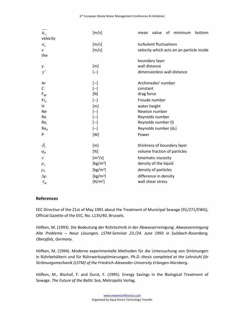
Symbols

a [m] distance from the wall b [m] distance from the bottom cw [--] friction number (particle)

dP [m] particle diameter

dR [m] diameter of mixer

g [m/s2] ground acceleration l [m] developing length of boundary layer n [Hz] number of revolutions u [m/s] velocity u(y+) [m/s] velocity in boundary layer uTip [m/s] tip-speed of mixer

u [--] wall shear stress velocity

u [m/s] minimum bottom velocity





u [m/s] mean value of minimum bottom

velocity

u

' [m/s] turbulent fluctuations

v [m/s] velocity which acts on an particle inside the boundary layer y [m] wall distance

y [--] dimensionless wall distance

Ar [--] Archimedes' number C [--] constant FW [N] drag force

FrP [--] Froude number

H [m] water height Ne [--] Newton number Re [--] Reynolds number Rel [--] Reynolds number (l)

ReP [--] Reynolds number (dP)

P [W] Power l [m] thickness of boundary layer

P [%] volume fraction of particles

[m2/s] kinematic viscosity

L [kg/m3] density of the liquid

P [kg/m3] density of particles

[kg/m3] difference in density W [N/m2] wall shear stress

References EEC Directive of the 21st of May 1991 about the Treatment of Municipal Sewage (91/271/EWG),

Official Gazette of the EEC, No. L135/40, Brussels.

Höfken, M. (1993). Die Bedeutung der Rührtechnik in der Abwasserreinigung. Abwassereinigung

Alte Probleme – Neue Lösungen, LSTM-Seminar 23./24. June 1993 in Sulzbach-Rosenberg,

Oberpfalz, Germany.

Höfken, M. (1994). Moderne experimentelle Methoden für die Untersuchung von Strömungen

in Rührbehältern und für Rührwerksoptimierungen. Ph.D.-thesis completed at the Lehrstuhl für

Strömungsmechanik (LSTM) of the Friedrich-Alexander-University Erlangen-Nürnberg.

Höfken, M., Bischof, F. and Durst, F. (1995). Energy Savings in the Biological Treatment of

Sewage. The Future of the Baltic Sea, Metropolis Verlag.





Irvine, R. L. and Davis, W.B. (1971). Proc. 26th. Ann. Ind. Waste Conf., Purdue Univ., Ann Arbor

Sc., Michigan.

Latzel, W. (1986). Mindestrührerdrehzahlen zum Suspendieren von Feststoffpartikeln. Ph.D.-

thesis completed at the Institute for Mechanical Process-Technology of the Friedrich-Alexander-

University Erlangen-Nürnberg.

Levich, V. G. (1962). Physicochemical Hydrodynamics. Prentice-Hall International, Inc., United

Kingdom and Eire.

Metcalf and Eddy (1991). Wastewater Engineering - Treatment, Disposal and Reuse. McGraw Hill

Inc.

Schlichting, H. (1965). Grenzschichttheorie. 5. erw. Aufl., G. Braun Verlag, Karlsruhe.

Updating of Statistical Data about Sewage Treatment in the EEC", SMBC/EEC, Final Report 2/90.

_____________________

HYPERCLASSIC is a registered trademark of INVENT Umwelt- und Verfahrenstechnik AG


minimising whole life costs of mixing anoxic and anaerobic ...€¦ · batch process variants are...

Documents