MiniCon Reformulation& Adaptive Re-Optimization

Zachary G. IvesUniversity of Pennsylvania

CIS 650 – Database & Information Systems

February 23, 2005

2

Administrivia

Next reading assignment: Urhan & Franklin – Query Scrambling Ives et al. – Adaptive Data Partitioning Compare the different approaches

One-page proposal of your project scope, goals, and means of assessing success/failure due next Monday, Feb. 28th

3

Today’s Trivia Question

4

Buckets, Rev. 2: The MiniCon Algorithm

A “much smarter” bucket algorithm: In many cases, we don’t need to perform the

cross-product of all items in all buckets Eliminates the need for the containment check

This – and the Chase & Backchase strategy of Tannen et al – are the two methods most used in virtual data integration today

5

Minicon Descriptions (MCDs)

Basically, a modification to the bucket approach “head homomorphism” – defines what variables

must be equated Variable-substituted version of the subgoals Mapping of variable names Info about what’s covered

Property 1: If a variable occurs in the head of a query, then

there must be a corresponding variable in the head of the MCD view

If a variable participates in a join predicate in the query, then it must be in the head of the view

6

MCD Construction

For each subgoal of the queryFor each subgoal of each view

Choose the least restrictive head homomorphism to match the subgoal of the query

If we can find a way of mapping the variables, then add MCD for each possible “maximal” extension of the mapping that satisfies Property 1

7

MCDs for Our Example5star(i) show(i, t, y, g), rating(i, 5, s)TVguide(t,y,g,r) show(i, t, y, g), rating(i, r, “TVGuide”)movieInfo(i,t,y,g) show(i, t, y, g)critics(i,r,s) rating(i, r, s)goodMovies(t,y) show(i, t, 1997, “drama”), rating(i, 5,

s)good98(t,y) show(i, t, 1998, “drama”), rating(i, 5, s)

view h.h. mapping goals sat.

5star(i) ii ii 2

TVguide(t,y,g,r)

tt, yy, gg tt, yy, gg, rr

1,2

movieInfo(i,t,y,g)

ii, tt, yy, gg

ii, tt, yy, gg

1

critics(i,r,s) ii, rr, ss ii, rr, ss 2

goodMovies(t,y)

tt,yy tt, yy 1,2

good98(t,y) tt,yy tt, yy 1,2

q(t) :- show(i, t, y, g), rating(i, r, s), r = 5

8

Combining MCDs

Now look for ways of combining pairwise disjoint subsets of the goals Greatly reduces the number of candidates! Also proven to be correct without the use of a

containment check

Variations need to be made for: Constants in general (I sneaked those in) “Semi-interval” predicates (x <= c)

Note that full-blown inequality predicates are co-NP-hard in the size of the data, so they don’t work

9

MiniCon Performance, Many Rewritings

Chain queries with 5 subgoals and all variables distinguished

0

2

4

6

8

10

1 2 3 4 5 6 7 8 9 10 11

Number of Views

Tim

e (

se

c)

MiniCon

Inverse

Bucket

10

Larger Query, Fewer Rewritings

Chain queries; 2 variables distinguished, query of length 12, views of lengths 2, 3, and 4

0

0.5

1

1.5

2

0 50 100 150

Number of Views

Tim

e (

se

c)

Minicon

Inverse

11

MiniCon and LAV Summary

The state-of-the-art for AQUV in the relational world of data integration It’s been extended to support “conjunctive XQuery” as well

Scales to large numbers of views, which we need in LAV data integration

A similar approach: Chase & Backchase by Tannen et al. Slightly more general in some ways – but:

Produces equivalent rewritings, not maximally contained ones Not always polynomial in the size of the data

12

Motivations for Adaptive Query Processing

Many domains where cost-based query optimization fails:

Complex queries in traditional databases: estimation error grows exponentially with # joins [IC91]

Querying over the Internet: unpredictable access rates, delays

Querying external data sources: limited information available about properties of this source

Monitor real-world conditions, adapt processing strategy in response

13

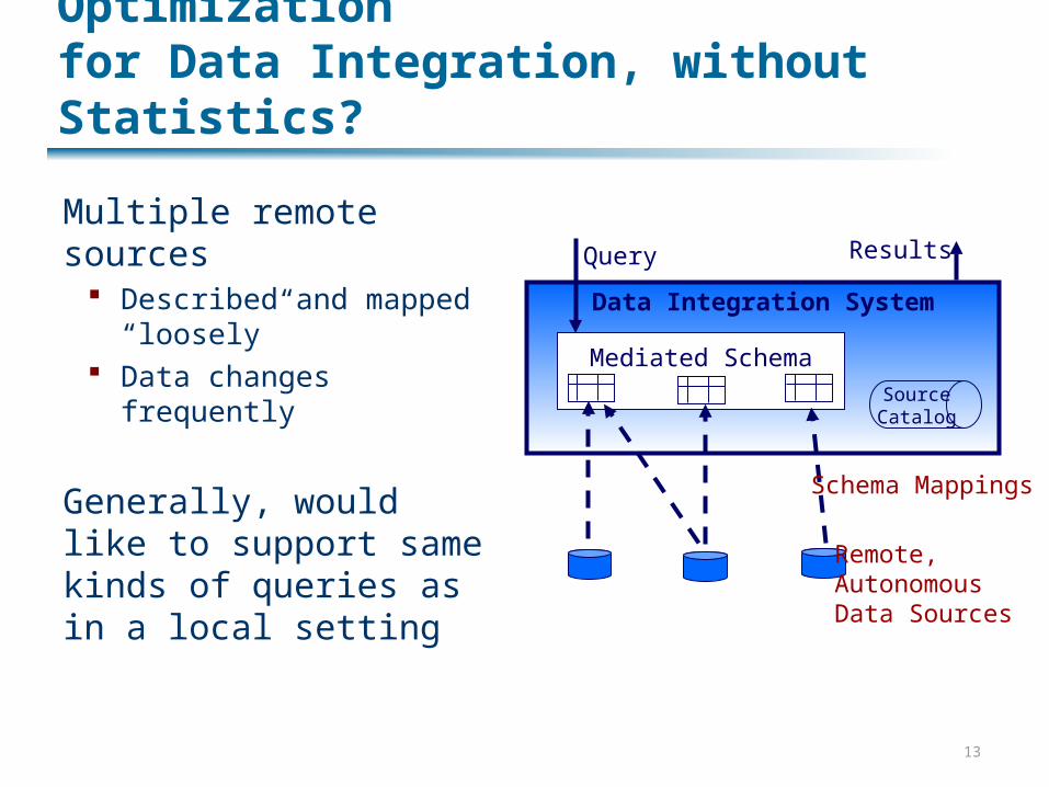
Can We Get RDBMS-Level Optimizationfor Data Integration, without Statistics?

Multiple remote sources Described and mapped

“loosely” Data changes frequently

Generally, would like to support same kinds of queries as in a local setting

Data Integration System

Mediated Schema

Remote,AutonomousData Sources

Schema Mappings

SourceCatalog

Query Results

14

What Are the Sources of Inefficiency?

Delays – we “stall” in waiting for I/O We’ll talk about this on Monday

Bad estimation of intermediate result sizes The focus of the Kabra and DeWitt paper

No info about source cardinalities The focus of the eddies paper – and Monday’s paper

The latter two are closely related Major challenges:

Trading off information acquisition (exploration) vs. use (exploitation)

Extrapolating performance based on what you’ve seen so far

15

Kabra and DeWitt

Goal: “minimal update” to a traditional optimizer in order to compensate for bad decisions

General approach: Break the query plan into stages Instrument it Allow for re-invocation of optimizer if it’s going

awry

16

Elements of Mid-Query Re-Optimization

Annotated Query Execution Plans Annotate plan with estimates of size

Runtime Collection of Statistics Statistics collectors embedded in execution

tree Keep overhead down

Dynamic Resource Re-allocation Reallocate memory to individual operations

Query Plan Modification May wish to re-optimize the remainder of query

17

Annotated Query Plans

We save at each point in the tree the expected: Sizes and cardinalities Selectivities of predicates Estimates of number of groups to be

aggregated

18

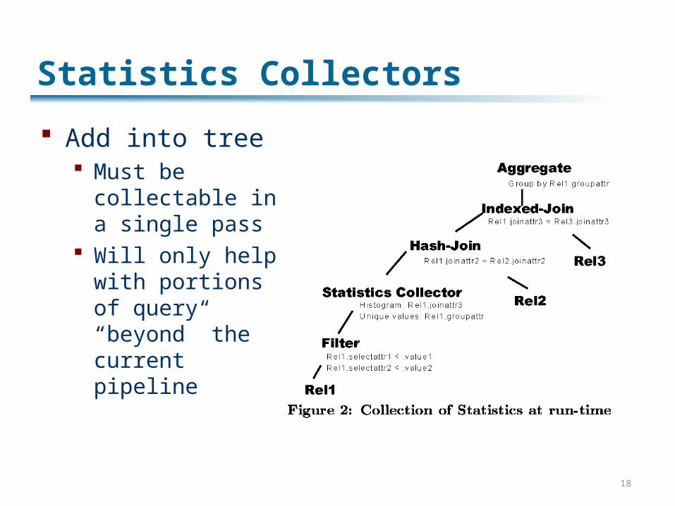
Statistics Collectors

Add into tree Must be

collectable in a single pass

Will only help with portions of query “beyond” the current pipeline

19

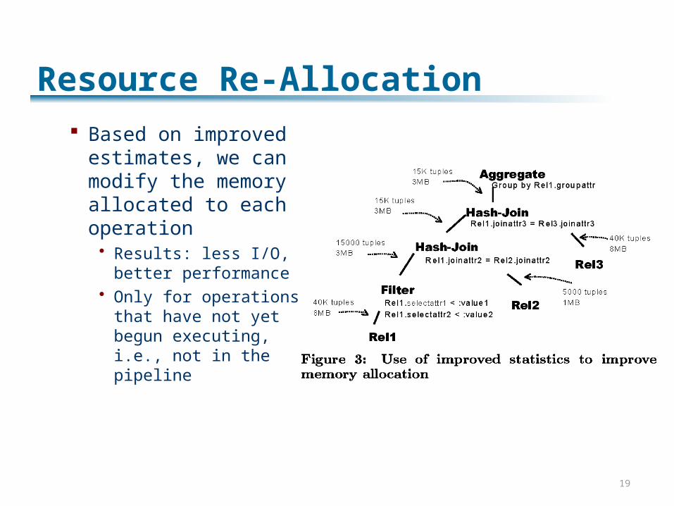
Resource Re-Allocation Based on improved

estimates, we can modify the memory allocated to each operation Results: less I/O,

better performance Only for operations

that have not yet begun executing, i.e., not in the pipeline

20

Plan Modification

Only re-optimize part not begun

Suspend query, save intermediate in temp file

Create new plan for remainder, treating temp as an input

21

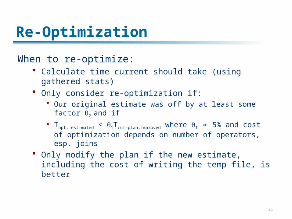
Re-Optimization

When to re-optimize: Calculate time current should take (using gathered

stats) Only consider re-optimization if:

Our original estimate was off by at least some factor 2 and if

Topt, estimated < 1Tcur-plan,improved where 1 5% and cost of optimization depends on number of operators, esp. joins

Only modify the plan if the new estimate, including the cost of writing the temp file, is better

22

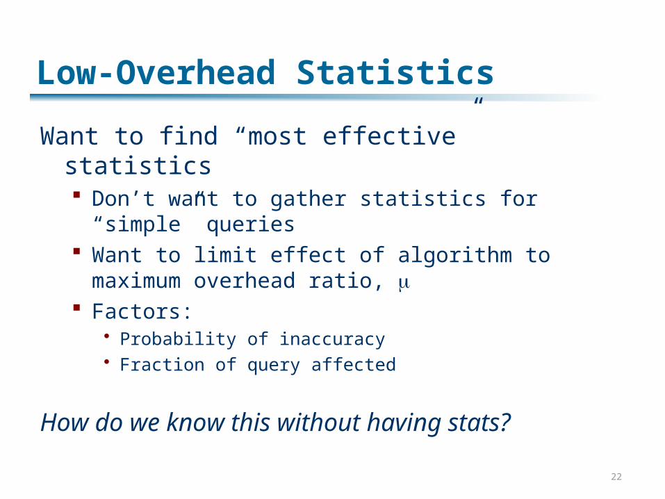
Low-Overhead Statistics

Want to find “most effective” statistics Don’t want to gather statistics for “simple”

queries Want to limit effect of algorithm to maximum

overhead ratio, Factors:

Probability of inaccuracy Fraction of query affected

How do we know this without having stats?

23

Inaccuracy Potentials

The following heuristics are used: Inaccuracy potential = low, medium, high Lower if we have more information on table

value distribution 1+max of inputs for multiple-input selection Always high for user-defined methods Always high for non-equijoins For most other operators, same as worst of

inputs

24

More Heuristics

Check fraction of query affected Check how many other

operators use the same statistic

The winner: Higher inaccuracy

potentials first Then, if a tie, the one

affecting the larger portion of the plan

25

Implementation

On top of Paradise (parallel database that supports ADTs, built on OO framework)

Using System-R optimizer New SCIA (Stat Collector Insertion Algorithm)

and Dynamic Re-Optimization modules

26

It Works!

Results are 5% worse for simple queries, much better for complex queries Of course, we would not really collect statistics on

simple queries Data skew made a slight difference - both normal

and re-optimized queries performed slightly better

27

Pros and Cons

Provides significant potential for improvement without adding much overhead Biased towards exploitation, with very limited information-

gathering

A great way to retrofit an existing system In SIGMOD04, IBM had a paper that did this in DB2

But fairly limited to traditional DB context Relies on us knowing the (rough) cardinalities of the sources Query plans aren’t pipelined, meaning:

If the pipeline is broken too infrequently, MQRO may not help If the pipeline is broken too frequently, time-to-first-answer is

slow

28

The Opposite Extreme: Eddies

The basic idea: Query processing consists of sending tuples through

a series of operators Why not treat it like a routing problem? Rely on “back-pressure” (i.e., queue overflow) to tell

us where to send tuples

Part of the ongoing Telegraph project at Berkeley Large-scale federated, shared-nothing data stream

engine Variations in data transfer rates Little knowledge of data sources

29

Telegraph Architecture

Simple “pre-optimizer” to generate initial plan Creates operators, e.g.:

Select: predicate(sourceA) Join: predicate(sourceA, sourceB) (No support for aggregation, union, etc.)

Chooses implementationsSelect using index, join using hash join

Goal: dataflow-driven scheduling of operations Tuple comes into system Adaptively routed through operators in “eddies”

May be combined, discarded, etc.

30

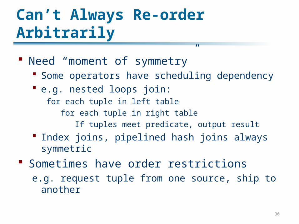
Can’t Always Re-order Arbitrarily

Need “moment of symmetry” Some operators have scheduling dependency e.g. nested loops join:

for each tuple in left tablefor each tuple in right table

If tuples meet predicate, output result

Index joins, pipelined hash joins always symmetric

Sometimes have order restrictionse.g. request tuple from one source, ship to

another

31

The Eddy

Represents set of possible orderings of a subplan

Each tuple may “flow” through a different ordering (which may be constrained)

N-ary module consisting of query operators Basic unit of adaptivity

Subplan with select, project, join operators

U

32

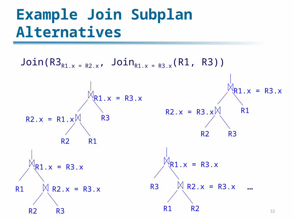
Example Join Subplan Alternatives

R2 R1

R2.x = R1.x R3

R1.x = R3.x

R2 R3

R2.x = R3.x R1

R1.x = R3.x

R2 R3

R2.x = R3.xR1

R1.x = R3.x

R1 R2

R2.x = R3.xR3

R1.x = R3.x

…

Join(R3R1.x = R2.x, JoinR1.x = R3.x(R1, R3))

33

Naïve Eddy

Given tuple, route to operator that’s ready Analogous to fluid dynamicsAdjusts to operator costs Ignores operator selectivity (reduction of input)

34

Adapting to Variable-Cost Selection

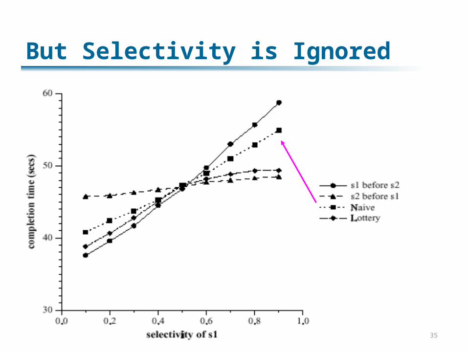
35

But Selectivity is Ignored

36

Lottery-Based Eddy

Need to favor more selective operators Ticket given per tuple input, returned per

output Lottery scheduling based on number of ticketsNow handles both selectivity and cost

37

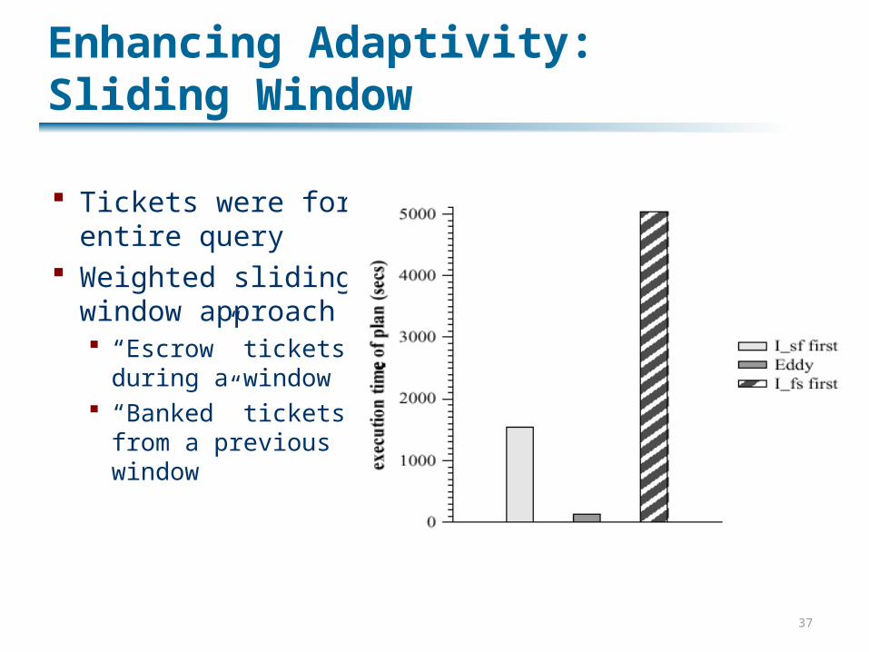
Enhancing Adaptivity: Sliding Window

Tickets were for entire query

Weighted sliding window approach “Escrow” tickets

during a window “Banked” tickets

from a previous window

38

What about Delays?

Problems here:Don’t know when join buffers vs. “discards” tuples

S R (SLOW)

T

39

Eddy Pros and Cons

Mechanism for adaptively re-routing queries Makes optimizer’s task simpler Can do nearly as well as well-optimized plan in

some cases Handles variable costs, variable selectivities

But doesn’t really handle joins very well – attempts to address in follow-up work: STeMs – break a join into separate data

structures; requires re-computation at each step STAIRs – create intermediate state and shuffle it

back and forth

40

Other Areas Where Things Can be Improved

The work of pre-optimization or re-optimization Choose good initial/next query plan Pick operator implementations, access methods

STeMs fix this

Handle arbitrary operatorsAggregation, outer join, sorting, …Next time we’ll see techniques to address this

Distribute work Distributed eddies (by DeWitt and students)