mini tab 14 one day training 39403
TRANSCRIPT

Minitab 14 Quality Statistics
A person without data is merely expressing an opinion….
Created by Paul White - Aston Martin Six Sigma Department

2
Introduction
Name
Department
Six Sigma / Minitab experience
Why are you here today?

3
Training Topics
What is Six Sigma? Introduction to Minitab Version 14 Manipulation of data Basic statistics Graphs Quality tools Measurement System Analysis – R & R Control charts Normality testing Capability analysis Hypothesis Testing

What is Six Sigma?
‘The function of a statistician is to make predictions, and thus to provide a basis for action’ – W.E Deming

5
6-Sigma99.99966% Good
6-Sigma99.99966% Good
• Seven articles lost per hour• 20,000 lost articles of mail per hour
3.8-Sigma99% Good3.8-Sigma99% Good
• Unsafe drinking water for almost 15 minutes each day
• Unsafe drinking water one minute every seven months
• 5,000 incorrect surgical operations per week
• 1.7 incorrect operations per week
• 1 missed putt per 9 holes of golf • 1 missed putt per 163 years
• 10,700 defects per million opportunities
• 3.4 defects per million opportunities
Is 99% Good Enough?

6
Goals of Six Sigma
Reduce defects.
Improve process capability.
Improve customer satisfaction.
Increase shareholder value.
This ensures we are competitive, provides future security and opportunity for growth.

7
100% Inspection – Does it work?
100% Inspection

8
Finished files are the results of many years of sceintific studies combined with the experience of many years of
effort
F-Test

9
How many did you see?
Have another look!
F-Test

10
Finished files are the results of many years of sceintific studies combined with the experience of many years of
effort
F-Test

11
Did anyone change their mind?
F-Test

12
Finished files are the results of many years of sceintific studies combined with the experience of many years of
effort
F-Test

13
Did you spot anything else?
F-Test

14
Finished files are the results of many years of sceintific studies combined with the experience of many years of
effort
F-Test
F-Test

15
100% Inspection – Does it work?
100% Inspection

16
DMAIC Improvement Model
Introduction to Minitab
‘Statisticians are people with tears wiped from their eyes’

18
Introduction to Minitab
The 3 Minitab views - session folder, worksheet folder, project folder.
3 types of data entry– numbers, text and dates.
Importing text from other sources
Creating, opening and saving projects and worksheets.

19
Session and Worksheet Folders
The 2 main windows in Minitab – The session folder & worksheet folder.
Session folder
Worksheet folder
Select different views using icons

20
Project Folder
Multiple worksheets can be opened within the same project.
File /New / New worksheet
Multiple worksheets
Select project manager

21
3 Types of data
Minitab stores numbers, text and dates.
Numbers – No symbol in column header, right aligned in cell
Text – T in column header, left aligned in cell
Date – D in column header, left aligned in cell

22
Numeric Data Types
FAIL PASS
Electrical Circuit
TEMPERATURE
Thermometer
TimeTime
VariableAttribute
NO-GO GO
Caliper
QTY UNIT DESCRIPTION TOTAL
1 $10.00 $10.00
3 $1.50 $4.50
10 $10.00 $10.00
2 $5.00 $10.00
SHIPPING ORDER
Error

23
Attribute vs Variable Data
Variable
Attribute
The Advantage of Variable Data
29

24
Attribute vs Variable Data
Variable Data Available earlier in the process, before defects occur. Illustrates short term trends allowing immediate action. A small amount of data is required to draw conclusions
(minimum 30 individual readings).
Attribute Data Defect related, only after the fault has occurred. Only illustrates long term trends. A large amount of data is required to draw conclusions
(minimum 50 subgroups) Sometimes this is the only data available.

25
Importing text from other sources
Easiest way is to copy & paste. However, an import function is available: File / other files / import special text.
Tip! Always title each column in the cell below the column reference number. this will make later analysis easier to interpret as the graphs will include your column description.
Select destination cell in Minitab and paste from clipboard
Select data from another source (such as Excel) and copy to clipboard.

26
Saving projects and worksheets
Save projects to correct destination.
File / Save project as
Change default saving location
Rename with relevant filename and date

Manipulating Data
‘Facts are stubborn things, but statistics are more pliable’

28
Manipulating Data
Erasing columns and rows
Stacking columns and rows
Transposing columns

29
Erasing data
Erasing columns and rows
Select column and right click mouse
Delete cells
Tip! Undo function is available on the toolbar

30
Stacking columns
Data / Stack / Stack Columns
Select columns to stack
Select stacked destination and subscripts
Click OK
Tip! Always store subscripts when stacking data, this will copy the column description to the adjacent data cell. This makes future analysis easier, to discriminate between data sets.

31
Transposing data
Data / Transpose columns
Switch the data pattern from columns to rows.
Select columns to transpose
Select destination option
Tip! If your data is already in Excel you can use the ‘paste special’ function to transpose from columns to rows and vice versa! Use Minitab & Excel interchangeably to conduct data analysis.
Click OK

Basic Statistics
‘Statistics should be used the way a drunk uses a lamp post, more for support than enlightenment ’

33
Basic Statistics
Descriptive statistics
Inferential statistics
Graphical summary

34
Descriptive Statistics
Stat / Basic statistics / display descriptive statistics.
Stat /Basic statistics / Display descriptive statistics
Select variables, click OK

35
Descriptive Statistics
Descriptive statistics describe the sample we have gathered, tells us what is.
Session window output

36
Measures of Average
Mean:Calculated average. Sum of all individual values, divided by the number of samples.
Mode: Most frequently occurring value.
Median: The middle number when the values are sequentially arranged.

37
Mean =
Mean
5, 5, 4, 2, 1,1, 4, 5, 3, 2.
Measures of Average
3.2

38
5, 5, 4, 2, 1,1, 4, 5, 3, 2.
Measures of Average
Mode =
Mode
5

39
Median =
Median
5, 5, 4, 2, 1,1, 4, 5, 3, 2.
Measures of Average

40
1, 1, 2, 2, 3, 4, 4, 5, 5, 5.
Median = 3.5
3+4 2 = 3.5
Median
Measures of Average

41
Mean =3.2Mode =5Median =3.5
5, 5, 4, 2, 1,1, 4, 5, 3, 2.
Measures of Average

42
Graphical Summary
Stat / Basic statistics / Graphical summary.
Stat / Basic Statistics / Graphical Summary
Select variable
Click OK
Tip! Note the confidence level of 95% in the option window. This applies to the inferential statistics that will be displayed in the graphical summary.

43
Graphical Summary
Descriptive statistics describe the sample we have gathered, tells us what is. Inferential statistics allows us to “infer” about the population, tells us what
“probably is”. Inferences are never definite, only stated with a degree of confidence.
Normality test
Descriptive statistics
Inferential statistics
10.810.410.09.6
Median
Mean
10.1510.1010.0510.009.959.90
1st Quartile 9.800
Median 10.0253rd Quartile 10.240Maximum 10.839
9.922 10.105
9.915 10.126
0.268 0.400
A-Squared 0.19
P-Value 0.902
Mean 10.014StDev 0.321Variance 0.103
Skewness -0.003050Kurtosis -0.106782N 50
Minimum 9.310
Anderson-Darling Normality Test
95% Confidence I nterval for Mean
95% Confidence I nterval for Median
95% Confidence I nterval for StDev95% Confidence I ntervals
Summary for Tool 1

44
High Standard DeviationHigh Variability
Low Standard DeviationLow Variability
Standard Deviation
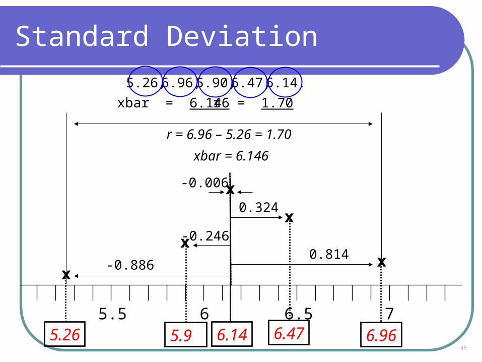
Standard Deviation refers to the collective deviation of the entire data set
45
6.1465.5 6.5 7
xx
x
x
x
5.26
xbar = 6.146
6.965.9 6.47
xbar = 6.146
-0.8860.814
-0.246
0.324
-0.006
5.26,6.96,5.90,6.47,6.14.
r = 6.96 – 5.26 = 1.70
r = 1.70
Standard Deviation

46
Calculating standard deviation is best shown in table format: (xbar = 6.146)
Data x - xbar (x – xbar)2
5.26
6.96
5.90
6.47
6.14
-0.886 0.7849960.814
-0.246
0.324
-0.006
0.662596
0.060516
0.104976
0.000036
= 1.61312S = (x – X)2
n - 1√_
Standard Deviation

47
S = (x – X)2
n - 1√_
S = 1.613124√
S = 0.40328√S = 0.635 (to 3 s.f.)
We can now use the formula:
Standard Deviation
Tip! The square of the standard deviation is the variance.

48
The distribution of area as a percentage:
-3s -2s -1s X +1s +2s +3s
68.26%
95.44%
99.73%
0.135%
0.135%
Normal Distribution

49
Graphical Summary
Descriptive statistics describe the sample we have gathered, tells us what is. Inferential statistics allows us to “infer” about the population, tells us what
“probably is”. Inferences are never definite, only stated with a degree of confidence.
Normality test
Descriptive statistics
Inferential statistics
10.810.410.09.6
Median
Mean
10.1510.1010.0510.009.959.90
1st Quartile 9.800
Median 10.0253rd Quartile 10.240Maximum 10.839
9.922 10.105
9.915 10.126
0.268 0.400
A-Squared 0.19
P-Value 0.902
Mean 10.014StDev 0.321Variance 0.103
Skewness -0.003050Kurtosis -0.106782N 50
Minimum 9.310
Anderson-Darling Normality Test
95% Confidence I nterval for Mean
95% Confidence I nterval for Median
95% Confidence I nterval for StDev95% Confidence I ntervals
Summary for Tool 1

Graphs
‘A picture tells a 1,000 words’

51
Graphs
Time series plot
Histogram
Boxplot
Editing graphs
Update graphs in real time

52
Time Series Plot
Graph / Time series plot
Graph / Time Series Plot
Select simple option
Tip! Minitab 14 allows multiple time series plots on one chart if required!

53
Time Series Plot
Graph / Time series plot
Select variable to plot
Select time scale
Select stamp
Select stamp column
Click OK

54
Time Series Plot
Time series plot displays the trend over time
Date
Tool 1
19/0
2/20
06
14/0
2/20
06
09/0
2/20
06
04/0
2/20
06
30/0
1/20
06
25/0
1/20
06
20/0
1/20
06
15/0
1/20
06
10/0
1/20
06
05/0
1/20
06
01/0
1/20
06
11.0
10.5
10.0
9.5
Time Series Plot of Tool 1

55
Histogram
Graph / Histogram.
Graph / Histogram
Select simple option

56
Histogram
Graph / Histogram.
Select variable to graph
Click OK

57
Histogram
A histogram shows the distribution of the data.
Tool 1
Frequency
10.810.610.410.210.09.89.69.4
16
14
12
10
8
6
4
2
0
Histogram of Tool 1
Tip! When copying graphs into other file formats, such as the 6 Panel template. Use edit / paste special and paste the graph as a picture to reduce the file size.

58
Boxplot
Graph / Boxplot
Graph / Boxplot
Select Multiple Y’s - Simple Option

59
Boxplot
Graph / Boxplot
Select variables
Click OK

60
Data
Tool 3Tool 2Tool 1
14
13
12
11
10
9
8
7
6
Boxplot of Tool 1, Tool 2, Tool 3
Boxplot
A boxplot is a ‘birds eye view’ of a histogram.
Whisker
Inter quartile range – middle 50%
Median
Tip! A boxplot is a very good tool to compare multiple distributions.

61
Editing Graphs
Minitab 14 allows advanced graphical editing features.
Double click graph on area to be edited (as per Excel approach)
Use options box to edit graphical features

62
Editing Graphs
Minitab 14 allows advanced graphical editing features.Data
Tool 3Tool 2Tool 1
14
13
12
11
10
9
8
7
6
Boxplot of Tool 1, Tool 2, Tool 3
63
Update Graphs in Real Time
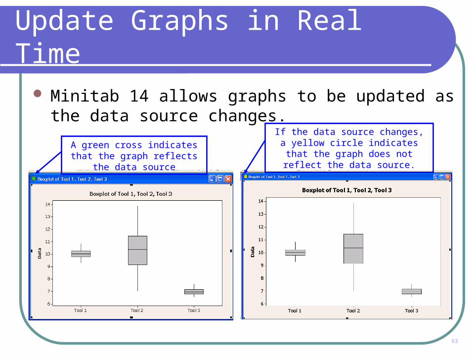
Minitab 14 allows graphs to be updated as the data source changes.
A green cross indicates that the graph reflects the data source
If the data source changes, a yellow circle indicates that the graph does
not reflect the data source.

64
Update Graphs in Real Time
Graphs can be updated automatically or upon request.
Right click graph and select update graph now

65
Update Graphs in Real Time
A green cross indicates that the graph has been updated.
Tip! The update graph function can be used on all graphs in the graph menu (except stem & leaf) and all control charts!

Quality Tools
‘Statistics may be defined as a body of methods for making wise decisions in the face of uncertainty ’ – W.A.Wallis

67
Quality Tools
Pareto chart
Cause and Effect Diagram
Multi-Vari Chart

68
Quality Tools
Stat / Quality Tools / Pareto chart
Select columns for labels and frequencies
Click OK
Stat / Quality Tools / Pareto Chart

69
Quality Tools
Pareto charts are based on the 80 / 20 rule. Used to prioritise focus.
Cumulative frequency
Faults
Results
Tip! Pareto charts should also be produced using COPQ for each defect.
Count 19 17 15100 39 25 23 22 21 20 20Percent 5.9 5.3 4.731.2 12.1 7.8 7.2 6.9 6.5 6.2 6.2Cum % 90.0 95.3 100.031.2 43.3 51.1 58.3 65.1 71.7 77.9 84.1
Count
Perc
ent
Characteristic
Oth
er
Fas
cia
- P
oor
Fit
Glo
veb
ox
poor
fit
Pai
nt D
efec
t -
LH d
oor
Fla
t bat
tery
Rea
r bum
per
poor
fit
Wat
er le
ak R
r D
oor
Cam
ber
adju
stm
ent
Win
d n
oise
Frt
Door
Air V
ent Poor
Fit
Wid
get
350
300
250
200
150
100
50
0
100
80
60
40
20
0
Pareto Chart of Characteristic

70
Cause & Effect Diagram
Conduct team brainstorm Stat / Quality tools / Cause & Effect Diagram
Stat / Quality Tools / C&E Diagram
Enter causes in columns or text
Click OK
Tip! Use 5 why analysis to drill down to root cause. Minitab 14 allows multiple sub branches to be entered in the option box.

71
Cause & Effect Diagram
Use C&E to understand relationship between inputs and outputs.
Tip! The Six Sigma team should score the relationship between inputs & outputs using the C&E matrix to prioritise team focus.
DistortionPanel
Environment
Measurements
Methods
Material
Machines
Personnel
Poor training
Material Handling
New Labour
Shims missing
Location peg damage
Wear on tool
Damaged panels
Panel dimensions
Burr on panel
Standardised Work
Stock Rotation
Build sequence
procedureNo measurement
No gauge R&R
Gauge calibration
Poor lighting
Temperature
Humidity
BIW Door Panel

72
Multi-Vari Chart
Graphical analysis of means for different factors. Stat / Quality tools / Multi-Vari Chart
Stat / Quality Tools / Multi-Vari Charts
Enter response variable (y) and factor levels (x)

73
Multi-Vari Chart
Stat / Quality tools / Multi-Vari Chart
Mean values displayed for each factor level
Multi-Vari charts can be used during a screening DOE to reduce KPIV’s to the ‘critical few’.
Displays main effects and interactions.
Tool Number
Torq
ue
321
56
55
54
53
52
51
50
49
48
Atlas CopcoBosch
Supplier
Multi-Vari Chart for Torque by Supplier - Tool Number

Measurement Systems Analysis
‘When you can measure what you are talking about and express it in numbers, you know something about it. But, when you cannot express it in numbers, your knowledge is of the meagre and unsatisfactory kind’ – Lord Kelvin

75
Measurement Systems Analysis
MSA Overview
Attribute Gauge R&R
Variable Gauge R&R

76
The purpose of Measurement System Analysis (MSA) is to ensure the information collected is a true representation of what is occurring in the process.
MSA is the evaluation of measurement system variation in comparison to process variation.
Measurement System Analysis
MSA validation is required before commencing data collection.
Process Variation
Measurement System Variation

77
Measurement System Analysis
R & R – Repeatability and reproducibility.
Repeatability refers to the inherent variability of the measurement system.
Same operatorSame partSame condition
Repeatability is the ‘within’ variation.

78
Measurement System Analysis
R & R – Repeatability and reproducibility.
Reproducibility refers to the variation that occurs when different conditions are used to take the measurement.
Different operatorDifferent partsDifferent conditions
Reproducibility is the ‘between’ variation.
79
Measurement System Analysis
R & R – Repeatability and reproducibility.
Reproducibility refers to the variation that occurs when different conditions are used to take the measurement.
Different operatorDifferent partsDifferent conditions
Reproducibility is the ‘between’ variation.

80
Data Types
FAIL PASS
Electrical Circuit
TEMPERATURE
Thermometer
TimeTime
VariableAttribute
NO-GO GO
Caliper
QTY UNIT DESCRIPTION TOTAL
1 $10.00 $10.00
3 $1.50 $4.50
10 $10.00 $10.00
2 $5.00 $10.00
SHIPPING ORDER
Error

81
Attribute Gauge R & R Exercise
Scenario The process to stamp dots on a domino is highly variable. RFT data is required to evaluate process performance. Measurement system must be validated first.
Study Method 2 operators 2 measurements per operator 7 samples
N.B Only 7 samples used due to time constraints. A minimum of 30 samples required for Six Sigma projects.

82
Attribute Gauge R & R Exercise
Measurement Procedure No. 1
Visually inspect all dominoes to identify samples with dots smaller than the master sample.
Any non-conformance is considered a reject. Colour is of no consequence.
You have been allocated 15 seconds to inspect each sample.

83
Attribute Gauge R & R Exercise
75
Is the measurement system repeatable and reproducible?
What can be done to improve the measurement system?

84
Attribute Gauge R & R Exercise
Measurement Procedure No. 2
Inspect all dominoes with the gauge provided. Ensure there are no spots smaller than the master sample. Any non-conformance is considered a reject. Colour is of no consequence.
You have been allocated 30 seconds to inspect each sample.

85
Attribute Gauge R & R Exercise
Stat / Quality Tools / Attribute Agreement Analysis
Select data, samples and appraisers
Stat / Quality Tools / Attribute Agreement Analysis Enter study
information
Click OK

86
Attribute Gauge R & R Output
Attribute Gage R&R StudyAttribute Gage R&R Study for Result
Within AppraiserAssessment Agreement
Appraiser # Inspected # Matched Percent (%) 95.0% CI Eric 7 7 100.0 ( 65.2, 100.0)John 7 7 100.0 ( 65.2, 100.0)
# Matched: Appraiser agrees with him/herself across trials.
Between AppraisersAssessment Agreement
# Inspected # Matched Percent (%) 95.0% CI 7 7 100.0 ( 65.2, 100.0)
# Matched: All appraisers' assessments agree with each other.
Graphical Output Session Window
Graph displays actual % result and 95% confidence interval Session window displays detailed results
Appraiser
Pe
rce
nt
J ohnEric
100
80
60
40
20
0
95.0% CIPercent
Date of study: 13/10/2006Reported by: Paul WhiteName of product: BIW Panel Distortion
Assessment Agreement
Within Appraisers
Tip! A Kappa statistic is available to determine correlation within & between appraisers.

87
Attribute Gauge R & R Summary
A ‘typical’ Attribute Gauge R&R Study includes: 1 to 3 operators (measurement takers) 30 samples 2 to 3 trials (measurements) of each sample by each operator Samples that are typical of the process (pass & fail)
An acceptable study is where 100% agreement between each operator and the Master Attribute has been achieved (if a Master Attribute is included).
Analysis of the results from a failed study can identify where improvements need to be made: Operator training Standardised inspection process Measurement Procedure

88
Variable Gauge R & R
R&R studies are conducted to ensure the data collected is a true representation of what is occurring in the process.
The purpose of variable gauge R&R studies are to calculate the amount of measurement system variation in comparison to the process variation and the process tolerance.
A ‘typical’ variable gauge R&R Study includes: 1 to 3 operators (measurement takers) 10 samples 2 to 3 trials (measurements) of each sample by each
operator Samples that are typical of the process (in spec & out of
spec)

89
ScenarioScenarioGandalf’s Castle has been under siege from the Orcs for several days
and he seems to be losing the battle. The main problem is that Gandalf’s long range weapons – the catapults
– keep missing the Orcs who are sheltering behind a ridge 200m away. They keep shooting either too long or too short.
Gandalf wants to improve the accuracy of his catapults.But, before he can improve the accuracy Gandalf must ensure he can
measure the distance repeatedly & reproducibly.
ExerciseConduct variable r&r study on catapult shot length.10 shots (or samples), 2 operators, 2 measurements per operatorRecord results on flip chart.
Variable Gauge R & R Exercise

90
Variable Gauge R & R Exercise
Stat / Quality Tools / Gage Study / Gage R&R Study (Crossed)
Stat / Quality Tools / Gage Study / Gage R&R Study (Crossed)
Tip! A Nested Gage R&R Study is available for a destructive measurement study.

91
Variable Gauge R & R Exercise
Stat / Quality Tools / Gage Study / Gage R&R Study (Crossed)
Enter part no. Operator & Measurement Data
Tip! Always enter the process tolerance via the options box. It is imperative to compare measurement system variation against the process variation & the process tolerance.

92
Gage R&R Study – ANOVA Method
Gage name: Tin Foil
Reported by: Paul White
Date of study: 16th February 2006
Tolerance: 0 +/-0.05
%Contribution
Source Variance (of Variance)
Total Gage R&R 19.62 1.59
Repeatability 17.73 1.44
Reproducibility 1.89 0.15
Part-to-Part 1212.92 98.41
Total Variation 1232.55 100.00
StdDev Study Var %Study Var
Source (SD) (5.15*SD) (%SV)
Total Gage R&R 4.4299 22.814 12.62
Repeatability 4.2110 21.687 11.99
Reproducibility 1.3752 7.082 3.92
Part-to-Part 34.8270 179.359 99.20
Total Variation 35.1076 180.804 100.00
Number of distinct categories = 11
Variable R & R Pass Criteria
% Study Variation must be < 30%
% Contribution must be < 9%
Distinct categories must be >=5
Tip! Gauge calibration does not negate the requirement to conduct an MSA. Calibration confirms the gauge is accurate, MSA ensures the whole measurement system is repeatable and reproducible.

93
Variable R&R – Pass Criteria % Contribution% Contribution
Measurement Measurement System Variation as a percentage of Total Observed Process Variation (Variance)
% Study Variation % Study Variation
MMeasurement System Standard Deviation as a percentage of Total Observed Process Standard Deviation (using Standard Deviation)
% Tolerance % Tolerance
MMeasurement Error as a percentage of Tolerance
Number of Distinct Categories Number of Distinct Categories
Less Less than 5 indicates Attribute conditions
% Contribution % Study Variation (Process Control)
% Tolerance (Product Control) # of Distinct Categories
It is desirable to have ALL indicators Green
RR
YY
GG < 1% Good
2-9% Acceptable
> 9% Unacceptable RR
YY
GG < 10% Good
11-30% Acceptable
> 30% Unacceptable RR
YY
GG < 10% Good
11-30% Acceptable
> 30% Unacceptable RR
YY
GG > 10 Good
5-10 Acceptable
< 5 Unacceptable

94
Per
cent
Part-to-PartReprodRepeatGage R&R
100
50
0
% Contribution
% Study Var
Sam
ple
Ran
ge
30
15
0
_R=5.3
UCL=17.32
LCL=0
1 2
Sam
ple
Mea
n
200
100
0
__X=99.5UCL=109.4LCL=89.5
1 2
Part54321
200
100
0
Operator21
200
100
0
Part
Ave
rage
54321
200
100
0
1
2
Operator
Gage name: VernierDate of study: 13/06/2006
Reported by: Paul WhiteTolerance: N/A
Components of Variation
R Chart by Operator
Xbar Chart by Operator
Measurement by Part
Measurement by Operator
Operator * Part Interaction
Gage R&R (ANOVA) for Measurement
Variable R & R Diagnostic Graphs
Review the diagnostic graphs to identify sources of measurement system variation.
Overall health of Measurement System
Repeatability
Reproducibility
Repeatability & gauge linearity
Reproducibility across operators
Reproducibility across parts

95
Catapult MSA
Analyse MSA data collected from catapult
Discuss results with team
Present findings to class

96
Variable Gauge R & R Summary
A ‘typical’ Variable Gauge R&R Study includes: 1 to 3 operators (measurement takers) 10 samples 2 to 3 trials (measurements) of each sample by each operator Samples that are typical of the process.
An acceptable study is where the total gauge R&R is less than 30% of the process spread or tolerance.
Distinct categories must be > = 5.
Analysis of the results from a failed study can identify where improvements need to be made: Standardised inspection process Operator training Measurement Procedure

97
Summary – MSA
At conclusion of the MSA, the Six Sigma team should know:
The measurement system is capable of gathering data that accurately reflects variation in the process.
If there is measurement error, how big it is and a method of accounting for it.
Measurement increments are small enough to show variation.
Sources of measurement error have been identified

Control Charts
‘Statistics is not a discipline like physics, chemistry or biology where we study a subject to solve problems in the same subject. We study statistics with the main aim of solving problems in other disciplines." - C.R. Rao

99
Control Charts
Introduction to Control Charts
Control Limits
In Control
Out of Control
Attribute control charts
Variable control charts

100
Control Charts
A control chart is a run chart with upper and lower control limits (not specification limits).
Control charts are used to detect and monitor process variation over time.
Distinguishes between special and common cause.
Data must be collected in ‘real time’.
It is important to record the ‘voice of the process’. Ensure all process events / changes are logged.
Can be used as a reference point to evaluate the impact of process changes.
Serves as a tool for ongoing control.

101
Control Limits
1
2
3
4
5
7
8
9
Average +/- 3 S.D
99.73%
Upper Control Limit
Lower Control Limit
Control limits are calculated from the data from the process.
Control limits are not specification limits!

102
In Control
A process is in control when all of the values are randomly spread between the control limits.
To be in control means the process is consistent.
1
2
3
4
5
7
8
9
1
2
3
4
5
7
8
9

103
Out of Control
A process is out of control when one value exceeds the control limits.
This is special cause variation.
1
2
3
4
5
7
8
9
1
2
3
4
5
7
8
9

104
Out of Control
A process is out of control when 9 readings fall on one side of the process average but inside the control limits.
This out of control condition indicates a process shift.
1
2
3
4
5
7
8
9
1
2
3
4
5
7
8
9

105
Out of Control
A process is out of control when 6 readings in a row, display a continuous trend in an upward or downward direction.
This out of control condition indicates process drift / wear.
1
2
3
4
5
7
8
9
1
2
3
4
5
7
8
9
5566
SPC charts require ‘real time’ data collection.

106
Out of Control Rules
Tools / Options / Control Charts / Define Tests
Tip! Minitab uses Nelson’s Test for Special Cause as they improved on the Western Electric Rules by aligning the probabilities of false alarm rates.
Tests for special cause
Tools / Options/ Control Charts / Define Tests
107
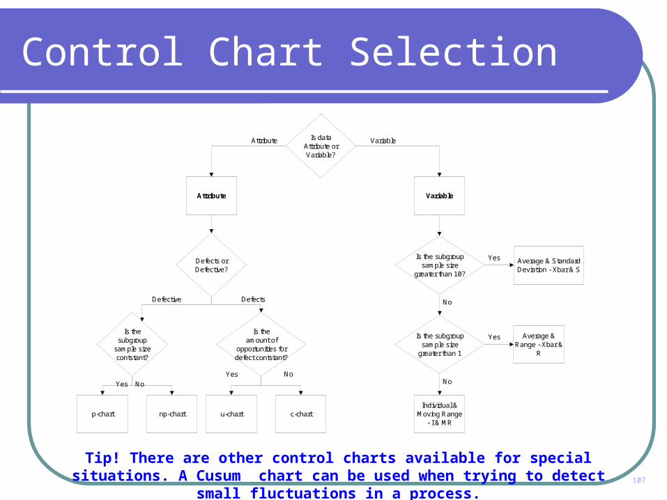
Start
Is data Attribute or Variable?
Attribute Variable
Defects or Defective?
Is the subgroup
sample size contstant?
Is theamount of
opportunities for defect contstant?
p-chart np-chart u-chart c-chart
Is the subgroup sample size
greater than 10?
Is the subgroup sample size
greater than 1
Individual & Moving Range
- I & MR
Average & Range - Xbar &
R
Average & Standard Deviation - Xbar & S
Yes
No
No
Yes
Yes
NoNoYes
Attribute Variable
Defective Defects
Control Chart Selection
Tip! There are other control charts available for special situations. A Cusum chart can be used when trying to detect small fluctuations in a process.

108
P Chart
Stat / Control Charts / Attribute Charts / P-Chart
Select column with defective amounts
Tip! Use the scale options to display the date on the chart x-axis.
Select column with subgroup sample sizes in. I.e. Daily or weekly volume
Select OK
Stat / Control Charts / Attribute Charts/ P-Chart

109
P Chart
A P Chart displays the proportion defective.
Tip! The P Chart is based on the Binomial distribution – pass or fail.
Date
Pro
port
ion
09/0
2/20
06
07/0
2/20
06
05/0
2/20
06
03/0
2/20
06
01/0
2/20
06
30/0
1/20
06
28/0
1/20
06
26/0
1/20
06
24/0
1/20
06
22/0
1/20
060.4
0.3
0.2
0.1
0.0
_P=0.1097
UCL=0.2338
LCL=0
1
P Chart of No of cars with Defective Vent
Tests performed with unequal sample sizes

110
U Chart
Stat / Control Charts / Attribute Charts / U-Chart
Click OK
Select column with defects data
Select column with subgroup sample sizes in. I.e. Daily or weekly volume
Stat / Control Chart / Attribute Charts / U Chart

111
U Chart
A U Chart displays the no of defects per unit.
Tip! The U Chart is based on the Poisson distribution – how many defects per item.
Date
Sam
ple
Count
Per
Unit
09/0
2/20
06
07/0
2/20
06
05/0
2/20
06
03/0
2/20
06
01/0
2/20
06
30/0
1/20
06
28/0
1/20
06
26/0
1/20
06
24/0
1/20
06
22/0
1/20
060.6
0.5
0.4
0.3
0.2
0.1
0.0
_U=0.1300
UCL=0.2732
LCL=0
1
U Chart of No of Air Vents Defects
Tests performed with unequal sample sizes
Unequal subgroup sample sizes will create castellated control limits

112
Variable Control Charts
Accuracy describes
Centering
Precision describesSpread

113
Individual & Moving Range Chart
Stat / Control Chart / Variables for Individuals / I&MR
Tip! Always title your chart using the Labels option box. All charts should have a title to aid reader interpretation.
Select column with measurement data
Click OK
Stat / Control Chart/ Variables for Individuals / I&MR

114
Individual & Moving Range Chart
I & MR chart shows the trend of individual data readings over time.
Tip! I & MR charts should be used to control process parameters (something that does not leave with the vehicle) I.e. Oven temperature, humidity, etc.
Displays the trend over time of individual readings. This part of the chart shows the accuracy of the process .
Displays the difference between consecutive readings. This part of the chart shows the precision of the process .
Date
Indiv
idual V
alu
e
15/02/200610/02/200605/02/200631/01/200626/01/200621/01/200616/01/200611/01/200606/01/200601/01/2006
11.0
10.5
10.0
9.5
9.0
_X=10.014
UCL=11.039
LCL=8.988
Date
Movin
g R
ange
15/02/200610/02/200605/02/200631/01/200626/01/200621/01/200616/01/200611/01/200606/01/200601/01/2006
1.2
0.9
0.6
0.3
0.0
__MR=0.386
UCL=1.260
LCL=0
I-MR Chart of Tool 1

115
Average & Range Chart
Stat / Control Chart / Variables for Sub-Groups / Xbar & R
Select column with measurement data
Click OK
Select subgroup size
Stat / Control Chart/ Variables for Sub-Groups / Xbar & R

116
Average & Range Chart
Xbar & R chart shows the average reading per subgroup over time.
Displays the trend over time of the subgroup average readings. This part of the chart shows the accuracy of the process .
Displays the range for each subgroup. I.e. Difference between the highest & lowest reading within each subgroup. This part of the chart shows the precision of the process .
Tip! Xbar & R charts should be used to control process characteristics (something that leaves with the vehicle) I.e. Gap condition on a door, thickness of paint, wheel alignment etc.
Sample
Sam
ple
Mean
10987654321
10.50
10.25
10.00
9.75
9.50
__X=10.014
UCL=10.458
LCL=9.569
Sample
Sam
ple
Range
10987654321
1.6
1.2
0.8
0.4
0.0
_R=0.770
UCL=1.629
LCL=0
Xbar-R Chart of Tool 1

117
Control Charts Summary
A control chart is a run chart with upper and lower control limits (not specification limits).
Control charts are used to detect and monitor process variation over time.
Distinguishes between special and common cause.
It is important to record the ‘voice of the process’. Ensure all process events / changes are logged.
Can be used as a reference point to evaluate the impact of process changes.
Serves as a tool for ongoing control.

Normality Test
‘Are statisticians normal?’

119
LSL Target USL
Normal Distribution
Normal Distribution
Data distribution characterized by a smooth, bell-shaped curve.

120
The distribution of area as a percentage:
-3s -2s -1s X +1s +2s +3s
68.26%
95.44%
99.73%
0.135%
0.135%
Normal Distribution

121
Normality Test
Stat / Basic statistics / Graphical summary.
Stat / Basic Statistics / Graphical Summary
Select variable
Click OK
Tip! Note the confidence level of 95% in the option window. This applies to the inferential statistics that will be displayed in the graphical summary.

122
Normality Test
Normality test
P-Value > 0.05 indicates a normal distribution
10.810.410.09.6
Median
Mean
10.1510.1010.0510.009.959.90
1st Quartile 9.800Median 10.0253rd Quartile 10.240Maximum 10.839
9.922 10.105
9.915 10.126
0.268 0.400
A-Squared 0.19P-Value 0.902
Mean 10.014StDev 0.321Variance 0.103Skewness -0.003050Kurtosis -0.106782N 50
Minimum 9.310
Anderson-Darling Normality Test
95% Confidence Interval for Mean
95% Confidence Interval for Median
95% Confidence Interval for StDev95% Confidence I ntervals
Summary for Tool 1
It is imperative to conduct a normality test when assessing variable data. The normal distribution is described by the mean and standard deviation (the
kurtosis & skewness provide additional info. about the shape of the curve). Control charts, process capability, 2 sample t-test and many other statistical
procedures are based on the normal distribution.

123
Typical Distributions
The shape has a bell shape.It is symmetric.
The shape has two humps.It is bimodal.
The shape has a long tail.It is not symmetric.
The shape is flat. There are one or more outliers.

124
Normality Test
Always conduct a normality test on variable data before conducting any statistical procedures.
I.e. Process capability, hypothesis testing etc.

Process Capability
‘A knowledge of statistics is like a knowledge of foreign languages or of algebra; it may prove of use at any time under any circumstances’

126
Process Capability
What is Process Capability?
Attribute Process Capability.
Variable Process Capability.
Sigma as a measure of capability.

127
Process Capability
Capability analysis is a measure of how well a process is meeting the expectations of the customer.
It provides a current performance baseline for the process.
It can be used as a reference point to evaluate the impact of process changes.
It can be displayed by several indices dependent on the data type.

128
VARIABLE DATA
Cp
Pp Ppk
Cpk
ATTRIBUTE DATA DPMODPUDPO
Capability Indices

129
Attribute Process Capability
50 readings are required to calculate attribute process capability.
Determine if failure mode is defective or a defect. Defective: Item is pass or fail. Defects: Item has multiple defects.
If item is defective use: Defects Per Million Opportunities (DPMO).
If defects per item are being assessed, use: Defects Per Unit (DPU).

130
DPMO
DPMO = Total number of defects
Total units Opportunities per unit 1,000,000
DPMO = 1,000,000D
N O
Calculate DPMO to identify baseline process capability. Unit (N) Defect (D) Opportunity (O) DPMO
DPMO ‘levels the playing field’ between different complexity processes.
I.e. The supplier of a bolt may only have 2 opportunities for failure whilst the supplier of the in-car entertainment system will have multiple opportunities due to a highly complex process.

131
DPMO in Minitab
Six Sigma / Product Report
Select Six Sigma / Product Report
Enter defects, units & opportunities
132
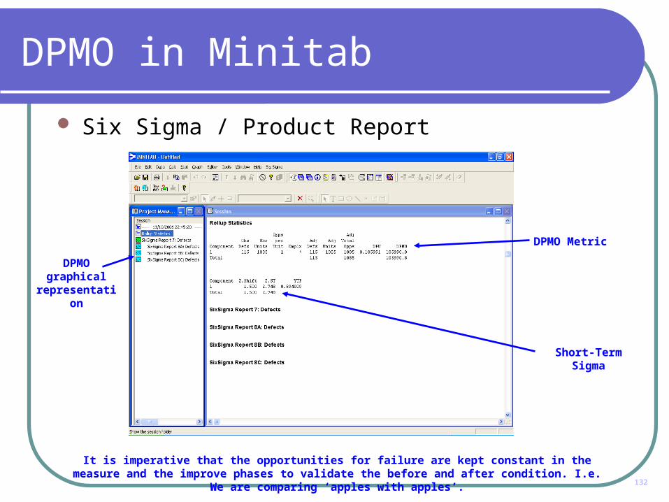
DPMO in Minitab
DPMO Metric
Six Sigma / Product Report
DPMO graphical
representation
It is imperative that the opportunities for failure are kept constant in the measure and the improve phases to validate the before and after condition. I.e. We are comparing ‘apples with apples’.
Short-Term Sigma

133
Always assess for a stable process and a normal distribution before calculating variable capability indices.
• Normal Data: Cp / Cpk Pp / Ppk
•Non-Normal Data: Why is data non-normal? If non-normality is to be expected, conduct a box-cox transformation.
Variable Capability Analysis
Cp / Cpk & Pp / Ppk indices are based on the normal distribution. Therefore, it is imperative to assess for stability & normality before calculating capability.

134
Variable process capability is the ability of a process output to ‘fit’ between the maximum and minimum specification limits which have been defined by the customer/engineer.
Variable Capability Analysis
43 5 6 743 5 6 7
Can this distribution from a process output fit between the specification limits of 5 1?

135
LSL USL
Tolerance Process spread
LSL USL
Mean
Capability is an assessment of: process spread as a ratio of the process tolerance. – Cp / Pp
Cpk / Ppk is the location of the process mean with respect to both process specification limits.
Variable Capability Analysis

136
Cp =
Cp =
Cp =
Cp =
Cp =
LSL USL
1
3
2
0.5
1
Cp Examples

137
Cpkl = 1
LSL USL X
Cpkl = 5
X
Cpkl = 1X
Cpkl = 0.5 X
Cpkl = 3
X
Cpku = 1
Cpku= 1
Cpku = 3
Cpku= 0.5
Cpku = -1
Cpk Examples

138
nominal
Cp = 3.70UpperSpecification Limit
LowerSpecification
Limit
+3s-3s
Cp Example

139
nominal
UpperSpecificationLimit
LowerSpecificati
onLimit
Once
Cp Example
How many times does the total process spread (+/- 3 standard deviations) fit inside the total tolerance?
140
nominal
UpperSpecificationLimit
LowerSpecificati
onLimit
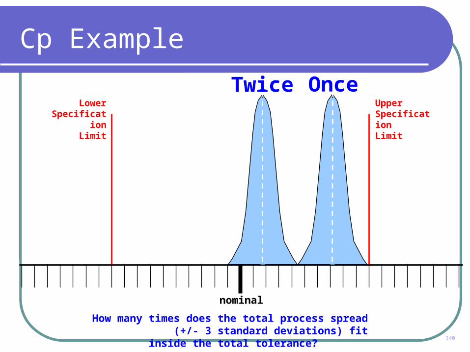
Cp Example
OnceTwice
How many times does the total process spread (+/- 3 standard deviations) fit inside the total tolerance?

141
nominal
UpperSpecificationLimit
LowerSpecificati
onLimit
Cp Example
How many times does the total process spread (+/- 3 standard deviations) fit inside the total tolerance?
OnceTwice3 times

142
nominal
UpperSpecificationLimit
LowerSpecificati
onLimit
Cp Example
OnceTwice3 timesAnd 0.7
How many times does the total process spread (+/- 3 standard deviations) fit inside the total tolerance?
143
nominal
UpperSpecificationLimit
LowerSpecificati
onLimit
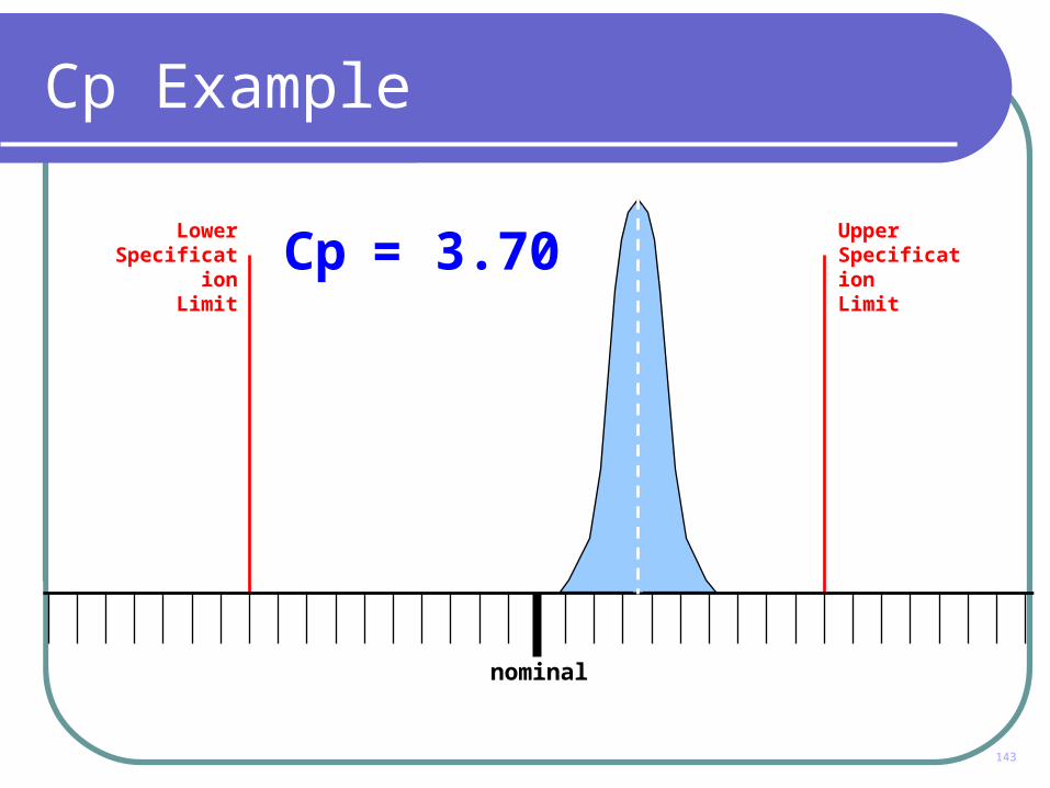
Cp Example
Cp = 3.70

144
nominal
UpperSpecificationLimit
LowerSpecificati
onLimit
Cpk Lower Example
Once
How many times does half the total process spread (3 standard deviations) fit between the mean and the lower specification limit?

145
nominal
UpperSpecificationLimit
LowerSpecificati
onLimit
Cpk Lower Example
Twice
How many times does half the total process spread (3 standard deviations) fit between the mean and the lower specification limit?

146
nominal
UpperSpecificationLimit
LowerSpecificati
onLimit
Cpk Lower Example
3 Times
How many times does half the total process spread (3 standard deviations) fit between the mean and the lower specification limit?

147
nominal
UpperSpecificationLimit
LowerSpecificati
onLimit
Cpk Lower Example
4 Times
How many times does half the total process spread (3 standard deviations) fit between the mean and the lower specification limit?

148
nominal
UpperSpecificationLimit
LowerSpecificati
onLimit
Cpk Lower Example
5 Times
How many times does half the total process spread (3 standard deviations) fit between the mean and the lower specification limit?

149
nominal
UpperSpecificationLimit
LowerSpecificati
onLimit
Cpk Lower Example
Cp = 3.70Cpkl = 5.00

150
nominal
UpperSpecificationLimit
LowerSpecificati
onLimit
Cpk Upper Example
How many times does half the total process spread (3 standard deviations) fit between the mean and the upper specification limit?
Once

151
nominal
UpperSpecificationLimit
LowerSpecificati
onLimit
Cpk Upper Example
Twice
How many times does half the total process spread (3 standard deviations) fit between the mean and the upper specification limit?

152
nominal
UpperSpecificationLimit
LowerSpecificati
onLimit
Cpk Upper Example
And 0.4
How many times does half the total process spread (3 standard deviations) fit between the mean and the upper specification limit?

153
nominal
UpperSpecificationLimit
LowerSpecificati
onLimit
Cp / Cpk Indices
Cp = 3.70Cpku = 2.4

154
Manually calculate Cp / Cpk
Group Exercise
Cpk U = U.S.L. - Process Average
3 x SD
Cpk L =
3 x SD
Process Average - L.S.L.
Cp = Tolerance
6 x SD
• USL = 12• LSL = 8• Mean = 10.5• SD = 0.33

155
Draw Process Capability
Use pencil & paper to draw the following distribution.
Mean = 10.5LSL = 8 USL =12
1 Standard Deviation = 0.33
8 109 11 12 137

156
#1 #2
#3 #4
Relate Cp / Cpk to Archers Target

157
Normal Capability Analysis in Minitab
Stat / Quality Tools / Normal Capability Analysis
Select Stat / Quality Tools /
Capability Analysis /
Normal
Remember! It is imperative that stability and normality tests are conducted before calculating Cpk / Ppk indices.

158
Normal Capability Analysis in Minitab
Stat / Quality Tools / Capability Analysis / Normal
Select Column to
assess
Enter subgroup
size
Enter upper & lower spec.
limits
Click OK

159
12.011.410.810.29.69.08.4
LSL USL
LSL 8Target *USL 12Sample Mean 10.0137Sample N 50StDev(Within) 0.331209StDev(Overall) 0.322772
Process Data
Cp 2.01CPL 2.03CPU 2.00Cpk 2.00
Pp 2.07PPL 2.08PPU 2.05Ppk 2.05Cpm *
Overall Capability
Potential (Within) Capability
PPM < LSL 0.00PPM > USL 0.00PPM Total 0.00
Observed PerformancePPM < LSL 0.00PPM > USL 0.00PPM Total 0.00
Exp. Within PerformancePPM < LSL 0.00PPM > USL 0.00PPM Total 0.00
Exp. Overall Performance
WithinOverall
Process Capability of Tool 1
Normal Capability Analysis in Minitab
Stat / Quality Tools / Capability Analysis / Normal
Short Term Capability
Long Term Capability
For a process to be deemed ‘capable’, the Cpk must be >= 1.67 & the Ppk >= 1.33.

160
For example:
Cpk of 1 = Sigma value of 3
Cpk of 0.5 = Sigma value of 1.5
By converting DPMO and Cpk to a Sigma value we can compare performance between attribute and variable processes.
The higher the Sigma value, the better the process.
To convert Cpk to Sigma we merely multiply the Cpk value by 3 to get the Sigma value.
Cpk conversion to Sigma

161
}Sigma is a universal measure of process performance.
Advantage of using Sigma
VARIABLE DATA
Cp
Pp Ppk
Cpk
ATTRIBUTE DATA DPMODPUDPO

Hypothesis Testing
‘Statistics is never having to say you are right’

163
Hypothesis Testing
Hypothesis Testing Overview
Hypothesis Testing - Proportions
Hypothesis Testing – Variances
Hypothesis Testing - Means

164
Hypothesis Testing Overview
Provides objective solutions to questions which are traditionally answered subjectively.
Can be used to determine a difference in proportions, means and variances (standard deviation).
Graphical analysis indicates a potential difference. Hypothesis testing infers a statistically significant difference
(with a degree of confidence).
A hypothesis test should always be conducted in the improve phase to validate the improvements to the baseline process capability.

165
Variable orAttribute Data?
1 or 2 Factor?
1 or >1 Levels?
Contingency Table
HO : FA Independent FBHA : FA Dependent FB
Stat>Tables>Chi2 Test
Attribute2
Factor
1 Factor
2-Proportion Test
Stat>Basic Stat>2-Proportion
2 Samples2 levels to test for
each 2 levels
1-Proportion Test
Stat>Basic Stat>1-Proportion
1 Sample1 levelto test
Is data normal?
1, 2 or >2levels?
Test formean or sigma?
1-Sample t Test
Stat>Basic Stat>1-Sample t
Chi2 Test
Stat>BasicStat>Display Desc>Graphical Summary(if target sigma falls
between CI, then fail toreject HO )
F Test
Stat>ANOVA>Homogeneity of
Variance
2-Sample t Test
Stat>Basic Stat>2-Sample t
(if sigmas are equal, usepooled std dev to compare.
If sigmas are unequalcompare means using
unpooled std dev)
1 level
2 levels
Test formeans
Test forsigmas
Bartlett's Test
Stat>ANOVA>Homogeneity of VarianceIf sigmas are NOT equal, proceed with caution or use
Welch's Test, which is not available in M initab
More than2 levels
1-Way ANOVA(assumes equality of
variances)
Stat>ANOVA>1-Way(then select stacked or
unstacked data)
Test for means
Data Normal
HO: 1 = t
HA: 1 t
t = target
Levene's Test
Stat>ANOVA>Homogeneity of Variance
If HO is rejected, then you cango no further
Datanot
Normal
1, 2 or morelevels?
Test medianor sigma?
1 level
Chi2 Test
Stat>BasicStat>Display Desc>Graphical Summary(if target sigma falls
between CI, then fail toreject HO )
HO: 1 = t
HA: 1 t
t = target
Test for sigmas
1-Sample Wilcoxon or1-Sample Sign
Stat>Non-parametric>and either 1-Sample
Sign or 1-SampleWilcoxon
TestMedians
2 ormorelevels
M ann-Whitney Test
Stat>Non-parametric>M ann-Whitney
M ood's M edian Test(used with outliers)
Stat>Non-parametric>M ood's test
Kruskal-Wallis Test(assumes outliers)
Stat>Non-parametric>Kruskal-Wallis
2 ormorelevels
HO: M1 = M2
= M3 ...
HA: M i Mj for i j
(or at least one is different)
HO: M1 = M2
= M3 ...
HA: Mi Mj for i j
(or at least one is different)
HO: M1 = Mt
HA: M1 Mt
t = target
HO: M1 = M2
HA: M1 M2
H O : 1 = 2
= 3 ...
H A : i j for i j
(o r a t least one is d iffe ren t)
HO: 1 = t
HA: 1 t
t = target
HO: 1 = 2
= 3 ...
HA: i j for i j
(or at least one is different)
HO: 1 = 2
HA: 1 2
HO: 1 = 2
= 3 ...
HA: i j for i j
(or at least one is different)
HO: P1 = Pt
HA: P1 Pt
t = target
HO: P1 = P2
HA: P1 P2
2 levels only
If P > 0.05, then fail to reject H O If P < 0.05, then reject H O Ensure the correct sam ple size is taken.
1, 2 or moreFactors?
Variable
2 levels or> 2 levels?
Fail to reject H O
Courtesy of Jeff Railton and Andy Battyof Seagate Technology.Revised: June 23, 1999
(Hypothesis Roadmap E.vsd)
ST ART >>>
2 or more Factors
1Factor
HO : Data is normalHA : Data is not normal
Stat>Basic Stat>Normality Test orStat>Basic Stat>Descriptive Statistics
(graphical summary)
HO: 1 = 2
HA: 1 2
ANOVA orMultiple Regression
Is DataDependent?
No,Data is drawnindependently
from twopopulations
Paired t Test
Stat>Basic Stat>Paired t
HO: 1 = 2
HA: 1 2
Yes,Data isPaired
Test formean or sigma?
Test forsigmas
Test formeans
Hypothesis Testing Roadmap

166
Hypothesis Testing – Proportions
Stat / Basic Statistics / 2 Proportions
Stat / Basic Statistics / 2 Proportions
Enter trials (sample size) & events (defects)
in the option box
Click OK

167
Hypothesis Testing – Proportions
Stat / Basic Statistics / 2 Proportions
P-Value < 0.05 indicates a significant difference
Either accept, or fail to accept the null hypothesis. It is assumed there is no difference unless proven otherwise. I.e. Innocent until proven guilty!

168
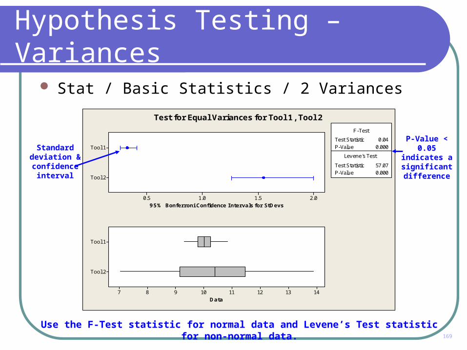
Hypothesis Testing – Variances
Stat / Basic Statistics / 2 Variances
Stat / Basic Statistics / 2 Variances
Always conduct a normality test before conducting a hypothesis test on variable data.
Enter variables to
compare
Click OK
169
Hypothesis Testing – Variances
Stat / Basic Statistics / 2 Variances
Standard deviation & confidence
interval
95% Bonferroni Confidence Intervals for StDevs
Tool 2
Tool 1
2.01.51.00.5
Data
Tool 2
Tool 1
1413121110987
Test Statistic 0.04P-Value 0.000
Test Statistic 57.07P-Value 0.000
F-Test
Levene's Test
Test for Equal Variances for Tool 1, Tool 2
P-Value < 0.05 indicates a significant difference
Use the F-Test statistic for normal data and Levene’s Test statistic for non-normal data.

170
Hypothesis Testing – Means
Stat / Basic Statistics / 2 Sample t
Stat / Basic Statistics /
2 Sample t
Always conduct a normality and 2 variances test before conducting a 2 Sample T test. However, if the sample sizes are equal, the requirement to conduct a 2 variances test is not applicable.
Enter variables to
compare
Select equal variances if applicable
Click OK
Select boxplot

171
Hypothesis Testing – Means
Stat / Basic Statistics / 2 Sample t
P-Value >= 0.05 infers that the
means are from the same
population
If the P is low, the null must go!

172
Summary
What is Six Sigma? Introduction to Minitab Version 14 Manipulation of data Basic statistics Graphs Quality tools Measurement System Analysis – R & R Control charts Normality testing Capability analysis Hypothesis Testing

173
Questions and Answers
Created by Paul White - Aston Martin Six Sigma DepartmentSources:Ford Six Sigma Black Belt Training Material 2006Ford Six Sigma Green Belt Training Material Version 5.0Jaguar SPC Training Material 2004