milne’s differential equation and numerical solutions...

J. Phys. B: At. Mol. Phys. 15 (1982) 1-15. Printed in Great Britain

Milne’s differential equation and numerical solutions of the Schrodinger equation 11. Complex energy resonance states

H J Korsch, H Laurent and R Mohlenkamp Fachbereich Physik, Universitat Kaiserslautern, D-6750 Kaiserslautern, West Germany

Received 2 July 1981, in final form 27 August 1981

Abstract. The combination of Milne’s theory for calculating bound-state energies and wavefunctions with the complex rotation method yields an appealingly simple and powerful tool for the computation of complex-valued resonance (Siegert) energies and wavefunctions. The method provides an unambiguous assignment of a quantum number n = 0, 1, , . . to a resonance state and permits a unified picture of bound-state and resonance properties. The numerical technique is sufficiently fast and stable to enable reliable calculations of higher resonances. This is illustrated for some model potentials. Furthermore the complex energy WKB quantisation is discussed and tested numerically.

1. Introduction

In a previous paper (Korsch and Laurent 1981), hereafter denoted as I, we rein- vestigated the Milne (1930) method for calculating bound-state energies and wavefunctions. It was found that the Milne theory provides a very appealing and powerful numerical technique which was superior to other methods, especially for higher quantum numbers. In the present article we extend the theory developed in I to the case of complex-valued resonance or Siegert states (Siegert 1939), i.e. solutions of the radial Schrodinger equation

with boundary conditions

U l ( 0 ) = 0 (2)

ul ( r ) - eikr (3)

and

with wavenumber k = (2mE)1’2/h. For simplicity we drop the orbital wavenumber 1 from all quantities in the following. All of the sample calculations presented in 0 4 are carried out for 1 = 0.

The completely outgoing behaviour can only be achieved for complex values of k = ko-ikl (note that kl 2 0, so that u ( r ) is not square integrable), i.e. complex energies

E = ER -$I- (4)

0022-3700/82/010001+ 15$02.00 @ 1982 The Institute of Physics 1

2 H J Korsch, H Laurent and R Mohlenkamp

where ER and r(r > 0) are the resonance position and width. The complex-valued energies singled out by the boundary conditions (2) and (3) can also be described as poles of the S matrix.

For very narrow isolated resonances close to the real axis the position E R and the width r defined in this way agree with other definitions using only real energies. The most popular alternative description of a resonance is undoubtedly the step-like behaviour of the scattering phaseshift v ( E ) , where the resonance is defined by the position of the maximum of the collisional time delay function (see, for example, LeRoy and Liu 1978)

877 T(E) = 2ti-

8 E

i.e. we have &/8E = 0 at E R and the width is defined by the maximum time delay (the lifetime of the metastable state) as

r = ~ ~ / T ( E R ) . (6)

It is worthwhile, however, pointing out that the relationship between both approaches is not one to one (even for sharp resonances). It has been shown for certain potentials that the phaseshift may possess a sharp, isolated Breit-Wigner-type resonance, without an S-matrix pole associated with it. The reverse situation may also be noted: a complex pole of the S matrix does not necessarily induce a resonance-like structure in the phaseshift (see, for example, the review article by Fonda et a1 1978 and the references given there). Normally, however, a direct correspondence between the complex energy pole and the phaseshift characterisation of resonances is observed, with good numerical agreement for sharp resonances. For broad resonances, however, in the vicinity or above the potential maximum marked discrepancies have been found (Hehenberger et a1 1976a, b, Hehenberger 1977, LeRoy and Liu 1978, Atabek et a1 1980).

In the following we concentrate on complex energy resonances. Various theoretical and numerical methods have been used for the computation of these states. We would like to mention the Weyl-Titchmarsh function (Hehenberger et a1 1976a, b, Hehen- berger 1977), the (variational) basis set expansion method which includes non-square- integrable functions (Bardsley and Junker 1972, Isaacson et a1 1978) and the direct numerical inward integration of the Schrodinger equation (Clayton and Derrick 1977).

In an increasing number of applications the complex rotation method is used (see, for example, Atabek et a1 1980, Bain et a1 1974, Bardsley and Junker 1972, Clayton and Derrick 1977, Doolen 1975, Doolen et a1 1974, 1978, Gazdy 1976, 1980, Moiseyev et a1 1978, Morgan and Simon 1981, Winkler 1977, Yaris et a1 1978, and in particular the special issue of the Int. J. Quant. Chem. 14 (6) (1978)). The complex rotation r = p eis transforms the Schrodinger equation (1) into

witht & = e2ieE and e ( p ) = ezie V ( p e"). u"(p) = u ( p eie) is, however, asymptotically decaying provided that the rotation angle satisfies

8 >tan-' k l f ko. (8)

t Here and in the following we use the tilde'" to denote &dependent complex rotated quantities.

Milne’s differential equation 3

This method obviously requires that the potential V can be analytically continued into the complex plane; more precisely, the complex rotation method has been proved mathematically to be correct for dilatation analytic potentials (see e.g. Aguilar and Combes 1971, Balslev and Combes 1971, Simon 1972).

The great advantage of the complex rotation method is the simple fact that the resonance solutions of (7) are square integrable so that (7) can be solved for the eigenvalue by bound-state techniques.

The wavefunction can be expanded in (square-integrable) basis functions and the Ritz-Raleigh variational principle gives the resonance energies as complex eigenvalues of a non-Hermitian Hamiltonian matrix (see, for example, Moiseyev et a1 1978, Atabek et a1 1980 and references therein). In this approximation (the basis set is necessarily finite) the resonance energy shows a typical dependence on the rotation angle 8 (called the 8 trajectory) and special techniques have been developed to locate the best estimate of the eigenvalue from the loops, bends and kinks of these trajectories. An alternative is the direct (inward) integration of (7) as used by Clayton and Derrick (1977) or the recent adaptation of the popular Cooley technique for the determination of real energy bound states (see I) to the complex energy resonance case, which has recently been developed and investigated by Atabek et a1 (1980).

The present work suggests a different direct approach via Milne’s non-linear differential equation, which is also an extension of a real energy bound-state method discussed in detail in I. In the following section Milne’s quantisation condition is extended to the complex energy case. In Q 3 an approximate semiclassical quantisation is discussed and Q 4 presents numerical results for model potentials. The paper concludes with a short discussion.

2. Milne’s complex energy quantisation condition

Milne’s method for the solution of real energy bound-state problems (i.e. Hermitian Hamiltonians) has been discussed in detail in I. The method can be directly extended to the non-Hermitian case (7): the solution G ( p ) of (7) is written as

C ( p ) = c C ; ( p ) sin K 2 ( p ’ ) dp’. I (9)

c is a normalisation constant and $ ( p ) is an arbitrary solution of Milne’s non-linear differential equation

with

w2 2m - l(1-t 1) k ( p ) = + E - F ( p ) ) - -

h P 2

The requirement of an asymptotically ( p + 00) decaying wavefunction (provided that the condition (8) for the complex rotation angle 8 is satisfied) leads to the condition

N ( E N ) = n + 1 n = 0 , 1 , . . . (12)


where-as in I-the quantum-number function

and the quantum momentum

have been introduced. The solution of the quantisation condition (12) determines the complex resonance energies E,. All resonances are located on the curve defined by Im N ( E ) = 0. Furthermore, equation (12) assigns unambiguously a quantum number n to each complex energy resonance state, which agrees with the usual quantum number (compare I) if the potential possesses real energy bound-states below the continuum threshold. Previously such an assignment of a quantum number for a resonance state could only be given by inspecting the wandering of the resonance poles in the complex plane if the potential is made more and more attractive until the state under inspection develops into a true bound state at real energy with the desired quantum number (see, for example, the study of the square-well potential by Nussenzveig 1959). In the case of resonance studies at real energies via the phaseshift methods the quantum number is usually, by means of heuristic arguments, related to the number of nodes of the wavefunction until the outermost classical turning point is reached; a concept which is obviously quite useful for sharp resonances below the potential maximum.

The quantum momentum k ( p ) decays to zero asymptotically, and the integral (12) is independent of the complex rotation angle 8, provided that the quantum momentum k(p) is an analytic function in the complex plane. This is not the case, however, because in contrast to the real energy case discussed in I the Milne function 5 may possess zeros in the complex plane, i.e. k(p) can have a pole. In this case the quantum number function picks up a contribution from the pole when the complex rotation angle becomes larger than the phase angle of the pole.

The contribution of a pole at ro = po exp(iOo) can be found quite easily: let us assume that po is a zero of i ’ j of order v, i.e. 6 = [ ( p -p0 ) /d ] ’ . Inserting this ansatz into Milne’s differential equation (10) we find that the only possibility of satisfying (10) is v = 1 (i.e. k has a first-order pole at ro) and d = *ii. Integrating k( p ) over the contour C shown in figure 1, which is closed at infinity, we find by means of the residuum theorem

and we have

N ( E I el) = N ( E 1 e2)* 1.

It is clear, that the solution of the quantisation condition (12) cannot lead to a wrong resonance energy, but only to a wrong assignment of the quantum number. If there is any doubt about the correctness of the assignment, it can easily be checked by repeating the calculation with different rotation angles.

Closing this section we would like to note that a closed-form expression for the density of states dN/dE can be derived, which is simply the complex continuation of the result given in I. The reader is therefore referred to this work.


qgure 1. Complex r-plane illustrating the influence of a pole of the quantum momentum K ( r ) at ro (0) on the quantum number function N ( E ) .

3. Semiclassical complex energy quantisation

In a numerical application of the Milne method for the calculation of complex energy resonances (details are given in § 4) it is often useful to have an initial estimate of the resonance energy E,. Such an approximate value can for example be provided by WKB

methods. The semiclassical limit (ti -+ 0) of the complex energy resonance states has been

discussed by various authors (see, for example, the reviews by Child 1974 and Connor 1976, 1980 and the original papers by Connor 1968, 1972, 1973, Dickinson 1970 and Drukarev et a1 1979). The complex energy semiclassical quantum number function is given by Connor (1968, 1972, 1973)

( ~ ) = r - ’ { a -t~[1-ln(-~)]+3i[31n2.rr+t.rrs - 1 n r ( t - i ~ ) ] ) + 3 (16) NWKB

for effective potentials with a minimum and a barrier (on the real r axis) where 1 r r 2

a ( E ) = I J p( r ,E )d r ti r l

is the action integral over the potential well and

is the action integral over the barrier. 1 2 2 p ( r ,E )=[2m(E- V(r))-(l+T) h /r2]1’2

is the classical momentum (the celebrated Langer transformation 1 ( I + 1) -+ (I + t)’ has been used). For complex energies, rl, r2 and r3 denote the complex continuation of the ordered (rl < r2 < r3 ) turning points for real energies between the minimum and the maximum of the potential. The WKB resonance energies E:KB are given by the solution of

NWKB(EFKB) = n + 1. (19)


It should be noted that in the limit of very broad barriers (or deep potentials) le 1 + 00

equations (16) and (19) reduce to the usual WKB quantisation formula

1 r2 - p(r, E) dr = h(n ++). T I,,

In the opposite extreme of high quantum numbers equation (16) reduces to the two-point formula

1 r3 - p(r, E ) dr = h(n +t ) . I, These limiting forms of equation (16) are well known in connection with Regge

poles (Delos and Carlson 1975, Connor et a1 1976, Thylwe 1981), but they have apparently never been discussed for complex-valued energies.

Numerically equation (19) can be solved by means of a complex Newton method starting from an initial guess (which may be rather crude) and using the WKB density of states

with T ( z ) = d/dz In T(z) and

aa m r2 dr aE - h I,, a& im r 3 dr aE I T ~ / ~ , P(r,* _- - --

It is surprising that the quality of the complex energy WKB quantisation formula (16) has never been investigated numerically:.

A test calculation by the authors (Korsch et a1 1981) showed good agreement with exact quantum results. Further, and more extensive, numerical comparisons are given in the following section. It should be noted that the semiclassical results can be substantially improved by means of higher-order phase integral methods (Froman and Froman 1965, 1974a, b, 1978).

4. Numerical applications

As an illustrative example of the method for the numerical evaluation of complex resonance energies by means of the method described in § 2 we first consider the model potential

~ ( r ) = Vor2 ePhr ( 2 5 )

which has a barrier of height VB = 4 Vo e-’/h2 at rB = 2 / h . Here and in the following we use units with h = 1 and m = 1; we furthermore restrict ourselves to s waves. For the

f The same semiclassical quantisation formula (16) is, however, also valid in the real energy/complex angular momentum case, i.e. for Regge poles. In this case, various numerical applications have been published (Connor eta1 1976,1979,1980, Connor and Jakubetz 1978, Delos and Carlson 1975, Sukumar and Bardsley 1975).

Milne's differential equation 7

- 0 5 -

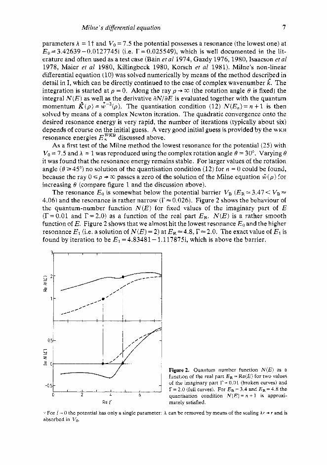
parameters A = 1 t and Vo = 7.5 the potential possesses a resonance (the lowest one) at E, = 3.42639 - 0.01277453 (i.e. r = 0.025549), which is well documented in the literature and often used as a test case (Bain et a1 1974, Gazdy 1976,1980, Isaacson et al 1978, Maier et a1 1980, Killingbeck 1980, Korsch et a1 1981). Milne's non-linear differential equation (10) was solved numerically by means of the method described in detail in I, which can be directly continued to the case of complex wavenumber k: The integration is started at p = 0. Along the ray p +CC (the rotation angle 8 is fixed) the integral N ( E ) as well as the derivative aN/aE is evaluated together with the quantum momentum k ( p ) = G- ' (p ) . The quantisation condition (12) N(E,) = n + 1 is then solved by means of a complex Newton iteration. The quadratic convergence onto the desired resonance energy is very rapid, the number of iterations (typically about six) depends of course on the initial guess. A very good initial guess is provided by the WKB

resonance energies EYKB discussed above. As a first test of the Milne method the lowest resonance for the potential (25) with

V, = 7.5 and A = 1 was reproduced using the complex rotation angle 6 = 30". Varying 8 it was found that the resonance energy remains stable. For larger values of the rotation angle (8 a45") no solution of the quantisation condition (12) for n = 0 could be found, because the ray 0 s p + 00 passes a zero of the solution of the Milne equation G ( p ) for increasing 8 (compare figure 1 and the discussion above).

The resonance Eo is somewhat below the potential barrier VB (ER = 3.47 < VB = 4.06) and the resonance is rather narrow (r = 0.026). Figure 2 shows the behaviour of the quantum-number function N ( E ) for fixed values of the imaginary part of E (r = 0.01 and r = 2.0) as a function of the real part ER. N ( E ) is a rather smooth function of E. Figure 2 shows that we almost hit the lowest resonance Eo and the higher resonance El (i.e. a solution of N ( E ) = 2) at ER = 4.8, r = 2.0. The exact value of El is found by iteration to be El = 4.83481 - 1.117875, which is above the barrier.

- of the imaginary part r = 0.01 (broken curves) and I I I I I I , . r = 2.0 (full curves). For E R = 3.4 and E R = 4.8 the


Calculations of higher resonances are surprisingly rare in the literature; as an example of such calculations we would like to note the classic paper by Nussenzveig (1959) on the square-well potential, which discusses the behaviour of the poles of the S matrix in the complex k plane for varying potential depth. Hehenberger et a1 (1976) discuss two close resonances for the HgH potential for the rotational quantum state I = 9. The only study of a longer series of resonances for an analytic potential, at least to our knowledge, can be found in an article by Yaris e? al (1978) for the potential $x’ -Ax3(A > 0 , -CO < x < CO). This potential has, however, a different character (it is not a radial problem and V ( x ) + CO for x + CO) than the potentials investigated in the present study so that we did not try a comparison.

Because of this situation we find it useful to present some more extensive numerical results for the model potential (25). Table 1 gives a number of complex energy

Table 1. Exact and WKB complex resonance energies E, = E,(n) - $ r ( n ) ( n = 0, 1, . . .) for the model potential (25) ( m = h = A = 1) for various potentials Vo, i.e. various barrier heights V,. For convenience the complex wavenumber k , and the rotation angle 6, for which the resonance was safely found, are also listed. The WKB resonance energies marked by a dagger are calculated by means of the two turning point formula (21).

8 V, V, n (deg) k ( n ) k , ( n ) ER(n) r ( n ) EzKB(n) rwKe(n)

3.75 2.030 0 30 1 44 2 44 3 45 4 60 5 60

7.5 4.060 0 30 1 30 2 30 3 44 4 44 5 50 6 55 7 57.5

15 8.120 0 30 1 30 2 30 3 44 4 44 5 44 6 45 7 50 8 55 9 57.5

10 60

22.5 12.180 0 30 1 30 2 30 3 30 4 44 5 44 6 45 7 45 8 50 9 50

2.01860 2.35653 2.55465 2.68929 2.78607 2.85597

2.61779 3.13004 3.39839 3.59146 3.73831 3.85346 3.94486 4.01737

3.30522 4.17941 4.51381 4.77594 4.98315 5.15204 5.29255 5.41092 5.51131 5.59661 5.66900

3.75267 4.93115 5.32910 5.63772 5.88577 6.09116 6.26480 6.41376 6.54219 6.65527

-4.86258-2 -0.577984 -1.24117 -1.90698 -2.56018 -3.19776

-4.87989-3 -3.57144- 1 -9.97252 - 1 -1.66396 -2.33178 -2.99225 -3.64246 -4.28166

- 1.76028-5 -1.28102- 1 -6.77880 -- 1 -1.31977 -1.9841 1 -2.65326 -3.32019 -3.98165 -4.63615 -5.28304 -5.92211

-7.94048-8 -3.61526 - 2 -4.61961 - 1 - 1.07058 -1.72050 -2.38537 -3.05444 -3.72258 -4.38708 -5.04650

2.03620 2.60959 2.49286 1.79786 6.03838 - 1

-1.03457

3.42639 4.83481 5.27728 5.06493 4.26886 2.94778 1.14718

-1,09669

5.46224 8.72552 9.95749 1.05339+1 1.04475+ 1 9.75187 8.49374 6.71227 4.44031 1.70575

- 1.46690

7.04126 1.21575+ 1 1.4092911 1 . 5 3 1 8 9 ~ 1 1.58411+1 1.57061 + 1 1.49591 + 1 1 . 3 6 3 9 4 ~ 1 1.17808+ 1 9.41270

1.96312-1 2.72408 6.34151 1.02569+ 1 1,42657 + 1 1.82654+1

2.55490-2 2.23575 6.77810 1.19521 + 1 1.74338+ 1 2.30610+1 2.87380t 1 3.44020 + 1

1.16362 -4 1.07078 6.11965

1.97742 + 1 2.73394+ 1 3.51445+ 1

5.1 1025 + 1 5.91343 + 1 6.7144811

1.26063 + 1

4.30888 + 1

0.59594-6 3.56548 - 1 4.92367

2.02529 + 1 2.90594.t 1 3.82710+ 1 4.77514+1 5.74075 + 1

!.20713+ 1

6.71717+ 1

2.092 2.055 - 1 2.648 2.743 2.522 6.359 1.819: 1 .027+lt 6.227-lt 1.428+1t

3.497 2.787-2 4.880 2.260 5.315 6.799 5.096 1.197+1 4.296 1.745+1 2.969t 2.307+1t 1.166t 2.875+1t

5.552 1.321-4 8.778 1.089

1.057+1 1.263+1 1.048+1 1.979+1 9.783 2.736+ 1 8.522 3.516+1 6.735: 4 . 3 1 0 t l ~ 4.461t 5 .111+lt 1.725: 5.915+1:

1.000+1 6.145

7.144 0.684 - 6 1.2221 1 3.661 - 1 1.414+1 4.951 1.536+1 1.210+1 1.588+1 2.028+1 1.574+1 2.908+1 1.499+1 3.829+1 1.367+1 4.777+1 1.181+1 5.742+1


resonances E,, for various potential strengths Vo. It is interesting to note that the real part of E,, increases with n for low n, reaches a maximum and decreases again for higher resonances. We are not aware of an observation of such a behaviour of the resonance positions for other potentials. The resonance wavenumbers k,, however, show the expected behaviour, i.e. the real part of k , is monotonically increasing with n. The results, particularly those with negative ER, are unusual and their interpretation is not yet clear. The general behaviour of the pole string in the complex E plane is currently under investigation and the discussion will be deferred to a future publication. Figure 3 shows the positions of the resonances in the complex k plane for various values of Vo. All resonances are constrained to lie on the curves Im N ( E ) = 0, which are also shown in figure 3. With increasing potential strength Vo, i.e. with increasing barrier height VB, the position of the resonances (i.e. the real part ER) increases and the width decreases.

Re k

Figure 3, Positions of the resonances E,, n = 0, 1, . . . in the complex wavenumber plane for the model potential ( 2 5 ) with various potential strengths V,, = 3.75, 7.5, 15 and 22.5. The resonances lie on smooth curves, on which the imaginary part of the quantum number function (13) vanishes.

Table 1 furthermore lists the values of the rotation angle 13, for which the resonance E, was safely detected. For considerably higher or lower values the resonances could not be found for this value of n, because of the sudden jumps of the N ( E ) function at the critical angles (compare the discussion above in context with figure 1).

For comparison the complex WKB resonance energies obtained by solving equation (19) are also listed in table 1. The values marked by daggers are determined by means of equation (21). Numerically the quantisation equations (19) or (21) are solved by Newton iteration using equations (22)-(24). The phase integrals (17), (18) and their derivatives (23), (24) are evaluated by a complex extension of the standard Gauss- Mehler method integrating along a straight line between the turning points.

The integration is sufficiently fast for low quantum states. For higher quantum numbers, however, we encountered numerical difficulties. The complex momentum develops a rather sharp extremum along the integration path so that a large number of integration points were needed to evaluate the phase integrals (17) and (18) with the required accuracy. This difficulty could not be overcome using the Clenshaw-Curtis integration method (Kennedy and Smith 1967, Connor and Jakubetz 1978) instead of

10 . H J Korsch, H Laurent and R Mohlenkamp

the Gauss-Mehler procedure. In this high quantum number region the simplified two turning point formula (21) was found to be in good agreement with the three turning point results (16), where no such difficulties were observed for energies with positive real part. For even higher states with negative real part of the resonance energy no converged semiclassical results could be obtained. The reason for this behaviour is not yet clear.

The agreement between the exact complex resonances and the WKB approximation is surprisingly good. This is especially worthwhile to note for the broad and very broad resonances close to and above the potential threshold where other (real energy) WKB

techniques showed marked discrepancies (see, for example, Le Roy and Liu 1978 and Connor and Smith 1981).

Figure 4 shows the wavefunctions & ( p ) for the lowest resonances of the potential (25) (A = 1, Vo = 7.5) along the ray 0 s p < CO in the complex U', plane (similar plots have been obtained by Atabek et a1 (1980) for a different potential). The wavefunctions show a complicated behaviour: they start at Li, = 0 for p = 0, perform various spirals around the origin-with occasional reversals of the direction of rotation-and end again at U', = 0 for p + 00. In contrast to the bound-state case we could not find a simple

n = b

Re

Figure 4. Wavefunctions U',(p) (arbitrary units) for the potential ( 2 5 ) (A = 1, V, = 7 . 5 ) in the complex U plane (i.e. imaginary part of U', plotted against real part for 0 < p <CO). The lowest eight ( n = 0, 1, . . . , 7 ) resonance states are shown. The corresponding complex rotation angles are listed in table 1.


n = O

n= 2

rule to find the quantum number n directly from the wavefunction. The oscillatory behaviour is certainly increasing with n, and so are the number of crossings with an axis through the origin (say the imaginary axis). However, such an assignment can easily be misleading. Figure 5 shows ICn(p)l2 as a function of p. We clearly see the square- integrable character of the wavefunctions: they decrease rapidly for larger values of p. Here we observe a direct correspondence between the number of minima and the quantum number n. A similar behaviour has been found for the potential V ( x ) = $ x 2 - h x 3 by Yaris er a1 (1978) for the lowest resonances ( n = 0, 1,2).

n = l

~

I n.3 i I

- n = L

9 Figure 5. Absolute square of the wavefunctions shown in figure 4 as a function of p .

n = 5 i

The oscillatory behaviour of l&(p)12 depends, however, on the rotational angle e. For larger values of 8 the oscillations are quenched, so that an assignment of the quantum number n by counting the minima of 1L;,(p)12 is no longer possible. Figure 6 demonstrates this for the state n = 6; if the complex rotation angle e is increased from 8 = 55" (as in figures 4, 5 ) to 8 = 60°, the oscillations of lU",(p)l' have almost disap- peared.

Figure 7 finally gives an impression of the behaviour of the quantum momentum k ( p ) = K 2 ( p ) (equation (14)), i.e. of the solution of the Milne equation (10). k ( p ) starts at p = 0 at a point in the complex k plane, which is prescribed by the classical initial condition for the solution of (10) (compare I) and decreases to zero for p +CO. In the complex k plane we see some typical loops and kinks, which give rise to oscillations of lk12. Figure 7 also demonstrates the influence of thezeros of 6 ( p ) , i.e. poles of k ( p ) : for the resonance state n = 4 we almost hit such a zero, which manifests itself as a sharp


Figure6. Wavefunction C n ( p ) in the complex U

plane (upper panel) and I l i , (p)i2 (lower pane1)for the potential ( 2 5 ) (same parameters as in figures 4 and 5 ) for a larger value of the complex rotation angle 0 = 60". Note that the oscillations of lC,(p)i2 shown in figure 5 are almost completely quenched.

P

Figure7. Quantum wavenumber Z ( p ) for the potential ( 2 5 ) ( A = 1, V,,=7.5) and the resonance states n = 3 and n = 4 (same rotation angles 0 as in table 1).

spike in \g(p)lz at p ~ 4 . 6 . In such a case, of course, the integration of the quantum actior, integral (13) is problematic and shows up a numerical instability in the N ( E ) function. It is therefore preferable to avoid this problem by choosing a different rotation angle 8.


As a second example for an application of the Milne method we consider the one-dimensional (-CO < r < +CO) potential

V(r) = ($r2-J) exp(-Ar2)+J (26) studied by Moiseyev er a1 (1978), Atabek et a1 (1980) and Killingbeck (1981). Again we use units with h = m = 1. In this one-dimensional case the quantum number function (13) must be replaced by

1 " N ( E ) = - I k ( r ) dr.

77- -" Because of the symmetry of the potential the integration to -CO is replaced by a

duplication of the quantum number function obtained from integration to positive values. Table 2 gives the lowest complex resonance energies E,, = ER(^) -$ir(n) for J=O.8 and A =0.1 (for n = 0 we actually have a bound state). The bound state at Eo = 0.5 has been mentioned by Moiseyev et a1 (1978) and the n = 2 resonance agrees with the value (more precisely the DCRM result) by Atabek et a1 (1980) (ER = 2.12720, r = 0.0308946) and is in reasonable agreement with the approximate value (ER = 2.124, r = 0.037) obtained by Moiseyev er a1 (1978). The sharp n = 1 resonance has apparently not been noticed before. The broad n = 3 resonance is above the barrier V, = 2.367 (i.e. ER> VB), In table 3 we finally compare our results for the n = 2 resonance with those given by Atabek et a1 (1980) for various values of the steepness

Table 2. Complex resonance energies E,, = E R ( n ) - $ r ( n ) f u the potential (26) with J = 0.8 and A = 0.1.

0.502040 1.42097 2.12720 2.58458 2.92442 3.25549 3.55722 3.82433

0 1.16558 -4 3.08946 - 2 3.47501 - 1 1.12959 2.22306 3.51101 4.97489

Table 3. Complex resonance energies E,, = ER-$T for the potential (26) with J = 0.8 and n = 2 for various values of A , i.e. various barrier heights V,.

A VB ER= ra E R b rb

0.08 2.823 2.22476 2.35002 - 3 2.22476 2.35003 - 3 0.09 2.570 2.17749 1.08457-2 2.17749 1.08457-2 0.10 2.367 2.12720 3.08947-2 2.12720 3.08947-2 0.11 2.202 2.07675 6.39994-2 2.07674 6.39994 - 2 0.12 2.065 2.02839 1.08139-1 2.02838 1.08143 - 1 0.13 1.949 - - 1.98318 1.60258-1 0.14 1.850 - - 1.94140 2.17641 - 1

a Atabek et al (1980) (DCRM results). Present work.


parameter A. We find good agreement with their DCRM results, up to small deviations in the last digits of the resonance width r, which may be due to numerical rounding errors. Atabek et a1 somehow stopped their series of A values when the resonance comes close to the barrier, for reasons not known to us. In order to demonstrate the applicability of the method proposed in the present articlein the region above the barrier we continued the A values into this region.

5. Conclusions

The Milne method for calculating bound states has been extended to the case of complex energy resonances. A numerical technique has been developed, which allows fast and reliable computations of resonance energies and wavefunctions; this was demonstrated for two model potentials for both very sharp and very broad resonances.

The exact resonances calculated in this way have been compared with semiclassical (WKB) results. The agreement was very good and no discontinuities or marked deviations could be detected for higher resonances close to the potential barrier or for very broad resonances far away from the real axis.

In future applications we plan to use the methods described in the present article to study more complicated systems, including field ionisation of Rydberg atoms. It has also not escaped the attention of the authors that the Milne method-combined with a complex rotation (Sukumar and Bardsley 1975)-offers an interesting alternative for the exact calculation of Regge poles in the complex I plane.

It would seem interesting to investigate the completeness properties of the resonance states in more detail (compare the recent article by Romo 1980), as well as the direct computation of physically observable (real energy) quantities (as, for example, reflection probabilities or cross sections) via the complex energy pole formalism.

Acknowledgment

The authors are grateful to acknowledge financial support by the Deutsche For- schungsgemeinschaft and helpful correspondence from 0 Atabek and R Lefebvre as well as from P Winkler.

References

Aguilar J and Combes J M 1971 Commun. Math. Phys. 22 269-79 Atabek 0, Lefebvre R and Requena A 1980 Mol. Phys. 40 1107-15 Bain R A, Bardsley J W, Junker B R and Sukumar C V 1974 J. Phys. B: At. Mol. Phys. 7 2189-202 Balslev E and Combes J M 1971 Commun. Math. Phys. 22 280-94 Bardsley J N and Junker B R 1972 J. Phys. A: Math. Gen. 5 L178-80 Child M S 1974 Mol. Spectrosc. 2 466-512 Clayton E and Derrick G H 1977 Aust. J. Phys. 30 15-21 Connor J N L 1968 Mol. Phys. 15 621-31 - 1972 Mol. Phys. 23 717-35 - 1973 Mol. Phys. 25 1469-73 - 1976 Chem. Soc. Rev. 5 125-48 - 1980 Semiclassical Methods in Molecular Scattering and Spectroscopy ed M S Child (Dordrecht: Reidel)

pp 45-107

Milne 's differential equation 15

Connor J N L and Jakubetz W 1978 Mol. Phys. 35 949-64 Connor J N L, Jakubetz W, MacKay D C and Sukumar C V 1980 J. Phys. B: Ai. Mol. Phys. 13 1823-37 Connor J N L, Jakubetz W and Sukumar C V 1976 J. Phys. B: At. Mol. Phys. 9 1783-99 Connor J N L, MacKay D C and Sukumar C V 1979 J. Phys. E: At . Mol. Phys. 12 L515-9 Connor J N L and Smith A D 1981 Mol. Phys. 43 397-414 Delos J B and Carlson C E 1975 Phys. Rev. A 11 210-20 Dickinson A S 1970 Mol. Phys. 18 441-9 Doolen G D 1975 J. Phys. B: Af. Mol. Phys. 525-8 Doolen G D, Nuttall J and Stagat R W 1974 Phys. Rev. A 10 1612-5 Doolen G D, Nuttall J and Wherry C J 1978 Phys. Rev. Lett. 40 313-5 Drukarev G, Froman N and Froman P 0 1979 J. Phys. A : Math. Gen. 12 171-86 Fonda L, Ghirardi G C and Rimini A 1978 Rep. Prog. Phys. 41 587-631 Froman N and Froman P 0 1965 JWKB-Approximation, Contributions to the Theory (Amsterdam: North-

- 1974a Ann. Phys., N Y 83 103-7 - 1974b Nuovo Cim. B 20 121-32 -1978 J. Math. Phys. 19 1830-7 Gazdy B 1976 J. Phys. A: Maih. Gen. 9 L39-41 - 1980 Phys. Lett. 76A 367-8 Hehenberger M 1977 J. Chem. Phys. 67 1710-1 Hehenberger M, Froelich P and Brandas E 1976a J. Chem. Phys. 65 4571-4 Hehenberger M, Laskowski B and Brandas E 1976b J. Chem. Phys. 65 4559-70 Isaacson A D, McCurdy C W and Miller W H 1978 Chem. Phys. 34 311-7 Kennedy M and Smith F J 1967 Mol. Phys. 13 443-8 Killingbeck J 1980 Phys. Lett. 78A 235-6 - 1981 private communication Korsch H J and Laurent H 1981 J. Phys. B: At . Mol. Phys. 14 4213-30 Korsch H J, Laurent H and Mohlenkamp R 1981 Mol. Phys. 43 1441-5 Le Roy R J and Liu W K 1978 J. Chem. Phys. 69 3622-31 Maier C H, Cederbaum L S and Domcke W 1980 J. Phys. B: At. Mol. Phys. 13 L119-24 Milne W E 1930 Phys. Rev. 35 863-7 Moiseyev N, Certain P R and Weinhold F 1978 Mol. Phys. 36 1613-30 Morgan J D and Simon B 1981 J. Phys. E : At. Mol. Phys. 14 L167-71 Nussenzveig H M 1959 Nucl. Phys. 11 499-521 Romo W J 1980 J. Math. Phys. 21 311-26 Siegert A F J 1939 Phys. Rev. 56 750-2 Simon B 1972 Comm. Math. Phys. 21 1-9 - 1973 Ann. Math. 97 247-74 Sukumar C V and Bardsley J N 1975 J. Phys. B: At . Mol. Phys. 8 568-76 Thylwe K-E 1981 Doctoral thesis Acta Universitatis Upsaliensis, University of Uppsala, Sweden Yaris R, Bendler J, Lovett R A, Bendler C M and Fedders P A 1978 Phys. Rev. A 18 1816-25 Winkler P 1977 2. Phys. A 283 149-60

Holland)

milne’s differential equation and numerical solutions...

Documents