midi agn lp - mpia.de · the vlti/midi agn large programme leonard burtscher mpe – garching with...
TRANSCRIPT
Leonard Burtscher: The MIDI AGN Large Programme
AGN tori aren‘t alike The VLTI/MIDI AGN Large Programme
Leonard Burtscher MPE – Garching
with Klaus Meisenheimer (MPIA), Konrad Tristram (Bonn), Walter Jaffe (Leiden), Marc Schartmann (MPE) and the MIDI AGN Large Programme team: Ric Davies, Sebastian Hönig, Makoto Kishimoto, Jörg-Uwe Pott, Huub Röttgering, Gerd Weigelt,
Sebastian Wolf
6 May 2014 Concluding MIDI science group meeting
1

Leonard Burtscher: The MIDI AGN Large Programme
Why study AGNs?
2

Leonard Burtscher: The MIDI AGN Large Programme
Why study AGNs?
2
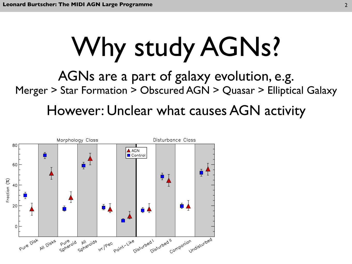
AGNs are a part of galaxy evolution, e.g. Merger > Star Formation > Obscured AGN > Quasar > Elliptical Galaxy

Leonard Burtscher: The MIDI AGN Large Programme
Why study AGNs?
2
AGNs are a part of galaxy evolution, e.g. Merger > Star Formation > Obscured AGN > Quasar > Elliptical Galaxy
However: Unclear what causes AGN activity
Leonard Burtscher: The MIDI AGN Large Programme
Why study AGNs?
2
The Astrophysical Journal, 744:148 (9pp), 2012 January 10 Kocevski et al.
F16
0W (
H)
F77
5W (
i)
Spheroids Disks Mergers / Interactions
Figure 3. Examples of AGN host galaxies that were classified as having spheroid and disk morphologies, as well as two galaxies experiencing disruptive interactions.Thumbnails on the top row are WFC3/IR images taken in the F160W (H) band (rest-frame optical), while those on the bottom row are from ACS/WFC in the F775W(i) band (rest-frame ultraviolet). These images demonstrate that accurately classifying the morphology of these galaxies at z ∼ 2 requires H-band imaging.
Figure 4. Fraction of AGN hosts (red triangles) and control galaxies (blue squares) at 1.5 < z < 2.5 assigned to various morphological and disturbance classes. ThePure Disk class includes only disks without a central bulge. The Pure Disk class is a subsample of the All Disks class, which includes disks with and without a centralbulge. Similarly, the Pure Spheroid class includes only spheroids with no discernible disk component. The All Spheroids class includes both Pure Spheroids and diskgalaxies with a central bulge. The Disturbed I class is limited to heavily disturbed galaxies in a clear merger or interaction. The Disturbed II class includes galaxies inthe Disturbed I class, as well as those showing even minor asymmetries in their morphologies. See the text for details.(A color version of this figure is available in the online journal.)
Table 1Visual Classification Results
Classification AGN Control AGN AGNHosts Galaxies LX < 1043 erg s−1 LX > 1043 erg s−1
Pure disk 16.7+5.3−3.5% 30.1+3.3
−2.9% 21.0+8.0−5.1% 12.5+8.2
−3.7%
All disks 51.4+5.8−5.9% 69.0+2.9
−3.3% 68.4+6.5−8.3% 34.4+9.1
−7.3%
Pure spheroid 27.8+5.8−4.6% 16.9+2.8
−2.2% 18.4+7.9−4.7% 40.6+9.0
−7.9%
All spheroids 62.5+5.3−6.0% 55.7+3.3
−3.4% 65.8+6.7−8.3% 62.5+7.5
−9.1%
Irregular 16.7+5.3−3.5% 18.2+2.9
−2.3% 21.0+8.0−5.1% 06.3+7.3
−2.1%
Point-like 09.7+4.7−2.5% 05.5+2.0
−1.2% 02.6+5.6−0.8% 18.8+8.7
−5.0%
Disturbed I 16.7+5.3−3.5% 15.5+2.8
−2.2% 15.8+7.7−4.2% 18.8+8.7
−5.0%
Disturbed II 44.4+5.9−5.6% 48.4+3.4
−3.4% 36.8+8.3−7.0% 53.1+8.4
−8.8%
Companion 19.4+5.5−3.8% 19.6+3.0
−2.4% 18.4+7.9−4.7% 21.9+8.9
−5.6%
Undisturbed 55.6+5.6−5.9% 52.1+3.3
−3.4% 63.2+7.0−8.3% 46.9+8.7
−8.4%
Notes. The Pure Disk and Pure Spheroid classes are included in the All Disks and All Spheroids classes, respectively. Likewise,the Disturbed I class is a subset of the Disturbed II class.
5
AGNs are a part of galaxy evolution, e.g. Merger > Star Formation > Obscured AGN > Quasar > Elliptical Galaxy
However: Unclear what causes AGN activity

Leonard Burtscher: The MIDI AGN Large Programme
Why study AGNs?
2
The Astrophysical Journal, 744:148 (9pp), 2012 January 10 Kocevski et al.
F16
0W (
H)
F77
5W (
i)
Spheroids Disks Mergers / Interactions
Figure 3. Examples of AGN host galaxies that were classified as having spheroid and disk morphologies, as well as two galaxies experiencing disruptive interactions.Thumbnails on the top row are WFC3/IR images taken in the F160W (H) band (rest-frame optical), while those on the bottom row are from ACS/WFC in the F775W(i) band (rest-frame ultraviolet). These images demonstrate that accurately classifying the morphology of these galaxies at z ∼ 2 requires H-band imaging.
Figure 4. Fraction of AGN hosts (red triangles) and control galaxies (blue squares) at 1.5 < z < 2.5 assigned to various morphological and disturbance classes. ThePure Disk class includes only disks without a central bulge. The Pure Disk class is a subsample of the All Disks class, which includes disks with and without a centralbulge. Similarly, the Pure Spheroid class includes only spheroids with no discernible disk component. The All Spheroids class includes both Pure Spheroids and diskgalaxies with a central bulge. The Disturbed I class is limited to heavily disturbed galaxies in a clear merger or interaction. The Disturbed II class includes galaxies inthe Disturbed I class, as well as those showing even minor asymmetries in their morphologies. See the text for details.(A color version of this figure is available in the online journal.)
Table 1Visual Classification Results
Classification AGN Control AGN AGNHosts Galaxies LX < 1043 erg s−1 LX > 1043 erg s−1
Pure disk 16.7+5.3−3.5% 30.1+3.3
−2.9% 21.0+8.0−5.1% 12.5+8.2
−3.7%
All disks 51.4+5.8−5.9% 69.0+2.9
−3.3% 68.4+6.5−8.3% 34.4+9.1
−7.3%
Pure spheroid 27.8+5.8−4.6% 16.9+2.8
−2.2% 18.4+7.9−4.7% 40.6+9.0
−7.9%
All spheroids 62.5+5.3−6.0% 55.7+3.3
−3.4% 65.8+6.7−8.3% 62.5+7.5
−9.1%
Irregular 16.7+5.3−3.5% 18.2+2.9
−2.3% 21.0+8.0−5.1% 06.3+7.3
−2.1%
Point-like 09.7+4.7−2.5% 05.5+2.0
−1.2% 02.6+5.6−0.8% 18.8+8.7
−5.0%
Disturbed I 16.7+5.3−3.5% 15.5+2.8
−2.2% 15.8+7.7−4.2% 18.8+8.7
−5.0%
Disturbed II 44.4+5.9−5.6% 48.4+3.4
−3.4% 36.8+8.3−7.0% 53.1+8.4
−8.8%
Companion 19.4+5.5−3.8% 19.6+3.0
−2.4% 18.4+7.9−4.7% 21.9+8.9
−5.6%
Undisturbed 55.6+5.6−5.9% 52.1+3.3
−3.4% 63.2+7.0−8.3% 46.9+8.7
−8.4%
Notes. The Pure Disk and Pure Spheroid classes are included in the All Disks and All Spheroids classes, respectively. Likewise,the Disturbed I class is a subset of the Disturbed II class.
5
AGNs are a part of galaxy evolution, e.g. Merger > Star Formation > Obscured AGN > Quasar > Elliptical Galaxy
However: Unclear what causes AGN activityTWO-DIMENSIONAL AGN SIMULATIONS 11
Fig. 6.— Eddington ratio as a function of time, for three different time intervals in the A2 simulation.
3.4. Star Formation and Galactic Winds, and GasContent
Table 1 gives total mass of stars formed, total massof gas driven beyond 10Re, and final mass of gaswithin 10Re for each simulation. Star formation con-sumes about 30% of the total mass budget in the two-dimensional simulations and is very insensitive to thedetails of the AGN feedback. This is in good agreementwith the one-dimensional simulations at low mechanicalefficiencies. However, at high feedback efficiencies, theone-dimensional simulations drive significant quantitiesof gas out of the galaxy, leading to low star formationrates and low final gas content. In this respect the one-dimensional and two-dimensional simulations disagree.However, this is to be expected since assuming sphericalsymmetry gives the most favorable situation for turninga central energy source into a global outflow. In twodimensions, energy can escape via low-density channelsand fail to participate in driving an outflow.
Figure 10 shows the mean mechanical energy inputversus the mean efficiency for one-dimensional and two-dimensional A models. For two-dimensional A models,the energy input is nearly constant—the SMBH accre-tion self-regulates to provide energy at this rate. Theone-dimensional A models have lower energy input rates.That is, two-dimensional models require more energy toreach equilibrium between inflow (due to cooling) andoutflow (due to mechanical feedback).
4. CONCLUSIONS
We have performed two-dimensional simulations of theentire cosmic history (12 Gyr) of an isolated L∗ ellipticalgalaxy. Planetary nebulae and red giant winds producedby evolving low-mass stars serve as the source of gas inthe galaxy. This gas finally ends up either in the centralBH, in long-lived low-mass stars (formed in the simula-tion), in the ISM within the galaxy (at the end of thesimulation), or outside the galaxy as part of the inter-galactic medium. As gas finds its way to one of those four
Variability on „short“ timescales
Leonard Burtscher: The MIDI AGN Large Programme
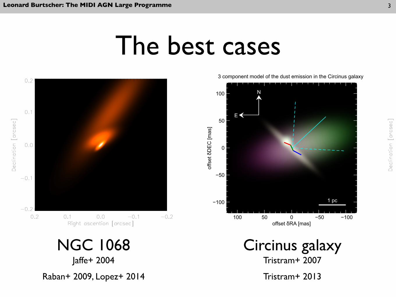
The best cases
3
NGC 1068 Circinus galaxyJaffe+ 2004 Tristram+ 2007
Raban+ 2009, Lopez+ 2014 Tristram+ 2013
1 pc
3 component model of the dust emission in the Circinus galaxy
−100−50050100
offset δRA [mas]
−100
−50
0
50
100
offset
δD
EC
[m
as]
E
N
N. López-Gonzaga et al.: Revealing the large nuclear dust structures in NGC 1068 with MIDI/VLTI
Fig. 8. Image of the No. 1 (Left) and No 2. (Right) best three component models for the mid-infrared emission at 12.0 µm of the nuclear regionof NGC 1068. The image was scaled using the square root of the brightness. Center) Comparison between our first best model and the 12.5 µmimage of Bock et al. (2000), taken with the 10m Keck telescope. The dashed circles represent the FWHM of the field of view for MIDI using theUTs (blue) or the ATs (orange). The letters indicate the positions of the [OIII] clouds according to Evans et al. (1991)
7. The energetics of the mid-infrared emission
The primary scientific results from these observations are thedetection of the “intermediate" components 2 and 3 –1.3 and 7parsecs north of the core–, and the non-detection of the Tongue,about 35 parsec to the north. In this section we consider thepossible heating mechanisms for the dust in these components.
The usual suspects are radiative heating and shock heating.In fact these mechanisms collaborate. The hot gas in a strongshock will be destroy the local dust by sputtering and conduc-tive heating, but it will also emit ultraviolet light that efficientlyheats dust in the surrounding environment. The morphology ofthe emission from the Tongue region supports this combined sce-nario. The VLBA radio images, (Gallimore et al. 2004), show asmall bright component (C) with a sharp edge near this position,suggesting a shock. Most of the radio emission comes from a re-gion less than 30 mas in diameter. Our data, and the images fromGratadour et al. (2006) indicate that the dust emission is comingfrom a much larger region, probably displaced from radio com-ponent C. In particular the MIDI data excludes a narrow ridgemorphology that might be associated with a shock. This ex-tended emission presumably arises from radiatively heated dust.
Wang et al. (2012) describe a similar scenario based on rela-tively high resolution (300 mas) Chandra X-ray data. The X-ray and radio bright region HST-G about 1" north of the nu-cleus shows an X-ray spectrum containing both photoionizedand high-density thermal components. Detailed X-ray spectrafor the other X-ray components in the region are not available,but the ratio of [OIII] to soft X-ray continuum indicates thatsome (labelled HST-D, E, F) are radiation heated, while others(HST-G, H and the near-nuclear region HST-A, B, C) containshocked gas. The HST-A, B, C region contains the nucleus (tothe extent not blocked by Compton scattering), our components1,2, and 3, and the Tongue. Unfortunately the spatial resolutionof the X-ray and [OIII] data cannot distinguish between thesesubcomponents. The very high resolution VLBA data of Gal-limore et al. (2004) show a flat-spectrum nuclear component,presumably coinciding with out component 1, but no emissionat our positions 2 or 3. They find strong synchrotron emission atthe Tongue and at their NE component, which curiously shows
no enhanced X-ray, [OIII] or infrared emission. There are sev-eral regions, e.g. HST-D, E, F of Evans et al. (1991) that showX-ray, [OIII] and infrared emission but where there is no signof shock enhancement of the synchrotron jet (Gallimore et al.2004). Regions NE-5, 6, 7 of Galliano et al. (2005) show thesame features. There is no evidence at these positions of directinteraction with the radio jet, although they lie at the edge of aradio cocoon (Wilson & Ulvestad 1983).
This summary indicates the complexity of the region andsuggests that different mechanisms dominate at different posi-tions. The data from the Tongue region seems to support theshock plus radiative heating in this area. On the other hand, ourregion 3 show no signature of shocks in the radio. This fact andthe proximity to the nucleus favor heating by UV-radiation fromthe nucleus.
We can examine whether the infrared spectral informationin the region is consistent with this hypothesis. The luminosityproduced by the nucleus is sufficient to obtain create the dusttemperature measured at this position. The expected temperatureof dust (assuming silicate grains) heated directly by the centralengine is given by:
T ≃ 1500⎛⎜⎜⎜⎜⎝
Luv,46
r2pc
⎞⎟⎟⎟⎟⎠
15.6
K (4)
where Luv,46 is the luminosity of the heating source in units of1046 erg s−1 (Barvainis 1987). For the central source of NGC1068 we take the UV luminosity Luv = 1.5 × 1045 erg s−1 pre-viously used by Gratadour et al. (2003) to reproduce the centralK band flux and continuum. Dust at a distance of r ∼ 7 pc (100mas) can be heated to T = 530 K. The color temperatures in ourwavelength range are lower, ∼ 400K.
The spectra of the various infrared components show vari-ous, sometime quite high color temperatures, but it is difficult touse this to distinguish radiative from shock heating. The dust inthe shock heated Tongue region shows short wavelength fluxeswith color temperatures ∼ 700K (Gratadour et al. 2006), butsome of the shortest wavelength data may represent scatterednuclear light rather than local thermal emission. The spatial res-olution of the data in Gratadour et al. (2006) is not sufficient to
Article number, page 13 of 21

Leonard Burtscher: The MIDI AGN Large Programme
Building a large sample
4

Leonard Burtscher: The MIDI AGN Large Programme 5
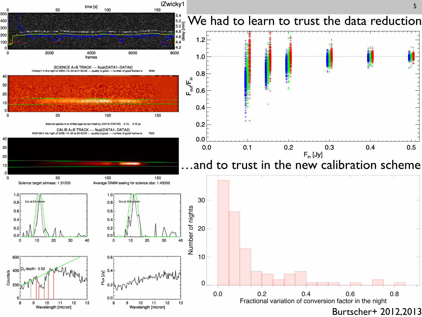
Burtscher+ 2012,2013

Leonard Burtscher: The MIDI AGN Large Programme 5
0.0 0.1 0.2 0.3 0.4 0.5Fin [Jy]
0.0
0.2
0.4
0.6
0.8
1.0
1.2
F out/F
in
0.0 0.1 0.2 0.3 0.4 0.5Fin [Jy]
0.0
0.2
0.4
0.6
0.8
1.0
1.2
F out/F
in
We had to learn to trust the data reduction
Burtscher+ 2012,2013
Leonard Burtscher: The MIDI AGN Large Programme 5
0.0 0.1 0.2 0.3 0.4 0.5Fin [Jy]
0.0
0.2
0.4
0.6
0.8
1.0
1.2
F out/F
in
0.0 0.1 0.2 0.3 0.4 0.5Fin [Jy]
0.0
0.2
0.4
0.6
0.8
1.0
1.2
F out/F
in
We had to learn to trust the data reduction
0.0 0.2 0.4 0.6 0.8Fractional variation of conversion factor in the night
0
10
20
30N
umbe
r of n
ight
s
…and to trust in the new calibration scheme
Burtscher+ 2012,2013

Leonard Burtscher: The MIDI AGN Large Programme
(u,v) coverages [Examples]
6
IC4329A
−100
−50
0
50
100
v [m
]
IC4329A
−100
−50
0
50
100
v [m
]
100 50 0 −50 −1000u [m]
U1U2
U1U3U1U4
U2U3U2U4
U3U4
13 49 19 −30 18 33
LEDA17155
−100
−50
0
50
100
v [m
]
LEDA17155
−100
−50
0
50
100
v [m
]
100 50 0 −50 −1000u [m]
U1U2
U1U3U1U4
U2U3U2U4
U3U4
05 21 01 −25 21 45
MCG−5−23−16
−100
−50
0
50
100
v [m
]
MCG−5−23−16
−100
−50
0
50
100
v [m
]
100 50 0 −50 −1000u [m]
U1U2
U1U3U1U4
U2U3U2U4
U3U4
09 47 40 −30 56 53
NGC1365
−100
−50
0
50
100
v [m
]
NGC1365
−100
−50
0
50
100
v [m
]
100 50 0 −50 −1000u [m]
U1U2
U1U3
U1U4
U2U3
U2U4
U3U4
03 33 36 −36 08 25
Leonard Burtscher: The MIDI AGN Large Programme
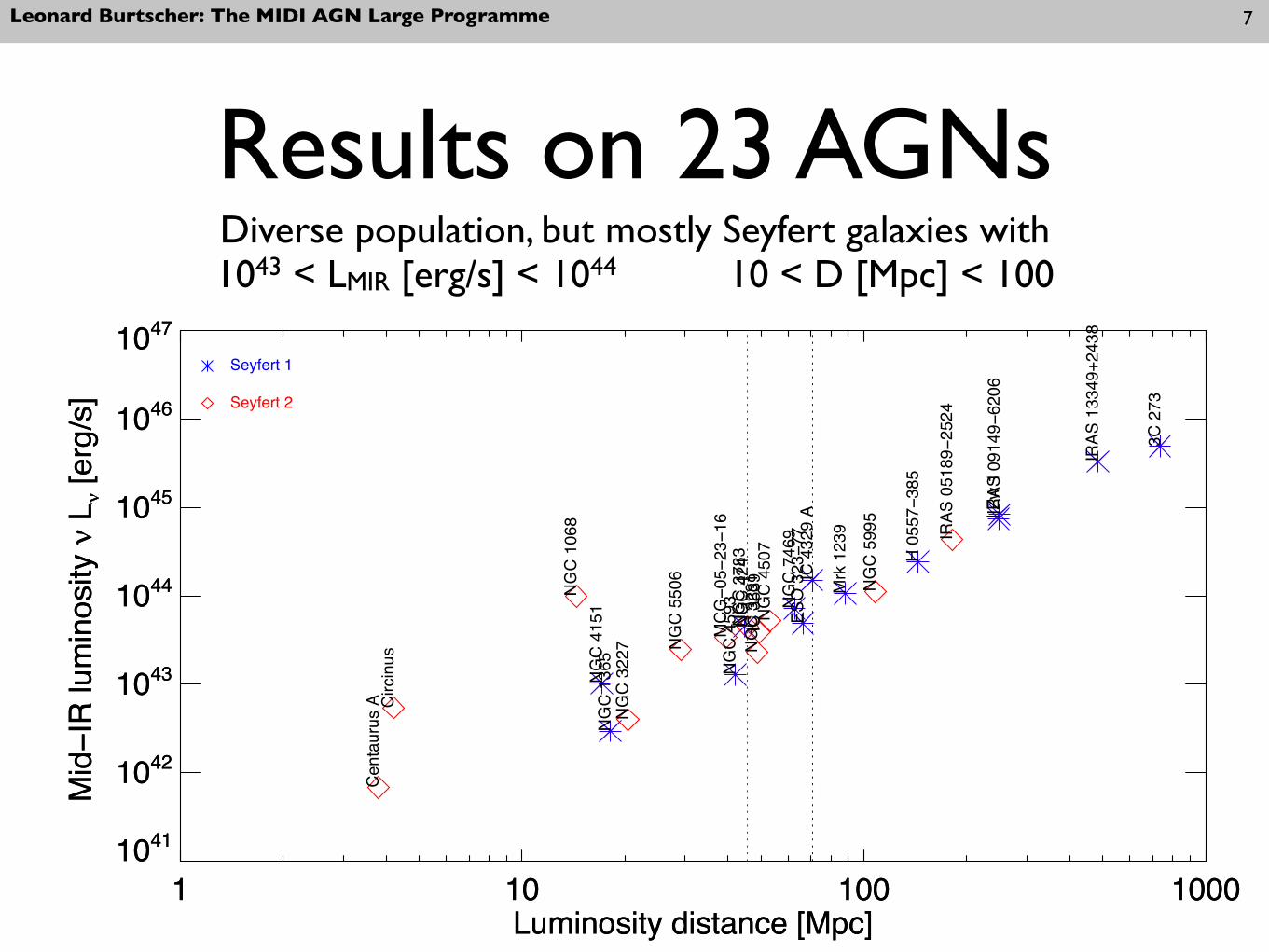
Results on 23 AGNs
7
1 10 100 1000Luminosity distance [Mpc]
1041
1042
1043
1044
1045
1046
1047
Mid−I
R lu
min
osity
ν L
ν [er
g/s]
1 10 100 1000Luminosity distance [Mpc]
1041
1042
1043
1044
1045
1046
1047
Mid−I
R lu
min
osity
ν L
ν [er
g/s]
I Zw
1
NG
C 4
24
NG
C 1
068
NG
C 1
365
IRAS
051
89−2
524
H 0
557−
385
IRAS
091
49−6
206
MC
G−0
5−23−1
6
Mrk
123
9
NG
C 3
281
NG
C 3
783
NG
C 4
151
3C 2
73
NG
C 4
507
NG
C 4
593
ESO
323−7
7
Cen
taur
us A
IRAS
133
49+2
438
IC 4
329
A
Circ
inus
NG
C 5
506 NG
C 5
995
NG
C 7
469
NG
C 3
227
IC 3
639
Seyfert 1
Seyfert 2
Diverse population, but mostly Seyfert galaxies with 1043 < LMIR [erg/s] < 1044 10 < D [Mpc] < 100
Leonard Burtscher: The MIDI AGN Large Programme 8

Leonard Burtscher: The MIDI AGN Large Programme 8

Leonard Burtscher: The MIDI AGN Large Programme 8
Leonard Burtscher: The MIDI AGN Large Programme
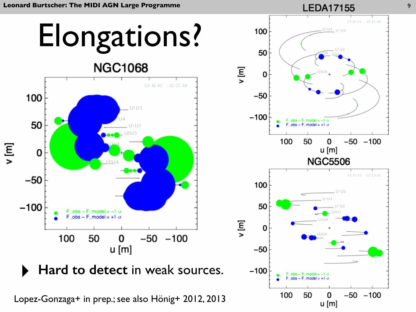
Elongations?9
‣ Hard to detect in weak sources.
Lopez-Gonzaga+ in prep.; see also Hönig+ 2012, 2013
Leonard Burtscher: The MIDI AGN Large Programme 10

Leonard Burtscher: The MIDI AGN Large Programme 10

Leonard Burtscher: The MIDI AGN Large Programme
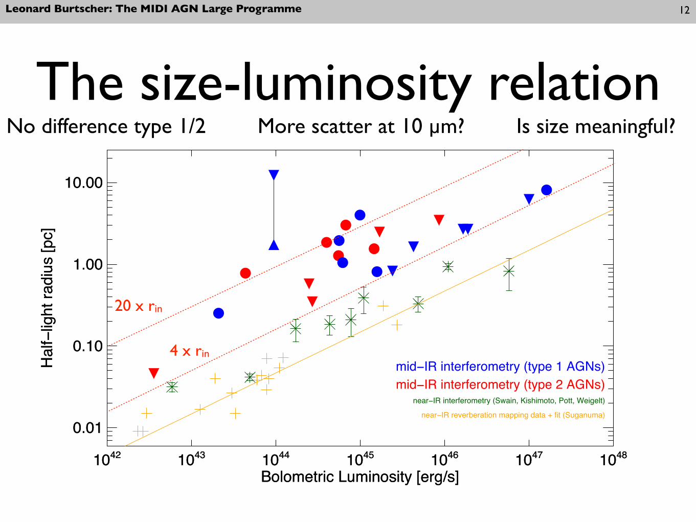
The size-luminosity relation
11
K. R. W. Tristram and M. Schartmann: On the size-luminosity relation of AGN dust tori
Fig. 3. Size of the mid-infrared emitter as afunction of its monochromatic luminosity inthe mid-infrared for type 1 (light blue) andtype 2 (dark blue) AGN. Upper and lower lim-its on the size estimates are marked by arrows.The fitted relation s = p · L0.5 is delineated bythe black continuous line, the scatter in the rela-tion by the dashed lines. The ranges of sizes es-timated from the hydrodynamical torus modelare plotted in orange, those from the clumpytorus model in dark red.
about half of the mid-infrared emission from the same torus seenface-on, even though it is at the same time roughly twice as ex-tended. The discrepancy is about the same for both torus mod-els, hence we consider it to be genuine for all similar toroidaldust distributions. The significance of the discrepancy, how-ever, is stronger for the hydrodynamical model, because for thismodel the uncertainties induced by the assumption of a Gaussianbrightness distribution are smaller. This difference in the appar-ent mid-infrared luminosity of the two orientations of the torushas to be taken into account when evaluating the completeness ofmid-infrared selected AGN samples and the statistics of type 1and type 2 sources in such a sample.
For the same mid-infrared luminosity, a Seyfert 1 torus thusappears about 2.5 times smaller than a Seyfert 2 torus. Its bright-ness distribution appears more compact, because it is dominatedby the bright emission from the hot dust at the inner rim of thetorus, i.e. it has a stronger flux concentration towards the centreof the brightness distribution. This is clearly visible when com-paring the images in the left (torus face-on) and right columns(torus edge-on) of Fig. 1. Because this difference in size is sig-nificant in the sense that it is on the order of or larger than theuncertainty in the size estimates, this should lead to a separa-tion of Seyfert 2 and Seyfert 1 tori into two distinct loci on thesize-luminosity relation. More realistically, there is of course acontinuous distribution of objects between the face-on and edge-on extremes considered here. That is, there should be a gradientwith the object type in the distribution, perpendicular to the di-rection of the relation. However, the scatter in the currently ob-served size estimates show that this assumption does not hold insuch a simple way. The apparent differences in individual objectsare much larger than those of the two classes of objects. With thecurrent data it is thus impossible to ascertain a difference in thecompactness of the type 1 and type 2 tori. With smaller errorsand a larger sample of sources, the statistics may be improvedand a distinction might become possible.
The strong differences in the accuracy of size estimatesderived by employing a Gaussian approximation for the twodifferent torus models are caused by their different radial
brightness distributions. The radial brightness profile of thehydrodynamical model is relatively close to that of a Gaussianprofile (especially for the Seyfert 2 case), while that of theclumpy torus model follows a power law. The scatter in the sizeestimates for a single object from different visibility measure-ments agrees with the uncertainties derived from the models.Furthermore, lower visibilities yield smaller size estimates. Thisagrees well with the monotonically increasing sizes for increas-ing model visibilities found in Sect. 3.3 and indicates that – un-surprisingly – the true brightness distributions deviate from ourGaussian assumption. With more accurate size estimates for dif-ferent visibility measurements, it will hence be possible to dis-tinguish between different radial brightness profiles: a larger dif-ference between the size estimates at different visibilities willindicate that the radial brightness distribution has power-law de-pendence, as in the case of the clumpy torus model. A weakerdependence would imply a more Gaussian-like distribution, sim-ilar to that of the hydrodynamical torus model. This result willcomplement methods directly targeted at the investigation of theradial brightness profile of AGN tori, as for example carried outby Kishimoto et al. (2009a). For this, it will, however, be nec-essary to significantly reduce the error bars in the individual,measured size estimates.
4.2. Size as a function of the estimated intrinsic luminosity
Instead of plotting the size estimates as a function of the lumi-nosity in the mid-infrared, L12 µm, we can also plot the half-size,that is, the mean distance of the dust from the centre r = 0.5 · s,as a function of the intrinsic luminosity of the AGN, using theX-ray luminosities as a proxy. This is shown in Fig. 4 and canbe considered to be the “true” size-luminosity relation and notonly a measure of the compactness of the emission region inthe infrared.
The measurements are again consistent with a relation wherer ∼ L0.5 and we obtain p̃ = (0.76 ± 0.11) × 10−18 pc W−0.5
for the corresponding proportionality constant. This is not sur-prising considering the good correlation between X-ray and
A99, page 7 of 9
Tristram & Schartmann 2011
Tori appear larger when seen edge-on

Leonard Burtscher: The MIDI AGN Large Programme
The size-luminosity relation
12
1042 1043 1044 1045 1046 1047 1048
Bolometric Luminosity [erg/s]
0.01
0.10
1.00
10.00
Half−
light
radi
us [p
c]
1042 1043 1044 1045 1046 1047 1048
Bolometric Luminosity [erg/s]
0.01
0.10
1.00
10.00
Half−
light
radi
us [p
c]
mid−IR interferometry (type 1 AGNs)mid−IR interferometry (type 2 AGNs)
near−IR interferometry (Swain, Kishimoto, Pott, Weigelt)
near−IR reverberation mapping data + fit (Suganuma)
No difference type 1/2

Leonard Burtscher: The MIDI AGN Large Programme
The size-luminosity relation
12
1042 1043 1044 1045 1046 1047 1048
Bolometric Luminosity [erg/s]
0.01
0.10
1.00
10.00
Half−
light
radi
us [p
c]
1042 1043 1044 1045 1046 1047 1048
Bolometric Luminosity [erg/s]
0.01
0.10
1.00
10.00
Half−
light
radi
us [p
c]
mid−IR interferometry (type 1 AGNs)mid−IR interferometry (type 2 AGNs)
near−IR interferometry (Swain, Kishimoto, Pott, Weigelt)
near−IR reverberation mapping data + fit (Suganuma)
4 x rin
20 x rin
More scatter at 10 µm?No difference type 1/2
Leonard Burtscher: The MIDI AGN Large Programme
The size-luminosity relation
12
1042 1043 1044 1045 1046 1047 1048
Bolometric Luminosity [erg/s]
0.01
0.10
1.00
10.00
Half−
light
radi
us [p
c]
1042 1043 1044 1045 1046 1047 1048
Bolometric Luminosity [erg/s]
0.01
0.10
1.00
10.00
Half−
light
radi
us [p
c]
mid−IR interferometry (type 1 AGNs)mid−IR interferometry (type 2 AGNs)
near−IR interferometry (Swain, Kishimoto, Pott, Weigelt)
near−IR reverberation mapping data + fit (Suganuma)
4 x rin
20 x rin
More scatter at 10 µm?No difference type 1/2 Is size meaningful?

Leonard Burtscher: The MIDI AGN Large Programme 13
Schartmann et al. 2008
The fraction of unresolved flux…does not depend much on inclination or position angle12 M. Schartmann et al.: Three-dimensional radiative transfer models of clumpy tori in Seyfert galaxies
Fig. 18. Visibilities of our continuous standard model at a wave-length of 12 µm plotted against the projected baseline length.Colour of the visibility distributions refers to different positionangles of the projected baseline w. r. t. the torus axis. Each panelshows a different inclination angle, as indicated in the upper rightcorner.
Seyfert galaxies. MIDI is designed as a classical Michelson in-terferometer. Being a two-element beam combining instrument,it measures so-called visibility amplitudes. Visibility is definedas the ratio between the correlated flux and the total flux. Its in-terpretation is not straightforward, since no direct image can bereconstructed. Therefore, a model has to be assumed, which canthen be compared to the visibility data. MIDI works in dispersedmode, which means that visibilities for the whole wavelengthrange are derived. The dust emission is probed depending on theorientation of the projected baseline. Point-like objects result ina visibility of one, as the correlated flux equals the total flux.The more extended the object, the lower the visibility. With thehelp of a density distribution, surface brightness distributions inthe mid-infrared can be calculated by applying a radiative trans-fer code. A Fourier transform of the brightness distribution thenyields the visibility information, depending on the baseline ori-entation and length within the so-called U-V-plane (or Fourier-plane).
The main goal of the following analysis is to investigatewhether MIDI can distinguish between clumpy and continuoustorus models of the kind presented above. Furthermore, we try toderive characteristic features of the respective models and showa comparison to data obtained for the Circinus galaxy.
6.1. Model visibilities
In Fig. 18, calculated visibilities for four inclinations of our con-tinuous standard model at a wavelength of λ= 12 µm are shown.Various orientations of the projected baseline are colour coded(the given position angle is counted anti-clockwise from the pro-jected torus axis). Due to the axisymmetric setup, all lines coin-cide for the face-on case. For all other inclination angles, visibili-
Fig. 19. Visibilities of our clumpy standard model at a wave-length of 12 µm plotted against the projected baseline length.Colour of the visibility distributions refers to different positionangles of the baseline w. r. t. the torus axis. Each panel shows adifferent inclination angle, as indicated in the upper right corner.
ties decrease until a position angle of 90◦ is reached and increasesymmetrically again. This means that the torus appears elon-gated perpendicular to the torus axis at this wavelength. Fig. 19shows the same study, but for the corresponding clumpy model.The basic behaviour is the same, but the visibilities show finestructure and the scatter is much greater, especially visible inthe comparison of the i = 0◦ cases. Furthermore, while all ofthe curves of the continuous model monotonically decrease withbaseline length, we see rising and falling values with increasingbaseline length for the same position angle in the clumpy case.In addition, for the continuous models, curves do not intersect,in contrast to our clumpy models. However, to detect such finestructure in observedMIDI data, a very high accuracy in the vis-ibility measurements of the order of σv ≈ 0.02 and a very densesampling is required.
In Fig. 20, the wavelength dependence of the visibilities isshown. The first two panels represent the case of the clumpystandard model and the third and fourth the continuous model.Each of the two panels of the respective model visualises a dif-ferent position angle (counted anti-clockwise from the projectedtorus axis). An inclination angle of 90◦ is used in all panels.Three different wavelengths are colour coded: 8.2 µm at the be-ginning of the MIDI-range (black dotted line), 9.8 µmwithin thesilicate feature (blue) and 12.6 µm at the end of the MIDI wave-length range (yellow), outside the silicate feature.While the con-tinuous model results in smooth curves (see also Fig. 18), muchfine structure is visible for the case of the clumpy model. Thedifferences between the displayed wavelengths relative to thelongest wavelength are smaller for the clumpy models than inthe continuous case.
Fig. 21 shows visibilities for our clumpy standard modelat 12 µm, plotted against the position angle (counter-clockwisefrom the projected torus axis). Baselines are colour coded be-
12 M. Schartmann et al.: Three-dimensional radiative transfer models of clumpy tori in Seyfert galaxies
Fig. 18. Visibilities of our continuous standard model at a wave-length of 12 µm plotted against the projected baseline length.Colour of the visibility distributions refers to different positionangles of the projected baseline w. r. t. the torus axis. Each panelshows a different inclination angle, as indicated in the upper rightcorner.
Seyfert galaxies. MIDI is designed as a classical Michelson in-terferometer. Being a two-element beam combining instrument,it measures so-called visibility amplitudes. Visibility is definedas the ratio between the correlated flux and the total flux. Its in-terpretation is not straightforward, since no direct image can bereconstructed. Therefore, a model has to be assumed, which canthen be compared to the visibility data. MIDI works in dispersedmode, which means that visibilities for the whole wavelengthrange are derived. The dust emission is probed depending on theorientation of the projected baseline. Point-like objects result ina visibility of one, as the correlated flux equals the total flux.The more extended the object, the lower the visibility. With thehelp of a density distribution, surface brightness distributions inthe mid-infrared can be calculated by applying a radiative trans-fer code. A Fourier transform of the brightness distribution thenyields the visibility information, depending on the baseline ori-entation and length within the so-called U-V-plane (or Fourier-plane).
The main goal of the following analysis is to investigatewhether MIDI can distinguish between clumpy and continuoustorus models of the kind presented above. Furthermore, we try toderive characteristic features of the respective models and showa comparison to data obtained for the Circinus galaxy.
6.1. Model visibilities
In Fig. 18, calculated visibilities for four inclinations of our con-tinuous standard model at a wavelength of λ= 12 µm are shown.Various orientations of the projected baseline are colour coded(the given position angle is counted anti-clockwise from the pro-jected torus axis). Due to the axisymmetric setup, all lines coin-cide for the face-on case. For all other inclination angles, visibili-
Fig. 19. Visibilities of our clumpy standard model at a wave-length of 12 µm plotted against the projected baseline length.Colour of the visibility distributions refers to different positionangles of the baseline w. r. t. the torus axis. Each panel shows adifferent inclination angle, as indicated in the upper right corner.
ties decrease until a position angle of 90◦ is reached and increasesymmetrically again. This means that the torus appears elon-gated perpendicular to the torus axis at this wavelength. Fig. 19shows the same study, but for the corresponding clumpy model.The basic behaviour is the same, but the visibilities show finestructure and the scatter is much greater, especially visible inthe comparison of the i = 0◦ cases. Furthermore, while all ofthe curves of the continuous model monotonically decrease withbaseline length, we see rising and falling values with increasingbaseline length for the same position angle in the clumpy case.In addition, for the continuous models, curves do not intersect,in contrast to our clumpy models. However, to detect such finestructure in observedMIDI data, a very high accuracy in the vis-ibility measurements of the order of σv ≈ 0.02 and a very densesampling is required.
In Fig. 20, the wavelength dependence of the visibilities isshown. The first two panels represent the case of the clumpystandard model and the third and fourth the continuous model.Each of the two panels of the respective model visualises a dif-ferent position angle (counted anti-clockwise from the projectedtorus axis). An inclination angle of 90◦ is used in all panels.Three different wavelengths are colour coded: 8.2 µm at the be-ginning of the MIDI-range (black dotted line), 9.8 µmwithin thesilicate feature (blue) and 12.6 µm at the end of the MIDI wave-length range (yellow), outside the silicate feature.While the con-tinuous model results in smooth curves (see also Fig. 18), muchfine structure is visible for the case of the clumpy model. Thedifferences between the displayed wavelengths relative to thelongest wavelength are smaller for the clumpy models than inthe continuous case.
Fig. 21 shows visibilities for our clumpy standard modelat 12 µm, plotted against the position angle (counter-clockwisefrom the projected torus axis). Baselines are colour coded be-
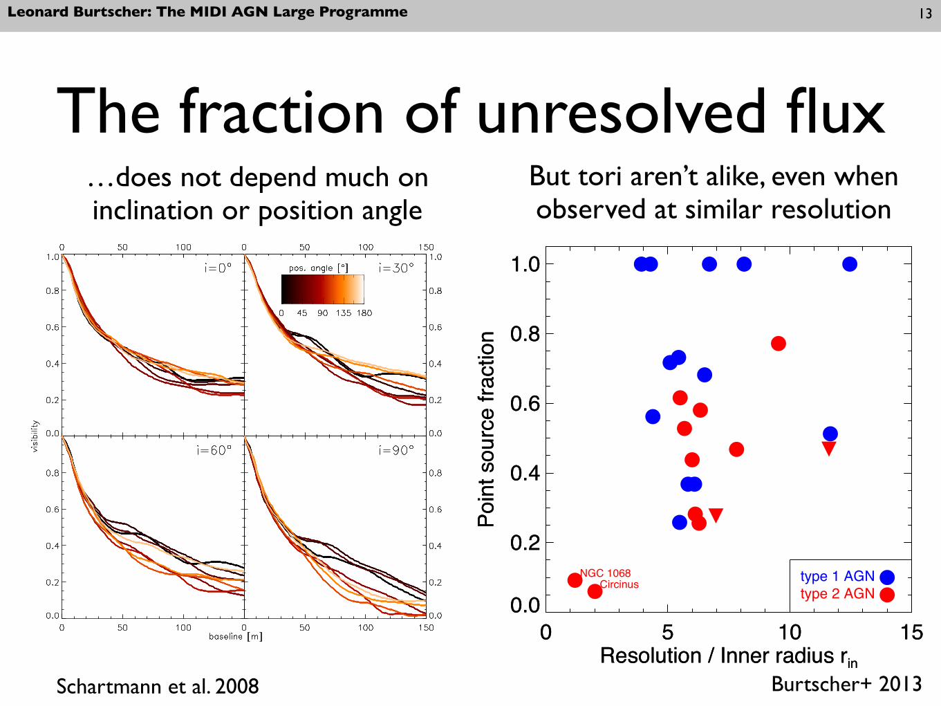
Leonard Burtscher: The MIDI AGN Large Programme 13
Schartmann et al. 2008
The fraction of unresolved flux…does not depend much on inclination or position angle
0 5 10 15Resolution / Inner radius rin
0.0
0.2
0.4
0.6
0.8
1.0
Poin
t sou
rce
fract
ion
0 5 10 15Resolution / Inner radius rin
0.0
0.2
0.4
0.6
0.8
1.0
Poin
t sou
rce
fract
ion
NGC 1068Circinus type 1 AGN
type 2 AGN
Burtscher+ 2013
But tori aren’t alike, even when observed at similar resolution12 M. Schartmann et al.: Three-dimensional radiative transfer models of clumpy tori in Seyfert galaxies
Fig. 18. Visibilities of our continuous standard model at a wave-length of 12 µm plotted against the projected baseline length.Colour of the visibility distributions refers to different positionangles of the projected baseline w. r. t. the torus axis. Each panelshows a different inclination angle, as indicated in the upper rightcorner.
Seyfert galaxies. MIDI is designed as a classical Michelson in-terferometer. Being a two-element beam combining instrument,it measures so-called visibility amplitudes. Visibility is definedas the ratio between the correlated flux and the total flux. Its in-terpretation is not straightforward, since no direct image can bereconstructed. Therefore, a model has to be assumed, which canthen be compared to the visibility data. MIDI works in dispersedmode, which means that visibilities for the whole wavelengthrange are derived. The dust emission is probed depending on theorientation of the projected baseline. Point-like objects result ina visibility of one, as the correlated flux equals the total flux.The more extended the object, the lower the visibility. With thehelp of a density distribution, surface brightness distributions inthe mid-infrared can be calculated by applying a radiative trans-fer code. A Fourier transform of the brightness distribution thenyields the visibility information, depending on the baseline ori-entation and length within the so-called U-V-plane (or Fourier-plane).
The main goal of the following analysis is to investigatewhether MIDI can distinguish between clumpy and continuoustorus models of the kind presented above. Furthermore, we try toderive characteristic features of the respective models and showa comparison to data obtained for the Circinus galaxy.
6.1. Model visibilities
In Fig. 18, calculated visibilities for four inclinations of our con-tinuous standard model at a wavelength of λ= 12 µm are shown.Various orientations of the projected baseline are colour coded(the given position angle is counted anti-clockwise from the pro-jected torus axis). Due to the axisymmetric setup, all lines coin-cide for the face-on case. For all other inclination angles, visibili-
Fig. 19. Visibilities of our clumpy standard model at a wave-length of 12 µm plotted against the projected baseline length.Colour of the visibility distributions refers to different positionangles of the baseline w. r. t. the torus axis. Each panel shows adifferent inclination angle, as indicated in the upper right corner.
ties decrease until a position angle of 90◦ is reached and increasesymmetrically again. This means that the torus appears elon-gated perpendicular to the torus axis at this wavelength. Fig. 19shows the same study, but for the corresponding clumpy model.The basic behaviour is the same, but the visibilities show finestructure and the scatter is much greater, especially visible inthe comparison of the i = 0◦ cases. Furthermore, while all ofthe curves of the continuous model monotonically decrease withbaseline length, we see rising and falling values with increasingbaseline length for the same position angle in the clumpy case.In addition, for the continuous models, curves do not intersect,in contrast to our clumpy models. However, to detect such finestructure in observedMIDI data, a very high accuracy in the vis-ibility measurements of the order of σv ≈ 0.02 and a very densesampling is required.
In Fig. 20, the wavelength dependence of the visibilities isshown. The first two panels represent the case of the clumpystandard model and the third and fourth the continuous model.Each of the two panels of the respective model visualises a dif-ferent position angle (counted anti-clockwise from the projectedtorus axis). An inclination angle of 90◦ is used in all panels.Three different wavelengths are colour coded: 8.2 µm at the be-ginning of the MIDI-range (black dotted line), 9.8 µmwithin thesilicate feature (blue) and 12.6 µm at the end of the MIDI wave-length range (yellow), outside the silicate feature.While the con-tinuous model results in smooth curves (see also Fig. 18), muchfine structure is visible for the case of the clumpy model. Thedifferences between the displayed wavelengths relative to thelongest wavelength are smaller for the clumpy models than inthe continuous case.
Fig. 21 shows visibilities for our clumpy standard modelat 12 µm, plotted against the position angle (counter-clockwisefrom the projected torus axis). Baselines are colour coded be-
12 M. Schartmann et al.: Three-dimensional radiative transfer models of clumpy tori in Seyfert galaxies
Fig. 18. Visibilities of our continuous standard model at a wave-length of 12 µm plotted against the projected baseline length.Colour of the visibility distributions refers to different positionangles of the projected baseline w. r. t. the torus axis. Each panelshows a different inclination angle, as indicated in the upper rightcorner.
Seyfert galaxies. MIDI is designed as a classical Michelson in-terferometer. Being a two-element beam combining instrument,it measures so-called visibility amplitudes. Visibility is definedas the ratio between the correlated flux and the total flux. Its in-terpretation is not straightforward, since no direct image can bereconstructed. Therefore, a model has to be assumed, which canthen be compared to the visibility data. MIDI works in dispersedmode, which means that visibilities for the whole wavelengthrange are derived. The dust emission is probed depending on theorientation of the projected baseline. Point-like objects result ina visibility of one, as the correlated flux equals the total flux.The more extended the object, the lower the visibility. With thehelp of a density distribution, surface brightness distributions inthe mid-infrared can be calculated by applying a radiative trans-fer code. A Fourier transform of the brightness distribution thenyields the visibility information, depending on the baseline ori-entation and length within the so-called U-V-plane (or Fourier-plane).
The main goal of the following analysis is to investigatewhether MIDI can distinguish between clumpy and continuoustorus models of the kind presented above. Furthermore, we try toderive characteristic features of the respective models and showa comparison to data obtained for the Circinus galaxy.
6.1. Model visibilities
In Fig. 18, calculated visibilities for four inclinations of our con-tinuous standard model at a wavelength of λ= 12 µm are shown.Various orientations of the projected baseline are colour coded(the given position angle is counted anti-clockwise from the pro-jected torus axis). Due to the axisymmetric setup, all lines coin-cide for the face-on case. For all other inclination angles, visibili-
Fig. 19. Visibilities of our clumpy standard model at a wave-length of 12 µm plotted against the projected baseline length.Colour of the visibility distributions refers to different positionangles of the baseline w. r. t. the torus axis. Each panel shows adifferent inclination angle, as indicated in the upper right corner.
ties decrease until a position angle of 90◦ is reached and increasesymmetrically again. This means that the torus appears elon-gated perpendicular to the torus axis at this wavelength. Fig. 19shows the same study, but for the corresponding clumpy model.The basic behaviour is the same, but the visibilities show finestructure and the scatter is much greater, especially visible inthe comparison of the i = 0◦ cases. Furthermore, while all ofthe curves of the continuous model monotonically decrease withbaseline length, we see rising and falling values with increasingbaseline length for the same position angle in the clumpy case.In addition, for the continuous models, curves do not intersect,in contrast to our clumpy models. However, to detect such finestructure in observedMIDI data, a very high accuracy in the vis-ibility measurements of the order of σv ≈ 0.02 and a very densesampling is required.
In Fig. 20, the wavelength dependence of the visibilities isshown. The first two panels represent the case of the clumpystandard model and the third and fourth the continuous model.Each of the two panels of the respective model visualises a dif-ferent position angle (counted anti-clockwise from the projectedtorus axis). An inclination angle of 90◦ is used in all panels.Three different wavelengths are colour coded: 8.2 µm at the be-ginning of the MIDI-range (black dotted line), 9.8 µmwithin thesilicate feature (blue) and 12.6 µm at the end of the MIDI wave-length range (yellow), outside the silicate feature.While the con-tinuous model results in smooth curves (see also Fig. 18), muchfine structure is visible for the case of the clumpy model. Thedifferences between the displayed wavelengths relative to thelongest wavelength are smaller for the clumpy models than inthe continuous case.
Fig. 21 shows visibilities for our clumpy standard modelat 12 µm, plotted against the position angle (counter-clockwisefrom the projected torus axis). Baselines are colour coded be-

Leonard Burtscher: The MIDI AGN Large Programme
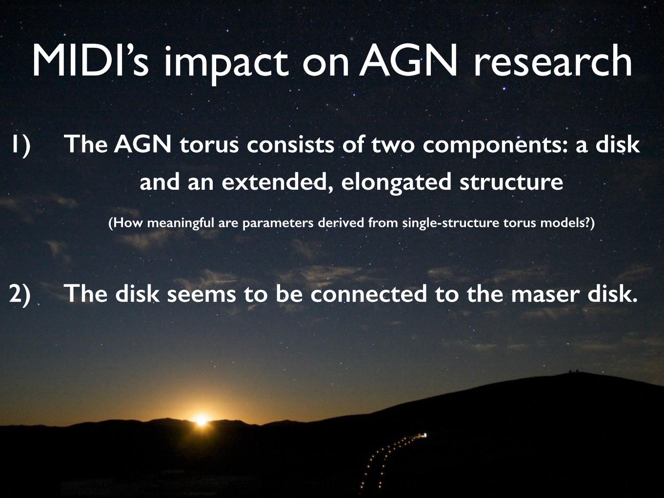
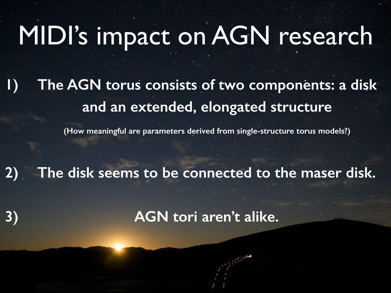
MIDI’s impact on AGN research14

Leonard Burtscher: The MIDI AGN Large Programme
MIDI’s impact on AGN research14
1) The AGN torus consists of two components: a disk and an extended, elongated structure
(How meaningful are parameters derived from single-structure torus models?)
Leonard Burtscher: The MIDI AGN Large Programme
MIDI’s impact on AGN research14
1) The AGN torus consists of two components: a disk and an extended, elongated structure
(How meaningful are parameters derived from single-structure torus models?)
2) The disk seems to be connected to the maser disk.
Leonard Burtscher: The MIDI AGN Large Programme
MIDI’s impact on AGN research14
1) The AGN torus consists of two components: a disk and an extended, elongated structure
(How meaningful are parameters derived from single-structure torus models?)
2) The disk seems to be connected to the maser disk.
3) AGN tori aren’t alike.