Microfinance in Bosnia and Herzegovina

A randomised field experiment on the impact of

extending microfinance to marginal clients

Britta Augsburg (IFS), Ralph De Haas (EBRD), Heike

Harmgart (EBRD) and Costas Meghir (UCL and IFS)

Baseline Report February 2010

1

Contents 1. Introduction 2. Background to the project

2.1. Description of the project and the microfinance market in Bosnia 2.1.1. The microfinance market in Bosnia

2.1.2. Identification of the target population – the “marginal clients” 2.1.3. The interview

2.2. Data 3. Comparison between treatment and control units

3.1. Overview of the sample 3.2. Characteristics of the (potential) marginal clients 3.3. Household characteristics

4. Comparison to total population of Bosnia & Herzegovina 4.1. Individual characteristics 4.2. Household characteristics 4.3. Poverty

5. Socio-economic household indicators 5. 1. Household consumption

5.1.1. Food consumption in the past week 5.1.2. Consumption of other non-durables in the past month 5.1.3. Consumption of other durables in the past year

5.2. Household assets 5.3. Household income 5.4. Household savings 5.5. Shocks experienced by the households

6. Household business and loans 6.1. Household business

6.1.1. Expected business profit 6.2. Household debts 6.3. EKI loan

7. Perception / Stress 7.1. Perception of financial situation 7.2. Stress

8. Conclusions 9. Loan officer’s view of marginal clients 9.1. Expectations 10. Site visit forms

2

APPENDICES

A1 – Presentation for loan officer training A2 – Loan officer guide for the EKI-EBRD microfinance study

A3 – Branch manager guide for the EKI-EBRD microfinance study

B - Expected outcomes, sample design and precision C – Characteristics of female marginal clients D – Socio-economic household indicators E – Third loans of marginal clients

F – Stress questions

3

1. Introduction This report provides a description of the first wave of household data collected for a

randomised field experiment in Bosnia (‘the study’). The study intends to measure the

impact of microcredit on poverty reduction among Bosnian households and the

development of small enterprises that may otherwise not have access to finance.

Microfinance has attracted a lot of attention worldwide as a tool for generating pro-

poor growth and microfinance institutions (MFIs) in many countries have

consequently grown rapidly over recent years. Whereas commercial banks are often

reluctant to advance small uncollateralized loans, MFIs disburse loans that typically

are very small and lack collateral. There have been a number of schemes devised

around the world to guarantee good repayment in the absence of collateral. These

include group lending with joint monitoring and responsibility, and lending to women

(who have a better reputation for repaying).

By providing loans to poor individuals with small family enterprises, microfinance

may allow such businesses to increase their investments and to smooth operations and

consumption. As a result, microfinance is often seen as a key measure to alleviate

poverty in a sustainable way. Yet, hard evidence on the impact of microfinance is still

limited (Banerjee et al., 2009; Karlan and Zinnman, 2009).1 To what extent does

microfinance actually lift people out of poverty, in particular by allowing households

to generate income through small-scale enterprises? This study intends to add to the

empirical evidence that can be brought to bear to answer this question.

Microfinance was introduced in Bosnia in the mid 1990s after the signing of the 1995

Dayton Peace Agreement. Sector support was mainly given by the World Bank via its

funding of a so-called local initiative project. This project trained and supported a

large number of MFIs in Bosnia and the ones that turned out commercially viable

were supported for several more years. Since then, MFIs have provided funds to many

households and small enterprises that may otherwise have remained cut off from any

formal financing. Non-experimental empirical evidence for Bosnia and Herzegovina

indeed suggests that the presence of MFIs has reduced the sensitivity of firms’

investment to changes in their internal funding (Hartarska and Nadolnyak, 2007).

1 The literature on microfinance is reviewed extensively in Armendariz and Murdoch (2005).

4

The percentage of non-performing loans in Bosnian microlending portfolios has

historically been very low and microfinance has become a sustainable though

increasingly competitive business. During recent years a number of commercial banks

‘scaled down’ to get involved in the higher end of the microfinance market, thereby

further adding to the competitive pressure in the Bosnian microfinance market.

Strong competition has encouraged institutions to look for a broader client base

instead of competing for the same (limited) pool of clients. This has become

particularly urgent over recent years when it became increasingly clear that many

Bosnian households had been able to take out loans from various microfinance

providers at the same time, exploiting the fact that a well-functioning credit bureau

was until recently absent.

Against this background, this study entails an experimental intervention during which

– for a limited period of time – loans are given to poorer, still underserved clients

across Bosnia (with possibly somewhat higher credit risk). The ultimate aim of the

evaluation is to (a) measure the effect of extending loans to poorer groups in Bosnia

and (b) to analyse the profitability of such a programme.

The potential conclusions of this project can be:

I. Microfinance reduces poverty of the new client group and continues to be

profitable.

II. Microfinance does not reduce poverty of the new client group but is profitable

within that group.

III. Microfinance reduces poverty of the new client group but is not profitable

within that group.

IV. None of the above.

Under case I and II, the MFI that participates in the study will wish to extend its client

base to this newer riskier group while under III and IV it will not. However, under

case III, while the MFI involved may not be willing to continue to extend such credit,

other sources of funding may be sought if it can be argued that this is a cost effective

way of reducing poverty in the Bosnian context.

The fact that the evaluation will not only measure the impact on the borrower but also

the commercial viability of deepening the MFIs outreach to this new group is a

5

particularly important point because it addresses directly the issue of how the

extension of lending should be financed if considered desirable.

The MFI participating in the field experiment is EKI (http://eki.ba/en/). Initially, the

design entailed cooperation with two Bosnian MFIs, both of which were interested in

introducing a credit scoring system. Participation in this study will help facilitate the

introduction of credit scoring as the repayment data that are generated during the

experiment may be fed into the calibration of such a system. However, the second

MFI had to drop out of the study because of various other projects it was involved in.

As a result, the experiment focused on EKI alone and the EKI sample size was

subsequently scaled up.

The remainder of this report analyses the data that were collected during the first of

two households studies (the baseline survey). We provide statistics that describe our

household sample along a wide range of dimensions such as education, assets,

savings, debt, income, enterprises, consumption and transfers. The analysis of this

population is of interest in its own right and gives a first snapshot of the target

population which is not available from existing data sources. We show formal

comparisons of these characteristics between treatment and control groups, an

important validation test for the randomisation process.

The remainder of this report is structured as follows. Section 2 provides background

information and. Section 3 then compares the two groups of the target population:

those that were chosen to receive a loan and those that were not. The project

population is also compared to the wider population of Bosnia and Herzegovina

(Section 4). In Section 5, we look at socio-economic household indicators and in

Section 6 we discuss the household business and previous loans. The following

section looks at perceptions of the financial situation as well as stress and Section 8

concludes. Section 9 analyses the loan officers’ view of marginal clients and in the

final section we discuss some information that is collected by loan officers when they

visited the potential clients as part of their loan appraisal procedure.

6

2. Background

2.1. Description of the project and the microfinance market in Bosnia

2.1.1. The microfinance market in Bosnia – demand and supply

The legacy of the Dayton Accords still significantly affects the business climate in

BiH. According to the EBRDs business environment and enterprise performance

survey (BEEPS 2009), one quarter of firms consider political instability to be the most

severe obstacle to their business’ performance. Lacking government effectiveness and

harmonization of policies, excessive bureaucracy and continuous ethnic fragmentation

are major impediments small and medium sized enterprises (MSMEs) are confronted

with, and they cannot operate under the same conditions at various locations across

the country. Reflecting on the weak rule of law, enterprises also suffer from the

persistence of the grey economy and wide-spread corruption, such as reflected in the

Transparency International CPI, which ranks BiH the lowest within the Western

Balkan region.

The World Bank Doing Business Report 2010 further highlights the difficult business

environment and ranks BiH 116th, below all other countries in the SEE region.

Actions have been taken to simplify business registration, but a single valid

registration for the whole country is not yet operational and starting a business

remains the biggest obstacle in the Doing Business. In addition, in spite of good

progress made in the previous year in terms of registering property and paying taxes,

these two aspects remain amongst the most severe problems. On the positive side, the

report assesses the environment in BiH relatively well with regard to getting credit,

trading across borders and closing of business.

Doing Business– regional comparison

020406080

100120140160180

Alb

ania

Bos

nia

and

Her

z.

Cro

atia

FYR

Mac

edon

ia

Kos

ovo

Mon

tene

gro

Serb

ia

2009 2010

Doing Business 2010 by subcategories

0

60

120

180Starting a Business

Construction Permits

Employing Workers

Registering Property

Getting Credit

Protecting Investors

Paying Taxes

ading across Borders

Enforcing Contracts

Closing a Business

7

After several years of growth, total assets of the banking sector have stagnated in

2009. Credit growth stood at -3.1 per cent as of December 2009 and the share of

NPLs is expected to have accelerated. Within the context of a Stand-by Agreement

with the IMF, the so-called “Vienna Initiative”, under which several foreign-owned

banks (which dominate the banking sector) have committed themselves to maintain

their exposure in BiH, has ensured stability within the banking sector.

Good progress has been made with the Microfinance Law of 2007, which enables

state banking agencies to supervise micro credit and leasing companies. Micro finance

institutions (MFIs) have expanded significantly in recent years. As a result of the

global downturn, however, payment capacities have decreased and MFI lending has

become more restricted and competition among micro finance institutions has

increased.

Total assets

13%1%

9%

5%

2%

0%

15%

12%5%

28%

3%6% 1%

EKILIDERLOK Microcredit FoundationMI-BOSPOMIKRAMikro ALDIMIKROFINPartnerPRIZMAProCredit Bank - BIHSINERGIJASunriseWomen for Women

Source MiX, Microfinance Information Exchange, 2008 data.

According to BEEPS, around 10 per cent of enterprises surveyed consider access to

finance the most severe obstacle to a smooth business performance and overall access

of the private sector to capital markets remains limited. There is no clear definition of

collateral and micro-loans can be extended in the absence of collateral. In addition, a

registry for pledged movable assets, which anyone can enter information into, became

8

operational in 2006. Lastly, a credit registry exists and is comparatively well

functioning, but individual’s access to their own data is not guaranteed by law.

2.1.2. Identification of the target population – the “marginal clients”

The study consists of identifying potential marginal clients and offering loans to a

random subset of these potential clients (the treatment group). The individuals

randomised out of the intervention – i.e. those that did not receive a loan – make up

the control group.

In a first step, loan officers across all EKI branches were instructed to come up with a

group of potential marginal clients. During training sessions loan officers were

explained that they needed to find clients that they would normally reject, but to

whom they would consider extending loans if they were asked to take up slightly

more risk. The approach was used because EKI does not yet have a formal credit

scoring system in place. Loan officers thus need to use their judgement – as they also

have to in their normal day-to-day procedures – in deciding who is a potential

marginal client rather than a ‘good’ or outright ‘bad’ potential client. While one may

be concerned that the loan officers divert normal clients to the marginal group, this

concern is mitigated by the fact that the loan officers would not want to risk loosing a

solid client via the lottery system for the randomisation.

To facilitate the identification process of potential marginal clients, all EKI loan

officers and branch managers were given training by EBRD and IFS staff who

travelled through Bosnia to give presentations to the different branches. In this

training, information on the project was given, the process was explained and the

questionnaires discussed. Emphasis was put on describing not only why but also how

loan officers could and should relax selection criteria for the project. This same

information was then enforced through meetings of branch managers and EKI

management, of which the outcome was passed on to the loan officers. Finally, the

loan officers also received a document, describing the procedure in detail. Appendix

A contains details on the training (presentation and hand-out).

Once a loan officer identified a potential “marginal client”, (s)he was informed by the

loan officer about the study and the implications, namely that s(he) would normally

not be offered a loan by EKI but that, if agreeing to be interviewed now and in one

9

year’s time, s(he) would have a chance of getting a loan. All potential marginal clients

who agreed to be interviewed were also given a clock as a token of appreciation.

If the potential clients agreed, the loan officer followed the usual application

procedures and submitted the application to the institution’s loan committee. The

committee discussed the applicant (applying slightly different guidelines than for their

‘normal’ clients) and, if considered suitable for the study, the potential marginal client

would be interviewed by PULS, the assigned data collection agency.

Once the population of potentially eligible clients was identified, the allocation to

either the treatment (receiving a loan) or the control group (not receiving a loan) was

carried out weekly on Friday by the IFS and EBRD in London by using a random

number generator. The results of the randomisation were then communicated to EKI,

after which those potential marginal clients that were allocated into the treatment

group could be contacted during the next week by an EKI loan officer to disburse the

loan. Potential marginal clients that were allocated to the control group were not

visited by an EKI officer and did, for the duration of the study, not receive a loan.

2.1.3. The interview

Interviews were conducted by BFC/PULS over the phone. The pilot of the procedure

started on November 24th 2008 in two of the 14 branches. Piloting of the

questionnaire was conducted in the week before the procedure piloting and changes to

the survey were only minimal. On December 15th the experiment was extended to all

branches. The last interview took place on May 5th 2009.

The focus of the study is ultimately on how the provision of microcredit affects

household poverty. The key outcome variables therefore relate to consumption (food

and non-food), the income of household members, the labour supply of household

members, financial and other assets, children’s education and the financial impact of

unexpected adverse events. We are also specifically interested in household

enterprises, including turnover and profits.

Appendix B gives more details on the main variables and also uses other data sources

to get an idea of the magnitude of effects we can reasonably expect the potential

marginal clients to experience. This information was used to decide on the sample

size of the study (the so-called ‘power calculations’).

10

2.2. Data

A key component of the project is to collect detailed individual and household-level

data, both before the program starts and one year later following the first interview. A

total of 1,206 individuals across 14 branches of EKI were interviewed. Overall, 1,241

marginal clients were identified by loan officers, out of which 33 (2.7%) refused to

participate and 2 (0.2%) were repeatedly unavailable.

The data from this baseline survey, conducted between December 2008 and May

2009, are the topic of this report. We will return to the field in February 2010 to

collect the same type of data from the same households. Having access to this rich

panel data (i.e. data for the same households at two or more points in time) combined

with the randomised nature of the experiment, will put us in an excellent position to

estimate impacts of this program on poverty, enterprises, and other dimensions of

behaviour, once both data sets are available.

The project participants were interviewed over the phone, which implies that they

were at home at the time of the interview. Interviews lasted approximately one hour.

This survey was conducted after the individual was judged to be eligible for

participation in the programme but before the individual knew whether or not they

would receive a loan; this ensured that responses were not influenced by the outcome

of the lottery. We also made sure that respondents were aware that their answers

would in no way influence the loan disbursement decision.

3. Comparison between treatment and control units

The evaluation methodology will be based on the comparison of outcomes between

individuals identified as marginal clients that received a loan versus individuals

identified as marginal clients that did not receive a loan. The potential impact of

microfinance on household standards of living and poverty will be estimated by

comparing the outcomes for these two different groups.

In order to be able to attribute any effects to the microfinance program, it is

imperative that the two groups being compared are ex ante similar in all respects.

Randomisation is the best tool at our disposal for achieving this; the key is to conduct

it properly. In particular, randomisation removes selection bias (i.e. pre-existing

differences between the treatment and control groups, such as different levels of

11

education that may influence the outcomes of interest, such as household income

etc.). In theory, this should ensure that when we compare the outcomes of treatment

and control individuals the only difference is due to the receipt of the loan and not due

to any unobserved differences between them. It allows one to obtain unbiased effects

of the treatment (provision of loans) on poverty. These key advantages can be

compromised in two main ways. First, non-random (i.e. related to treatment

allocation) non-response in the selection of the sample from the eligible population

(marginal clients who accepted to be part of the programme) may occur. Second, non

random attrition related to treatment status may happen.

In part it is possible to test whether bias arises at each stage of the study: we compare

the observable (pre-treatment) characteristics and test that there are no significant

differences in their distribution in the treatment and control sample. If we accept the

null, this can be taken as evidence that the samples are balanced in the unobservable

dimension as well, given there has been randomisation in the first place. A similar test

can be carried out on the follow up samples, based on variables that cannot be

affected by treatment.

At baseline we can compare variables such as consumption, enterprise, assets and

savings, as well as background characteristics that cannot be changed by the program

such as age, sex, adult education, and so on. This is what we formally test in this

report. We present tables showing the average values of different variables for control

and treatment households. We then conduct two-way comparisons between control

and treatment households (as ultimately these will be the comparisons made in the

impact evaluation), to see if any observed differences between the means are

statistically significant at conventional levels.2

Before proceeding, note that in all of the tables that follow, we use the following

format. We show the means of the variables for control and treatment individuals in

columns (1) and (2), respectively. We then show two-way comparisons between

treatment and control areas in columns (3), showing the p-value of the test of

statistical differences between control and treatment means. The null hypothesis being

2 By a ‘statistically significant difference’ we mean there is statistical evidence that there is a difference between the average values of the two variables. We use a significance level of 0.05, which means that the average values we are comparing are only 5% likely to be different, given that the null hypothesis that the means are equal is true. A p-value below 0.05 leads us to reject the null hypothesis that the means are equal.

12

tested is that the mean of the variable of controls is equal to the mean of the variable

of treated individuals. Column (4) shows the p-value for the same type of test but in

this comparison we accounted for fixed effects of the different ‘randomization

groups’ as described in section 2.2.2.3. We test whether these fixed effects, the within

group variation, are significant and display results in columns (5) and (6) – the former

one displaying the p-value4 of the test and the latter the value of the F-statistic for

significance of fixed effects. Note that testing each variable at 5% and concluding

from such a comparison that the samples are not balanced is far too tough. The

significance level should be much lower. To account for this we present a test for the

joint significance of all differences.

3.1. Overview of the sample

1206 households were surveyed in the first round of data collection. These households

were spread over areas of 14 of EKI’s branches, dispersed over Bosnia and

Herzegovina as displayed in Figure 3.1.

Figure 3.1: Location of participating branches (marked red)

3 There are 284 ‘randomization groups’ with an average size of 4 marginal clients. 74 groups (26%) consist of one client only. To recall, IFS had access to information on whether potential marginal clients were interviewed or not. On a regular basis (at least once a week but typically more often) IFS then selected randomly whether the potential marginal client was allocated to the treatment or the control group, after which EKI followed its usual loan disbursement procedures. Each such randomization resulted in one ´randomization group´. 4 A p-value is the probability of obtaining a test statistic at least as extreme as the one that was actually observed, assuming that the null hypothesis is true.

13

637 (52.8%) of the surveyed households were randomly selected to receive a loan and

also accepted this loan. The per branch distribution of marginal clients with and

without a loan is shown in Figure 3.2. Figure 3.3 indicates the number of identified

marginal clients as a ratio of the total number of outstanding loans for that branch.5

Figure 3.2: Number of treated and control marginal clients per branch

6945 40 44 38

64

1746

64 6541

24 36 43

64

4033

4033

59

19

36

58 60

33

2631

37

0

20

40

60

80

100

120

140

BanjaL

ukaBiha

c

Bijeljin

aBrck

o

Bugojn

oDob

oj

Gradac

ac

Mostar

Sarajev

oTuz

la

Visegrad

Zenica

Zivinice

Zvorni

k

LOAN offered NO Loan offered

Figure 3.3: Marginal clients/all outstanding clients per branch

No of marginal loans offered as % of overall outstanding loans

00.0020.0040.0060.0080.01

0.0120.0140.0160.0180.02

BanjaL

uka

Bihac

Bijeljin

aBrck

o

Bugojn

oDob

oj

Gradac

ac

Mostar

Sarajev

oTuz

la

Visegrad

Zenica

Zivinice

Zvorni

k

LOAN offered as % of overall outstanding loans

3.2. Characteristics of the (potential) marginal clients

Here we take a first look at some characteristics of our sample of marginal clients. We

show these separately for treatment and control groups and then test how similar the

two groups are.

5 Number of outstanding loans was received in September 2009.

14

Table 3.1a: Characteristics of marginal clients (1)

control (2)

treatment (3)

p-value (4)

p-value (5) (6)

F-test Whole Sample (sd) (sd) T/C T/C (fx) F-stat Prob>F

Gender 0.61 0.59 (1=male) ( 0.49) ( 0.49)

0.604 0.475 1.178 0.041

Age 37.37 37.85 (12.31) (12.19)

0.498 0.332 1.055 0.283

Marital status 0.61 0.59 (1=married) ( 0.49) ( 0.49)

0.405 0.272 1.042 0.329

Economic status 0.56 0.57 (1=employed) ( 0.50) ( 0.50)

0.638 0.774 1.198 0.027

Economic Status 0.27 0.26 (1=unemployed) ( 0.44) ( 0.44)

0.853 0.733 1.007 0.464

Some primary 0.31 0.34 school ( 0.46) ( 0.47)

0.259 0.363 1.234 0.012

Some secondary 0.64 0.62 school ( 0.48) ( 0.49)

0.464 0.597 1.176 0.043

Some university 0.05 0.04 education ( 0.22) ( 0.21)

0.571 0.622 0.875 0.912

No of hours worked 49.12 48.22 (per week) (27.65) (26.54)

0.565 0.567 1.242 0.011

No of hrs worked in 33.53 33.84 Business (p week) (27.63) (27.56)

0.853 0.541 1.231 0.016

As can be seen from Table 3.1a almost 60% of marginal clients are male with an

average age of between 37 and 38 years. About the same proportion of the sample is

married (~60%) and is employed (56%). Approximately 27% are unemployed.

Most of the marginal clients (63%) went to secondary school (this includes vocational

training), about 33% did not complete a grade higher than the last primary school

level and only a very small percentage (4-5%) went to university.

On average, the marginal clients work 48 hours per week of which about 80% (34

hours) were spent on their own business.

None of the differences between treatment and control are even remotely significant,

as indicated by the p-values in the third column of the table. This result remains the

same when including fixed effects for the randomization groups, as indicated in the

fifth column.

In two cases the fixed effects relating to the cluster of randomisation are marginally

significant. This is not surprising and most likely relates to the fact that the batches

15

submitted for randomisation come from individual branches. Hence the fixed effects

are correlated with branch effects, which we would expect. This does not compromise

the experiment in any way, because we randomise within branches and the

comparisons are going to take place within branch. In Table 3.1b we present

comparisons of treatment control characteristics allowing for branch fixed effects. As

can be seen, the fixed effects on the branch level are all statistically significant at the

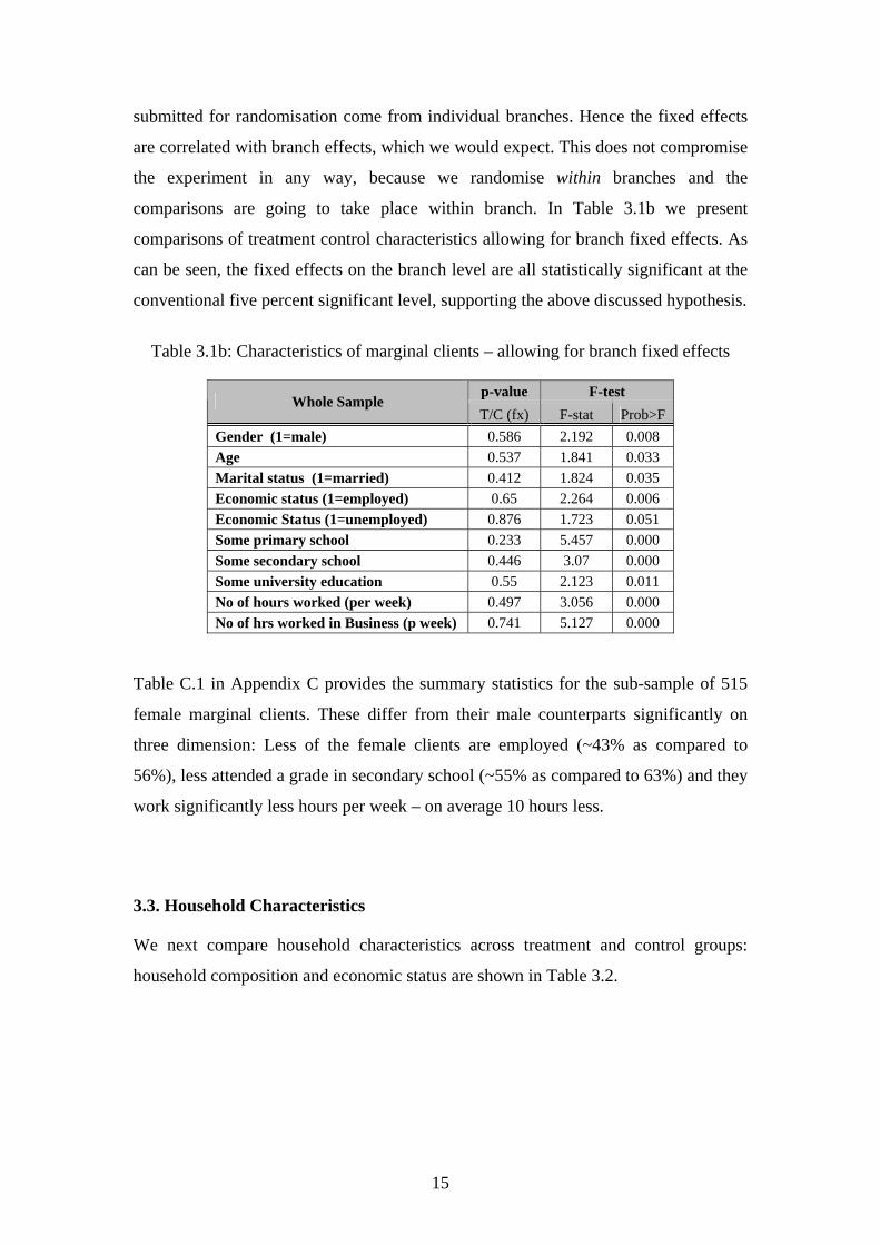
conventional five percent significant level, supporting the above discussed hypothesis.

Table 3.1b: Characteristics of marginal clients – allowing for branch fixed effects

p-value F-test Whole Sample

T/C (fx) F-stat Prob>F Gender (1=male) 0.586 2.192 0.008 Age 0.537 1.841 0.033 Marital status (1=married) 0.412 1.824 0.035 Economic status (1=employed) 0.65 2.264 0.006 Economic Status (1=unemployed) 0.876 1.723 0.051 Some primary school 0.233 5.457 0.000 Some secondary school 0.446 3.07 0.000 Some university education 0.55 2.123 0.011 No of hours worked (per week) 0.497 3.056 0.000 No of hrs worked in Business (p week) 0.741 5.127 0.000

Table C.1 in Appendix C provides the summary statistics for the sub-sample of 515

female marginal clients. These differ from their male counterparts significantly on

three dimension: Less of the female clients are employed (~43% as compared to

56%), less attended a grade in secondary school (~55% as compared to 63%) and they

work significantly less hours per week – on average 10 hours less.

3.3. Household Characteristics

We next compare household characteristics across treatment and control groups:

household composition and economic status are shown in Table 3.2.

16

Table 3.2: Characteristics of marginal clients’ households (1)

control (2)

treatment (3)

p-value (4)

p-value (5) (6)

F-test

(sd) (sd) T/C T/C (fx) F-stat Prob>F

3.43 3.58 # of hh members ( 1.43) ( 1.51)

0.061 0.076 1.005 0.471

1.73 1.89 # male household members ( 0.95) ( 1.07)

0.009 0.02 1.178 0.041

1.69 1.7 # female hh members ( 1.01) ( 0.97)

0.894 0.75 1.012 0.445

0.29 0.25 # kids age 0-5 ( 0.58) ( 0.54)

0.325 0.399 1.13 0.097

0.27 0.27 # kids age 6-10 ( 0.56) ( 0.56)

0.875 0.943 0.882 0.899

0.29 0.4 # kids 11-16 ( 0.58) ( 0.66)

0.002 0.004 0.976 0.591

0.18 0.14 # elders older than 63 ( 0.46) ( 0.39)

0.117 0.22 1.212 0.02

0.7 0.84 # hh members attending school ( 0.92) ( 0.98)

0.011 0.022 0.913 0.821

1.08 1.18 # employed hh members ( 0.93) ( 0.94)

0.06 0.071 1.203 0.024

0.72 0.69 # unemployed hh members ( 0.90) ( 0.91)

0.603 0.573 0.953 0.686

0.31 0.3 # retired hh members ( 0.52) ( 0.54)

0.685 0.836 1.072 0.23

0.33 0.38 # of female employed hh members ( 0.51) ( 0.56)

0.086 0.093 1.106 0.141

We see that the households consist on average of slightly more than 3 members. On

average a household consists of about 1.8 male and 1.7 female members. The number

of children is relatively equally distributed over the age ranges 0-5 year, 6-10 years

and 11-16 years, with approximately a third of a child in each age range. About 20 per

cent of all household members are over the age of 64.

We see two apparently significant differences (at the 5% level) between the treatment

and control group: Households that do get a loan have significantly more male

household members and more kids in the age range 11-16 years. In line with these,

treatment households also have more household members (0.84 as compared to 0.7

for control households) that are currently attending school.

17

There are no further significant differences between the two groups. Of course in a

series of tests over a large number of characteristics one expects some rejections (as

implied by the type 1 error).

Table 3.3 displays means and standard deviations for control and treatment household

members, looking at female adults aged 16 and over.

Table 3.3: Characteristics of all female adults 16+

Control treatment

(sd) (sd) Age 40.34 39.85* (16.07) (15.47) Married (0/1) 0.62 0.6 ( 0.48) ( 0.49) Employed (0/1) 0.26* 0.29* ( 0.44) ( 0.45) Unemployed (0/1) 0.26 0.23 ( 0.44) ( 0.42) Some primary school (0/1) 0.38* 0.43* ( 0.48) ( 0.50) Some secondary school (0/1) 0.53* 0.48* ( 0.50) ( 0.50) some university level (0/1) 0.10 0.09* ( 0.30) ( 0.29) Hrs work per week 24.13* 27.59* (26.54) (26.33) Hrs work in business per week 13.78 16.01 (22.10) (23.22) Stars indicate a significant difference between male and female respondents

Female adults in the sample are on average 40 years old and the majority (61%) are

married. About 30% have a job and about a quarter are unemployed. Half of them

have some secondary education and almost 10% went to university. They work on

average 25 hours a week, of which about 55% is spent on the household (or own)

business.

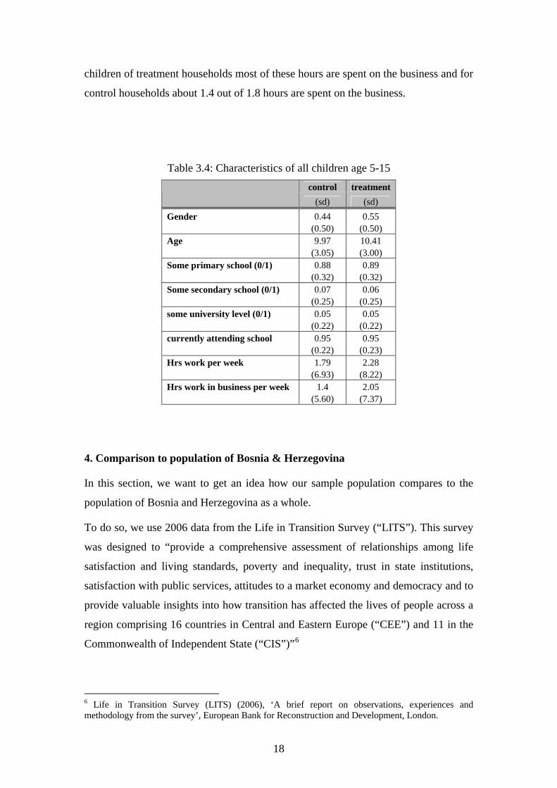
Finally, we take a look at age and education of children aged 5-15, displayed in Table

3.4. Most of these children are enrolled in primary school and about 7% in secondary

school. This implies that 95% of children in the analysed age range go to school. As

can be seen, they also do some work: About two hours per week on average. For

18

children of treatment households most of these hours are spent on the business and for

control households about 1.4 out of 1.8 hours are spent on the business.

Table 3.4: Characteristics of all children age 5-15

control treatment

(sd) (sd) Gender 0.44 0.55 (0.50) (0.50) Age 9.97 10.41 (3.05) (3.00) Some primary school (0/1) 0.88 0.89 (0.32) (0.32) Some secondary school (0/1) 0.07 0.06 (0.25) (0.25) some university level (0/1) 0.05 0.05 (0.22) (0.22) currently attending school 0.95 0.95 (0.22) (0.23) Hrs work per week 1.79 2.28 (6.93) (8.22) Hrs work in business per week 1.4 2.05 (5.60) (7.37)

4. Comparison to population of Bosnia & Herzegovina

In this section, we want to get an idea how our sample population compares to the

population of Bosnia and Herzegovina as a whole.

To do so, we use 2006 data from the Life in Transition Survey (“LITS”). This survey

was designed to “provide a comprehensive assessment of relationships among life

satisfaction and living standards, poverty and inequality, trust in state institutions,

satisfaction with public services, attitudes to a market economy and democracy and to

provide valuable insights into how transition has affected the lives of people across a

region comprising 16 countries in Central and Eastern Europe (“CEE”) and 11 in the

Commonwealth of Independent State (“CIS”)”6

6 Life in Transition Survey (LITS) (2006), ‘A brief report on observations, experiences and methodology from the survey’, European Bank for Reconstruction and Development, London.

19

For this survey, 1,000 households were interviewed in Bosnia and Herzegovina,

representative at a national level. Two respondents were sampled: The first one is the

household head or another household member with sufficient knowledge about the

household (roster and expenses) and the second sampled person (if different from the

first) is the person aged 18 years and over, who last had a birthday in the household.

4.1. Individual Characteristics

We will first compare our marginal clients to these two respondent types and then

concentrate on the ‘typical household member’ (the respondent who had last birthday

in the household as described above) as only limited information is available on the

household head.

As can be seen from Table 4.1a, the average marginal client is younger than the

representative respondent as well as household head in Bosnia and Herzegovina with

38 years as compared to 44 and 50 respectively.

60 percent of our marginal clients are male, which compares to 74 percent of

household heads being male in Bosnia and Herzegovina and 42% of the random

respondent.

Table 4.1a: Characteristics of respondents & household head

LITS SURVEY RESPONDENT

Obs Mean SD Min Max Obs Mean SD Min Max age respondent 1000 44.28 17.83 18 91 1205 37.61 12.25 17 70 age hh head 1000 50.32 15.58 18 91 gender respondent (male=1) 1000 0.42 0.49 0 1 1206 0.60 0.49 0 1 gender hh head (male=1) 1000 0.74 0.44 0 1

Table 4.1b displays educational characteristics and economic status of the marginal

client as compared to the respondent (not household head) from the LITS survey. It

can be seen that a higher percentage of the marginal clients has only compulsory

school education than the average adult person in Bosnia and Herzegovina (32% as

compared to 17%) and also more marginal clients have under the category of

“professional, vocational school/training” – 58% as compared to 44%. In line with

this, less marginal clients have secondary education or a higher professional degree.

20

Nevertheless, no one in our sample is totally uneducated, which compares to 14

percent of adult Bosnians not having attended school.

In terms of economic activity Table 4.1b shows that a much greater part of the

marginal clients is employed (57% as compared to 35%), which results from a smaller

number of marginal clients being students, retired or working in the house.

Table 4.1b: Characteristics of respondents

RESPONDENT (%) LITS Sample no degree/education 0.14 0.00 compulsory school education 0.17 0.32 secondary education 0.149 0.051 professional, vocational school/training 0.44 0.58

higher professional degree (university,…) 0.11 0.04

Education

post graduate degree 0.001 0.0008

employed 0.35 0.565 Unemployed/other 0.27 0.27 student 0.076 0.017 retired 0.16 0.093 housewife 0.14 0.057

Economic Status

child 0.0017

4.2. Household Characteristics

The average household size of marginal clients is slightly higher than the one of the

average household in Bosnia and Herzegovina with 3.5 as compared to 3.1 household

members. This additional household member is distributed relatively evenly among

age ranges of kids, while marginal clients have on average less household members

above the age of 63.

Table 4.2a: Household Characteristics LITS SURVEY

Household Composition Obs Mean SD Min Max Obs Mean SD Min Max

# household members 1000 3.09 1.47 1 9 1206 3.51 1.48 1 10 # male household members 1000 1.50 0.99 0 6 1206 1.82 1.02 0 6 # female household members 1000 1.59 0.94 0 5 1206 1.69 0.99 0 6 # kids 0-5 yrs 1000 0.17 0.45 0 3 1206 0.27 0.56 0 4 # kids 6-10 yrs 1000 0.15 0.41 0 2 1206 0.27 0.56 0 3 # kids 11-16 yrs 1000 0.22 0.53 0 3 1206 0.35 0.62 0 3 # elders (>=64 yrs) 1000 0.38 0.65 0 3 1206 0.16 0.42 0 2

21

Table 4.2b displays the different sources from which sample and LITS households

receive income.

Table 4.2b: Characteristics of respondents

LITS Sample

Household Income Sources Yes (%)

As main

source

Yes (%)

Income from wages (work for an employer) in cash 0.56 0.49 0.87

Wages in kind (e.g. products or services from the employer) 0.01 0.01 Income from self-employment, own or family business, or income from farm 0.21 0.10 0.78

Pensions 0.38 0.29 0.33 Investments, savings, rental of property (Apartment or plot of land) 0.01 0.00 0.04 State provided social benefits (inc unemployment benefits) 0.03 0.01 0.30 Help from relatives or friends including alimonies 0.12 0.05 0.21 Stipend income 0.01 Help from charities and non government organisations 0.00 Other sources 0.06 0.02 0.03

The two dominating income sources of marginal households are income from wages

as well as income from self-employment. They also receive a significant share from

pensions as well as other social benefits. Interestingly, 20% of our marginal client’s

households receive also help from friends or relatives. This latter percentage is almost

twice that of a typical household in Bosnia and Herzegovina. The other dominating

income sources are the same as those from our marginal clients: income from wages,

income from self-employment and pensions. Nevertheless, percentages are noticeably

lower (except for income from pensions). This holds – not surprisingly – especially

for income from self-employment: 78% of marginal clients get income from this

source, while only 21% of LITS households’ do.

Very comparable are the proportions of households in our and the LITs sample that

live in a house and that live in an apartment (Table 4.2c). For both samples, about

83% of households live in a house and 16% in an apartment. Of these, most are

owned - 89% of LITS households own the dwelling they live in and 87% of our

sample; and only few are rented – 17% and 16% for our two samples respectively.

22

Table 4.2c: Characteristics of dwelling

Dwelling (%) LITS Sample a house 82.9 83.42 an apartment 16.4 16.58 other 0.7 owned 89.90 87.31 rented 8.70 12.35 dk/na 1.40 0.33

Table 4.2d shows that also the percentages of households owning a second residence

are very comparable and lie at about 17%. The same holds for owning a car, which

54% of sampled households do.

Table 4.2d: Characteristics of assets

Assets (%) LITS Sample 2nd residence 17.95 17.49 car 54.25 54.31 mobile 68.9 95.94 computer 29.4 35.74

We observe that marginal clients relatively often own a mobile phone and a computer.

While this could be because more of the marginal households are self-employed, it is

more likely that the difference reflects the fact that the LITS data were collected in

2006, three years before our survey. As in other countries, Bosnia and Herzegovina

experienced an increase in ownership of technological appliances over recent years.

4.3. Poverty

In this section, we look at the poverty profile of the potential marginal clients. We are

interested in the poverty of the marginal clients compared to the overall population in

Bosnia and Herzegovina because this relates to the targeting of the loans. We

therefore make use of the 2007 Household Budget Survey (HBS) for Bosnia and

Herzegovina which was implemented in partnership by the Agency for Statistics of

Bosnia and Herzegovina, the Federal Office of Statistics and the Republika Srpska

Institute for Statistics.

In line with the HBS 2007 report on poverty and living conditions, we will

concentrate on poverty defined by a level of expenditure below a certain threshold.

Household consumption is used as a measure of material well-being - a first step for a

23

full comprehension of the main features of social exclusion, deprivation and economic

vulnerability.

To start with, expenditure thresholds that define poverty need to be defined and with

these we can then analyse the resulting poverty rates of our marginal clients. We will

compare expenditures of our sample to poverty lines constructed in the HBS report –

a pure food poverty line as well as a general poverty line.

Before doing so, we want to get a feeling of how our sample compares to the overall

population in terms of their consumption expenditures. Table 4.3 shows the

distribution of total yearly household consumption derived through the 2007

Household Budget Survey.

Table 4.3: Distribution of total household consumption

Source: HBS 2007 – poverty and living conditions, p. 12

As will be seen in section 5.1 below, the average total yearly consumption

expenditure of the marginal clients’ households is KM 10,000 with a standard

deviation of about KM 8,400. Adjusting for inflation in 2008 using the inflation rate

of 7.4% as published by the International Monetary Fund, this translates into KM

9,926. The potential marginal clients seem to fall into approximately the third quintile

of the population in terms of their expenditure patterns. This is a sensible finding

given that a microfinance institution aims at serving the poorer strata of the

population but usually leaves out the very poor due to too high risks.

To construct the poverty line the HBS 2007 report spatially deflates the consumption

expenditure data and expresses it in per capita terms. The former is done since

geographic differences in prices can cause the same bundle of goods to be more

24

expensive in one region than in another but this difference does not reflect differences

in material well-being and hence needs to be accounted for. Since a full-fledged

poverty analysis is beyond the scope of this report, we will not adjust our data for

regional price differences. Nevertheless, we are quite confident that we can get a

reasonable estimate of the poverty status of our sample. Comparing the per capita

consumption expenditure of our sample households to spatially adjusted results of the

HBS 2007 survey (displayed in Table 4.4), we still find that the marginal clients fall

approximately into the third decile of the population. Adjusted for inflation, per capita

expenditure in our sample is KM 3,486.

Table 4.4: Distribution total per capita consumption expenditure (adjusted for spatial price differences)

Source: HBS 2007 – poverty and living conditions, p. 13

Food Poverty

To construct the food poverty line, the HBS 2007 report starts with determining the

consumption patterns of a representative subset of the population. Their suggested

choice is aligned with the World Bank Poverty Assessment of 2003 who chooses the

second and third deciles of the population (in the distribution of consumption

expenditures), “because our interest is in people at the lower end of the distribution”

(WB (2003, p. 33)). “The poorest decile of the population is excluded as the

consumption patterns of those people might not be representative of a normal pattern

and they may reflect measurement errors.”

25

According to their calculations, the cost of a minimum-calories food bundle for the

reference group in 2007 is equal to KM 1,005.68. This is the average 2007 food

poverty line for Bosnia and Herzegovina. Using the CPI for food and non-alcoholic

beverages published by the Statistical Office of Bosnia and Herzegovina, which

averages at 11.925 for 2008, this corresponds to a food poverty line of KM 1126

(1080) in 2008.

Of our sample, 40.6% spend less than the calculated threshold on food and beverages.

This compares to 21.37% of the overall population in 2007. This difference and high

percentage of food-poor in our sample is not surprising given that the marginal clients

fall into the third expenditure decile on average and that the second and third decile

was chosen to construct the poverty line reference group.

In terms of total consumption expenditure lying below the food poverty line, we find

this to be the case for 16.8% of the marginal clients’ households while it is only the

case for 0.52% of the overall population in 2007.

General Poverty Line

The general poverty line takes into account that food is not the only essential need,

but that money has to be spent on other items as well. The HBS 2007 report

constructs a general poverty line by “using per capita total consumption, adjusted for

spatial deflation, and considering as food consumption the total expenditure in those

food and beverage items (109) out of which the minimum food basket has been

calculated (with a selection of the 66 items listed in the WB (2003) poverty

assessment) considering the expenditure weights of the reference group only (the third

and second deciles of population per capita total consumption)” (p.21).

Doing so, the estimate of the general food poverty line is KM 3,154 in 2007. By

furthermore excluding health care expenditure (a category we do not include in our

consumption expenditure variable) and including meals outside home, the general

food poverty line becomes KM 2,857 in 2007. Adjusting for food inflation, it

becomes KM 3,198 in 2008.

The HBS 2007 report finds that 18.6 of the population in Bosnia and Herzegovina has

expenditures below this threshold. For the general poverty line, we find an even

greater difference between poverty in the country and in our sample. About 62% of

26

marginal clients fall under the general poverty line constructed as described above.

Interestingly, while for the overall population general poverty is less than food

poverty, we find in our sample a higher percentage of general poverty than food

poverty.

Table 4.5 displays a summary of the above discussed results and also presents further

poverty measures. For one, we look at the poverty gap ratio, or the amount of money

necessary to bring everyone in poverty right up to the poverty line, as a proportion of

the poverty line and averaged over the population. And second, results for the squared

poverty gap. This measure gives more weight to observations further away from the

poverty line, hence capturing the severity of poverty.

Table 4.5: Poverty Measures

HBS 2007 Our data food 0.214 0.402 Poverty Headcount general 0.186 0.605 food n.a. 0.158 Poverty Gap ratio general 0.049 0.285 food n.a. 0.088 Squared poverty gap general 0.019 0.167

It can be seen that both, poverty depth (poverty gap ratio) as well as severity (squared

poverty gap) is much higher for our sample population than for the population of

Bosnia and Herzegovina as a whole.

5. Socio-economic household indicators

Having compared our sample households to a representative sample of the population

in Bosnia and Herzegovina, this section will now describe our sample households in

more detail, looking at consumption expenditures, assets, income, savings and shocks

the household experienced. The next section will then concentrate on the households

business(es), loans and the EKI loan the household applied for in particular.

5. 1. Household consumption

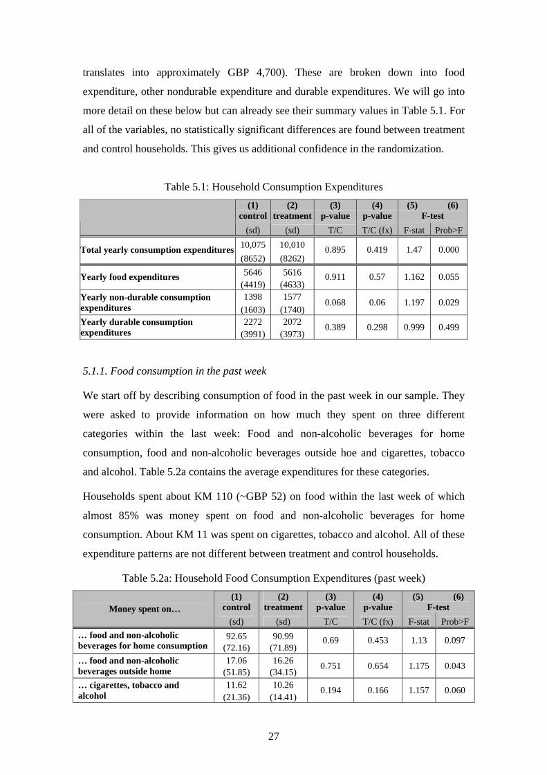
Table 5.1 shows statistics for aggregate consumption variables. Sample households

spent on average KM 10,000 within the last year on different expenditure items (this

27

translates into approximately GBP 4,700). These are broken down into food

expenditure, other nondurable expenditure and durable expenditures. We will go into

more detail on these below but can already see their summary values in Table 5.1. For

all of the variables, no statistically significant differences are found between treatment

and control households. This gives us additional confidence in the randomization.

Table 5.1: Household Consumption Expenditures (1)

control(2)

treatment(3)

p-value (4)

p-value (5) (6)

F-test (sd) (sd) T/C T/C (fx) F-stat Prob>F

10,075 10,010 Total yearly consumption expenditures(8652) (8262)

0.895 0.419 1.47 0.000

5646 5616 Yearly food expenditures (4419) (4633)

0.911 0.57 1.162 0.055

1398 1577 Yearly non-durable consumption expenditures (1603) (1740)

0.068 0.06 1.197 0.029

2272 2072 Yearly durable consumption expenditures (3991) (3973)

0.389 0.298 0.999 0.499

5.1.1. Food consumption in the past week

We start off by describing consumption of food in the past week in our sample. They

were asked to provide information on how much they spent on three different

categories within the last week: Food and non-alcoholic beverages for home

consumption, food and non-alcoholic beverages outside hoe and cigarettes, tobacco

and alcohol. Table 5.2a contains the average expenditures for these categories.

Households spent about KM 110 (~GBP 52) on food within the last week of which

almost 85% was money spent on food and non-alcoholic beverages for home

consumption. About KM 11 was spent on cigarettes, tobacco and alcohol. All of these

expenditure patterns are not different between treatment and control households.

Table 5.2a: Household Food Consumption Expenditures (past week) (1)

control (2)

treatment (3)

p-value (4)

p-value (5) (6)

F-test Money spent on… (sd) (sd) T/C T/C (fx) F-stat Prob>F

92.65 90.99 … food and non-alcoholic beverages for home consumption (72.16) (71.89)

0.69 0.453 1.13 0.097

17.06 16.26 … food and non-alcoholic beverages outside home (51.85) (34.15)

0.751 0.654 1.175 0.043

11.62 10.26 … cigarettes, tobacco and alcohol (21.36) (14.41)

0.194 0.166 1.157 0.060

28

5.1.2. Consumption of other non-durables in the past month

Next, we look at consumption expenditures on other non-durable items (Table 5.2b).

This table differs from the previous ones as we now also show the means and standard

deviations conditional on having spent money on a certain item (columns (7) and (8)).

As some households did not purchase some of the goods, the averages displayed in

columns (1) and (2) give a slightly wrong picture on how much a household actually

spent, if it spent money on it, which can be better understood from the conditional

means. To get additionally an understanding on how many households did not have

any expenditures for a certain item, we display the number of such households in

columns (9) and (10).

For the whole sample we can see that within the last month, most money was spent on

combustibles. This would be fuel for the stove, fuel for heating, gas, and petrol. This

is the only variable in all our expenditure items for which we find a significant

difference between our control and treatment groups, with treatment households

having spent KM 67 and control households KM 52. All other expenditure categories

are comparable between the two groups.

Table 5.2 Household other non-durables consumption expenditures (past month)

Whole sample Conditional on having spent money (1)

control (2)

treatment (3)

p-val (4)

p-val (5) (6)

F-test (7)

contr. (8)

treatm. (9)

contr. (10)

treatm. Item

(sd) (sd) T/C T/C (fx)

F-stat Prob>F (sd) (sd) # zeros # zeros

12.17 8.18 147.38 133.15 rent (49.25) (34.54)

0.101 0.229 1.582 0.000 (97.91) (53.18)

522 596

51.80 66.60 105.84 133.41 combustibles (96.10) (121.34)

0.02 0.03 1.187 0.034 (114.73) (143.53)

289 318

14.76 15.38 48.01 52.66 transport (34.62) (61.40)

0.834 0.761 2.505 0.000 (48.03) (104.81)

394 451

34.78 42.36 97.16 100.21 clothes and shoes (78.59) (69.84)

0.077 0.113 1.16 0.058 (105.91) (75.79)

364 366

3.16 2.46 51.26 35.61 recreation (27.53) (12.21)

0.562 0.547 1.539 0.000 (100.51) (31.58)

533 593

7.09 5.03 19.5 15.04 magazines (28.07) (13.13)

0.096 0.119 0.8 0.988 (43.93) (19.13)

362 424

6.64 4.31 198.74 114.38 fee, insurance (66.62) (29.32)

0.424 0.364 0.752 0.998 (315.83) (103.15)

550 613

0.36 3.82 51.5 242.8 remittances ( 6.52) (65.06)

0.207 0.236 0.612 1.000 (67.40) (483.42)

565 625

29

The right block of Table 5.2hows that the greatest amount of money was spent on rent

as well as fees and insurance, closely followed by combustibles and clothes and

shoes. For most of these, many households did not spend any money though. For

example rent was only paid by 47 control and 41 treatment households.

5.1.3. Consumption of other durables in the past year

The third consumption expenditure category is durable items and households were

asked how much they spent on these within the last year. Results are presented in

Table 5.2c, which follows the format of the previous table.

Again, none of the variables are significantly different in their means between the two

groups. On average, most money was spent on repairs and only very little on

vacation. When considering conditional means we see that the biggest chunk on

money was spent on buying a car and repairs still make up an important part of

expenditures.

Table 5.2c Household durable consumption expenditures (past year)

Whole sample Conditional on having spent money (1)

control (2)

treatment (3)

p-val (4)

p-val (5) (6)

F-test (7)

control (8)

treatmnt (9)

control (10)

treatmnt Item

(sd) (sd) T/C T/C (fx)

F-stat Prob>F (sd) (sd) # zeros # zeros

315.7 263.6 726.3 536.5 Education (841.9) (710.8)

0.246 0.42 0.585 1.000 (1156) (939.7)

320 321

374 360.7 1047 1197 Furniture (910.0) (985.6)

0.807 0.664 0.878 0.907 (1272) (1493)

365 445

1002.91 954.1 2438 2443 Repairs (3364) (3309)

0.8 0.383 1.241 0.011 (4906) (4946)

335 387

178.7 175.7 639.5 589.1 Household appliances (1028) (792.3)

0.955 0.343 5.672 0.000 (1872) (1367)

410 447

550.1 509.5 3639.9 3567 purchase of vehicle (2192) (2056)

0.74 0.663 0.813 0.982 (4551) (4341)

483 546

13.56 16.36 593.62 694.7 vacation (122.6) (175.5)

0.751 0.727 0.684 1.000 (582) (945.4)

556 622

5.2. Household assets

Table 5.3a shows that the household of a marginal client owns assets with a current

market value of approximately KM 125-130,000 (~GBP 60,000), including the value

of their house and land.

30

Table 5.3a: Household asset value, total

control treatment p-value p-value F-test (sd) (sd) T/C T/C (fx) F-stat Prob>F

125,773 131,466 Asset value, total (128,422) (170,163)

0.559 0.559 1.062 0.271

Table D.1 in Appendix D gives the statistics for the different items the aggregate in

Table 5.3a is made up of. From the value of ownership owned houses/dwellings (first

item in Table D.1) we can learn that the value of this property is approximately KM

85,000 (~GBP 40,000).7 From Section 4.2 (Table 4.2c) we know that about 84% of

the interviewed households own the place they live in.

The last things we will look at with respect to household assets are a few variables

relating to the dwelling of the household. These are displayed in Table D.1 in

Appendix D. Most households live in a house which they own and this does not differ

between the control and the treatment group. Also, the size of their dwelling is on

average the same, lying at about 110 square meters. The only significant difference

we find is in the ownership of a second property – 23% (131 households) of control

households do so as compared to only 16% (104 households) of treatment households.

Table 5.3b: Household asset, ownership (1)

control (2)

treatment (3)

p-value (4)

p-value (5) (6)

F-test (sd) (sd) T/C T/C (fx) F-stat Prob>F

0.83 0.83 Dwelling: house (%) (0.3733) (0.3716)

0.9308 0.6312 1.0513 0.295

0.17 0.17 Dwelling: apartment (%) (0.3733) (0.3716)

0.9308 0.6312 1.0513 0.295

0.86 0.89 Dwelling: owned (%) (0.35) (0.32)

0.179 0.216 1.161 0.056

0.14 0.11 Dwelling: rented (%) (0.34) (0.32)

0.181 0.209 1.188 0.034

106 111 Square meters of dwelling (82.33) (123.79)

0.495 0.546 2.813 0.000

0.23 0.16 Any other dwellings owned (%) (0.42) (0.37)

0.003 0.007 0.984 0.559

7 Note that the value of own property is slightly lower as households own on average 1.07 houses.

31

5.3. Household income

As in the previous section, we will also proceed in this section on household income

by looking at the aggregate household income and then the different income sources.

Households earn approximately KM 18,000 in a year (~GBP 8,500) – again, no

significant differences in these means between our two groups.

Table 5.4a: Household income, total (1)

control (2)

treatment (3)

p-value (4)

p-value (5) (6)

F-test (sd) (sd) T/C T/C (fx) F-stat Prob>F

18,183 17,397 Total Yearly household income (16,024) (12,477)

0.34 0.577 1.62 0.000

It is interesting to see how this income compares to expenditures. Table 5.4b shows

that control households earn slightly less than they spent and the opposite holds for

treatment households. Note though that this difference is not statistically significant.8

Table 5.4b: Household income minus household expenditures (1)

control (2)

treatment (3)

p-value (4)

p-value (5) (6)

F-test (sd) (sd) T/C T/C (fx) F-stat Prob>F

456.39 -614.01 Total income minus expenditures (54401) (56696)

0.739 0.812 0.862 0.933

As already pointed out in section 4.2., when comparing marginal client households to

the LITS sample, almost 80% of our households have income from self-employment.

This is not surprising given that a member of these households applies for a loan with

EKI, most of which are meant for investment in business (see section 6.3 for more

details on this). About half of the sample receives income from wages from private

businesses other than their own. Other important income sources are pensions and

other social benefits as well as wages from government and manufacturing. No

significant differences in means between groups can be detected. More details on the

percentages of household earning income from a given source are displayed in

Appendix D, Table D.2.

8 Means of total consumption displayed in Table 7 exclude observations with extreme expenditures, which lowers the average and because of which it seems as if households should all be able to save when comparing to means of household income in Table 10a.

32

These same income sources are listed in Table 5.4c. Additionally, this table gives

information on the amount households earn from the respective sources –

unconditional and conditional means are presented. Households receive highest

returns from their own enterprise as well as from work in the financial sector and

wages from the government – all of these income sources earn an approximate yearly

income of KM 10,000 (~GBP 4,700). Income sources with lowest returns are benefits

from the government (other than pensions) and remittances, closely followed by

wages from agricultural work and income from rental properties.

Table 5.4c: ANNUAL Household income, amount per source

Whole sample Conditional on earning income (1)

control (2)

treatment (3)

p-val (4)

p-val (5) (6)

F-test (7)

contr. (8)

treatm. (9)

contr. (10)

treatm. Income Source

(sd) (sd) T/C T/C (fx) F-stat Prob>F (sd) (sd) # zeros # zeros

8052 7189 10319 9236 Self-employment (14607) (9612)

0.221 0.568 1.714 0.000 (15815) (9991)

125 141

330 296 3025 2769 Wages from Agric. Work (1421) (1227)

0.66 0.502 0.83 0.970 (3242) (2707)

507 568

295 330 5990 5374 Wages from shop/market work (1435) (1490)

0.681 0.647 0.526 1.000 (2813) (3047)

541 597

56 107 10633 16950 Wages: work in bank/financ. services (798) (1769)

0.531 0.534 0.605 1.000 (3493) (16776)

566 632

559 621 7396 9188 Wages: manufacturing industry (2241) (2897)

0.679 0.539 0.886 0.890 (4017) (6805)

526 593

30 2 5667 1200 Wages: tourism (468) (48)

0.134 0.163 0.413 1.000 (3786)

566 635

4579 4798 9371 9844 Wages: other private business (6882) (7318)

0.593 0.822 1.037 0.348 (7214) (7759)

291 326

1368 1291 10381 10806 Wages: government (4522) (4124)

0.757 0.43 1.011 0.448 (7884) (6311)

494 560

426 357 2056 1680 Migration income / remittances (1302) (1042)

0.302 0.21 0.756 0.998 (2201) (1706)

451 501

602 554 2089 1736 Benefits from government (1354) (1153)

0.507 0.68 1.198 0.027 (1806) (1456)

405 433

1695 1538 5022 4865 Pensions (3360) (3657)

0.44 0.783 0.847 0.954 (4094) (5118)

377 435

97 190 3064 4477 Income from rental properties (766) (1706)

0.231 0.306 0.851 0.948 (3159) (7155)

551 609

95 125 4509 3793 Other income sources (1117) (1329)

0.672 0.673 0.554 1.000 (6539) (6441)

557 615

5.4. Household Savings

We already got a first impression on household income net of expenditures from

Table 10b and could see that their potential for savings is not extensive. Here, we

33

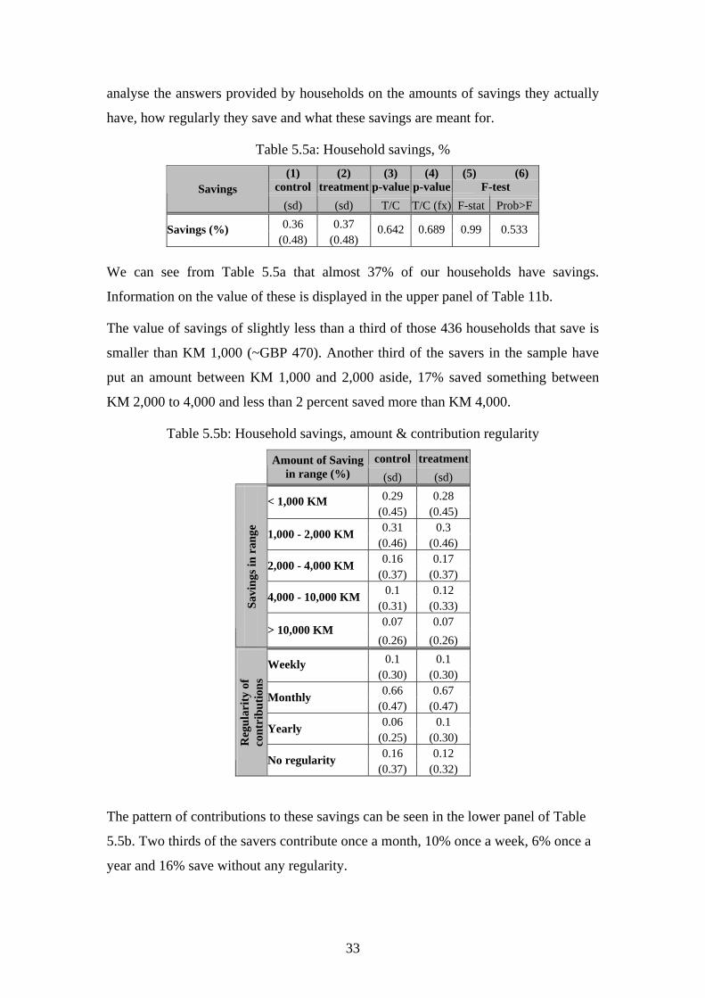
analyse the answers provided by households on the amounts of savings they actually

have, how regularly they save and what these savings are meant for.

Table 5.5a: Household savings, % (1)

control (2)

treatment(3)

p-value(4)

p-value(5) (6)

F-test Savings (sd) (sd) T/C T/C (fx) F-stat Prob>F 0.36 0.37 Savings (%)

(0.48) (0.48) 0.642 0.689 0.99 0.533

We can see from Table 5.5a that almost 37% of our households have savings.

Information on the value of these is displayed in the upper panel of Table 11b.

The value of savings of slightly less than a third of those 436 households that save is

smaller than KM 1,000 (~GBP 470). Another third of the savers in the sample have

put an amount between KM 1,000 and 2,000 aside, 17% saved something between

KM 2,000 to 4,000 and less than 2 percent saved more than KM 4,000.

Table 5.5b: Household savings, amount & contribution regularity

control treatment

Amount of Saving in range (%) (sd) (sd)

0.29 0.28 < 1,000 KM (0.45) (0.45) 0.31 0.3 1,000 - 2,000 KM

(0.46) (0.46) 0.16 0.17 2,000 - 4,000 KM

(0.37) (0.37) 0.1 0.12 4,000 - 10,000 KM

(0.31) (0.33) 0.07 0.07

Savi

ngs i

n ra

nge

> 10,000 KM (0.26) (0.26)

0.1 0.1 Weekly (0.30) (0.30) 0.66 0.67 Monthly

(0.47) (0.47) 0.06 0.1 Yearly

(0.25) (0.30) 0.16 0.12

Reg

ular

ity o

f co

ntri

butio

ns

No regularity (0.37) (0.32)

The pattern of contributions to these savings can be seen in the lower panel of Table

5.5b. Two thirds of the savers contribute once a month, 10% once a week, 6% once a

year and 16% save without any regularity.

34

The greatest motivation for savings is stated to be consumption smoothing –two thirds

of all households that save do so to be prepared for emergency events or to secure

consumption specifically (36% of all saving households name this as their primary

reason to save and an additional 4% states securing consumption specifically as their

primary reason). These statistics are displayed in Table D.3 in Appendix D. Other

important motivations to save are future business expenses and education, medical

expenses and provision for old age. Paying for debt is not mentioned by any

household as a reason for saving.

5.5. Shocks experienced by the households

We now turn to shocks the households experienced over the last year. These are

mainly negative shocks but we also consider shocks that could result in an income

gain to households.

The number of negative and positive shocks experienced is summarized in Table 5.6a.

About half of the sample experienced one negative shock and households experienced

on average only 0.03 positive shocks. Resulting from the negative shocks, about 20%

of all households experienced an income loss. No significant differences are found

between treatment and control households.

Table 5.6a: Number of shocks experienced

Whole sample (1)

control (2)

treatment (3)

p-value (4)

p-value (5) (6)

F-test Shock experienced

(sd) (sd) T/C T/C (fx) F-stat Prob>F

0.54 0.53 No of negative shocks experienced in the last year ( 0.76) ( 0.73)

0.77 0.783 1.169 0.049

0.03 0.03 No of positive shocks experienced in the last year (0.17) (0.18)

0.645 0.527 1.354 0.001

0.23 0.19 Income loss experienced in last year (0.42) (0.40)

0.085 0.117 1.017 0.424

35

Table 5.6b gives more details on the type of shocks experienced.

Table 5.6b: Type of shocks and income reduction experienced, %

Whole sample Imcome reduction due to shock

(conditional on having experienced the shock)

(1) control

(2) treatment

(3) p-val

(4) p-val

(5) (6) F-test

(7) contr.

(8) treatm.

(9) contr.

(10) treatm.

Shock experienced (%)

(sd) (sd) T/C T/C (fx) F-stat Prob>F (sd) (sd)

# zeros # zeros

0.09 0.07 0.69 0.62 Household member lost job ( 0.28) ( 0.26)

0.321 0.346 0.965 0.637 (0.47) (0.49)

15 17

0.05 0.06 0.73 0.68 Bad harvest ( 0.22) ( 0.23)

0.68 0.624 1.18 0.039 (0.45) (0.47)

8 12

0.07 0.07 0.59 0.55 Illness of earning household member ( 0.26) ( 0.25)

0.681 0.727 1.017 0.425 (0.50) (0.50)

17 19

0.06 0.07 0.53 0.40 Illness of non-earning household member ( 0.24) ( 0.26)

0.605 0.325 1.419 0.000 (0.51) (0.50)

17 27

0.02 0.02 0.78 0.67 Death of earning household member ( 0.12) ( 0.15)

0.336 0.336 0.884 0.895 (0.44) (0.49)

2 5

0.03 0.01 0.53 0.33 Death of non-earning household member ( 0.17) ( 0.12)

0.061 0.037 0.937 0.743 (0.51) (0.50)

8 6

0.01 0.02 0.67 0.80 Criminal/Corruption against business ( 0.10) ( 0.12)

0.433 0.268 0.983 0.564 (0.52) (0.42)

2 2

0.17 0.17 0.34 0.31 Increased market competition ( 0.38) ( 0.37)

0.741 0.597 1.119 0.116 (0.48) (0.47)

65 72

0.02 0.03 0.08 0.00 Household member FOUND job outside own business ( 0.15) ( 0.16)

0.794 0.653 1.405 0.000 (0.28) (0.00)

12 16

For the sample as a whole, the most common shock was increased market

competition, which 17% of households named. Other prevalent shocks are the loss of

a job by a household member and the falling ill of an earning household member.

In terms of positive shocks, we learn that only 2-3 percent of all households

underwent such a shock, which is more specifically that a household member found a

job outside the household business.

Note that the right block of Table 5.6b is as before conditional on having experienced

a certain shock, but the information provided is actually whether the household

experienced a loss in their income due to having experienced the given shock.

So, for example 70% of those control households who had a member loosing its job

within the last year actually experience a household income reduction due to this loss.

The other 40% most likely managed to find an alternative income source relatively

quickly.

36

6. Household business and loans

6.1. Household business

Table 6.1a shows that 63% of all loan applicants already own a business. This

proportion is exactly the same for the control and the treatment group. This translates

into 765 of our 1206 interviewed households being business owners – 404 in the

treatment group and 361 in the control group. Of these businesses, 12% of the

treatment and 11% of the control group are registered.

Table 6.1a: Owning a business, % (1)

control (2)

treatment (3)

p-value (4)

p-value (5) (6)

F-test Business owner (%) (sd) (sd) T/C T/C (fx) F-stat Prob>F 0.63 0.63 Business Owner (%)

(0.48) (0.48) 0.994 0.878 1.098 0.159

Out of the 765 households that own a business, 108 (so 9% of the overall sample and

14% of the business owners) additionally own a second business – 62 treatment

households and 46 control households.

In the remainder of this section we concentrate on those households that actually own

a business, or two. Table 6.1b displays several characteristics of these businesses,

again providing information for our treatment and our control group separately.

Almost all main businesses (left block of table 6.1b) are more or less equally

distributed among trade, services and agriculture/farming, the latter one the

dominating engagement with about 38% of our household’s businesses engaged in

this sector. About 5% of businesses are engaged in production. We find a somewhat

similar pattern for the secondary business, with slightly less involvement in trade but

more in services. Both, primary and secondary businesses have been in existence for

on average almost 10 years.

37

Table 6.1b: Characteristics of the main and the secondary business, %

Main Business (765 obs) 2nd Business (108 obs) control treatment control treatment control treatment control treatment (sd) (sd) # zeros # zeros (sd) (sd) # zeros # zeros

0.29 0.25 0.15 0.18 …trade (0.46) (0.43)

255 302 (0.36) (0.39)

39 51

0.28 0.30 0.37 0.37 …services (0.45) (0.46)

259 281 (0.49) (0.49)

29 39

0.36 0.39 0.39 0.37 …agriculture / farming (0.48) (0.49)

231 247 (0.49) (0.49)

28 39

0.06 0.05 0.09 0.08 Bus

ines

s eng

aged

in…

…production (0.24) (0.23)

338 382 (0.28) (0.27)

42 57

9.64 11.75 9.93 10.13 Years in existence (11.00) (15.02)

18 14 (7.95) (8.88)

1 2

0.98 1.00 0.48 0.76 …full-time (0.85) (0.87)

107 115 (0.59) (0.97)

26 32

0.62 0.61 0.96 0.68 …part-time (0.83) (0.81)

198 233 (0.92) (0.78)

16 31

0.28 0.26 0.33 0.19 No.

of h

h m

emb.

w

orki

ng…

…temporary (0.65) (0.66)

291 335 (0.76) (0.40)

37 50

990 887 956 528 Total monthly compensation hh members ( 1518) ( 1091)

12 5 ( 1639) ( 610)

1 2

10.48 1.49 5.65 6.60 …full-time (82.17) (24.88)

316 358 (36.84) (50.79)

42 57

0.07 0.07 0.00 0.05 …part-time (0.41) (0.54)

348 392 (0.00) (0.28)

46 60

0.29 0.22 1.00 0.89 No.

of o

utsi

ders

w

orki

ng…

…temporary (1.81) (0.81)

331 362 (5.89) (6.35)

40 57

249 214 513 37 Total monthly compensation outsiders (866.6) (726.5)

289 317 (2416.3) ( 143.6)

38 54

The next panel in the same table provides us information on employees within the

businesses. The main business has about one household member working full-time in

the enterprise, 0.6 member(s) part time and 0.3 on a temporary basis. The average

total monthly compensation for these workers is ~KM 950. For the secondary

business, more members work part-time and less full-time. The number of households

working in the business temporarily is comparable and so is the total monthly

compensation for secondary business of control households – it lies lower (at KM 530

for secondary businesses of treatment households).

38

The number of outsiders working part-time in the main business is negligible. Most

employees work full-time. We find a great difference for treatment and control

businesses with those of control households having ten employees more on average.

This discrepancy in number of outsiders working in the business full-time comes from

the fact that we have 3 businesses with 500 outsiders employed full time, 2 with 600

and 1 with 1,000 in the control group and only 1 business with 500 outsider employed

full-time. All other businesses have less than ten outsiders employed full-time.

The secondary businesses have on average six outsiders working full-time and one on

a temporary basis.

The average monthly compensation lies just above KM 200 for the main business and

500 for the secondary for controls and 40 for treatment household’s businesses.

With an overview of what type of businesses the marginal clients run, we now look at

their business revenues and expenditures, displayed in Table 6.1c.

Respondents were asked whether they prefer to talk about these variables in monthly

or yearly terms and their preference is reported in the first lines of the table (64%

preferring to think about them in monthly terms) but all values are converted into

yearly figures for ease of comparison.

We can see that for the main business, expenses are about KM 7,500 (~GBP 3,500),

revenues KM 18,000 (~GBP 8,500) so that the main business makes an average

yearly profit of KM 10,800 (~GBP 5,100).

Table 6.1c: Expenses and Revenues of the main and the secondary business, %

Main Business (765 obs) 2nd Business (108 obs) control treatment control treatment control treatment control treatment (sd) (sd) (sd) (sd) (sd) (sd) (sd) (sd)

0.63 0.64 0.52 0.55 Thinks about its profits in monthly terms (%) (0.48) (0.48)

135 145 (0.51) (0.50)

22 28

7,928 6,619 2,928 1,822 Expenses (yearly) (30,289) (16,030)

34 28 ( 7,278) ( 2,900)

7 18

19,109 17,218 8,547 7,357 Revenue (yearly) (41360) (29,818)

0 1 (14,123) ( 7,690)

0 0

10,914 10,639 5,619 5,535 Net profit (yearly) (19826) (19,203)

0 1 ( 7,319) ( 6,478)

1 0

39

For the secondary business, expenses are about KM 2,500 (~GBP 1,200), revenues

are approximately KM 8,000 (~GBP 3,700), which results in a business profit of

about KM 5,600 (~GBP 2,600).

6.1.1. Expected business profits

We asked those respondents who said that they would use the loan on an enterprise, to

state how much net profit they would expect to make over the next year if the

enterprise turned out to be extremely successful, and if it turned out to be extremely

unsuccessful. Statistics for these are shown in Table 6.1d below. The average

expected yearly profit in the case of a very successful enterprise is on average 61,000

Convertible Mark, whilst that of a very unsuccessful enterprise is about 30,000

Convertible Mark. Comparing these figures to actual net profits (repeated in the same

table for ease of comparison and graphed in Figure 6.1) and assuming the

expectations are provided in real terms, suggests that respondents are very optimistic

about the future – and such optimism is equally prevalent for the treatment and

control groups. Table 6.1e shows that there are no significant differences in

expectations between the two groups. It does not come at a surprise that respondents

are optimistic about their future business profit considering that we are dealing with a

sample of individuals that went to a microfinance institution to apply for a business

loan. It is safe to assume that most of these applicants are motivated people that

believe the situation to be right for expansion of their business or even setting-up of a

new one. This finding is in line with Augsburg (2009, p.12) who analyses the effect of

investment in India and argues that “The fact that clients made the decision to borrow

money from the institution and to invest it into a risky asset shows that the hope of

success is one of their characteristics. Independently of their degree of risk aversion,

they are most likely optimistic about one or several things, including for example

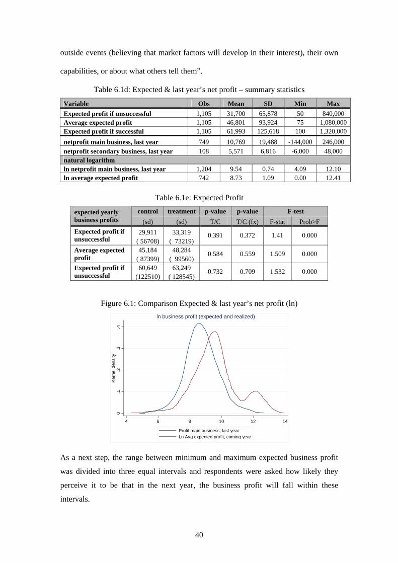
40

outside events (believing that market factors will develop in their interest), their own

capabilities, or about what others tell them”.

Table 6.1d: Expected & last year’s net profit – summary statistics

Variable Obs Mean SD Min Max Expected profit if unsuccessful 1,105 31,700 65,878 50 840,000 Average expected profit 1,105 46,801 93,924 75 1,080,000 Expected profit if successful 1,105 61,993 125,618 100 1,320,000 netprofit main business, last year 749 10,769 19,488 -144,000 246,000 netprofit secondary business, last year 108 5,571 6,816 -6,000 48,000 natural logarithm ln netprofit main business, last year 1,204 9.54 0.74 4.09 12.10 ln average expected profit 742 8.73 1.09 0.00 12.41

Table 6.1e: Expected Profit

control treatment p-value p-value F-test expected yearly business profits (sd) (sd) T/C T/C (fx) F-stat Prob>F

29,911 33,319 Expected profit if unsuccessful ( 56708) ( 73219)

0.391 0.372 1.41 0.000

45,184 48,284 Average expected profit ( 87399) ( 99560)

0.584 0.559 1.509 0.000

60,649 63,249 Expected profit if unsuccessful (122510) ( 128545)

0.732 0.709 1.532 0.000

Figure 6.1: Comparison Expected & last year’s net profit (ln)

0.1

.2.3

.4K

erne

l den

sity

4 6 8 10 12 14

Profit main business, last yearLn Avg expected profit, coming year

ln business profit (expected and realized)

As a next step, the range between minimum and maximum expected business profit

was divided into three equal intervals and respondents were asked how likely they

perceive it to be that in the next year, the business profit will fall within these

intervals.

41

We are interested how many respondents allocated a probability of zero or 100 to a

certain interval since that indicates that the range between minimum and maximum

expected profit might not reflect the true beliefs of the marginal clients. After all, if

they believe that the likelihood of profit falling in the first interval is zero, this might

imply that the minimum expected profit was stated too low. Table 6.13f shows that

respondents allocate zero to a number of intervals but that the amount of 100%

probability is even more worrisome: in case of the first interval, 44% of marginal

clients were 100% certain that their profit in the coming year would fall within this

interval – which would imply the maximum expected profit to be significantly

overestimated.

Table 6.1f: Expected Profit

Variable Obs Mean SD Min Max # 0 # 100 exp_proba 1,060 84 21 0 100 2 468 exp_probb 1,055 69 25 0 100 6 204 exp_probc 1,053 68 25 0 100 3 190 probA + probB + probC 1,052 222 63 0 300

Another interpretation is that the respondent did not understand the idea of the

probability that their profit falls within a certain interval. Looking at more statistics,

this case seems quite likely.

Besides the number of zeros and 100s, Table 6.1f gives additionally information on

average stated probability as well as descriptive statistics for the sum of these three

variables. This sum is of interest since the three different probabilities should add up

to 100 in order for expectations to conform to the basic laws of probability theory. On

average the three probabilities add up to significantly more than 100 percent, namely

222 percent, indicating that respondents did not make full use of modern probability

theory when thinking about the uncertain events, or rather when answering the posed

questions.

Table 6.1g analyses this a bit further: 144 respondents (~14%) allocated 100% to all

three intervals and 85 (8%) allocated 100% to two intervals. This could be seen as a

clear indication that the concept was not understood by the respondents. Only for nine

marginal clients do we find percentages to add up to 100.

42

Table 6.1g: Expected Profit

# a+b+c=100 9 a=b=c==100 144 a=b==100 (c other) 51 a=c==100 (b other) 30 b=c==100 (a other) 4

The expectations data is problematic. We are now considering improved ways of

asking these questions in the follow up survey. The fact this was a telephone

interview prevented us from explaining clearly to the respondents the nature of the

question.

6.2. Household debt

In this section we discuss outstanding loans a respondent household has. These loans

can be formal or informal but do not include leases.

We look at the frequency distribution of number of outstanding loans in Table 6.2a.

We can see that most of the households have either no or one outstanding loan, almost

11% of the sample have two, and about 4% have more than that with one household

reporting to have seven outstanding loans. Note that most of these one or two loans

that households have are provided by banks or microfinance institutions. This implies

that a marginal client in our study does not seem to be an individual that has no access

to formal financial services at all.

Table 6.2a: Number of outstanding loans

control treatment # Loans Freq. % Freq. %

0 283 44.5 249 43.8 1 261 41.0 235 41.3 2 68 10.7 64 11.3 3 15 2.4 17 3.0 4 6 0.9 2 0.4 5 1 0.2 2 0.4 7 1 0.2

dk/na 1 0.2 Total 636 100 569 100

43

So, as can be seen in Table 6.2b, the household of a marginal client as identified by

loan officers of EKI have 0.8 outstanding loans.

Table 6.2b: Average number of outstanding loans (1)

control (2)

treatment (3)

p-value (4)

p-value (5) (6)

F-test (sd) (sd) T/C T/C (fx) F-stat Prob>F

No of Loans 0.76 0.75 (0.482) (0.482)

0.896 0.878 1.098 0.159

More information on the two major loans of these are given in Table 146.2. 44% of

the first loans are provided by banks and 41% by microfinance institutions. The loan

amount is on average KM 6,000 (~GBP 2,800), with a monthly repayment amount of

KM 165 (~GBP 76).

Less than 10% of households claim to know the interest rate on their first two loans.

This points to a certain degree of lack of financial literacy, which is worth exploring

further through additional questions in the follow-up survey. Those that do know

report the interest rate on their first loan to be about 10-11% and only two treatment

households stated an interest rate for their second loan, which they report at 24% per

annum.

Repayment periods are for the first loan about 38-42 month and for the second loan

34-39. The amount outstanding of the current loan is about KM 3,000 (~GBP 1,400),

hence a bit less than half of the loan amount.

Of both, the first and the second loan, about half was used for the households

business. This holds for treatment as well as control households.

Information on collateral provided for these loans is given in Table 6.2c. For the first

loan, the table gives information on the first and the second type of collateral provided

– 33 treatment and 26 control households provided more than one collateral for their

first loan. Only three (treatment) and four (control) households did so for the second

loan so that we do not provide this information here.

The most common type of collateral is the salary of a family member or a relative or

having a family member or a relative as a co-signer. Also provided quite often is the

own salary. Collateral for the second loan is seldom provided and where it is, it is the

same source as for the first loan.

44

Table 6.2c: Characteristics of the two main outstanding loans

Loan 1 Loan 2 control treatment control treatment control treatment control treatment

Loan Characteristics

(sd) (sd) # zeros # zeros (sd) (sd) # zeros # zeros

0.44 0.44 0.41 0.38 Provider: Bank (0.50) (0.50)

320 353 (0.50) (0.49)

50 56

0.41 0.41 0.56 0.60 Provider: MFI (0.49) (0.49)

334 375 (0.50) (0.49)

37 36

0.11 0.11 0.00 0.01 Provider: Other

(0.32) (0.31) 505 568

(0.00) (0.10) 85 90

6078 5801 4956 4564 Loan Amount (8723) (8687)

0 0 (4573) (4346)

0 0

169.3 162.5 163 156 Monthly Payment (96) (77)

0 0 (82.50) (77.75)

0 0

0.08 0.10 0.09 0.08 Interest rate known (%) (0.28) (0.29)

0 0 (0.28) (0.27)

0 0

11.16 10.00 0 24.00 Interest rate (7.99) (4.56)

0 0 (0.00) (2.82)

0 0

42 38 39 34 repayment period (months) (40.40) (29.27)

0 0 (33.25) (29.62)

0 0

3783 3486 3182 2927 Amount outstanding (6904) (7728)

0 1 (3909) (3692)

0 0

46.89 47.02 51.08 41.62 % used for business (45.85) (45.33)

143 149 (46.3) (47)

35 47

The same information we just discussed is provided for the third loan. These are

presented in Appendix E in Tables E1 and E1. They are not discussed here due to

only 41 households having a third loan.

Table 6.2c: Information on collateral for the two main outstanding loans

Loan 1 Loan 2 Collatoral 1 Collatoral 2 Collatoral 1

control treatment control treatment control treatment Collatoral Provided

(sd) (sd) (sd) (sd) (sd) (sd) 0.05 0.05 0 0 0.01 0.01 House

(0.21) (0.21) (0.05) (0.08) (0.08) 0.03 0.02 0.01 0.01 0.01 0.01 Machinery

(0.18) (0.14) (0.10) (0.08) (0.10) '(0.11) 0.16 0.19 0.01 0.01 0.03 0.04 Own salary

(0.37) (0.39) (0.11) (0.09) (0.18) '(0.20) 0.02 0.03 0 0 0 0.01 spouse salary

(0.14) (0.17) (0.05) '(0.09) 0.56 0.55 0.05 0.07 0.17 0.16 family member/ relatives

salary / co-signer (0.50) (0.50) (0.22) (0.25) (0.38) '(0.36) 0.05 0.05 0.01 0.01 0 0 Other

(0.22) (0.21) (0.10) (0.08) (0.06) '(0.05) 0.11 0.1 0 0 0.04 0.03 Don't know

(0.32) (0.30) (0.19) '(0.18)

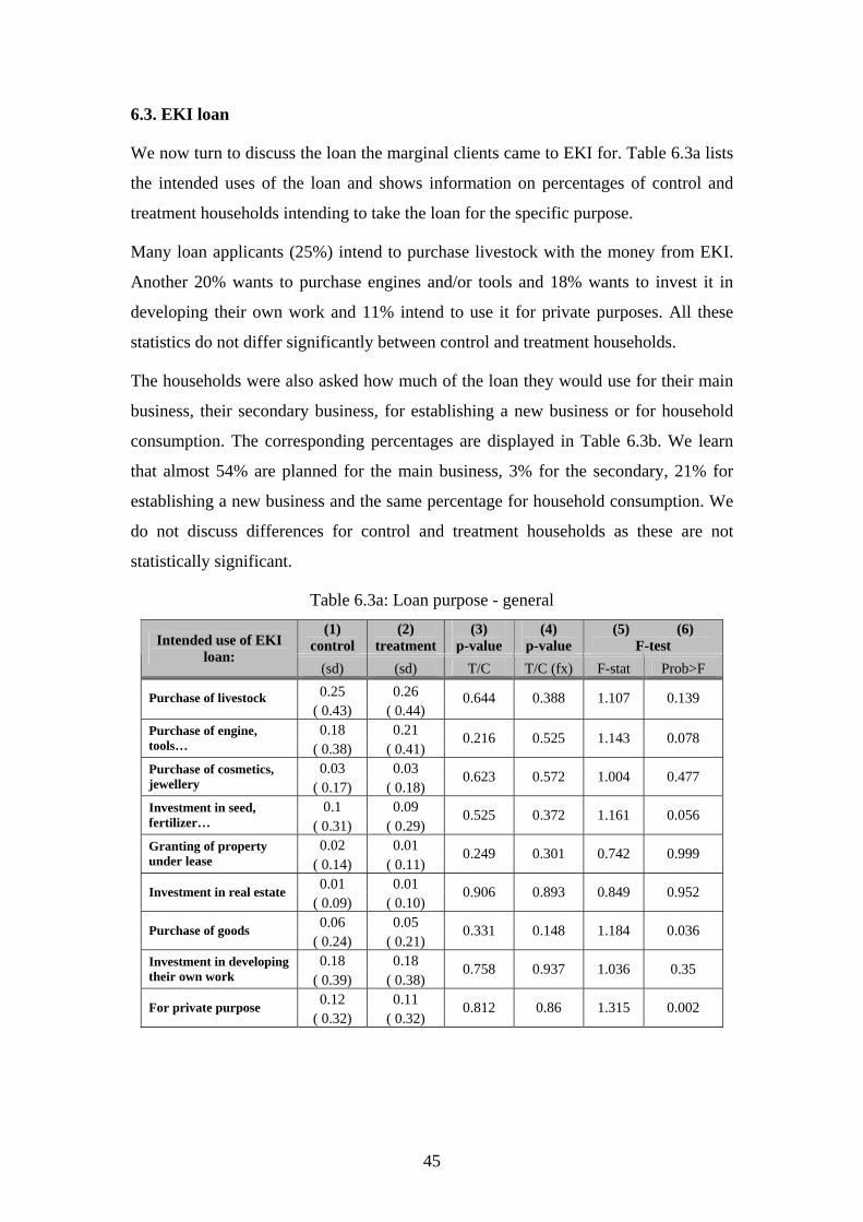
45

6.3. EKI loan

We now turn to discuss the loan the marginal clients came to EKI for. Table 6.3a lists

the intended uses of the loan and shows information on percentages of control and

treatment households intending to take the loan for the specific purpose.

Many loan applicants (25%) intend to purchase livestock with the money from EKI.

Another 20% wants to purchase engines and/or tools and 18% wants to invest it in

developing their own work and 11% intend to use it for private purposes. All these

statistics do not differ significantly between control and treatment households.

The households were also asked how much of the loan they would use for their main

business, their secondary business, for establishing a new business or for household

consumption. The corresponding percentages are displayed in Table 6.3b. We learn

that almost 54% are planned for the main business, 3% for the secondary, 21% for

establishing a new business and the same percentage for household consumption. We

do not discuss differences for control and treatment households as these are not

statistically significant.

Table 6.3a: Loan purpose - general (1)

control (2)

treatment (3)

p-value (4)

p-value (5) (6)

F-test Intended use of EKI loan:

(sd) (sd) T/C T/C (fx) F-stat Prob>F 0.25 0.26 Purchase of livestock

( 0.43) ( 0.44) 0.644 0.388 1.107 0.139

0.18 0.21 Purchase of engine, tools… ( 0.38) ( 0.41)

0.216 0.525 1.143 0.078

0.03 0.03 Purchase of cosmetics, jewellery ( 0.17) ( 0.18)

0.623 0.572 1.004 0.477

0.1 0.09 Investment in seed, fertilizer… ( 0.31) ( 0.29)

0.525 0.372 1.161 0.056

0.02 0.01 Granting of property under lease ( 0.14) ( 0.11)

0.249 0.301 0.742 0.999

0.01 0.01 Investment in real estate ( 0.09) ( 0.10)

0.906 0.893 0.849 0.952

0.06 0.05 Purchase of goods ( 0.24) ( 0.21)

0.331 0.148 1.184 0.036

0.18 0.18 Investment in developing their own work ( 0.39) ( 0.38)

0.758 0.937 1.036 0.35

0.12 0.11 For private purpose ( 0.32) ( 0.32)

0.812 0.86 1.315 0.002

46

Table 6.3b: Loan purpose - business (1)

control (2)

treatment (3)

p-value (4)

p-value (5) (6)

F-test Usage of EKI loan: Percentage (%) for…

(sd) (sd) T/C T/C (fx) F-stat Prob>F 54.42 53.41 …main business

(47.50) (47.82) 0.714 0.634 1.278 0.005

3.12 3.13 …secondary business (16.00) (15.80)

0.991 0.922 0.973 0.604

19.56 23.88 …establishing a new business (38.50) (41.32)

0.062 0.079 0.999 0.496

23.04 19.71 …household consumption (39.05) (36.80)

0.128 0.191 1.295 0.003

Households were also asked about whether they tried to get a loan from a different

source before coming to EKI. As can be seen in Table 6.3c, 10% of the sample did so.

Conditional on having contacted another source, we know that they tried on average

1.2 other sources, mainly other microfinance banks (~50%) or friends (18%).

In 75% of the cases the loan was not offered which was mainly because of other

reasons (40%) such as lack of money – see Table 6.3d. Another major reason that the

loan was not offered was lack of collateral (~33%) and in about 15% of the cases the

household does not know the reason.

Table 6.3c: Before coming to EKI - 1

control treatment control treatment Before coming to EKI (sd) (sd) # zeros # zeros 0.11 0.09 Other sources tried (%)

(1=120 obs.) (0.31) (0.29) 508 577

1.18 1.24 Number of sources tried (0.62) (0.70)

0 0

0.20 0.29 Source tried: Bank (0.40) (0.46)

49 42

0.52 0.49 Source tried: MFI (0.50) (0.50)

29 30

0.1 0.0 Source tried: Relative (0.28) (0.18)

56 57

Source tried: Friend 0.18 0.17 50 49

The 25% of households that were offered another loan before coming to EKI decided

not to take it up because of lack of endorsement (72% of ‘other reason’s is this one).

Also important was that the loan amount was considered too small (13%) or the

interest rate too high (16%).

47

Table 6.3d: Before coming to EKI - 1

control treatment control treatment Before coming to EKI (sd) (sd) # zeros # zeros 0.31 0.36 Reason loan was not offered:

not enough collateral (0.47) (0.48) 31 29

0.02 0.04 Reason loan was not offered: not enough cash flow (0.15) (0.21)

44 43

0.02 0.11 Reason loan was not offered: too much outstanding debt (0.15) (0.32)

44 40

0.20 0.13 Reason loan was not offered: unknown (0.40) (0.34)

36 39

0.44 0.36 Reason loan was not offered: other (0.50) (0.48)

25 29

0.13 0.14 Reason loan was not taken: loan amount too small (0.34) (0.36)

14 12

0.19 0.14 Reason loan was not taken: interest rate too high (0.40) (0.36)

13 12

0.00 0.07 Reason loan was not taken: other charges/fees too high (0.00) (0.27)

16 13

0.00 0.07 Reason loan was not taken: collateral asked for excessive (0.00) (0.27)

16 13

0.63 0.57 Reason loan was not taken: other (0.50) (0.51)

6 6

At the time of the interview, the respondents did not know whether they would be

selected to receive a loan or not. Therefore, it was possible to interview them about

what they intend to do in case they will not receive the loan from EKI. Slightly more

than half of the sample (51.7%) said they would try to get the money from another

source of which 43% would approach an MFI and 16% a bank.

7. Perception / Stress

In this last section on descriptive statistics of the sample, we look at the marginal

client’s view on their financial situation as well as their level of stress.

The potential marginal clients in this study decided to take on risk by making an

investment into their business and becoming indebted by doing so. We believe that by

putting them in this situation, the individuals might increase their stress level, which

in turn might influence their performance. At the same time, it is not completely

accurate to assume that it is purely external stressful situations that cause stress. If it

was the case, then everybody exposed to a particular stressor – such as the

(additional) indebtedness – would affect everybody equally. How we perceive and

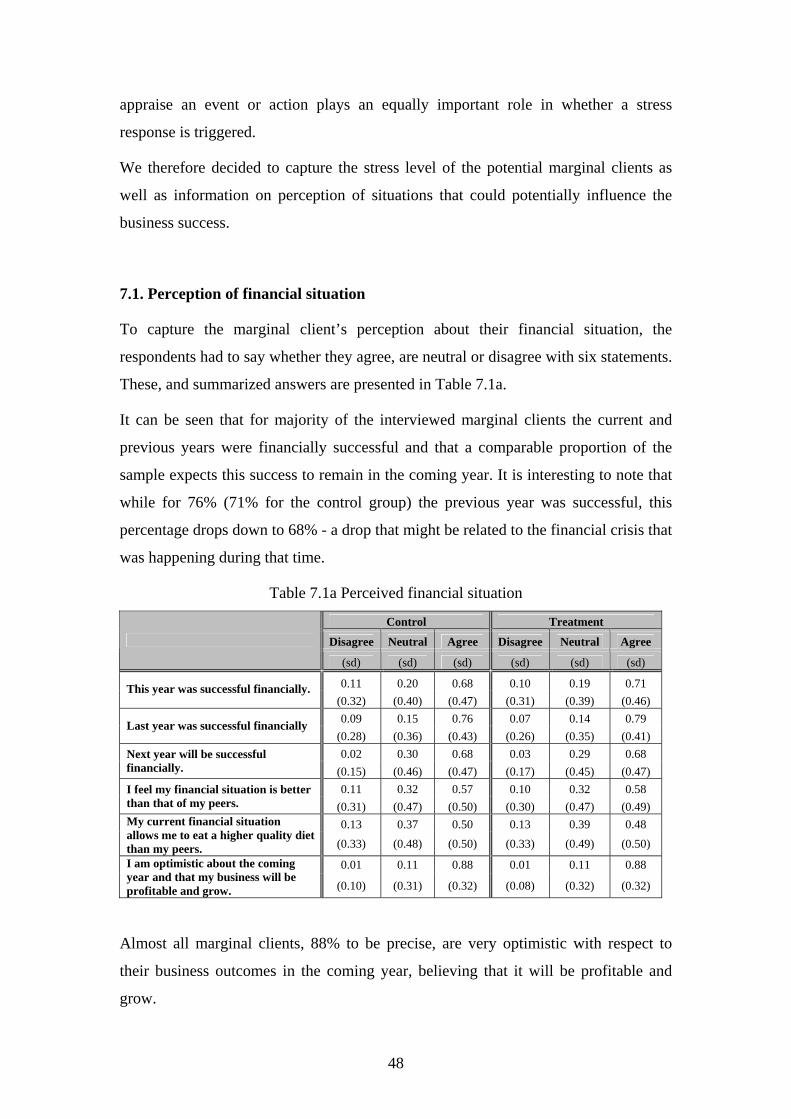
48

appraise an event or action plays an equally important role in whether a stress

response is triggered.

We therefore decided to capture the stress level of the potential marginal clients as

well as information on perception of situations that could potentially influence the

business success.

7.1. Perception of financial situation

To capture the marginal client’s perception about their financial situation, the

respondents had to say whether they agree, are neutral or disagree with six statements.

These, and summarized answers are presented in Table 7.1a.

It can be seen that for majority of the interviewed marginal clients the current and

previous years were financially successful and that a comparable proportion of the

sample expects this success to remain in the coming year. It is interesting to note that

while for 76% (71% for the control group) the previous year was successful, this

percentage drops down to 68% - a drop that might be related to the financial crisis that

was happening during that time.

Table 7.1a Perceived financial situation

Control Treatment

Disagree Neutral Agree Disagree Neutral Agree

(sd) (sd) (sd) (sd) (sd) (sd)

0.11 0.20 0.68 0.10 0.19 0.71 This year was successful financially. (0.32) (0.40) (0.47) (0.31) (0.39) (0.46) 0.09 0.15 0.76 0.07 0.14 0.79 Last year was successful financially

(0.28) (0.36) (0.43) (0.26) (0.35) (0.41) 0.02 0.30 0.68 0.03 0.29 0.68 Next year will be successful

financially. (0.15) (0.46) (0.47) (0.17) (0.45) (0.47) 0.11 0.32 0.57 0.10 0.32 0.58 I feel my financial situation is better

than that of my peers. (0.31) (0.47) (0.50) (0.30) (0.47) (0.49) 0.13 0.37 0.50 0.13 0.39 0.48 My current financial situation

allows me to eat a higher quality diet than my peers. (0.33) (0.48) (0.50) (0.33) (0.49) (0.50)

0.01 0.11 0.88 0.01 0.11 0.88 I am optimistic about the coming year and that my business will be profitable and grow. (0.10) (0.31) (0.32) (0.08) (0.32) (0.32)

Almost all marginal clients, 88% to be precise, are very optimistic with respect to

their business outcomes in the coming year, believing that it will be profitable and

grow.

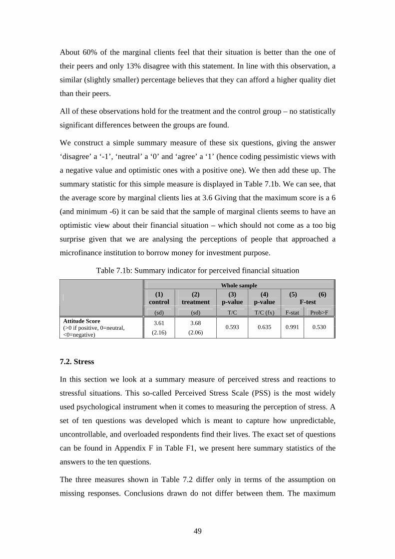
49

About 60% of the marginal clients feel that their situation is better than the one of

their peers and only 13% disagree with this statement. In line with this observation, a

similar (slightly smaller) percentage believes that they can afford a higher quality diet

than their peers.

All of these observations hold for the treatment and the control group – no statistically

significant differences between the groups are found.

We construct a simple summary measure of these six questions, giving the answer

‘disagree’ a ‘-1’, ‘neutral’ a ‘0’ and ‘agree’ a ‘1’ (hence coding pessimistic views with

a negative value and optimistic ones with a positive one). We then add these up. The

summary statistic for this simple measure is displayed in Table 7.1b. We can see, that

the average score by marginal clients lies at 3.6 Giving that the maximum score is a 6

(and minimum -6) it can be said that the sample of marginal clients seems to have an

optimistic view about their financial situation – which should not come as a too big

surprise given that we are analysing the perceptions of people that approached a

microfinance institution to borrow money for investment purpose.

Table 7.1b: Summary indicator for perceived financial situation

Whole sample (1)

control (2)

treatment (3)

p-value (4)

p-value (5) (6)

F-test

(sd) (sd) T/C T/C (fx) F-stat Prob>F

3.61 3.68 Attitude Score (>0 if positive, 0=neutral, <0=negative) (2.16) (2.06)

0.593 0.635 0.991 0.530

7.2. Stress

In this section we look at a summary measure of perceived stress and reactions to

stressful situations. This so-called Perceived Stress Scale (PSS) is the most widely

used psychological instrument when it comes to measuring the perception of stress. A

set of ten questions was developed which is meant to capture how unpredictable,

uncontrollable, and overloaded respondents find their lives. The exact set of questions

can be found in Appendix F in Table F1, we present here summary statistics of the

answers to the ten questions.

The three measures shown in Table 7.2 differ only in terms of the assumption on

missing responses. Conclusions drawn do not differ between them. The maximum

50

score a respondent can obtain is 40, the minimum is 0. A score of 40 implies that the

respondent is very stressed, according to the answers provided.

It can be seen that respondents seem to have a slightly less than average stress level

with a score of around 19 – again no significant differences for the two groups.

Table 7.2: Stress measures

Whole sample (1)

control (2)

treatment (3)

p-value (4)

p-value (5) (6)

F-test Stress Indicator (min 0, max 40)

(sd) (sd) T/C T/C (fx) F-stat Prob>F

19.21 18.97 stress indicator 1 ( 3.93) ( 4.21)

0.318 0.23 1.116 0.122

19.15 18.89 stress indicator 2 ( missing=2) ( 3.97) ( 4.30)

0.288 0.264 1.098 0.160

19.07 18.82 stress indicator 1 (missing=0) ( 4.05) ( 4.39)

0.295 0.274 1.097 0.163

8. Conclusion

The previous sections provided an in-depth look at the baseline data collected for the

Bosnian randomised field experiment on extending microfinance loans to marginal

clients. Formal tests were carried out comparing a wide range of characteristics across

the treatment and the control group. This is an important exercise because it allows us

to see how successful the randomisation procedure has been. In principle

randomisation ensures that treatment and control units are similar in expectation but

testing baseline data on ‘pre-treatment’ variables provides evidence that the

randomisation has indeed been conducted appropriately.

The results from this exercise are very encouraging: we find very few significant

differences in variables across treatment and control units, despite considering a very

large range of detailed variables. In the few cases where differences do exist, they are

generally small and do not provide any evidence of systematic differences between

treatment and control units along any particular dimension. Indeed the differences are

not jointly significant. We are therefore confident that the randomisation and

sampling of clients has been carried out appropriately and has laid down the best

possible foundation for analysing the impacts of offering loans to this poorer group of

the population.

51

9. Loan officers’ view of marginal clients

One big challenge of financial institutions is the one of information asymmetry - the

fact that loan applicants have more information about their background, motivation,

and other factors that will influence their ability to repay a loan.

A big problem that affects empirical research on these issues is the lack of reliable

data on what individuals know, or their information. It is empirically very difficult to

distinguish among different models of asymmetric information because we lack data

on what information is available to individuals and what is accessible to loan officers.

An innovative research agenda is to try to measure the relevant quantities directly.

In this study, we attempt to collect information that allows as to measure the extent of

asymmetric information between the loan officer and the potential client.

To do so, loan officers followed the normal EKI procedures as closely as possible.

This implied that they would fill-out the EKI site visit forms, collecting general

background information on the potential client, information on loan and assets; they

would do a financial analysis and write a loan review. Some of this data will be

analysed in the next section.

But, in addition to these usual procedures, loan officers were asked to fill-out a

questionnaire about the marginal client, which was developed to get an idea of the

loan officer’s perception and views with respect to the clients abilities and character.

This data will be discussed next. To start with the loan officers had to give their

judgement as to whether the marginal client conforms to the EKI requirements. The

different categories asked about were based on information from EKI on loan

appraisal procedures as well as their loan application form.

We can see in Table 9.1 that loan officers perceive 80% of marginal clients to be

credit worthy. They believe that the great majority conforms to EKI’s requirements

with respect to their credit history (86%) and their repayment capacity (76%). They

also believe that 62% of marginal clients have the appropriate business capacity. It

seems that the main reason for loan applicants to be considered as marginal clients

and so would under usual procedures not receive a loan, is insufficient collateral: only

23% of marginal clients conform to EKIs requirement within this category.

52

Table 9.1: EKI requirements

Conform to EKI requirement? (%) Obs Mean Std. Dev.

1 sufficient collateral 1072 0.234 0.424 2 repayment capacity 1069 0.756 0.430 3 credit worthiness 1068 0.804 0.397 4 business capacity 1069 0.623 0.485 5 credit history 1043 0.859 0.348 6 other 1073 0.162 0.369

Loan officers were also asked which category they find most and least worrisome –

results being presented in Table 9.2. Not surprisingly, the collateral is seen as most

worrisome. On the other hand, loan officers seem to be least concerned about credit

history (45%) as well as repayment capacity (20%) and business capacity (18%).

Table 9.2: Most/least worrisome requirement

Most worrisome Least worrisome EKI requirement

Freq. % Freq. %

Sufficient Collateral 616 63.18 68 7.22

Repayment Capacity 127 13.03 191 20.28

Creditworthiness 16 1.64 81 8.6

Business capacity 170 17.44 167 17.73

credit history 25 2.56 419 44.48

other 21 2.15 16 1.7

Next, loan officers were asked to give their impression of the applicant’s character. A

number of character traits were listed and the loan officer had to say whether s(he)

agreed or disagreed9 that the potential marginal client inhibits this character trait.

Figure 9.1 displays the distributions of the impressions of loan officers and Table 9.3

shows descriptive statistics of a summary measure, where diagreement was coded as

negative (totally disagree=-2, diagree=-1) and agreement zero or positive (somewhat

agree=0, agree=1, totally agree=2).

9 More specifically, the scale was: ‘totally agree’, ‘agree’, ‘somewhat agree’, ‘disagree’ ‘totally disagree’, ‘don’t know’.

53

Figure 9.1: Impression of applicants’ characteristics

Table 9.3: Applicants’ characteristics

Applicant appears… Obs Mean SD

…competent 965 0.883 0.698

…reliable 992 0.926 0.793

…trustworthy 978 0.746 0.657

…knowledgeable 976 0.572 0.694

…experienced 990 0.710 0.708

…well-integrated into society 956 0.508 0.754

…clever 981 0.719 0.591

…a risk-taker 960 0.436 0.715

…a fighter 966 0.859 0.726

…aggressive 934 -1.012 0.763

…stable 964 0.737 0.602

…insecure 925 -0.624 0.760

We can see that loan officers seem to have on average a quite positive impression of

the potential marginal clients. They see them as reliable, competent, trustworthy,

fighters, clever and stable. They also agree – to a somewhat lesser extend but still in

agreement - that they are knowledgeable, well-integrated into society and risk-takers.

They on the other hand do not see the applicants as aggressive or insecure.

Loan officers were then asked to judge whether they believe that these same

characteristics will influence the applicants’ business success. Table 9.4 shows their

beliefs (the coding in line with the one in Table 9.3).

54

Table 9.4: Influence on business success Characteristic […] will influence business success. Obs Mean SD

…competent 923 1.908 0.289

…reliable 923 0.922 0.390

…trustworthy 923 1.821 0.570

…knowledgeable 923 0.780 0.635

…experienced 923 1.905 0.294

…well-integrated into society 922 0.610 0.807

…clever 922 1.920 0.272

…a risk-taker 921 1.915 0.279

…a fighter 923 1.964 0.186

…aggressive 923 1.192 0.394

…stable 923 1.923 0.267

…insecure 914 -0.229 0.975

There is very strong agreement that competency, trustworthiness, experience,

cleverness, stableness and being a fighter will influence the success of the applicants’

businesses. Loan officers further agree that reliability and aggressiveness will play a

role. Less strongly, but still positive is the belief that being knowledgeable and being

well-integrated into society will help the applicants.

The final question with respect to the applicants’ character traits was which one

would be the most risky one. Table 9.5 shows that loan officers believe the risk-taking

preference of 40% of clients as a risky character trait. They also see not being well-

integrated into the society as a problem for 17% of the potential marginal clients also

not being stable and not being experienced is seen as risky in more than 10% of cases

for each character trait.

Table 9.5: Most risky character trait

Most risky character train Freq % Competent 11 1.45 Reliable 20 2.64 Trustworthy 30 3.96 Knowledgeable 44 5.80 Experienced 88 11.61 Well-integrated into society 129 17.02 Clever 3 0.40 Risk-taking 309 40.77 A fighter 20 2.64 Pushy 1 0.13 Bull-headed 18 2.37 Stable 85 11.21

55

9.1. Expectations

We described in section 6.1.1. how marginal clients were interviewed about their

expectations with respect to their business profit in the coming year.

Loan officers had to answer a similar set of questions, relating to their expectations of

the clients’ household income in the coming year.

As before, respondents were asked to state how much income they would expect the

client’s household to make over the next year if things turned out to be extremely

successful, and if things turned out to be extremely unsuccessful.

Table 9.6: Expected min and max household income

Variable Obs Mean SD Min Max Expected household income if unsuccessful 999 4,061 7,612 0 100,800

Expected household income if successful 997 8,123 14,703 250 158,400

diff (exp max - exp min) 997 4,059 8,622 80 108,000

We can see from Table 9.6 that loan officers expect the household income of marginal

clients to be about BAM 4,061 (~GBP 1,900) in the coming year if things go very

badly for the household and about BAM 8,123 (~GBP 3,800) if things go very well.

This translates into a range of BAM 4,059 between expected minimum and maximum

household income.

Comparing these numbers to household income in the previous year as reported by

the marginal client’s themselves, we find substantial differences.

Table 9.7 repeats summary statistics of information provided by the marginal clients.

In the first line we see that they had a household income of on average BAM 18,000,

which is more than twice what the loan officers expect households to earn in the

coming year if all goes extremely well. Such a big difference indicates that loan

officers might have had a different interpretation of ‘household income in mind’ than

marginal clients.

Table 9.7 also repeats summary statistics for the realized and expected business profit

as reported by the clients. We can see that, at least for the main business, also these

numbers are much higher than the expectations of the loan officers.

56

Table 9.7: Household Income and (expected) business profits as reported by the

marginal clients

Variable Obs Mean SD Min Max Total Yearly household income 1206 17,781 14,263 0 180,000

netprofit main business, last year 749 10,769 19,488 -144,000 246,000 netprofit secondary business, last year 108 5,571 6,816 -6,000 48,000 Expected profit if unsuccessful 1,105 31,700 65,878 50 840,000 Average expected profit 1,105 46,801 93,924 75 1,080,000 Expected profit if unsuccessful 1,105 61,993 125,618 100 1,320,000

Subsequently, loan officers were asked for their judgement as to the probability of the

respondent’s household receiving at least a certain amount of income in the coming

year. This threshold was calculated based on the previously given expected minimum

and maximum income.

In the piloting phase (229 interviewers), the interval between the minimum and

maximum was divided in four equally spaced intervals, so that loan officers had to

give estimated probabilities for three thresholds. This was changed to two thresholds

(hence three equally spaced intervals) after the piloting phase (761 interviews

remaining).10 The number of observations of the different versions are displayed in

Table 9.8.

Table 9.8: No of observations (different questionnaire versions)

Version Freq. Percent

1 229 21.36 2 772 72.01 3 71 6.62

Total 1,072 100

Summary statistics for the probabilities that loan officers associated with given client

specific thresholds are shown in Table 9.9. The first three rows are those for the first

(piloting) version) and the last two those for the full-survey version.

10 In 71 cases loan officers were using a wrong questionnaire file where only two thresholds were calculated but three probabilities were asked for. Despite only two thresholds being given, they still gave three probabilities and since it is not clear what numbers these are based on, we discard these observations from the analysis. In this second version, nine further observations were discarded as no probabilities were given.

57

Table 9.9: Threshold Probabilities

(1) (2) (3) Variable: probability that expected household income >= threshold A/B/C

Obs Mean SD Min Max # `0` # `50` # `100` # `wrong'

prob A 229 0.54 0.23 0.00 1.00 1 75 7

prob B 229 0.34 0.17 0.00 1.00 2 38 1 Version 1

(Piloting) prob C 227 0.24 0.16 0.00 0.95 1 20 0

26

prob A 761 0.58 0.23 0.00 1.00 8 171 13 Version 2

prob B 761 0.39 0.20 0.04 1.00 0 142 11 110

The columns labelled (1) show the standard summary statistics, with the means of the

probabilities given. We can see that, on average, probabilities decrease with

thresholds of expected household income increasing. This is in line with basic

probability laws, namely the law of monotonicity. Column (3) shows the number of

cases in which this law is violated – all together 136 cases (~14%).11

Also of interest is the extent of bunching of percentages. A clear pattern of bunching

around multiples of tens and fives can be observed (not reported in a table). This is

usually seen as a natural form of bunching as people are more inclined to round up or

down to multiples of five or ten. Of more interest is the extent of bunching of the

percent chance responses at 0%, 50%, and 100%. Results for these are reported in

columns labelled (2) in Table 9.9.

When asked for the percentage chance that next year’s overall household income will

be higher than the first (and lowest) threshold, 75 loan officers gave the mid-value of

50 per cent. Seven gave a probability of 100%, which would imply that the minimum

expected threshold was underestimated by these loan officers and one loan officer

answered 0%, which is wrong according to probability laws as it would imply that the

minimum expected income to be larger as the maximum income the loan officer

expects the client to get.

For the second threshold (the mid-point) there were 38 50s stated, two zeros and one

100. For the third threshold we find a similar pattern of 20 50s, one zero and no

100%. 11 More specifically, for the first version, probability for threshold A was smaller than probability for threshold B in four cases, Probability for threshold B was smaller than probability for threshold C in 22 cases and in one case, both of the former two cases happened.

58

Approximately the same pattern can be found for the second questionnaire version.

The final issue loan officers were asked to judge was their expectations with respect

to the applicants’ repayment history, as displayed in Table 9.10.

Table 9.10: Expectations regarding repayment

Obs Mean Std. Dev. Min Max

How likely that client will NOT be late in paying installments? 1060 0.691 0.207 0.010 1

How likely that client will be more than 1 month late in paying 1 installment?

1059 0.197 0.152 0.000 0.8

How likely that client will be late in paying more than 1 installments? 1060 0.131 0.134 0.000 0.9

On average, loan officers believe in a likelihood of 70% of marginal clients repaying

all instalments on time. They see a 20% probability of clients being more than one

month late in paying one of the instalments.

Finally, they see a probability of 13% that marginal clients will be late in their

repayment for more than one instalment.

10. Site visit forms

As part of their daily routines, EKI loan officers visit potential clients and fill out a

so-called ‘field-visit-form’ (SVF) which includes information some basic data on the

applicant, its credit history, a financial analysis on the proposed project, information

on collateral and a loan review.

We use a limited amount of this data, related to the clients’ background, to compare it

to the information we have from the household survey to get a feeling for the

accuracy of the data – assuming that the more comparable these two data sets are, the

more accurate is the information we base our analysis on.

We fist have a look at the household composition of marginal clients’ households. We

see from Table 10.1 that the mean total number of households differs slightly by 0.1

members and a similar deviation can be found when looking of the decomposition

into male and female household members. These latter two differences might result

from the fact that the information is only available for ~62% of the Site-Visit-Form

sample.

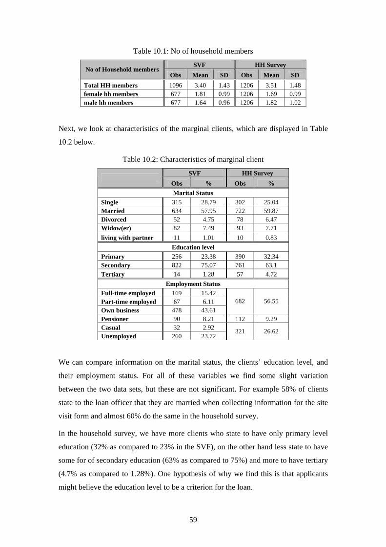
59

Table 10.1: No of household members

SVF HH Survey No of Household members

Obs Mean SD Obs Mean SD Total HH members 1096 3.40 1.43 1206 3.51 1.48 female hh members 677 1.81 0.99 1206 1.69 0.99 male hh members 677 1.64 0.96 1206 1.82 1.02

Next, we look at characteristics of the marginal clients, which are displayed in Table

10.2 below.

Table 10.2: Characteristics of marginal client

SVF HH Survey

Obs % Obs % Marital Status

Single 315 28.79 302 25.04 Married 634 57.95 722 59.87 Divorced 52 4.75 78 6.47 Widow(er) 82 7.49 93 7.71 living with partner 11 1.01 10 0.83

Education level Primary 256 23.38 390 32.34 Secondary 822 75.07 761 63.1 Tertiary 14 1.28 57 4.72

Employment Status Full-time employed 169 15.42 Part-time employed 67 6.11 Own business 478 43.61

682 56.55

Pensioner 90 8.21 112 9.29 Casual 32 2.92 Unemployed 260 23.72

321 26.62

We can compare information on the marital status, the clients’ education level, and

their employment status. For all of these variables we find some slight variation

between the two data sets, but these are not significant. For example 58% of clients

state to the loan officer that they are married when collecting information for the site

visit form and almost 60% do the same in the household survey.

In the household survey, we have more clients who state to have only primary level

education (32% as compared to 23% in the SVF), on the other hand less state to have

some for of secondary education (63% as compared to 75%) and more to have tertiary

(4.7% as compared to 1.28%). One hypothesis of why we find this is that applicants

might believe the education level to be a criterion for the loan.

60

The employment status is somewhat more difficult to compare as options do not

match exactly. The only category that should have the same definition is that of being

a pensioner (or being retired in the household survey). Here we find that 8% state to

have this employment status in the SVF and 9 in the household survey. In the

household survey we take being full-time employed, part-time employed and owning

a business together as being employed and find 56.6% to fall within this category.

This compares to 65% in the SVF data. This considerable difference may result from

the differing definitions.

Finally, we compare which business the clients’ state to be involved in, in case they

own a business. These numbers are presented in Table 10.3.

The distribution over the different categories is broadly comparable, almost the same

percentage of clients states to be involved in services (29%). The majority works in

agriculture and farming – 48% in the SVF-data and 38% in the household survey.

These differences might again be due to slightly different wording.

Table 10.3: Marginal clients’ business

SVF HH Survey Obs % Obs %

Sector of own business Sales/Trading 106 22.22 208 27.19 Maufacturing/Production 4 0.84 45 5.88 Service 140 29.34 225 29.41 Agriculture/Farming 227 47.59 287 37.52

Overall, while differences are observed between these two data sets, the results are

quite comforting. Differences that are found might be due to differing sample sizes for

certain information as well as different wording in the questions and different

categories. When the latter two coincided, statistics are much closer in values.

61

APPENDIX A1 – Presentation for Loan Officer Training (These slides were shown in Serbo-Croatian during the training sessions)

Expanding microfinance

in Bosnia & Herzegovina An EKI - EBRD impact assessment of

lending to marginal clients

Britta Augsburg (IFS) - Ralph de Haas (EBRD) - Heike Harmgart (EBRD)

Costas Meghir (IFS) - Borislav Petric (EKI)

Loan officer information sessions, Bosnia & Herzegovina, November 2008

Outline

1. Introduction: why a study on expanding outreach?

2. The marginal client3. A randomised impact assessment 4. Practical procedures of the study5. The three questionnaires6. Questions?

Introduction: expanding outreach

Microfinance in Bosnia has become very competitive

Further lending growth possible by expanding outreach to poorer clients and smaller businesses

EBRD wants to assist microfinance institutions in Bosnia such as EKI to expand outreach while remaining profitable

But what is the impact of expanding outreach on

– The profitability and sustainability of EKI?

– The economic well-being of new EKI clients?

The ‘marginal client’: a potential for new business?

Introduction: expanding outreachThe benefits for EKI

Considering marginal clients can help EKI to remain competitive and deepen its outreach to potentially good clients that are just outside the normal client base

Marginal clients are at the heart of EKIs social mission to assist in poverty alleviation and expand outreach to poorer regions

This study intends to help EKI to get a better understanding of these marginally clients

The study will result in clear recommendations about whether or not EKI should expand its lending to these marginal clients (commercial viability, poverty alleviation)

The participation in this study will contribute and prepare EKI for the possible future introduction of risk scoring

Introduction: expanding outreachThe benefits for the loan officer

Considering marginal clients can help the loan officer to expand his/her portfolio; meet monthly plans now and in the future

This study helps to expand the loan officer portfolio in a safe and controlled environment with the full support of EKI management

The study will result in clear recommendations about whether loan officers should expand the business to these marginal clients

The participation in this study will contribute and prepare loan officer for the possible future introduction of risk scoring

Introduction: expanding outreachThe potential risks for EKI

New marginal clients may have a somewhat higher chance of late repayments, a higher probability of default, and thus higher arrears

The above may result in temporary higher monitoring costs

But: - higher riskiness not for sure

- higher costs may be more than compensated by higher additional revenues

Outline

1. Introduction: why a study on expanding outreach?

2. The marginal client3. A randomised impact assessment 4. Practical procedures of the study5. The three questionnaires6. Questions?

The marginal clients

What is a marginal client?

Assume EKI would have a risk scoring system with ‘1’being the riskiest clients and ’10’ being the best clients. Anyone with score ‘6’ or higher would get a loan. We could then define the marginal clients as those with scores of ‘4’ or ‘5’

EKI: have to rely on judgement of the loan officer.

“Those clients that would only just be rejected and about whom you would keep thinking at night”

62

The marginal clients (continued)

Clients that are a little bit more risky, for instance who have collateral of bad quality

Marginal clients are not clients:– With an extremely poor credit history

– That are over-indebted

– Are suspected to be fraudulent

We expect on average ± 3-4 marginal clients per month per loan officer

Outline

1. Introduction: why a study on expanding outreach?

2. The marginal client3. A randomised impact assessment 4. Practical procedures of the study5. The three questionnaires6. Questions?

A randomised impact assessment –the methodology

Randomisation ensures that the treatment group and the control group are statistically the same in terms of both observable and unobservable characteristics

The only difference will be whether they get a loan or not

We can thus precisely and without bias measure the causal impact of the loan on various outcomes

A randomised impact assessment

Measure the causal effect of microfinance on economic wellbeing of marginal clients

– Turnover of business, income, consumption

All marginal clients will be assigned to either the treatment group (loan) or the control group (no loan)

Assignment to either group is done randomly (through a lottery with a 50% chance)

The randomisation is done on a client level but within each branch the risk of marginal clients will be spread equally amongloan officers

Outline

1. Introduction: why a study on expanding outreach?

2. The marginal client3. A randomised impact assessment 4. Practical procedures of the study5. The three questionnaires6. Questions?

Practical procedures

10-28 November: Pilot of questionnaire (BFC)

17-28 November: Pilot of the whole procedure in Gradacac and Bijeljina

8 December: study starts in 14 EKI branches

Will last for 3-4 months (until a minimum of 1,200 marginal clients have been identified and about 600 of those have received a loan)

Average loan amount maximum €1,500

Practical procedures (continued)

1. After the loan application has been entered into the PC and the sight visit the loan officer (LO) identifies a marginal client to the branch manager & credit committee.

2. The credit committee decides on the list of marginal clients

3. LO informs the client face-to-face (at the clients home) that (s)he would normally not get a loan. LO explains the study to the client. If the client wants to participate, the LO will submit the application to EBRD. It will then enter a lottery with a 50%chance of receiving a loan. The requirement is to participate ina 45 min telephone survey now and in 12 months’ time

Practical procedures (continued)

4. If the potential marginal client agrees, (s)he suggests a time within the next two days to be contacted by the survey company and participate in the telephone interview. The LO gives the participation gift and informs the client when (s)hecan expect the answer with respect to the loan application.

5. The LO sends an email to the branch manager with the name, the telephone number, the mobile number and the date and time of the telephone interview.

6. LO fills out a short questionnaire on the client and emails it to the branch manager and attaches the electronic site visit form

7. The survey company (BFC) conducts the telephone interview at the pre-agreed time and sends an email to the branchmanager (BM) when the interview is completed.

63

Practical procedures (continued)

8. The branch manager emails the details of the potential marginal clients to EBRD/IFS (including name and unique identification number), the loan officer questionnaires and the electronic sitevisit forms on a weekly basis

9. EBRD/IFS randomly select 50% of the approved marginal potential clients and will inform the branch manager about whichpotential marginal clients have been selected and may get a loan

10. These selected clients will then be automatically approved by the loan committee

11. The branch manager distributes these approved marginal clients equally among the loan officers (on a monthly average)

12. The loan officers will inform the approved clients and continue with the normal EKI lending procedure

Practical procedures (continued)

13. EKI will provide monthly excel sheet updates to EBRD on loan repayments of these clients for the period of 12 months

14. Each Branch has a target of identifying 3 marginal clients per loan officer per month

15. This process will continue until at least 1,200 potential marginal clients have been approved by the loan officers and the local loan committees and at least 600 loans have been extended

Outline

1. Introduction: why a study on expanding outreach?

2. The marginal client3. A randomised impact assessment 4. Practical procedures of the study5. The three questionnaires6. Questions?

1. The client questionnaires

Baseline survey

Follow-up survey (one year later / Spring 2010)

These questionnaires will be used to measure the impact that getting a loan may have on the marginal clients

Questions on:– Existing loans (if any)

– Household consumption, savings, income and assets

– Business activities

2. The loan officer questionnaire about the marginal clients

To be filled after the new potential marginal client has

agreed to participate

Filling out will take about 5-10 minutes

We will discuss this questionnaire in more detail after this

presentation today

Questions on:– Your assessment of the quality of the potential marginal client

– Your impression of the personality of the client

– Your expectations about the future success of the client

3. Today’s loan officer questionnaire

Questions on:– Some basic personal information

– Your work experience

– Your economic outlook

– Your processing of loan applications

– Your risk perceptions

This questionnaire is confidential, will only be used by IFS/EBRD in anonymous format, and will not be

shared with EKI management

Thank you for your attention...

... and we hope we can count

on your co-operation!

Time for questions

Heike Harmgart: harmgarh@ebrd.com

Ralph de Haas: dehaasr@ebrd.com

64

APPENDIX A2 – Loan Officer Guide for the EKI-EBRD microfinance study

Each Branch has a target of identifying 3 marginal clients per loan officer per month – so for example a branch with 20 loan officers has a monthly target of identifying 60 marginal clients; your participation for the success of the study and the expansion of EKIs business is key. By being part of this study you will contribute to expanding the outreach of EKIs microfinance to more rural and poorer clients where access to business finance will make a big difference. 1) Identifying a marginal client:

• After the loan application has been entered into the PC and the sight visit has been conducted, the loan officer (LO) identifies a client as marginal. (LO can even before filling out the electronic SVF decide whether the client is a marginal client, but in that case the electronic SVF must be filled out afterwards. In any case the file is being prepared like the file for a normal authorisation, that takes into consideration all the procedures included in the credit manual)

• The LO informs the branch manager via email about the marginal client directly after having identified a client as marginal; this email includes all the basic information that is necessary for the discussion at the credit committee;

• The branch manager creates a list of all marginal clients for the weekly credit committee meeting;

• The credit committee decides which marginal clients will be eligible for a loan (this should be done during the normal credit committee meeting after the normal loans have been decided) on a weekly basis;

• All credit committee members when discussing the marginal client should keep in mind that for these clients the credit eligibility criteria should be relaxed slightly; these discussions already include the loan features (amount (max. KM 3000); repayment period etc.);

2) Informing the marginal client: • The LO informs the marginal clients within 24 hours after the credit

committee meeting; and the LO informs the client face-to-face (at the clients home) that (s)he would normally not get a loan. LO explains the study to the client. The LO explains that if the client wants to participate, the LO will then submit the application to EBRD. It will then enter a lottery with a 50% chance of receiving a loan. Alternatively the LO can explain the selection to the client: There is a chance of receiving a loan and the final decision will be made by EBRD. The requirement is to participate in a 45 min telephone survey (conducted by BFC/PULS) now and in 12 months’ time regardless of whether (s)he will receive a loan in the coming year or not; the decision of whether the client will get a loan or not will be made independent of the answers in the questionnaire (EBRD will not have seen the answers when making the selection decision);

• It is important to explain the benefits of participating in the study well to the client in particular the chance of receiving a loan, where under normal circumstances they would not have received one (a suggested introduction can be found at the end of this document);

65

• If the potential marginal client agrees, (s)he suggests a time within the next two days to be contacted by the survey company (BFC/PULS) and participate in the telephone interview.

• The LO tells the client that they will be contacted at this pre-agreed time by the survey company (BFC/PULS);

• The LO writes down the contact details (including fixed line and mobile phone number and the ID number from the ID card) and interview time and date and the name and mobile number of two contact persons; The LO tells the client that they will be contacted at this pre-agreed time by the survey company (BFC/PULS) and should be available at this time;

• When the LO comes back from the field he fills out the questionnaire about the client (Q_LO_marg_client.xls)

• The LO fills out a form with the contact details (LO_form.xls) • The LO sends an email to the branch manager (BM) attaching the

questionnaire (Q_LO_marg_client.xls), the contact form (LO_form.xls) and the electronic site visit form (SVF);

4) Extending a loan to the marginal client: • The branch manager distributes the approved marginal clients equally

among the loan officers (on a monthly average); • The loan officers will inform the assigned and approved clients and

continue with the normal EKI lending procedure; • The loan officer informs the not selected clients that unfortunately they

have not been selected but that there opinion is very important and therefore as discussed before the survey company will call them again in 12 month time;

The study will continue until at least 1,200 potential marginal clients have been interviewed by the survey company (BFC/PULS) and at least 600 loans have been extended. Introducing the study to the marginal potential client: Mr./Ms. [Name], unfortunately your application does not qualify for a regular EKI loan. But we are currently undertaking a microfinance study together with the European Bank for Reconstruction and Development (EBRD) to see if EKI can expand its outreach to more clients like you. We have selected you to participate in this study conducted by the (EBRD). As part of this study you will have the chance of receiving an EKI loan. If you agree to participate I will submit your application to EBRD and they will make the final decision. The only requirement for a chance of receiving an EKI loan is to participate in a 45min telephone survey interview now and in one year regardless of whether your loan application has been selected by EBRD or not. Your answers in this survey don’t influence EBRD’s decision. The EBRD is helping with its investments to reduce poverty and encourage entrepreneurship in Bosnia & Herzegovina and other countries through the

66

development of their microfinance sector. EBRD has been working together with EKI since 2006 and both EKI and EBRD are committed in helping MSME clients to develop their business extend finance to grow their micro business further. With your participation in our survey you will help international organisations and EKI understand how micro-credits support clients like you in developing their business, and their personal lives during this year and how it will change by next year. Your answers to the questions on loans, the business situation and consumptions will help us develop new credit products and understand better the needs of MSME clients in BiH, and will help improve the products and services of microfinance institutions in BiH such as EKI. The information will be collected from 1200 clients then compiled in a database and analysed using statistical methods. Your name or names of your family members and data related to your business will be strictly confidential. The results will be further analysed by researchers and scientists in London. No one else will have access to your data and private information, not any banks, government officials, organizations, or persons other than those working on the survey. Your answers to the questionnaire have no influence on your chances of receiving a loan from EKI. One of the research assistants will call you for the interview within the next two days. Please let me know when it would be convenient for you [date] and [time]. Thank you for your cooperation and participation

67

APPENDIX A3 – Branch Manager Guide for the EKI-EBRD microfinance study

Each Branch has a target of identifying 3 marginal clients per loan officer per month – so for example a branch with 20 loan officers has a monthly target of identifying 60 marginal clients; your participation for the success of the study and the expansion of EKIs business is key. By being part of this study you will contribute to expanding the outreach of EKIs microfinance to more rural and poorer clients where access to business finance will make a big difference. 2) Decision on the marginal clients:

• After the loan application has been entered into the PC and the sight visit has been conducted, the loan officer (LO) identifies a client as marginal. (LO can even before filling out the electronic SVF decide whether the client is a marginal client, but in that case the electronic SVF must be filled out afterwards. In any case the file is being prepared like the file for a normal authorisation, that takes into consideration all the procedures included in the credit manual)

• The LO informs the branch manager via email about the marginal client directly after having identified a client as marginal; this email includes all the basic information that is necessary for the discussion at the credit committee;

• The branch manager creates a list of all marginal clients for the weekly credit committee meeting;

• The credit committee decides which marginal clients will be eligible for a loan (this should be done during the normal credit committee meeting after the normal loans have been decided) on a weekly basis;

• All credit committee members when discussing the marginal client should keep in mind that for these clients the credit eligibility criteria should be relaxed slightly; these discussions already include the loan features (amount (max. KM 3000); repayment period etc.);

2) Informing the marginal client: • The LO informs the marginal clients within 24 hours after the credit

committee meeting; and the LO informs the client face-to-face (at the clients home) that (s)he would normally not get a loan. LO explains the study to the client. The LO explains that if the client wants to participate, the LO will then submit the application to EBRD. It will then enter a lottery with a 50% chance of receiving a loan. Alternatively the LO can explain the selection to the client: There is a chance of receiving a loan and the final decision will be made by EBRD. The requirement is to participate in a 45 min telephone survey (conducted by BFC/PULS) now and in 12 months’ time regardless of whether (s)he will receive a loan in the coming year or not; the decision of whether the client will get a loan or not will be made independent of the answers in the questionnaire (EBRD will not have seen the answers when making the selection decision);

• It is important to explain the benefits of participating in the study well to the client in particular the chance of receiving a loan, where under normal circumstances they would not have received one (a suggested introduction can be found at the end of this document);

68

• If the potential marginal client agrees, (s)he suggests a time within the next two days to be contacted by the survey company (BFC/PULS) and participate in the telephone interview.

• The LO tells the client that they will be contacted at this pre-agreed time by the survey company (BFC/PULS);

• The LO writes down the contact details (including fixed line and mobile phone number and the ID number from the ID card) and interview time and date and the name and mobile number of two contact persons; The LO tells the client that they will be contacted at this pre-agreed time by the survey company (BFC/PULS) and should be available at this time;

• When the LO comes back from the field he fills out the questionnaire about the client (Q_LO_marg_client.xls)

• The LO fills out a form with the contact details (LO_form.xls) • The LO sends an email to the branch manager (BM) attaching the

questionnaire (Q_LO_marg_client.xls), the contact form (LO_form.xls) and the electronic site visit form (SVF);

3) Communication of the client details between EKI and BFC/PULS:

• Use of Google Spreadsheets • A major innovation which resulted from this project was the use of

Google Spreadsheets to share information. Problems were anticipated with the data exchange protocol because excel versioning and importing of records from the 3 parties who would be involved. It was possible for records to be lost in the shuffle and much time to be spent copying data and verifying it.

• BFC proposed the use of Google Docs to create an online spreadsheet which can be accessed by branch managers, PULS, BFC and EBRD. Google Spreadsheets work like a basic version of Excel but is web based. Up to 50 individuals can work on the file at once, revision histories are kept and it can be exported to Excel for more advanced analysis. Also, BFC exported the files on a regular basis to ensure a backup/archive copy. This option was proposed to EBRD and EKI and was accepted by all

• The branch managers (BM) of the 14 EKI branches enter http://docs.google.com and open the ebrd_eki_puls_pilot_v2 spreadsheet. The BM completes columns D-N on the sheet for his/her branch. The Usernames and Passwords are provided directly to the Branch Manager.

• The interview times will be within the next 48hours of being entered; 4) Conducting the interview:

• PULS opens the spreadsheet and looks for new interviews scheduled daily.

• PULS enters interview information into CATI system and completes columns B and C.

• PULS calls the clients at the pre-agreed time and conducts the interview. Scheduling is managed by the CATI system.

• PULS updates columns O-S by Thursday at 15:00 CET. 5) Selection of the clients that will receive a loan:

69

a. On Friday EBRD/IFS will select randomly 50% of the completed interview clients and communicate them to EKI branch managers to be automatically approved and receive a loan;

b. IFS will enter a “Y” into the pink column T for the selected clients that will receive an EKI loan and “N” for those not selected.

c. EKI will inform both the EBRD selected that their application has been approved and the non-selected that their application has not been selected by EBRD;

d. EKI then continues with their normal lending procedure for those clients and not lend to the ones not selected for 12 month

5) Informing EBRD on the repayment of these new clients: • The branch manager will provide monthly excel sheet updates to EBRD

(EBRD will create a separate account for this project and all its email correspondence) on loan repayments of these clients (EBRD will send a proposal for this excel sheet to EKI) for the period of 12 months.

The study will continue until at least 1,200 potential marginal clients have been interviewed by the survey company (BFC/PULS) and at least 600 loans have been extended.

70

APPENDIX B - Expected outcomes sample design and precision

We consider a number of outcomes including outcomes for the firm and the household. In order to design the experiment and decide on the sample size we need to have some idea of the magnitude of the effects we can reasonably expect. Putting it differently, what kind of effects could we expect for such an intervention, were the intervention to be useful and successful? Of course it is all down to the investment returns. On the one hand the clients are capital poor, which on the basis of standard economic theory of decreasing returns should make the returns particularly high. Judging by the huge interest rates that moneylenders charge in developing countries, some individuals may reasonably expect returns of 100% or more. On the other hand poor individuals with low levels of education and skills may have difficulty converting the loan to a highly profitable return. We use three approaches to gauge the minimum return that we could expect to detect and which would make the intervention successful.

a) The first approach defines what we can reasonably expect to see from a successful and needed programme if the average loan to the new group equals the average microfinance loan currently observed – this assumes a rate of return of investment of 10% over and above the costs of servicing the loan b) The second approach considers the maximum amount of the loan that the average household could take up given observed earnings and consumption (in 2004), c) the final approach is the more traditional evaluation approach that considers the potential costs of the loan and defines the minimum acceptable effect we would wish to see to justify continuing the intervention. It turns out that all approaches imply that a successful programme would lead to about 3% increase in consumption. However, the final “cost of programme” approach could also imply a required effect for a successful programme as low as 0.6%.

In the first approach we assume that our new target population will receive loans of equivalent magnitude to the loans already in place. The average microfinance loan in

Bosnia is Euro 800. The interest rate on the microfinance loan is about 20%. So for the loan to improve standards of living of the household the return should be higher than that (in nominal terms). In the presence of tight liquidity constraints, which after all is the motivation of such programmes it is not unreasonable to expect such high returns. A reasonable return for the household, over and above the cost of the loan could be taken to be 10% of the original loan value, i.e. Euro 80. According to the LSMS annual consumption in 2004 for an average household was Euro 3100. Under this scenario we can expect a successful policy to increase consumption by 2.6% under the assumption that the households believe they will always have access to this finance. Any overall growth effects due to the permanent alleviation of liquidity constraints will not be visible because they are likely to also affect the control group in the experimental evaluation.

The second way to look at the problem is to calculate the amount of a loan that they could possibly finance. In this case we assume that the loan will be for one year (at least in the first instance). Based on LSMS 2004 the average household has total earnings of Euro 4500. The average expenditure is Euro 3100; this leaves 1400 potential savings.

71

Assuming this is the maximum that they could then borrow (including interest), would imply a loan of Euro 1200 with a return for the household of Euro 120 annually, consumption should increase by 3.9%.

An alternative third way of looking at the issue is in terms of the ability of the programme to cover its costs: we could define the desired effect as the effect that we would need to justify the costs of the programme. What are the costs of the programme? Based on past experience, with a less risky population most of the loans will be repaid on time, with arrears currently at less than 2%. Suppose as an extreme that arrears represent a full loss of the principal and interest we can say that the average cost of a loan is 2.4% of the value advanced. Hence any effect that would increase consumption on average by more than 2.4% of the value of the loan would constitute a positive effect of the programme. For the average loan, which is 800 Euro we would thus require an increase in consumption of at least 19 Euros, which is a very small effect indeed. On the basis of the current experience, the lowest increase in consumption which could justify the programme, if the default rate for the new population is the same as the current one being serviced is 0.6%. If we now suppose that the complete default rate in the riskier group is 10%, the loss including interest will be 12% of all loans advanced, implying an required increase in average consumption of at least 100 Euros or for the average loan and family consumption observed an increase in consumption by more than 3.2%. Given the return to investment assumed above (10% above the costs of servicing the loan) a default rate higher than this would probably mean the programme would not be successful. Thus calibrating the sample size to be able to detect a 3% increase in consumption may be a sensible approach.

From the above it seems that we would need sample sizes that would allow us to detect an effect of consumption of between 2.5% and 4%. In practice this will very much depend on the size of the loans advanced. It is quite clear that detecting effects of loans smaller than Euro 800 may be difficult, unless we expect gross returns much higher than 30%.

In the Tables below we present different levels of predicted standard errors for the programme effect, depending on the achieved follow-up sample size by outcome variable and by whether we obtain baseline data so as to measure growth. It is important that we do not rely on recall data for these variables.

We now turn to the predicted precision for key household level outcomes based on the World Bank LSMS data.

Because we are designing an evaluation based on a randomised experiment the effects can be computed simply as the difference in the mean between the treatment and the control group. Under the null hypothesis of no programme effect the variance of the outcome of interest will be the same in the treatment and control groups. Denote this variance by 2σ . Assume that the size of the treatment group (those chosen to receive loans) is equal to the size of the control group (those not chosen) and denote this by N.

Thus the full sample size is 2N. Moreover by allocating half the overall sample to treatment and half to control we achieve an optimal sample design.

Denote the estimated effect (impact) by β̂ . Then the variance of β̂ is Var( β̂ ) = 2 2σ /N.

72

Thus the desired sample of treatments (and equal number of controls) to achieve a

standard error of )ˆ(βVar is N = 2 2σ / Var( β̂ ). To obtain suitable sample sizes we need to obtain estimates of σ2, which we do using the LSMS data from the World Bank. Based on this data we present the standard errors we would obtain for different values of N after conditioning on characteristics that cannot be affected by treatment and that we can hope to observe when we collect our data. These characteristics include age, marital status, household size and composition. The relevant outcome variance then is the residual variance.

The LSMS is a panel and we can thus condition on predetermined variables to further reduce the outcome variance 2σ . These lagged values can mimic the information we obtain at baseline. However, the predetermined variables we will condition on to estimate precision are lagged three years; hence the reduction in the outcome variance is probably lower than what would have been achieved if we could condition on variables one year before.

In Table A.1 below we present anticipated standard errors for a number of outcome variables at different sizes of the treatment group. We present a version based on using only contemporaneous characteristics (no baseline data) and using lagged values of the outcomes (with baseline data)

The achievable standard errors presented in Table 1 relate to monthly earnings including the zeros for those who do not work measured in BiH currency, to log consumption and to employment. The average monthly earnings level is the LSMS is 276 for men and 107 for women when zero earnings are included for those not working.

To interpret the numbers for log consumption note that the effects are log points or approximately percentage increases when multiplied by 100. So a standard error of 0.1 implies a confidence interval for the estimated effects of approximately ±0.2 or ±20% points on the outcome.

With a sample of 500 treatments we will be able to detect changes in earnings in excess of BiH 550 annually for men and 360 for women as well as well as about 6% increases in household consumption and 6% increases in employment for women and 4% for men. It is unlikely that the one of loan of about 800 Euros will be able to achieve such large effects. Thus unless the intervention offers much larger loans we will need to contemplate sample sizes of over 1000 in the treatment group and equivalently in the controls. The Table also shows that with 1500 observations in the treatment group we can be confident of detecting the kind of effects we can reasonably expect the programme to have on individual standard of living.

One notable characteristic of these results is that we do not achieve a huge improvement in the standard errors by using lagged values of outcome variables, despite the fact that these are significant determinants. However, we could hope for a

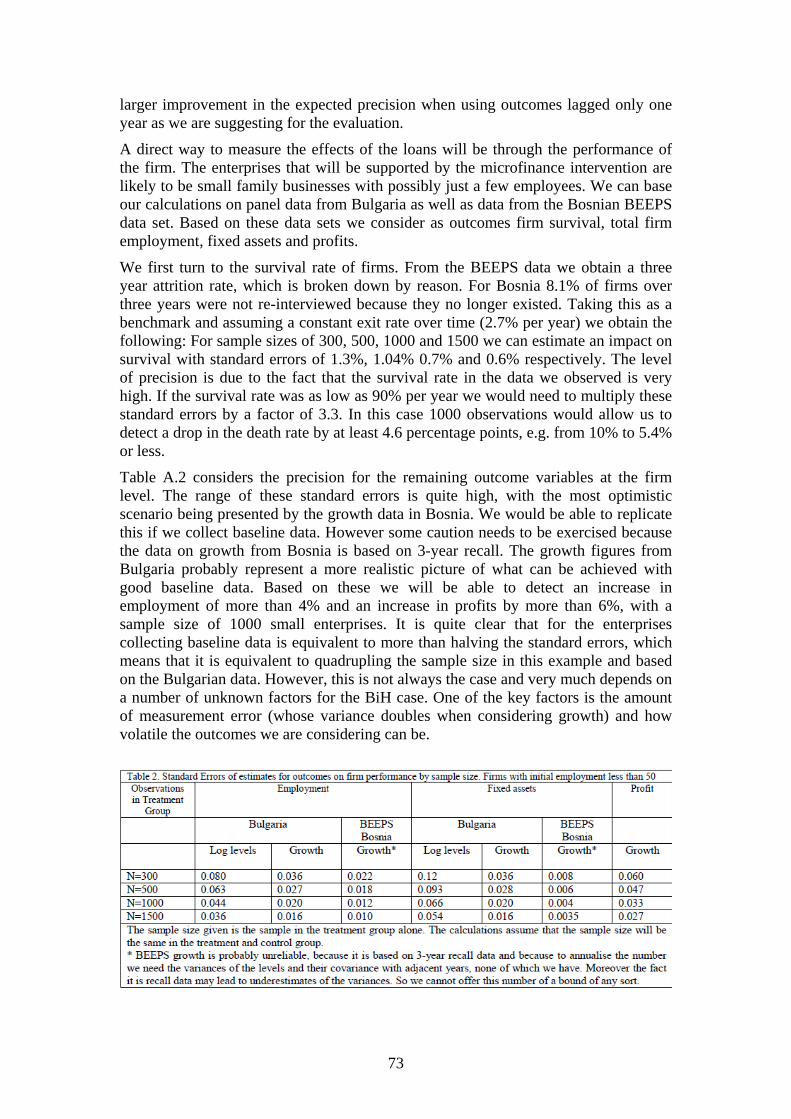
73

larger improvement in the expected precision when using outcomes lagged only one year as we are suggesting for the evaluation.

A direct way to measure the effects of the loans will be through the performance of the firm. The enterprises that will be supported by the microfinance intervention are likely to be small family businesses with possibly just a few employees. We can base our calculations on panel data from Bulgaria as well as data from the Bosnian BEEPS data set. Based on these data sets we consider as outcomes firm survival, total firm employment, fixed assets and profits.

We first turn to the survival rate of firms. From the BEEPS data we obtain a three year attrition rate, which is broken down by reason. For Bosnia 8.1% of firms over three years were not re-interviewed because they no longer existed. Taking this as a benchmark and assuming a constant exit rate over time (2.7% per year) we obtain the following: For sample sizes of 300, 500, 1000 and 1500 we can estimate an impact on survival with standard errors of 1.3%, 1.04% 0.7% and 0.6% respectively. The level of precision is due to the fact that the survival rate in the data we observed is very high. If the survival rate was as low as 90% per year we would need to multiply these standard errors by a factor of 3.3. In this case 1000 observations would allow us to detect a drop in the death rate by at least 4.6 percentage points, e.g. from 10% to 5.4% or less.

Table A.2 considers the precision for the remaining outcome variables at the firm level. The range of these standard errors is quite high, with the most optimistic scenario being presented by the growth data in Bosnia. We would be able to replicate this if we collect baseline data. However some caution needs to be exercised because the data on growth from Bosnia is based on 3-year recall. The growth figures from Bulgaria probably represent a more realistic picture of what can be achieved with good baseline data. Based on these we will be able to detect an increase in employment of more than 4% and an increase in profits by more than 6%, with a sample size of 1000 small enterprises. It is quite clear that for the enterprises collecting baseline data is equivalent to more than halving the standard errors, which means that it is equivalent to quadrupling the sample size in this example and based on the Bulgarian data. However, this is not always the case and very much depends on a number of unknown factors for the BiH case. One of the key factors is the amount of measurement error (whose variance doubles when considering growth) and how volatile the outcomes we are considering can be.

74

The estimates of the anticipated standard errors of the effects obtained from the Bosnian BEEPS data should be treated with extreme caution for the following reasons:

a) They are based on three year recall data b) To obtain the annual variance, used in the calculation of the standard error, we

have treated successive realisations of growth as independent and identically distributed random variables, an assumption that is almost certainly untrue. This assumption probably leads to an upward bias

However, because we do not know how recall biases the variance of the growth rate we cannot assume that the estimate the predicted standard errors given in the table and based on the BEEPS data, is an upper bound.

75

APPENDIX C – Characteristics female marginal clients

Table C1: Characteristics of female marginal clients

control treatment Female Respondents

(sd) (sd) Age 37.84 38.69 (11.69) (11.99) Marital status 0.62 0.6 (1=married) ( 0.49) ( 0.49) Economic status 0.42* 0.45* (1=employed) ( 0.49) ( 0.50) Economic Status 0.29 0.28 (1=unemployed) ( 0.46) ( 0.45) Some primary 0.35 0.4* school ( 0.48) ( 0.49) Some secondary 0.59* 0.53* school ( 0.49) ( 0.50) Some university 0.05 0.07* education ( 0.23) ( 0.26) No of hours worked 36.98* 38.69* (per week) (27.93) (26.90) No of hrs worked in 28.61* 31.69 Business (p week) (25.42) (25.50) Stars indicate a significant difference between male and female respondents

76

APPENDIX D – Socio-Economic Household Indicators

Table D1: Household asset value, by item

Whole sample Conditional on owning the asset (1)

control (2)

treatment (3)

p-val (4)

p-val (5) (6)

F-test control treatment contr. treat. Value of…

(sd) (sd) T/C T/C (fx) F-stat Prob>F (sd) (sd) # zeros # zeros

80967 76693 88106 83411 …house(s) (87152) (68065)

0.354 0.297 1.264 0.007 (87386) (66919)

48 44

33234 39474 48026 59055 ...land (ha parcels) (76799) (130110)

0.354 0.376 0.892 0.869 (88423) (155527)

187 150

3060 3404 5669 6311 ...cars (5283) (7055)

0.342 0.39 1.013 0.438 (6078) (8601)

292 261

1386 2095 10240 14831 ...lorry, tractor, boat… (4746) (20215)

0.414 0.318 0.703 1.000 (8744) (52242)

547 492

1737 1711 4016 3777 ...animals (cattle, pigs, horses…) (4107) (4800)

0.922 0.608 1.517 0.000 (5469) (6568)

343 319

108 133 257 322 ...motorbike/bike(s) (312) (458)

0.282 0.304 1.05 0.300 (440) (669)

373 329

297 291 837 825 ...computer/notebook/ printer (605) (564)

0.867 0.944 1.034 0.357 (764) (681)

409 366

2210 2004 3500 3238 ...tools for business and private purpose and other machinery (6891) (10110)

0.685 0.831 1.633 0.000 (8411) (12701)

239 206

502 485 2595 2616 ...inventory/stock/ unsold merchandise (2329) (3620)

0.924 0.792 0.557 1.000 (4769) (8094)

518 458

240 245 252 256 ...mobile phone(s) (261) (264)

0.746 0.848 1.276 0.005 (262) (264)

29 28

374 382 379 390 ...tv, satellite dish (363) (407)

0.71 0.735 0.963 0.645 (362) (407)

12 8

102 96 135 131 ...video, dvd, radio, cd (129) (122)

0.413 0.516 0.966 0.633 (133) (125)

172 140

98 88 148 128 ...other small electric appliances (211) (136)

0.334 0.355 1.013 0.438 (244) (147)

196 193

19 15 913 713 ...electro-generator (183) (143)

0.619 0.442 0.889 0.882 (914) (735)

622 556

402 410 412 416 ...refrigerator, cooler (308) (324)

0.696 0.867 0.869 0.921 (305) (322)

10 13

226 205 258 252 ...electric/gas stove/oven (189) (183)

0.048 0.032 1.143 0.078 (181) (171)

118 70

295 298 335 350 ...washing machine (195) (277)

0.841 0.854 1.53 0.000 (173) (268)

94 67

2178 3079 12773 17992 ...other things (10547) (18243)

0.301 0.333 0.792 0.991 (22836) (41098)

528 472

77

Table D2: Household income sources, % (1)

control (2)

treatment(3)

p-value (4)

p-value (5) (6)

F-test Income Source (sd) (sd) T/C T/C (fx) F-stat Prob>F 0.78 0.78 Self-employment

(0.41) (0.41) 0.979 0.98 1.04 0.335

0.11 0.11 Wages from Agric. Work (0.31) (0.31)

0.833 0.553 1.157 0.060

0.08 0.07 Wages from manufacturing industry (0.26) (0.25)

0.669 0.859 0.959 0.660

0.49 0.49 Wages from other private business (0.50) (0.50)

0.95 0.569 1.097 0.162

0.13 0.12 Wages from government (0.34) (0.33)

0.575 0.512 1.128 0.099

0.21 0.21 Migration income / remittances (0.41) (0.41)

0.987 0.496 1.096 0.163

0.29 0.32 Benefits from government (0.45) (0.47)

0.244 0.166 1.295 0.003

0.34 0.32 Pensions (0.47) (0.47)

0.464 0.891 0.983 0.563

0.03 0.04 Income from rental properties (0.18) (0.20)

0.413 0.439 0.984 0.560

Table D3: Household savings, reason

Reason 1 Reason 2 Reason 3 control treatment controltreatment controltreatment Reason for savings (%)

(cond. on having savings) (sd) (sd) (sd) (sd) (sd) (sd) 0.23 0.27 0.03 0.03 0.02 0.03 for future business

expenses (0.42) (0.44) (0.18) (0.16) (0.14) (0.16) 0.09 0.11 0.08 0.09 0.01 0.01 education

(0.29) (0.31) (0.27) (0.29) (0.10) (0.09) 0.08 0.06 0.1 0.1 0.06 0.03 medical expenses

(0.28) (0.24) (0.31) (0.30) (0.24) (0.16) 0.08 0.09 0.03 0.02 0.01 0.02 provide for old age

(0.28) (0.29) (0.17) (0.14) (0.10) (0.14) 0.03 0.03 0 0.01 0.02 0.02 house repair

(0.17) (0.18) (0.00) (0.11) (0.14) (0.13) 0.37 0.35 0.17 0.17 0.06 0.08 emergency events

(0.48) (0.48) (0.38) (0.37) (0.24) (0.27) 0.04 0.03 0.02 0.02 0.01 0.03 to secure consumption

(0.21) (0.17) (0.14) (0.14) (0.10) (0.16) 0 0 0 0 0 0 pay for debt

(0.00) (0.00) (0.00) (0.00) (0.00) (0.00) 0 0 0 0 0.02 0 festival expenses

(0.00) (0.07) (0.07) (0.00) (0.16) (0.00) 0.01 0.02 0 0.02 0 0 other

(0.12) (0.13) (0.00) (0.13) (0.00) (0.00)

78

APPENDIX E – Third loan of marginal clients

Table E1: Characteristics of the 3rd Loan:

Loan 3 control treatment control treatment

Loan Characteristics

(sd) (sd) # zeros # zeros

0.48 0.39 Provider: Bank (0.51) (0.50)

11 14

0.52 0.52 Provider: MFI (0.51) '(0.51)

10 11

0.00 0.09 Provider: Other (0.00) (0.29)

21 21

3738 3975 Loan Amount (3133) (3647)

0 0

155.00 273.89 Monthly Payment (74.94) (545.66)

0 0

2.00 1.90 Interest rate known (%) (0.00) (0.30)

0 0

. 33.00 Interest rate (1.41)

0 0

29 28 repayment period (months) (17.84) (24.79)

0 0

2343 2523 Amount outstanding (2379 (4970)

0 0

49.52 36.67 % used for business (49.24) (48.30)

10 13

Table E2: Characteristics of the 3rd Loan - continued

Loan 3 Collateral 1 Collateral 2

control treatment control treatment Collatoral Provided

(sd) (sd) (sd) (sd) 0 0 0 0 House 0 0 0 0 Machinery

0.01 0.01 0 0 Own salary '(0.10) '(0.08) '(0.06)

0 0 0 0 spouse salary

0.03 0.05 0.01 0 family member/ relatives salary / co-signer '(0.18) '(0.21) '(0.10)

0 0 0.00 0 Other

0.02 0.00 0 0 Don't know '(0.12) '(0.05)

79

APPENDIX F – Stress questions

Table F1: Stress Questions

STRESS

0 = Never 1 = Almost Never 2 = Sometimes 3 = Fairly Often 4 = Very often

10.1. In the last month, how often have you been upset because of something that happened unexpectedly? 0 1 2 3 4

10.2. In the last month, how often have you felt that you were unable to control the important things in your life?

0 1 2 3 4

10.3. In the last month, how often have you felt nervous and "stressed"? 0 1 2 3 4

10.4. In the last month, how often have you felt confident about your ability to handle your personal problems?

0 1 2 3 4

10.5. In the last month, how often have you felt that things were going your way? 0 1 2 3 4

10.6. In the last month, how often have you found that you could not cope with all the things that you had to do?

0 1 2 3 4

10.7. In the last month, how often have you been able to control irritations in your life? 0 1 2 3 4

10.8. In the last month, how often have you felt that you were on top of things? 0 1 2 3 4

10.9. In the last month, how often have you been angered because of things that were outside of your control? 0 1 2 3 4

10.10. In the last month, how often have you felt difficulties were piling up so high that you could not overcome them?

0 1 2 3 4

80

REFERENCES Armendariz de Aghion, B and J. Murdoch (2005), The Economics of Microfinance,

Cambridge, MA: MIT Press.

Banerjee, A., E. Duflo, R. Glennerster and C. Kinnan (2009), The miracle of microfinance? Evidence from a randomized evaluation, available at www.povertyactionlab.com.

Augsburg, B. (2009), The impact of a dairy intervention in rural India: evidence from realised outcomes and expected returns to investment, Journal of Development Effectiveness, 1(2), 147–170.

Hartarska, V. and D. Nadolnyak (2007), An impact analysis of microfinance in Bosnia and Herzogovina, William Davidson Institute Working Paper No. 915.

HBS (2007), The household budget survey 2007 – poverty and living conditions, Published by the Bosnia and Herzegovina Agency for Statistics of Bosnia and Herzegovina.

Karlan, D. and J. Zinman (2009), Expanding microenterprise credit access: Using randomized supply decisions to estimate the impacts in Manila, available at www.povertyactionlab.com.

National Human Development Report (2009). The ties that bind – social capital in Bosnia and Herzegovina, United Nations Development Programme (UNDP) in Bosnia and Herzegovina, Sarajevo.