1

Microfinance and Moneylenders: Long-run Effects of MFIs on Informal Credit Market in Bangladesh

Claudia Berg1 George Washington University

M. Shahe Emran IPD, Columbia University

Forhad Shilpi World Bank

September 5, 2013

ABSTRACT Using two surveys from Bangladesh, this paper provides evidence on the effects of microfinance competition on village moneylender interest rates and households’ dependence on informal credit. The views among practitioners diverge sharply: proponents claim that MFI competition reduces both the moneylender interest rate and households’ reliance on informal credit, while the critics argue the opposite. Taking advantage of recent econometric approaches that address selection on unobservables without imposing the standard exclusion restrictions, we find that the MFI competition does not reduce moneylender interest rates, thus partially repudiating the proponents. The effects are heterogeneous; there is no perceptible effect at low levels of MFI coverage, but when MFI coverage is high enough, the moneylender interest rate increases significantly. In contrast, households’ dependence on informal credit tends to go down after becoming MFI member, which contradicts part of the critic’s argument. The evidence is consistent with a model where MFIs draw away better borrowers from the moneylender, and fixed costs are important in informal lending. Key Words: Microfinance, Moneylenders, Microcredit, Interest Rates, Informal Borrowing, Long-run Effects, Bangladesh, Identification through Heteroskedasticity JEL Codes: O17, O12, C31

1 We would like to thank Dilip Mookherjee, Will Martin,Wahiduddin Mahmud, Pallab Mozumder, and participants

in Canadian Economic Association annual conference 2013, IGC South Asia conference in Dhaka in July 2012, and Development workshop at GWU for helpful comments. We owe a special debt to Frank Vella for extensive discussions and guidance on heteroskedasticity based identification. For access to data, we are grateful to Mahabub Hossain (household Panel data) and Wahiduddin Mahmud and Baqui Khalily (village cross-section data). We benefited from discussions with Zabid Iqbal on the InM-PKSF cross-section survey. Emails for correspondence: cberg@gwmail.gwu.edu, shahe.emran@gmail.com, fshilpi@worldbank.org. The standard disclaimers apply.

2

1. INTRODUCTION

Concerns about exploitative moneylenders and usurious interest rates have motivated a variety of

government interventions in rural credit markets for centuries in many countries: anti-usury laws, debt

settlement boards, credit cooperatives (IRDP in India, ‘Comilla Model’ in Bangladesh), specialized rural

banks are among the well-known examples. 2 From its inception in the early 1970s in Bangladesh, a

central goal of the current microfinance movement has also been to free the poor from the “clutches” of

moneylenders, as Muhammad Yunus, the founder of Grameen Bank, puts it.3 Unlike the standard banks

that rely on collateral for screening and enforcement, the MFIs focus on rural poor without collateral,

previously served only by informal financiers: friends, family, and especially village moneylenders. The

number of poor served by microfinance institutions (MFIs) globally has increased exponentially from

10,000 in 1980 to more than 150 million in 2012. The goal of this paper is to analyze the effects of MFI

expansion on the informal credit market with a focus on the moneylenders.

The available evidence shows that government interventions in the rural credit market in the

1960s and 1970s largely failed to drive out the moneylenders (For discussion on the performance of

government policy interventions, see McKinnon (1973), Von-Pischke et al. (1983), Hoff et al. (1993),

Armendariz and Morduch (2010), Morduch and Karlan (2010)). Has the microfinance movement fared

any better in delivering the rural poor from the “clutches” of moneylenders? The proponents of

microfinance note that while the government credit programs were captured by the large landholders

(Von-Pischke et al. (1983)), MFIs target land-poor households, usually bypassed by the formal banks,

who also constitute the bulk of the clientele for the moneylenders. Unlike the government banks, the

MFIs thus can create effective competition for the moneylenders. The availability of microcredit at

relatively lower interest rates without any collateral allows poor households to substitute away from the

high interest rate loans from traditional moneylenders and landlords. Microcredit thus is expected to drive

down the moneylender interest rate and eventually drive them out of business as the microcredit market

deepens.

Many critics and observers of MFI movement, however, contend that microfinance in fact leads

to a higher demand for moneylender loans which drives up the interest rates. A household might find it

2 References to moneylenders appear throughout history, for example in the Hindu religious Vedic texts in ancient India dating back to 1500 BC. The Bible tells a story in which Jesus “overthrew the tables of the moneychangers” (Matthew 21:12-13). Perhaps the most colorful reference to a moneylender is that of Shakespeare’s Shylock who demanded his pound of flesh in exchange for a late repayment (Merchant of Venice). 3 Recounting the origin of Grameen Bank, Yunus states: “(W)hen my list was done it had the names of 42 victims. The total amount they had borrowed was US $27. What a lesson this was to an economics professor who was teaching about billion dollar economic plans. I could not think of anything better than offering this US $27 from my own pocket to get the victims out of the clutches of the moneylenders.” Yunus (2009, 7th Nelson Mandela Lecture. Emphasis added).

3

necessary to borrow from moneylenders or other informal sources after becoming a MFI member, for

example, to keep up with a rigid repayment schedule even though it did not borrow from them before (see

Sinha and Matin (1998) for discussions in the context of Bangladesh). The demand for informal loans

(and informal loans in general) may also increase because of indivisibility of investment projects; MFI

borrowers may require additional loans to achieve economies of scale in their microcredit financed

investment.4 It is often argued that the ability to borrow from multiple sources may lead to unsustainable

debt accumulation and condemn the poor to a vicious cycle of poverty and indebtedness.

While many practitioners would probably concur with one or the other contrasting views noted

above, the interactions between the informal credit market and MFIs may be much more complex and

nuanced. For example, there can be a “cream skimming” effect where the MFI poaches away the better

borrowers from the moneylender, and facing a worsened borrower pool (due to adverse selection and

moral hazard) the moneylender needs to charge a higher interest rate (Bose (1998)). Another channel that

gives rise to a positive effect of MFI penetration on moneylender interest rates, along with a reduction in

rural poor’s dependence on moneylenders, is noted by Hoff and Stiglitz (1998): if there are significant

fixed costs in screening and enforcement, competition from MFIs may force a moneylender to increase

the interest rate to cover fixed costs as the number of borrowers decline.

Since moneylenders have always been at the core of policy discussions on rural financial sector

reform, one would expect the interactions between MFIs and moneylenders to be a fruitful ground for

empirical research. It is thus surprising that there is little systematic evidence on the effects of MFIs on

the informal credit market in general and on the moneylenders in particular. The only paper of which we

are aware is Mallick (2012) that uses data for 106 villages from Bangladesh, and reports evidence of a

positive effect of MFI competition on moneylender interest rates, but the effects on households’ demand

for informal loans are not analyzed. A positive effect on moneylender interest rates in itself, however,

does not tell us that it is an outcome of higher demand; it may also result from a change in the

composition and size of the pool of borrowers in the informal markets, as noted above. To sort out the

underlying mechanism(s), we need to understand the effects of MFI membership on the household

borrowing. An analysis of both household-level loan demand and village level interest rate allows us to

differentiate between alternative hypotheses. For example, if we find that MFI penetration leads to higher

incidence of household borrowing from moneylenders along with higher interest rates, this is more

consistent with the demand shift explanation discussed above. In contrast, if we find that MFI

membership reduces the probability of a household borrowing from the moneylender, but the

4 This seems plausible given the recent evidence that the entrepreneurial MFI borrowers cut their consumption to undertake indivisible investments (see Banerjee et al. (2013)).

4

moneylender interest rates increase with MFI competition, the evidence would be more consistent with

the view that emphasizes the cream skimming effect of MFIs and fixed costs in informal lending.

Using two surveys from Bangladesh, this paper provides evidence on the effects of MFI

penetration in the rural credit markets on moneylenders’ interest rates and households’ demand for

informal loans. Bangladesh offers an excellent opportunity to understand the long run effects of MFI

penetration on informal credit markets, because it is among the most mature MFI markets in the world

with almost 40 years of microcredit lending. In 2011, there were 35 million MFI borrowers in

Bangladesh with 248 billion taka in outstanding loans (Microfinance Regulatory Authority, Bangladesh

Bank, 2009). According to estimates from various available data sources, approximately 40 percent of

the households in rural areas are now MFI members (for example, HIES, 2010). We use two rich data

sets for the empirical analysis: (i) an exceptionally large cross section data set that includes almost 800

villages in North-Western Bangladesh for the years 2006-2007, collected by the Institute of Microfinance

(InM) in Dhaka, and (ii) a panel dataset that covers from 2000 to 2007, collected by BIDS-BRAC.5 The

large cross-section data-set with almost 800 villages provides adequate power to estimate the effects on

village level moneylender interest rate with a measure of confidence, because there is ample variation in

the degree of MFI penetration across different villages.

For identification of the effects of higher MFI coverage on the moneylender interest rate in a

village, the main challenge is unobserved village-level heterogeneity. When we run an OLS regression of

moneylender interest rates on MFI coverage, the estimated effect is likely to be biased, because the MFIs

do not choose the location and intensity of credit programs across villages randomly.6 The MFIs may

target relatively well-off (productive) villages to ensure high enough repayment rates to attract or retain

donor funding. If repayment is the overriding objective, the OLS estimate might find a spurious positive

effect of MFI coverage on moneylender interest rate, driven by a higher aggregate demand for credit due

to the higher productive potential of the village. On the other hand, their location choices might be

primarily driven by poverty alleviation objectives and we would observe them to expand programs in

relatively poor, less productive, and risk-prone villages. Under this alternative case, one might find a zero

or even negative effect of MFI coverage on the interest rate in an OLS regression, even if the true causal

effect is positive. For the identification of the effects of MFI membership on the demand for

moneylender loans (or loans from informal sources, in general) by the households, we also have to worry

about self-selection by the households. The MFI participants may be systematically different from the 5 The InM survey was led by Baqui Khalily and Abdul Latif, and the BIDS-BRAC surveys by Mahabub Hossain and

his collaborators. 6 Note that the spatial heterogeneity observed in the MFI activities across villages in Bangladesh is an outcome of

MFI choices, donor policy, historical accidents, and path dependence over a period of almost 40 years. This also implies that it may not be feasible to study the long-run effects of MFI competition by randomized interventions across villages.

5

nonparticipants in the same village in terms of unobserved characteristics such as entrepreneurial ability

and risk aversion. The unobserved village and household level heterogeneity can bias the estimated

effects of MFI competition on moneylender interest rate, and on household’s demand for informal loans,

and it is not in general possible to pin down the directions of such bias from theoretical reasoning alone.

A standard approach to tackling the omitted variables bias is to design an instrumental variables

strategy. However, it is extremely difficult, if not impossible, to find credible exclusion restrictions

required for the instrumental variables approach in our application, and there has been increasing

skepticism about the validity of the exclusion restrictions imposed in many related contexts. We thus take

advantage of advances in econometrics that provide alternative ways to address omitted variables bias

without imposing exclusion restrictions; in particular, we implement minimum-biased (MB) propensity

score reweighting estimator proposed by Millimet and Tchernis (forthcoming), and heteroskedasticity

based identification scheme developed by Klein and Vella (2009a). While the propensity score

reweighting estimators (e.g., IPW) rely on the conditional independence assumption (CIA), the MB

estimator is attractive because it minimizes the bias arising from possible violation of the CIA due to

selection on unobservables. Building on an insight originally due to Wright (1928), heteroskedasticity

based identification approach was developed in a series of papers by Rigobon (2003), Klein and Vella

(2009a, 2010) and Lewbel (2012). The intuition behind heteroskedasticity-based identification is that

when there is substantial heteroskedasticity in the treatment equation, the changing variance in the

residual acts as “probabilistic shifter” of the treatment status, similar to the shifts induced by a standard

instrumental variable satisfying exclusion restriction (for an excellent discussion, see Rigobon (2003)).7

The observed heteroskedasticity in the treatment equation in our application has clear theoretical

foundations; the heteroskedasticity results from interactions between fixed costs in establishing a new

branch and private information of loan officers on potential borrowers. For the household level analysis,

we exploit a two-round panel data set spanning seven years, and combine a difference-in-difference

model with household fixed effects (DID-FE), and then implement different estimators including

matching and MB estimator in the DID-FE model.8

Our main findings are as follows. The evidence strongly suggests that penetration of microfinance

in a village increases the moneylender interest rate when the MFI coverage is high enough. At low levels

of MFI coverage, there is no perceptible effect the moneylender interest rate. The ‘proponent’s view’ that

competition from MFIs brings down the ‘exploitative’ interest rates thus seems to be contradicted.

7 For recent applications of heteroskedasticity based identification, see Rigobon (2003), Rigobon and Rodrik

(2005), Maurer et al. (2012), Klein and Vella (2009b), Farre et al. (2012, 2013), Schroeder (2010), Gilchrist and Zakrajsek (2012), Emran and Hou (2013), and Emran and Shilpi (2012), Emran et al. (forthcoming), among others. 8 For discussions on the advantages of combining matching with a DID design, see Heckman et al. (1998) and

Blundell and Costa-Dias (2009).

6

However, the results do not support the alternative view that when a household becomes an MFI member

it is more likely to take additional loans from moneylenders and other informal sources. Evidence on a

household’s propensity to borrow from informal sources based on panel data analysis shows that the MFI

membership reduces significantly the probability that a household would borrow from them. Thus the

moneylender interest rate may go up in a village even though MFI borrowers substitute away from

moneylenders as argued by the proponents of microfinance. The coexistence of higher interest rate with a

lower propensity to borrow is consistent with higher transactions costs in serving a smaller number of

clients (fixed costs) by the moneylender and higher risk premium due to cream skimming by MFIs.

The remainder of the paper is organized as follows: Section 2 is devoted to the analysis of the

effects of MFI competition on moneylender interest rate at the village level; Section 3 deals with the

effects of MFI membership on household borrowing. In each section, we first discuss the empirical issues

and our identification approach, then data, and finally present the results. The paper concludes with a

brief summary of the results.

2. THE SPREAD OF MICROFINANCE AND MONEYLENDER INTEREST RATE

2.1. EMPIRICAL STRATEGY

To understand the identification issues, consider the following triangular model:

(1)

(2)

Where, is the moneylender interest rate, is an indicator of MFI coverage in village j,

and is a set of village controls as well as regional fixed effects. We use binary indicators of MFI

activities in a village at different thresholds of coverage. This is motivated by two considerations. First, a

binary treatment allows us to take advantage of recently developed econometric approaches for non-

experimental data in the evaluation literature (for example, the Minimum Biased (MB) propensity score

reweighting estimator). Second, and no less important, it provides a simple way to analyze potentially

heterogeneous effects of MFI penetration. The effects of MFI coverage on informal interest rates are

unlikely to be constant across the distribution; its strength will, in general, depend on the extent of

coverage with possible threshold effects. One would not expect much of an impact of MFI entry into a

village on the informal interest rate if, for instance, only a small fraction of potential informal borrowers

get access to microcredit.9 A focal threshold for defining the binary ‘treatment’ is the mean coverage

9 One might wonder whether a continuous treatment variable in a quadratic specification could better capture the

heterogenous effects. The evidence presented later shows that the effects on interest rate are insignificant for the first

7

rate (42 percent in our sample of villages). We also use other thresholds for defining the treatment

variable. Note that one has to be careful about the appropriate treatment and comparison groups and the

interpretation of the estimates when the binary treatment is defined in terms of other thresholds. For

example, consider the case when the treatment is defined as villages that have MFI coverage in the top

quartile of the sample. To keep the comparison group same as the case of binary treatment defined at the

cut-off of mean coverage rate, we need to exclude the villages that fall in the third quartile of coverage

distribution.

The main identification challenge in estimating the effect of MFI penetration on moneylender

interest rate is that, in general, the correlation between and is non-zero due to unobserved village

characteristics such as productivity and risk. For concreteness, consider the implications of unobserved

productivity heterogeneity. The rural credit markets are in general segmented because of inadequate

infrastructure and the local information advantages enjoyed by moneylenders (Hoff and Stiglitz (1993),

Ghosh, Mookherjee and Ray (1999), Banerjee (2003), Siamwalla et al. (1993), Aleem (1993)). In a

segmented market, interest rates charged by the moneylenders in a village depend on its productivity

characteristics; the moneylenders in a more productive village are able to charge higher interest rates as

they extract the surplus from borrowers. If the MFIs also prefer to locate in villages with higher

productive potential, then we would observe Cov ( , . This implies that if one runs OLS

regressions, the estimated effect of MFI presence on moneylender interest rate across villages will be

biased upward; one may find a spurious positive “effect”, even if the causal impact of MFIs on

moneylender’s interest rate is in fact negative. However, the omitted productivity heterogeneity in OLS

regressions may as well lead to a downward bias in the estimated effect of MFI penetration; this happens

when the location choices of MFIs are primarily driven by poverty alleviation objectives. In this case, the

MFIs target relatively less productive villages and we expect Cov ( , . This implies that the OLS

estimate may spuriously find a zero or even a negative effect, when the true effect is positive and large in

magnitude. Possible measurement errors in the MFI coverage variable would also bias the estimated

effect towards zero due to attenuation.

A standard solution to the omitted variables bias is to employ an instrumental variables strategy.

To develop an instrumental variables strategy for credible identification, we need an exogenous source of

variation in the placement of MFI branches which does not affect the interest rate across villages. The

available studies on the location choices of MFIs in Bangladesh suggest that MFIs take into account both

profit and poverty alleviation in their location choices (Salim (2011)). The evidence also indicates that three quartiles of MFI coverage, and becomes both statistically and numerically significant only at the fourth quartile. Fitting a quadratic model in this case could lead us to erroneously conclude that there is a positive effect for the third quartile, for example. Moreover, a quadratic model involves two endogeneous variables, complicating the identification and estimation substantially.

8

the MFIs prefer villages closer to the market centers (usually the Thana center where the branch office is

located) (see, Mallick and Nabin (2010), and Zeller et al. (2001)). However, any area characteristics that

may have determined the placement of MFI branches (e.g. population density, infrastructure, poverty

indicators) can potentially affect moneylender interest rate as well. Thus they are not likely to satisfy the

exclusion restrictions required for identification.

(2.2) IDENTIFICATION WITHOUT STANDARD EXCLUSION RESTRICTIONS

Matching, Propensity Score Reweighting, and Minimum Biased Estimator

To reduce potential bias in the OLS estimates, we use three alternative estimators: matching,

“normalized inverse probability weighted (IPW)” estimator developed by Hirano and Imbens (2001) and

‘minimum biased (MB)’ estimator due to Millimet and Tchernis (forthcoming).10 The IPW estimator

weighs the observations on the treatment group by the probability of being treated (the inverse of the

propensity score) and weighs the observations on the control group by the probability of not being treated

(one minus the inverse of propensity score). Busso et al. (2011) provide extensive Monte Carlo evidence

that the normalized IPW estimator performs best among a wide set of matching and propensity score

based estimators in applied settings. The MB estimator relies on the normalized IPW, but uses an

appropriately trimmed sample to minimize the bias arising from a failure of the conditional independence

assumption. For the empirical implementation, we employ a relatively wider radius of the neighborhood

around the bias minimizing propensity score, equal to 0.25 which means that at least 25 percent of the

both the treatment and control groups have a propensity score in this interval used in the estimation. The

MB estimates reported later in this paper also correct for deviations from normality assumption using

Edgeworth Expansion. The Monte Carlo evidence shows that the MB estimator with reasonably wide

radius provides reliable estimates of causal effects for the relevant treatment group even when the

conditional independence assumption is violated because of omitted variables (Millimet and Tchernis

(forthcoming)).

Heteroskedasticity Based Identification: Klein and Vella (2009a) Approach

We noted earlier that it may not be impossible to find plausibly exogenous characteristics of a

village that are important determinants of location and intensity of MFI programs, but such village

characteristics are unlikely to satisfy exclusion restrictions imposed in the interest rate equation. As

discussed by Klein and Vella (2009a) and Lewbel (2012), existence of significant heteroskedasticity in 10Although the recent revival of IPW owes a lot to Hirano and Imbens paper, the idea can be traced back at least to Horvitz and Thompson (1952).

9

the treatment equation provides a plausible source of identification in such cases. A substantial

econometric literature has developed that exploits heteroskedasticity for identification when no credible

instrument is available (Wright (1928), Rigobon (2003), Klein and Vella (2009a, 2010), Lewbel (2012)).

The intuition behind this identification approach is that heteroskedasticity works as an exogenous

‘probabilistic shifter’ of the endogenous treatment variable (which, in our application, is the dummy for

high MFI coverage in a village). Analogous to the standard instrumental variables, this probabilistic

shifter helps us to trace out the causal relationship between the dependent variable (informal interest rate)

and endogenous treatment variable (dummy for high MFI coverage).

We utilize an approach developed by Klein and Vella (2009a) to estimate the effects of MFI

penetration on moneylender interest rate. Evidence from a number of recent Monte Carlo exercises shows

that the Klein and Vella (2009a) approach is effective in correcting for biases from omitted variables and

measurement errors (Ebbes et al. (2009), Millimet and Tchernis (forthcoming), Millimet (2011), Klein

and Vella (2009a, 2010)). The main sources of heteroskedasticity in the treatment equation need to be

identified from a priori theoretical reasoning based on intimate knowledge of the selection process.

For identification, an essential requirement in Klein and Vella (2009a) approach is that the error

term in equation (2) exhibits substantial heteroskedasticity. Let (

) be the conditional variance

function for satisfying the following condition:

( )

, (3)

Where is a zero mean homoskedastic error, is a subset of

consisting of variables that

generate heteroskedasticity and ( ) is a non-constant function. The relationship in equation (3) has

clear economic interpretation. Suppose is a measure of the intrinsic productivity attributes of area j

observed and used by MFIs for the branch location decisions, but unobserved by the econometrician.

What condition (3) above implies is that although MFIs (the central office) base their decisions on

indicators of intrinsic productivity of area j, the actual outcome (e.g. coverage rate) is determined by

interactions between productivity and other physical and socio-economic conditions (e.g. infrastructure,

land distribution, poverty incidence) as determined by the function. In the context of our application,

the function captures primarily the effects of screening by loan officers based on their private

information (for more on this, see below).

What are plausible sources of heteroskedasticity in equation (2) above? The variables potentially

giving rise to heteroskedasticity can be identified from a theoretical model that focuses on the interaction

among fixed costs in program placement (such as establishing a branch office), MFI screening and

households’ self-selection. The basic argument is simple and grounded on the available evidence; given

10

fixed costs, once a branch is placed in a village by the central office,11 the branch manager tries to achieve

a minimum scale for the viability of the program.12 In fact, ‘building volume’ and retaining borrowers are

among the most important challenges faced by MFIs when opening branches in new locations.13 The set

of potential clients is determined by the intersection of self-selection by households and MFI program

selection criteria (set at the central office). When the potential client base is not large, to achieve scale

economies, the loan officers have incentives to ignore private information on households’ credit

worthiness or eligibility. Because the private information of loan officers on households is probably the

most important component of the error term , ignoring this private information reduces the variance in

observed coverage.14 In other words, the coverage rate would tend to bunch at around the minimum

viable scale, similar to a corner solution.15 In contrast, when a large proportion of households satisfy the

program-specified criteria, the loan officers do not worry about minimum viable scale, and their private

information plays an important role in determining the actual coverage rate, resulting in a higher variance.

Variance in the coverage rate across villages in this case would reflect closely the variance in the village

and household characteristics relevant for repayment capacity and poverty alleviation and observed by the

program manager and loan officers, but not observed by the econometrician.

In the context of Bangladesh, there are plausible reasons to expect that indicators of poverty

incidence and of landlessness in a village would generate heteroskedasticity in the treatment equation.

The recent evidence on “revealed objective functions” of MFIs based on the branch locations of Grameen

Bank and BRAC in Bangladesh suggests that the MFIs take into account both poverty alleviation and

financial sustainability in their branch location decisions (Salim (2011)). The MFIs thus primarily target

the moderate poor, and exclude the extreme poor or so-called ultrapoor (Rabbani et al. (2006), Rahman

(2003)). The extreme poor may also self-select out of such programs, because they lack the required

human capital, and the substantial time commitment required for group meetings etc. may be too onerous

when they are working long hours on low-return activities for survival (Matin et al. (2008), Rabbani et al.

(2006), Emran et al. (forthcoming)). Thus the set of potential clients available to a loan officer is expected

to be higher in areas with high incidence of moderate poverty, but lower where extreme poverty is

11

The central offices (“head office”) of most of the MFIs in Bangladesh are located in the capital city, Dhaka. 12 Recent evidence shows that there are significant scale economies in microfinance (Hartarska et al. (2013)). 13In the context of Bangladesh, Rahman (2003) notes “(A)chievement of financial sustainability of a branch of MFI requires an increase in the number of clients within the branch”. To achieve scale economies, many MFIs provide incentives to loan officers to increase number of borrowers through bonuses linked to number of new clients. 14

In some cases, the loan officers may even bend the formal program criteria to attain the minimum viable scale. This may explain part of the “targeting errors” observed in MFI programs. Also, note that the self-selection by the household is necessary but not sufficient for MFI membership, because the loan officers are the “final arbiter” in selection into a program. 15

Although the MFIs in Bangladesh are known to cross-subsidize programs, closure of branches is not unheard of. Even the most successful NGOs such as BRAC have closed failing branches in the recent past.

11

prevalent. Many MFIs including Grameen Bank and BRAC use land ownership as a salient targeting

mechanism, a household with more than half acre (50 decimal) of land is in principle not eligible for the

microcredit programs. However, extreme poverty is closely linked to landlessness, and one widely used

indicator of extreme poverty is whether a household owns less than 10 decimal of land (for example, it is

used by ultra-poor programs such as BRAC CFPR/TUP). Thus households with lower than 10 decimal

land may be more likely to be excluded from and/or opt-out from the microcredit programs. Many MFIs

also use possession of a VGD card as an indicator of moderate poverty; for example, a household with

VGD card is not eligible for the ultrapoor program of BRAC.16 Thus one would expect that the client

base for standard microfinance is higher in a poor village (with higher proportion of VGD card), but

lower where proportion of landless (less than 10 decimal land) households is higher. As discussed above

in section (2.2), this implies that the error term in the MFI coverage equation will have lower variance

where the proportion of landless households is higher, and higher variance where the proportion of the

moderately poor (with VGD card) is higher (the actual coverage is to the right of the minimum viable

scale, determined by loan officers’ private information). It is important to appreciate that the a priori

signs of the heteroskedasticity-generating variables in the selection and heteroskedastic probit models

together provide economic rationale to our identification approach.

The probability of ‘high’ MFI coverage in village j can be written as:

( )

( )

(4)

Where P (.) is the distribution function of . With homoskedastic errors, ( ) is a constant;

the only source of identification is possible non-linearity of the P (.) function such as a Normal CDF in a

Probit model. Such identification relies on a small fraction of observations at the tails of the distribution,

and hence is considered unreliable (Altonji et al. (2005), Klein and Vella (2009a)). In the presence of

heteroskedasticity, ( ) is no longer a constant, and identification exploits observations from regions

where P (.) is approximately linear. In this case, the predicted probability from the estimation of equation

(2) becomes a valid instrument for identifying the effects of MFI penetration on moneylender interest

rate. Note also that if heteroskedasticity in the residual of equation (2) is weak, ( ) has little

variations (approximately a constant), and the predicted probability is a weak instrument that relies only

on the functional form of the CDF for identification. 17 In terms of the model of MFI location and

16

One might wonder if some other measures of moderate poverty based on standard poverty line estimates would be more suitable for our analysis. However, note that we are trying to capture the information set available to and used by the loan officers. While VGD card status is used by NGOs for screening, we are not aware of loan officers in any NGO in Bangladesh using village specific poverty line estimates for screening and selection. 17 A limitation of heteroskedasticity-based identification is that it is applicable only when the outcome variable is continuous. Moreover, since the estimator relies on second moments, the estimates are likely to be less efficient

12

program intensity discussed above, this can happen when the program coverage in most of the villages is

close to the minimum viable scale.

(2.3) DATA

The village level data for the econometric estimation of the impact of MFI coverage on informal

interest rate come from the baseline survey conducted during 2006-2007 by Institute of Microfinance

(InM) for the Programmed Initiative for Monga Eradication (PRIME) of Palli Karma Sahayak Fundation

(PKSF). We call the dataset the InM-PKSF survey. The baseline survey consists of a census of all

households meeting certain income, employment and land ownership criteria as well as a village level

survey.18 The village level survey collected information on moneylender interest rates and availability of

infrastructure and services. Empirical analysis of this paper is based on this village level dataset

supplemented with MFI coverage rates calculated from the household survey.19 The dataset covers three

districts (Lalmonirhat, Nilphamary and Gaibandha) in Rangpur division where the earliest baseline

surveys of the PRIME program were conducted. Out of 18 upazilas (sub-districts) in these districts,

survey was undertaken in 12 upazilas. There are 804 villages in our dataset. To make sure that our

estimates are not unduly influenced by a few outliers, we exclude a small number of villages reporting

unusually high interest rate (above 180 percent) from our sample giving us a final sample of 793

villages.20 We, however, emphasize that none of the qualitative conclusions from the empirical analysis

are affected if we use the full sample (results are available from the authors).

The InM-PKSF survey is particularly suitable for our empirical analysis for a number of reasons.

First, the survey was primarily targeted to poor households which are usually more dependent on the

moneylenders in the absence of MFIs. Second, interest rate data were collected for a standardized loan

product. The interest rate analyzed in this paper is the money lender interest in normal times (not the lean

season) for loans of duration up to one year.21 We do not include interest rates on longer maturity loans,

because the maturity of the standard MFI loans in Bangladesh is one year. The standardized rates ensure

that variations in interest rates across villages are not due to heterogeneity in loan duration or seasonality.

The summary statistics in appendix Table A.1 show considerable variations in both MFI coverage and

informal interest rates. The average informal interest rate in our sample villages is about 19 percent. This than the standard IV estimates (Lewbel (2012)). The inefficiency of the estimator implies that if we find a statistically significant effect, it should be interpreted as strong evidence. 18 Households meeting any of the following three conditions were included in the survey: households should have monthly income of Tk. 1,500 or below, or are dependent on day-labor, or have less than 50 decimal of land. 19 The household level dataset available to us does not contain the interest rate information on informal loans. 20

There is however no village which reported an informal interest rate between above 120 percent and below 180 percent. 21

The questionnaire clearly asked about moneylender interest rate (“Mohajoni Rin” in Bengali). So it is highly unlikely, if not impossible, that the households confused moneylender loans with loans from friends and family.

13

might seem low when compared to some of the estimates reported for informal interest rates in South

Asian countries for earlier periods.22 However, it is comparable to the recent estimate for West Bengal

reported by Maitra et al. (2013) (25 percent average). It is important to appreciate that the extremely high

moneylender interest rates reported in the press and many earlier studies refer primarily to short-term

consumption loans taken to tide over a few weeks or months during the lean season.23 We also divide

villages into quartiles in terms of MFI coverage rate. The average interest rates are comparable across the

three lower quartiles, but rise to 27 percent for the topmost quartile. Note that the moneylenders charge

interest on loans at a flat rate, and thus the effective interest rate is much higher when the declining

balance over time is taken into account; a 27 percent flat rate is approximately equal to a 60 percent

effective rate, assuming that the repayment schedule is similar to a standard MFI loan product.24 As is

widely discussed in the microcredit literature, MFIs also calculate flat rate interest and thus the rates are

comparable to the moneylender interest rates. The average interest rate charged by MFIs in Bangladesh

has been around 15 percent (flat rate) in recent years, according to CGAP. Estimates based on data from

Credit and Development Forum for the year 2000 show that 80 percent of MFIs in Bangladesh charge 11-

15 percent interest rate, and about 1 percent charges more than 20 percent (Rahman (2003)). Starting

from July 2004, the wholesale microcredit fund provider PKSF capped the interest rate at 12.5 percent

flat.

The average MFI coverage rate is about 42 percent in our sample of villages (Table A.1) which is

comparable to coverage rate from our panel data (38 percent). According to the Household Income and

Expenditure Survey (HIES) 2010, about 45 percent of households with less than an acre of land in the

Rangpur division covering areas included in our sample are active borrowers from MFIs. The summary

statistics for all other variables used in the regression are also reported in Table A.1.

(2.4) OLS, MATCHING AND IPW ESTIMATES

We start with the simplest specification where the moneylender interest rate is regressed on the

MFI coverage dummy (D=1 if coverage in a village more than the mean coverage rate) without any

controls. The OLS estimate, reported in column (1) of Table 1, shows a statistically significant and

positive correlation. This positive ‘effect’, however, could result from common unobserved village 22 According to one estimate reported in late eighties, the average interest rate charged by moneylenders was 51.86 percent in rural India (Dasgupta, 1989); Aleem (1993) reports an average lending rate of 78.5 percent in Pakistan. For a summary of the evidence on informal interest rates in developing countries see Banerjee (2003). 23

It is not uncommon to have 25-50 percent interest rate for a consumption loan for a month, which becomes extremely high interest rates when annualized. Most of the moneylender interest rates reported in the literature are annualized rates on short term consumption loans. 24

Note, however, that it assumes that the repayment schedule is enforced strictly, which is unrealistic, for both the moneylender loans and MFI loans.

14

characteristics. If better infrastructure and higher productivity of a village lead to both higher informal

interest rate and better coverage of MFIs, then one would expect this correlation to weaken when we add

controls for village productivity and infrastructure.

In the next specification, we add several controls for village productivity and risk characteristics

which can also potentially affect MFI placement. Access to markets and other services is measured by

average distances to bazar (market), bus stop and secondary school. Distance to formal bank branch is

introduced to capture potential competition from and linkages to the formal financial sector (Bell (1993)).

Irrigation increases productivity and reduces risk of agricultural production, affecting both risk and

returns in the credit market. Accordingly, we include percentage of households using irrigation as a

control. We also include the number of households surveyed in a village as a scale variable. Vulnerable

Group Development (VGD) is a major public safety net program targeting the poor in Bangladesh; many

NGOs also use the VGD cards as an indicator of moderate poverty. For example, the BRAC excludes a

household from its ultra-poor program (CFPR/TUP) if it has a VGD card. We use percentage of

households with VGD cards as an indicator of moderate poverty in the village.25 Land ownership is used

by most of the MFIs as a salient selection criterion. While many MFIs including BRAC, Grameen Bank,

and BRDB in principle lend only to households owning less than 50 decimal of land, mis-targeting due to

both type 1 and type 2 errors is not uncommon. In particular, the evidence indicates that landless (owning

less than 10 decimal of land) are largely excluded from the standard MFI lending programs. Thus the

landless constitutes an important clientele of moneylenders. We include the percentage of landless (less

than 10 decimal) in the village to capture this effect. When these controls are added to the specification,

the results (column 2) indicate a much larger effect of MFI coverage in the interest rate regression. In

columns (3) and (4), we add district and upazilla fixed effects as catch-all controls for time-invariant

unobserved village heterogeneity respectively. The coefficient of MFI coverage becomes slightly larger

in column (4) compared with column (1). Both estimates (columns (3) and (4)) are statistically significant

at the 1 percent level. What is striking though is the fact that instead of weakening, the partial correlation

between informal interest rate and MFI coverage has become numerically and statistically more

significant when village productivity controls are added. This suggests that, in our application, MFI

location choices are driven largely by poverty alleviation objectives, and thus OLS coefficients are likely

to be biased downward.

The OLS regressions in Table 1 (columns (2) and (3)) identify a number of salient correlates of

moneylender interest rates. Interest rates are lower in villages with higher irrigation coverage. More

irrigation means lower risk and higher productivity (through green revolution varieties). Though higher

25

We emphasize again here that we are using VGD card instead of a village level “poverty line” to define the extent of moderate poverty, because the MFI loan officers do not rely on village level poverty line estimates (if available).

15

productivity may allow moneylenders in a segmented market to charge higher interest rates, the OLS

results suggest that the lower risk premium predominates over the productivity effect. Interest rates are

higher in more isolated villages (far from market centers). As the market segmentation is likely to be

more severe in remote villages, moneylenders can, ceteris paribus, extract more rent by charging higher

interest rates. Interest rates are also higher in poorer villages, which may partly reflect higher risk

premium, and is lower in places where moneylenders face greater competition from better access to

formal banks.

The last three columns in Table (1) report estimates from matching and two propensity score

reweighting estimators: Normalized IPW and MB. The confidence intervals for IPW and MB are

generated using bootstrapping procedure with 250 replications, following Millimet and Tchernis

(forthcoming). The matching estimate (Caliper with a radius of 0.25) is 8.185, larger than the OLS

estimate in column (4), 6.054.26 The normalized IPW estimate is marginally larger in magnitude than the

matching estimate for comparable specifications, and the MB estimate is even larger. In fact, the lower

cut-off estimates of 95 percent confidence intervals for IPW and MB are larger in magnitudes than the

point estimate from OLS in column (1). Recall that matching and IPW reduces the bias in OLS estimate

by making the treatment and comparison groups more comparable, and the MB estimator, in addition,

minimizes the bias due to the failure of CIA (possibly due to dynamic learning effects) in the normalized

IPW by trimming the sample around the bias minimizing propensity score. The magnitudes of the

estimates, i.e., MB > IPW > Matching > OLS, strengthens substantially the argument that the direction of

omitted variables bias is downward. The results in Table (1) thus suggest strongly that the effect of MFI

coverage on moneylender interest rate is most likely to be positive and significant in magnitude.

(2.5) ESTIMATES FROM HETEROSKEDASTICITY BASED IDENTIFICATION

The specification of the estimating equation used for the Klein and Vella (2009a) approach is the same

as in column (4) in Table 1. The implementation of the K-V estimator involves the following steps. First,

a heteroskedastic probit is estimated to generate the predicted probability of participation in MFI

programs. For heteroskedastic probit regression, we follow Farre et al. (2012, 2013) and assume that the

heteroskedasticity function ( ) has the following parametric form due to Harvey (1976):

( ) (

)

26

The matching estimates do not vary across alternative matching algorithms including nearest neighborhood and Kernel. More extensive matching estimates are available from the authors.

16

Then the predicted probability from heteroskedastic probit model is used as an instrument for the MFI

coverage dummy. Since the standard terminology uses “first stage regression” to denote the first stage of

a two stage least squares, we call the first step heteroskedastic probit model described above as the “zero

stage”.

We start the discussion of the results with probit estimation of the treatment equation (2). The

results in column (1) of Table 2 show that the probability of a higher coverage rate (more than the mean

coverage which is 42 percent) correlates significantly with the percentage of households using irrigation,

the distance to markets and facilities, the percentage of households with VGD cards, and the percentage

of functionally landless households. MFI coverage rate is positively correlated with the percentage of

households with irrigation. This is to be expected when the repayment rate is important to MFIs. A

stable source of income is needed to ensure that household can meet the rigid repayment schedule which

starts after a few weeks of the loan disbursement. Since productivity (and thus average income) is higher

in a village with more irrigation (green revolution) and income variability is lower because of less

dependence on rainfall, the repayment objective implies that more MFIs would locate in such a village.

Thus the proportion of households that are MFI members would increase with the irrigation in a village.

The coefficient of distance to markets and other facilities is negative implying that MFI coverage is

higher near markets. This is expected as returns to investment and income tend to be higher for

households located closer to the market centers (Emran and Hou (2013)). Mallick and Nabin (2013) also

report similar evidence on the preference of MFIs in Bangladesh to locate in villages near markets. The

MFI coverage is higher in villages with greater percentage of households with VGD card. This positive

partial correlation is indicative of targeting the moderate poor in the location choice of MFIs. Finally,

MFI coverage rate is lower in villages with higher proportion of functionally landless households. Emran

et al. (forthcoming), Rahman (2003) and Zeller et al. (2001) also report that though MFIs target their

lending to poor households (a common land cut-off is 50 decimal)27, the ultra-poor landless households

have by and large not been reached by them.

Column (2) of Table 2 reports the estimates of sources of heteroskedasticity when we assume that

all of the explanatory variables in the treatment equation may potentially contribute to heteroskedasticity

of its residual, i.e., in equation (2) above. The estimates in column (2) suggest two statistically

significant determinants of heteroskedasticity apart from the Upazilla dummies. The residual variance

increases significantly with an increase in the proportion of moderately poor households (i.e., households

with VGD cards). As noted above, the MFI coverage rates are also higher in these villages (see column

(1) Table 2). A village with high incidence of landlessness, on the other hand, has lower coverage rate,

27

The moderate poor are sometimes called “borderline poor”, i.e., households marginally below the poverty line. See for example, Rahman (2003).

17

according to the estimates in column (1) in Table 2. Higher landlessness also results in lower variances in

MFI coverage rates across villages (column (2)). These results are consistent with the model of MFI

coverage discussed above that focuses on the implications of fixed costs in program placement and

private information of loan officers and branch managers as important components of the error term in the

selection equation (2) above. The log-likelihood ratio test for homoskedasticity can be rejected

resoundingly at less than 1 percent significance level as reported in the lower panel of column (2).

However, when the full set of explanatory variables are included in the vector generating

heteroskedasticity, it leads to non-convergence problems in the estimation of some of the regressions

reported later on ‘heterogenous treatment effects’ in section (2.6) below. For the sake of comparability,

we thus repeat the estimation procedure with a heteroskedastic probit model that exploits only the two

most important sources of heteroskedasticity, i.e., the percentage of households with a VGD card and the

percentage of landless households. The results reported in column (3) of Table 2 show that indeed both

of these variables are statistically highly significant in explaining the variance of the residual term in the

treatment equation. The Likelihood ratio test of the null of homoscedasticity can also be rejected

unambiguously at the 1 percent significance level when only these two variables are assumed to generate

heteroskedasticity.

The estimation results from heteroskedasticity based identification are reported in columns (4)

and (5) of Table 2. The instrument in column (4) (denoted as KV1) is the predicted probability from a

“zero stage” heteroskedastic probit model when all explanatory variables are assumed to contribute to

heteroskedasticity. The instrument used in column (5) (KV2) is the predicted probability when

percentage of households with VGD card and percentage of landless households are assumed to be the

sources of heteroskedasticity. The heteroskedasticity based instruments have substantial strength in

explaining the variations in MFI coverage across villages; the Angrist-Pischke F statistic is 119.83 in

KV1 and 62.29 in KV2. Both estimates of the effect of higher MFI coverage on moneylender interest rate

are positive, large in magnitudes and statistically significant at the 5 percent level or less. Both estimates

are larger than the corresponding MB estimate, with the estimate from KV2 (restricted set of controls in

) being lower compared with that from KV1 (full set of controls in ).

A comparison of the different estimates shows the following interesting pattern. The OLS

estimate implies a 6 percentage point difference in informal interest rate between high and low MFI

coverage areas. The MB estimate suggests a 12.5 percentage point difference between the two areas, and

the conservative estimate (KV2) implies about 19 percentage point difference. The evidence thus is

strong that the correlation between unobserved village productivity and MFI placement decision in our

application is negative. This is consistent with the evidence from a number of recent papers on MFI

18

program placement in Bangladesh which find poverty targeting as an important criterion in the placement

of MFI programs resulting in a negative selection bias (Salim (2011), Schroeder (2011)).

(2.6) HETEROGENEOUS EFFECTS ON MONEYLENDER INTEREST RATES

The empirical analysis so far is based on a definition of ‘high’ vs. ‘low’ coverage by MFIs that

takes the mean coverage rate as the threshold. While the results based on this commonly-used threshold

are interesting and informative, this is likely to be only part of the story. In this subsection, we use a

number of different cut-off points in defining the ‘high’ and ‘low’ coverage rates which allow us to

understand potentially heterogeneous effects of MFI penetration in village credit markets. We sort and

divide the total sample of villages into four groups in terms of the MFI coverage rate. The average

coverage rate in the lowest group (first quartile) is 13 percent, 34.3 percent in the second quartile, 50.7

percent in the third quartile and 70.4 percent in the fourth quartile. We define the treatment and

comparison groups using different combinations of these groups. For Klein and Vella (2009a) approach,

the percentage of households with VGD cards and percentage of landless households are assumed to be

the sources of heteroskedasticity in the treatment equation. As mentioned before, when the full set of

control variables are assumed to generate heteroskedasticity in the heteroskedastic probit specification,

estimation was not feasible in the first and third cases discussed below due to non-convergence.

The first exercise is motivated by the following question: when MFI activities increase

moderately starting from a low base, does that influence the moneylender interest rate in any significant

way? We focus on the sample from the lower half of the MFI coverage distribution, and define the lowest

group (first quartile) as our comparison group and the second quartile as the treatment group. The OLS

and KV estimates for this sample are reported in the first two columns of Table 3. We omit the matching

and minimum biased (MB) estimates for the sake of brevity. The results in Table 3 show that there is

substantial heteroskedasticity in the treatment equation; the null hypothesis of homoscedasticity is

rejected at less than 1 percent significance level. This provides confidence that the Klein and Vella

(2009a) approach is suitable for estimation. The F-statistic for exclusion restriction on the instrument

derived from the heteroskedastic probit is 38.5, which substantially exceeds the rule of thumb F-statistic

of 10. The signs of both OLS and KV estimates are positive, but the magnitudes are small relative to the

estimates in Tables 1 and 2. Perhaps, more importantly, none of the estimates are statistically significant

even at the 20 percent level. This evidence suggests no significant impact of a moderate increase in MFI

coverage on moneylender interest rate when the initial coverage rate is low.

19

For the next exercise, we take the third quartile as our treatment group, and use two alternative

comparison groups. First, we take the first quartile as the comparison group. The results are reported in

columns (3) and (4) in Table 3. The OLS and KV estimates contradict each other, and both the estimates

are not significant at the 10 percent level. The second comparison group consists of the first and second

quartiles, implying that the comparison group is same as that in the empirical analysis reported earlier in

Tables 1 and 2. The OLS and KV estimates are reported in columns (5) and (6) in Table 3 respectively.

The diagnostic test shows that heteroskedasticity in the residuals of the treatment equation is not strong,

which leads to low explanatory power of the instrument (the Angrist-Pischke F is 8.29, much lower than

the ones reported in Tables (1) and (2). It is also smaller than the rule of thumb cut-off 10). This raises

concerns that the estimates from this specification may not be reliable. To avoid weak instrument bias,

we thus report results from an alternative specification that includes the full set of control variables as

sources of heteroskedasticity; the estimation results are reported in column (7). The LR test of the null of

homoskedastcity in this case is rejected resoundingly, and the instrument is also not weak (the Angrist-

Pischke F statistic is 81.65). However, the conclusion does not depend on the specification; the results in

columns (6) and (7) both show no statistically significant effect of higher MFI coverage on moneylender

interest rate. The results on the third quartile as the treatment group suggest that the positive effects of

MFI penetration on moneylender interest rates reported earlier in Tables (1) and (2) are likely to be driven

by the fact that a perceptible effect on the informal interest rate is observed only when MFI activities

cover a large enough proportion of the households in a village. This plausible conjecture is validated by

the results reported in the last two columns of Table 3.

For the estimates reported in the last two columns (Columns (8) and (9)), we again take the first

and second quartiles as the comparison group, but the fourth quartile is the treatment group. The effects

of MFI coverage are positive and large in magnitudes in both the OLS and KV regressions. The

coefficients are statistically significant at the 1 percent level. Both of these estimates are larger than those

reported in Tables 1 (column 4) and Table 2 (column 4). The KV estimate indicates a large effect of

higher MFI coverage on moneylender interest rate.

(3) MFI MEMBERSHIP AND HOUSEHOLD BORROWING FROM INFORMAL SOURCES

As discussed in details before, a higher moneylender interest rate following the spread of MFI

programs in a village credit market is consistent with alternative hypotheses regarding the household

borrowing. To distinguish between these alternative explanations, in this section we provide an analysis

of household’s borrowing from informal sources including moneylenders. The focus of the analysis is on

the question whether MFI membership in fact increases the probability that a household borrows from

informal sources, even though it did not borrow from them before, as argued by the critics of microcredit.

20

We take advantage of household level panel data for the empirical analysis. We also shed light on the

average informal loan size of the MFI members compared with non-MFI members

(3.1) IDENTIFICATION ISSUES AND EMPIRICAL STRATEGY

Estimation of the effects of MFI membership on the propensity to borrow from informal sources

faces challenges arising from household self-selection, MFI placement and screening choices. For

example, households in a village may participate more in MFI programs and also take more loans from

the moneylenders, both driven by higher aggregate demand for credit due to higher productivity potential

in that village. Selection bias can also be due to unobserved household characteristics, as the households

that participate and that do not may be systematically different. Two of the salient unobserved household

characteristics in the context of our analysis are entrepreneurial ability and risk preference. According to

the standard models of occupational choice (Kanbur (1979), Kihlstrom and Laffont (1979)), less risk-

averse and high ability households would choose to experiment with new economic activities such as

non-farm microenterprises. Also, a household with higher entrepreneurial ability is more likely to join

the MFI. Households with higher ability and risk preference would thus need more loans from the

moneylender, especially if the investment projects are indivisible. The fact that it is impossible to find

reliable information on household ability and preference heterogeneity implies that the OLS estimates are

likely to suffer from omitted variables bias. For example, we do not have good measures of ability, it is

subsumed in the error term, and the omitted ability can create a spurious positive effect of MFI

membership on the probability of moneylender loans taken by the households. However, note that the

direction of bias from unobserved heterogeneity cannot be pinned down from a priori theoretical

reasoning alone. For example, omitted ability heterogeneity can instead result in a negative bias if high

ability reduces the probability of joining an MFI because the outside option is higher (for example, higher

educated women becoming teacher in the village school).

To deal with the biases resulting from MFI placement and selection of households into MFI

membership, we take advantage of a two-round panel data that span seven years, from 2000 to 2007. We

implement household fixed effects in a difference-in-difference (DID) framework. Consider the

following DID specification:

(5)

Where is the treatment dummy which takes on the value of 1 if household i is an MFI member in the

year 2007, but was not a member in the initial survey year 2000, is a binary variable which takes the

value of unity if household i borrowed from informal sources in 2007, but did not borrow in 2000, is

a dummy that equals 1 for 2007, and is the residual term. This specification exploits household fixed

effects in a DID framework by defining the treatment and outcome variables appropriately. It effectively

21

differences out the time invariant household characteristics (ability and risk aversion); it also wipes out

the effect of time invariant village characteristics that may have affected MFI placement decisions.

However, one may still worry about time varying unobservables that could potentially bias the estimates;

perhaps the most important time-varying factor in our context is dynamic learning effects that vary across

households.28 For example, ability to learn, and deal with “disequilibria” may depend on the education

level and experience as emphasized by Schultz (1975). We thus include a set of household characteristics

from the 2000 round of the survey including the household head’s education and age (as a proxy for

experience) to allow for differential learning across households. The specification thus becomes:

(6)

Where is a vector of household characteristics from the 2000 round of the panel, thus determined

prior to the treatment. Note that our treatment group consists of all of the households that joined MFI

programs in any year after 2000 and before the second round survey in 2007.

We also provide evidence from an approach that combines the DID approach with matching in

the spirit of Heckman et al. (1998) (in addition to household fixed effects). The combination of matching

with DID is called MDID by Blundell and Costa-Dias (2011). The MDID-FE approach utilized here

matches treatment and comparison groups on the basis of pre-intervention characteristics after household

fixed effects. Matching can improve upon the linear conditional DID-FE model in equation (6) above in

two ways: (i) it allows for nonlinear effects of the pre-treatment observable characteristics in the DID-FE

model which would be able to capture the dynamic learning effects more faithfully without imposing any

functional form assumption and (ii) it imposes the common support condition. In addition to a standard

matching estimator, we also use the MB estimator in the implementation of the MDID approach in a

household fixed effect model (henceforth called MBDID-FE). As noted earlier, the MB estimator

minimizes the bias due to potential failure of conditional independence assumption. As before, we

assume the radius of the neighborhood to be 0.25 which means that at least 25 percent of the both the

treatment and control groups have a propensity score in this interval used in the estimation of causal

effect.29

The progressively richer and more flexible empirical models from DID-FE to MDID-FE to

MBDID-FE allow us to understand the sensitivity of the estimates due to violation of the CIA, possibly

because of dynamic learning effects. It is important to appreciate that if the main sources of unobserved

28 Note, however, that this requires that the households are aware of their differential learning capacity and estimate it with reasonable accuracy before they apply for the MFI loans. Otherwise, such learning differences may affect the decision to take informal loans conditional on becoming an MFI member, but would not affect the self-selection into MFI membership. 29 Note also that the heteroskedasticity based IV estimator is not applicable here, because the dependent variable is binary.

22

heterogeneity are innate entrepreneurial ability and attitude toward risks which are arguably time-

invariant, then the estimates should not vary substantially across these alternative empirical models. This

provides a way to gauge the importance of unobserved time-varying factors in our application.

For implementation of the above discussed empirical strategy, we use alternative comparison

groups. We exclude the households which were members of MFIs in both years from our sample,

because no pretreatment benchmark is available for them. There are two groups who can serve as

comparison groups: households which had not been members of MFI on both survey years (termed as

“never member”) and households who were members in 2000 but not in 2007 (termed as “drop-outs”).

The drop-outs are considered by many to be more comparable to the new members as both of these

groups are MFI clients. We also put together the ‘never members’ with the ‘drop-outs’ as an additional

comparison group, as failure to include the drop-outs may overestimate the effects of MFI membership on

household outcomes (Alexander-Tedeschi and Karlan (2009)).

(3.2) DATA

The household level panel data for two rounds (2000 and 2007) from the BIDS-BRAC surveys

are used for our analysis. These two rounds of the surveys have complete information on 1599

households. The sample used for estimation is however a bit smaller (1365), as we exclude the

households (234) who had been MFI members in both survey years and thus lack observations on pre-

treatment period(s). Out of the sample of 1365 households, 376 households are new members, 142 are

drop-outs and rest (844) were never member in MFI institutions. The MFI participation rate in 2007 is 38

percent which is consistent with evidence from representative national surveys such as Household Income

and Expenditure Survey 2010 (According to HIES 2010, MFI participation rate in rural Bangladesh is

about 30 percent). In the full sample, about 7.11 percent (97) households are new borrowers from the

informal sources in 2007. About 4 percent of new MFI members borrow from informal sources

compared with 8.3 percent among non-members.

(3.3) EMPIRICAL RESULTS

Table 4 reports the estimation results for the effects of MFI membership on propensity to borrow

from informal sources. The upper panel shows the results when the comparison group is defined to

include only those who have not been MFI members in both survey years. The comparison group in

middle panel consists of drop-outs who were MFI members in 2000 but not in 2007. The comparison

group in the final panel combines both the drop-outs and never members. We begin by presenting the

DID-FE estimate of the effect of MFI membership which is reported in column (1) of Table 4. This

23

specification (equation 5) does not include any household or region level controls. The estimates in

column 1 show that the coefficient of ‘new’ membership in MFIs has a negative sign and is statistically

significant at the 1 percent level regardless of the ways comparison groups are defined. The magnitude of

the coefficient is larger when drop-outs are taken as the comparison group compared with the case where

“never members” are the comparison group. These DID-FE estimates suggest a significant decline (0.04-

0.06) in the propensity to borrow from informal sources by the new MFI members.

To check the sensitivity of the DID-FE estimates when we allow for time-varying effects of

household and region characteristics, we estimate the specification in equation (6). Column (2) reports the

results when household characteristics in 2000 are added and column (3) when both household and region

characteristics in 2000 are included as explanatory variables. The household level variables included are

log of household head’s age, a dummy indicating whether the head has above primary level education,

total owned and total cultivable land, number of household members self-employed in agriculture, and

household size. To control for region-specific effect, we include a dummy indicating the poorer region in

the country (three divisions in the north-west and south). We perform t-tests of differences in means of

these characteristics between treatment group and different comparison groups. The results (not reported

here) indicate that ‘never member’ comparison group consists of households whose head are older and

which are more agricultural (more land, more members employed in agriculture). There is no significant

difference in education, household size or religion between these two groups. In the case of ‘drop-out’

comparison group, there is statistically significant difference in mean only for household head’s age and

to some extent for the number of members self-employed in agriculture. If household-level heterogeneity

has time-varying effects, then one would expect DID-FE estimates to change significantly when

household level controls (pretreatment) are added to the regression. The estimates in column (2) show a

slight increase in the magnitude of the treatment coefficients for “never member” and “both drop-out and

never member” comparison groups, and a slight decline for “drop-out” comparison group. We find

changes in the same directions when region dummy is added in the set of controls (column (3)). However,

none of the estimates are statistically or numerically significantly different from those reported in column

1. This can be interpreted as suggestive evidence that probably the most important sources of selection

bias in our application are in fact time-invariant.

To probe the issue of time-varying omitted variables bias in more depth, we report estimates that

combine the DID-FE with two alternative matching estimators. The results from the MDID-FE estimator

suggested by Heckman et al (1998) are reported in column (4) of Table 4. Matching is done using pre-

treatment (in other words 2000 survey) household and region characteristics discussed earlier.30 The

30

We emphasize here that the central conclusions of this paper do not depend on the exact set of variables used as controls or for matching.

24

estimate in the case of drop-out control (column (4), middle panel) is slightly smaller in absolute

magnitude compared with that in column (2) but they are not statistically significantly different. All other

estimates in column (4) (topmost and lowest panels) are nearly indistinguishable from those in column

(1). The final column in Table 4 reports the results from the MBDID-FE approach discussed before

which minimizes the bias due to the violation of the CIA arising from non-parallel trends in the

augmented DID-FE model, which can happen if dynamic learning effects are not adequately captured by

the pretreatment household characteristics and regional dummy. The estimates in column (5) are all

larger in absolute magnitude, but they are not statistically significantly different from those reported in

rest of the columns in Table 4. The evidence from the MB-DID-FE approach thus provides strong

support to the conclusion that the main sources of selection bias are time-invariant factors such as innate

entrepreneurial ability and risk aversion, and thus time varying unobservables do not constitute a major

threat to internal validity of the DID-FE estimates.

As an additional robustness check, we redo the analysis for a restricted sample that excludes any

household with land ownership more than one acre. The idea behind this exercise is to focus on the

households who are collateral poor and thus are likely to be excluded from the formal credit market.

These are also the target population of most of the MFI programs. The results are reported in Table 5.

The estimates in Table 5 confirm the conclusion that once a household becomes MFI member it is less

likely to borrow from the informal sources.

The estimates in Tables 4 and 5 provide robust evidence that the propensity to borrow from

informal sources declines significantly after households join into MFI programs. Given the average

propensity to borrow from informal sources is about 7.1 percent, the most conservative estimates in Table

4 imply more than halving of propensity to borrow from informal sources among new members of MFIs.

The results thus contradict the argument by many critics of MFIs that they do not help the households

break free from the “clutches” of moneylenders.

(3.4) LOAN SIZE AND MARKET SHARE OF INFORMAL CREDIT

A simple comparison of borrowing rates between 2000 and 2007 indicates that borrowing from

informal sources declined substantially from 12.5 percent in 2000 to 8.8 percent in 2007. Tables 4

provides robust evidence of a negative and significant (numerically and statistically) effect of MFI

membership (the households that became members after 2000) on the propensity to borrow from informal

sources. While the number of households borrowing from informal sources has declined in general and

among new MFI members in particular, an increase in informal interest rate is still possible if loan sizes

of the few who still borrow from informal sources have gone up sufficiently. If, on the other hand, the

25

market share of moneylenders (and family and friends) in total credit to households has gone down, then

that would provide credible evidence against increasing indebtedness of the left-out households due to

MFI penetration.

To provide some suggestive evidence on the changes in loan sizes and market shares over time,

we utilize the panel dataset. The number of households who reported borrowing from informal sources in

either of the two survey years is small (189 in 2000 and 134 in 2007). Thus the sample size is not

adequate for a formal econometric analysis of the loan size variations across households that borrow from

informal sources. A closer look at the data reveals some obvious coding mistakes for the loan size data,

leading to very large outliers in the amount of loans. For instance, the largest borrower in 2007 borrowed

some 1.05 million taka, but it is a household with only 0.14 hectare of land, less than primary education

for its head and with only one worker who is self-employed in agriculture. To avoid undue influence of

dubious outliers, we restrict our analysis to loan amounts of Taka 50, 000 or less, thus dropping of about

4.4 percent of the sample. The proportions of households which had not been MFI members in both years

(“never member”) in both full and restricted samples are similar to each other. Note that focusing on the

restricted sample may also be desirable because this is indeed the main clientele of MFI lenders. We also

performed some robustness checks by restricting our sample to loan amount of Taka 100,000 or less.

Overall results reported here remain unaffected. Loan outstanding numbers for both years are deflated

using the consumer price index with base year 2005.

Figure 1 plots the average sizes of loans from different sources for both years. The loan size for

each category in each year is estimated from data on households which reported positive borrowing. The

average loan sizes are substantially higher for MFI loans compared with informal loans in both years.

While average loan sizes have increased for both MFIs and informal sources, it declined in the case of

bank loans. Even with somewhat larger increase, average size of informal loan is still lower than that of

MFI loans in 2007 (Tk. 8,073 vs. Tk. 8,681).

Is the increase in average size of informal loan sufficient to more than offset the decline in the

propensity to borrow from informal sources between 2000 and 2007? To answer this question, we report

in the upper panel of Table 6 the average loan sizes when households with no loans are also included in

the sample. Average loan size in this case thus incorporate any change in the borrowing rate from each

source. For the full sample, the average size of informal loan in 2007 is 38 percent lower than that in

2000. Most dramatic decline in loan sizes happened for the households that became member of MFI after

2000 (“new members”, 22 percent of sample). These households were not member of MFI in 2000, and

borrowed about Taka 1245 from informal sources in that year. After becoming member, their borrowing

from informal sources declined to Taka 251 in 2007. Even for households which were not members of

MFIs in either of the years (“never members”, 52 percent of the sample), the average size of informal loan

26

declined from Tk. 909 in 2000 to Tk. 721 in 2007. The decline in loan size is smaller only for drop-outs

who were member in 2000 but not in 2007 (9.9 percent of sample).

Household borrowing data are used to define the relative market shares of different sources of

loans for both years. The market shares are plotted in Figure 2. In 2000, 47 percent of total credit to

households came from MFIs, 27 percent from formal banks and 26 percent from informal sources. The

market shares have changed dramatically by 2007, with MFIs accounting for 72 percent of total credit.

Shares of informal sources halved to only 13 percent, and bank’s share fell to15 percent. In terms of

absolute volume of loans, total volume of MFI loans nearly doubled between 2000 and 2007 while it

declined for both bank loans and informal loans. In the case of informal loan, its level in 2007 was about

62 percent of its 2000 level. We find similar trends in market shares if we restrict our sample to all

households with Tk. 100,000 or less loan outstanding. The evidence thus shows clearly that total loans

from informal sources have declined in both absolute and relative terms between 2000 and 2007. The

MFIs have driven not only informal lenders out of rural credit markets but also largely filled the gap left

by withdrawal of public banks from rural areas.31

CONCLUSIONS

Using two survey data sets from Bangladesh, we provide evidence on the effects of microfinance

penetration into the village credit market, focusing on the effects on moneylender interest rate and

household borrowing from informal sources. The implications of MFIs for rural credit market have been

a topic of intense debate among practitioners and policy makers, with sharply opposing views. However,

a careful empirical analysis of the effects of the spread of MFIs on moneylender interest rate and

household informal borrowing is lacking in the literature.

We consider the possible biases that can result from non-random program placement by MFIs and

self-selection by households. It is extremely difficult, if not impossible, to find credible exclusion

restrictions to solve identification challenges in the context of microfinance programs. It may also not be

feasible to analyze the long-run general equilibrium effects of MFI penetration into rural credit markets

by designing randomized interventions. To address selection biases, we develop an empirical approach

that takes advantage of recent advances in econometrics that do not rely on exclusion restrictions required

in the standard instrumental variables strategy. In particular, we implement the minimum biased

normalized IPW estimator proposed by Millimet and Tschernis (forthcoming) and heteroskedasticity

31

Direct evidence on the riskiness of MFI and informal borrowers is not available in any of the datasets on Bangladesh. Moreover, as noted before, sample size with positive informal borrowing is too small to conduct any meaningful empirical analysis.

27

based identification approach due to Kelin and Vella (2009a). For the analysis of household borrowing

from informal sources, we take advantage of panel data and implement a fixed effect difference-in-

difference approach and combine it with alternative matching and propensity score reweighting

estimators.

The empirical evidence on the effects of MFIs on moneylender interest rates based on an

exceptionally large cross section data set with almost 800 village shows that moneylender interest rates

increase in response to MFI penetration into the village credit markets. The effect is however

heterogeneous; at low levels of MFI coverage, there does not seem to be any perceptible impact, and the

effect is strong for the villages in the top quartile of coverage. The evidence based on the panel data

demonstrates clearly that a household’s propensity to borrow from informal sources declines significantly

once it becomes member of an MFI, and that the total volume of credit from informal sources (and formal

banks) also decrease substantially in both absolute and relative terms. The evidence on the declining

importance of informal sources in rural credit market along with higher informal interest rates contradicts

some of the widely held perceptions among contending camps of practitioners. While our results do not

support the view of MFI proponents that MFI competition reduces informal interest rates, the evidence

also rejects the claim by the critics that MFIs cause increased reliance on informal loans among its

borrowers due, for example, to rigid repayment schedules and indivisibility of investment projects. When

taken together, the evidence on interest rates and household borrowing is more consistent with cream

skimming and fixed costs explanations.

REFERENCES

Aleem, I (1993) “Imperfect Information, Screening, and the Costs of Informal Lending: A Study of a Rural Credit Market in Pakistan” in The Economics of Rural Organizations: Theory, Practice, and Policy, edited by Karla Hoff, Avishay Braverman, and Joseph E. Stiglitz , Oxford University Press. Alexander-Tedeschi, G and D. Karlan (2009), “Cross-sectional Impact Analysis: Bias from Drop-Outs”, FAI, Yale University. Armendáriz, B, and J. Morduch (2010) The Economics of Microfinance, Second Edition, The MIT Press, Cambridge, Mass. Banerjee, A (2003), “Contracting Constraints, Credit Markets, and Economic Development”, Chapter in “Advances in Economics and Econometrics: Theory and Applications, Eighth World Congress”, Volume III Edited by Mathias Dewatripont, Lars Peter Hansen and Stephen J. Turnovsky Bell, Clive (1990) “Interactions between Institutional and Informal Credit Agencies in Rural India” The World Bank Economic Review, vol. 4, No. 3: pp. 297-327

28

Berg, Claudia and M. Shahe Emran (2011), “Does Microfinance Help the Ultrapoor Cope with Seasonal Shocks? Evidence from Seasonal Famine (Monga) in Bangladesh”, Working paper, George Washington University. Blundell, R and Monica Costa Dias (2009), “Alternative Approaches to Evaluation in Empirical Microeconomics”, Journal of Human Resources, Summer 2009, Vol. 44, No.3. Bose , Pinaki (1988) “Formal-Informal sector interactions in rural credit markets” Journal of Development Economics, Vol. 56, pp. 265-280. Busso, M., DiNardo J., McCrary, J. (2011), “New Evidence on the Finite Sample Properties of Propensity Score Reweighting and Matching Estimators”, Working Paper, University of California, Berkeley. Ebbes, Peter, Michel Wedel, Ulf Böckenholt (2009) “Frugal IV alternatives to Identify the Parameter for an Endogenous Regressor”, Journal of Applied Econometrics, 24: pp. 446–468 Emran, M. Shahe and Zaoyang Hou (2013), “Access to Markets and Rural Poverty: Evidence from Household Consumption in China”, Review of Economics and Statistics, May, 2013. Emran, M. Shahe and Forhad Shilpi (2012) “The Extent of the Market and Stages of Agricultural Specialization” Canadian Journal of Economics, August, 2012. Emran, M. Shahe and Yan Sun (2011) “Magical Transition? Intergenerational Educational and Occupational Mobility in Rural India: 1988-2002”, working paper, GWU and IFPRI. Emran, M. Shahe, Virginia Robano, and Stephen C. Smith (forthcoming) “Assessing the Frontiers of Ultra-Poverty Reduction: Evidence from CFPR/TUP, An Innovative Program in Bangladesh”, Economic Development and Cultural Change. Farré, Lídia, Roger Klein, and Francis Vella (2013) “A parametric control function approach to estimating the returns to schooling in the absence of exclusion restrictions: an application to the NLSY”, Empirical Economics, 43 (1), 2013. Farre, Lidia, Roger Klein and Francis Vella (2012), “Does Increasing Parents' Schooling Raise the Schooling of the Next Generation? Evidence based on Conditional Second Moments”, Oxford Bulletins of Economics and Statistics, (2012), vol 74(5), p.p. 676-690 Ghosh, Parikshit, Dilip Mookherjee, and Debraj Ray (1999) “Credit Rationing in Developing Countries: An Overview of the Theory”, in D. Mookherjee and D. Ray Ed. Readings in Development Economics. Gilchrist, Simon and Egon Zakrajˇsek (2012), “The Impact of the Federal Reserve’s Large-Scale Asset Purchase Programs on Default Risk”, Working Paper, Boston University. Hartarska, V., Shen, X., and R. Mersland, (2013) “Scale Economies and Elasticities of Substitution in Microfinance Institutions,” Journal of Banking and Finance, 37(1): 118-131. Heckman, James, Hidehiko Ichimura, and Petra Todd (1998) “Matching as an Econometric Evaluations Estimator”, Review of Economic Studies, vol. 65, No. 2.

29

Hoff, Karla and Joseph E. Stigliz (1993) “Imperfect Information and Rural Credit Markets: Puzzles and Policy Perspectives” In K. Hoff, A. Braverman, and J. E. Stiglitz, eds., The Economics of Rural Organization: Theory, Practice, and Policy. New York: Oxford University Press. Hoff, Karla and Joseph E. Stiglitz (1998) “Moneylenders and Bankers: Price-Increasing Subsidies in a Monopolistically Competitive Markets” Journal of Development Economics 55: 485-518. Kanbur, S M, (1979). "Impatience, Information and Risk Taking in a General Equilibrium Model of Occupational Choice," Review of Economic Studies, Wiley Blackwell, vol. 46(4), pages 707-18, October. Karlan, D and J. Morduch (2010), “Access to Finance”, Chapter in Handbook of Development Economics, Vol. 5, Edited by Dani Rodrik and Mark Rosenzweig. Klein, Roger and Francis Vella (2010) “Estimating a Class of Triangular Simultaneous Equations Models Without Exclusion Restrictions” Journal of Econometrics, 154, 154-164 Klein, Roger and Francis Vella (2009a) “A Semiparametric Model for Binary Response and Continuous Outcomes under Index Heterocedasticity” Journal of Applied Econometrics, 24: 735-762 Klein, Roger and Francis Vella (2009b) “Estimating the Returns to Endogenous Schooling Decisions via Conditional Second Moments” Journal of Human Resources, 44(4), pp. 1047-1065 Lewbel, Arthur (2012) “Using Heteroskedasticity to Identify and Estimate Mismeasured and Endogenous Regressor Models”, Journal of Business and Economic Statistics, 30, 67-80. Mallick, Debdulal, 2012. "Microfinance and Moneylender Interest Rate: Evidence from Bangladesh," World Development, Elsevier, vol. 40(6), pages 1181-1189. Mallick, Debdulal and Nabin, Munirul, ( 2010). "Where NGOs Go and Do Not Go?," MPRA Paper 27185, University Library of Munich, Germany. Matin, Imran, et al. (2008), “Crafting a Graduation Pathway for the ultra-poor: Lessons and Evidence from a BRAC Programme”, RED Working Paper, BRAC. Matin, Imran (1998), “Mis-Targeting by the Grameen Bank: A Possible Explanation”, IDS Bulletin, Volume 29 Issue 4, Pages 51 – 58. Millimet, Daniel L. and Rusty Tchernis (forthcoming) “Estimation of Treatment Effects without an Exclusion Restriction: with an Application to the Analysis of the School Breakfast Program”, Journal of Applied Econometrics. Maurer, J, Roger Klein and Francis Vella, (2011). "Subjective Health Assessments and Active Labor Market Participation of Older Men: Evidence from a Semiparametric Binary Choice Model with Nonadditive Correlated Individual-specific Effects," The Review of Economics and Statistics, MIT Press, vol. 93(3), pages 764-774, August. Rabbani, Mehnaz, Vivek A. Prakash, and Munshi Sulaiman, (2006) “Impact Assessment of CFPR/TUP: A Descriptive Analysis Based on 2002-2005 Panel Data”, BRAC TUP Working Paper No. 12, July 2006.

30

Rahman, R. I., (2003), “Future Challenges Facing the MFIs of Bangladesh: Choice of Target Groups, Loan Sizes and Rate of Interest”, Working Paper, BIDS, Bangladesh. Rigobon, Roberto (2003) “Identification Through Heteroskedasticity” , The Review of Economics and Statistics, 85(4): 777-792. Robinson, Marguerite S. (2001) The Microfinance Revolution: Sustainable Finance for the Poor, World Bank, Washington, DC Salim, M (2011), “Revealed Objective Functions of Microfinance Institutions: Evidence from Bangladesh”, University of Virginia. Schroeder, Elizabeth (2010), “The Impact of Microcredit Borrowing on Household Consumption in Bangladesh”, Working Paper, Georgetown University. Schultz, Theodore W, (1975). "The Value of the Ability to Deal with Disequilibria," Journal of Economic Literature, American Economic Association, vol. 13(3), pages 827-46, September. Siamwalla, Ammar, Chirmsak Pinthong, Mipon Poapongsakorn, Ploenpit Satsanguan, Prayong Nettayarak,Wanrak Mingmaneenakin, and Yuavares Tubpun. (1993), “The Thai Rural Credit System and Elements of a Theory: Public Subsidies, Private Information, and Segmented Markets.” In K. Hoff, A. Braverman, and J. E. Stiglitz, eds., The Economics of Rural Organization: Theory, Practice, and Policy. New York: Oxford University Press. Sinha, S. and I, Matin (1998) “Informal credit transactions of micro-credit borrowers in rural Bangladesh”, IDS Bulletin, Vol - 29, Issue - 4, October - 1998 Von Pischke, J.D., Dale W.Adams, and Gordon Donald, eds. (1983) Rural Financial Markets in Developing Countries: Their Use and Abuse. Baltimore, Md.: The Johns Hopkins University Press. Wright, Phillip G. The Tariff on Animal and Vegetable Oils (New York: Macmillan, 1928) Zeller, M, Sharma, Ahmed, and Rashid (2001) “Group-Based Financial Institutions for the Rural Poor in Bangladesh: An Institutional and Household-Level Analysis” IFPRI Research Report 2

31

Table 1: Informal Interest Rate and Micro Finance Coverage: OLS, Matching and IPW Results

OLS Matching IPW MB

(1) (2) (3) (4) (5) (6) (7) Dummy for High MFI Coverage 5.475 8.466 8.546 6.054 8.185 8.511 12.518 (2.92)*** (4.77)*** (4.87)*** (4.14)*** (4.04)*** (6.26)*** (5.40)*** % of functionally landless household

0.029 -0.041 -0.114

(0.41) (0.55) (1.54)

% of household with irrigated land

-0.288 -0.273 -0.315

(7.09)*** (6.28)*** (6.51)***

Distance to bank

-0.469 -0.612 -0.385

(1.48) (1.81)* (1.32)

Distance to market and facilities

1.015 1.005 0.674

(2.27)** (2.24)** (1.82)*

No. of survey households in the village

-0.006 -0.008 -0.007

(1.49) (1.77)* (1.62)

% of households with VGD card

0.362 0.383 0.423 (5.14)*** (5.32)*** (6.09)***

Fixed Effects No No District Upazilla Upazilla Upazilla Upazilla No. of Observations 793 793 793 793 793 793 793

* significant at 10%; ** significant at 5%; *** significant at 1% Absolute t statistics in parentheses.

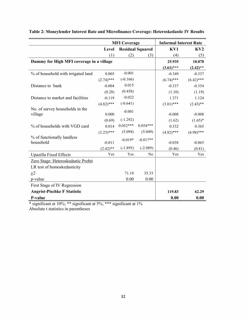
32

Table 2: Moneylender Interest Rate and Microfinance Coverage: Heteroskedastic IV Results

MFI Coverage Informal Interest Rate

Level Residual Squared KV1 KV2

(1) (2) (3) (4) (5) Dummy for High MFI coverage in a village

25.935 18.878

(3.61)*** (2.42)** % of household with irrigated land 0.005 -0.001 -0.349 -0.337

(2.74)*** (-0.166) (6.74)*** (6.42)***

Distance to bank -0.004 0.015 -0.337 -0.354

(0.28) (0.458) (1.10) (1.19)

Distance to market and facilities -0.119 -0.022 1.371 1.124

(4.82)*** (-0.641) (3.01)*** (2.43)**

No. of survey households in the village 0.000

-0.001 -0.008 -0.008

(0.69) (-1.292) (1.62) (1.65)*

% of households with VGD card 0.014 0.052*** 0.054*** 0.332 0.365

(3.25)*** (5.094) (5.049) (4.82)*** (4.98)***

% of functionally landless household -0.011

-0.019* -0.017** -0.038 -0.065

(2.42)** (-1.895) (-2.089) (0.46) (0.81) Upazilla Fixed Effects Yes Yes No Yes Yes

Zero Stage: Heteroskedastic Probit LR test of homoskedasticity

71.18 35.33

p-value 0.00 0.00 First Stage of IV Regression

Angrist-Pischke F Statistic

119.83 62.29 P-value 0.00 0.00

* significant at 10%; ** significant at 5%; *** significant at 1% Absolute t statistics in parentheses

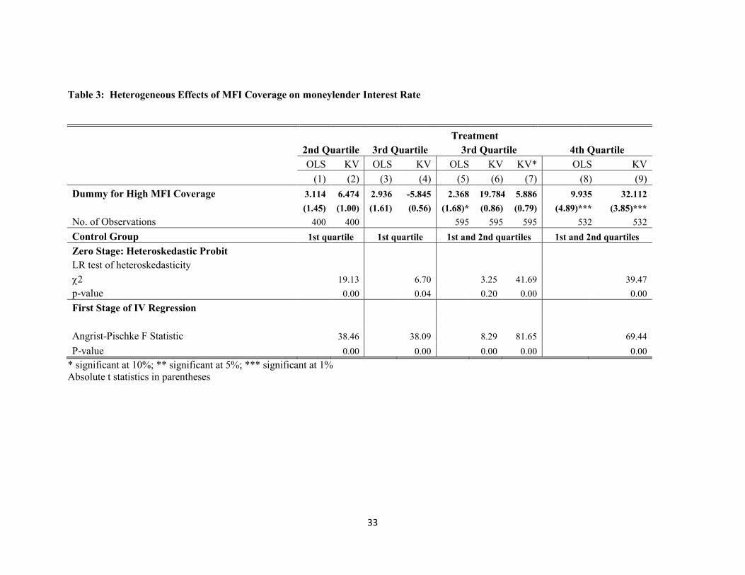
33

Table 3: Heterogeneous Effects of MFI Coverage on moneylender Interest Rate

Treatment

2nd Quartile 3rd Quartile 3rd Quartile 4th Quartile

OLS KV OLS KV OLS KV KV* OLS KV

(1) (2) (3) (4) (5) (6) (7) (8) (9) Dummy for High MFI Coverage 3.114 6.474 2.936 -5.845 2.368 19.784 5.886 9.935 32.112

(1.45) (1.00) (1.61) (0.56) (1.68)* (0.86) (0.79) (4.89)*** (3.85)***

No. of Observations 400 400 595 595 595 532 532 Control Group 1st quartile 1st quartile 1st and 2nd quartiles 1st and 2nd quartiles Zero Stage: Heteroskedastic Probit

LR test of heteroskedasticity

19.13

6.70

3.25 41.69

39.47

p-value 0.00 0.04 0.20 0.00 0.00 First Stage of IV Regression

Angrist-Pischke F Statistic

38.46

38.09

8.29 81.65

69.44

P-value 0.00 0.00 0.00 0.00 0.00 * significant at 10%; ** significant at 5%; *** significant at 1% Absolute t statistics in parentheses

34

Table 4: MFI Membership and Propensity to Borrow from Informal Sources

DID-FE MDID-FE MBDID-FE

(1) (2) (3) (4) (5) Control group: Never members

MFI member -0.041 -0.044 -0.047 -0.043 -0.065

(2.64)*** (2.76)*** (2.97)*** (3.09)*** (2.57)***

No. of Observations 1223 1223 1223 1223 1223 Control group: Dropouts

MFI member -0.059 -0.054 -0.053 -0.049 -0.083

(2.63)*** (2.39)** (2.34)** (1.82)* (2.20)***

No. of Observations 521 521 521 521 521 Control group: Never members & Dropouts

MFI member -0.044 -0.046 -0.049 -0.044 -0.059

(3.27)*** (2.90)*** (3.09)*** (3.32)*** (2.81)***

No. of Observations 1365 1365 1365 1365 1365 Household Controls No Yes Yes Yes Yes Region Controls No No Yes Yes Yes

* significant at 10%; ** significant at 5%; *** significant at 1% Absolute t statistics in parentheses.

Table 5: MFI membership and propensity to borrow from informal sources: Land-poor households (Less than 1 acre of agricultural land)

DID-FE MDID-FE MBDID-FE

(1) (2) (3) (4) (5) Control group: Never members

MFI member -0.045 -0.044 -0.050 -0.050 -0.061

(2.32)** (2.24)** (2.50)** (2.78)*** (1.70)*

No. of Observations 749 749 749 749 749

Control group: Dropouts MFI member -0.078 -0.074 -0.074 -0.074 -0.066

(2.72)*** (2.54)** (2.55)** (2.07)** (1.39)

No. of Observations 363 363 363 363 363 Control group: Never members & Dropouts

MFI member -0.050 -0.051 -0.056 -0.053 -0.055

(2.59)*** (2.55)** (2.83)*** (3.1)*** (1.73)*

No. of Observations 842 842 842 842 842

Household Controls No Yes Yes Yes Yes Region Controls No No Yes Yes Yes

* significant at 10%; ** significant at 5%; *** significant at 1% Absolute t statistics in parentheses

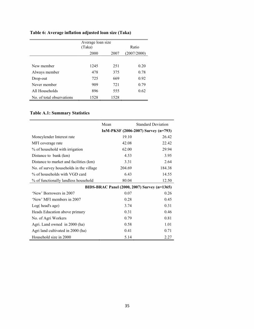
35

Table 6: Average inflation adjusted loan size (Taka)

Average loan size (Taka) Ratio

2000 2007 (2007/2000)

New member 1245 251 0.20 Always member 478 375 0.78 Drop-out 725 669 0.92 Never member 909 721 0.79 All Households 896 555 0.62 No. of total observations 1528 1528

Table A.1: Summary Statistics

Mean Standard Deviation

InM-PKSF (2006-2007) Survey (n=793)

Moneylender Interest rate 19.10 26.42 MFI coverage rate 42.08 22.42 % of household with irrigation 62.00 29.94 Distance to bank (km) 4.53 3.95 Distance to market and facilities (km) 3.31 2.64 No. of survey households in the village 204.69 184.38 % of households with VGD card 6.43 14.55 % of functionally landless household 80.04 12.50

BIDS-BRAC Panel (2000, 2007) Survey (n=1365) ‘New’ Borrowers in 2007 0.07 0.26 ‘New’ MFI members in 2007 0.28 0.45 Log( head's age) 3.74 0.31 Heads Education above primary 0.31 0.46 No. of Agri Workers 0.79 0.81 Agri. Land owned in 2000 (ha) 0.58 1.01 Agri land cultivated in 2000 (ha) 0.41 0.71 Household size in 2000 5.14 2.27

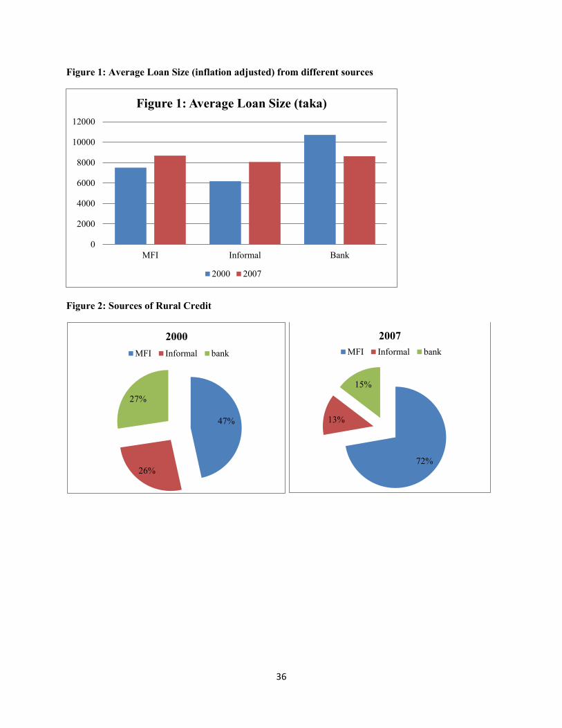
36

Figure 1: Average Loan Size (inflation adjusted) from different sources

Figure 2: Sources of Rural Credit

0

2000

4000

6000

8000

10000

12000

MFI Informal Bank

Figure 1: Average Loan Size (taka)

2000 2007

47%

26%

27%

2000 MFI Informal bank

72%

13%

15%

2007 MFI Informal bank