metrics guide 1
TRANSCRIPT

8/3/2019 Metrics Guide 1
http://slidepdf.com/reader/full/metrics-guide-1 1/29
Study Guide for Econometrics
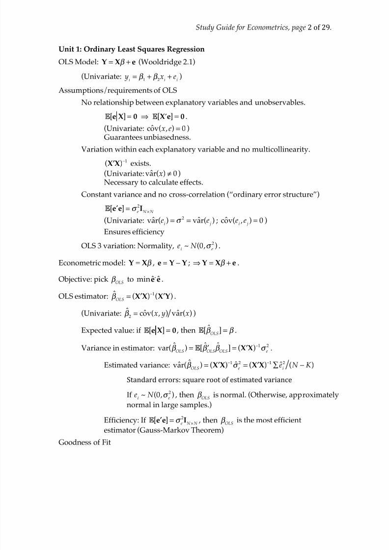
Unit 0: Preliminaries
Data types
Cross-sectional data
Time-series data
Panel data (or longitudinal data)
8/3/2019 Metrics Guide 1
http://slidepdf.com/reader/full/metrics-guide-1 2/29
8/3/2019 Metrics Guide 1
http://slidepdf.com/reader/full/metrics-guide-1 3/29
Study Guide for Econometrics, page 3of29.
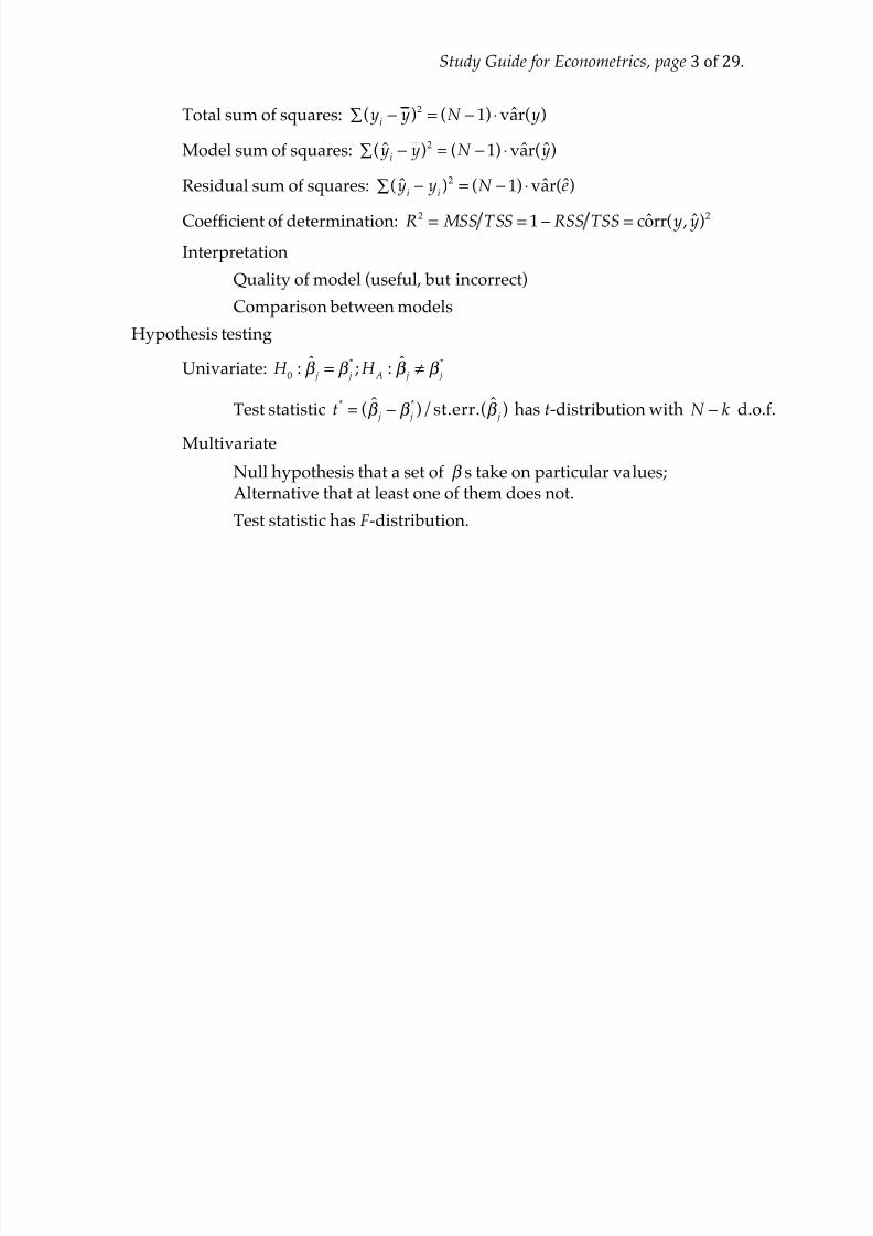
Total sum of squares: ( yi∑ − y)2 = (N − 1) ⋅var( y)
Model sum of squares: ( ˆ yi∑ − y)2 = (N −1) ⋅var( ˆ y)
Residual sum of squares: ( ˆ yi∑ − y
i)2 = (N − 1) ⋅var(e)
Coefficient of determination: R2 = MSS TSS = 1−RSS TSS = corr( y , ˆ y)2
Interpretation
Quality of model (useful, but incorrect)
Comparison between models
Hypothesis testing
Univariate: H 0: β
j =β j
*;H
A: β
j≠ β
j
*
Test statistic t*= (β j − β j
*)/st.err.(β j ) has t-distribution with N − k d.o.f.
Multivariate
Null hypothesis that a set of β s take on particular values;Alternative that at least one of them does not.
Test statistic has F-distribution.
8/3/2019 Metrics Guide 1
http://slidepdf.com/reader/full/metrics-guide-1 4/29
Study Guide for Econometrics, page 4of29.
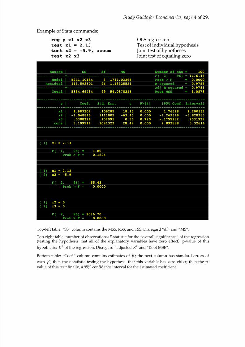
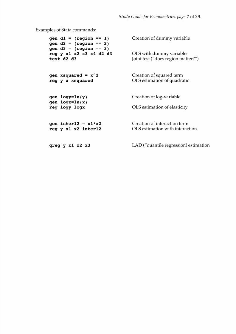
Example of Stata commands:
reg y x1 x2 x3 OLS regression test x1 = 2.13 Test of individual hypothesis test x2 = -5.9, accum Joint test of hypotheses test x2 x3 Joint test of equaling zero
. reg y x1 x2 x3
Source | SS df MS Number of obs = 100 -------------+------------------------------ F( 3, 96) = 1476.46
Model | 5241.10184 3 1747.03395 Prob > F = 0.0000 Residual | 113.592501 96 1.18325521 R-squared = 0.9788
-------------+------------------------------ Adj R-squared = 0.9781 Total | 5354.69434 99 54.0878216 Root MSE = 1.0878
------------------------------------------------------------------------------y | Coef. Std. Err. t P>|t| [95% Conf. Interval]
-------------+----------------------------------------------------------------x1 | 1.983209 .109285 18.15 0.000 1.76628 2.200137x2 | -7.048816 .1111005 -63.45 0.000 -7.269349 -6.828283x3 | .0388324 .107991 0.36 0.720 -.1755282 .2531929
_cons | 3.109514 .1091322 28.49 0.000 2.892888 3.32614------------------------------------------------------------------------------
. test x1 = 2.13
( 1) x1 = 2.13
F( 1, 96) = 1.80Prob > F = 0.1824
. test x2 = -5.9, accum
( 1) x1 = 2.13( 2) x2 = -5.9
F( 2, 96) = 55.42Prob > F = 0.0000
. test x2 x3
( 1) x2 = 0( 2) x3 = 0
F( 2, 96) = 2076.70Prob > F = 0.0000
Top-left table: “SS” column contains the MSS, RSS, and TSS. Disregard “df” and “MS”.
Top-right table: number of observations; F-statistic for the “overall significance” of the regression
(testing the hypothesis that all of the explanatory variables have zero effect); p-value of thishypothesis; R
2
of the regression. Disregard “adjusted R2
and “Root MSE”.
Bottom table: “Coef.” column contains estimates of β ; the next column has standard errors of
each β ; then the t-statistic testing the hypothesis that this variable has zero effect; then the p-value of this test; finally, a 95% confidence interval for the estimated coefficient.
8/3/2019 Metrics Guide 1
http://slidepdf.com/reader/full/metrics-guide-1 5/29
Study Guide for Econometrics, page 5of29.
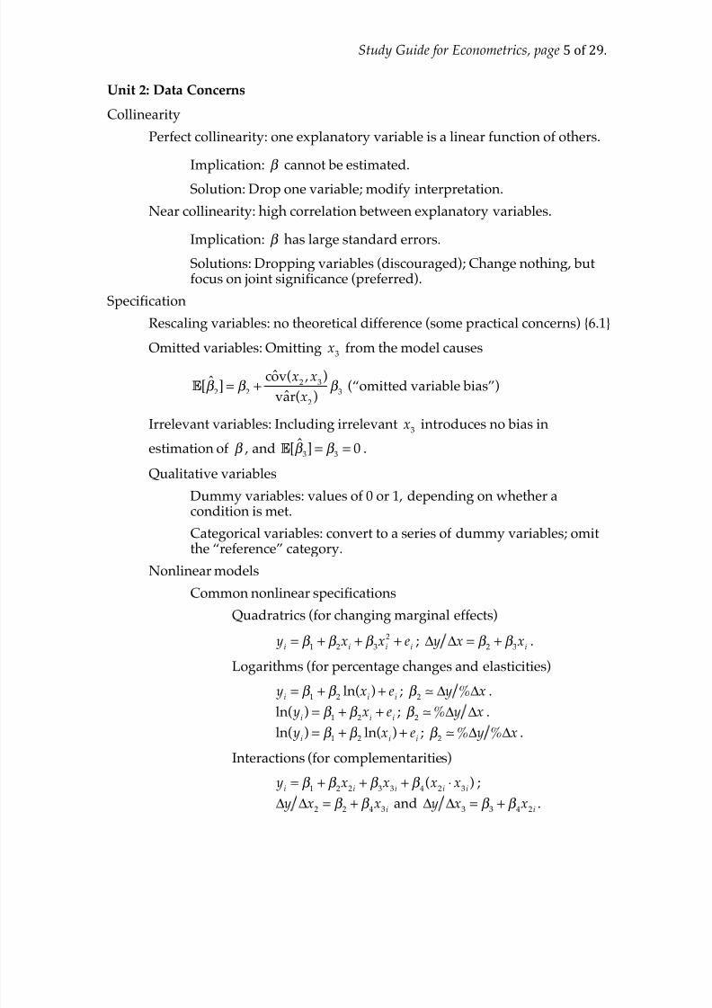
Unit 2: Data Concerns
Collinearity
Perfect collinearity: one explanatory variable is a linear function of others.
Implication: ˆβ cannot be estimated.
Solution: Drop one variable; modify interpretation.
Near collinearity: high correlation between explanatory variables.
Implication: ˆβ has large standard errors.
Solutions: Dropping variables (discouraged); Change nothing, butfocus on joint significance (preferred).
Specification
Rescaling variables: no theoretical difference (some practical concerns) {6.1}
Omitted variables: Omittingx3 from the model causes
E[β 2] = β
2+
cov(x2,x
3)
var(x2)
β 3
(“omitted variable bias”)
Irrelevant variables: Including irrelevant x3
introduces no bias in
estimation of β , and E[β 3] = β
3= 0 .
Qualitative variables
Dummy variables: values of 0 or 1, depending on whether acondition is met.
Categorical variables: convert to a series of dummy variables; omitthe “reference” category.
Nonlinear models
Common nonlinear specifications
Quadratrics (for changing marginal effects)
yi = β
1+ β
2x
i + β 3x
i
2+ e
i; Δ y Δx = β
2+ β
3x
i.
Logarithms (for percentage changes and elasticities)
yi =
β 1+ β
2ln(x
i)+ e
i; β
2 Δ y %Δx .
ln( yi ) = β 1 + β 2xi +ei ; β 2 %Δ y Δx .
ln( yi) = β
1+ β
2ln(x
i)+ e
i; β
2%Δ y %Δx .
Interactions (for complementarities)
yi =
β 1+ β
2x
2 i +β
3x
3 i +β
4(x
2 i⋅ x
3 i) ;
Δ y Δx2= β
2+ β
4x3i
and Δ y Δx3= β
3+ β
4x2i
.
8/3/2019 Metrics Guide 1
http://slidepdf.com/reader/full/metrics-guide-1 6/29
Study Guide for Econometrics, page 6of29.
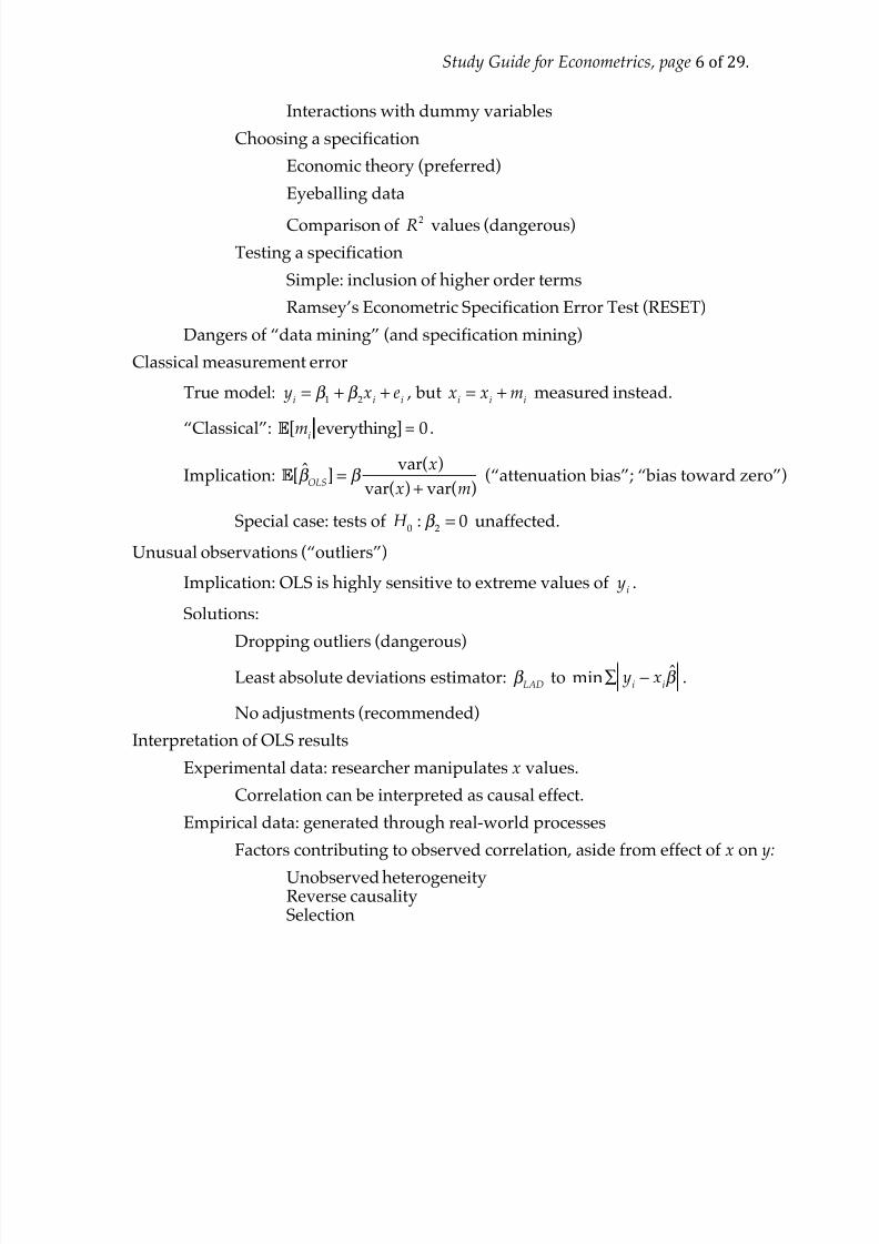
Interactions with dummy variables
Choosing a specification
Economic theory (preferred)
Eyeballing data
Comparison of R2 values (dangerous)
Testing a specification
Simple: inclusion of higher order terms
Ramsey’s Econometric Specification Error Test (RESET)
Dangers of “data mining” (and specification mining)
Classical measurement error
True model: yi= β
1+ β
2x
i+ e
i , but x
i= x
i+m
imeasured instead.
“Classical”:E
[m
i everything]=
0 .
Implication: E[β OLS
] = β var(x)
var(x)+ var(m)(“attenuation bias”; “bias toward zero”)
Special case: tests of H 0: β
2= 0 unaffected.
Unusual observations (“outliers”)
Implication: OLS is highly sensitive to extreme values of yi.
Solutions:
Dropping outliers (dangerous)
Least absolute deviations estimator: ˆβ LAD
to min∑ yi− x
iβ .
No adjustments (recommended)
Interpretation of OLS results
Experimental data: researcher manipulates x values.
Correlation can be interpreted as causal effect.
Empirical data: generated through real-world processes
Factors contributing to observed correlation, aside from effect of x on y:
Unobserved heterogeneityReverse causalitySelection
8/3/2019 Metrics Guide 1
http://slidepdf.com/reader/full/metrics-guide-1 7/29
8/3/2019 Metrics Guide 1
http://slidepdf.com/reader/full/metrics-guide-1 8/29
Study Guide for Econometrics, page 8of29.
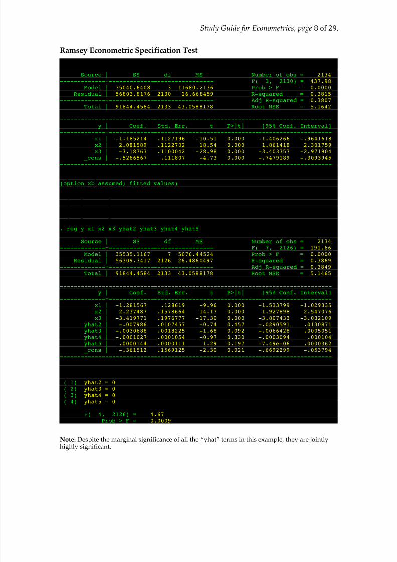
Ramsey Econometric Specification Test
. reg y x1 x2 x3
Source | SS df MS Number of obs = 2134-------------+------------------------------ F( 3, 2130) = 437.98
Model | 35040.6408 3 11680.2136 Prob > F = 0.0000Residual | 56803.8176 2130 26.668459 R-squared = 0.3815
-------------+------------------------------ Adj R-squared = 0.3807Total | 91844.4584 2133 43.0588178 Root MSE = 5.1642
------------------------------------------------------------------------------y | Coef. Std. Err. t P>|t| [95% Conf. Interval]
-------------+----------------------------------------------------------------x1 | -1.185214 .1127196 -10.51 0.000 -1.406266 -.9641618 x2 | 2.081589 .1122702 18.54 0.000 1.861418 2.301759 x3 | -3.18763 .1100042 -28.98 0.000 -3.403357 -2.971904
_cons | -.5286567 .111807 -4.73 0.000 -.7479189 -.3093945 ------------------------------------------------------------------------------
. predict yhat(option xb assumed; fitted values)
. gen yhat2 = yhat^2
. gen yhat3 = yhat^3
. gen yhat4 = yhat^4
. gen yhat5 = yhat^5
. reg y x1 x2 x3 yhat2 yhat3 yhat4 yhat5
Source | SS df MS Number of obs = 2134-------------+------------------------------ F( 7, 2126) = 191.66
Model | 35535.1167 7 5076.44524 Prob > F = 0.0000Residual | 56309.3417 2126 26.4860497 R-squared = 0.3869
-------------+------------------------------ Adj R-squared = 0.3849Total | 91844.4584 2133 43.0588178 Root MSE = 5.1465
------------------------------------------------------------------------------
y | Coef. Std. Err. t P>|t| [95% Conf. Interval]-------------+----------------------------------------------------------------x1 | -1.281567 .128619 -9.96 0.000 -1.533799 -1.029335 x2 | 2.237487 .1578664 14.17 0.000 1.927898 2.547076 x3 | -3.419771 .1976777 -17.30 0.000 -3.807433 -3.032109
yhat2 | -.007986 .0107457 -0.74 0.457 -.0290591 .0130871 yhat3 | -.0030688 .0018225 -1.68 0.092 -.0066428 .0005051 yhat4 | -.0001027 .0001054 -0.97 0.330 -.0003094 .000104 yhat5 | .0000144 .0000111 1.29 0.197 -7.49e-06 .0000362 _cons | -.361512 .1569125 -2.30 0.021 -.6692299 -.053794
------------------------------------------------------------------------------
. test yhat2 yhat3 yhat4 yhat5
( 1) yhat2 = 0 ( 2) yhat3 = 0
( 3) yhat4 = 0 ( 4) yhat5 = 0
F( 4, 2126) = 4.67 Prob > F = 0.0009
Note: Despite the marginal significance of all the “yhat” terms in this example, they are jointlyhighly significant.
8/3/2019 Metrics Guide 1
http://slidepdf.com/reader/full/metrics-guide-1 9/29
Study Guide for Econometrics, page 9of29.
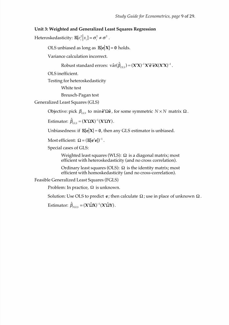
Unit 3: Weighted and Generalized Least Squares Regression
Heteroskedasticity: E[ei
2x
i] = σ
i
2≠ σ
2 .
OLS unbiased as long as E[e X] = 0 holds.
Variance calculation incorrect.
Robust standard errors: var(β OLS
) = ( ′X X)−1 ′X ˆ′e eX( ′X X)−1 .
OLS inefficient.
Testing for heteroskedasticity
White test
Breusch-Pagan test
Generalized Least Squares (GLS)
Objective: pick
ˆβ GLS to
min ˆ′e Ωe
, for some symmetricN × N
matrixΩ
.Estimator: β
GLS= ( ′X ΩX)−1( ′X ΩY) .
Unbiasedness: if E[e X] = 0 , then any GLS estimator is unbiased.
Most efficient: Ω = (E[ ′e e])−1 .
Special cases of GLS:
Weighted least squares (WLS): Ω is a diagonal matrix; mostefficient with heteroskedasticity (and no cross correlation).
Ordinary least squares (OLS): Ω is the identity matrix; mostefficient with homoskedasticity (and no cross-correlation).
Feasible Generalized Least Squares (FGLS)
Problem: In practice, Ω is unknown.
Solution: Use OLS to predict e ; then calculate ˆΩ ; use in place of unknown Ω .
Estimator: β FGLS
= ( ′X ΩX)−1( ′X ΩY) .
8/3/2019 Metrics Guide 1
http://slidepdf.com/reader/full/metrics-guide-1 10/29
Study Guide for Econometrics, page 10of29.
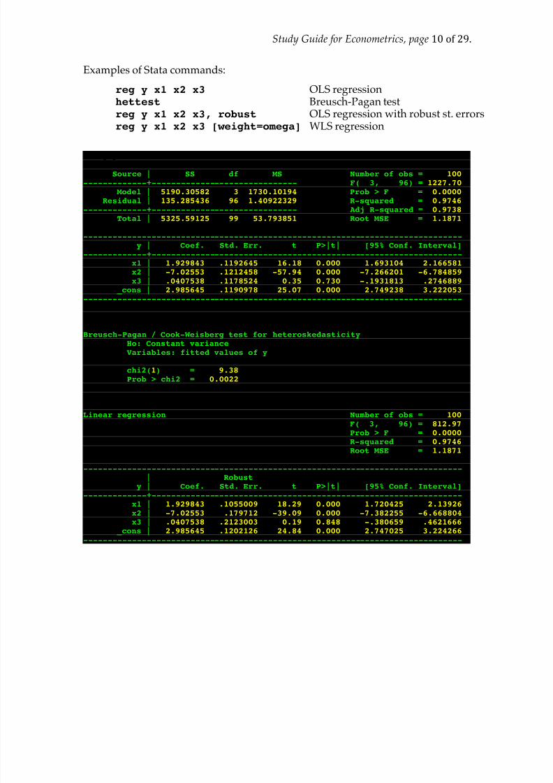
Examples of Stata commands:
reg y x1 x2 x3 OLS regression hettest Breusch-Pagan test reg y x1 x2 x3, robust OLS regression with robust st. errors reg y x1 x2 x3 [weight=omega] WLS regression
. reg y x1 x2 x3
Source | SS df MS Number of obs = 100 -------------+------------------------------ F( 3, 96) = 1227.70
Model | 5190.30582 3 1730.10194 Prob > F = 0.0000 Residual | 135.285436 96 1.40922329 R-squared = 0.9746
-------------+------------------------------ Adj R-squared = 0.9738 Total | 5325.59125 99 53.793851 Root MSE = 1.1871
------------------------------------------------------------------------------y | Coef. Std. Err. t P>|t| [95% Conf. Interval]
-------------+----------------------------------------------------------------x1 | 1.929843 .1192645 16.18 0.000 1.693104 2.166581
x2 | -7.02553 .1212458 -57.94 0.000 -7.266201 -6.784859x3 | .0407538 .1178524 0.35 0.730 -.1931813 .2746889 _cons | 2.985645 .1190978 25.07 0.000 2.749238 3.222053
------------------------------------------------------------------------------
. hettest
Breusch-Pagan / Cook-Weisberg test for heteroskedasticityHo: Constant varianceVariables: fitted values of y
chi2(1) = 9.38Prob > chi2 = 0.0022
. reg y x1 x2 x3, robust
Linear regression Number of obs = 100 F( 3, 96) = 812.97 Prob > F = 0.0000 R-squared = 0.9746 Root MSE = 1.1871
------------------------------------------------------------------------------| Robust
y | Coef. Std. Err. t P>|t| [95% Conf. Interval]-------------+----------------------------------------------------------------
x1 | 1.929843 .1055009 18.29 0.000 1.720425 2.13926x2 | -7.02553 .179712 -39.09 0.000 -7.382255 -6.668804x3 | .0407538 .2123003 0.19 0.848 -.380659 .4621666
_cons | 2.985645 .1202126 24.84 0.000 2.747025 3.224266------------------------------------------------------------------------------
8/3/2019 Metrics Guide 1
http://slidepdf.com/reader/full/metrics-guide-1 11/29
Study Guide for Econometrics, page 11of29.
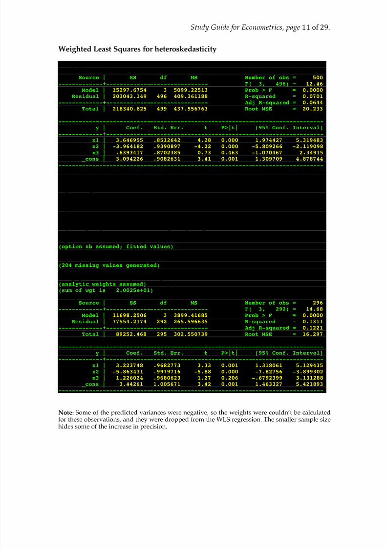
Weighted Least Squares for heteroskedasticity
. reg y x1 x2 x3
Source | SS df MS Number of obs = 500-------------+------------------------------ F( 3, 496) = 12.46
Model | 15297.6754 3 5099.22513 Prob > F = 0.0000
Residual | 203043.149 496 409.361188 R-squared = 0.0701-------------+------------------------------ Adj R-squared = 0.0644
Total | 218340.825 499 437.556763 Root MSE = 20.233
------------------------------------------------------------------------------y | Coef. Std. Err. t P>|t| [95% Conf. Interval]
-------------+----------------------------------------------------------------x1 | 3.646955 .8512642 4.28 0.000 1.974427 5.319483x2 | -3.964182 .9390897 -4.22 0.000 -5.809266 -2.119098x3 | .6393417 .8702385 0.73 0.463 -1.070467 2.34915
_cons | 3.094226 .9082631 3.41 0.001 1.309709 4.878744------------------------------------------------------------------------------
. predict ehat, resid
. gen ehat2 = ehat^2
. gen x1sq = x1^2. gen x2sq = x2^2
. gen x3sq = x3^2
. gen x1x2 = x1*x2
. gen x1x3 = x1*x3
. gen x2x3 = x2*x3
. quietly reg ehat2 x1 x2 x3 x1sq x2sq x3sq x1x2 x1x3 x2x3
. predict ehat2hat(option xb assumed; fitted values)
. gen omega = 1/(ehat2hat)^.5(204 missing values generated)
. reg y x1 x2 x3 [weight = omega](analytic weights assumed)
(sum of wgt is 2.0025e+01)
Source | SS df MS Number of obs = 296-------------+------------------------------ F( 3, 292) = 14.68
Model | 11698.2506 3 3899.41685 Prob > F = 0.0000Residual | 77554.2174 292 265.596635 R-squared = 0.1311
-------------+------------------------------ Adj R-squared = 0.1221Total | 89252.468 295 302.550739 Root MSE = 16.297
------------------------------------------------------------------------------y | Coef. Std. Err. t P>|t| [95% Conf. Interval]
-------------+----------------------------------------------------------------x1 | 3.223748 .9682773 3.33 0.001 1.318061 5.129435x2 | -5.863431 .9979716 -5.88 0.000 -7.82756 -3.899302x3 | 1.226024 .9680623 1.27 0.206 -.6792399 3.131288
_cons | 3.44261 1.005671 3.42 0.001 1.463327 5.421893------------------------------------------------------------------------------
Note: Some of the predicted variances were negative, so the weights were couldn’t be calculatedfor these observations, and they were dropped from the WLS regression. The smaller sample sizehides some of the increase in precision.
8/3/2019 Metrics Guide 1
http://slidepdf.com/reader/full/metrics-guide-1 12/29
Study Guide for Econometrics, page 12of29.
Unit 4: Instrumental Variables Regression
Endogeneity: E[e X] ≠ 0 .
OLS with endogenous regressors: E[β OLS
] = β + ( ′X X)−1( ′X e) ; biased.
Instrumental variable: has ability to predict endogenous regressors.Assumptions/requirements for the instrument:
At least as many instruments as explanatory variables; #Z ≥#X .
Note: if x j
is exogenous, it is technically used as an instrument for itself.
Uncorrelated with unobservables; E[e Z] = 0 ⇒ E[ ′Z e] = 0 ( E[e X] ≠ 0
usually, but not necessarily.)
Correlated with the endogenous explanatory variables; ( ′Z X) is invertible,when same number of instruments. (Generally: ( ′Z X) is of full rank.)
Two-Stage Least Squares (2SLS)
First stage: X = Zγ + u ⇒ γ = ( ′Z Z)−1( ′Z X) ⇒ ˆX = Zγ .
Second stage: regression of Y on ˆX yields β 2SLS
= ( ˆ ′X X)−1( ˆ ′X Y)
(Standard errors incorrect)
Instrumental Variables Regression: direct computation
β 2SLS =
( ˆ ′X X)−1( ˆ ′X Y) is equivalent to ( ′Z X)−1( ′Z Y) = β IV
(when #Z =#X )
Variance in estimator:
Estimated variance: var(β IV ) = ( ′Z X)
−1( ′Z Z)( ′X Z)−1σ
e
2
Inefficiency: var(β IV ) =
var(β OLS
)
corr(x ,z)2 , when #X =#Z = 1 .
Post-estimation tests
Hausman test: explanatory variables are endogenous.
Motivation: because of efficiency, OLS is preferred to IV if no endogeneity.
Null hypothesis: E[β IV
] = β = E[β OLS
] , var[β IV ] ≥ var[β
OLS] .
Alternative hypothesis: E[β IV
] = β .
Check for weak instruments: cov(x ,z) ≈ 0 ?
Motivation: with weak instruments, very inefficient; biases get magnified;also, distribution of estimator may not be approximately normal.
Correlations; F-statistics from first stage.
8/3/2019 Metrics Guide 1
http://slidepdf.com/reader/full/metrics-guide-1 13/29
8/3/2019 Metrics Guide 1
http://slidepdf.com/reader/full/metrics-guide-1 14/29
Study Guide for Econometrics, page 14of29.
Examples of Stata commands:
IV regression: x1 and x2 are exogenous, x3 and x4 are endogenous, and z1 , z2 ,and z3 (plus x1 and x2) are instruments.
ivreg y x1 x2 (x3 x4 = z1 z2 z3)
IV regression, displaying first-stage results.ivreg y x1 x2 (x3 x4 = z1 z2 z3), first
Hausman test
ivreg y x1 x2 (x3 x4 = z1 z2 z3) est sto ivest reg y x1 x2 x3 x4 est sto olsest hausman ivest olsest
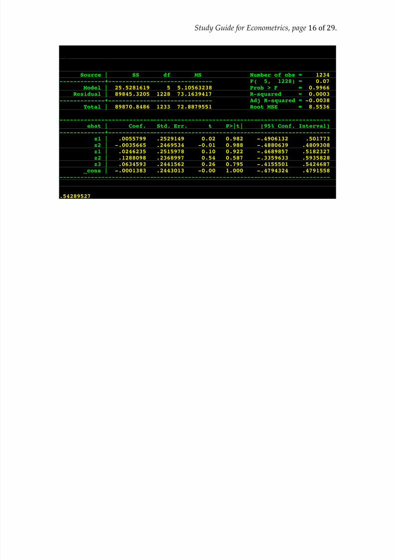
Test of over-identification
ivreg y x1 x2 (x3 x4 = z1 z2 z3) predict ehat, residreg ehat x1 x2 z1 z2 z3
8/3/2019 Metrics Guide 1
http://slidepdf.com/reader/full/metrics-guide-1 15/29
Study Guide for Econometrics, page 15of29.
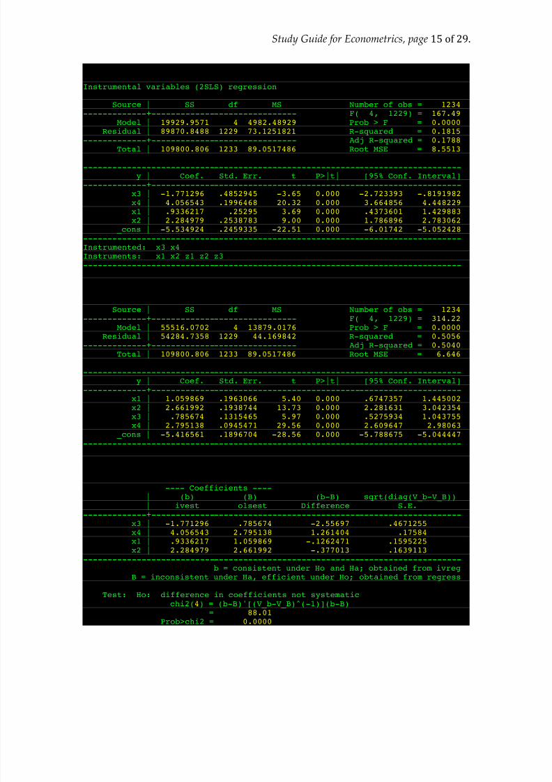
. ivreg y x1 x2 (x3 x4 = z1 z2 z3)
Instrumental variables (2SLS) regression
Source | SS df MS Number of obs = 1234 -------------+------------------------------ F( 4, 1229) = 167.49
Model | 19929.9571 4 4982.48929 Prob > F = 0.0000 Residual | 89870.8488 1229 73.1251821 R-squared = 0.1815
-------------+------------------------------ Adj R-squared = 0.1788 Total | 109800.806 1233 89.0517486 Root MSE = 8.5513
------------------------------------------------------------------------------y | Coef. Std. Err. t P>|t| [95% Conf. Interval]
-------------+----------------------------------------------------------------x3 | -1.771296 .4852945 -3.65 0.000 -2.723393 -.8191982x4 | 4.056543 .1996468 20.32 0.000 3.664856 4.448229x1 | .9336217 .25295 3.69 0.000 .4373601 1.429883x2 | 2.284979 .2538783 9.00 0.000 1.786896 2.783062
_cons | -5.534924 .2459335 -22.51 0.000 -6.01742 -5.052428------------------------------------------------------------------------------Instrumented: x3 x4Instruments: x1 x2 z1 z2 z3------------------------------------------------------------------------------
. est sto ivest
. reg y x1 x2 x3 x4
Source | SS df MS Number of obs = 1234-------------+------------------------------ F( 4, 1229) = 314.22
Model | 55516.0702 4 13879.0176 Prob > F = 0.0000Residual | 54284.7358 1229 44.169842 R-squared = 0.5056
-------------+------------------------------ Adj R-squared = 0.5040Total | 109800.806 1233 89.0517486 Root MSE = 6.646
------------------------------------------------------------------------------y | Coef. Std. Err. t P>|t| [95% Conf. Interval]
-------------+----------------------------------------------------------------x1 | 1.059869 .1963066 5.40 0.000 .6747357 1.445002
x2 | 2.661992 .1938744 13.73 0.000 2.281631 3.042354x3 | .785674 .1315465 5.97 0.000 .5275934 1.043755x4 | 2.795138 .0945471 29.56 0.000 2.609647 2.98063
_cons | -5.416561 .1896704 -28.56 0.000 -5.788675 -5.044447------------------------------------------------------------------------------
. est sto olsest
. hausman ivest olsest
---- Coefficients ----| (b) (B) (b-B) sqrt(diag(V_b-V_B))| ivest olsest Difference S.E.
-------------+----------------------------------------------------------------x3 | -1.771296 .785674 -2.55697 .4671255 x4 | 4.056543 2.795138 1.261404 .17584 x1 | .9336217 1.059869 -.1262471 .1595225
x2 | 2.284979 2.661992 -.377013 .1639113 ------------------------------------------------------------------------------
b = consistent under Ho and Ha; obtained from ivregB = inconsistent under Ha, efficient under Ho; obtained from regress
Test: Ho: difference in coefficients not systematicchi2(4) = (b-B)'[(V_b-V_B)^(-1)](b-B)
= 88.01Prob>chi2 = 0.0000
8/3/2019 Metrics Guide 1
http://slidepdf.com/reader/full/metrics-guide-1 16/29
8/3/2019 Metrics Guide 1
http://slidepdf.com/reader/full/metrics-guide-1 17/29
Study Guide for Econometrics, page 17of29.
Unit 5: Systems of Equations
Endogenous: the value of yi
is determined in part by other variables in the system.
Exogenous: the value of xi
is determined by unrelated, outside forces.
Simultaneity bias
Model: y1i = β
1+ β
2 y
2i +…; y
2i = γ 1+ γ
2 y
1i +…
OLS estimates of β and γ are biased.
2SLS for systems of equations with endogenous regressors
Model: y1i =
β 1+ β
2 y
2 i +β 3x1i +
β 4x2i +
e1i
; y2i = γ
1+ γ
2 y
1i + γ 3x1i + γ
4x3i +
e2i.
Someoverlapinexogenousexplanatoryvariables.
Someendogenousvariablesarepredictorsofothers.
Twoormoreequations.
Assumptions: all x variables are exogenous.
“Identification”: to measure the effect of yi
on other outcomes, musthave one variable in this equation that does not appear in others.
Technique:
1. Regress each endogenous explanatory variable yi
on its
exogenous determinants; obtain predicted values, ˆ yi
.
2. Regress each outcome on its exogenous explanatorydeterminants and the predicted values of the endogenous variables.
Note: incorrect standard errors.
Inefficiency: does not take advantage of correlation between anindividual’s unobservables in different equations.
Seemingly Unrelated Regression (SUR) for systems with exogenous regressors
Model: y1i= x
1iβ 1+ e
1i; y
2i= x
2 iβ 2+ e
2i; etc.
Some (or complete) overlap in explanatory variables.
Two or more equations.
OLS estimation of each equation separately is unbiased, but inefficient.
Motivation for SUR: accounting for cross-equation correlation inunobservables can yield more precise estimates.
Technique: FGLS.
3SLS for systems of equations with endogenous regressors
Model: y1i= β
1+ β
2 y
2 i+ β
3x1i+ β
4x2i+ e
1i; y
2i= γ
1+ γ
2 y
1i+ γ
3x1i+ γ
4x3i+ e
2i.
Someoverlapinexogenousexplanatoryvariables.

8/3/2019 Metrics Guide 1
http://slidepdf.com/reader/full/metrics-guide-1 18/29
Study Guide for Econometrics, page 18of29.
Someendogenousvariablesarepredictorsofothers.
Twoormoreequations.
Motivation: Correct for simultaneity bias, plus improve precision.
Technique: 2SLS combined with FGLS.
“Identification”: to measure the effect of yi
on other outcomes, must haveone variable in this equation that does not appear in others.
Efficiency: most efficient estimator.
8/3/2019 Metrics Guide 1
http://slidepdf.com/reader/full/metrics-guide-1 19/29
Study Guide for Econometrics, page 19of29.
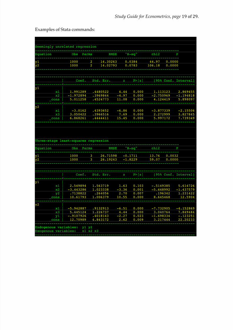
Examples of Stata commands:
. reg3 (y1 = x1 x2) (y2 = x1 x3), sur
Seemingly unrelated regression----------------------------------------------------------------------Equation Obs Parms RMSE "R-sq" chi2 P
----------------------------------------------------------------------y1 1000 2 14.30263 0.0384 44.97 0.0000y2 1000 2 14.02793 0.0783 106.18 0.0000----------------------------------------------------------------------
------------------------------------------------------------------------------| Coef. Std. Err. z P>|z| [95% Conf. Interval]
-------------+----------------------------------------------------------------y1 |
x1 | 1.991289 .4480522 4.44 0.000 1.113123 2.869455x2 | -1.972894 .3969844 -4.97 0.000 -2.750969 -1.194818
_cons | 5.011258 .4524773 11.08 0.000 4.124419 5.898097-------------+----------------------------------------------------------------y2 |
x1 | -3.0162 .4393652 -6.86 0.000 -3.877339 -2.15506
x3 | 3.050422 .3966516 7.69 0.000 2.272999 3.827845 _cons | 6.868261 .4444411 15.45 0.000 5.997172 7.739349------------------------------------------------------------------------------
. reg3 (y1 = x1 x2 y2) (y2 = x1 x3 y1)
Three-stage least-squares regression----------------------------------------------------------------------Equation Obs Parms RMSE "R-sq" chi2 P----------------------------------------------------------------------y1 1000 3 26.71598 -0.1711 13.76 0.0032y2 1000 3 26.19243 -1.8229 59.07 0.0000----------------------------------------------------------------------
------------------------------------------------------------------------------
| Coef. Std. Err. z P>|z| [95% Conf. Interval]-------------+----------------------------------------------------------------y1 |
x1 | 2.549894 1.563719 1.63 0.103 -.5149385 5.614726x2 | -3.443286 1.023338 -3.36 0.001 -5.448992 -1.437579y2 | .7138822 .264056 2.70 0.007 .196342 1.231422
_cons | 10.61793 1.006379 10.55 0.000 8.645468 12.5904-------------+----------------------------------------------------------------y2 |
x1 | -5.942887 .9132913 -6.51 0.000 -7.732905 -4.152869x3 | 5.445124 1.226737 4.44 0.000 3.040764 7.849484y1 | -.9107926 .4018143 -2.27 0.023 -1.698334 -.123251
_cons | 12.70989 4.843172 2.62 0.009 3.217444 22.20233------------------------------------------------------------------------------Endogenous variables: y1 y2
Exogenous variables: x1 x2 x3------------------------------------------------------------------------------

8/3/2019 Metrics Guide 1
http://slidepdf.com/reader/full/metrics-guide-1 20/29
Study Guide for Econometrics, page 20of29.
Unit 6: Policy Analysis
Before-and-after comparisons
Advantages: simplicity
Disadvantage: natural history, natural trend.
Controlling for effects of time
Difference-in-Difference estimation
“Counterfactual”
Natural experiments
Exogeneity requirements
Criticisms
Serial correlation
Exogeneity of policy
8/3/2019 Metrics Guide 1
http://slidepdf.com/reader/full/metrics-guide-1 21/29
Study Guide for Econometrics, page 21of29.
Unit 7: Panel Data Models
Panel data model: yit =
xitβ + e
it; e
it= c
i+ u
it.
Repeated observations of same individuals over time.
Permanent component and transitory component to unobservable.
Strict exogeneity: E[uitx
is] = 0 .
Error structure: E[ ′eie
i] = I
T ×T σ
u
2+ 1
T ×T σ
c
2 .
Pooled OLS (POLS): treats all observations as if from distinct individuals.
Unbiased if E[eit
xit] = 0 ; requires strict exogeneity and E[c
ix
it] = 0 .
Variance calculation incorrect
“Clustered” standard errors
Inefficient, because of cross-correlation between unobservables.
Random effects (RE): GLS with ΩRE
−1= E[ ′e
iei] = I
T ×T σ
u
2+ 1
T ×T σ
c
2 .
Estimator: β RE = ( ′X ΩREX)−1( ′X Ω
REY) .
Unbiased if E[eit
xit] = 0 ; requires strict exogeneity and E[c
ix
it] = 0 .
Most precise.
Fixed effects: OLS with transformed data.
Fixed effects transformation: xit
FE= x
it− x
i , y
it = y
it− y .
Estimator: β FE = ( ′X X)−1( ′X Y) .
Unbiased if E[eit
xit] = 0 ; requires only strict exogeneity.
Possibly inefficient.
First differences: OLS with differenced data.
Fixed effects transformation: Δxit= x
it− x
it−1 , Δ y
it = y
it− y
it−1.
Estimator: β FD= (Δ ′X ΔX)−1(Δ ′X ΔY) .
Unbiased if E[ΔeitΔx
it] = 0 ; requires (less than) strict exogeneity.
Possibly inefficient.
Dummy variables: OLS with a dummy variable for each individual.
Equivalent to Fixed Effects.
Relaxation of strict exogeneity

8/3/2019 Metrics Guide 1
http://slidepdf.com/reader/full/metrics-guide-1 22/29
8/3/2019 Metrics Guide 1
http://slidepdf.com/reader/full/metrics-guide-1 23/29
Study Guide for Econometrics, page 23of29.
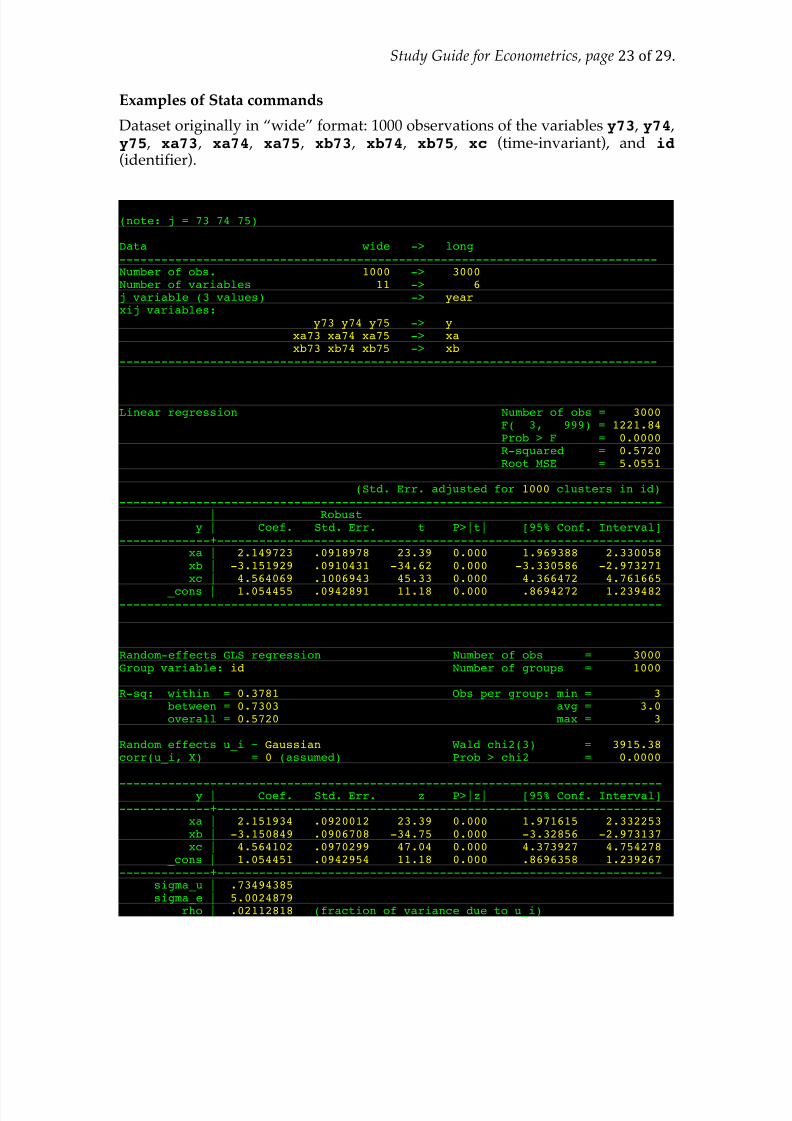
Examples of Stata commands
Dataset originally in “wide” format: 1000 observations of the variables y73 , y74 ,y75 , xa73 , xa74 , xa75 , xb73 , xb74 , xb75 , xc (time-invariant), and id (identifier).
. reshape long y xa xb, i(id) j(year)(note: j = 73 74 75)
Data wide -> long-----------------------------------------------------------------------------Number of obs. 1000 -> 3000 Number of variables 11 -> 6 j variable (3 values) -> year xij variables:
y73 y74 y75 -> y xa73 xa74 xa75 -> xa xb73 xb74 xb75 -> xb
-----------------------------------------------------------------------------
. reg y xa xb xc, cluster(id)Linear regression Number of obs = 3000
F( 3, 999) = 1221.84 Prob > F = 0.0000 R-squared = 0.5720 Root MSE = 5.0551
(Std. Err. adjusted for 1000 clusters in id)------------------------------------------------------------------------------
| Robusty | Coef. Std. Err. t P>|t| [95% Conf. Interval]
-------------+----------------------------------------------------------------xa | 2.149723 .0918978 23.39 0.000 1.969388 2.330058xb | -3.151929 .0910431 -34.62 0.000 -3.330586 -2.973271xc | 4.564069 .1006943 45.33 0.000 4.366472 4.761665
_cons | 1.054455 .0942891 11.18 0.000 .8694272 1.239482------------------------------------------------------------------------------
. xtreg y xa xb xc, re i(id)
Random-effects GLS regression Number of obs = 3000Group variable: id Number of groups = 1000
R-sq: within = 0.3781 Obs per group: min = 3between = 0.7303 avg = 3.0overall = 0.5720 max = 3
Random effects u_i ~ Gaussian Wald chi2(3) = 3915.38corr(u_i, X) = 0 (assumed) Prob > chi2 = 0.0000
------------------------------------------------------------------------------y | Coef. Std. Err. z P>|z| [95% Conf. Interval]-------------+----------------------------------------------------------------
xa | 2.151934 .0920012 23.39 0.000 1.971615 2.332253xb | -3.150849 .0906708 -34.75 0.000 -3.32856 -2.973137xc | 4.564102 .0970299 47.04 0.000 4.373927 4.754278
_cons | 1.054451 .0942954 11.18 0.000 .8696358 1.239267-------------+----------------------------------------------------------------
sigma_u | .73494385 sigma_e | 5.0024879
rho | .02112818 (fraction of variance due to u_i)
8/3/2019 Metrics Guide 1
http://slidepdf.com/reader/full/metrics-guide-1 24/29
Study Guide for Econometrics, page 24of29.
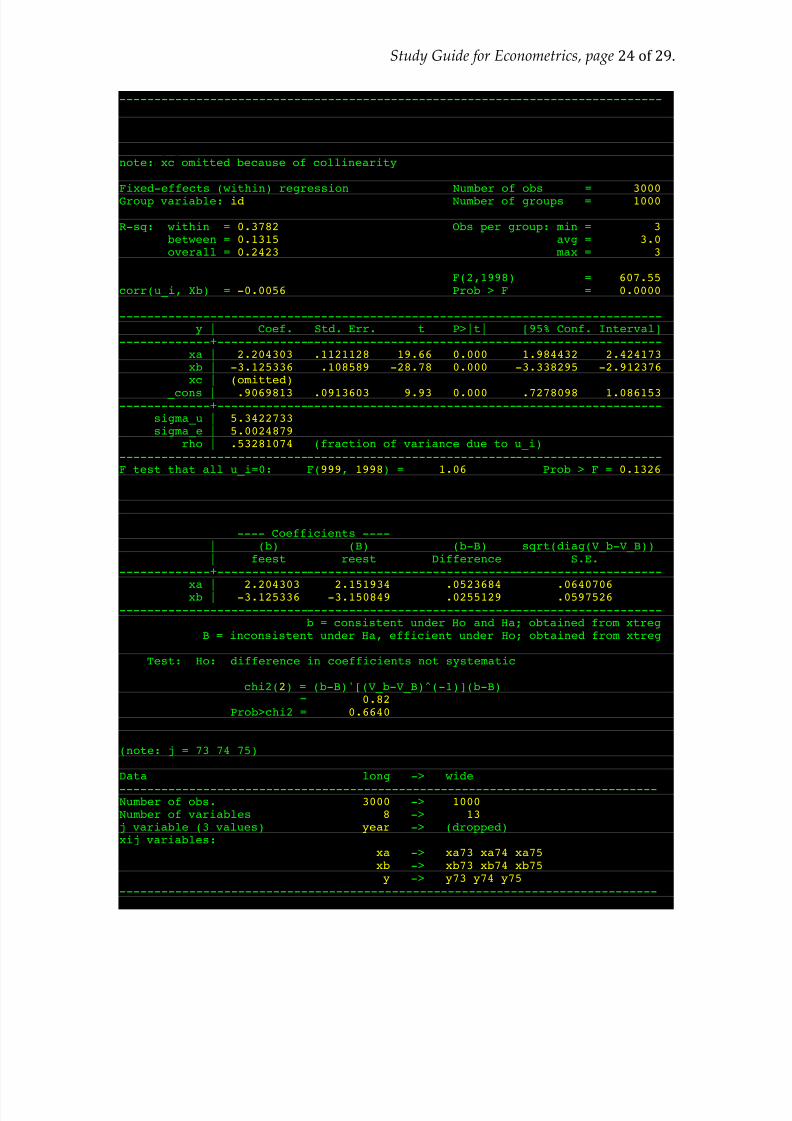
------------------------------------------------------------------------------
. est sto reest
. xtreg y xa xb xc, fe i(id)note: xc omitted because of collinearity
Fixed-effects (within) regression Number of obs = 3000Group variable: id Number of groups = 1000
R-sq: within = 0.3782 Obs per group: min = 3between = 0.1315 avg = 3.0overall = 0.2423 max = 3
F(2,1998) = 607.55corr(u_i, Xb) = -0.0056 Prob > F = 0.0000
------------------------------------------------------------------------------y | Coef. Std. Err. t P>|t| [95% Conf. Interval]
-------------+----------------------------------------------------------------xa | 2.204303 .1121128 19.66 0.000 1.984432 2.424173 xb | -3.125336 .108589 -28.78 0.000 -3.338295 -2.912376 xc | (omitted)
_cons | .9069813 .0913603 9.93 0.000 .7278098 1.086153 -------------+----------------------------------------------------------------
sigma_u | 5.3422733 sigma_e | 5.0024879
rho | .53281074 (fraction of variance due to u_i)------------------------------------------------------------------------------F test that all u_i=0: F(999, 1998) = 1.06 Prob > F = 0.1326
. est sto feest
. hausman feest reest
---- Coefficients ----| (b) (B) (b-B) sqrt(diag(V_b-V_B))| feest reest Difference S.E.
-------------+----------------------------------------------------------------
xa | 2.204303 2.151934 .0523684 .0640706 xb | -3.125336 -3.150849 .0255129 .0597526 ------------------------------------------------------------------------------
b = consistent under Ho and Ha; obtained from xtregB = inconsistent under Ha, efficient under Ho; obtained from xtreg
Test: Ho: difference in coefficients not systematic
chi2(2) = (b-B)'[(V_b-V_B)^(-1)](b-B)= 0.82
Prob>chi2 = 0.6640
. reshape wide xa xb y, i(id) j(year)(note: j = 73 74 75)
Data long -> wide
-----------------------------------------------------------------------------Number of obs. 3000 -> 1000 Number of variables 8 -> 13 j variable (3 values) year -> (dropped)xij variables:
xa -> xa73 xa74 xa75 xb -> xb73 xb74 xb75 y -> y73 y74 y75
-----------------------------------------------------------------------------
8/3/2019 Metrics Guide 1
http://slidepdf.com/reader/full/metrics-guide-1 25/29
Study Guide for Econometrics, page 25of29.
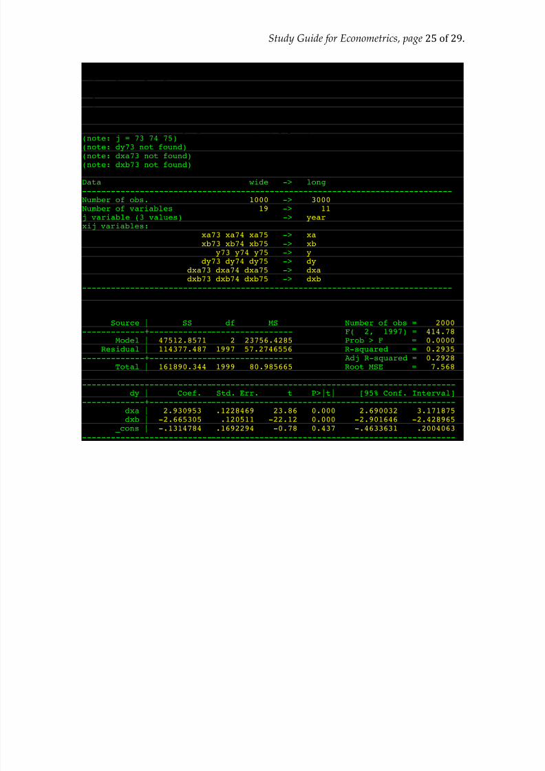
. gen dy74 = y74-y73
. gen dy75 = y75-y74
. gen dxa74 = xa74-xa73
. gen dxa75 = xa75-xa74
. gen dxb74 = xb74-xb73
. gen dxb75 = xb75-xa74
. reshape long xa xb y dy dxa dxb, i(id) j(year)(note: j = 73 74 75)(note: dy73 not found)(note: dxa73 not found)(note: dxb73 not found)
Data wide -> long-----------------------------------------------------------------------------Number of obs. 1000 -> 3000 Number of variables 19 -> 11 j variable (3 values) -> year xij variables:
xa73 xa74 xa75 -> xa xb73 xb74 xb75 -> xb
y73 y74 y75 -> y dy73 dy74 dy75 -> dy
dxa73 dxa74 dxa75 -> dxa dxb73 dxb74 dxb75 -> dxb
-----------------------------------------------------------------------------
. reg dy dxa dxb
Source | SS df MS Number of obs = 2000-------------+------------------------------ F( 2, 1997) = 414.78
Model | 47512.8571 2 23756.4285 Prob > F = 0.0000Residual | 114377.487 1997 57.2746556 R-squared = 0.2935
-------------+------------------------------ Adj R-squared = 0.2928Total | 161890.344 1999 80.985665 Root MSE = 7.568
------------------------------------------------------------------------------dy | Coef. Std. Err. t P>|t| [95% Conf. Interval]
-------------+----------------------------------------------------------------dxa | 2.930953 .1228469 23.86 0.000 2.690032 3.171875dxb | -2.665305 .120511 -22.12 0.000 -2.901646 -2.428965
_cons | -.1314784 .1692294 -0.78 0.437 -.4633631 .2004063------------------------------------------------------------------------------
8/3/2019 Metrics Guide 1
http://slidepdf.com/reader/full/metrics-guide-1 26/29
Study Guide for Econometrics, page 26of29.
Unit 8: Discrete and Limited Dependent Variables
Maximum-likelihood estimation
Philosophy: find the parameters that make the observation most likely.
General technique
1. Select a probability distribution to model the phenomenon.
2. Write out the likelihood of observing the outcome, as a functionof unknown parameters.
3. Find the values of the parameters that make the observation mostprobable.
Examples
Binomial outcome
Linear model with normally distributed unobservables
Binary outcome models: yi = 0 or yi = 1 .Objects of interest: what we want to know.
Predicted probabilities: P[ yi= 1 x
i]
Marginal effects: ∂P[ yi= 1 x
i] ∂x
i.
Linear probability model: OLS with binary outcome yi.
Advantages
Simplicity: easily calculated.
Ease of interpretation: ˆβ are estimated marginal effects; xi
ˆβ is predicted probability.
Permits IV and panel data techniques.
Disadvantages
Heteroskedasticity: given xi , e
itakes one of two values.
Implausible predicted probabilities: P[ yi =
1 xi] can be less
than 0 or greater than 1.
Inconsistency with models.
Maximum likelihood models
“Latent value”
Likelihood function: P[ yixi] = [1−CDF(−x
iβ )] yi [CDF(−x
iβ )](1− yi )
Choice of distribution for ei
Probit model: for normal distribution.
8/3/2019 Metrics Guide 1
http://slidepdf.com/reader/full/metrics-guide-1 27/29
Study Guide for Econometrics, page 27of29.
Marginal effects
Logit
Odds ratios
Interpretation of estimated coefficients
Not marginal effectsSign and relative magnitude only
Marginal effects at average, ∂P[ y = 1 x] ∂x (probit)
Odds ratio: P[ y = 1 x + 1] P[ y = 1 x] (logit)
Instrumental variables: the “forbidden regression”
(IV probit)
Logistic regression
Multiple discrete outcomesMultiple unordered outcomes: multinomial logit
Interpretation
Multiple ordered/ranked outcomes, no scale: ordered probit
Count data: Poisson regression
Censored regression
Tobit
Sample selection
Heckman
8/3/2019 Metrics Guide 1
http://slidepdf.com/reader/full/metrics-guide-1 28/29
Study Guide for Econometrics, page 28of29.
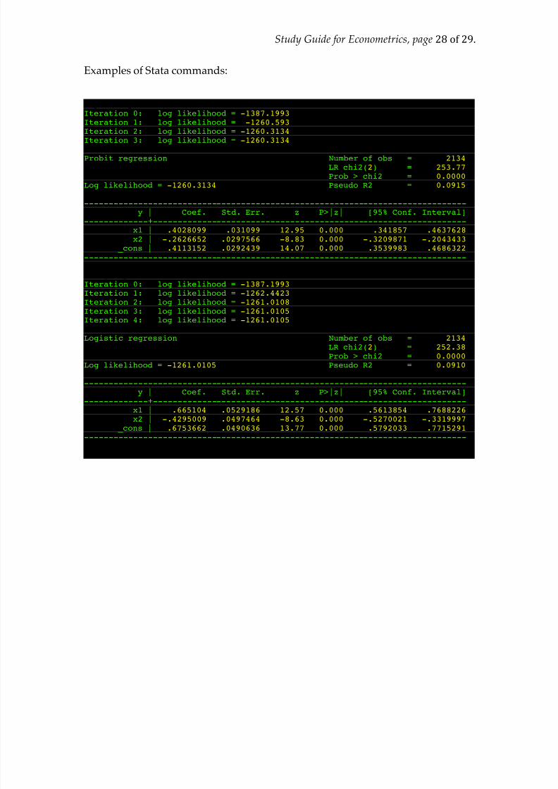
Examples of Stata commands:
. probit y x1 x2Iteration 0: log likelihood = -1387.1993Iteration 1: log likelihood = -1260.593Iteration 2: log likelihood = -1260.3134
Iteration 3: log likelihood = -1260.3134
Probit regression Number of obs = 2134LR chi2(2) = 253.77Prob > chi2 = 0.0000
Log likelihood = -1260.3134 Pseudo R2 = 0.0915
------------------------------------------------------------------------------y | Coef. Std. Err. z P>|z| [95% Conf. Interval]
-------------+----------------------------------------------------------------x1 | .4028099 .031099 12.95 0.000 .341857 .4637628x2 | -.2626652 .0297566 -8.83 0.000 -.3209871 -.2043433
_cons | .4113152 .0292439 14.07 0.000 .3539983 .4686322------------------------------------------------------------------------------
. logit y x1 x2Iteration 0: log likelihood = -1387.1993Iteration 1: log likelihood = -1262.4423Iteration 2: log likelihood = -1261.0108Iteration 3: log likelihood = -1261.0105Iteration 4: log likelihood = -1261.0105
Logistic regression Number of obs = 2134LR chi2(2) = 252.38Prob > chi2 = 0.0000
Log likelihood = -1261.0105 Pseudo R2 = 0.0910
------------------------------------------------------------------------------y | Coef. Std. Err. z P>|z| [95% Conf. Interval]
-------------+----------------------------------------------------------------x1 | .665104 .0529186 12.57 0.000 .5613854 .7688226x2 | -.4295009 .0497464 -8.63 0.000 -.5270021 -.3319997
_cons | .6753662 .0490636 13.77 0.000 .5792033 .7715291------------------------------------------------------------------------------

8/3/2019 Metrics Guide 1
http://slidepdf.com/reader/full/metrics-guide-1 29/29
Study Guide for Econometrics, page 29of29.
. mlogit y x1 x2 x3Iteration 0: log likelihood = -3433.7503Iteration 1: log likelihood = -3295.8062Iteration 2: log likelihood = -3289.9601Iteration 3: log likelihood = -3289.9381Iteration 4: log likelihood = -3289.9381
Multinomial logistic regression Number of obs = 3313LR chi2(6) = 287.62Prob > chi2 = 0.0000
Log likelihood = -3289.9381 Pseudo R2 = 0.0419
------------------------------------------------------------------------------y | Coef. Std. Err. z P>|z| [95% Conf. Interval]
-------------+----------------------------------------------------------------1 |
x1 | -.222846 .0407254 -5.47 0.000 -.3026663 -.1430256 x2 | .0026875 .0395999 0.07 0.946 -.074927 .080302 x3 | -.032302 .0392481 -0.82 0.410 -.1092268 .0446228
_cons | -.1885108 .0391199 -4.82 0.000 -.2651843 -.1118373 -------------+----------------------------------------------------------------2 |
x1 | -.7996707 .0541183 -14.78 0.000 -.9057406 -.6936007
x2 | -.1135117 .0509981 -2.23 0.026 -.2134661 -.0135573x3 | -.3267343 .051504 -6.34 0.000 -.4276803 -.2257884
_cons | -1.070102 .0547543 -19.54 0.000 -1.177419 -.9627856-------------+----------------------------------------------------------------3 | (base outcome)------------------------------------------------------------------------------