metrans project 07-12

On Sequencing of Container Deliveries to Over-the-Road Trucks from Yard Stacks

Final Report

METRANS PROJECT 07-12

July 23, 2008

Principal Investigator Shui Lam

Co-Investigator Burkhard Englert

Research Assistants Benson Tan Jeho Park

Shannon Foss

California State University, Long Beach Department of Computer Engineering and Computer Science

Long Beach, CA 90840 Tel: (562) 985-1552 Fax: (562) 985-7823 E-mail: [email protected]

i

mailto:[email protected]

DISCLAIMER

The contents of this report reflect the views of the authors, who are responsible for the facts and the accuracy of the information presented herein. This document is disseminated under the sponsorship of the Department of Transportation, University Transportation Centers Program, and California Department of Transportation in the interest of information exchange. The U.S. Government and California Department of Transportation assume no liability for the contents or use thereof. The contents do not necessarily reflect the official views or policies of the State of California or the Department of Transportation. This report does not constitute a standard, specification, or regulation.

ii

ABSTRACT

Containers unloaded from ships are typically kept on the terminal ground for a short duration until they are dispatched. Such containers are transported off the terminal ground either by train or by over-the-road trucks. This project focuses on the delivery of containers to over-the-road trucks. Through the use of a specifically developed simulation tool, we examine in this study the effect of container delivery methods on the mean truck turn time, as the container volume increases. Based on our simulation experiments we show that:

• Under continued growth the need for better sequencing of container delivery from yard stacks is inevitable.

• It is feasible to provide more intelligent and dynamic sequencing for the container delivery as an alternative to first-come-first-served, given the adoption of technology.

• Intelligent sequencing rules need not be complex. Simple heuristics such as Shortest Job First, Shortest Seek Time First or Elevator algorithm can be very effective in reducing truck turn time as well as queue size.

• Both Shortest Job First and Shortest Seek Time First have the drawback of starvation (some jobs may be continuously delayed by new arrivals). The Elevator algorithm has no such deficiency and exhibits comparable performance, thus should be preferable.

• Even with the most rudimentary system of one-day advance appointments, the terminal would be able to perform a sufficient amount of reshuffling to enable more efficient deliveries.

• Our simulation tool is sufficiently flexible to allow users to input parameters that reflect future condition of their terminal’s operations and determine if alternative sequencing rules for container delivery warrants implementation.

While the experiments carried out in this study are based on parameters that fit those at terminals in the Los Angeles/Long Beach Seaport, we believe that the methodology is applicable to a large number of container ports in the U.S. and abroad, and the simulation is designed to allow for flexible configuration.

iii

CONTENTS

DISCLAIMER . . . . . . . . . . . . . . . . . . . . . . . . . . . . . . . . . . . . . . . . ii

ABSTRACT . . . . . . . . . . . . . . . . . . . . . . . . . . . . . . . . . . . . . . . . . iii

DISCLOSURE . . . . . . . . . . . . . . . . . . . . . . . . . . . . . . . . . . . . . . . . v

LIST OF FIGURES . . . . . . . . . . . . . . . . . . . . . . . . . . . . . . . . . . . . . . vi

LIST OF TABLES . . . . . . . . . . . . . . . . . . . . . . . . . . . . . . . . . . . . . . . vi

INTRODUCTION . . . . . . . . . . . . . . . . . . . . . . . . . . . . . . . . . . . . . . . 1

BACKGROUND AND MOTIVATION . . . . . . . . . . . . . . . . . . . . . . . . . . . 1

ARRIVALS AND DELIVERIES OF IMPORT CONTAINERS. . . . . . . . . . . . . . . 3

CURRENT STATE OF OPERATION FOR CONTAINER DELIVERY AT THE LA/LB SEAPORT . . . . . . . . . . . . . . . . . . . . . . . . . . . . . . . . . . . . . . . 4

MODELING THE CONTAINER DELIVERY FROM THE IMPORT YARD STACKS . . 5

EXPERIMENTS . . . . . . . . . . . . . . . . . . . . . . . . . . . . . . . . . . . . . . . . 8

Assumptions . . . . . . . . . . . . . . . . . . . . . . . . . . . . . . . . . . . . . . . . 8 Arrival Distributions . . . . . . . . . . . . . . . . . . . . . . . . . . . . . . . . . . . . 10 Scheduling Algorithms . . . . . . . . . . . . . . . . . . . . . . . . . . . . . . . . . . 12 Simulation Design and Performance Measures . . . . . . . . . . . . . . . . . . . . . . 13 Simulation Implementation . . . . . . . . . . . . . . . . . . . . . . . . . . . . . . . . 15

SIMULATION RESULTS . . . . . . . . . . . . . . . . . . . . . . . . . . . . . . . . . . 16

Truck Turn Times . . . . . . . . . . . . . . . . . . . . . . . . . . . . . . . . . . . . 16 Components of Turn Time . . . . . . . . . . . . . . . . . . . . . . . . . . . . . . . . 19 Queue Sizes . . . . . . . . . . . . . . . . . . . . . . . . . . . . . . . . . . . . . . . . 22

COMPARISON AMONG SJF, ELEVATOR+, AND SSTF+ . . . . . . . . . . . . . . . . 23

EFFECTS OF APPOINTMENTS ON CONTAINER DELIVERY . . . . . . . . . . . . . 26

CONCLUSIONS . . . . . . . . . . . . . . . . . . . . . . . . . . . . . . . . . . . . . . . 28

REFERENCES . . . . . . . . . . . . . . . . . . . . . . . . . . . . . . . . . . . . . . . . 29

iv

DISCLOSURE

Project was funded in entirety under this contract to California Department of Transportation.

v

LIST OF FIGURES

Figure 1. Graphical User Interface for Simulation Program Run . . . . . . . . . . . . . . 7 Figure 2. An aerial view of container storage block of size 10x6, being serviced by one

transtainer. . . . . . . . . . . . . . . . . . . . . . . . . . . . . . . . . . . . . 8 Figure 3. Cross-sectional view of a container storage block, with stack heights of 3-4-5-5-4-3

across one bay of 6 stacks. . . . . . . . . . . . . . . . . . . . . . . . . . . . . 9 Figure 4. Interarrival Times Data Fitted with a Lognormal Distribution Function . . . . . 11 Figure 5. Pseudocode of the Simulation Program . . . . . . . . . . . . . . . . . . . . . . 16 Figure 6. Cumulative Distribution Function of Truck Turn Time, SJF vs. Elevator+ 24 . . . . Figure 7. Upper 20% of the Cumulative Distribution Function shown in Figure 5 25 . . . . .

LIST OF TABLES

Table 1: Container Volume at the Ports of Los Angeles and Long Beach . . . . . . . . . 2 Table 2: Number of lifts needed relative to position on stack . . . . . . . . . . . . . . . 10 Table 3: Best-fit Distributions for Interarrivals . . . . . . . . . . . . . . . . . . . . . . 10 Table 4: Sample Interarrival Time Statistics from Terminal X . . . . . . . . . . . . . . 11 Table 5: Truck Turn Times for Block Size 10x6, Exponential Arrivals . . . . . . . . . . 16 Table 6: Truck Turn Times for Block Size 10x6, Lognormal 1 Arrivals (i.e., Stdev=Mean) 17 Table 7: Truck Turn Times for Block Size 10x6, Lognormal 2 Arrivals (i.e.,Stdev=2*Mean) 17 Table 8: Mean Turn Times at Low Arrival Rate (One per 12 Minutes) for All Three Arrival

Distributions. . . . . . . . . . . . . . . . . . . . . . . . . . . . . . . . . . . . 17 Table 9: Mean Turn Times at Higher Arrival Rate (One per 4 Minutes) for All Three Arrival

Distributions. . . . . . . . . . . . . . . . . . . . . . . . . . . . . . . . . . . . 18 Table 10: Truck Turn Times for Block Size 10x6, Lognormal 2 Arrivals. Contrast between

Change in Arrival Rate and Change in Turn Time . . . . . . . . . . . . . . . 18 Table 11: Equipment Utilization Near Point of Instability . . . . . . . . . . . . . . . . 19 Table 12. Increase of Truck Turn Time as Block Size Increases, with Lognormal 2 Arrivals 19 Table 13: Mean Seek Time for Two Block Sizes with Lognormal 2 Arrivals . . . . . . . 20 Table 14. Mean Lift Time for Two Block Sizes with Lognormal 2 Arrivals 20 . . . . . . . . Table 15. Effect of Block Size on Equipment Utilization and Turn Time . . . . . . . . . 22 Table 16. Mean Queue Sizes for Block Size 10x6 . . . . . . . . . . . . . . . . . . . . . 22 Table 17. Mean Queue Sizes at Low Arrival Rate (One per 12 Minutes) for all Three Arrival

Distributions. . . . . . . . . . . . . . . . . . . . . . . . . . . . . . . . . . . 23 Table 18. Mean Queue Sizes at Higher Arrival Rate (One per 4 Minutes) for all Three Arrival

Distributions. . . . . . . . . . . . . . . . . . . . . . . . . . . . . . . . . . . 23 Table 19: Comparison of SJF and Elevator Turn Time Distributions . . . . . . . . . . . 26 Table 20: Gains from Reshuffling and Comparison between Two Reshuffling Schemes 27 . .

vi

INTRODUCTION

Containers unloaded from ships are typically kept on the terminal ground for a short duration until they are dispatched. Such containers are transported off the terminal ground either by train or by over-the-road trucks. This project focuses on the delivery of containers to over-the-road trucks. We examine in this study the effect of container delivery methods on the mean truck turn time, as the container volume increases. We provide:

1. Performance comparison of various container delivery methods for terminals with operating characteristics that can be customized to those in the LA/LB Twin Ports.

2. An understanding of the conditions under which alternative scheduling methods for container deliveries become advantageous.

3. A tool that can potentially be adopted by each terminal for short and long term planning in regards to policy of container delivery.

While the experiments carried out in this study are based on parameters that fit those terminals in the Los Angeles/Long Beach Seaport, we believe the methodology is applicable to a large number of container ports in the U.S. and abroad, and the simulation is designed to allow for flexible configuration. The concepts developed and the findings obtained in this project may easily be adopted in a simulation test bed developed in the METRANS project 05-11 by Ioannou and Chassiakos [5].

BACKGROUND AND MOTIVATION

Terminals in the Los Angeles/Long Beach Seaport are fortunate in that they typically occupy relatively large acreage of land. As a result, many of them had for a long time been able to deliver all containers on wheel to over-the-road trucks and hence no gantry equipment was needed for such deliveries. However, this is no longer true due to the rapid growth of cargo volume over the last decade and the fact that port space is limited. The cargo volume changes as shown in Table 1 [16, 17] depict a compound annual growth of 9.4% over the past decade. Moreover, from the same sources we found that since 1998 the inbound cargo volume has been about twice as much as the outbound volume. The effect of these trends on the way that containers are to be delivered is significant and to be expected. For example, at the APM Terminal of the Los Angles Port, containers bound for over-the-road trucks were 90% wheeled in 2005, and only 70% a year and a half later [1]. To deliver containers that are not on wheels require yard cranes and operators, the availability of which involves detailed scheduling. The problem’s urgency can only gain momentum as the trends of rapid growth of container traffic at the Twin Ports continue.

1

Table 1. Container Volume at the Ports of Los Angeles and Long Beach Numbers shown are in Millions of TEUs

Year POLA POLB Total Change from previous year % Change

1997 2.9 3.5 6.4 1998 3.4 4.1 7.5 1.1 17% 1999 3.8 4.4 8.2 0.7 9% 2000 4.9 4.6 9.5 1.3 16% 2001 5.2 4.5 9.7 0.2 2% 2002 6.1 4.5 10.6 0.9 9% 2003 7.1 4.7 11.8 1.2 11% 2004 7.3 5.8 13.1 1.3 11% 2005 7.5 6.7 14.2 1.1 8% 2006 8.5 7.3 15.8 1.6 11% 2007 8.4 7.3 15.7 ‐0.1 ‐1%

The scheduling of container delivery to over-the-road trucks is studied by Kim et al. [4]. They construct a dynamic programming model of the problem for a static case which assumes that all truck arrivals are known in advance. For the nondeterministic case where truck interarrival times are assumed to be exponential with a mean of 6 or 12 minutes, they compare a number of heuristic sequencing rules along with a reinforcement-learning-based method that they propose. Their comparison is in terms of delay beyond a specific due time after the arrival of the trucks. Under their assumed experimental parameters, their simulation results suggest the superiority of the reinforcement-learning-based method when the container pickup locations are more concentrated in a small number of yard-bays (as opposed to uniformly distributed). For target containers that are uniformly distributed throughout the stack storage area, they compared several heuristic sequencing rules: first-come-first-served (FCFS), uni-directional travel (UT), nearest-truck-first- served (NT), and the shortest processing time rule (SPT) and concluded that SPT performs best based on the minimization of delay cost. Lai and Leung [9] show in their simulation study that NT outperforms UT. Ng and Mak [13] consider a related but different sequencing problem of servicing a given number of empty trucks dispatched to transfer stacked containers from the export yard to a container vessel in a tightly spaced working lane. A deterministic case is formulated into an optimization problem of finding a sequence for the dispatched trucks to enter the working lane to receive the containers, with the objective of minimizing the total time required to serve all the dispatched trucks.

Jin, Liu and Gao [7] present an intelligent simulation method for regulation of container yard operations in a container terminal. Their method provides the functions of system status evaluation, operation rule and stack height regulation, and operation scheduling. In order to realize optimal operation regulation, they establish a control architecture based on a fuzzy artificial neural network. The regulation process includes two phases: a prediction phase which forecasts the future container quantity; an inference phase that makes decisions about the operation rules and the stack

2

height. The operation scheduling is a fuzzy multi-objective programming problem with operation criteria such as minimum ship waiting time and operation time. Their algorithm combines genetic algorithms with a simulation. Other comparable terminal truck delivery studies can be found in [11, 12, 15, 19].

The study by Kim et al. [4] in particular, however, makes four important assumptions, namely that (1) the truck interarrival time distribution are exponential, (2) the yard block configuration is fixed, and (3) the transfer time of container from a stack to the receiving truck is fixed, and (4) the speed of the yard crane movement is also fixed. Moreover only two truck pickup arrival rates are tested. For assumption (1), there is evidence that interarrival times distribution for container pickups may not be exponential, but could be lognormal or other distributions [8]. As with all operations involving human operators, processing times are never static. Machine movements that involve start and stop are often subject to acceleration and deceleration. Hence assumptions (3) and (4) should be relaxed and can be relaxed readily. As for the fixed yard block configuration assumption, we believe that the effectiveness of alternative scheduling strategies over FCFS may depend on the yard block configuration. It is therefore important to study the efficiency of container delivery sequencing rules based on alternative truck arrival distributions, varying arrival rates that reflect cargo volume changes, more realistic depiction of container transfer times and crane movements. We also believe it is important to examine the issue under the pressing problem of container volume growth as well as the industry trend toward adopting an appointment system for container pickups. In light of the fact that inbound cargo volume is twice that of outbound, performance improvement of the delivery of import containers can be expected to have a significant impact on the overall turn time performance for marine terminals.

ARRIVALS AND DELIVERIES OF IMPORT CONTAINERS

When a ship arrives at a marine terminal, containers on board will be unloaded according to a plan that has already been sent to the terminal ahead of time. Special priority containers that need to be unloaded first are noted. Each container to be unloaded is retrieved from the ship using a quay crane, placed onto the chassis being pulled by a utility terminal truck to be hauled to a predetermined yard area.

All containers unloaded to the terminal yard must be moved away, either by train or by truck. Those bound for distant locations (e.g., Chicago, Atlanta, etc.) are typically loaded onto trains using either on dock or near dock rail facilities. Those bound for local warehouses and short-haul destinations will be prepared for truck pickups. In this case, the container may be kept on wheels (e.g., for high-priority containers to be picked up shortly), or decked (placed in a stack). For a container to be on wheels the utility terminal truck driver will park the chassis and container in the specified wheeled area and its exact location will be input into the terminal’s computer. If the container is to be put in a stack then an equipment (e.g., a toploader, a straddle carrier) and one or more clerks will be there to remove the container from the chassis and place it in the stack. The clerk or the equipment records where in the stack the container was placed and inputs it into the computer. The utility terminal truck driver then returns back to the quay crane to pick up another container. This process is repeated until all containers that need to be unloaded are removed and placed into the yard. Empty containers are placed separately in their own area in the yard.

3

For containers to be delivered by trucks, the customers will be notified of their arrival. The customer is responsible for any arrangement necessary for their pickups. All import containers unloaded from a ship are expected to be removed, by train or by truck, from the terminal within a few days. Charge for storage will be levied for containers that remain in the terminal beyond a free storage period (four to seven days typical in the terminals at the LA/LB ports).

CURRENT STATE OF OPERATION FOR CONTAINER DELIVERY AT THE LA/LB SEAPORT TERMINALS

A shipper notified of their containers’ arrival will send their contracted truckers to pick them up at the terminal. For import container pickups, some terminals in the LA/LB seaports employ an hourly appointment system (e.g. Evergreen Terminal) while others do not (e.g., California United Terminal). Among those that have implemented an appointment system, some mandate its use (e.g., West Basin Container Terminal) while others keep it optional (e.g., TransPacific Terminal). For those that do not employ a pickup appointment system, information about a specific container pickup would be known only as the truck enters the terminal gate. As the trucker enters the terminal gate, he is issued a ticket printed with the container’s location where he proceeds to receive the container. The needed container may be on wheels or stacked. If the container is on wheels then the driver hooks up his truck to the chassis and pulls away. If the container is decked, something needs to be done on the part of the terminal while the driver waits for his container to be pulled from the stack pile and loaded onto his chassis. Such an operation requires an equipment, typically a yard crane or a transtainer, and an equipment operator. At the time the driver is issued a ticket for his transaction, a work instruction is generated to instruct the yard crane operator to proceed to the same location and make the delivery. With this mode of operation, a terminal can only assume that all or most of the import containers ready for delivery will be picked up within the free container storage time window (four to seven days are typical in the LA/LB ports). Which of those containers should be wheeled could at worst be a random selection or at best be the result of an educated guess based on previous trucker pickup behavior from historical data.

Terminals that employ an appointment system have the benefit of advance information of container pickup date and time, which may not be accurate due to factors such as missed appointment, traffic unpredictability, contingency appointments that can be cancelled without penalty, as reported in [3]. Due to this less precise nature of such an appointment system, wheel dwell time will tend to be longer than necessary, and the need for wheels higher. In any case, there is still a good chance that not all containers can be wheeled for delivery, especially as the container volume continues to grow and the terminal space is limited. Therefore, some container deliveries will still be made from stack and scheduling of transtainer and operator for their deliveries will still be required. To date these deliveries are being serviced largely on a first-come-first-served basis [2], though a few may have employed other heuristic, including the unidirectional travel algorithm [22]. The adoption of new technologies in terminal operations (e.g., RFIDs on trucks, dGPS antennas on gantry equipment that communicate with the terminal’s computer system to provide accurate inventory and positions of containers on the yard, etc.) makes the implementation of dynamic scheduling decisions feasible.

Whether or not an appointment system is used, the need for an efficient scheduling algorithm for the delivery of containers from the yard stack is clear, and the urgency of this need could only

4

increase over time due to the rapid growth of container volume at the LA/LB seaports. In this project we conduct a systematic evaluation of a suite of container delivery strategies that will enable a terminal to respond to the issue as the container volume grows.

MODELING THE CONTAINER DELIVERY FROM THE IMPORT YARD STACKS

We depict the container delivery problem with the following elements:

• The import yard consists of multiple yard blocks that may be grouped in one or more physically separate areas. Each block is made up with a number of bays of stacks of containers of a certain height. Hence the location of a container can be uniquely represented by four numbers: the block number, the bay number within a block, the stack number within a bay, and the height that indicates where in a stack the container is stored.

• Each area of yard blocks is serviced by a given set of equipment such as transtainers.

• A queue of trucks is maintained for each yard block for those trucks waiting for containers from that block.

• Trucks enter the terminal at random times, each for a specific container from some yard block. Each truck will join the queue for the yard block where the container it is to pick up is located. The trucks will be serviced, first-come-first-served or using other sequencing rules that will be described later in the Experiments Section.

A simulation program was developed using the C# programming language to implement this model. The simulation program is started when a user invokes it through the graphical user interface shown in Figure 1. The form on the graphical user interface is designed to allow a user to define:

� The grounded container storage area configuration in terms of the number of areas, the number of blocks in each area, the dimension of the block giving the number of bays, number of stacks per bay and the maximum height of each stack.

� Resources allocated to servicing each area in terms of the number of equipment.

� Equipment type and equipment operating parameters. The current form provides only one choice, namely RTG (rubber tired gantry) or transtainer. Other equipment types and their operating parameters can be added as needed. Equipment operating parameters for transtainers include trolley speed, trolley movement time for one container length (to account for startup and stop time involved in trolley movements), time to move gantry from the current position to the stack where the needed container is located, and the time for lifting one container. The timing elements to be input are based on observed measurements or projected operating characteristics that consist of minimum, maximum and mean values. These values will be used as parameters in triangular distributions for the generation of trolley startup time, gantry movement time as well as lift time for the handling of each container in the simulation.

5

� Cargo pickup volume and characteristics in terms of arrival pattern and arrival rate. Two different arrival distributions are included in the current simulation: exponentially distributed interarrival times, and lognormally distributed interarrival times. For the lognormal distribution user can also specify the amount of standard deviation as a factor of the mean. The rationale for this selection of arrival patterns will be explained in the next section. Volume of the pickup load is depicted by the mean interarrival time, which user can input in the form.

� Instead of TEU-based by default, user can indicate the dominant container size being handled in the terminal’s container storage area.

� The duration of a simulation and the number of iterations the user wishes to run in the experiment.

� The type of output for the simulation results. User may choose averages only (showing statistics collected during the simulation experiment), raw data (giving all performance measures collected for each transaction), or both.

The graphical user interface also shows progress of the simulation run, as well as provides prompts to the user about what to do next, in a window on the right side of the display as depicted in Figure 1.

6

Figure 1. Graphical U

ser Interface for Simulation Program

Run

7

EXPERIMENTS

Assumptions

While the simulation program we developed allows for a comprehensive simulation of the container delivery in a terminal with an import yard of any size in a flexibly defined configuration, a closer look at the model led us to recognize that two levels of decision are involved in container delivery : resource allocation in terms of the number of equipment to be assigned to each area with one or more blocks, and scheduling of the truck in a queue to service next; the latter being the main object of investigation in this project. In order to avoid a clouding of the comparison results, we have conducted the simulation experiments with a simplified yard configuration. Specifically, we consider the scenario of a single block of container stacks configured into a rectangular shape consisting of 10 or more bays each of 6 stacks of a maximum height of 5 containers, and one transtainer is allocated for moving containers from the stacks onto trucks that come for the pickup. The objective of the experiments is to compare several scheduling algorithms and their performance at the various loads in terms of arrival rates. The block size varies from 10 to 60 bays, all with 6 stacks each. The increased block size represents the increased span of container storage area a transtainer is designated to service as a result of increased use of grounded delivery. For a given truck arrival rate, the comparison of performance between different block sizes allows us to see the effect of travel distance of the transtainer under different scheduling rules. The maximum height of a container stack within a block is 5 containers. Due to safety consideration, containers are typically stacked with reduced heights toward the edge of the block. Figure 2 shows a top view of a block of size 10x6, with a transtainer servicing the block. Figure 3 shows a cross-sectional view of a block of stacks with heights 3-4-5-5-4-3 of the 6 stacks across one bay.

6 Stacks

10 Bays

Transtainer

Figure 2. An aerial view of container storage block of size 10x6, being serviced by one transtainer.

8

Figure 3. Cross-sectional view of a container storage block, with stack heights of 3-4-5-5-4-3 across one bay of 6 stacks..

For the equipment speed, three components need to be considered: trolley speed measures how fast the transtainer moves up and down the block from one bay of stacks to another, gantry speed measure how fast the gantry can move across a bay from one stack to another, and lift speed measures the time it takes to lift a container from one position and lay it down on another position. For the lift speed we assume a range from 28 seconds to 1 minute 41 seconds, with an average of 49.4 seconds. For the gantry movement across a container bay we assume a range from 19 seconds to 53 seconds, with an average of 27.7 seconds. Both of these lift times and gantry movement times are based on an actual measurement of transtainer operations in a marine terminal at the LA/LB ports by James and Rodriguez [6]. The trolley movement consists of two components: a startup component and a uniform component after startup. The startup component is assumed to range from 19 seconds to 39 seconds, with an average of 28.5 seconds, based also on measurements obtained by James and Rodriguez. This startup component accounts for the time it takes the trolley to start as well as stop the movement. These measurements provide the parameters of triangular distributions for the generations of times we need in our simulation. The uniform component provides the timing of the trolley movement after the startup, and is calculated using half of the 264 feet/minute full speed specification of a Mitsubishi model of rubber tired gantry crane [10]. The trolley and gantry movements contribute to the time required to reach the next stack where the needed container is to be retrieved. This time is referred to as the seek time.

Our simulation further takes into account all “auxiliary lifts” that are necessary for container shuffling in order to reach a container deep in a stack, and the possible reshuffling of some or all of those removed containers. Reshuffling will not be necessary when space is available on a nearby stack in the same bay. Namely if the requested container is at the top of a stack one lift is necessary. If the requested container is the second container from the top and no space is available on a nearby stack to leave the top container on a permanent basis, three lifts are necessary, the first to move the top container to the side, the second to load the requested container, and finally the third to move the top container back onto the top of its original stack. However, only two lifts would be needed if space is available to leave the top container there permanently. Based on this reasoning the number of lifts can be easily determined based on the position of the container needed for delivery as shown in Table 2. With the help of dGPS antennas on gantry equipment the new locations of all relocated containers can be communicated to and recorded in the terminal’s computer instantaneously

9

Table 2: Number of lifts needed relative to position on stack

Position of a container on stack

Number of lifts needed to load container without reshuffling

Number of lifts needed to load container with reshuffling

First 1 1 Second 2 3 Third 3 5 Fourth 4 7 Fifth 5 9

Arrival Distributions

For the simulation, arrivals are generated randomly according to some selected distribution functions. Exponential distribution has long been the norm for such use [see for example 4, 14 and 18]. However, the monitoring truck arrivals at a marine terminal (referred to as Terminal X) at the Port of Los Angeles provide strong evidence that lognormal distribution may be a better fit for truck arrivals, as shown in Table 3 from Lam et al. [8]. The table shows the results of fitting the interarrival time data streams obtained for four monitoring sessions at Terminal X in four separate days in April and May of 2005 with four distributions: exponential, normal, lognormal, and gamma, and found lognormal to be the best fit in nine of the 12 cases. While other distribution functions may perform even better than lognormal, it is important to point out that exponential is not found to be the best fit in a single case. Figure 4 shows a sample arrival data collected in Lam’s study. The data in the figure is reported in terms of interarrival times that are fitted with a lognormal distribution function.

Table 3: Best-fit Distributions for Interarrivals

Best fit for interarrival data Lognormal Gamma

Day1 Bobtail Entry Day1 Main Entry Day1 Both Entries

Best fit Best fit Best fit


Best fit Best fit Best fit


Best fit Best fit

Best fit Day4 AM Bobtail Entry Day4 AM Main Entry Day4 AM Both Entries

Best fit Best fit

Best fit

10

Figure 4. Interarrival Times Data Fitted with a Lognormal Distribution Function

In light of this evidence, we have decided to use both the exponential and lognormal distributions for the generation of truck arrivals for container pickups in our simulation experiments. While the exponential distribution function is defined by a single parameter, the mean, the lognormal distribution function requires two parameters: mean and standard deviation. We have chosen two settings for the two parameters: (1) standard deviation = mean, and (2) standard deviation = twice the mean. The rationale for this choice stems from the data collected during the monitoring of truck arrivals at Terminal X as part of the study by Lam et al. [8]. As illustrated in Table 4, the standard deviation to mean ratios of the interarrival time data at the bobtail gate and the main gate during the four monitoring sessions on four separate days range from 0.85 to 1.50. We have therefore selected ratios of 1 and 2 for the lognormal parameters in our experiment to be compatible with these findings.

Table 4: Sample Interarrival Time Statistics from Terminal X

Monitoring Bobtail Main Gate Session Entry Entry

Mean Standard Deviation

Stdev / Mean Mean Standard

Deviation Stdev / Mean

Day 1 1.95 2.78 1.43 0.71 0.60 0.85

Day 2 2.26 3.40 1.50 0.58 0.50 0.86

Day 3 1.70 1.51 0.89 0.50 0.44 0.88

Day 4 1.54 1.45 0.94 0.69 0.73 1.06

11

For the arrival rate, we consider a base volume with an arrival rate of one truck every 12 minutes and then consider 10, 8, 6, 4 and 2 minutes mean intervals between arrivals to represent the increase of volume. For each of these arrival rates, we compute the corresponding mean interarrival time and run a simulation experiment of each of these three arrival distributions: exponential, lognormal with standard deviation=mean (refer to as lognormal 1 hereafter), and lognormal with standard deviation=2*mean (refer to as lognormal 2).

Scheduling Algorithms

We next describe the scheduling algorithms tested:

1. First-come-first-served (FCFS). In this case trucks are served in the order of their arrival time at the terminal. Currently this is the algorithm most commonly used in practice.

2. Shortest-Job-First (SJF). The equipment will proceed to serve the truck with the shortest transaction time, which is the sum of the time it takes the equipment to move to the bay and the stack where the requested container is in, plus the time for the equipment to access and transfer the container onto the truck. This is equivalent to the SPT rule described by Kim et al. in [4] and was found to be superior to other heuristics they tested.

3. The Elevator algorithm (Elevator). In this case the equipment services requests of containers much the same way an elevator is designed to service passenger requests from various floors. Specifically, the equipment travels only in one direction along the length of the block, servicing trucks requesting containers from the bays of stacks that it passes in order until no more request remain in the direction of travel. At that point, the equipment reverses its direction, again servicing trucks requesting containers from the bays it passes in that direction. If there are two or more containers to be delivered from the same bay, the same elevator concept is applied along the stacks in that bay. With this algorithm the equipment will always finish servicing all existing requests from the current bay position before moving to another bay. This algorithm is similar to UT described in [4].

4. The Elevator Plus algorithm (Elevator+). This algorithm uses the same logic as the Elevator algorithm, except among the multiple requests of containers from the same bay priority is given to the one that requires the least number of lifts.

5. Shortest-Seek-Time-First algorithm (SSTF). In this case the equipment always services the truck requesting a container from a bay closest to its current location. If there are two or more containers to be delivered from the same bay, the container closest to the current gantry position of the equipment will be retrieved first. The time to reach the stack location of the needed container from the equipment’s current spot is referred to as the seek time, hence this algorithm is called the shortest-seek-time-first algorithm. As with the Elevator algorithm, SSTF will always finish servicing all existing requests from the current bay position before moving to another bay. This algorithm is similar to NT described in [4].

6. Shortest-Seek-Time-First Plus algorithm (SSTF+). This algorithm uses the same logic as the SSTF algorithm, except among the multiple requests of containers from the same bay priority is given to the one that requires the least number of lifts.

7. Circular-Scan Plus algorithm (C-Scan+). This algorithm works the same way as the Elevator+ algorithm with the following exception: when the equipment reaches the end of the block it returns all the way to the beginning of the block and starts again servicing requests from there. When using the Elevator+ algorithm, it takes equipment a complete

12

__________

round trip to return to the same end of the container block but only half of a round trip to revisit the block’s middle section. Hence containers in the two ends of a block tend to suffer longer waits. C-Scan+ is designed to limit any bias that may exist against containers that are placed at the ends of a yard block.

The Elevator, SSTF, and C-Scan are named after algorithms developed for scheduling requests for access to hard disks in computer systems (see [21], for example, for their definitions in that context.) These algorithms are adopted and modified to fit the problem of container deliveries from yard stacks in a marine terminal setting. The Elevator and SSTF algorithms are referred to as UT and NT, respectively, in [4, 9]. We chose to use “Elevator” and “SSFT” because we believe these names capture vividly the way these algorithms work. Elevator+, SSTF+ and C-Scan+ are variations of these algorithms that are applicable to the problem of servicing container yard stacks.

Simulation Design and Performance Measures

Since the objective of this project is to investigate the potential benefits of using different sequencing rules for servicing truck pickups of containers, we design our simulation depicting only the container delivery aspect of terminal operations. Truck turn time, the span of time from a truck’s arrival at the terminal to its departure with the needed container, is the main measure of performance since it is the major component of truck turn times in normal terminal operations. In order to ensure that the performance reflects the effect of scheduling algorithms rather than other resource issues such as allocation of equipment, operators and space, we depict the yard as a single block of various lengths in terms of number of bays, and the width of the block is set at a constant of 6 stacks. The block size we experiment varies from 10x6 to 60x6 stacks. The increased block length reflects partly variations in block sizes observed in different terminals at the LA/LB ports and partly the projected need for increased number of grounded containers to be delivered as a result of increased volume. The stack heights are set at 5 maximum, with the height on both ends reduced for safety consideration, resulting in a cross-sectional configuration of 3-4-5-5-4-3 as explained earlier.

Other performance measures we collected include the following:

• Wait time: the time from a truck’s arrival at the terminal gate to the moment it gets to be serviced.

• Seek time: the time it takes the equipment to reach the stack where the needed container is located from its current location.

• Lift time: the total time for the equipment to lift the needed container and place it onto the truckbed, plus all the “auxiliary lifts” that may be necessary for reaching the needed containers and reshuffling the displaced containers.

• Turn time1: the span of time from a truck’s arrival at the terminal to its departure with the needed container, which is the sum of wait time, seek time and lift time.

• Queue size: the average size of the truck queue through the simulation duration. • Customers served: the number of trucks to which containers are delivered.

1 The turn time measured in our simulation does not explicitly include truck driving time from entry gate to yard stacks on arrival or from yard stacks to exit gate on departure. However this exclusion will not affect the comparison results since they are excluded from turn times for all algorithms.

13

The simulation is run for a duration of 24 hours or until all containers in the block are delivered, whichever occurs first, for each combination of the following parameters:

• Block size = 10x6, 15x6, 20x6, 30x6, 40x6, 45x6, 60x6 • Mean interarrival time = 12, 10, 8, 6, 4, 2 (all in minutes) • Scheduling algorithm = FCFS, SJF, Elevator, Elevator+, SSTF, SSTF+, C-Scan+ • Arrival distribution = exponential, lognormal 1, lognormal 2

Each run is iterated 100 times and statistics on the selected performance measures are collected. The iteration reflects a common operational practice in marine terminals where reshuffling of container stacks will take place each night to consolidate the remaining containers in the yard blocks, and make room for new shipments of containers the next day. If an appointment system is adopted so that the terminal will have information about pickup demands for the next day, the reshuffling can take advantage of this information and place the needed containers in a concentrated, hence smaller block, or place them on or near the top stack positions. Such a procedure may have the consequence of mitigating the benefit of scheduling algorithms that make use of the containers’ stack positions in selecting the next truck to service. To investigate such effects, a second set of experiments has been conducted with the following parameters, and the results are reported in the section on Effects of Appointments on Container Delivery.

• Block size = 10x6 with stack heights 3-4-5-5-4-3 vs. 20x6 with stack heights 1-2-3-3-2-1 vs. 20x6 with stack heights 2-2-2-2-2-2

15x6 with stack heights 3-4-5-5-4-3 vs. 30x6 with stack heights 1-2-3-3-2-1 vs. 30x6 with stack heights 2-2-2-2-2-2



• Mean interarrival time = 12, 10, 8, 6, 4, 2 (all in minutes) • Scheduling algorithm = FCFS, SJF, Elevator, Elevator+, SSTF, SSTF+, C-Scan+ • Arrival distribution = exponential, lognormal 1, lognormal 2

This experiment is designed to find out how much, if any, performance improvements can be expected through reshuffling, and which reshuffling scheme (short block, pyramid style reduced height stacks 1-2-3-3-2-1, or rectangle style reduced height stacks 2-2-2-2-2-2) yields greater performance gains. All three configurations of the reshuffled blocks hold the same number of containers. For example, a short block 10x6 of the original heights 3-4-5-5-4-3 holds 240 containers, and so do the two reduced heights blocks of 20x6 with 1-2-3-3-2-1 stacks and 20x6 with 2-2-2-2-2-2. Mean turn time for truck pickups from each of these blocks will be compared with that from a block of a “normal” size (e.g., 20x6 in this illustration) that consists of containers that may or may not be picked up on the same day.

It should be noted that some terminals in the LA/LB ports implement hourly appointments. In this case containers can be batched and organized according to the hours of their pickup so that the seek time and lift time will be the minimum of near minimum, The experiment described above is designed to investigate potential benefits of appointments, even when a rudimentary appointment- by-day system (as opposed to by hour) is used. This finding could be useful in convincing

14

skeptics of the usefulness of appointments based on the consideration that appointments are difficult to keep due to traffic unpredictability. More discussions on appointments for container pickups will be given in the Effects of Appointments on Container Delivery section.

Simulation Implementation

The simulation was implemented with an object-oriented program written using the C# programming language. In the program the container pickup and delivery operations are abstracted to two types of events: truck arrival and truck departure. Truck arrival events are generated randomly according to a selected arrival distribution with a given arrival rate, and departure events are generated when the truck is selected to receive the container so the time the truck can leave the terminal with the needed container can be correctly computed. The time it takes to complete the delivery is the sum of seek time and lift time, both randomly generated using triangular distributions based on range and average parameters of the delivery equipment speeds from user input. Parameters used for our simulation experiments are explained in detail earlier in the Assumptions Section. An event queue is maintained in event time order. The simulation is moved forward by removing the next event from the event queue, advancing the system clock to this event and performing appropriate action according to the event type until the event queue is empty.

A truck queue is maintained for each yard stack area to help implement the various delivery sequencing rules. Trucks that have arrived but not yet assigned an equipment for service are placed in the truck queue. When an equipment becomes available, it is assigned to the truck selected from the truck queue based on the sequencing rule in consideration. The definition of all sequencing rules tested in our experiments are explained in the Scheduling Algorithms Section.

The program execution begins with the input of simulation parameters through the graphical user interface. Simulation parameters needed include: container storage yard configuration, type and number of equipment, equipment operating parameters, truck pickup arrival distribution and arrival rate, how long to run the simulation, etc. The pseudocode below depicts the heart of the simulation logic. To make sure that the performance comparison is based on scheduling difference alone as opposed to the difference in arrivals for pickups, we use the same arrivals stream for all scheduling algorithms.

Do for each priority scheduling algorithm Repeat

Reset yard stacks, truck queue, container delivery equipment status and system clock; Clear event queue, remove first arrival in arrivals stream and insert it into event queue; While system clock < simulation duration and event queue not empty do

Get next event from event queue and advance system clock to time of this event; Collect relevant performance data since last event till now;

Case 1: Next event is a truck arrival event Remove next arrival from arrivals stream and insert it into event queue sorted based on time of event;

Look for an idle equipment; If none found, then

Add the truck to the end of the truck queue; Else

Start servicing this truck with the available equipment to make delivery; Generate a truck departure event and insert it into the event queue sorted in order of

15

event time; End if; Case 2:Next event is a truck departure event

Mark container picked up by this truck as taken; Rearrange containers in the stack to reflect the removal of the departing truck’s container; Collect relevant performance data related to the departing truck; If truck queue is empty, then

Set equipment assigned to the departing truck as idle; Else

Identify the truck to service next in the truck queue based on the scheduling algorithm; Generate a truck departure event for the chosen truck and insert it into the event

queue sorted in order of event time; End if; End while;

Until all iterations done; Compute means and standard deviations of all performance data collected from all iterations and output to file;

End do;

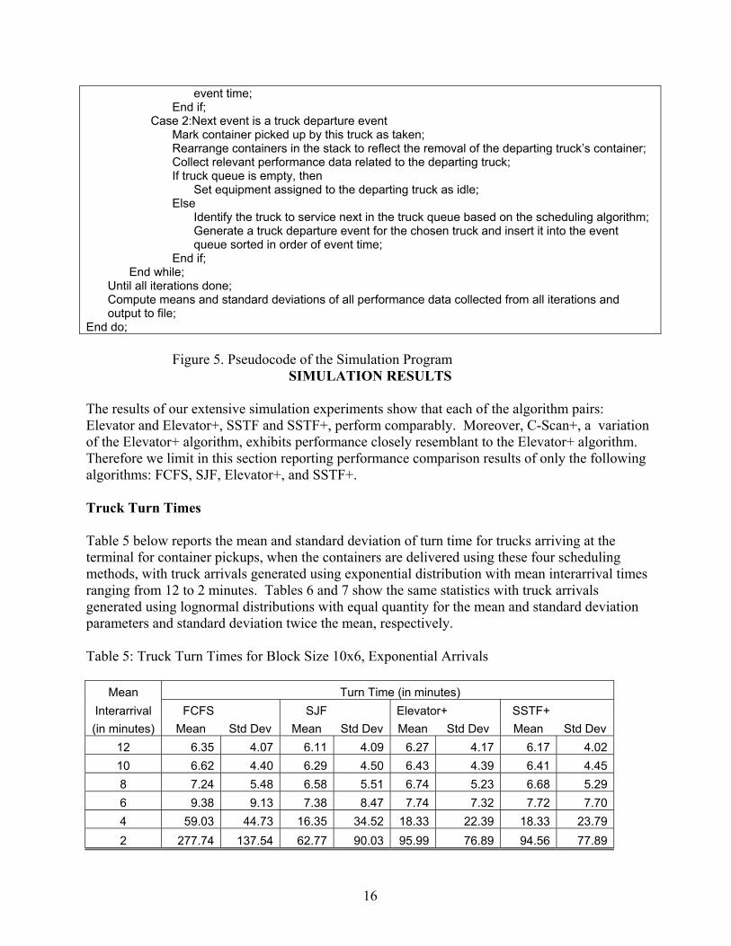
Figure 5. Pseudocode of the Simulation Program SIMULATION RESULTS

The results of our extensive simulation experiments show that each of the algorithm pairs: Elevator and Elevator+, SSTF and SSTF+, perform comparably. Moreover, C-Scan+, a variation of the Elevator+ algorithm, exhibits performance closely resemblant to the Elevator+ algorithm. Therefore we limit in this section reporting performance comparison results of only the following algorithms: FCFS, SJF, Elevator+, and SSTF+.

Truck Turn Times

Table 5 below reports the mean and standard deviation of turn time for trucks arriving at the terminal for container pickups, when the containers are delivered using these four scheduling methods, with truck arrivals generated using exponential distribution with mean interarrival times ranging from 12 to 2 minutes. Tables 6 and 7 show the same statistics with truck arrivals generated using lognormal distributions with equal quantity for the mean and standard deviation parameters and standard deviation twice the mean, respectively.

Table 5: Truck Turn Times for Block Size 10x6, Exponential Arrivals

Mean Interarrival (in minutes)

Turn Time (in minutes) FCFS

Mean Std Dev SJF

Mean Std Dev Elevator+ Mean Std Dev

SSTF+ Mean Std Dev

12 6.35 4.07 6.11 4.09 6.27 4.17 6.17 4.02 10 6.62 4.40 6.29 4.50 6.43 4.39 6.41 4.45 8 7.24 5.48 6.58 5.51 6.74 5.23 6.68 5.29 6 9.38 9.13 7.38 8.47 7.74 7.32 7.72 7.70 4 59.03 44.73 16.35 34.52 18.33 22.39 18.33 23.79 2 277.74 137.54 62.77 90.03 95.99 76.89 94.56 77.89

16

Table 6: Truck Turn Times for Block Size 10x6, Lognormal 1 Arrivals (i.e., Stdev=Mean)


Turn Time (in minutes) FCFS Mean Std Dev

SJF Mean Std Dev

Elevator+ Mean Std Dev

SSTF+ Mean Std Dev

12 5.44 3.08 5.37 3.09 5.39 3.11 5.40 3.11 10 5.69 3.44 5.56 3.48 5.6 3.50 5.60 3.54 8 6.38 4.46 5.94 4.73 6.05 4.29 6.04 4.40 6 8.50 8.11 6.91 8.36 7.13 6.87 7.07 7.26 4 53.40 41.73 15.82 34.53 17.53 22.04 17.48 23.34 2 280.48 138.53 63.12 91.41 96.05 77.95 95.62 78.73

Table 7: Truck Turn Times for Block Size 10x6, Lognormal 2 Arrivals (i.e.,Stdev=2*Mean)


Turn Time (in minutes) FCFS Mean Std Dev

SJF Mean Std Dev

Elevator+ Mean Std Dev

SSTF+ Mean Std Dev

12 7.71 5.50 7.06 5.76 7.33 5.55 7.36 5.72 10 8.84 6.81 7.66 7.12 8.00 6.46 8.00 6.72 8 10.97 9.35 8.61 9.31 9.20 8.22 9.17 8.56 6 18.27 19.30 10.81 16.45 12.02 13.14 11.89 13.86 4 73.31 60.20 21.05 42.11 25.39 31.36 25.92 33.87 2 286.01 141.76 65.78 89.72 98.92 80.18 100.00 83.29

Several observations from Tables 5-7 are worth noting:

1. With all three arrival patterns the mean turn times at the lowest arrival rate (one per 12 minutes) are comparable for all four scheduling methods, as illustrated in the comparison in Table 8.

Table 8. Mean Turn Times at Low Arrival Rate (One per 12 Minutes) for all Three Arrival Distributions. Turn Times are in Minutes.

Arrival Distribution

FCFS Mean Turn Time

SJF Mean Turn Time

Elevator+ Mean Turn Time

SSTF+ Mean Turn Time

Exponential 6.35 6.11 6.27 6.17

Lognormal 1 5.44 5.37 5.39 5.40 Lognormal 2 7.71 7.06 7.33 7.36

2. The advantage of the three alternative algorithms to FCFS becomes obvious as the arrival rate increases. In particular, when the arrivals are 4 minutes apart on average, the mean turn times with FCFS become much higher than 30 minutes with all three arrival distributions, rendering the performance unacceptable according to current industry standard in the Southern

17

California region. The other three algorithms, however, still produce a mean turn time below the 30-minute limit guideline. This comparison is depicted in Table 9.

Table 9. Mean Turn Times at Higher Arrival Rate (One per 4 Minutes) for all Three Arrival Distributions. Turn Times are in Minutes.


FCFS Mean Turn Time

SJF Mean Turn Time

Elevator+ Mean Turn Time

SSTF+ Mean Turn Time

Exponential 59.03 16.35 18.33 18.33

Lognormal 1 53.40 15.82 17.53 17.48 Lognormal 2 73.31 21.05 25.39 25.92

3. The turn times for lognormal 2 arrivals are consistently higher than their counterparts for exponential or lognormal 1 arrivals. These findings highlight the importance of proper modeling of the arrival process.

4. Mean turn time increases as the arrival rate increases, as expected, for all scheduling algorithms. The pace of change, however, appears to be slower with the three alternative algorithms compared with FCFS, as illustrated in Table 10. The drastic increases in turn times from the arrival rate of one in 6 minutes to one in 4 minutes, and from one in 4 minutes to one in 2 minutes reflect saturation, a situation when the demand for service has reached or is near the equipment capacity, as illustrated in Table 11. The system performance becomes unstable beyond this point,

Table 10: Truck Turn Times for Block Size 10x6, Lognormal 2 Arrivals Contrast between Change in Arrival Rate and Change in Turn Time


% Change In Arrival Rate

Turn Time (in minutes) FCFS Mean % Change

SJF Mean % Change

Elevator+ Mean % Change

SSTF+ Mean % Change

12 7.71 7.06 7.33 7.36 10 20.00% 8.84 14.66% 7.66 8.50% 8.00 9.14% 8.00 8.70% 8 25.00% 10.97 24.10% 8.61 12.40% 9.20 15.00% 9.17 14.63% 6 33.33% 18.27 66.55% 10.81 25.55% 12.02 30.65% 11.89 29.66% 4 50.00% 73.31 301.26% 21.05 94.73% 25.39 111.23% 25.92 118.00% 2 100.00% 286.01 290.14% 65.78 212.49% 98.92 289.60% 100.00 285.80%

18

Table 11: Equipment Utilization Near Point of Instability for Block Size 10x6



Equipment Utilization (%) FCFS SJF Elevator+ SSTF+

Exponential 6 64.43 63.34 62.59 62.48

4 94.78 87.63 86.06 86.08

2 99.73 99.56 99.58 99.57

Lognormal 1 6 65.40 64.55 63.70 63.69

4 94.13 87.43 85.54 85.62

2 99.73 99.54 99.57 99.57

Lognormal 2 6 66.33 63.27 61.90 61.97

4 91.10 82.54 80.71 80.98

2 99.62 99.02 99.16 99.12

5. The mean turn time increases as the block length increases. This is true for all three arrival distributions under all four sequencing rules. We will further analyze this phenomenon in the next section. Table 12 shows this trend for the case of lognormal 2 arrivals at a rate of one per 12 minutes.

Table 12. Increase of Truck Turn Time as Block Size Increases, with Lognormal 2 Arrivals

Block Size


Turn Time (in minutes) FCFS

Mean % Change SJF

Mean % Change Elevator+

Mean % Change SSTF+ Mean % Change

10x6 12 7.71 7.06 7.33 7.36 15x6 12 9.70 25.81% 8.56 21.25% 8.77 19.65% 8.70 18.21% 20x6 12 12.50 28.87% 10.32 20.56% 10.59 20.75% 10.46 20.23% 30x6 12 17.45 39.60% 12.72 23.26% 12.82 21.06% 12.55 19.98% 40x6 12 27.45 57.31% 16.14 26.89% 16.23 26.60% 15.94 27.01% 45x6 12 34.62 26.12% 17.89 10.84% 17.89 10.23% 17.61 10.48% 60x6 12 55.02 58.93% 21.67 21.13% 21.96 22.75% 21.26 20.73%

Components of Turn Time

The turn time represents the sum of seek time, lift time and wait time defined in the previous section. Tables 13 and 14 show the seek time and lift time statistics of the four scheduling algorithms for two block sizes with lognormal 2 arrivals.

19

Table 13: Mean Seek Time for Two Block Sizes with Lognormal 2 Arrivals


Block Size


Mean Seek Time (minutes) FCFS SJF Elevator+ SSTF+

Lognormal 2 10x6 12 1.35 1.32 1.29 1.29

10 1.35 1.33 1.27 1.26

8 1.34 1.29 1.21 1.22

6 1.35 1.25 1.14 1.14

4 1.35 1.15 0.95 0.96

2 1.35 0.83 0.64 0.64 30x6 12 3.30 2.95 2.84 2.81

10 3.32 2.80 2.64 2.61

8 3.31 2.55 2.32 2.29

6 3.32 2.15 1.79 1.79

4 3.31 1.57 1.06 1.06

2 3.33 0.92 0.65 0.66

Table 14. Mean Lift Time for Two Block Sizes with Lognormal 2 Arrivals


Block Size


Mean Lift Time (minutes) FCFS SJF Elevator+ SSTF+

Lognormal 2 10x6 12 3.18 3.16 3.17 3.19

10 3.04 3.02 3.03 3.03

8 2.87 2.82 2.84 2.84

6 2.57 2.49 2.52 2.52

4 2.51 2.22 2.34 2.35

2 2.49 1.37 1.71 1.71 30x6 12 3.49 3.47 3.49 3.47

10 3.44 3.41 3.44 3.41

8 3.42 3.36 3.39 3.39

6 3.41 3.22 3.32 3.32

4 3.40 2.67 3.06 3.05

2 3.38 1.40 1.93 1.93

Observations from Tables 13 and 14 presented below apply to all three forms of interarrival distribution tested: exponential, lognormal 1, and lognormal 2.

1. With FCFS, the mean seek time stays the same for a given block size, regardless of the arrival rate. This is expected since the selection decision for the next container to deliver is independent of the location of the container relative to the current location of the equipment. The mean seek time however does increase as the block size increases since the distance to travel lengthens with larger blocks.

20

2. With all other three algorithms the mean seek time decreases as arrival rate increases. Furthermore, the changes are much more prominent with the Elevator+ and SSTF+ algorithms since the seek time is the dominant decision variable in choosing the next container to service in these algorithms and there are more choices for containers to pick for delivery next at higher arrival rates.

3. The mean lift time for all three alternative algorithms to FCFS decreases as arrival rate increases, since all three uses lift time in their selection decision for the next container to deliver. The higher the arrival rate, the more containers there are to choose from to deliver next. Incorporating lift time in the delivery sequencing should therefore lead to reduced mean lift time as confirmed in Table 14. The decrease in lift time with increased arrival rate is more apparent for the 10x6 blocks than the 30x6 blocks because, the shorter a block is the more significant the lift time represents in the overall processing time. Therefore any effect lift time may have in improving the turn time becomes more obvious.

4. It is also noted that the mean lift time is lower with smaller block sizes for all arrival rates across all algorithms, whether or not the algorithm employs lift time in its sequencing decision. A closer look at the experiments reveals that, with a smaller block size, the container block gets more sparse as deliveries are made. So toward the latter part of the day (i.e., the latter part of each simulation iteration), the mean stack height would be substantially lower than five hence needing much fewer lifts for each delivery. This finding has a significant implication on the potential benefit of adopting an appointment system for container pickups.

Containers unloaded from a ship are expected to be cleared from the terminal in several days. For example, some terminals in the Los Angeles/Long Beach ports provide free storage of import containers for four days and start charging for them afterwards. The expectation is then the clearance of one shipment would take four days or more. Without an appointment system, the containers to be picked up on the first day would tend to be scattered over many blocks. Their delivery serviced by whatever number of equipment (e.g., transtainers) as needed will take place from many stack blocks in a wide area, a phenomenon abstracted to a block of large block size in our simulation experiments. The end result is increased mean lift time per container delivery. If on the other hand trucks are required appointments one day in advance, terminals can arrange the containers to be picked up the next day into smaller blocks using the same number of equipment. This phenomenon is abstracted to a block of small size in our simulation experiments, and the end result is lower mean lift time. This reduction of lift time along with reduced mean seek time due to smaller block size that can be achieved through the use of appointments leads to less equipment time needed for each container, which in turn leads to lower equipment utilization and shorter turn time, as illustrated in Table 15 below. The table shows that for the same arrival rate, the mean turn time for pickups from a 10x6 block is significantly lower than that from a 30x6 block.

21

Table 15. Effect of Block Size on Equipment Utilization and Turn Time Scenarios shown are for Lognormal 2 arrival rate of 1 in 12 minutes, FCFS. Equipment Utilization1 is computed using (processing time)/(interarrival time). Equipment Utilization2 is from simulation.

Block Size

Mean Seek Time

(minutes)

Mean Lift Time

(minutes)

Processing Time

(minutes)

Equipment Utilization1

(%)

Equipment Utilization2

(%)

Mean Turn Time (minutes)

10x6 1.35 3.18 4.53 37.75 37.02 7.71 20x6 2.32 3.45 5.77 48.08 47.17 12.50 30x6 3.30 3.49 6.79 56.58 54.66 17.45

5. All the above observations on seek and lift times apply to all three arrival distributions we tested: exponential, lognormal 1 and lognormal 2.

Queue Sizes

Table 16 shows the mean queue sizes for delivering container from a 10x6 storage block, using the four different sequencing rules under various arrival distributions and rates.

Table 16. Mean Queue Sizes for Block Size 10x6

Mean Interarrival

(in minutes)

Mean Queue Size Exponential Lognormal 1 Lognormal 2

FCFS SJF Elevator+ SSTF+ FCFS SJF Elevator+ SSTF+ FCFS SJF Elevator+SSTF+

12 0.15 0.13 0.15 0.14 0.07 0.07 0.07 0.07 0.27 0.21 0.24 0.24

10 0.23 0.19 0.21 0.21 0.13 0.11 0.12 0.12 0.46 0.34 0.38 0.38

8 0.39 0.30 0.33 0.32 0.27 0.22 0.23 0.23 0.87 0.57 0.66 0.65

6 0.93 0.60 0.67 0.66 0.79 0.53 0.57 0.56 2.53 1.22 1.45 1.43

4 13.66 3.27 3.80 3.79 12.26 3.09 3.55 3.53 16.82 4.51 5.65 5.77

2 70.87 27.17 39.36 38.85 71.34 27.41 39.44 39.33 73.04 28.96 41.14 41.56

Observations from Table 16 regarding the queue size statistics parallel those for turn times that can be summarized as follows:

1. With all three arrival patterns the mean queue sizes at the lowest arrival rate (one per 12 minutes) are comparable for all four scheduling methods, as illustrated in the comparison in Table 17.

22

__________

Table 17. Mean Queue Sizes at Low Arrival Rate (One per 12 Minutes) for all Three Arrival Distributions.


FCFS Mean Queue Size

SJF Mean Queue Size

Elevator+ Mean Queue Size

SSTF+ Mean Queue Size

Exponential 0.15 0.13 0.15 0.14 Lognormal 1 0.07 0.07 0.07 0.07 Lognormal 2 0.27 0.21 0.24 0.24

2. The advantage of the three alternative algorithms to FCFS becomes obvious as the arrival rate increases. For the case with block size 10x6, for example, when the arrivals are 4 minutes apart on average, the mean queue sizes with FCFS are approximately four times their counterparts with each of the other three algorithms, a result independent of the arrival distributions. This comparison is depicted in Table 18.

Table 18. Mean Queue Sizes at Higher Arrival Rate (One per 4 Minutes) for all Three Arrival Distributions.


FCFS Mean Queue Size

SJF Mean Queue Size

Elevator+ Mean Queue Size

SSTF+ Mean Queue Size

Exponential 13.66 3.27 3.80 3.79 Lognormal 1 12.26 3.09 3.55 3.53 Lognormal 2 16.82 4.51 5.65 5.77

3. The mean queue sizes for lognormal 2 arrivals are consistently higher than their counterparts for exponential or lognormal 1 arrivals. These findings highlight the importance of proper modeling of the arrival process.

COMPARISON AMONG SJF, ELEVATOR+, AND SSTF+

As evident from Tables 5-7, the three alternative sequencing rules for delivering containers from yard stacks perform significantly better than FCFS at higher arrival rates, and the performance among them are comparable at least until the equipment usage becomes saturated. Which one should one choose? Is there any difference among them?

Examining the logic employed in the decision rules we see that both SJF and SSTF+ share the same drawback of starvation, that is, some jobs may be continuously delayed by new arrivals. With SJF, for example, a stream of arrivals of short jobs will delay the service of a waiting long job indefinitely. Similarly, using SSTF+ a stream of arrivals will tend to postpone requests for containers at the two ends of the container block. The Elevator+ algorithm has no such deficiency2.

2 With Elevator+, priority is given to those requests needing the least number of lifts among all requests for the same bay. So in theory starvation may still exist. However, the extent of such starvation is expected to be limited since the number of simultaneous requests for containers from the same bay should be small.

23

To investigate the phenomenon of starvation we find the turn time distributions of SJF and the Elevator+ algorithms. Figure 6 shows the comparison of the turn time distributions of these two algorithms for the case with lognormal 2 arrivals at a rate of one every 8 minutes and a block size of 20x6, and Figure 7 provides an enlargement of the upper twenty percentile of the same distribution plot.

Figure 6. Cumulative Distribution Function of Truck Turn Time, SJF vs. Elevator+, for Lognormal 2 Arrivals, Mean Interarrival = 8 minutes, Block Size=20x6.

24

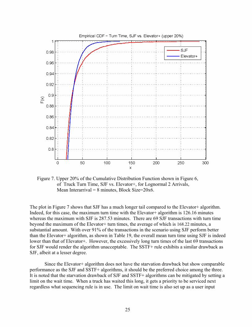
Figure 7. Upper 20% of the Cumulative Distribution Function shown in Figure 6, of Truck Turn Time, SJF vs. Elevator+, for Lognormal 2 Arrivals,

Mean Interarrival = 8 minutes, Block Size=20x6.

The plot in Figure 7 shows that SJF has a much longer tail compared to the Elevator+ algorithm. Indeed, for this case, the maximum turn time with the Elevator+ algorithm is 126.16 minutes whereas the maximum with SJF is 287.53 minutes. There are 69 SJF transactions with turn time beyond the maximum of the Elevator+ turn times, the average of which is 168.22 minutes, a substantial amount. With over 91% of the transactions in the scenario using SJF perform better than the Elevator+ algorithm, as shown in Table 19, the overall mean turn time using SJF is indeed lower than that of Elevator+. However, the excessively long turn times of the last 69 transactions for SJF would render the algorithm unacceptable. The SSTF+ rule exhibits a similar drawback as SJF, albeit at a lesser degree.

Since the Elevator+ algorithm does not have the starvation drawback but show comparable performance as the SJF and SSTF+ algorithms, it should be the preferred choice among the three. It is noted that the starvation drawback of SJF and SSTF+ algorithms can be mitigated by setting a limit on the wait time. When a truck has waited this long, it gets a priority to be serviced next regardless what sequencing rule is in use. The limit on wait time is also set up as a user input

25

parameter on the graphical user interface.Table 19: Comparison of SJF and Elevator+ Turn Time Distributions

Percentile Turn Time (in miuntes) SJF Elevator+

10% 3.97 4.20 20% 5.36 5.86 30% 6.58 7.34 40% 7.84 8.95 50% 9.33 10.81 60% 11.14 13.04 70% 13.82 16.48 80% 18.37 21.33 90% 28.94 30.00

91.73% 32.53 32.53 95% 43.91 39.14 99% 91.26 60.18 100% 287.53 126.16 Range 1.05‐287.53 1.02‐126.16 Mean 14.53 14.63

EFFECTS OF APPOINTMENTS ON CONTAINER DELIVERY

At the end of a workday, marine terminals often rearrange container storage areas in preparation for new shipment of containers as well as new requests for pickup the next day. Two schemes for the rearrangement may be possible: (1) rearrange the remaining containers from the last shipment into a concentrated area to make room for new containers from new shipments, and (2) rearrange the remaining containers from the last shipment to minimize yard height. Scheme (2) may be furthered specified for how the heights are reduced, e.g., (a) each stack of the original heights of 3-4-5-5-4-3 reduced by the same amount to, say, 1-2-3-3-2-1; or (b) all stacks reduced to the same low-rise stacks, say, 2-2-2-2-2-2. When appointments are required for container pickups, the information about which containers will be needed for pickup the next day will be extremely useful in such a rearrangement. Packing needed containers into smaller blocks has the benefit of reduced mean seek time and mean lift time, thereby resulting in smaller mean turn time. Schemes (2a) and (2b) make sense in situations where lift times overshadow seek times, which occur when many deliveries take place from deep stacks. Sgourides and Angelides in [20] considered a minimum yard height reshuffling scheme (i.e., fill every slot in the yard before forming a second container tier.) Such a scheme obviously is space intensive. With appointments and the knowledge of which containers will be needed for next day, the containers may be reshuffled so that those requested through the appointments are stacked on top of those that are not, thus getting the benefit of minimum yard height stacking without the excessive space requirement.

To investigate the effect on mean turn time for container delivery using these three reshuffling schemes based on data provided through advance appointments, we conducted a second set of simulation experiments, with the same parameters as before, except the block configurations are defined as below:

26

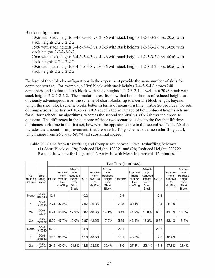
Block configuration = 10x6 with stack heights 3-4-5-5-4-3 vs. 20x6 with stack heights 1-2-3-3-2-1 vs. 20x6 with stack heights 2-2-2-2-2-2, 15x6 with stack heights 3-4-5-5-4-3 vs. 30x6 with stack heights 1-2-3-3-2-1 vs. 30x6 with stack heights 2-2-2-2-2-2, 20x6 with stack heights 3-4-5-5-4-3 vs. 40x6 with stack heights 1-2-3-3-2-1 vs. 40x6 with stack heights 2-2-2-2-2-2, 30x6 with stack heights 3-4-5-5-4-3 vs. 60x6 with stack heights 1-2-3-3-2-1 vs. 60x6 with stack heights 2-2-2-2-2-2

Each set of three block configurations in the experiment provide the same number of slots for container storage. For example, a 10x6 block with stack heights 3-4-5-5-4-3 stores 240 containers, and so does a 20x6 block with stack heights 1-2-3-3-2-1 as well as a 20x6 block with stack heights 2-2-2-2-2-2. The simulation results show that both schemes of reduced heights are obviously advantageous over the scheme of short blocks, up to a certain block length, beyond which the short block scheme works better in terms of mean turn time. Table 20 provides two sets of comparisons: the first set 10x6 vs. 20x6 reveals the advantage of both reduced heights scheme for all four scheduling algorithms, whereas the second set 30x6 vs. 60x6 shows the opposite outcome. The difference in the outcome of these two scenarios is due to the fact that lift time dominates seek time in the first set, however, the opposite is true in the second set. Table 20 also includes the amount of improvements that these reshuffling schemes over no reshuffling at all, which range from 26.2% to 68.7%, all substantial indeed.

Table 20: Gains from Reshuffling and Comparison between Two Reshuffling Schemes: (1) Short Block vs. (2a) Reduced Heights 123321 and (2b) Reduced Heights 222222. Results shown are for Lognormal 2 Arrivals, with Mean Interarrival=12 minutes.

Re-shuffling Scheme

Block Config-uration

Turn Time (in minutes)

FCFS

Improve -ment

over No Re-

shuffling

Advant-age

Reduced Height over Short Block

SJF

Improve-ment

over No Re-

shuffling

Advant-age


Elevator+

Improve-ment

over No Re-

shuffling

Advant-age


SSTF+

Improve-ment

over No Re-

shuffling

Advant-age


None 20x6 345543 12.4 10.2 10.4 10.3

1 10x6 345543 7.74 37.8% 7.07 30.8% 7.28 30.1% 7.34 28.9%

2a 20x6 123321 6.74 45.8% 12.9% 6.07 40.6% 14.1% 6.13 41.2% 15.8% 6.06 41.3% 15.8%

2b 20x6 222222 6.50 47.7% 16.0% 5.87 42.6% 17.0% 5.95 42.9% 18.3% 5.87 43.1% 18.3%

None 60x6 345543 57.0 21.8 22.1 21.6

1 30x6 345543 17.8 68.7% 13.0 40.5% 13.1 40.6% 12.8 40.9%

2a 60x6 123321 34.2 40.0% -91.8% 15.6 28.3% -20.4% 16.0 27.3% -22.4% 15.6 27.8% -22.4%

27

2b 60x6 222222 35.8 37.2% -100.5% 15.9 27.2% -22.3% 16.3 26.2% -24.3% 15.8 27.0% -24.3%

It should be noted that the improvement in turn time performance through reshuffling shown in Table 20 is based on only one-day advance appointments for pickup. Some terminals in the LA/LB ports implemented hourly appointments for import cargo pickups. Such refined appointment data should, in theory, enable terminal operators to arrange containers in such a way to minimize delivery time. However, the rate of appointment utilization at the LA/LB ports was found to be low, and kept appointments as a share of all import moves were even lower, according to an extensive study by Giuliano and O’Brien [3]. The enforcement of appointments appears to be a more complex issue than what one might expect. One resistance to using appointments by trucking companies as well as individual truck owners/operators is the fact or perception that such appointments are difficult to keep due to traffic unpredictability on the roadways in the metropolitan Los Angeles area. Results in Table 20 show that even a rudimentary one-day advance appointment system can lead to significant gains in turn time performance. Therefore, terminals may not need to be so concerned about enforcing appointments to the hour. What may be more important is how the appointment information is used for providing service. Hourly appointments can still be used to help even out load during peak operating hours. Those that have good track record in keeping their appointments can get their cargos in the most efficient manner, either on wheels, or from the most accessible locations on the yard stacks. Those of unknown quality in terms of keeping appointments will still have their containers delivered from a more concentrated area based on the appointment data, thereby resulting in an improvement of the overall performance nonetheless.

CONCLUSIONS

The Ports of Los Angeles and Long Beach have experienced remarkable growth during the past decade as a result of economic boom in the Pacific Rim countries. Marine terminals in these ports are under tremendous pressure to improve their productivity to meet demands, reduce costs, as well as mitigate problems that naturally accompany growth, including traffic congestion and air pollution. Many efforts spanning from technology adoption, to operational changes as well as legislative mandates have been undertaken towards the goal of such improvements.

The adoption of technologies such as optical character recognition (OCR) and GPS helps streamline gate entry of trucks and cargo tracking. California Assembly Bill 2650 allows terminal operators to avoid fines for trucks idling more than 30 minutes while waiting to enter the terminal gate by either extending gate hours or implementing an appointment system. The majority of the terminals in the twin ports have adopted some form of an appointment system, though with low rates of utilization and uncertain impact on reducing queuing at terminal gates [3].

Some skeptics of the potential benefits of appointments believe that “the most promising option for improving productivity is technology” and its efficient use. Technologies indeed can have great bearing on productivity gains. One way we believe technologies that support automatic cargo tracking and communications with the terminal’s computer and database system can be further used to great potential benefits. Specifically, we investigated in this study the potential gains with more intelligent scheduling of container deliveries to over-the-road trucks from import

28

yard stacks by taking advantage of the dynamic information that automatic cargo tracking technologies provide. Our findings are summarized as follows:

• The rapid growth in freight traffic at the twin ports results in increased need for stacking containers and grounded delivery. The need for more efficient delivery of containers from yard stacks under increasing load is inevitable.

• It is feasible to provide more intelligent sequencing for the container delivery, given the adoption of technology such as dGPS and RFID. These technologies enable instantaneous recording and dynamically relaying of the arrivals of trucks as well as the locations of the needed containers to all parties involved in providing the service. These capabilities in turn make it possible for the implementation of intelligent sequencing rules that can take advantage of such dynamic information.

• Intelligent sequencing rules need not be complex. Simple heuristics such as SJF, SSTF+, and Elevator+ can be very effective in reducing average truck turn time as well as queue size.

• Both SJF and SSTF+ have a drawback of starvation (some jobs may be continuously delayed by new arrivals), though the drawback can be mitigated by setting a limit on the wait time beyond which a truck will get serviced next regardless of the sequencing rule. The Elevator+ algorithm has no such deficiency and exhibits comparable performance, thus should be preferable.

• Appointment systems allow terminals to reshuffle containers booked for the next day in a concentrated area to keep blocks to be serviced small. Even with the most rudimentary system of one-day advance appointments, terminals would be able to perform sufficient amount of reshuffling to enable more efficient deliveries. This finding should help alleviate concerns of terminal operators, trucking companies and individual truck owners/operators that appointments are hard to keep under traffic conditions in the metropolitan Los Angeles area, thereby making it more likely for them to embrace the appointment systems. Which of the two schemes of reshuffling (short vs. flat block) works better depends on the relative quantity of seek time and lift time for the container delivery.

• The simulation program we have developed is sufficiently flexible to allow users to input parameters that reflect future condition of their terminal’s operations and determine if alternative sequencing rules for container deliveries warrant implementation.

• The concepts developed and the findings obtained in this project may easily be adopted in a simulation test bed developed in the METRANS project 05-11 by Ioannou and Chassiakos [5].

REFERENCES

[1] Blackburn. Daniel. (2006) Letter of ROP Research.

[2] Blackburn. Daniel et al. (2006) A series of email messages regarding “RTG JOB LIST promotion.”

[3] Genevieve Giuliano and Tom O'Brien (2007) Reducing Port Related Truck Emissions: The Terminal Gate Appointment Systems at the Ports of Los Angeles and Long Beach. Transportation Research Part D, 12, 460-473.

29

[4] Kim K.H., Lee K.M, Hwang H. (2003) Sequencing delivery and receiving operations for yard cranes in port container terminals. International Journal of Production Economics 84(3): 283-292.

[5] Ioannou P. and Chassiakos A. (2005) Simulation Test Bed and Evaluation of Truck Movement Concepts on Terminal Eficiency and Traffic Flow. METRANS Project 05-11.

[6] James, K. and Rodriquez, L. (2007) Videotaping of RTG Operations at Container Terminal Y in the LA/LB Seaports, Oct. 2007.

[7] Jin C., Liu X. and Gao P. (2004) An Intelligent Simulation Method Based on Artificial Neural Network for Container Yard Operation. Proceedings of Advances in Neural Networks (ISNN 2004), Springer LNCS 3174, 904-911.

[8] Lam S,F., Park, J and Pruitt C. (2006) An Accurate Monitoring of Truck Waiting and Flow Time. METRANS AR 05-01.

[9] Lai, K.K. and Leung, J.W. (1996) Analysis of Yard Crane Deployment Strategies in a Container Terminal. Proceedings of ICC and IE Conference, Kyungju, South Korea, 1187-1190.

[10] Mitsubishi Heavy Industries Ltd. (2007) Container Transfer Crane Specifications. http://www.mhi.co.jp/en/products/detail/transfer_crane.html. Retrieved October 2007.

[11] Murty K., Wan Y., Liu J., Tseng M., Leung E., Lai K-K., Chiu H. (2005) Hongkong International terminals Gains Elastic Capapcity Using a Data-Intensive Decision-Support System, Interfaces 35 (1) 61-75.

[12] Nam K.-C., Kwak K.-S., and Yu M.-S. (2002). Simulation Study of Container Terminal Performance. Journal of Waterway Port Coastal and Ocean Engineering 128(3), 126-132.

[13] Ng W.C. and Mak K.L. (2004) Sequencing of Container Pickup Trucks in Container Yard Blocks. International Journal of Industrial Engineering 11(1), 82-89.

[14] Parola, F. and Sciomachen, A. (2005) Intermodal Container Flows in a Port System Network: Analysis of Possible Growth Via Simulation Models. International Journal of Production Economics 97, 75-88.

[15] Pathak P. (1995). Port facility planning using computer simulation: A case study. Port Technology Journal Archive, Edition 6, Section 8: Port Planning Construction and Maintenance, Port Technol. Int., 203–211.

[16] The Port of Los Angeles TEU Statistics (2008) http://www.portoflosangeles.org/maritime/stats.asp. Retrieved April 8, 2008.

30

http://www.portoflosangeles.org/maritime/stats.asp

http://www.mhi.co.jp/en/products/detail/transfer_crane.html

[17] The Port of Long Beach Yearly TEUs (2008) http://www.polb.com/economics/stats/yearly_teus.asp. Retrieved April 8, 2008.

[18] Rizzoli, A.E., Fornara, N., and Gambardella, L.M. (2002) A Simulation Tool for Combined Rail/Road Transport in Intermodal Terminals. Journal of Mathematics and Computers in Simulation 59 (1-3), 57-71.

[19] Ryan N. K. (1998). The Future of Maritime Facility Designs and Operations. Proc, 1998 Winter Simulation Conf., Washington, D.C. 1223–1227.

[20] Sgouridis S. and Angelides D. (2002) Simulation-Based Analysis of Handling Inbound Containers in a Terminal. Proc. 2002 Winter Simulation Conference. 1716-1724.

[21] Teorey, T.J. and Pinkerton, T.B. (1972) A Comparative Analysis of Disk Scheduling Policies. Communications of the ACM, Vol. 15, No. 3. 177-184.

[22] Wilson, Eric. (2006) Private communication.

31

http://www.polb.com/economics/stats/yearly_teus.asp

metrans project 07-12

Documents