methods -development for quantification of ozone -and
TRANSCRIPT

- middot
w -middot - bull bull bull bull bull ~- bull bull lt_ middot~ middotmiddot _middot
middot_ middot~- _middot ~~-~Lr-c~- middot
- - -1f~IU -
middot
middot
Methods -Development for Quantification of Ozone -and -_Ozone Precursormiddot Transport i_n
middot California
METHODS DEVELOPMENT FOR QUANTIFICATION OF OZONE AND OZONE PRECURSOR
TRANSPORT IN CALIFORNIA
Final Report
Contract No A932-143
Prepared for
California Air Resources Board Research Division
2020 L Street Sacramento California 95814
Prepared by
Paul T Roberts Hilary H Main Lyle R Chinkin
Stefan F Musarra
Sonoma Technology Inc 5510 Skylane Blvd Suite 101
Santa Rosa California 95403 1 083
and
Till E Stoeckenius
Systems Applications International 101 Lucas Valley Road
San Rafael California 94903
JULY 1993
ABSTRACT
This project addresses the California Clean Air Act requirement to assess the relative contribution of upwind pollutants to violations of the state ozone standard in downwind areas The objectives of the project were
bull To develop data analysis methods to quantify the contribution of upwindemissions to downwind ozone concentrations
bull To apply those methods to the transport of pollutants from the San Francisco Bay Area and the San Joaquin Valley Air Basins plus the Lower Sacramento Valley to receptor sites in the Upper Sacramento Valley and
bull To recommend the best methods to use for the Upper Sacramento Valley
The project results should improve future analysis modeling and emission control efforts
This project has included amiddotnumber of tasks such as preliminaryplanning a field measurement study and subsequent data analyses A number of reports have documented the data collected during the field study This report covers the data analysis portion of the project and includes information on important issues when considering pollutant transport a discussion of the data analysis methods used in this project including the method limitations a presentation of the results of applying the various methods comparisons and evaluations of the results and a discussion of project conclusions and of recommendations for future applications
The data analysis methods which could be applied in future applicationsfor the Upper Sac include transport paths and precursor contribution estimates using surface and aloft trajectories 2-D pollutant flux estimates ozonetracer regressions and analyses of unique signatures of VOC species and tracers of opportunity In addition air flow patterns should be characterized as a basis for any of the other methods At least two of the methods should be applied at the same time in order to strengthen the results For future applications the following recommendations are made
bull If limited to the use of existing monitoring then only one method that we studied is possible precursor contribution estim~tes for NOx and ROG using surface trajectories This method is only applicable to those Upper Sac receptors which are influenced by same-day surface transport
bull New hourly VOC-speciation monitoring will be needed in the Sacramento area to meet EPAs PAMS (Photochemical Assessment Monitoring Stations)requirements If a similar monitor is also installed at one or more Upper Sac receptors then VOC-signature analyses could be performed to quantify precursor transport This technique enables the potentialidentification of the source of the air parcel based on the VOC signature if these signatures are observed to differ amoung source regions
ii
bull Based on analyses in this study if additional measurements can be taken such that 2-D flux plane and VOC-signature analysis methods can be employed the combination of these techniques provides the most reliable quantification of ozone and ozone precursors (Intensive field measurements on potential transport days would be required) These methods are reliable because they are based on calculations and comparisons using physical parameters such as wind speed wind direction ozone concentration and VOC speciation rather than relying on purely statistically related param~ters which may not be physicallyrelated such as the timing of ozone peaks
iii
ACKNOWLEDGMENTS
The work described in this report was funded by the California Air Resources Board (ARB) The project officer was Mr Chuck Bennett of the Research Division of the ARB his suggestions and comments were very useful and are greatly appreciated Mr Steve Gauze of the Technical SupportDivision of the ARB also provided useful suggestions and comments throughoutthe project
We would also like to thank the following individuals for their helpduring this project
bull The following people and organizations for collecting field data for this project
- Mr Joel OCamb STI for preparing the air quality aircraft for flying in the aircraft to collect the aircraft data and for doingmuch of the aircraft data processing and report writing
- Ms Juanita Gardner STI for writing the aircraft data processingsoftware and for processing the data
- Mr Rob Williams STI and Mr Steve Church STI also helped prepare the aircraft for sampling and assisted with operations in the field
- Mr Jerry Anderson STI performed some of the calibrations of the monitors operated on the aircraft We greatly appreciate his care and diligence during these calibrations his efforts to tie the aircraft calibrations to other calibrations that were performedduring the summer of 1990 and his help during review of the processed data
- Ms Elaine Prins STI and Mr Joe Newmann directed the upper-airmeteorological measurements Mr Lin Lindsey STI and Dr Rolland Hauser of California State University at Chico provided guidance and assistance during the field measurements
- Mr Cliff Garratt Ms Tracey Johnson and Ms Gail Nottingham of Chico and Mr Xo Larimer of the ARB performed the upper-airmeteorological soundings
- Mr Jeff Prouty STI wrote most of the software used to processand review the upper-air meteorological data
- Mt William R Knuth STI in cooperation with Mr Chuck Bennett and the Meteorology Section of the ARB provided daily forecasts for the field measurements
- Mr Steve Quon of Tracer Technologies managed the tracer field program and the ozone monitoring at Sutter Buttes and Maxwell
iv
- Dr Rei Rasmussen of the Oregon Graduate Institute provided the voe sampling equipment and performed the laboratory analyses for voe species and tracers of opportunity He went to great lengths to provide VOC species and tracers-of-opportunity results for all collected samples
- Dr Ted B Smith for consulting on the tracer experiment design and the forecasting criteria
bull Ms LuAnn Gardner of Systems Applications International (SAi) for helping to prepare the emissions inventory for this project
bull Ms Sandy Barger Ms Sue Hynek Ms Claire Romero and Ms Barbara Austin for helping to prepare this report
bull The following people and organizations for providing data for this project
- Mr David Young of the Sacramento Area Council of Governments - Mr Steve Quon of Tracer Technologies - Mr Steve Gauze Mr Rich Hackney Mr Chuck Bennett Mr Xo
Larimer and Mr Dennis King of the ARB - Or Rolland Hauser of California State University at Chico - Mr Tom Cushman of Weather Network Inc - The National Weather Service - The National Ocean Buoy Center - The San Joaquin Valley Air Quality Study and AUSPEX
This report was submitted in fulfillment of the ARB Contract A932-143 Methods Development for Quantification of Ozone Transport for California by Sonoma Technology Inc under the sponsorship of the California Air Resources Board Work was completed as of January 20 1993
V
DISCLAIMER
The statements and conclusions in this report are those of themiddot contractor and not necessarily those of the California Air Resources Board The mention of commercial products their source or their use in connection with material reported herein is not to be construed as either an actual or implied endorsement of such products
vi
TABLE OF CONTENTS
Section
ABSTRACT bull ii ACKNOWLEDGMENTS bullbullbull iv DISCLAIMER bullbullbull vi LIST OF FIGURES X LIST OF TABLES bull xv
I INTRODUCTION bull bull bull bull 1-1 II PROJECT RATIONALE AND OBJECTIVES 1-1 12 TECHNICAL APPROACH bullbull 1-2 13 SUMMARY OF TRANSPORT METHODS USED DURING THIS PROJECT 1-6
131 Flow Characteristics bullbullbullbullbullbull 1-7 132 Statistical Analyses bullbullbullbullbull 1-7 133 Trajectory-based Methods bullbullbullbullbull 1-8 134 Pollutant Flux Estimates bull 1-8 135 voe Species and Tracers-of-Opportunity Analysis
Methods bull bull 1-9 136 Tracer Analysis Methods bull 1-9
14 SUMMARY OF OVERALL PROJECT CONCLUSIONS 1-9 15 SUMMARY OF RECOMMENDATIONS FOR FUTURE METHODS APPLICATIONS
IN THE UPPER SACRAMENTO VALLEY 1-11 16 REPORT CONTENTS 1-12
2 FIELD STUDY OVERVIEW middot 2-1 21 INTRODUCTION AND BACKGROUND 2-1 22 FIELD STUDY COMPONENTS 2-2
221 Air Quality Monitoring Network 2-2 222 Meteorological Monitoring Network 2-2 223 Air Quality Aircraft bull 2-3 224 Perfluorocarbon Tracer Tests 2-3 225 Field Management bull 2-9
3 TECHNICAL ISSUES 3-1 31 OZONE FORMATION 3-1 32 PRECURSOR EMISSIONS 3-2 33 GEOGRAPHICAL SETTING AND RESULTING METEOROLOGICAL ISSUES 3-2 34 OTHER ISSUES 3-3 35 AVAILABILITY OF SURFACE AND ALOFT METEOROLOGICAL AND AIR
QUALITY DATA 3-4 36 RELIABILITY OF FINDINGS 3-4
4 FLOW CHARACTERISTICS bull 4-1 41 TYPICAL AIR FLOW PATTERNS IN THE SACRAMENTO VALLEY 4-1 42 DESCRIPTIONS OF FLOW PATTERNS AND MAXIMUM OZONE
CONCENTRATIONS DURING INTENSIVE MEASUREMENT PERIODS 4-5 421 July 10-13 1990 Episode bull bull 4-5 422 August 10-12 1990 Episode bull bull bull 4-8
43 SUMMARY OF CHARACTERISTICS DURING 1990 INTENSIVE SAMPLING 4-8
vii
TABLE OF CONTENTS (Continued)
Section
5 STATISTICAL ANALYSIS OF OZONE AND METEOROLOGICAL DATA 51 DIURNAL OZONE CONCENTRATION PATTERNS 52 CORRELATION ANALYSIS bull 53 STEP-WISE REGRESSION ANALYSIS 54 CONCLUSIONS bull ~ bull
6 PRECURSOR CONTRIBUTION ESTIMATES USING TRAJECTORY METHODS 61 TRANSPORT-PATH ANALYSES
611 Summary of Trajectory Methods 612 Trajectory Results Using Surface Data 613 Trajectory Results Using Aloft Data
62 PRECURSOR CONTRIBUTION ESTIMATES 621 Summary of Emissions Inventory Methods 622 Summary of Precursor Contribution Estimate Method 623 Precursor Contribution Estimates
63 ANALYSIS RESULTS USING TRAJECTORY METHODS 64 RECOMMENDATIONS
7 POLLUTANT FLUX ESTIMATES 71 SIMPLE OZONE AND NOx FLUX PLOTS 72 OZONE AND NOx FLUX ESTIMATES
721 Flux Plane Definition 722 Data Preparation 723 Flux Estimation Results 724 Summary of Flux Calculation Assumptions 725 Discussion of Results 726 Applications of the Method to Other Data
73 SUTTER BUTTES METEOROLOGICAL AND AIR QUALITY MEASUREMENTS 731 Meteorological Measurement Comparisons 732 Air Quality Measurement Comparisons
74 CONCLUSIONS AND RECOMMENDATIONS
8 ANALYSES USING voe SPECIES AND TRACERS OF OPPORTUNITY 81 OBJECTIVES 82 AVAILABLE DATA bull 83 METEOROLOGICAL SETTING 84 UNIQUE SOURCE AREA SIGNATURES bull 85 COMPARISON OF UPWIND SIGNATURES TO UPPER SACRAMENTO VALLEY
SAMPLES 86 AGE OF AIR PARCELS 87 STATISTICAL ANALYSES bull middotbullbullbull 88 CONCLUSIONS AND RECOMMENDATIONS bull bull bull bull
881 Application of Methods to Upper Sacramento ValleyData bull bull
882 Application of Methods to Other Data
9 SACRAMENTO VALLEY TRANSPORT STUDY TRACER EXPERIMENTS bullbull 91 TRACER STUDY DESIGN
Page
5-1 5-1
5-11 5-14 5-14
6-1 6-1 6-1 6-3 6-8
6-18 6-18 6-19 6-26 6-36 6-39
7-1 7-1 7-5 7-9 7-9
7-10 7-14 7-15 7-15 7-16 7-16 7-20 7-22
8-1 8-1 8-1 8-2 8-4
8-10 8-10 8-15 8-16
8-16 8-17
9-1 9-1
viii
TABLE OF CONTENTS (Concluded)
Section Page
92 TRACER STUDY RESULTS 9-3 92l July 19-13 1990- Tracer Study Results 9-3 922 August 10-12 1990 Tracer Study Results 9-6
93 CLIMATOLOGICAL COMPARISONS bull 9-6 94 IMPLICATIONS FOR OZONE AND PRECURSOR TRANSPORT 9-10 95 OZONETRACER REGRESSIONS ANALYSIS RESULTS 9-10 96 TRACER STUDY RESULTS AND RECOMMENDATIONS FOR FUTURE WORK 9-16
10 CONCLUSIONS AND RECOMMENDATIONS bull 10-1 101 CONCLUSIONS AND RECOMMENDATIONS ON EACH METHOD 10-1 102 COMPARISON OF METHODS RESULTS 10-10 103 OVERALL PROJECT CONCLUSIONS AND RECOMMENDATIONS 10-11
11 REFERENCES bullbull 11-1
APPENDIX A ARB AIR FLOW CHARTS FOR JULY 10-13 1990 AND AUGUST 10-12 1990 A-1
APPENDIX B SURFACE METEOROLOGICAL MEASUREMENT LOCATIONS USED FOR UPPER SACRAMENTO VALLEY TRAJECTORIES 8-1
APPENDIX C ESTIMATED RELATIVE OZONE FLUX OZONE CONCENTRATION AND RESULTANT WIND SPEED AT SUTTER BUTTES AND LAMBIE ROAD JUNE 21 - AUGUST 19 1990 C-1
APPENDIX D voe AND EXOTICS DATA SUMMARY FROM THE UPPER SACRAMENTO VALLEY TRANSPORT STUDY 0-1
APPENDIX E CORRECTED OZONE CONCENTRATIONS FOR RED BLUFF FOR AUGUST 5 - AUGUST 15 1990 E-1
ix
LIST OF FIGURES
Figure Page
1-1 Map of Northern California showing the Upper Sacramento Valleythe Broader Sacramento Area (prior to September 1992) the San Francisco Bay Area and selected sampling sites 1-3
1-2 Map of Northern California showing the Upper Sacramento Valleythe Broader Sacramento Area (after September 1992) the middot San Francisco Bay Area and selected sampling sites 1-4
2-1 Example STI aircraft flight pattern on first afternoon of intensive sampling Flight 605 on August 10 1990 1348-1733 PDT 2-4
2-2 Example STI aircraft morning flight during intensive samplingFlight 606 on August 11 1990 0535-0834 PDT bull 2-6
2-3 Example STI aircraft afternoon flight during intensive samplingFlight 607 on August 11 1990 1328-1627 PDT 2-7
2-4 Map of tracer release aircraft sampling sites
and ground sampling 2-8
4-1 Sacramento Valley air flow pattern types 4-2
4-2 Bay Area air flow pattern types 4-4
5-1 Diurnal profiles of hourly ozone concentrations averaged over all potential transport days for Burney compared with similar plotsfor days not in the potent i a 1 transport group bull bull bull 5-3
5-2 Diurnal profiles of hourly ozone concentrations averaged over all potential transport days for Redding compared with similar plotsfor days not in the potential transport group 5-3
5-3 Diurnal profiles of hourly ozone concentrations averaged over all potential transport days for Red Bluff compared with similar plotsfor days not in the potential trinsport group 5-4
5-4 Diurnal profiles of hourly ozone concentrations averaged over all potential transport days for Chico compared with similar plots for days not in the potential transport group bull bull 5-4
5-5 Diurnal profiles of hourly ozone concentrations averaged over all potential transport days for Willows compared with similar plotsfor days not in the potential transport group bullbullbullbullbullbullbullbull 5-5
5-6 Diurnal profiles of hourly ozone concentrations averaged over all potential transport days for Maxwell compared with similar plotsfor days not in the potential transport group 5-5
X
LIST OF FIGURES (Continued)
Figure Page
5-7 Diurnal profiles of hourly ozone concentrations averaged over all potential transport days for Sutter Buttes compared with similar plots for days not in the potential transport group 5-6
5-8 Diurnal profiles of hourly ozone concentrations averaged over all potential transport days for Yuba City compared with similar plots for days not in the potential transport group bull 5-6
5-9 Diurnal profiles of hourly ozone concentrations averaged over all potential transport days for Tyndall compared with similar plotsfor days not in the potential transport group 5-7
5-10 Diurnal profiles of hourly ozone concentrations averaged over all potential transport days for West Nicolaus compared with similar plots for days not in the potential transport group 5-7
5-11 Diurnal profiles of hourly ozone concentrations averaged over all potential transport days for Pleasant Grove compared with similar plots for days not in the potential transport group 5-8
5-12 Diurnal profiles of hourly ozone concentrations averaged over all potential transport days for North Highlands compared with similar plots for days not in the potential transport group 5-8
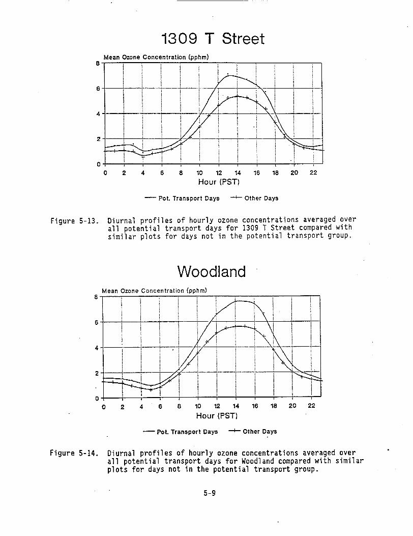
5-13 Diurnal profiles of hourly ozone concentrations averaged over all potential transport days for 1309 T Street compared with similar plots for days not in the potential transport group 5-9
5-14 Diurnal profiles of hourly ozone concentrations averaged over all potential transport days for Woodland compared with similar plots for days not in the potential transport group 5-9
6-1 Map showing surface wind sites for Upper Sacramento Valley trajectories 6-4
6-2 Surface back trajectories from Red Bluff Redding and Chico on June 26 1987 beginning at 1600 PST 6-5
6-3 Surface back trajectories from Red Bluff Redding and Chico on July 14 and 15 1987 beginning at 1200 PST bull 6-6
6-4 Surface back trajectories from Red Bluff Redding and Chico on August 7 1987 beginning at 1600 PST and on August 8 1987 beginning at 1200 PST bull bull bull bull 6-7
6-5 Surface back trajectory from Chico on August 5 1989 beginning at 1600 PST 6-10
xi
LIST OF FIGURES (Continued)
Figure Page
6-6 Aloft back trajectories from Chico on August 5 1989 beginning at 1600 PST at a) 400 meters and b) 800 meters bull bull bull bull 6-11
6-7 Hourly ozone concentrations at a) Redding and (b) Chico on August 7-9 1990 bullbullbullbullbullbullbullbull 6-12
6-8 Surface back trajectories from Redding on August 7 1990 beginning at a) 1200 b) 1400 and c) 1600 PST bull 6-14
6-9 Aloft 400 m back trajectory from Redding on August 7 1990 beginning at 1200 PST and 400 m forward trajectory from Howe Park on August 6 1990 beginning at 1600 PST 6-15
6-10 Surface back trajectories from Redding and Chico on August 8 1990 beginning at 1200 PST bull 6-16
6-11 Aloft 400 m back trajectories from Chico on August 8 1990 beginning at 1200 PST bullbullbullbullbullbullbull 6-17
6-12 Illustration of precursor accumulation geometry along a trajectory path bullbull
6-13 Example of ROG accumulation along a surface trajectory path(a) without reaction and (b) with reaction 6-22
6-14 ROG emissions contribution estimates (a) without reaction and (b) with reaction for surface 400 meter and 800 meter back trajectories from Chico on August 5 1989 (average of three trajectories at 1200 1400 and 1600 PST) bullbullbull 6-24
6-15 NOx emissions contribution estimates (a) without reaction and (b) with reaction for surface 400 meter and 800 meter back trajectories from Chico on August 5 1989 (average of three trajectories at 1200 1400 and 1600 PST) bull 6-25
6-16 Average precursor contribution estimates with reaction for 21 surface back trajectories from Chico on seven daysduring 1989 bull bull bull bull bull bull bull bull bull bull bull bull bull 6-27
6-17 Average precursor contribution estimates for (a) local and transport exceedance days at Redding using surface trajectories (18 exceedance days at either Redding or Anderson during 1987) 6-30
6-18 Average precursor contribution estimates for (a) local and (b) transport days at Red Bluff using surface trajectories(18 exceedance days at either Redding or Anderson during 1987) 6-31
xii
LIST OF FIGURES (Continued)
Figure Page
6-19 Average precursor contribution estimates for a local and (b transport days at Chico using surface trajectories(18 exceedance days at either Redding or Anderson during 1987) 6-32
6-20 Average precursor contribution estimates for transport exceedance days at Chico using surface trajectories (six exceedance days at Chico during 1987 and 1988 bull bull 6-33
6-21 Surface back trajectories from Arbuckle and Willows bn October 7 1987 beginning at 1400 PST 6-34
6-22 Average precursor contribution estimates for October 7 (a) Arbuckle and (b) Willows using surface trajectories
1987 at 6-35
7-1 Three flux planes investigated in Section 7 7-2
7-2 (a) Estimated relative ozone flux and (b) ozone concentration and resultant wind speed at Sutter Buttes July 11-13 1990 7-3
7-3 (a) Estimated relative ozone flux and (b ozone concentration and resultant wind speed at Lambie Road July 11-13 1990 7-4
7-4 (a) Estimated relative NOx flux and (b NOx concentration and resultant wind speed at Lambie Road July 10-14 1990 7-6
7-5 (a) Estimated relative ozone flux and (b) ozone concentration resultant wind speed at Sutter Buttes August 10-12 1990
and 7-7
7-6 (a Estimated relative ozone flux and (b) ozone concentration resultant wind speed at Lambie Road August 10-12 1990
and 7-8
7-7 (a) Ozone concentrations (b) wind speed and (c) ozone flux aloft on August 10 1990 at about 1600 PDT 7-12
7-8 (a) NOx concentrations and (b NOx flux aloft on August 10 at about 1600 PDT
1990 7-13
7-9 Comparisonof surface wind directions at Sutter Buttes with aloft wind direction at (a Maxwell and (b North Yuba 7-19
7-10 Comparison of Sutter Buttes surface ozone concentrations with (a nearby aloft and (b) Maxwell surface ozone bull 7-23
7-11 Diurnal ozone concentrations for Sutter Buttes during July -September (1989-1990 on (a all days and (b days with ozone peaks greater than 9 pphm 7-24
xiii
LIST OF FIGURES Concluded)
Figure Page
8-1 Comparison of Point Reyes and Travis a) VOC and b) exotics data in 1990 middot 8-7
8-2 Comparison of Travis and Richmond (a) voe and b) exotics data in 1990 8-8
8-3 The composition of two a) voe and (b) exotics samples collected downwind of the Broader Sacramento Area at Folsom and Auburn 8-9
8-4 Comparison of a) VOC and b) exotics signatures at North Yuba Folsom and Travis bull bull 8-11
8-5 Comparison of a) voe and (b) exotics signatures at Chico Folsom and Travis 8-12
8-6 Comparison of (a) voe and (b) exotics signatures at ReddingFolsom and Travis bullbullbullbull 8-13
9-1 Tracer release aircraft and surface sampling locations 9-2
9-2 July 11th afternoon release 9-4
9-3 July 12th morning release 9-5
9-4 August 10th afternoon release 9-7
9-5 August 11th morning release 9-8
9-6 Expected tracer observations from climatological flow pattern 9-9
9-7 Ozone and Lambie Road tracer concentrations measured on August 11 1990 at the surface at (a) Red Bluff ~nd (b) Redding 9-11
9-8 Ozone and Lambie Road tracer concentrations measured on August 11 1990 at the surface and aloft at (a) Red Bluff and (b) Redding bull 9-12
9-9 Ozonetracer regression results using August 10-12 1990 data from Redding bull bull 9-13
9-10 Hypothetical example of ozonetracer regression at an UpperSacramento Valley monitoring site for a) tracer representingthe Broader Sacramento Area and (b) tracer representing the SF Bay Area bull bull bull bull bull bull 9-15
xiv
LIST OF TABLES
Table Page
2-1 Summary of STI aircraft sampling locations during the 1990 UpperSacramento Transport Study bullbullbullbull ~ bull bull bull bull bull bull 2-5
4-1 Percentage of occurrence of SF Bay Area air flow types during the summer bull bull bull 4-3
4-2 Peak ozone concentrations (9 pphm or above) measured at ReddingRed Bluff Chico Sutter Buttes Lower Sacramento Valley and San Francisco Bay Areamiddotduring July and August of 1990 4-6
5-1 Dates of potential transport (ie with daily maximum ozone gt = 95 pphm) at Redding Chico or Red Bluff 5-2
5-2 Number of non-missing hourly ozone values (1200 to 1800 PST) on 1990 potential transport days (see Table 5-1) by site and transport category bull 5-10
5-3 Station correlations for Sacramento ozone sites Pearson correlation coefficients Probgt IRI under Ho Rho=O number of observations bull 5-12
5-4 Correlation of daily maximum ozone concentrations Pearson correlation coefficients Probgt IRI under Ho Rho=O number of observations bull 5-13
5-5 Summary of simple linear regression for daily maximum ozone at selected sites for each candidate regression variable 5-15
5-6 Summary of forward step-wise regression analysis using dailymaximum ozone as the dependent variable and regressors 5-16
6-1 Redding or Anderson exceedance days during 1987 selected for trajectory analysis and maximum ozone concentrations 6-28
6-2 Classification of 1987 Redding or Anderson exceedance days as transport or local at Redding Red Bluff and Chico 6-28
7-1 Data available for flux calculations along the Upper Sacramento Valley flux plane on August 10 1990 bull bull bull bull bull 7-10
7-2 Surface wind speeds and directions at Maxwell Sutter Buttesmiddot and North Yuba and aloft winds at Maxwell and North Yuba 7-17
7-3 Results of linear regressions between surface and upper air wind speed and direction measured at Maxwell North Yuba and Sutter Buttes 7-18
xv
LIST OF TABLES (Concluded)
Table Page
7-4 Ozone concentrations measured aloft near Sutter Buttes at the surface monitoring station atop Sutter Buttes and at the surface at Maxwel 1 bull bull 7-21
7-5 Results of linear regressions between surface and aircraft ozone concentrations measured at Sutter Buttes and Maxwell 7-22
8-1 List of exotic species names background concentrations and sources 8-3
8-2 Clean air criteria for hydrocarbon samples 8-5
8-3 Application of clean air criteria to Upper Sacramento Valley and source signature hydrocarbon samples 8-14
B-1 Wind Sites for Upper Sacramento Valley trajectories including site number (See Figure 6-1) and UTM coordinates 8-2
D-1 Major voe species groups concentrations for each sample collected during the Upper Sacramento Valley Transport study 0-2
D-2 Definition of validation codes used to flag Upper Sacramento Valley voe and exotics samples D-4
D-3 Exotic species concentrations for each sample collected during the Upper Sacramento Valley Transport study 0-5
D-4 Exotic species concentrations of samples collected at Point Reyesand Richmond during the San Joaquin ValleyAUSPEX study D-8
xvi
1 INTRODUCTION
11 PROJECT RATIONALE AND OBJECTIVES
The State of California has been divided into 14 air basins Air pollution control districts or air quality management districts in each basin have been concerned with the control of local emissions and the impact of those emissions on pollutant concentrations in their basin Altho~gh many of the basin boundaries were established with terrain features in mind prevailing wind patterns in the state still transport pollutants from one basin to another This effect has been clearly_demonstrated on a number of occasions through the use of tracer releases (see for example Smith et al 1977 Lehrman et al 1981 Smith and Shair middot1983 and Reible et al 1982)Depending on the particular scenario effective control strategies may requireemission controls in the upwind air basin the downwind air basin or both
The California Clean Air Act requires the California Air Resources Board (ARB) to assess the relative contribution of upwind pollutants to violations of the state ozone standard in the downwind areas Past transport studies in California have documented pollutant transport on specific days but have not always quantified the contribution of transported pollutants to ozone violations in the downwind area
Grid modeling may ultimately be needed in many situations to evaluate the relative effects of different control strategies However many of the interbasin transport problems in the state involve complex flow patterns with strong terrain influences which are difficult and expensive to model Limited upper-air meteorological and air quality data in many areas generally restrict the evaluation and thus the effective use of grid models In addition interbasin transport between some of the air basins does not result in significant receptor impact and thus should not receive the detailed treatment afforded by grid modeling
This project was designed to develop and apply data analysis methods to quantify the contribution of transported pollutants to ozone violations in the Upper Sacramento Valley (Upper Sac) to evaluate the results of applying the various methods and to recommend the best methods to use for the Upper Sac The project results should improve future analysis modeling and control efforts
The objectives of the project were
bull To develop data analysis methods to quantify the contribution of upwindemissions to downwind ozone concentrations
bull To apply those methods to the transport of pollutants from the San Francisco Bay Area (SF Bay Area) and the San Joaquin Valley Air Basins plus the Lower Sacramento Valley (Broader Sac) to receptor sites in the Upper Sac and
bull To recommend the best methods to use for the Upper Sac receptor area
1-1
During the period when this project was planned and carried out the Upper Sac area was defined as the counties of Shasta Tehama Glenn Butte and Colusa The upwind areas which might contribute transported pollutants to the Upper Sac area are the SF Bay Area the San Joaquin Valley Air Basin (SJVAB) and the Broader Sac Figure 1-1 is a map of the general area which shows these three areas Note that if pollutants are transported from the SF Bay Area or from the SJVAB to the Upper Sac they must first pass through the Broader Sac The natural geographicalmeteorological division between the Broader Sac and the Upper Sac is on an eastwest line at Sutter Buttes
In September 1992 the ARB modified the boundaries of the Upper Sac and Broader Sac areas (see Figure 1-2) These changes essentially moved the Broader SacUpper Sac boundary about 40 km south and added Yuba City and Marysville to the Upper Sac These changes do not match the natural geographicalmeteorological division between the two areas Future transport assessments would require measurements at different locations than those used in this project
This project has included a number of tasks including preliminaryplanning a field measurement study and subsequent data analyses A number of previous reports have documented the data collected during the field study (see Section 2 for a summary of the field study and associated references) This report covers the data analysis portion of the project and includes information on important issues when considering pollutant transport a discussion of the data analysis methods used in this project a presentation of the results of applying the various methods comparisons and evaluations of the results and a discussion of project conclusions and of recommendations for future applications
While we were performing work for this project we were also performingwork on another project on pollutant transport for the ARB (A Study to _ Determine the Nature and Extent of Ozone and Ozone Precursor Transport in Selected Areas of California Roberts et al 1992) Since pollutant transport to the Upper Sac was one of the four areas selected for study during that parallel project there was some overlap between the two projects Results of some of the work performed for the current study was included in the earlier report as well as in this one in order to present the results to the ARB as soon as possible This overlap occurs mainly in the estimation of precursor contribution estimates (see Section 6)
The rest of this section presents our technical approach a summary of the project results and our recommendations for future use of the methods applied during this project
12 TECHNICAL APPROACH
A number of issues influenced our technical approach to quantifying pollutant transport including the following The impact of pollutant transport on the ozone air quality in a downwind basin is a function of the precursor emissions in the upwind basin the losses of pollutants by deposition and reaction along the transport path the formation of ozone alongthe transport path the meteorological situation which transports and mixes
1-2
e BURNEY
e REDDING
bull RED BLUFF _
UPPER SACRAMENTO J t--t---~ VALLEY _
Figure 1-1 Map of Northern California showing the Upper Sacramento Valleythe Broader Sacramento Area (prior to September 1992) the San Francisco Bay Area and selected sampling sites All sites are shown in Figure 6-1 and listed with UTM-coordinates in Appendix B
1-3
e REDDING
bullBURNEY
e RED BLUFF
r---i____1UPPER SACRAMENTO VALLEY
~
I I l
SAN JOAQUIN VALLEY AIR
BASIN
Figure 1-2 Map of Northern California showing the Upper Sacramento Valley the Broader Sacramento Area (after September 1992) the San Francisco Bay Area and selected sampling sites All sites are shown in Figure 6-1 and listed with UTM coordinates in Appendix B
1-4
the pollutants and the local precursor emissions in the downwind basin The geography of the region often influences the potential transport between air basins and the transport path In addition the availability of surface and aloft meteorological and air quality data will determine which potential data analysis methods could be applied to quantify pollutant transport to a downwind air basin
To meet the project objectives modeling or data analysis methods could be applied For this project we applied data analysis methods using
meteorological and air quality data collected routinely or during specialstudies The issues mentioned above lead us to design a technical approachwhich relied on developing multiple methods to quantify pollutant transport
middot rather than just one or two This multi-pronged approach increased the ability of the project to meet its objectives and provided a way to evaluite middot the uncertainty or reliability of the various methods Our technical approachincluded identifying and selecting methods acquiring the data needed to applythem applying the methods and comparing and evaluating the results In addition we have analyzed the air flow characteristics in the Sacramento Valley the San Joaquin Valley and the SF Bay Area in order to provide a basic understanding of how when and where pollutant transport might occur this understanding was a useful component of all other analysis methods
First we identified and selected methods to quantify the influence of transported pollutants on downwind ozone concentrations and identified the data required by these methods The methods range from simple techniqueswhich use only routine air quality and meteorological data to more complextechniques which require special field data There was very little time between the award of the contract and the required field measurements which had to take place in the summer of 1990 in order to coincide with the extensive field measurements being taken in and near the Sacramento Valleyincluding the Sacramento Area Ozone Study (SAOS) and the San Joaquin ValleyAir Quality Study and Atmospheric Utilities Signatures Predictions and Experiments (SJVAQSAUSPEX) Thus there was not enough time before the field measurements to apply the selected methods to existing data sets and use the results to refine the field measurements
Next we planned the field measurements to acquire the data needed to apply the selected methods Some of the needed data were routinely available while other data had to be collected during an intensive field measurement program The intensive field measurement program included perfluorocarbon tracer tests aircraft and meteorological measurements aloft and speciated measurements for many volatile organic compounds (VOC) species and several tracers of opportunity (chlorofluorocarbons-CFCs) A significant data validation effort was also performed in order to prepare the field data for use in the methods application tasks A summary of the field measurement program is included in Section 2
Based on a review of meteorological and air quality data ARB staff (ARB 1990a) were able to find evidence of significant pollutant transportfrom the SJVAB to the Broader Sac on only lout of 251 days when the state ozone standard was exceeded in the Broader Sac during 1986 1987 and 1988 In addition Hayes et al (1984) did not find any cases of southerly flow during the summer southerly flow is the only Sacramento Valley flow pattern
1-5
type which might transport pollutants from the SJVAB to the Upper Sac Based on thes~ two analyses of historical data it seems highly unlikely that any significant transport between the SJVAB and Upper Sac would occur during the summer of 1990 Thus we focused the field study and subsequent data analyses on transport from the SF Bay Area and the Broader Sac to the Upper Sac
In the final tasks of this project we applied the selected methods and compared and evaluated the results When applying these methods we chose to do so in steps We applied several qualitative methods first in order to focu~ the more detailed and time-consuming quantitative methods on the days and locations best suited to them and to provide the meteorological and air quality characteristics for specific cases Then we applied the selected quantitative methods for the cases of interest In general various methods were used middot
bull To evaluate if ozone or ozone precursor transport between the upwind and downwind areas had taken place
bull To evaluate when and how often ozone or ozone precursor transportbetween the upwind and downwind areas had taken place
bull To estimate the general path of ozone and ozone precursor transportbetween the upwind and downwind areas and
bull To estimate the relative contribution of upwind and downwind emissions to ozone exceedances in the downwind area
The first three items deal with qualitative assessments of pollutant transport while the fourth item deals with a quantitative assessment Although the objective of this project was to develop methods to perform the quantitative assessments we performed some qualitative assessments first in order to help focus the quantitative assessments on the days and locations best suited to those methods
13 SUMMARY OF TRANSPORT METHODS USED DURING THIS PROJECT
Various data analysis methods can be applied to evaluate if when how and how much ozone and ozone precursor transport has occurred Some of these methods can also be used to estimate the relative contribution of transportedpollutants to ozone violations A summary of many potential methods is provided in a recent report on transport for the ARB (Roberts et al 1992)Many of these have been used before to investigate various aspects of ozone and ozone precursor transport for example ARB 1990a Roberts et al 1990 Roberts and Main 1989 Douglas et al 1991)
Our technical approach included applying multiple methods to a specific ozone episode in order to build a strong case for a transport assessment This strength lies in the consensus conclusions drawn from applying multiplemethods not just in the conclusions drawn from applying only -0ne or two of the methods Sometimes during our analyses the results from applying different methods did not agree in those cases we illustrated the differences and based our conclusions on the most reliable ones
1-6
A summary of the methods which we applied during this project is provided below additional details are provided in Sections 4 through 9 on the individual methods Some of the methods use only routine data while others middot require special intensive measurements Some of the methods requiremeteorological air quality andor emissions inventory data The methods which are capable of quantifying pollutant transport typically require routine and intensive data We applied tho~e data analysis methods which were best suited to the potential transport situation and which were supported by the available data
Grid modeling could also be performed to quantify pollutant transportFor transport to the Upper Sac model results from the SAOS or the modelingfor SJVAQSAUSPEX might be useful However neither modeling is finished so the results cannot be compared with the data analysis results from this project
131 Flow Characteristics
Surface Air Flow Pattern Types These are the air flow patterns developed and used by the ARB meteorology section they provide a snapshot of the air flow three times per day Specific flow types are consistent with transport from one basin into another For example three of the SF Bay Area flow typeswould be consistent with transport into the Upper Sac northwesterlysoutherly or bay outflow The frequency and persistence of these flow typesduring and immediately preceding ozone episodes at downwind monitoring sites would support transport This also might be considered as a streamline analysis where the consistency of successive 4-hourly wind streamline maps are reviewed for transport potential (for example) An improved version usingtypical trajectories to classify flow types would better represent the integrated results of conditions that transport pollutants from a source to a receptor (a current ARB project will be applying this methoq to pollutant transport in and around the SF Bay Area Air Basin see Stoeckenius et al 1992)
The Presence or Absence of a Convergence Zone A mid-valley convergence zone was often present in the morning in the area near Sutter Buttes the convergence zone was often along a southwestnortheast line Pollutant transport at the surface was blocked when the convergence zone was presenthowever pollutant transport could still occur aloft
132 Statistical Analyses
Diurnal Ozone Concentration Patterns Analyses of the time of peak ozone concentration at various monitoring sites can yield useful information on transport patterns and source areas In most major source areas of interest in California transport winds are light in the morning allowing ozone precursor concentrations to build up and ozone to form By noon transportwinds generally increase and the ozone moves downwind out of the major source regions This leads to peak ozone concentrations in the principal source areas around 1100 to 1300 PST with a decrease thereafter as the ozone-rich air is replaced by cleaner air from upwind Peak ozone times after 1300 PST generally signify transport into the area from an upwind source region
1-7
Correlations and Regressions Pollutant transport to Upper Sac could be evaluated by performing correlations using daily maximum ozone concentrations in Upper Sac with the daily maximum ozone concentrations averaged over five highly correlated sites in the Broader Sacramento Area using either a zero 1- and 2-day lag in the Broader Sac concentration In addition step-wise regressions could be performed again using ozone parameters but adding potentially important meteorological parameters
133 Trajectory-based Methods
Air-Parcel Trajectories Air-parcel trajectories estimate the path of an hypothetical air parcel over a selected time period Back trajectories follow an middotair parcel to illustrate where the air might have come from forward trajectories follow an air ~arcel on the way from a source region to illustrate where an air parcel might go Back trajectories using surface winds were prepared for high ozone concentrations at Upper Sacramento Valley receptor sites trajectories will show if pollutants might have come from the SF Bay Area Broader Sac or just Upper Sac In addition available upper-air wind measurements can be used to estimate aloft trajectories and the potentialcontribution of aloft pollutants to ozone exceedances in the Upper Sacramento Valley Days with similar trajectories (ie trajectories that follow similar paths and originate in the same source region at roughly the same time of day) can be grouped together into ensembles or categories
Relative Precursor Contribution Estimates There are a number of methods to estimate the relative emissions contributions to downwind ozone exceedances ranging from simple to more complex As the method gets more complex the strength of the transport conclusion increases The method we have used includes estimating the relative emissions contributions by separatelyaccumulating emissions from the various air basins along a typical trajectory path We have included a net reaction rate to account for the losses of precursor via chemical conversion deposition and dry deposition This method will provide an estimate of the relative contributions of upwind basins to receptor ozone concentrations
134 Pollutant Flux Estimates
Simple Pollutant Flux Plots One method uses routine pollutant and wind measurements at one monitoring site to estimate the relative flux of pollutants across an imaginary boundary Simple pollutant flux plots show the product of surface pollutant concentration and surface wind speed in the direction perpendicular to a plane specific to the measurement site Results from using this method can represent the two-dimensional (2-0) transport of pollutants across a boundary only during well-mixed conditions but the availability of routine data provides pollutant-transport information at many times The diurnal pattern of concentration and flux can be reviewed for many days using this method
Pollutant FluxEstimates Another method uses upper-air meteorological and air quality data to estimate the flux of pollutants across a 2-D plane at the boundary between Upper Sac and Broader Sac The data needed for this method were collected by aircraft and balloon soundings these data were only available during intensive sampling The spatial pattern of pollutant
1-8
concentration winds and flux was estimated across this 2-D plane The flux of ozone and of NOx can vary spatially across this plane
Note that although these flux methods can estimate the pollutant transport at the boundary they cannot quantify the contributions -of the upwind areas separately
135 voe Species and Tracers-of-Opportunity Analysis Methods
Analysis of voe species and tracers-of-opportunity (CFCs) data were performed to investigate source area compositions and relative contributions to receptor compositions Three analysis methods were used (1) the identification and use of unique VOC and tracers-of-opportunity signatures for each of the upwind air basins the SF Bay Area and Broader Sac (2) the age of the arriving air parcels and (3) statistical analyses
Visual comparisons of VOC and tracers-of-opportunity signatures pluscluster and factor analyses were used to identify groupings of samples which had similar characteristics
An estimate of the age of arriving air parcels can be prepared using voe species ratios For example ratios of toluene to benzene (TB) and the sum of m- and p-xylenes to ethylbenzene can be used as an indication of the relative age of an air parcel in the atmosphere These are ratios of similar compounds with the most reactive on top (ie toluene reacts faster than benzene) Thus the lowest ratios would correspond to the mostmiddotaged air parcel
136 Tracer Analysis Methods
the approach included releasing different tracers to represent emissions from the SF Bay Area and the Broader Sac and to quantify the relative contribution of these areas by measuring tracer concentrations at Upper Sac receptor sites In addition the spatial and temporal pattern of tracer concentrations can be used to document the transport path and the transportspeed
14 SUMMARY OF OVERALL PROJECT CONCLUSIONS
Listed below is a summary of overall project conclusions including a discussion of which methods worked and which methods show promise for future applications in the Upper Sacramento Valley More details are provi9ed in Section 10
bull Characterizing the air flow of the region provided a basic understandingof how when and where pollutant transport might occur this understanding was essential as a first step in any transport study In addition statistical techniques can help identify which receptor sites are influenced by pollutant transport bull
bull Generating large numbers of air-parcel trajectories was a good method of identifying the consensus transport paths for each receptor However
1-9
both surface and aloft wind measurement data are needed to generate airshyparcel trajectories for all receptor sites and situations since aloft pollutant transport can often occur
bull During this project the combined surface trajectoryprecursorcontribution estimate method worked best when applied to pollutant transport to Chico versus transport to Red Bluff or Redding This was due to the possibility of regular aloft transport to Redding and Red Bluff but we did not have sufficient aloft data to apply these methods If appropriate aloft data were available the method should work as well for transport to Red Bluff and Redding
bull Simple pollutant flux estimates were very useful in identifying the temporal characteristics and relative magnitude of pollutant fluxes at a boundary site between two air basins This method is also useful in designing a measurement program to collect data for tracer and 2-0 flux plane studies
bull Estimating pollutant fluxes using 2-0 flux plane measurements was a direct and useful method to quantify pollutant transport However frequent pollutant and wind measurements aloft more than three times per day) are required in order to capture the appropriate conditions which relate to peak ozone at a downwind receptor
bull Routine air quality and meteorological measurements taken at an isolated elevated location such as a radio tower or Sutter Buttes for example are representative of conditions aloft at an equivalent altitude Data from such a site represent a cost-effective method for collecting pollutant flux data aloft
bull Since we did not collect data during typical flow conditions in the Sacramento Valley we were not able to quantify the relative contributions of the SF Bay Area and Broader Sac to an Upper Sac ozone exceedance We did identify unique VOC and tracers-of-opportunitysignatures for the Broader Sac and clean air resulting from northwesterly flow in the SF Bay Area but not for the more urbanindustrial SF Bay Area however the method appears promising for future applications
bull The tracer releases provided evidence of both surface and aloft pollutant transport from the SF Bay Area and the Broader Sacramento Area to Upper Sac receptor sites even though the wind flow patterns were not typical and much of the tracer was carried into the foothills of the Sierra and not up the Sacramento Valley
bull A simple ozonetracer regression analysis using the Redding data provided estimates of the relative amounts of ozone contributed by various areas Since these samples did not contain Howe Park tracer the contributions of the Broader Sac and Upper Sac could not be separated If the Redding samples had included significant Howe Park tracer concentrations then the relative contributions for the Upper Sac Broader Sac and SF Bay Area could all have been estimated
1-10
15 SUMMARY OF RECOMMENDATIONS FOR FUTURE METHODS APPLICATIONS IN THE UPPER SACRAMENTO VALLEY
The data analysis methods which could be applied in future applicationsfor the Upper Sac include transport paths and precursor contribution estimates using surface and aloft trajectories 2-0 pollutant flux estimates ozonetracer regressions and analyses of unique VOC and exotics signaturesIn addition air flow patterns should be characterized as a basis for any of the other methods At least two of the methods should be applied at the same time in order to strengthen the results If routine hourly measurement techniques are used then the selected methods can be applied to a wide rangeof high-ozone cases over a complete range of air flow characteristics
If additional pollutant transport quantification for the Upper Sac is desired on more days andor under a broader range of flow characteristics than addressed i_n this project then we make the following recommendations
bull If future applications for the Upper Sac are limited to the use of existing aerometric monitoring then only one method which we studied is possible precursor contribution estimates for NOx and ROG using surface trajectories (see Section 6) This method is not applicable to all Upper Sac receptors but only to those receptors which are influenced bysame-day surface transport This would include receptor sites south of a diagonal line between Maxwell and Chico In addition air flow patterns should be characterized for all days of interest as a basis for understanding and interpreting the analysis results
bull If new routine monitoring is installed to meet EPAs PAMS (PhotochemicalAssessment Monitoring Stations) requirements for the Sacramento Metropolitan Air Quality Management District (see EPA 1992) then voe signature analyses could be performed to quantify precursor transportThe PAMS requirements include hourly VOC-speciation measurements at upwind Sacramento urban and downwind locations If a similar monitor was also installed at one or more Upper Sac receptors (for exampleRedding Chico andor Red Bluff) then the voe-signature analysisdescribed in Section 8 could be performed This technique enables the potential identification of the source of the air parcel based on the voe signature if these signatures are observed to differ among source regions In addition air flow patterns should be characterized for all days of interest as a basis for understanding and interpreting the analysis results
bull Based on analyses in this study if additional measurements can be taken such that 2-D flux plane and VOC-signature analysis methods can be employed the combination of these techniques provides the most reliable quantification of ozone and ozone precursors These methods are reliable because they are based on calculations and comparisons usingphysical parameters such as wind speed wind direction ozone concentration and voe speciation rather than relying on purelystatistically related parameters which may not be physically related such as the timing of ozone peaks To apply these two methods intensive field measurements would be needed on potential transportdays including the following
1-11
Upper-air meteorological and air quality data at the Upper Sac upwind boundary to quantify the ozone and NOx_flux into the UpperSac
Upper-air meteorological ind air quality data at the Broader Sac upwind boundary to quantify the ozone and NOx flux from other upwind air basins and
Speciated voe measurements to represent the upwind areas (BroaderSac and SF Bay Area) and at Upper Sac receptor sites data from the EPA PAMS network (mentioned above) could possibly be used to provide some of this data
Note that the measurement locations for any of the studies mentioned above will depend on the then-current definition of the Upper Sac and Broader Sac areas
16 REPORT CONTENTS
The remaining sections of this report provide an overview of the field study (Section 2) background information on important issues (Section 3) and on air flow patterns in the Sacramento Valley (Section 4) details on each analysis method and results of applying that method (Sections 5 through 9) and conclusions and recommendations (Section 10) Additional details and data summaries are provided in the appendices
1-12
2 FIELD STUDY OVERVIEW
21 INTRODUCTION AND BACKGROUND
As a part of this project a field study was conducted in the UpperSacramento Valley Upper Sac) The field study was designed to collect the data required by the methods described in Section I This section summarizes the field study effort details are available in various reports on the individual measurement components (Prins and Prouty 1991c and 1991d Hansen et al 1991a and 1991b Rasmussen 1991 and Tracer Technologies 1991)
The field study design was based on the then-current understanding of pollutant trans~ort and took advantage of other data collection efforts duringJuly and August 1990 These included the San Joaquin Valley Air Quality StudySJVAQS) the Atmospheric Utility Signatures Predictions and Experiments(AUSPEX) and the Sacramento Area Ozone Study (SAOS)
To meet the overall project objectives and the data needs of the data analysis methods discussed in Section 1 the field study measurements were performed within a IO-week period spanning from July 9 1990 to September 13 1990 Intensive sampling was performed during three 48-hour periods spanning3 days July 11-13 August 10-12 and September 11-13 The study was originally designed to end in mid-August however the field study window was extended in order to perform sampling during a third intensive period
The field study was designed to address transport from the San Francisco Bay Area (SF Bay Area) and from the Lower Sacramento Valley (Broader Sac) into the Upper Sac The field study did not perform any intensive measurements to address transport from the San Joaquin Valley (SJV) to the Upper Sac
The following types of data are required in order to apply the data analysis methods discussed in Section 13 The data are needed at important receptor sites in the Upper Sac in the upwind air basins and along the upwind boundary of the Upper Sac
bull Routine hourly air quality and meteorological data including measurements for ozone NO NOx particle scattering wind speed and wind direction In addition speciated volatile organic compound (VOC) data are needed
bull Intensive air quality and meteorological data aloft including measurements for ozone NO NOx particle scattering wind speed and wind direction In addition speciated volatile organic compound (VOC) data are needed
bull Injected tracer concentration data at surface and aloft sites
bull Concentration data for various tracers of opportunity including VOC and chlorofluorocarbons-CFCs species
2-1
22 FIELD STUDY COMPONENTS
The field study was designed to provide the data necessary to apply the selected methods and to fit within the budget requirements of the project Not all measurements that might have been desired were possible within the project budget Field sampling was performed on three 3-day periods on a forecast basis We attempted to sample during a 2-day episode of pollutant transport to the Upper Sac including at least 1 day with high ozone concentrations at Upper Sac monitoring sites
Components of the proposed field study are discussed below We included components which are critical to the selected methods and as many measurements as we could given the budget constraints of the project
22l Air Quality Monitoring Network
Data from the existing routine ARB air quality monitoring network including ozone NO NOx and particle scattering (bscat) measurements were used in our analyses We also recommended that the ARB reinstall ozone monitoring equipment at Colusa and Arbuckle (monitoring for ozone was discontinued before 1989) and at Red Bluff for the summer 1990 season This would have complemented the existing network which is sparse in those areas and would have provided additional continuous information on ozone in the region of interest However only an ozone monitor was added at Red Bluff As part of the SAOS additional ozone monitors were operated at Lincoln Nicolas Tyndall Sloughhouse Lambie and Cool these data were also available for our analyses
Two additional ozone monitoring sites were operated during the study period These sites were located along the upwind boundary at Maxwell and on top of Sutter Buttes These were inexpensive installations using existing shelters and power A preliminary review of the 1989 SAOS results from the ozone monitor that we installed at Sutter Buttes indicated that ozone concentrations at that site were often typical of aloft concentrations measured by aircraft and were typically higher than surface concentrations at night when concentrations in the surface layer are often reduced by fresh NO emissions Upper-air meteorological and tracer sampling were also performed at Maxwell while tracer samples were also collected at Sutter Buttes
222 Meteorological Monitoring Network
Data from the existing routine meteorological monitoring network including the additional surface meteorological stations installed for the SAOS and the two doppler acoustic sounders installed for the SJVAQSAUSPEX were available for our analyses
Upper-air meteorology measurements of wind speed and direction temperature and relative humidity were performed along the upwind boundary of the Upper Sac at Maxwell and North Yuba The data were collected to providethe aloft wind speed and direction for estimating pollutant fluxes and for estimating aloft trajectories into the Upper Sac Soundings were taken four times each intensive day (coinciding with aircraft spirals when possible) Upper-air data were also available from four additional sites in the
2-2
Sacramento area during the July 11-13 period when the SAOS data collection coincided with this study
223 Air Quality Aircraft
An air quality aircraft was operated to measure ozone NO NOx temperature and particle scattering (bscat) and to collect grab samples for later analysis for speciated Cl-ClO hydrocarbons and tracers of opportunity(primarily chlorofluorocarbons-CFCs) Carbonyl measurements were originallyproposed but were eliminated because data interpretation for these mixed primary and secondary species is difficult and because the carbonyls are not of primary importance The aircraft provided aloft air quality data and the ozone and precursor data for estimating pollutant fluxes into the Upper Sac The aircraft also collected aloft grab samples for later tracer analyses
Five flights were performed during each 3-day intensive sampling periodOne flight was performed along a boundary drawn across the Sacramento Valley near Sutter Buttes and included six vertical spirals from near the surface to about 1500 m plus two traverses at about 300 mmsl and 600 m msl This boundary flight was performed on the first afternoon of the 3-day period seeFigure 2-1 for typical flight path sampling locations are described in Table 2-1) Two flights per day were performed on the next 2 days of each period with seven vertical spirals during each flight The morning flightdocumented conditions at the upwind boundary and various receptor locations in the Upper Sac before daylight-induced mixing had occurred (see Figure 2-2 for typical flight path) The afternoon flight documented conditions during the time of peak ozone concentrations and maximum ozone transport (see Figure 2-3 for typical flight path)
The aircraft also collected grab samples for VOC species which were later analyzed for speciated Cl-ClO hydrocarbons plus some CFCs The voe results are critical for understanding the ozone formation potential of pollutants entering the Valley the CFCs are potential inherent tracers for the upwind air basins About 75 grab samples were taken in the aircraft
224 Perfluorocarbon Tracer Tests
A perfluorocarbon tracer test was performed during each intensive Each test included the release of four different tracers two at each of two source-area release sites and the analysis of tracer samples collected aloft and at 12 surface sites The aloft samples were typically collected from about 150-180 m (500-600 ft) and 600-900 m (2000-3000 ft) during aircraft spirals the surface samples were 2-hour averages The release sites were located at Lambie Road just east of Travis Air Force Base to representpollutants from the SF Bay Area) and at Howe Park just east-northeast of downtown Sacramento (to represent the Broadermiddot Sac) The times of the releases (first afternoon of each intensive period and the next morning) were designed to coincide with times of peak transport and with the afternoon and morningrush hours A map showing the tracer release and surface and aircraft sampling sites is shown in Figure 2-4 About 455 analyses for the tracers were performed The 455 analyses were split between samples taken from the
2-3
123 122 121middot
t N
0 10 20 30 40 Miles
Kilometers 0 20 40 60
577 Sonoma Technology Inc
Piocerville 0
- 40
39middot
50 60 ~ Spirolibull Site
- Flightff] Airport Route80 100
- - - Tr11vel$e
Figure 2-1 Example STI aircraft flight pattern on first afternoon of intensive sampling Flight 605 on August 10 1990 1348-1733 PDT
2-4
Table 2-1 Summary of ST aircraft sampling locations during the 1990 Upper Sacramento Transport Study
Sampling Location 3 Letter Map Coordinates Identification Abbreviation Latitude Longitude
North Yuba
WNW of Sutter Buttes
Maxwell
5 mi W of Maxwell
Chico
OrlandHaigh
Red Bluff Airport
Redding Municipal Airport
Sacramento Executive Airport
Sacramento Metropolitan Airport
Santa Rosa Airport
NYB
STB
MXW
WMX
CHO
ORL
RBL
ROD
SAC
SMF
STS
N 39 deg
N 39 deg
N 39 deg
N 39 deg
N 39 deg
N 39 deg
N 40 deg
N 40 deg
N 38 deg
N 38 deg
N 38 deg
1300 w 121deg 3400
1500 w 121 deg 5400
1942 w 122deg 1243
1712 w122deg 1736
3567 w 121 deg 4436
4330 w 122deg 0870
0910 w 122deg 1510
3060 w 122deg 1750
3080 w 121 deg 2960
4200 w 121 deg 3600
3060 w 122deg 4870
2-5
- - -
123 122 121middot
t N
Red Bluff ffl ij
RBL ~
wORL ffi
------ MXW W--
WMX
____-----7
i
0 Chico
~H~
PloccrviJe 0
40
- 39middot
0 10 20 30 40 50 60 ~ SpiralMiles ~ bull SiteKilometers ---- Flight[I] Airport Route0 20 40 60 130 100
Traver1e-5TSonoma Technology Inc
Figure 2-2 Example STI aircraft morning flight during intensive sampling Flight 606 on August 11 1990 0535-0834 PDT
2-6
123middot 122 121middot
t N
----middot---middot
Sonto Roso 0
OR
Plocerville 0
40middot
39middot
0 10 20 30 40 50 60 ~ SpiralMiles ~ bull SiteKilometers ~ flight
0 20 40 60 80 100 ffi Airport Route
- - - TraverseSTSonoma Technology Inc
Figure 2-3 Example STI aircraft afternoon flight during intensive sampling Flight 607 on August 11 1990 1328-1627 PDT
2-7
()
0
0 10 I
40 MIL5
SCALE
bull bull Crcuid Level S=iliq Site
middot Tacer elease Sile
ICCO (l C=-a --
~
reg L~ieRcad ~=i)
Figure 2-4 Map of tracer release aircraft sampling and ground sampling sites From Tracer Technologies 1991
2-8
STI aircraft and at surface sampling locations In particular
bull Since ozone concentrations at Upper Sac sites were low no tracer samples were analyzed for the September intensive period
bull 150 grab samples were collected from the STI aircraft for later analysisfor tracers about 50 per test) all of the July and August samples were analyzed
bull For each tracer test 24 to 27 2-hour samples were collected at each of the 12 surface sites during the two days following the tracer release (about 300 samples for each test or 900 total samples) Since we expected that many samples would not contain any tracers and since we needed to conserve funds the samples were analyzed in two partsFirst we analyzed 6 of the 12 samples taken over a 24-hour period at each site when pollutant impact was predicted to be highest using air quality and other data) plus a few additional samples Then we selected which additional samples would best fill in for a total of 355 surface sample analyses
225 Field Management
Many individuals representing a large number of organizations participated in this study The field management component provided overall planning and direction during the intensive monitoring period and coordination of the field operations and subsequent data base preparation and documentation efforts
In addition the tracer tests had to be coordinated with the tracer tests being performed for the ARB (transport into the Sierra) and for the SJVAQS transport into the SJV) Tracer Technologies performed the tracer tests for all three projects using the same perfluorocarbon tracers Since tracer released for any of the three projects could have been transported to sampling sites set-up for the other projects sufficient time had to be allowed between tests for the tracer to clean out Since the SJVAQS tracer tests had the highest priority they got first choice to release tracer This meant that we could not always perform our tests on the days we wanted this occurred during August when we would have selected to start our test on either August 5 or 6 but could not
2-9
3 TECHNICALISSUES
This section summarizes a number of important technical issues which must be considered when determining an approach to quantifying pollutant transport and evaluating pollutant quantification results Transport of air pollutants between air basins occurs when there are winds of sufficient speedduration and direction Transport may occur either in the surface layer or aloft Both ozone and ozone precursors (eg hydrocarbons and nitrogenoxides) may be transported In general the impact of pollutant transport on the ozone air quality in a downwind air basin is influenced by the following
bull The precursor emission rates in the upwind air basin
bull The losses of pollutants by reaction and deposition along the transportpath
bull The formation of ozone along the transport path
bull The meteorological conditions which transport and mix the pollutants and
bull The local precursor emissions in the downwind air basin
The geography of the upwind and downwind regions also influences the potential transport path and the amount of transport between air basins In addition the availability of surface and aloft meteorological and air quality data is an important consideration in determining which analysis methods could be applied to quantify pollutant transport between air basins
31 OZONE FORMATION
Ozone is not emitted directly into the atmosphere but is formed via a series of reactions involving sunlight organic compounds and nitrogenoxides Three reactions illustrate the ozone cycle (Seinfeld 1986) The formation of ozone begins with the photodissociation of nitrogen dioxide (N02) in the presence of sunlight
N02 + sunlight------gt NO + 0 (1)
The atomic oxygen (0) quickly combines with molecular oxygen (02) to form ozone (03)
(2)
Once formed ozone reacts with NO to regenerate N02
(3)
3-1
Most of the nitrogen oxides emitted into the atmosphere are emitted as NO if ozone exists near where the NO is emitted then the NO will reduce ozone concentrations by scavenging However volatile organic compounds (VOC including hydrocarbons and carbonyls) contribute to the conversion of NO to N02 without consuming ozone this increases the ozone concentration
In order to quantify the transport contribution to ozone concentrations at a downwind receptor the transport of both ozone and ozone precursors must be considered As described above the major precursors are NOx (including NO and N02) and voe Note that the concentration of NOx required to keep the ozone-formation chemistry sustained in an atmosphere with sufficient VOC emissions is quite low a concentration of about 3 to 5 ppb NOx will continue to form ozone at a very efficient rate Thus injection of small amounts of NOx emissions along a transport path will continue to form ozone and keep the ozone concentration well above background concentrations
32 PRECURSOR EMISSIONS
Ozone is not emitted directly into the atmosphere but is formed via photochemical reactions of other species Therefore it is important to understand the emission rates of the ozone precursor species in the upwind and downwind air basins There are a number of methods available to estimate the relative emissions contributions of upwind and downwind areas to downwind ozone exceedances In this study we selected a method which accumulates the emissions from the various source regions along a typical trajectory path and allows for average losses via reaction and deposition along the way Usingthis method the presence of emissions in an arriving air parcel indicates that emissions could have been transported to the receptor However this estimated relative contribution is not an estimate of the amount of ozone formed from upwind precursors during transport along the trajectory this can only be addressed with modeling We have assumed that the relative amount of precursor contribution to precursor concentrations in an arriving air parcel is related to the potential to form ozone and thus is related to the amount of ozone formed recently from upwind precursors
The most important precursor emissions are oxides of nitrogen and VOC including hydrocarbons and carbonyls These compounds are generallyassociated with anthropogenic activities such as fuel combustion and architectural coatings In the Sacramento Valley however emissions of biogenic hydrocarbons from natural vegetation and commercial agricultural crops are additional sources of hydrocarbons along a transport path these emissions must be included in any emissions-related analyses
Since precursors are lost via reaction and deposition the time of transport will have a significant influence on the amount of precursor still existing at the receptor site
33 GEOGRAPHICAL SETTING AND RESULTING METEOROLOGICAL ISSUES
The geography of the upwind and downwind regions influences the potential transport path and the amount of transport between air basins One
3-2
bullbullbull
of the initial steps in quantifying pollutant transport between air basins is to understand the geographical features which influence the air flow patternsbetween air basins Prominent geographic features such as mountains valleys narrow canyons and gaps in ridgelines often direct wind flow near the surface and aloft for several thousand feet In addition the geography can influence ambient temperatures near the surface and aloft temperature differences can impact air movement both horizontally and vertically For example stronghorizontal temperature gradients can induce air currents while temperaturechanges in the vertical such as an inversion tend to reduce both vertical and horizontal air movement
A description of the geographic setting for many of Californias air basins can be found in ARB (1989 and 1990a For example the following excerpt is from the geographic description of the San Francisco Bay Area
11 the urbanized portions of the San Francisco Bay Area Air Basin are separated from the Central Valley by the interior branch of the Coastal Ranges The air flow patterns are largelydetermined by the topography As the prevailing westerlies approach the California coastline they must either blow over the mountains or be funneled through gaps such as the Golden Gate the Nicasio Gap (west of San Rafael and the Estero Gap (west of Petaluma) On the eastern side of the Bay the Carquinez Strait leading into the Sacramento River Delta is the major exit for westerly flow moving out of the region but other exits exist 11
In this project we applied methods for quantifying transport from the San Francisco Bay Area (SF Bay Area and the Broader Sacramento Area (BroaderSac) to the Upper Sacramento Valley (Upper Sac) The specific wind flow patterns and geographical setting for this area are described in Section 4 Flow Characteristics In summary the westerlies which flow through the SF Bay Area reach Broader Sac via gaps in the interior coastal ranges near the Carquinez Strait and move northward up the Sacramento Valley occasionallyreaching Upper Sac The precise eastward and northward penetration of the marine influx from the SF Bay Area is determined by pressure gradients created by temperature differences between the warmer interior and the cooler coastal areas as well as synoptic-scale weather events
34 OTHER ISSUES
Additional meteorological issues which must be considered include
bull The presence of a convergence zone or eddy might significantly influence the transport path time or even if transport occurs For example a convergence zone occurs regularly in the Sacramento Valley on summer mornings this convergence zone restricts southerly transport at the surface
bull Three transport time-scales should be considered same-day transportovernight transport and transported pollutants which remain overnightin the receptor area How long it takes to transport pollutants to a
3-3
receptor site influences the amount of precursors lost via reaction the amount of ozone formed and the transport path taken by the precursors
bull Transport can take place either at the surface or aloft Pollutants transported aloft can travel much longer distances in a short amount of time (because of the higher-wind speeds aloft) before mixing down to the surface as a result of surface heating In addition pollutants transported aloft may travel in a different direction than the surface winds may indicate
Additional issues which must be considered include
bull The contribution of each of the upwind air basins must be quantifiedseparately not just as a sum of all upwind air basin contributions This requires the methods be capable of separating the contributions of two or more upwind air basins If the methods use either inherent or injected tracers or some other type of source profile then the appropriate data must be collected or available for each upwind air basin and the unique signature for each basin must be different
bull Any quantification method must be capable of separating the relatively different contributions for the following two scenarios
l Ozone is formed in the upwind air basin and then is transported to the downwind air basin and
2) Precursor emissions from the upwind air basin are transported and react to form ozone along the transport path
Depending on the scenario the data analysis methods must account for the following issues timing of the ozone peak tagging of the upwind pollutants transport path and pollutant transported ozone NOx andor VOC)
35 AVAILABILITY OF SURFACE AND ALOFT METEOROLOGICAL AND AIR QUALITY DATA
In selecting appropriate methods for quantifying transport it is important to recognize that all areas in California have very limited routine air quality and meteorology data aloft and very limited data on VOC speciation and thus reactivity The transport of pollutants aloft and voe speciation are critical to quantifying ozone formation and transport In some areas of the state special field studies have been conducted to obtain higher-density surface measurements and additional aloft data As noted in Section 2 a special field study was conducted in the Sacramento Valley as part of this project The data collected in that field study were used extensively in our analyses
36 RELIABILITY OF FINDINGS
The uncertainties of the results of applying various transport quantification methods need to be estimated and evaluated This requires that
3-4
more than one method be applied that the methods use different data and data analysts techniques and that the methods be applied to as many difference transport cases as possible By applying multiple methods using the same and different data and data analysis techniques a consensus can be developed on the various characteristics of pollutant transport If a variety of methods yield similar results then the consensus conclusions can be considered more reliable
3-5
4 FLOW CHARACTERISTICS
The purpose of this section is to describe the air flow patterns and potential ozone and precursor transport during typical summer days and duringthe July 11-13 1990 and August 10-12 1990 ozone episodes For this discussion we have compiled and reviewed air flow patterns and ozone concentrations in the San Francisco Bay Area (SF Bay Area) the Broader Sacramento Area (Broader Sac) and the Upper Sacramento Valley (Upper Sac)The air flow and ozone concentration patterns provide a basic understanding of how when and where pollutant transport might occur this understanding was a useful component of all other analysis methods
41 TYPICAL AIR FLOW PATTERNS IN THE SACRAMENTO VALLEY
On a typical summer day marine air penetrates the Sacramento Valley in the early afternoon and continues into the night During the night drainageflows along the slopes of the mountains which bound the valley on the north east and west sides tend to fold the sea breeze back around on itself middot(ARB1989) By morning when the marine influx is weakest the winds in the southern end of the valley swirl in an eddy (called the Schultz eddy) The strength of the marine influx varies from day-to-day depending on the largershyscale pressure gradients In the early evening a low-level jet can be formed which is capable of long-range transport up the Valley As reported in California Surface Wind Climatology (Hayes et al 1984) the sea breeze wind pattern occurs about 75 percent of the afternoons during the summer ozone season in the Sacramento Valley (see Type I in Figure 4-1) The second most common afternoon wind pattern is northerly flow (see Type Vin Figure 4-1)which occurs only a~out 10 percent of the time in the summer
The ARB routinely plots surface wind direction and speed three times daily (eg 0400 1000 and 1600 PST ARB also performs a streamline analysis of each wind plot and classifies the wind patterns in each major air basin for each wind plot We reviewed both the wind plots and wind typesassigned by the ARB for northern California Figure 4-1 shows air flow pattern types for the Sacramento Valley Note that these flow types indicate surface flows only and thus ignore possibly different flow types aloft and potential pollutant transport aloft In this figure two key indicators can be used qualitatively to understand pollutant transport the arrows indicate the general direction of pollutant transport while the presence of a convergence or divergence zone will indicate a major barrier to pollutant transport
As shown in Figure 4-1 pollutants from the SF Bay Area and the Broader Sac can reach Upper Sac monitoring sites under flow type I can reach Chico but not Red Bluff and Redding under flow type II and cannot reach either Chico Red Bluff or Redding under flow type III Although flow type I dominates during summer afternoons as mentioned above and is the major type at other times of the day flow types II and III occur regularly(15-25 percent of the time) overnight and in the early morning Therefore surface transport of pollutants to Upper Sac monitoring sites can often be restricted
4-1
I Full Sea Breeze II Upper Valley 111 Lower Valley Convergence
VI Southerly (No Marine Air)IV bull ~Id Valley Divergence V bull Northerly (Wlndi ) 5 kl
VII Downslop (Winds~ 5 k) VIII Upslope (Winds S 5 k)
Figure 4-1 Sacramento Valley air flow pattern types (From Hayes et al 1984)
4-2
Figure 4-2 shows the air flow pattern types for the SF Bay Area Pollutants from the SF Bay Area can be transported into the Sacramento Valleyunder types Ia lb II or VI Types Ia and lb are dominant (77 to 97 percent) at all times during the summer with the only other significant pattern being type VI at 13 percent in the morning This implies that most of the time potential SF Bay Area transport contributions to the Sacramento Valley occur under northwesterly flow Under northwesterly flow pollutantemissions from northern portions of the SF Bay Area are the most likely to be transported into the Sacramento Valley These emissions are relatively clean when compared to the pollutant emissions from most of the heavily urban and heavily industrial portions of the SF Bay Area which are unlikely to be transported into the Sacramento Valley under northwesterly flow
For a better understanding of the (relatively clean air flow across the northern portions of the SF Bay Area into the Sacramento Valley it was necessary to reclassify some of the wind types assigned by the ARB to the SF Bay Area In particular wind patterns with southerly flow along the coast of San Francisco northerly flow down the bay toward San Jose and westerlyflow through Vallejo were often classified as northwesterlies by the ARB For this study we have reclassified this condition as southerly in order to identify that on these days emissions from areas with higher emission densities may have impacted the Sacramento Valley In addition emissions from the urbanized portions of the SF Bay Area may also impact the Sacramento Valley on days with winds classified as bay outflow On days classified as northwesterlies however areas with low emission densities (such as Petaluma and other North-Bay communities of the SF Bay Area) may have impacted the Sacramento Valley
Table 4-1 shows the frequency of occurrence during the summer for each wind type on a climatological basis (from Hayes et al 1984) and for the summer of 1990 before and after our reclassification As a result of our reclassification of wind types in the SF Bay Area during the summer of 1990 we changed a substantial number of northwesterly flow types to southerlySF Bay Area outflow Thus the potential for ozone and precursors from the
Table 4-1 Percentage of occurrence of SF Bay Area air flow types during the summer
SF Bay Area All Period Source NW Southerly Out fl ow Calm Others
1977-1981 Hayes et al 87 3 4 3 3 1984
Summer of 1990
ARB 1990b 82 11 4 3 0
Summer This of 1990 work 62 30 5 3 0
4-3
~
lb Northwesterly
-_
-=
11 Southerly Ia Northwesterly
(moderate to strong)(weak)
middot
~ill- --
t
JV Northeasterly
~ V Bay Inflow
111 Southeasterly
Vl Bay Outflow
Figure 4-2 Bay Area air flow pattern types From Hayes et al 1984)
4-4
urban portions of the SF Bay Area during the summer of 1990 was substantiallyhigher than expected from the climatological norms Table 4-2 shows the dayswith ozone concentrations of 9 pphm or greater from July 6 through August 14 1990 for Upper Sac Broader Sac and_ SF Bay Area Examination of the SF BayArea wind flow patterns on 1990 ozone exceedance days in the Broader and the Upper Sac shows that 50 percent of ozone exceedances occur during the SF BayArea southerly flow and 50 percent during the SF Bay Area northwesterly flow
In addition we reviewed the ARB streamline analyses for June 20 throughAugust 18 1990 to identify periods of potential transport from the San Joaquin Valley Air Basin (SJVAB) into the Sacramento Valley These analyses were available three times per day 0400 1000 and 1600 PST On only a few mornings was there any potential for transport into the Sacramento Valley from the SJVAB But even on those days the flow at 1000 PST had changed such that any pollutants from the SJVAB were carried into the Sierra foothills south of Placerville Considering the potential dispersion and deposition duringfurther transport and the high density of emissions in the Broader Sac it is unlikely that any significant amount of SJVAB pollutants could have reached the Upper Sac middot
42 DESCRIPTIONS OF FLOW PATTERNS AND MAXIMUM OZONE CONCENTRATIONS DURING INTENSIVE MEASUREMENT PERIODS
Each ozone event can be summarized by the direction of air flow at the surface and aloft and the measured ozone concentrations However particularattention should be given to several key indicators of wind patterns The spatial and temporal patterns of the key indicators may be used as a guide in determining the extent of potential ozone or ozone-precursor transport from the SF Bay Area to the Broader Sac from the Broader ~ac to the Upper Sac or from the Upper Sac to the Broader Sac Intensive field monitoring was carried out during the periods discussed below The field monitoring included a tracer study and aircraft and upper-air meteorological measurements The air flow charts for each of the episode days discussed below are provided in Appendix A Ozone concentrations referred to below are daily maximum concentrations (see Table 4-2 for a summary of maximum ozone concentrations for July 6 - August 14 1990)
42l July 10-13 1990 Episode
On July 10 1990 the SF Bay Area maximum ozone concentration reached 13 pphm the Broader Sac reached 10 pphm and Red Bluff reached 11 pphmMorning winds in the SF Bay Area were calm with some light southerlies as were winds in the Broader Sac Morning winds at Sutter Buttes (StB) and the Upper Sac were northerly with a convergence zone south of StB Afternoon winds in the SF Bay Area were Bay Outflow Winds in the Broader Sac were from the north Winds in the Upper Sac and near the StB were from the south (mostly upslope flow) creating a line of divergence
On July 11 the day of the afternoon tracer release the Broader Sac had a peak ozone concentration of 15 pphm while no other portions of the region recorded high levels On the morning of July 11 winds were from the northwest in the SF Bay Area from the south in the Broader Sac and from the
4-5
Table 4-2 Peak ozone concentrations (9 pphm or above) measured at Redding Red Bluff Chico Sutter Buttes Lower Sacramento Valley and San Francisco Bay Area during July and Augustof 1990
Maximum Ozone (pphm) (a)
Date Redding Red Bluff Chico Sutter Buttes Sacramento (b) SF Bay Area (c)
706
707 10
708 10
709 9 10 9 10
710 10 11 9 10 13
711 9 15
712 12 9 15 12
713 9 9 11 714 10 11 11 715 11 11 716 717 9 11
718 9 9 9
719 11 10
720 9
721 10 722 9
723
724 725
726 9 10 727 9 9 10 728 10 10 9 10
729 11
730 11 9 9 731 10 13 801 10 11 802 9 9
803 10 9 13 9
804 11 11 11 15
805 10 10 9 14 12
806 9 10 9 10 12 9
807 13 11 9 11 10
808 9 10 12 10 15 13
809 10 13 9 11 12
810 10 10 9 9
811 9 10 9
812 10 9 9
813 11 11 11
814 9
(a) Peak ozone concentrations less than 9 pphm not listed
(b) Highest ozone concentration in the Lower Sacramento Valley
(c) Highest ozone concentration in the SF Bay Area Air Basin
4-6
north in the Upper Sac with a diagonal convergence zone near StB Flow was northerly at StB By 1000 PST flows in the Broader Sac and the Upper Sac took on an upslope pattern with a north-south line of divergence running the length of the Sacramento Valley By afternoon weak southerly flow with an eddy present in the Broader Sac had penetrated up the Valley to include the Upper Sac including southerly winds at StB
On July 12 high concentrations of ozone were recorded in a widespread area (12 pphm in the SF Bay Area 15 pphm in the Broader Sac and 12 pphm at Red Bluff) Morning winds on July 12 were northwesterly in the SF Bay Area light southerly in the Broader Sac and light northerly in the Upper Sac with a diagonal convergence zone near StB which had northerly flow At 1000 PST flow in the Broader Sac was light northerly although highly- disorganized and light northerly in the Upper Sac with northerly flow at StB Afternoon flow in the Broader Sac and the Upper Sac was mostly upslope with a southwesterly component in the Broader Sac
On July 13 lower ozone concentrations were observed (11 pphm in the Broader Sac) The morning of July 13 was characterized by northwesterlies in the SF Bay Area winds from the south in the Broader Sac with a diagonal convergence zone south of StB StB and the Upper Sac had northerly winds At 1000 PST an eddy was present in the Broader Sac and the convergence zone had been displaced to about Chico although northerly winds remained at StB Byafternoon southerly flow had covered the entire Sacramento Valley bullincluding StB
Summary and Conclusions for July 10-13 1990
The July 10-13 1990 ozone episode can be characterized in general as occurring during a period in which the typical diurnal sea breeze penetrationinto the Sacramento Valley was severely diminished In fact on July 10 winds were actually from the north in the Broader Sac and the SF Bay Area flow pattern prevented a strong sea breeze from reaching the Broader Sac On July 11 and 12 the Broader Sac also experienced uncharacteristically weak southerly flow or completely northerly flow On July 13 the typical strongafternoon sea breeze pattern returned and ended the ozone episode
The implications of these flow patterns on ozone and precursor transport can be summarized as follows
bull Weak transport of SF Bay Area ozone and precursor emissions into the Broader Sac was likely on July 10
bull Transport of relatively low concentrations of SF Bay Area ozone and precursor emissions into the Broader Sac was possible on July 11 and 12
bull Ozone and precursor concentrations in the Broader Sac were dominated bynorth-south sloshing between the Broader Sac and the Upper Sac and possibly- the northern San Joaquin Valley on July 11 and 12
bull Relatively clean air from the northern SF Bay Area was transported into the Broader Sac on July 13
4-7
422 August 10-12 1990 Episode
On August 10 1990 a maximum ozone of 10 pphm was measured in the Upper Sac other areas had lower ozone concentration Winds in the SF Bay Area were northwesterly all day Morning winds middotin the Broader Sac were southerly with a diagonal convergence zone north of Chico StB winds were northwesterly At 1000 PST the southerly flow had penetrated much of the Upper Sac and StB winds were northeasterly By afternoon southerly winds had fully penetrated the entire valley floor including StB
On August 11 1990 10 pphm ozone was measured at Red Bluff Winds in the SF Bay Area were northwesterly all day Morning winds in the Broader Sac were southerly with an eddy present and a diagonal convergence zone north of Chico StB winds were southerly At 1000 PST winds in the Broader Sac were southerly with a diagonal convergence zone south of StB By afternoon southerly flow had penetrated most of the Upper Sac including StB
On August 12 1990 10 pphm ozone was measured at Redding Winds in the SF Bay Area were northwesterly all day Morning winds in the Broader Sac were southerly StB winds were southerly and winds in the Upper Sac were light and variable At 1000 PST winds in the Broader Sac were southerlyinfluenced by upslope flows and an eddy StB winds were southeasterly A convergence zone south of Red Bluff separated the northerJy flows in the Upper Sac from the southerlies at the surface which had penetrated north of StB By afternoon southerly flow penetrated all of the Upper Sac including StB
Summary and Conclusions August 10-12 1990
The August 10-12 1990 period can be characterized in general as occurring during a period in which the typical diurnal sea breeze penetration into the Sacramento Valley was present with relatively clean north-bay air entering from the SF Bay Area under northwesterly flows In fact the sea breeze was so strong that the Broader Sac remained clean throughout the period never exceeding the state ozone standard (9 pphm) The implications of these flow patterns on ozone and precursor transport can be summarized as follows
bull Relatively clean air from the northern SF Bay Area was transported into the Broader Sac and the Upper Sac on August 10-12
bull Flow of ozone and precursors from the Broader Sac to the Upper Sac was likely on August 10-12
43 SUMMARY OF CHARACTERISTICS DURING 1990 INTENSIVE SAMPLING
In this section we described the typical flow characteristics of the SF Bay Area the Broader Sac and the Upper Sac We showed that the ozone episodes during the summer of 1990 during which intensive monitoring was conducted were not characterized by typical wind flow patterns During the summer of 1990 there was significant potential for SF Bay Area impact at the Upper Sac sites due to the greater-than-normal occurrences of southerly flows associated with urban area emissions However the two intensive periods were
4-8
characterized by northwesterly flow in the SF Bay Area (associated with relatively clean air) The onshore gradient was stronger than normal on most of the intensive days causing ozone and precursor emissions from the SF Bay Area and the Broader Sac to be carried into the Sierra foothills On other intensive days air flow patterns either carried SF Bay Area emissions to the San Joaquin Valley or prevented those emissions from reaching the Upper Sac because of a persistent convergence zone near Sutter Buttes
4-9
5 STATISTICAL ANALYSIS OF OZONE AND METEOROLOGICAL DATA
The purpose of this section is to describe certain pilot analyses of surface ozone and meteorological datamiddotcollected during the summer of 1990 These pilot analyses were carried out to evaluate the efficacy of various data analysis procedures designed to quantify the frequency and magnitude of transport of ozone and precursor pollutants into the Upper Sacramento Valley(Upper Sac) from the Broader Sacramento Area (Broader Sac) Procedures which show promise in achieving this objective can then be applied to ozone and meteorological data collected over a number of years in other areas of the _state in order to more fully characterize transport between air basins
Evaluation of transport from analyses of ozone concentration data is complicated by the confounding effects of meteorological conditions In other words ozone concentrations in the Upper Sac may be correlated with those in the Broader Sac simply because weather conditions conducive to ozone formation from local emissions tend to occur simultaneously in both the northern and southern ends bf the valley Unfortunately it is conceivable that wind patterns favorable to transport may occur primarily in conjunction with these same conditions thus further complicating the situation These issues are discussed here in the context of three different analysis approaches(1) analysis of diurnal ozone concentration patterns (2) site-to-site ozone concentration correlations and (3) stepwise regression of ozone at selected receptor sites against meteorological variables and ozone concentrations at other locations
51 DIURNAL OZONE CONCENTRATION PATTERNS
Relatively high ozone concentrations in the Upper Sac is a necessarybut not sufficient condition for a significant contribution to ozone exceedances by transport into the Upper Sac Based on this hypothesis a group of potential transport days was identified as consisting of all 1990 days on which daily maximum ozone concentrations at Redding Red Bluff or Chico exceeded 95 pphm Days meeting this criterion are listed in Table 5-1
Diurnal profiles of hourly ozone concentrations averaged over all potential transport days were prepared for selected sites and compared with similar plots for days not in the potential transport group (see Figures 5-1 through 5-14) As indicated in Table 5-2 diurnal patterns for potential transport days at Burney and Yuba City (near North Yuba) are unlikely to be representative of such days due to insufficient data
If significant transport is taking place on a regular basis on potential transport days but not on other days we would expect to see differences in the diurnal patterns between the two groups A review of the plots in Figures 5-1 through 5-14 reveals no obvious differences in the timing or number of peaks although there is some evidence for a second late-afternoon peak on potential transport days at Yuba City Examination of the plotsreveals that the only consistent distinguishing feature of the potential transport days is that concentrations are higher at all hours with maximum differences at the time of the afternoon peak (except at Red Bluff and Sutter
5-1
Table 5-1 Dates of potential transport (ie with daily maximum ozonegt= 95 pphm) at Redding Chico or Red Bluff
Obs No Date Max 03 Site
1 2
900621 900708
120 100
Redding Red Bluff
3 900709 100 Red Bluff 4 5
900710 900710
100 110
Redding Red Bluff
6 900712 120 Red Bluff 7 900714 100 Red Bluff 8 9
900715 900717
110 110
Redding Red Bluff
10 11
900728 900728
100 100
Redding Red Bluff
12 13 14 15 16
900729 900730 900803 900804 900804
110 110 100 110 110
Redding Redding Redding Redding Red Bluff
17 18
900805 900805
100 100
ReddingRed Bluff
19 900806 100 Red Bluff 20 900807 130 Redding 21 900808 120 Chico 22 900809 130 Chico 23 24 25
900810 900812 900813
100 100 110
Redding Redding Redding
5-2
Burney Mean Ozone Concentration (pphm)
5 ------------------------------------------
0 2 4 6 8 10 12 14 16 18 20 22
Hour (PST)
- Pot Transport Days -+- Other Days
Figure 5-1 Diurnal profiles of hourly ozone concentrations averaged over all potential transport days for Burney compared with similar plotsfor days not in the potential transport group
Redding Mean Ozone Concentration (pphm)
10-------------------------------------
o-+-----------------------------------r---
0 2 4 6 8 10 12 14 16 18 20 22 Hour (PST)
- Pot Transport Days -f- Other Days
Figure 5-2 Diurnal profiles of hourly ozone concentrations averaged over all potential transport days for Redding compared with similar plotsfor days not in the potential transport group
5-3
Red Bluff Mean Ozone Concentration (pphm)10~------------------------
0 -+-------------------------------------
0 2 4 6 8 10 12 14 16 18 20 22
Hour (PST)
- Pot Transport Days -+- Other Days
Figure 5-3 Diurnal profiles of hourly ozone concentrations averaged over all potential transport days for Red Bluff compared with similar plots for days not in the potential transport group
Chico Mean Oone Concentration (pphm)
8------------------------~
0 -l--~--+---i-----i--r----i-------i----------------
0 2 4 6 8 10 12 14 16 18 20 22
Hour (PST)
- Pot Transport Days -+- Other Days
Figure 5-4 Diurnal profiles of hourly ozone concentrations averaged over all potential transport days for Chico compared with similar plots for days not in the potential transport group
5-4
Willows Mean Ozone Concentration (pphm)
10-r---------7------~--------------------------
6 -t----+--__------_-+----t
0 2 4 6 8 10 12 14 16 18 20 22
Hour (PST)
- Pot Transport Days -+- Other Days
Figure 5-5 Diurnal profiles of hourly ozone concentrations averaged over all potential transport days for Willows compared with similar plots for days not in the potential transport group
Maxwell Mean Ozone Concentration (pphm)
7 ------------------------------
6
5
4
3 -i--------------+---
0 -l----i-----l---------+-------+----ir---t----i----i--
0 2 4 6 8 10 12 14 16 18 20 22
Hour (PST)
- Pot Transport Days -+- Other Days
Figure 5-6 Diurnal profiles of hourly ozone concentrations averaged over all potential transport days for Maxwell compared with similar plotsfor days not in the potential transport group
5-5
Sutter Buttes Mean Ozone Concentration (pphm)
10 I 8
I I
0 ---------+---+---i---+---+---+--___~___----___J 0 2 4 6 8 10 12 14 16 18 20 22
Hour (PST)
- Pot Transport Days -+- Other Days
Figure 5-7 Diurnal profiles of hourly ozone concentrations averaged over all potential transport days for Sutter Buttes compared with similar plots for days not in the potential transport group
Yuba Mean Ozone Concentration (pphm)
7 ----------------------------------~
I
I I
l
0 2 4 6 a 10 12 14 16 18 20 22
Hour (PST)
- Pot Transport Days -+- Other Days
Figure 5-8 Diurnal profiles of hourly ozone concentrations averaged over all potential transport days for Yuba City compared with similar plots for days not in the potential transport group
5-6
Tyndall Mean Ozone Concentration (pphm)
6 4----1-------------i---lt-----
o+------------+----_-__ __ __-+-_ _-1
0 2 4 6 8 10 12 14 16 18 20 22
Hour (PST)
- Pot Transport Days -+- Other Days
Figure 5-9 Diurnal profiles of hourly ozone concentrations averaged over all potential transport days for Tyndall compared with similar plotsfor days not in the potential transport group
West Nicolaus Mean Ozone Concentration (pphm)
0 -+-------l----------__ ___ ______
0 2 4 6 8 10 12 14 16 18 20 22
Hour (PST)
- Pot Transport Days -+- Other Days
Figure 5-10 Diurnal profiles of hourly ozone concentrations averaged over all potential transport days for West Nicolaus compared with similar plots for days not in the potential transport group
5-7
Pleasant Grove Mean Ozone Concentration (pphm)
8 I I I
7 I 6 -1---+-------------------------T-------------____---l
5 -I---+--------------------~----------gt- -----i------i----------1
4 -1------------------middot------~-___----_____---I
3 -I---+-----------
2 -1-------t----- v----1---+---------------~
O-+---------_________ ___ __----__--_---____
0 2 4 6 8 o 12 14 16 18 20 22
Hour (PST)
- Pot Transport Days -+- Other ~ays
Figure 5-11 Diurnal profiles of hourly ozone concentrations averaged over all potential transport days for Pleasant Grove compared with similar plots for days not in the potential transport group
North Highlands Mean Ozone Concentration (pphm)
4
0 2 4 6 8 10 12 14 16 18 20 22
Hour (PST)
- Pot Transpmiddotort Days -+- Other Days
Figure 5-12 Diurnal profiles of hourly ozone concentrations averaged over all potential transport days for North Highlands compared with similar plots for days not in the potential transport group
5-8
6 +--+-----+--------i--
1309 T Street Mean Ozone Concentration (pphm)
8 -----------------------------------
0 -----------------___----------_____----___
0 2 4 6 8 10 12 14 16 18 20 22
Hour (PST
- Pot Transport Days --+- Other Days
Figure 5-13 Diurnal profiles of hourly ozone concentrations averaged over all potential transport days for 1309 T Street compared with similar plots for days not in the potential transport group
Woodland Mean Ozone Concentration (pphm)
0 2 4 6 8 10 12 14 16 18 20 22
Hour (PST
- Pot Transport Days ~ Other Days
Figure 5-14 Diurnal profiles of hourly ozone concentrations averaged over all potential transport days for Woodland compared with similar plots for days not in the potential transport group
5-9
Table 5-2 Number of non-missing hourly ozone values 1200 to 1800 PST) on 1990 potential transport days (see Table 5-1) by site and transport category
Abbreviation Used in Transport No
Site Tables 5-3 and 5-5 Category Values
1309T THT Pot Trans 20 1309T Other 120
N Highlands NHL Pot Trans 21 N Highlands Other 121
Burney BUR Pot Trans ltl Burney Other 50
Chico CMZ Pot Trans 21 Chico Other 117
Maxwell MAX Pot Trans 18 Maxwell Other 66
Pleasant Grove PLG P-ot Trans 12 Pleasant Grove Other 106
Redding RED Pot Trans 20 Redding Other 116
Sutter Buttes STB Pot Trans 20 Sutter Buttes Other 60
Tyndall TYN Pot Trans 21 Tyndall Other 86 middot
W Nicolaus WNC Pot Trans 21 W Nicolaus Other 86
Willows WIL Pot Trans 13 Willows Other 69
Woodland woo Pot Trans 21 Woodland Other 121
Yuba City YBA Pot Trans 4 Yuba City Qther 86
Red Bluff REB Pot Trans 19 Red Bluff Other 83
5-10
Buttes) This also holds for sites in Sacramento confirming that Sacramento ozone concentrations tend to be high at the same time that concentrations in the northern end of the valley are high and suggests that high ozone concentrations in the northern end of the Sacramento Valley are not a reliable indicator of transport The failure of this approach to be a reliable indicator of transport may in part be because weather patterns conducive to ozone formation from local emissions tend to occur simultaneously in both the Upper Sac and the Broader Sac
However there are significant and revealing differences in the diurnal patterns from one site to the next In particular while sites within and close to Sacramento 1309 T St Pleasant Grove North Highlands) peak at or before approximately 1400 PST the time of the daily maximum concentration at Tyndall West Nicolaus and Yuba City extends until approximately 1500 PST to 1600 PST suggesting that these sites are affected by same day transport from Sacramento Concentrations at Maxwell while not high peak early in the day (1200 PST to 1300 PST) This indicates ozone production from local sources occasional entrainment of ozone held aloft overnight into the mixed layerandor overnight transport of precursors into the area Redding exhibits a similar pattern but with a more pronounced early afternoon maximum The pattern at Chico is quite different from these with lower concentrations than at Willows and a broad afternoon peak The site-to-site differences in the diurnal ozone plots seen in this study of the summer of 1990 ozone data is consistent with the analysis of Roberts et al (1992) In that study diurnal ozone plots were prepared from all available data during 1980-1989 Roberts et al (1992) found ozon~ temporal patterns including timing of the ozone peakwhich closely match those of this analysis
52 CORRELATION ANALYSIS
Linear correlation coefficients were calculated between the dailymaximum ozone concentrations at each monitoring site and the daily maximum concentration averaged over five highly correlated sites in Sacramento Del Paso 1309 T St Citrus Heights North Highlands and Folsom see correlation coefficients in Table 5-3) Correlations were calculated with a zero 1- and 2-day lag in the Sacramento concentrations Results are summarized in Table 5-4 High correlations (eg 075 and higher) with same day Sacramento concentrations are observed at Pleasant Grove TyndallWest Nicolaus Woodland and Yuba City suggesting that these stations are within the same-day sphere of influence of Sacramento All zero and 1-day lagcoefficients are significant at the 999 percent level assuming independentobservations actual significance levels are lower due to autocorrelation)At Redding Red Bluff Chico and Willows the I-day lag correlation coefficients are nearly as big as or bigger than the zero lag correlation coefficients suggesting that these sites are outside of the immediate sphereof influence of Sacramento but may be affected by occasional second day or overnight transport Maxwell appears to be an intermediate site between these two regimes
5-11
Table 5-3 Station correlations for Sacramento ozone sites Pearson correlation coefficients Probgt IRI under Ho Rho=O number of observations
DPMMAXO THTMAXO SRSMAXO NHLMAXO FOLMAXO
DPMMAXO 100000 00 122
THTMAXO 090179 00001
122
SRSMAXO 087069 00001
122
NHLMAXO 090277 00001
122
FOLMAXO 083126 00001
118
0 90179 00001
122
100000 00 122
080071 00001
122
085565 00001
122
078165 00001
118
087069 00001
122
080071 00001
122
100000 00 122
090184 00001
122
090325 00001
118
090277 083126 00001 00001
122 118
085565 078165 00001 00001
122 118
090184 090325 00001 00001
122 118
100000 084639 00 00001 122 118
084639 100000 00001 00
118 118
Where MAXO = daily maximum ozone concentration DPM = Del Paso Manor THT = 13th and T (Sacramento) SRS = Citrus Heights - Sunrise NHL = North Highlands FOL = Folsom
5-12
Table 5-4 Correlation of daily maximum ozone concentrations Pearsori correlation coefficients Probgt IRI under Ho Rho=O number of observations
SACMAXO SACMAX1 SACMAX2 BURMAX CMZMAX MAXMAX PLGMAX0 REDMAX0 REBMAX0 STBMAX0 TYNMAX0 WNCMAX WILMAX0 WODMAX YBAMAX0
SACMAX0 100000
00000 118
048205
00001
117
042920
00001
116
002155
08896 44
068176
00001
112
069290
00001 65
081901
00001 100
054819
00001 111
061457
00001 78
069707
00001
59
085593
00001 85
083667
00001 85
069593
00001 65
087173
00001 117
074767
00001 82
SACMAX1 048205
00001
117
100000
00000 118
048205
00001 117
045164
00018
45
073433
00001
112
059018
00001
65
034085
00005
101
058649
00001
111
055384
00001 79
049156
00001
59
059286
00001 85
049507
00001
85
068846
00001 66
061469
00001
117
046050
00001
82
01 I
w
SACMAX2 042920 00001
116
048205 00001
117
100000 00000
118
041675 00040
46
060986
00001
112
050332 00001
65
026947 00062
102
053032 00001
111
042429 00001
80
045895 00003
59
047114 00001
85
036524
00006
85
059580 00001middot
67
049078 00001
117
027015 00141
82
Where MAXO bull daily maximum ozone concentration MAXIbull daily maximum ozone concentration I-day lagMAX2 bull daily maximum ozone concentration 2-day lagSAC bull Sacramento BUR bull BurneyCMZ bull Chico MAX bull Maxwell PLG Pleasant Grove RED bull ReddingREB = Red Bluff STB bull Sutter Buttes TVN TyndallWNC W Nicolas WIL bull Willows WOO Woodland VBA = Yuba City
53 STEP-WISE REGRESSION ANALYSIS
A step-wise regression analysis was performed in an attempt to sort out the major influences on the Upper Sac ozone concentrations Daily maximum ozone concentrations at selected sites were regressed against zero 1- and 2-day lagged Sacramento ozone concentrations (SACMAXO SACMAXl and SACMAX2 respectively) and the daily maximum temperature at Redding (REODTEMP) and Sacramento (1309 T St THTTEMP) Results of the analysis are summarized in Tables 5-5 and 5-6
Table 5-5 summarizes the results of the first step of the regressionprocedure (ie the results of regressing against one independent variable (SACMAXO SACMAXl SACMAX2 REDDTEMP or THTTEMP) at a time) All of the simple regression models thus formed are significant at the 95 percent confidence level (except predictions at Yuba City using SACMAX2) No single regressor accounts for more than 50 percent of the variance in daily maximum ozone at either Redding or Red Bluff At these sites the daily maximum temperature at Redding is the single most important variable REDDTEMP also accounts for over three-fourths of the variance at Willows In contrast ozone concentrations at Yuba City and West Nicolaus are more closely related to same-day concentrations at Sacramento than to either of the temperature variables Chico represents an intermediate site where both temperature at Redding and previous-day ozone at Sacramento are influential
Table 5-6 summarizes the results of the remaining steps in the stepwise regressions Examination of the increase in model R-square statistics for Redding Red Bluff and Willows as additional variables are entered indicates that after the Redding temperature effect is accounted for all of the other regressors are approximately equal in their ability to account for the remaining variance and inclusion of these variables in the regression does not add appreciably to the total variance accounted for Thus local weather conditions are slightly better predictors of ozone in the Upper Sac than are Sacramento ozone concentrations on the same or previous days No transport effects are readily apparent in the results for these sites
At Yuba City and West Nicolaus after the same-day maximum ozone concentration at Sacramento is accounted for none of the other regressors (including the temperature variables) contribute significantly to the total R-square This suggests that these sites are heavily influenced by transport from Sacramento At Chico after the effect of temperature variations at Redding are accounted for the previous days ozone concentration at Sacramento contributes another 7 percent to the total R-square This additional effect associated with events in Sacramento the day before suggests that Chico though too far north to experience same day transport from Sacramento may be influenced by overnight transport
54 CONCLUSIONS
Although the statistical techniques used in these pilot analyses were not fully successful in quantifying ozone and precursor transport from the
5-14
Table 5-5 Summary of simple linear regression for daily maximum ozone at selected sites for each candida~e regression variable defined as follows RDDTEMP Redding daily maximum temperatureTHHTEMP Sacramento (13th and T St) daily maximum temperatureSACMAXO Sacramento daily maximum ozone concentration SACMAXl Sacramento daily maximum ozone at lag 1 daySACMAX2 Sacramento daily maximum ozone at lag 2 days
Model Variable Tolerance R2 F ProbgtF
Redding SACMAXO 1000000 03151 257620 00001 SACMAXl 1000000 03144 256758 00001 SACMAX2 1000000 0 2130 151574 00003 RDDTEMP 1000000 04264 41 6267 00001 THTTEMP 1000000 03159 258543 00001
Red Bluff SACMAXO 1000000 03905 294687 00001 SACMAXl 1000000 02263 134564 00006 SACMAX2 1000000 01561 85068 00055 RDDTEMP 1000000 04123 322779 00001 THTTEMP 1000000 03698 269944 00001
Chico SACMAXO 1000000 04860 538954 00001 SACMAXl 1000000 06028 86 5117 00001 SACMAX2 1000000 03886 362355 00001 RDDTEMP 1000000 06308 973793 00001 THTTEMP 1000000 04873 541694 00001
Wi 11 ows SACMAXO 1000000 05942 51 2393 00001 SACMAXl 1000000 05495 426903 00001 SACMAX2 1000000 04755 317273 00001 RDDTEMP 1000000 07649 1138531 00001 THTTEMP 1000000 05710 465868 00001
North Yuba SACMAXO 1000000 06944 681783 00001 SACMAXl 1000000 03529 163605 00003 SACMAX2 1000000 00748 24268 01298 RDDTEMP 1000000 05343 344253 00001 THTTEMP 1000000 05006 300718 00001
West Nicolaus SACMAXO 1000000 07040 1474368 00001 SACMAXl 1000000 03314 307318 00001 SACMAX2 1000000 01714 128229 00007 RDDTEMP 1000000 06063 954904 00001 THTTEMP 1000000 04790 570109 00001
5-15
Table 5-6 Summary of forward step-wise regression analysis using daily maximum ozone as the dependent variable and regressors defined as follows
RDDTEMP Redding dailymiddotmaximum temperatureTHHTEMP Sacramento (13th and T St) daily maximum temperatureSACMAXO Sacramento daily maximum ozone concentration SACMAXl Sacramento daily maximum ozone at lag 1 day SACMAX2 Sacramento daily maximum ozone at lag 2 days
Variable Number Partial Model Step Entered In R2 R2 Cp) F ProbgtF
Redding 1 RDDTEMP 1 04264 0 diams-4264 13519 416267 00001 2 SACMAXl 2 00156 04420 18472 1 5370 02203 3 SACMAX2 3 00119 04539 26991 11764 02829 4 SACMAXO 4 00066 04605 40607 06499 04238
Red Bluff 1 RDDTEMP -1 04123 04123 07995 32 2779 00001 2 SACMAXO 2 00327 04451 03048 26537 01103
Chico 1 RDDTEMP 1 06308 06308 232949 973793 00001 2 SACMAXl 2 00703 0 7011 103777 131807 00006 3 SACMAX2 3 00304 07315 59342 62246 00156 4 SACMAXO 4 00185 07501 40014 40068 00504
Wi 11 ows 1 RDDTEMP 1 07649 07649 40134 1138531 00001 2 SACMAX2 2 00183 07832 3 1335 28686 00995 3 THTTEMP 3 00067 07899 4 0727 10584 03111 4 SACMAXO 4 00085 07984 47337 13503 02538 5 SACMAXl 5 00047 08031 60000 07337 03983
North Yuba 1 SACMAXO 1 06944 06944 32500 681783 00001 2 SACMAXl 2 00363 07308 15345 3 9132 00575
West Nicolaus 1 SACMAXO 1 07040 07040 54185 1474368 00001 2 RDOTEMP 2 00214 07254 26864 47565 00331 3 THTTEMP 3 00099 07353 25042 22380 01399 4 SACMAXl 4 00022 07374 40269 04853 04888
5-16
Broader Sac to the Upper Sac they were helpful in reaching the followingconclusions regarding ozone transport
bull Examination of diurnal ozone concentrations failed to show that the timing of ozone peaks on high ozone days was a useful tool on daysthought to be potential transport days This failure was likely due to two major issues (1) ozone concentrations in the Upper Sac may be correlated with those in the Broader Sac simply because weather conditions conducive to ozone formation from local emissions tend to occur simultaneously in both the northern and southern ends of the valley and (2) it is conceivable that wind patterns favorable to transport may occur primarily in conjunction with these same conditions thus further complicating the situation
bull Examination of diurnal ozone concentrations did show that the timing of ozone peaks on all high ozone days was a useful tool for distinguishingsites influenced by same-day transport from sites where ozone results from other sources These other sources could include ozone producedfrom local precursor emissions ozone held aloft overnight entrained into the mixed layer and overnight transport of precursor emissions This approach suggests that Tyndall West Nicolaus and Yuba City were likely affected by same-day transport from Sacramento Redding was not likely to be affected by same-day transport from Sacramento and Chico was potentially affected by same-day transport from Sacramento
bull Correlation analysis of daily maximum ozone concentrations showed that Redding Red Bluff Chico and Willows were not likelyto be influenced by same day transport from Sacramento sites as close to Sacramento as Yuba City and Woodland were likely to be influenced by same day transport from Sacramento and Maxwell appeared to be somewhere between these two regimes
bull Step-wise regression analysis of daily maximum ozone concentrations also showed that Redding Red Bluff and Willows were not likely to be influenced by same day transport from Sacramento sites as close to Sacramento as Yuba City and Woodland are likely to be influenced by same day transport from Sacramento and Chico may be influenced by overnight transport from Sacramento
In summary the timing of ozone peaks correlations using daily maximum ozone concentrations and step-wise regression of daily maximum ozone concentrations showed that same-day transport from the Broader Sac likelyinfluenced Tyndall West Nicolaus Yuba City and Woodland and was unlikely to influence Redding Red Bluff and Willows The analyses showed mixed results for Maxwell and Chico These analysis results qualitatively help to make transport assessments more reliable but did not quantify transport contributions
In future studies it may be possible to extend these methods and combine them with other methods to provide quantitative estimates of the influence of transported material on downwind concentrations For exampletrends in upwind source region precursor emissions could be compared with emission and concentration trends at downwind receptor regions For small
5-17
(but statistically significant) changes in emissions a regression model mayprovide an adequate fit to the data and allow one to estimate the relative contribution of upwind emissions to downwind ozone concentrations
5-18
6 PRECURSOR CONTRIBUTION ESTIMATES USING TRAJECTORY METHODS
This section presents the analysis results for air-parcel trajectoriesand precursor contributions for the Upper Sacramento Valley Upper Sac) Note that the work reported in this section was performed jointly under two different ARB contracts additional information on these methods and the characteristics of pollutant transport to the Upper Sac are available in Roberts et al 1992)
61 TRANSPORT-PATH ANALYSES
This subsection is divided into three parts The first summarizes the general methods that were used to identify transport paths The second and third parts summarize the results of our trajectory analyses and discusses those results using surface and aloft data respectively The purposes of these analyses are to evaluate if transport takes place how often it occurs and to estimate the general path of pollutant transport to the Upper Sac
61l Summary of Trajectory Methods
During our determination of potential transport paths we performed the following tasks in succession
bull Performed an analysis and review of past field data analysis and modeling studies in the area We used this review to identify potential transport paths to the downwind air basin
bull Acquired wind speed and wind direction data to cover the potential transport paths from the upwind air basin(s) to the downwind air basin evaluated the data for appropriateness for subsequent analyses On most of the days analyzed only surface wind data were available In a few cases sufficient upper-air wind data were also available
bull Generated hourly wind fields for the periods of interest and used the wind fields to calculate air-parcel trajectories If upper-air data were available we also prepared aloft wind fields and trajectoriesBackward air-parcel trajectories were calculated for periods of high ozone concentrations at receptor sites These trajectories were used to determine the general path that an arriving air parcel might have followed on its way to the receptor monitoring site We also calculated some forward trajectories for periods of high emissions in the potential source areas These trajectories were used to determine the generalpath that a polluted air parcel might have followed on its way from the source area
bull Prepared a consensus of the trajectory analysis for each receptor of interest We used the individual results of a large number of backward and forward trajectories to develop the consensus trajectory (ortrajectories) for each receptor Rather than use an individual trajectory for one exceedance day we developed this consensus using
6-1
many trajectories to increase the p~obability that the correct transportpath would be represented
To develop hourly wind fields for violation days we used the Caltech 2-0 wind interpolation procedure as modified and documented by Or Kit Wagner of the Technical Support Division of the California Air Resources Board (ARB)For surface wind fields the procedure used hourly averaged wind speed and direction data from a large number of surface monitoring sites including data collected as part of this study and the following additional sources (in some cases the area or temporal coverage of the data -is identified)
bull The ARB
bull Weather Network Inc for the Sacramento Valley
bull The Sacramento Area Ozone Study (sponsored in the summers of 1989 and 1990 by the Sacramento Area Council of Governments)
bull The Bay Area Air Quality Management District (BAAQMD) IO-meter tower network
bull The San Joaquin Valley Air Quality Study and AUSPEX (SJVAQSAUSPEX) for the summer of 1990 (these data were still undergoing validation)
bull The National Ocean Buoy Center for data collected offshore of northern California by the Minerals Management Service the US Coast Guard the Army Corps of Engineers and the National Weather Service (NWS) and
bull The CIMIS network Since these data are collected at about 2 meters wind speeds are often slower than at higher altitudes we only used CIMIS data from locations where other data were not available
For a few days during 1989 and 1990 sufficient upper-air wind data were available to compute aloft wind fields for much of the Sacramento Valley area For these days we obtained upper-air wind speed and direction data for intensive sampling days from the following
bull The 1989 Sacramento Area Ozone Study four soundings per day at seven sites (see Prins et al 1990 and Prins and Prouty 1990)
bull The 1990 Sacramento Area Ozone Study six soundings per day at four sites (see Prins and Prouty 1991a and 1991b)
bull Data collected in this study for the summer of 1990 four soundings per day at two sites (see Prins and Prouty 1991c and 1991d) and
bull The corresponding data from the NWS twice-daily soundings at the Oakland Airport
All of the upper-air data were interpolated to each hour between soundingsWe also used hourly data from two Doppler acoustic sounders operated for the 1990 SJVAQSAUSPEX (these data were still undergoing validation)
6-2
The wind field procedure used a 10-km by 10-km grid which covered the area of interest including the downwind receptor area and the upwind source area(s) The trajectories were generated using the hourly wind field at 30-minute time steps Back trajectories were generated for peak ozone hours on selected ozone violation days at important monitoring sites in the UpperSac Ensembles of trajectories defined typical transport paths on violation days
612 Trajectory Results Using Surface Data
To evaluate transport to the Upper Sac we selected a domain which included the receptor sites in the Upper Sac and the two upwind air basins the Broader Sacrament~ Area (Broader Sac) middotand the San Francisco Bay Areamiddot SF Bay Area) We also included the northern part of the San Joaquin Valleyin order to complete the wind flow patterns out of the SF Bay Area and into both the Sacramento and San Joaquin Valleys We used wind data from 85 surface wind measurement sites The sites are shown on the map in Figure 6-1 and listed with UTM coordinates in Appendix B Data for a few of these sites are limited in duration such as those sites operated for the SACOG field studies in 1989 and 1990
We selected ozone exceedance days from the 1987-1990 period based on days with the highest ozone concentrations at the Upper Sac monitoring sites plus the availability of surface and aloft meteorological data We preparedsurface wind fields for the Northern California domain for 86 days 34 in 1987 17 in 1988 24 in 1989 and 11 in 1990 We then estimated forward and backward trajectories for selected locations and times We prepared a total of 1144 forward and backward surface trajectories The following discussion illustrates the general characteristics of those trajectories and summarizes the transport results some additional details are available in Roberts et al (1992)
Figures 6-2 through 6-4 illustrate various characteristics of the UpperSac trajectories These trajectories are for 1987 the most recent year when many ozone exceedances were recorded in the Upper Sac These trajectories were prepared using surface winds only no aloft Sacramento Valley wind data are available to use for 1987 trajectories If both surface and aloft trajectories were available some of the conclusions discussed below might be modified Some examples using both surface and aloft trajectoriesmiddotwill be covered in the next subsection
Figure 6-2 shows back trajectories from Redding Red Bluff and Chico for 1600 PST on June 26 1987 the trajectories for 1200 and 1400 PST were similar On that day maximum ozone concentrations were 13 pphm at Reddingand 10 pphm at Chico the highest of the year The exact location of the air parcel history is inaccurate when the wind speeds are low as in these examples However the general conclusion is still valid that the air parcels were in the local area for the previous day or two
Figure 6-3 shows back trajectories from Redding Red Bluff and Chico for 1200 PST on July 14 1987 and on July 15 1987 the trajectories for 1400 and 1600 PST on each day were similar to the ones shown The maximum ozone concentrations on those days were 11 and 10 pphm respectively at Redding and
6-3
I
Figure 6-1 Map showing surface wind sites for Upper Sacramento Valleytrajectories (See Appendix B for the site names and UTM coordinates
6-4
Backward Trajectories from Red Bluff Redding and Chico
1600 62687 to 000 62487
Figure 6-2 Surface back trajectories from Red Bluff Redding and Chico on June 26 1987 beginning at 1600 PST
6-5
Backwu-d Tnjmorics rrom Re llluff Rctltling anti Chico naclwu-d Trajcc1orics from Red Uluff Redding and Chico
1200 71487 10 000 71287 1200 71587 10 000 71287
deg I
deg
61m RURNE 0 83 EB
12 noon
6pm r rDINO _________ ___-- 7 ) ~ ~~
rrj ul~~ 12 nlidnlght
middotmiddot- ~
) L IIICO _ )A___~--middot~middot-1
-~---Lr~ rJ~L----5 ~ 1 cplusmn~=-
_ r- J bull ullN- --~_ )middotmiddot f 11Jl
- middot-----bull DA~S - bull _ 5 CRAME
NA~b ljQJ _ ______ _
~ v~fil t
( tffi-C- - - RICIIMOND bull STOCK
~trr-~ ~
~~-~ckmiddotmiddotmiddotmiddotmiddotmiddot-----1 ~~middot-Y
e PLACERVILLE
- ------------- I
I
J
6am DURlED 0 12 noon )EI3 6 pm
EB 12 midnight 1-~--- middotmiddotmiddot-~~ff-----_-~1-middot bull ALMAN~~l
I ---v----middotmiddot-J ) )
A_
(- r 7~ bull l~ f(L---
32 l
l--middotmiddotmiddotmiddot m ~--- _) middotbullJ-
( f MACERVILII - (_ ----
e ArA _ __- N --- J-----~~ J ~bullv
flfrac34 ~l -bullbull I~~~IIMO II -rbullL--_ ~ h_toc6-- ~-
7
Figure 6-3 Surface back trajectories from Red Bluff Redding and Chico on July 14 and 15 1987 beginning at 1200 PST
--
Backward Trajectories from Red lllurr Redding and Chico Backward Trajcc1orics from Red Bluff Redding and Chico
Stan 16deg 80787 End 000 80687 Stan 1200 80887 End 000 80687
0 61m - BURNEyj~r0 12noon ~ REUDINO
EE 6 pm ___-middot
Ell ~~----- middot1 f- ) _ _ e LAKE ALMANO-
lr~---middot-middot-middotmiddotmiddot-
U BLUFF
-I
I __middot- -- ICO _t
Ol I -1 ~ r l-----~
r n~_J ~ middot---A[ITY 1middot l_- -rgt -middot
) eAIJBURN _
e PLACERVILLE ___ __) r
---- bullmiddot
NAP~ _j
J~ I~rt(middot
~~CllMOND
-~~~__ (~---7
O 6am
0 12noon ~ 83 6 pm r
BURNElmiddot
-------middotyEB 12 midnight -___middot-bullmiddotmiddot -----middot
I gtBLUFF ) bull~o~
middot-- ) i~~ I bullbullmiddotmiddotmiddotmiddotmiddotmiddotmiddot------
(_-) ~l -[~
1C--L-~ ~middot ~ ~bullufJAIi l ~ A rr_ middot-middot ~ j bull ~uaulltN---
~~--- deg_MJ
-~eN_Pgtl
Jgt ~~~ ~=-ND middot es
e PLACEllVJLLE
~-- -
~~-
~~~v
Figure 6-4 Surface back trajectories from Red Bluff Redding and Chico on August 7 1987 beginning at 1600 PST and on August 8 1987 beginning at 1200 PST
8 and 9 pphm at Chico The trajectories show slow transport up the Sacramento Valley with some trajectories beginning in the SFBAAB The July 14 Redding trajectory indicates that the air parcel had been in the Redding area since the night before but had been transported up the valley on the previous day This illustrates how pollutant carryover might contribute to an ozone middot exceedance at Redding The July 15 Redding trajectory shows more direct transport up the valley
Figure 6-4 shows a different sequence for August 7 and 8 1987 The only exceedance on August 7 was at Chico (10 pphm maximum at 1700 PST) an 11 pphm maximum was measured at Redding on August 8 The August 7 1987 1600 PST Red Bluff and Chico trajectories show transport from the Lower Sacramento Valley while the Redding trajectory shows transport from the north the trajectories for 1200 and 1400 PST were similar This shows evidence of a convergence zone between Redding and Red Bluff which separates the northern part of the Upper Sac from emissions sources to the south this convergence zone is often evident on the ARB wind flow charts The convergence zone can be further south than Red Bluff on many days especially in the morning but this day is an illustration that it can completely block transported pollutants from reaching Redding at least at the surface
The August 8 1987 trajectories from Red Bluff and Chico also shown in Figure 6-4 are similar to the previous day but the Redding air parcel had arrived from the south The Redding trajectory indicates that the air parcel had reached an area south of Redding late the previous evening This is another illustration of how pollutant carryover might contribute to an ozone exceedance at Redding
613 Trajectory Results Using Aloft Data
Trajectories were estimated at aloft levels in order to evaluate potential influence of aloft transport on surface ozone concentrations The 400-meter level was chosen to represent a typical polluted air parcel within the daytime mixed layer the 800-meter level was chosen to represent an air parcel near the top of or above the daytime mixed layer Transport winds aloft are typically much faster than those at the surface especially at night
Aloft meteorological data are available for several locations in the Sacramento Valley plus at the Oakland Airport on August 3-5 1989 July 11-13 1990 and August 7-10 1990 During the 1989 period aloft meteorological data were available every 6 hours at seven sites in the Broader Sac (Prins et al 1990 and Prins and Prouty 1990) The northern-most sites were near Kirkville and at Nicolas and Lincoln During the July 1990 period aloft meteorological data were available every 4 hours at four sites in the Broader Sac (Prins and Prouty 1991a and 1991b) plus every 6 hours at two sites in the Upper Sac (Prins and Prouty 1991c and 1991d) The northern-most sites were at Maxwell and about 10 km northeast of Yuba City During August 7-10 1990 data were available only from the four Broader Sac sites Prins and Prouty 1991a and 1991b) We did not prepare aloft trajectories for the August 10-12 1990 period because aloft meteorological data were only available at two sites after 1800 PDT on August 10
6-8
We prepared 400- and 800-meter wind fields for August 3-5 1989 August 15-16 1989 and July 11-13 1990 Because of fewer sites wepreparedonly 400-meter wind fields for August 7-10 1990 We then estimated forward and backward trajectories for selected locations and times We prepared a total of 177 forward and backward trajectories The following discussion illustrates the general characteristics of those trajectories and summarizes the transport results
Figures 6-5 and 6-6 show back trajectories from Chico on August 5 1989 at 1600 PST using surface and 400- and 800-meter winds respectivelyMaximum ozone concentrations were 8 pphm at Redding and 9 pphm at Chico The surface and 400-meter trajectories show a consistent path from the Broader Sac and the SF Bay Area However the speed of the transport is much different the surface trajectory shows much slower transport than the 400-meter one more than 2 days from the SF Bay Area versus less than a day The 800-meter trajectory indicates transport from the area east of Sacramento in 20 to 36 hours These results are similar to those for the other two 1989 days on which we have aloft data August 4 and 16
The aloft trajectories which we have estimated have a major limitation the lack of data in the northern part of the Sacramento Valley For the July 11-13 1990 period the northern-most upper-air sites were at Maxwell and a location about 10 km northeast of Yuba City For 1989 and the August 7-10 1990 period the northern-most upper-air sites were at Kirkville and Lincoln Maxwell is about 55 km south of Chico Kirkville and Lincoln about 90 km Maxwell is over 130 km from Redding On a day without a convergence zone in the Upper Sac the wind data within the mixed layer at Maxwell for example may be similar to the actual winds further north toward Red Bluff and Redding In this case the uncertainty in air parcel location will be larger than in an area where data exists but possibly still acceptable for qualitative use However on a day with a convergence zone the wind data within the mixed layer at Maxwell south of the convergence zone is probably very dissimilar to the winds north of the convergence zone including the area around Redding In this case the uncertainty would be unacceptable Thus we did not use results from any Redding aloft trajectories if there was a convergence zone present
During 1990 aloft data are available for July 11-13 and August 7-10 The highest ozone concentrations at the Upper Sac sites during the July 11-13 period were at Redding (9 pphm) and at Chico (8 pphm) on July 13 Surface back trajectories for Chico Red Bluff and Redding on July 13 had been within about 50 to 75 km of their ending locations for the previous 2 days Aloft trajectories had been within about 50 to 75 km of their ending locations for the previous day then went back to the northwest
During the August 7-10 1990 period maximum ozone concentrations were 13 pphm at Redding on the August 7 12 pphm at Chico on August 8 and 13 pphm at Chico on August 9 (see Figure 6-7) On August 7 notice the almost straight-line rise in ozone concentrations to a sharp peak at 1200 PST a typical time for a Redding peak We will use surface and aloft trajectoriesfor Redding and Chico to illustrate the pollutant transport on these daysSeveral forest fires in the area north and northeast of Chico further complicated a consistent interpretation of this episode
6-9
Backward Trajectory from Chico
1600 Sil)589 to 000 80189
0 83 ffi
_I
6am
12 noon
6pm
12 midnight
I I
Figure 6-5 Surface back trajectory from Chico on August 5 1989 beginning at 1600 PST
6-10
~-
$j1~middotr~ltmiddot-ltmiddot-)~4~~CllOND - ___
(a) (b)
Backward Trajcclory from Chico Backward Trajcc1ory from Chico
1600 80589 10 000 80389 1600 80589 10 000 80389
en I
61m
0 12 noon
83 6pm
ffi llmidnight
BURNE]
mom~ --- r ---------middot 1 SALMu~
bull RED BLUFF I (
r - ----middot--I)_L-w ~--------UIIIJkM
L ---- -- ~ SACRAM ~~bullbull
___ IJ I middot~~~
-middot - A j
6am 0 12 noon
83 6pm
ffi 12 midnight
IS ~
~
bull BURNEl
-~7 _----- middotf aLAK--c~
a RED BLUFF
Figure 6-6 Aloft back trajectories from Chico on August 5 1989 beginning at 1600 PST at (a) 400 meters and (b) 800 meters
-----[ 12 ~_B_ED~I~sect______ I
10 I---------------middotmiddotmiddotmiddotmiddot--middotmiddotmiddotmiddotmiddot
4 1--------
12t-~~-===~==~~~~~~~~~oL
CHICO
101-----middot
8 1-------------
Oo~-1-LJ_w~__J__L~~~~~~~~~~~~~
-14r------------------------------------
a C 0
~ c (a)Q
8 0 C
o
7 -g_ 12 r aN ___
C 0
~ 1-__ C (b) ~ 6
8C
4 Q
C 2 0 N
0 2 4 6 8 to 12 14 16 16 20 22 o 2 4 6 8 10 12 14 16 16 20 22 0 2 4 0 8 10 12 14 16 18 20 22
Hour (PST)
E14~~~----------------------------------------
O 2 4 6 8 10 12 14 18 18 20 22 0 2 4 0 8 10 12 14 10 10 20 22 0 2 4 6 8 10 12 14 16 18 20 22
Hour (PST) 1990 August7 --------- Augusts--------- August9 --------
Figure 6-7 Hourly ozone concentrations at (a) Redding and (b) Chico on August 7-9 1990
Figure 6-8 shows the Redding surface back trajectories for 1200 1400 and 1600 PST on August 7 1990 The 1200 and 1400 PST surface trajectoriesindicate that the air parcel had arrived in the Redding area from the north late on the previous day These trajectories probably represent the air parcels arriving during the peak ozone concentration However notice that the 1600 PST trajectory indicates arriving air parcels which had been in the Chico area on the previous day
The aloft trajectory analysis shows fast-moving air parcels arrivingfrom the south Figure 6-9 shows aloft 400-meter trajectories for this dayNotice how the Redding aloft back trajectory does not follow the Sacramento Valley to the south-southeast but arrives from the south-southwest across the coast range The forward trajectory from Howe Park does the opposite it travels almost due north on August 7 and arrives at about the Redding latitude before midnight However this forward trajectory crosses into the high plateau and foothills on the eastern side of the Sacramento Valley The true trajectory probably lies somewhere in between These trajectory results are probably an artifact of the data since the aloft data are from sites at the northern edge of the Broader Sac where the afternoon flow is from the southshysouthwest If we had 400-meter wind data from locations further north in the Sacramento Valley we would probably find that the Redding aloft trajectoryhad arrived from the Broader Sac
The diurnal ozone concentrations for Chico on August 8 1990 were shown in Figure 6-7 There are two ozone peaks a very short one at 0700 PST and a broad peak at 1200 to 1400 PST The surface back trajectories for Redding and Chico on this day are shown in Figure 6-10 Notice that there is a convergence zone in the Upper Sac somewhere between Chico and Redding The Chico trajectory indicates that the 1200 to 1400 PST ozone peak had arrived in the Chico area the previous evening about 1800 PST and had remained in the area This arrival time is consistent with the ozone peak at about 1500 to 1600 PST on August 7 Figure 6-11 shows the 400-meter back trajectory for Chico The aloft trajectory indicates a drainage flow out of the foothill area northeast of Chico in the morning Although these winds should be used with caution because they are generated using data further south they still show realistic timing and seem to match the conditions on this day The early-morning ozone peak may be the result of re-circulation of material which left Chico on the previous day
Flows were different on August 9 Both the Chico surface and 400-meter back trajectories arrived from the north-northwest the trajectories indicate that the air parcels had been in the Redding area the previous afternoon and evening However this air mass could have been part of the air mass that arrived in the Upper Sac on the afternoon of August 7 (see Chico back trajectory in Figure 6-10 for example) If this is the same air mass then this episode is an example of transport into the Upper Sac on August 7 and then emissions accumulation and continued reaction with little net transport for the next 2 days
6-13
a~a~c TrtJtC~u trtt t1r ~bullbull-arG TrJJtC~orin trorr ~-io1r 12 IX f7lO o C-(middotCC eec ~cbullCbull f7v lONbullOCbull fmiddotuc
1 IHSU11middot~1~1 D l iJJo u~ Q lhooo ) ~ ~-L0 12-- s ----~ 83 _ --ltT__ middot~ l m lrndnlthl _ ~ )83 bullmiddot -- ~ le uuIM _ au~bulluu __ T ~ 1 ewrcn J
I I
i --~r-~ ~
1-r--- bullClllCO y(r---~ 1 middotL -~1__r--- -J 1
r--_1 J - 17 --~middot i---t ( I f ) (___ l llU o I ~- gt ~ l OllUQTY ~bullbull
bull ituH i ~~ ) ~~ t ~ ~I (---- I- t_ l m
I ~ F -___ bull rua1IUI I- ~~A --~ --~c~-~_ - t OAial IACtgtMlgt -----i middotc ---_ I ~bullj tdeg I_lr ~ J____( I ~ ~ ~--A-~-~ I
~V ~ I i ~ A 1bulln=lt-ii llCMMltN) ~ I if- ellOltdeg~ J middot~~---- ~~ ~l-- --j _-J ~ ---_v-~rbo ~f~ltlktl I ( middot-~ ( ~~ -~ lt - ~~ I I r~7 middot I
(a) (b)
- c-- ~
--eui
atllvard TraJtlMltf ftQlf St041tsect 1e c-c ~ to c-oco ie~o
O 6un ICAAllI0 1 ftOOft llDCC-0_rnEB
e 11 ctnlahl t-bull- ---~middot (f
Jf- ~c- r __ ) ~~1 ~(
middot- ~ _- ---- ~ACI -~ rmiddot - I bull~-bull --middot
--middot -J--J-- I bull tuu -bull bullllAltUYIUI --_sUCUCD
~ I rmiddotbull------~ 1~ -- bull jbull ~ __-
) ~-- n I - ~-- ~- middot~ r~~atfalt) l--fl- middot t bullSTl)Oto
t~tr~~iJ ~- bull-lt ~ r
(c)
Figure 6-8 Surface back trajectories from Redding on August 7 1990 beginning at (a) 1200 (b) 1400 and (c) 1600 PST
I
_____
I
l-bull t-klAff ~
6ackwarel TraJectorifS rrorr ieddmg
I 2Cbull0 6i9Cbull to CbullCbullmiddot00 E-t-90
6 LIU BURNE1middot
OEB 12noon
ffEooco
-6pm
EB l2midnlghl _________~
_J___----1 -~ 1~~ l
____J~-~-CHICO ~ ---~---
lt )Ol l-~ --~ --I
I nJ _j )--U1 J___ r ----
- I Ir l t YlBA ~lff f
~ ~ -middot vmiddoti bull~Jllt~-gt l Ii ---~--- i
_- _ OA~S -- bull PLACERVILLE -(_ bull - SACRAMEl JO - _
( --- ~ ~ --=-- NAP J j l-~J--~ _ I
r (r- J f~~- vmiddotmiddotr~~- ( I- lt
Forw2rd Trajectories from Howe Park
1600 6690 to 2300 81090
-__-
6am 0 12 noon -~ ~middot1 EB 6pm
EB 12 midnigh1 __----~~7 r-__--middotmiddot 1 ~ ALMAN~1--r- bullnffrM
I_J - -- -middot------z-~tr
1(---
cJl 1 - -Ce
) oe -- f
~ ~-- )-~-n J~~7 I -- ~J~ 1-- ( middot~- )~-~j~ bullSTOC~bull~ k~ (iRJCHM010
--0~ I((~~-dscti--~ ---~middot-- --
(~---( -
Figure 6-9 Aloft 400 m back trajectory from Redding on August 7 1990 beginning at 1200 PST and 400 m forward trajectory from Howe Park on August 6 1990 beginning at 1600 PST
m I
en
6ackward TraJectorles rrorrmiddot redding
1200 615~bull0 to (C CbullO f690
BtRSEli0 6m j
0 oo - ~--) ~~
EB 6pm ~------middot-middot middot) bull bullu-dgt--clnight -~-- t bull
Ell ~ bull r f
)
t _ middotmiddot-middot-middot --rmiddotmiddot) bull -CHICO -- Amiddot-- -
-- Y) - J- ~ 1 __ r 1middot-middoti - i 1 -middotmiddotmiddot -middot- r- -middot _ ~
middot middot f~ r r middot 1 I
( i ~nmiddotsAcnYI ---_ I~ rl -bulle lklAH gt - _
~ i
middotmiddotmiddot -- bull-middot I i E
- ~ __ middot-middot bull - ~(gt------bull
-_ - vl--bull-~ bull PlACERVILL
I
i middot_--- lt I bullbull1middot I ( L) )
KM~ - ~- I - bull 1middotmiddotmiddot lmiddot-- h lo -- -t_-I )0 I
bull-_~3~1 bull STOCKTO ~ fr bull~ I I bull x_ J l _ middots I __ bullmiddot- bull --=- I
-~ L ) ~- -~~-- 1
6acKward Trajectories rrorr Ch1co
1200 e61 to 0000 616190
D 61m ( i BlRSE11 0
12 noon bull REDDING -EB -middot7 r ---middot-- -_
6pm --~--- middot) I ~ 12 bullbullbull ~ I d ish1 _ bull LA -__ ilte AL~IA)O -
Ell ~ bull c _J _ l ---
-middot - -1t HICO fI middot-
middot ~----middot
1--middotmiddot1I lt-1 I bullbull~ --Jmiddot I rmiddot J - l ~middot -- middot -1- r __
middot bull~bull vtmiddotsA drrv ~ - -bull LklAH --- ~ -_ middots --middot r I j bulllBUR ____ middot--
I LLE _ __ --- l
L__ bull _ ~ DA SACRAMlE~TO-____
( ~-1 l f I i
NAP~ - _ __ bull I bull _
~---- ~~ LfiKl r0~ ~ iS __~~Znf 1 bull STOCKJ
middot-- bull l --bull yen J ltmiddot~TT --1 bull
i-~J~~~~--middot- I ___----- I ( __~gt$-- -middot-middotmiddot- (- ~~
I
Figure 6-10 Surface back trajectories from Redding and Chico on August 8 1990 beginning at 1200 PST
Backward Trajectories from Chico
1200 8890 to 0000 8690
6am
0 12 noon
EB 6pm
EB 12 midnight
I
I
BURNEY
e REDDING
I---~___-------- _ bull ~ ~-~ l
e RED BLUFF bull LAKE ALMANO
II
Figure 6-11 Aloft 400 m back trajectories from Chico on August 8 1990 beginning at 1200 PST
6-17
62 PRECURSOR CONTRIBUTION ESTIMATES
This section is divided into three parts The first two summarize the general methods that were used to generate precursor emissions inventories for California and to estimate the relative precursor contributions to air parcels arriving at receptor sites in the Upper Sac The third section summarizes the results of our precursor contribution estimates for the Upper Sac and discusses those results The purpose of these analyses is to quantify the relative contributions of transported and local precursors to ozone violations in the Upper Sac As ozone precursors we are concerned with nitrogen oxides (NOx) and reactive organic gases (ROG)
621 Summary of Emissions Inventory Methods
A gridded ROG and NOx emissions inventory was prepared for the domain of interest Emissions were gridded separately for area sources biogenic sources on-road motor vehicles and point sources This inventory was prepared from the 1985 National Acid Precipitation Assessment Program (NAPAP) inventory in the following manner middot
Point Sources Emissions were spatially allocated to grid cells based on the location data provided in the NAPAP inventory Temporal adjustment from annual average emissions to summer weekday emissions was accomplished using the operating information for each point Missing temporal allocation data were replaced with default parameters (24 hours per day 7 days per week 52 weeks per year operation) THC emissions were converted to ROG emissions reported in CH4 weight equivalents) using standard EPA volatile organic compounds (VOC) speciation profiles by process
Area Sources Emissions were spatially allocated to grid cells using a variety of spatial surrogate indicators including population county area and the following land-use categories urban agricultural rural range and water To temporally adjust emissions from annual average to summer weekday levels ARB default temporal profiles by source category were used by pairing ARB source categories with NAPAP source categories THC emissions were converted to ROG emissions using standard EPA VOC speciation profiles by process
On-Road Motor Vehicles Emissions from on-road motor vehicles were adjusted from the annual average emissions provided in NAPAP by applying the ratio of MOBILE4 emission factors calculated at typical July temperatures and summer Reid vapor pressure (RVP) to emission factors calculated at the average temperatures and RVPs used to generate the NAPAP inventory At this point composite emissions were also disaggregated into exhaust evaporativerefueling and running loss components This was done separately for various climatological regions of California including the northeast interior basin the Sacramento Valley and the central coast Additional seasonal adjustments based on standard vehicle miles traveled (VMT) and monthly variations from ARB were also applied Emissions were then spatially allocated according to a combination of population urban and rural land-use surrogates THC emissions were converted to ROG emissions using standard EPA voe speciation profiles for exhaust and evaporative mobile source emissions by vehicle type Note that recent analyses (see Fujita et al 1991 for example) indicate that
6-18
motor vehicle emissions might be underestimated Although this underestimation likely applies to the data we used it is unlikely to significantly modify the relative contributions we estimated since anycorrection would apply to both upwin~_and downwind regions
Biogenic Emissions Summer biogenic emissions of isoprene a-pinene and other nonmethane hydrocarbons were obtained at the county level from the Washington State University national biogenic inventory and spatiallyallocated using land-use surrogates Temporal allocation of emissions by hour was accomplished using representative diurnal temperature and light intensity curves Emissions wer~ converted to Carbon Bond 4 species and reaggregated as ROG to provide a compatible format with the anthropogenic inventory componentsdescribed above There are no NOx emissions from this source
Within the funding available for this study we were not able to provide any quality assurance or uncertainty analyses of the emissions data used in the gridding process We used default parameters for all missing data such as temporal allocation factors
622 Summary of Precursor Contribution Estimate Method
The next step in our analysis procedure is to estimate the relative emissions contributions of upwind and downwind areas to downwind ozone exceedances There are a number of methods to estimate these contributions from simple to more complex As the method gets more complex the strength of the transport conclusion increases Possible methods to estimate the relative emissions contributions include
bull A simple ratio of precursor emissions in the upwind air basin to those in the downwind air basin
bull A simple ratio of precursor emissions in a portion of the upwind air basin (that portion most connected by geography and wind patterns to the downwind area) to those in the downwind area
bull A ratio of upwind to downwind emissions with emissions accumulated along a typical trajectory path Separate emissions can be accumulated upwind and downwind of a division between the air basins
bull A ratio of upwind to downwind emissions using meteorological and photochemical models
We selected a method which accumulates the emissions along a typicaltrajectory path Using this method the presence of emissions in an arrivingair parcel indicates that emissions could have been transported to the receptor We have estimated the relative amount of precursor emissions from an upwind air basin contained in an arriving air parcel compared with emissions from other upwind air basins and the receptor air basin This estimated relative contribution is not an estimate of the amount of ozone formed from upwind precursors during transport along the trajectory this can only be addressed with photochemical modeling However we have assumed that the relative precursor contribution to precursor concentrations in an arrivingair parcel is related to the potential to form ozone In addition the
6-19
relative precursor contribution is relatedto the amount of ozone formed from upwind precursors
The method that we used involved the following steps
bull Selected the trajectories to use in the analysis In general we selected back trajectories which arrived at the receptor locations about the time of the peak ozone concentration Once the trajectories were selected we performed the emissions accumulation from the source end of the trajectory forward in time to the receptor
bull Prepared the emissions data for processing with the trajectories The hourly emissions were on a 10-km by IO-km grid Emissions for each source area were labeled as separate species
bull Moved a 45-km wide box along the trajectory path in 30-minute time steps A wide box was used to reduce differences in accumulated emissions with small changes in the trajectory path The 45-km wide box was divided into nine cells each 5-km wide The box and nine cells are shown at one location along a trajectory in Figure 6-12 Note that although we assumed the 45-km wide box to be 1-km deep and 1-km high this assumption did not affect the relative emissions contributions
bull Accumulated NOx and ROG emissions in each of nine cells during each 30-minute time step The accumulated emissions for a given cell were the hourly emissions for the grid located under the center of the cell divided by two to match the 30-minute time step Emissions for each source area were accumulated separately To allow for emissions from four different source areas this required accounting for eight species four species each for NOx and ROG in each of the nine cells
bull Accumulated emissions along the trajectory with a first-order loss rate for NOx and for ROG The rates we used were
Species Day (hr) Night (hr) N~ 15 5 ROG 3 0
The rates were selected to represent the typical net loss of precursor by reaction and deposition in an urban photochemical system (see for example Calvert and Stockwell 1983 and Atkinson 1990) This is obviously a simplified assumption but one which is more realistic than no net loss The relative emissions contributions with and without reaction can be thought of as bounding the true contributions
bull At the end of the trajectory we averaged the accumulated emissions for all nine cells together and reported the relative contributions of the four source areas for NOx and for ROG
Figure 6-13a shows the relative concentrations of accumulated ROG from different source regions along an example surface trajectory without reaction The trajectory for this example was shown in Figure 6-5 As the trajectory passes over the SF Bay Area ROG from the SF Bay Area sources accumulates and
6-20
I
1700
1 km I --- l_ --r_--~-----i-)middot-- I 1-------middotmiddotmiddotmiddotbull 1-----middot 1- L------- 1 -- ~ I
I
1400 Skm 5km
I en 1300 N-
1000
Illustration of Trajectory with
Emissions Accumulation
Figure 6-12 Illustration of precursor accumulation geometry along a trajectory path
Backward Trajeciories from Chico 1600 80589 to 000 80189
so x1 omiddot 3 r-TImiddot
(a)
e 0 0
401----------+------------__-~bull___j
I I
C
0
I_middot l UPPER ) SACRAMENTO C 301---------~-----I-~---------------__middot_--~ u C 0 7 middotbull
f u
c ~I0 a 201----C--f-----t---lt--------------------4gt
1_
a _l
101---- ~----t------------__________middot middotmiddot
_
1 _bullbullbullmiddot
o =6====fj===-=-=middot-=-==-==-=-~middotmiddot_~middotmiddot_middot====__~oTlERz= 50 60 70 80 90 100 11 0
TUTle (hours)
(b)
Tune (hours)
Figure 6-13 Example of ROG accumulation along a surface trajectory path (a) without reaction and (b) with reaction
6-22
eventually remains constant after the trajectory passes into the Broader Sac Note that there is some accumulation in both source areas while the trajectoryis near the boundary between two adjacent areas this is caused by the wide box Notice that without reaction the relative contribution of the three source areas is about equal for this trajectory This illustrates how the biogenic emissions for the Upper Sac cause a significant contribution to the accumulated ROG for a Chico back trajectory
When reactions are included the relative contribution of the SF BayArea and Sacramento emissions drop significantly (see Figure 6-13b) Because this surface trajectory was quite slow the accumulated emissions from earlyalong the trajectory path have been reduced significantly by reaction Notice that there were no losses at night when we have specified the ROG reaction rate to be zero Now that reaction has been included the relative contribution of the Upper Sac is much higher than for the case without reaction A number of examples comparing the relative precursor contributions with and without reaction are shown in Roberts et al 1992) however because the case with net loss is more realistic we have used the reaction rates listed above for all cases illustrated in this report
Figures 6-14 and 6-15 illustrate the relative influence of using aloft versus surface trajectories for the relative ROG and NOx precursorcontribution estimates These results are the average of three back trajectories from Chico on August 5 1990 beginning at 1200 1400 and 1600 PST Example surface 400-meter aloft and 800-meter aloft trajectories were previously shown in Figures 6-5 and 6-6 The surface and 400-meter aloft trajectories follow a similar path through the Broader Sac and the SF BayArea The 800-meter aloft trajectory originated in the Sacramento area and did not pass through the SF Bay Area
The left-hand set of results in the top and bottom of the Figure 6-14 are the ROG results for the three surface trajectories The 1600 PST surface trajectory results were discussed above and presented in Figure 6-13 The center and right-hand set of results are for the 400-meter and 800-meter aloft trajectories
Because the aloft trajectories travel much faster than the surface trajectories the losses of ROG are much less than with surface trajectoriesThe relative ROG contributions from the SF Bay Area is increased for the aloft case over the SF Bay Area ROG contributions for the surface trajectory case However the dominant conclusion from Figure 6-14 is that under these transport conditions the local area is contributing a majority of the accumulated ROG independent of the trajectory height This is partiallycaused by the biogenics emitted in the Upper Sac middot
Figure 6-15 summarizes the NOx precursor contributions for surface and aloft back trajectories from Chico on August 5 1990 This figure is similar to Figure 6-14 except that it is for nitrogen oxides (NOx) For NOx the relative effects when using aloft instead of surface trajectories and when using no reaction instead of reaction are similar to the effects on ROG contributions However some of the magnitudes are modified slightly because without biogenics there are much lower emissions in the Upper Sac For the
6-23
August 5 1989 at Chico No Reaction
OB ------------------------- -----
06
C 0 () ctlit 04 1---t
CJ 0 a
0
II Bay Area Sacramento tl Upper Sac ca Other
(a)
Surface 400 meters 800 meters
Reaction
0
19 Bay Area Sacramento 0 Upper Sac D Other
(b)
Surface 400 meters 800 meters
Figure 6-14 ROG emissions contribution estimates (a) without reaction and (b) with reaction for surface 400 meter and 800 meter back trajectories from Chico on August 5 1989 (average of three trajectories at 1200 1400 and 1600 PST)
6-24
August s 1989 at Chico No Reaction
08 -------------------------------Iii Bay Area Sacramento Upper Sac ca Other
C omiddot (a)~ it 04
~ z 02
0 Surface 400 meters BOO meters
Reaction
1i Bay Area Sacramento 0 Upper Sac
08 1------XX)---------------lXX)--- _Oth_e_r_ __
(b)
Surface 400 meters 800 meters
Figure 6-15 NOx emissions contribution estimates a) without reaction and (b) with reaction for surface 400 meter and 800 meter back trajectories from Chico on August 5 1989 (average of three trajectories at 1200 1400 and 1600 PST)
6-25
cases with reaction the Upper Sac contributes a majority of the NOx to air parcels arriving at Chico on August 5 1990
The above discussion used one day as an example to illustrate the methods that we used to estimate precursor contributions and the effects of middot various assumptions However the relative contributions might be different on other days Figure 6-16 shows the relative precursor contributions for an average of 21 surface back trajectories from Chico on 7 days with high ozone concentrations at Chico middoton these 7 transport days during 1989 the maximum ozone concentration at Chico was 10 pphm on 3 days 9 pphm on 2 days and 8 pphm on 2 days On some of the days used for this figure the surface back trajectories did not extend all the way back to the SF Bay Area but only as far as the Broader Sac
When reactions are included for these 7 days in 1989 Figure 6-16 shows that the Upper Sac contributed about one-half of the ROG and one-half of the NOx the Broader Sac contributed about one-third of each precursor and the SF Bay Area contributed about 15 percent of each precursor
623 Precursor Contribution Estimates
This section presents precursor contribution estimates at the Upper Sac receptor sites for ozone exceedance days at Redding Red Bluff Chico and Arbuckle Summaries are presented for precursor estimates for 18 ozone exceedance days at Redding during 1987 and for 10 ozone exceedance days at Chico during 1987 and 1988 Estimates for high ozone days at Chico during1989 were presented in Section 622 All of these estimates were obtained using surface trajectories estimates using aloft trajectories were also presented in Section 622
During 1987 ozone concentrations exceeding the state standard were measured on 20 days at Redding and 15 days at Anderson just south of ReddingOn a few of these days exceedances occurred at both Redding and Anderson As a result ozone exceedances occurred at either Redding or Anderson or both on 25 separate days Included were 2 days with 13 pphm maxima 2 days with 12 pphm maxima and 3 days with 11 pphm maxima We performed back trajectories beginning at Redding Red Bluff and Chico on 18 of these days including all of the days with maxima above 10 pphm These 18 days are listed in Table 6-1 along with the maximum ozone concentration at either Redding or Anderson and at Chico Note that only 2 of these days are also exceedance days at Chico However 3 Chico exceedance days occurred a day before a Redding exceedance
For the 18 exceedance days in 1987 at either Redding or Anderson we used the surface trajectory results to classify that exceedance as either local (trajectory stayed within about 75 km or transport (trajectory arrived from beyond about 75 km) Note that this approach does not account for aloft transport The summary results are shown in Table 6-2 The Redding exceedances are almost exclusively local with only one 3-day episode of transport (July 13-15) whereas at Red Bluff and Chico the same days are about evenly split between local and transport This result supports the hypothesis that Redding is often separated from the rest of the Sacramento Valley by the convergence zone which forms during the summer between Redding and
6-26
06 -----------------------------~ CHICO
With Reaction 05 Surface trajectories
Bay Area Upper Sac Other
x JI JI X
x x gt gt X gt gt
01
Sacramento
y
7 Days 21 Trajectories
Figure 6-16 Average precursor contribution estimates with reaction for 21 surface back trajectories from Chico on seven days during 1989
6-27
Table 6-1 Redding or Anderson exceedance days during 1987 selected for trajectory analysis and maximum ozone concentrationsa
03 Max (pphm) 03 Max Transport Days at Redding (pphm)
1987 Date or Anderson at Chico Redding Red Bluff Chico
June 3 10 11 June 26 13 10 June 27 10 9 July 13 10 8 July 14 11 9 July 15 10 8
August 4 11 9
August 8 11 9 August 9 10 7
August 31 10 9
September 1 13 8 September 2 10 8
September 3 10 8 September 9 12 9 September 19 10 9 September 23 12 8
October 2 10 9 October 3 10 8
a Based on surface trajectories only
Table 6-2 Classification of 1987 Redding or Anderson exceedance days as transport or local at Redding Red Bluff and Chico
No of No of Monitoring Transport Local
Location Days Days
Redding 3 15 Red Bluff 10 8 Chico 11 7
6-28
Sutter Buttes The convergence zone provides a barrier to transport on manydays at least at the surface
These classifications were based on surface trajectories only thus the air parcels moved slowly and the local area always contributed some precursors On all transport days both the Upper Sac and the upwind air basins contributed thus there were no overwhelming transport classifications Even though the ARB 1990a) did not quantify the definition of overwhelmingcontribution we assumed that overwhelming contribution occurred when 80 to 90 percent contribution was from the upwind basin
Figures 6-17 6-18 and 6-19 present average precursor contribution estimates at the Upper Sac monitoring sites on 18 exceedance days at either Redding or Anderson during 1987 The average estimates are presented for local (a) and transport (b) trajectories at Redding Red Bluff and Chico The 18 days were listed in Table 6-1 and classified as either local or transport for each site in Table 6-2
For local trajectories arriving at all three sites the precursorcontributions were all from the Upper Sac For transport trajectories at Redding the northern-most monitoring site the precursor contribution estimates were over 80 percent from the Upper Sac However at monitoringsites further south the contributions for transport trajectories from upwindair basins increased For trajectories arriving at Red Bluff on these exceedance days the Upper Sac contributed about 60 percent of the NOx and ROG precursors with the SF Bay Area and the Broader Sac contributing 15 to 20 percent For trajectories arriving at Chico the Upper Sac and the Broader Sacramento area contributed 30 to 40 percent each with the SF Bay Area contributing 15 to 25 percent middot
Immediately preceding 3 of the 1987 Redding exceedance days classified as local at Redding (July 8 and 9 and September 23) there was an exceedance at Chico For these 3 days there might have been the additional possibilityof transport aloft to Redding on the subsequent day This is a weakness with this method when only surface trajectories are used
During 1987 and 1988 there were 13 state ozone exceedances at the Chico monitoring site 5 in 1987 and 8 in 1988 All maximum concentrations were 10 pphm We performed trajectory and precursor contribution estimates for 10 of these 13 exceedances Of those 10 4 were local and 6 were significant transport The average contributions for the 6 transport days18 trajectories) are shown in Figure 6-20 Note that the SF Bay Area contributes some precursors but most of the precursors are from the Upper Sac and the Broader Sac
The ARB (1990a) identified one case of overwhelming transport to the Upper Sac - transport to Arbuckle and Willows on October 7 1987 Figure 6-21 shows backward surface trajectories for Arbuckle and Willows at 1400 PST on October 7 1987 trajectories at 1100 1300 and 1500 PST were similar middot Note that the northerly flow on the previous day kept the Willows back trajectorywithin the Sacramento Valley while the Arbuckle back trajectory had arrived from the SF Bay Area This difference produced a marked difference in precursor contribution estimates (see Figure 6-22) the SF Bay Area
6-29
________ _
11-RE_D_D_IN_G_(_Local)__________----___-____-___-___-____-------~~
With Reaction middotmiddotmiddotmiddotmiddotmiddotmiddotmiddotmiddotmiddotmiddotmiddotmiddotmiddotmiddotmiddotmiddot
08 _$urfac1Jrajectorie__________~--~-_-_-middot- middotmiddotmiddotmiddotmiddotmiddotmiddotmiddotmiddotmiddotmiddotmiddotmiddotmiddotmiddotmiddotmiddot - -- -- -middot middotmiddotmiddotmiddotmiddotmiddotmiddotmiddotmiddotmiddotmiddotmiddotmiddotmiddotmiddotmiddotmiddot
~ 06 1-----------------V_gt---0_(0I
------ --------middot-middot-middot---------
(a)ttS -
LL 04
02
Bay Area Sacramento Upper Sac Other 15 Days 45 Trajectories
1 ----------------------------~OG REDDING (Transport) ~
With R1actlon X xxxx
C 0
~ (b) -u 04
06
02
Bay Area Upper Sac Other 3 Days 9 Trajectories
Figure 6-17 Average precursor contribution estimates for (a) local and (b) transport exceedance days at Redding using surface trajectories 18 exceedance days at either Redding or Anderson during 1987)
6-30
1 1111 11 y middotmiddotmiddotmiddotmiddotmiddotbullmiddotmiddotmiddotmiddotmiddotmiddotbullbullmiddotmiddot
X X middotbullbullbullbullbullbullbullbullbullbullbullbullbullbullbullbull
RED BLUFF (LocaO x x middotmiddotmiddotmiddotmiddotmiddotmiddotmiddotmiddotmiddotmiddotmiddotmiddotmiddotmiddot With Reaction x I- middot middotmiddotmiddotbullmiddotbullmiddotmiddotmiddotmiddotmiddotmiddotmiddotmiddotmiddotmiddot
0S -SurfaceJraJectcrles ___________1cxgtCltXl_________________~----------i
_~middot~x-~llilI ~~-~n-bullbullbullbullbullbullbullbullbullbullbullbullbullbullbull
C 06 r-------------------lCX)CCXJlt----bullbull--bullbull_1-----------i
t ~)()(x~iiiiiiiiiiiiiiii LL 04 f~ i~~~~---------shy
~ 02 bull-------------------~ -----------1
X bullbullbullbullbullbullmiddotbullbullbullbullbullbullbullbullbullbull
~~-middotmiddot x)( )( middotmiddotmiddotmiddotmiddotmiddotmiddotmiddotmiddotmiddotmiddotmiddotmiddotmiddotmiddotmiddotmiddot
I I x xbull I0 L_____JI------__Jl----it~~i--middotmiddotmiddotmiddotbullL____J____J
~ ~
(a)
Bay Area Sacramento Upper Sac Other aDays 24 Trajectories
0S --------------------------------~G RED BLUFF (Transport) ~
W1th Reaction~xijxSurface Trajactcrlas r r ~~
06 1--------------------~(v)(-)ltvY)--------------
~
02
Bay Area 10 Days 30 Trajectories
Sacramento Upper Sac Other
(b)
Figure 6-18 Average precursor contribution estimates for (a) local and (b) transport days at Red Bluff using surface trajectories(18 exceedance days at either Redding or Anderson during 1987)
6-31
bullbullbullbullbullbullbullbullbullbullbullbullbullbullbullbullbull
0 C
~
7 Days 21 Trajectories
06
LL 04
Bay Area
(a)
Upper Sac Other
05 ----------------------------- ~
CHICO (Transport) ~00 With Reaction
04 _Surface_Irajectorles___ _ __
-middot _ -- middotmiddotmiddotmiddotmiddotmiddotmiddotmiddotmiddotmiddotmiddotmiddotmiddotmiddotmiddotmiddotmiddot
c o3 i-----------irgtlt-(Xl_ ---middotrxxgtltgt-lt-=--=--=--=--=----------o ----------------- = ~-~~~Abullbullbullbullbullbullbullbullbullbullbullbullbullbullbullbullbullbull
u ----------------- (b)tt LL 02 ----1-----------------
___)__~_r~~1---------
__oi--middotc--middota------c----_
Bay Area Sacramento UpperSac Other 11 Days 33 Trajectories
Figure 6-19 Average precursor contribution estimates for (a local and (b) transport days at Chico using surface trajectories (18 exceedance days at either Redding or Anderson during 1987)
01
0 --ll~--===1--l~C-~icc-c---middot_middot-c-_cmiddot--_-----_
6-32
bullbullbullbullbullbullbullbullbullbullbullbullbullbullbullbullbull
06 -------------------------------~G
05
04
C 0
0
CHICO (Transport)
Wrth Rellction
g 03 1--------ixxx middot
~-~ middotmiddotmiddotmiddotmiddotmiddotmiddotmiddotmiddotmiddotmiddotmiddotmiddotmiddotmiddotmiddotmiddot~ middot---middot--middotmiddotmiddotmiddotmiddotmiddotmiddotmiddotmiddotmiddotmiddotmiddotmiddotmiddotmiddotmiddotmiddotmiddotmiddotmiddotLJ middotmiddot-middot-----middotmiddotmiddotmiddotmiddotmiddotmiddotmiddotmiddotmiddotmiddotmiddotmiddotmiddotmiddotmiddotmiddotmiddot - - middotmiddotmiddotmiddotmiddotmiddotmiddotmiddotmiddotmiddotmiddotmiddotmiddotmiddotmiddotmiddotmiddotmiddotmiddot - middot- middotmiddotmiddotmiddotmiddotmiddotmiddotmiddotmiddotmiddotmiddotmiddotmiddotmiddotbullmiddotmiddotmiddotmiddot
02 1--------tgtltXX)C)(bull
Surface Trajectories
------------~~j middot middotmiddotmiddotmiddotmiddotmiddotmiddotmiddotmiddotmiddotmiddotmiddotmiddotmiddotmiddotmiddotmiddot middotmiddotmiddotmiddotmiddotmiddotmiddotmiddotmiddotmiddotmiddotmiddotmiddotmiddotmiddotmiddotmiddot middotmiddotmiddotbullmiddotmiddotmiddotmiddotmiddotmiddotmiddotmiddotmiddotmiddotmiddotmiddotmiddot
middotbullmiddotmiddotmiddotmiddotmiddotmiddotmiddotmiddotmiddotmiddotmiddotmiddotmiddotmiddot middot ~~-~middotmiddotmiddotmiddotmiddotmiddotmiddotmiddotmiddotmiddotmiddotmiddotmiddotmiddotmiddotmiddotmiddotmiddotmiddot ~~nbullbullmiddotbullbullbullbullbullmiddotmiddotbullmiddotbullmiddotbullbullmiddot
n ~ bullbullbullbullbullbullbullbullbullbullbullbullbullbullbullbullbull
~~nA
~~~middot-middotmiddotmiddotmiddotmiddotmiddotmiddotmiddotmiddotmiddotmiddotmiddotmiddot middotmiddotmiddotmiddotmiddotmiddotmiddotmiddotmiddotmiddotmiddotmiddotmiddotmiddotmiddotmiddotmiddot~~~middotmiddotmiddotmiddotmiddotmiddotmiddotmiddotmiddotmiddotmiddotmiddotmiddotmiddotmiddotmiddotmiddot middotmiddotmiddotmiddotmiddotmiddotmiddotmiddotmiddotmiddotmiddotmiddotmiddotmiddotmiddotmiddotmiddot middotmiddotmiddotmiddotmiddotmiddotmiddotmiddotmiddotmiddotmiddotmiddotmiddotmiddotmiddotmiddotmiddot middotmiddotmiddotmiddotmiddotmiddotmiddotmiddotmiddotmiddotmiddotmiddotmiddotmiddotmiddotmiddotmiddot
bullbullbullbullmiddotbullbullbullbullbullbullbullmiddotbullbullbull
~
middot ----
0 __~(rL==i-ixL-lii==---~Lxxi==----L---__J
Bay Area Sacramento UpperSac Other 6 Days 18 Trajectories
Figure 6-20 Average precursor contribution estimates for transportexceedance days at Chico using surface trajectories(six exceedance days at Chico during 1987 and 1988)
----1 ____AA_~~bullbullbullbullmiddotbullmiddotmiddotmiddotmiddotmiddotmiddotbullbullbullmiddotmiddotmiddotmiddotbull--- _ c1---------
6-33
Backward Trajectories from Arbuckle and Willows
1400 1017187 to 000 10687
0 EE EB
6 arn
12 noon
6pm
J (
)
) e REDDING
BURNEY
II
~
Figure 6-21 Surface back trajectories from Arbuckle and Willows on October 7 1987 beginning at 1400 PST
6-34
---------------------------ARBUCKLE ~ With Reaction
middotmiddotmiddotmiddotmiddotmiddotmiddotmiddotmiddotmiddotmiddotmiddotmiddotmiddotmiddotmiddotmiddot Surface Trajectories -~middotmiddotmiddotmiddotmiddotmiddotmiddotmiddotmiddotbullmiddotmiddotmiddotmiddotmiddotmiddotmiddot08 --middotmiddotmiddotmiddotmiddotmiddotmiddotmiddotmiddotmiddotmiddotmiddotmiddotmiddotmiddot ~_~__
middotmiddotmiddotmiddotmiddotmiddotmiddotmiddotmiddotmiddotmiddotmiddotmiddotmiddotmiddotmiddotmiddot - -- - middot- - -- - -middotmiddotmiddotmiddotmiddotmiddotmiddotmiddotmiddotmiddotmiddotmiddotmiddotmiddotmiddotmiddotmiddot - -- - middot- ~___~bull-middotmiddotmiddotmiddotmiddotmiddotmiddotmiddotmiddotmiddotmiddotmiddotmiddotmiddotmiddotr 06 middotmiddotmiddotmiddotbullmiddotmiddotmiddotmiddotmiddotmiddotmiddotmiddotmiddotmiddotmiddotmiddot- - - - -middotmiddotmiddotmiddotmiddotmiddotmiddotmiddotmiddotmiddotmiddotmiddotmiddotmiddotmiddotmiddotmiddot - - middot- 0 ~__middotmiddotmiddotmiddotmiddotmiddotmiddotmiddotmiddotmiddotbullmiddotmiddotmiddotmiddotmiddotmiddot ~middotmiddotmiddotmiddotmiddotmiddotmiddotmiddotmiddotmiddotmiddotmiddotmiddotmiddotmiddotmiddotmiddot middotmiddotmiddotmiddotmiddotmiddotmiddotmiddotmiddotmiddotmiddotmiddotmiddotmiddotmiddotmiddotmiddot ~ (a)__~ ~ middot _ -- middotmiddotmiddotmiddotmiddotmiddotmiddotmiddotmiddotbullbullmiddotmiddotmiddotmiddotmiddotmiddotLL 04 (~(~((~~~- --- -- - --- ---middotmiddotmiddotmiddotmiddotmiddotmiddotmiddotmiddotmiddotmiddotmiddotmiddotmiddotmiddotmiddotmiddot - middot- ~~~middotmiddotmiddotmiddotmiddotmiddotmiddotmiddotmiddotmiddotmiddotmiddotbullmiddotmiddotmiddotmiddot - middot- ---------middotmiddotmiddotmiddotmiddotmiddotmiddotmiddotmiddotmiddotmiddotmiddotmiddotmiddotmiddotmiddotmiddot - - middot- ~____ -~ middotmiddotmiddotmiddotmiddotmiddotmiddotbullbullmiddotmiddotbullbullmiddotbullbullmiddot
02 middotmiddotmiddotmiddotmiddotmiddotmiddotmiddotmiddotmiddotmiddotmiddotmiddotmiddotmiddotmiddotmiddot - -- - middot- ~ ____ bull _
~ - -- - middot- middotmiddotmiddotmiddotmiddotmiddotmiddotmiddotmiddotmiddotmiddotmiddotmiddotmiddotmiddotmiddotmiddotmiddot -- -middotmiddotmiddotmiddotmiddotmiddotmiddotmiddotmiddotmiddotmiddotmiddotmiddotmiddotmiddotmiddotmiddot - -- - middot- ~____ -~-_-_~middot--_ middotmiddotmiddotmiddotmiddotmiddotmiddotmiddotmiddotmiddotmiddotmiddot gtlt~)a
QL--JQL~~-middot-~ middotmiddot~middot-middot~middotmiddotmiddot~L__to_~~middotmiddotmiddot~middotmiddotmiddot~middot middot~middotmiddotmiddot~middot-middotmiddotL__t~~CL~~~l_~~~~i~-~Lmiddot---_jL____j
Bay Area Sacramento Upper Sac Other 10n87 4 Trajectories
1-----------------~~G WILLOWS ~
With Reaction
Surface Trajectories08
~e_A_-_
middotmiddotmiddotmiddotmiddotmiddotmiddotmiddotmiddotmiddotmiddotmiddotmiddotmiddotmiddotmiddotmiddot C 06 middotmiddotmiddotmiddotmiddotmiddotmiddotmiddotmiddotmiddotmiddotmiddotmiddotmiddotmiddotmiddotmiddot 0
() (b)
~ 04
-
02 -- -- ---- -fitltt1 bull
middotmiddotmiddotmiddotmiddotmiddotmiddotmiddotmiddotmiddotmiddotmiddotmiddotmiddotmiddotmiddotmiddot i -~bullbullmiddotmiddotmiddotmiddotmiddotmiddotmiddotmiddotmiddotmiddotmiddotmiddotmiddotmiddotmiddot
0 ___middotmiddotmiddotmiddotmiddotmiddotmiddotmiddotmiddotmiddotmiddotmiddotmiddotmiddotmiddotmiddotmiddot_________oomiddotmiddotmiddotmiddotmiddotmiddotmiddotmiddotmiddotmiddotmiddotmiddotmiddotmiddotmiddotmiddotmiddot1--_ioA-4-lt0lt==1-----l------J
Bay Area Sacramento Upper Sac Other 107 87 4 Trajectories
Figure 6-22 Average precursor contribution estimates for October 7 1987 at (a) Arbuckle and (b) Willows using surface trajectories
6-35
contributed about 80 percent of the ROG and NOx and the Upper Sac less than 10 percent at Arbuckle while the Upper Sac contributed 65 to 70 percent at Willows
63 ANALYSIS RESULTS USING TRAJECTORY METHODS
The following is a summary of the results of our analyses using trajectory methods The general results on transport-path analyses and precursor contribution estimates include comments on how well the data analysis methods performed and the major assumptions and limitations of the methods as well as comments on the relative contributions of the various areas
Transport-path Analysis Results
bull Generating large numbers of air parcel trajectories was a good method to identify the consensus transport middotpaths for each receptor
bull Air parcel trajectories generated from surface wind measurements were consistent with expected transport paths based on results from pastfield analysis and modeling studies
bull Wind measurements are required to properly represent transport in the areas where convergence zones occur such as in the Upper Sac south of Redding These measurements are required at sites on both sides of the convergence zone both near the convergence zone and upwind 10 to 30 km
bull Aloft transport to Redding seemed to occur on a number of days even though a convergence zone was often present at the surface between Redding and the Broader Sac For example on August 7 1990 aloft trajectories indicate transport from the south but surface trajectoriesshow transport from the northwest most of the day
bull Transport paths using upper-air wind measurements were often consistent with those generated from surface winds but they were also sometimes different especially at the 800~meter level
bull When transport paths using upper-air winds were consistent with those using surface winds the transport aloft was much faster than the transport at the surface Fast transport aloft increased the precursor contribution of the upwind area relative to the downwind area However this increase was small if same-day transport or transport over short distances was involved The largest differences between precursor contribution estimates using surface data and those using aloft data occurred when there was overnight transport
bull For most receptor sites we identified one major transport path However-for Redding and possibly Red Bluff on some days transportedpollutants could arrive via either the surface or aloft
6-36
Precursor Contribution Estimate Results
bull The precursor contributions of upwind and downwind areas were estimated for two qzone precursors reactive organic gases (ROG) and nitrogenoxides (NOx) The relative contribution estimates of the upwind and downwind areas using ROG were very close to those using NOx
bull Precursor contribution estimates were made for cases with and without the loss of precursors via reaction and deposition Including losses via reaction and deposition increased the precursor contributions from the local area and decreased the contributions from the upwind area Using daytime and nighttime first-order reaction rates for both ROG and NOx was simple to do and was more realistic than not using any reaction rates Thus results are reported for cases with reaction included
bull When pollutant transport to a receptor site occurred at least 10 to 20 percent of the precursor contributions usually came from the local air basin
bull However an exception occurred when there was transport from the upwindair basins to Arbuckle a monitoring site just across the boundary into the Upper Sac on October 7 1987 This resulted in about 90 percent precursor contribution from the upwind air basins we defined this as overwhelming transport to Arbuckle
bull For Chico Red Bluff and Redding we identified ozone violation dayswith both local and transport contributions However none of these transport days were overwhelming
-bull We used an emissions inventory which included an estimate of biogenic
emissions these biogenic emissions estimates are significant in the Upper Sac Therefore for the receptor sites well away from the upwindboundary (ie Chico Red Bluff and Redding we estimated that there was an ROG precursor contribution of at least 30 to 40 percent from the local air basin
bull Precursor contribution estimates using aloft trajectories resulted in larger contributions from the upwind area than did estimates usingsurface trajectories This is because the aloft trajectories result in faster transport with less time for precursors to be lost via reaction and deposition
bull The combined trajectoryprecursor contribution estimate method worked best when applied to pollutant transport to Chico versus transport to Red Bluff or Redding This was due to the likelihood of regular surface transport to Chico versus the regular occurrence of a surface convergence zone in the Upper Sac (~ee Section 4) and the possibility of aloft transport to Redding and Red Bluff (see Section 9) which both made it difficult to properly estimate the transport path
6-37
bull Precursor contribution estimates for surface transport to Chico on 11 days in 1987 and 7 days in 1989 were quite consistent
Area Contribution to ROG and NOx ()Upper Sac 30-55 Broader Sac 30-40 SF Bay Area 15-25
Precursor contribution estimates for 7 local days at Chico in 1987 were 100 percent from the Upper Sac local days were defined as ones where the back trajectories had remained within about 75 km of Chico
bull Pollutant transport to Chico on August 5 1989 was examined because this was the day with the highest ozone concentration and when we have both surface and aloft wind data although the maximum ozone concentration was only 9 pphm Precursor contribution estimates for this day were quite consistent based on both surface and aloft trajectories
Area Upper Sac Broader Sac
Contribution 60-70 10-30
to ROG () Contribution 65-85
5-15
to NOx ()
SF Bay Area 10-20 2-25
bull Precursor contribution estimates for surface transport to Red Bluff on 10 days in 1987 were quite consistent
Area Contribution to ROG and NOx () Upper Sac 55-70 Broader Sac 15-20 SF Bay Area 15-20
Precursor contribution estimates for eight local days at Red Bluff in 1987 were 100 percent from the Upper Sac
bull Precursor contribution estimates for surface transport to Redding on 3 days in 1987 were 80 to 90 percent from the Upper Sac with the rest from the Broader Sac and the SF Bay Area Precursor contribution estimates for 15 local days at Redding in 1987 were more than 90 percent from the Upper Sac However all of these cases were based on surface trajectories whereas aloft transport andor carryover may have occurred and significantly modified the definition of local or transport and the relative contributions
6-38
64 RECOMMENDATIONS
The following are recommendations for future work
bull Ozone exceedances at Redding often occur when there is a convergence zone in the Upper Sac and when there is the potential for nighttime transport aloft A complete understanding of how these exceedances occur will require aloft meteorological measurements north of the convergence zone preferably near Redding
bull In this study upper-air meteorological data was critical for determining transport paths and estimating precursor contributions This aloft data was obtained during special short-term field studies but the data was not always available on ozone violation days or at the appropriate locations Programs to obtain aloft meteorological and air quality data are critical for determining transport paths and estimating precursor contributions in the future
bull Ozone monitoring along potential transport paths is often critical to understanding when and by what route transport takes place Ozone and nitrogen oxides monitoring should be performed at a few more sites between the Broader Sac and the Upper Sac besides at the receptor sites of Redding and Chico especially on the west side of the Sacramento Valley data at Red Bluff and either Arbuckle or Colusa would be veryuseful
bull Prepare simple relative ozone and nitrogen oxides flux estimates usingdata from additional monitoring sites along potential transport pathsinstall additional monitors at critical locations in order to preparesuch estimates
bull Perform additional analyses of the August 7-8 1990 ozone episode in the Sacramento Valley including flux calculations once the SACOG modelingis finished
bull Consider using an emissions-accumulation box which is narrower than 45 km at distances within about 50 km of the receptor area This would reflect the narrower area of potential influence close to a receptorsite Decreasing the box width gradually from 45 to 5 km might be a reasonable choice
bull Prepare additional precursor con~ribution estimates using an emissions inventory with fewer biogenics and with no biogenics as a boundingshyestimate of the actual effect of biogenics on ozone concentrations With the current biogenics inventory the Upper Sac contributions remained high even when obvious transport occurred
6-39

METHODS DEVELOPMENT FOR QUANTIFICATION OF OZONE AND OZONE PRECURSOR
TRANSPORT IN CALIFORNIA
Final Report
Contract No A932-143
Prepared for
California Air Resources Board Research Division
2020 L Street Sacramento California 95814
Prepared by
Paul T Roberts Hilary H Main Lyle R Chinkin
Stefan F Musarra
Sonoma Technology Inc 5510 Skylane Blvd Suite 101
Santa Rosa California 95403 1 083
and
Till E Stoeckenius
Systems Applications International 101 Lucas Valley Road
San Rafael California 94903
JULY 1993
ABSTRACT
This project addresses the California Clean Air Act requirement to assess the relative contribution of upwind pollutants to violations of the state ozone standard in downwind areas The objectives of the project were
bull To develop data analysis methods to quantify the contribution of upwindemissions to downwind ozone concentrations
bull To apply those methods to the transport of pollutants from the San Francisco Bay Area and the San Joaquin Valley Air Basins plus the Lower Sacramento Valley to receptor sites in the Upper Sacramento Valley and
bull To recommend the best methods to use for the Upper Sacramento Valley
The project results should improve future analysis modeling and emission control efforts
This project has included amiddotnumber of tasks such as preliminaryplanning a field measurement study and subsequent data analyses A number of reports have documented the data collected during the field study This report covers the data analysis portion of the project and includes information on important issues when considering pollutant transport a discussion of the data analysis methods used in this project including the method limitations a presentation of the results of applying the various methods comparisons and evaluations of the results and a discussion of project conclusions and of recommendations for future applications
The data analysis methods which could be applied in future applicationsfor the Upper Sac include transport paths and precursor contribution estimates using surface and aloft trajectories 2-D pollutant flux estimates ozonetracer regressions and analyses of unique signatures of VOC species and tracers of opportunity In addition air flow patterns should be characterized as a basis for any of the other methods At least two of the methods should be applied at the same time in order to strengthen the results For future applications the following recommendations are made
bull If limited to the use of existing monitoring then only one method that we studied is possible precursor contribution estim~tes for NOx and ROG using surface trajectories This method is only applicable to those Upper Sac receptors which are influenced by same-day surface transport
bull New hourly VOC-speciation monitoring will be needed in the Sacramento area to meet EPAs PAMS (Photochemical Assessment Monitoring Stations)requirements If a similar monitor is also installed at one or more Upper Sac receptors then VOC-signature analyses could be performed to quantify precursor transport This technique enables the potentialidentification of the source of the air parcel based on the VOC signature if these signatures are observed to differ amoung source regions
ii
bull Based on analyses in this study if additional measurements can be taken such that 2-D flux plane and VOC-signature analysis methods can be employed the combination of these techniques provides the most reliable quantification of ozone and ozone precursors (Intensive field measurements on potential transport days would be required) These methods are reliable because they are based on calculations and comparisons using physical parameters such as wind speed wind direction ozone concentration and VOC speciation rather than relying on purely statistically related param~ters which may not be physicallyrelated such as the timing of ozone peaks
iii
ACKNOWLEDGMENTS
The work described in this report was funded by the California Air Resources Board (ARB) The project officer was Mr Chuck Bennett of the Research Division of the ARB his suggestions and comments were very useful and are greatly appreciated Mr Steve Gauze of the Technical SupportDivision of the ARB also provided useful suggestions and comments throughoutthe project
We would also like to thank the following individuals for their helpduring this project
bull The following people and organizations for collecting field data for this project
- Mr Joel OCamb STI for preparing the air quality aircraft for flying in the aircraft to collect the aircraft data and for doingmuch of the aircraft data processing and report writing
- Ms Juanita Gardner STI for writing the aircraft data processingsoftware and for processing the data
- Mr Rob Williams STI and Mr Steve Church STI also helped prepare the aircraft for sampling and assisted with operations in the field
- Mr Jerry Anderson STI performed some of the calibrations of the monitors operated on the aircraft We greatly appreciate his care and diligence during these calibrations his efforts to tie the aircraft calibrations to other calibrations that were performedduring the summer of 1990 and his help during review of the processed data
- Ms Elaine Prins STI and Mr Joe Newmann directed the upper-airmeteorological measurements Mr Lin Lindsey STI and Dr Rolland Hauser of California State University at Chico provided guidance and assistance during the field measurements
- Mr Cliff Garratt Ms Tracey Johnson and Ms Gail Nottingham of Chico and Mr Xo Larimer of the ARB performed the upper-airmeteorological soundings
- Mr Jeff Prouty STI wrote most of the software used to processand review the upper-air meteorological data
- Mt William R Knuth STI in cooperation with Mr Chuck Bennett and the Meteorology Section of the ARB provided daily forecasts for the field measurements
- Mr Steve Quon of Tracer Technologies managed the tracer field program and the ozone monitoring at Sutter Buttes and Maxwell
iv
- Dr Rei Rasmussen of the Oregon Graduate Institute provided the voe sampling equipment and performed the laboratory analyses for voe species and tracers of opportunity He went to great lengths to provide VOC species and tracers-of-opportunity results for all collected samples
- Dr Ted B Smith for consulting on the tracer experiment design and the forecasting criteria
bull Ms LuAnn Gardner of Systems Applications International (SAi) for helping to prepare the emissions inventory for this project
bull Ms Sandy Barger Ms Sue Hynek Ms Claire Romero and Ms Barbara Austin for helping to prepare this report
bull The following people and organizations for providing data for this project
- Mr David Young of the Sacramento Area Council of Governments - Mr Steve Quon of Tracer Technologies - Mr Steve Gauze Mr Rich Hackney Mr Chuck Bennett Mr Xo
Larimer and Mr Dennis King of the ARB - Or Rolland Hauser of California State University at Chico - Mr Tom Cushman of Weather Network Inc - The National Weather Service - The National Ocean Buoy Center - The San Joaquin Valley Air Quality Study and AUSPEX
This report was submitted in fulfillment of the ARB Contract A932-143 Methods Development for Quantification of Ozone Transport for California by Sonoma Technology Inc under the sponsorship of the California Air Resources Board Work was completed as of January 20 1993
V
DISCLAIMER
The statements and conclusions in this report are those of themiddot contractor and not necessarily those of the California Air Resources Board The mention of commercial products their source or their use in connection with material reported herein is not to be construed as either an actual or implied endorsement of such products
vi
TABLE OF CONTENTS
Section
ABSTRACT bull ii ACKNOWLEDGMENTS bullbullbull iv DISCLAIMER bullbullbull vi LIST OF FIGURES X LIST OF TABLES bull xv
I INTRODUCTION bull bull bull bull 1-1 II PROJECT RATIONALE AND OBJECTIVES 1-1 12 TECHNICAL APPROACH bullbull 1-2 13 SUMMARY OF TRANSPORT METHODS USED DURING THIS PROJECT 1-6
131 Flow Characteristics bullbullbullbullbullbull 1-7 132 Statistical Analyses bullbullbullbullbull 1-7 133 Trajectory-based Methods bullbullbullbullbull 1-8 134 Pollutant Flux Estimates bull 1-8 135 voe Species and Tracers-of-Opportunity Analysis
Methods bull bull 1-9 136 Tracer Analysis Methods bull 1-9
14 SUMMARY OF OVERALL PROJECT CONCLUSIONS 1-9 15 SUMMARY OF RECOMMENDATIONS FOR FUTURE METHODS APPLICATIONS
IN THE UPPER SACRAMENTO VALLEY 1-11 16 REPORT CONTENTS 1-12
2 FIELD STUDY OVERVIEW middot 2-1 21 INTRODUCTION AND BACKGROUND 2-1 22 FIELD STUDY COMPONENTS 2-2
221 Air Quality Monitoring Network 2-2 222 Meteorological Monitoring Network 2-2 223 Air Quality Aircraft bull 2-3 224 Perfluorocarbon Tracer Tests 2-3 225 Field Management bull 2-9
3 TECHNICAL ISSUES 3-1 31 OZONE FORMATION 3-1 32 PRECURSOR EMISSIONS 3-2 33 GEOGRAPHICAL SETTING AND RESULTING METEOROLOGICAL ISSUES 3-2 34 OTHER ISSUES 3-3 35 AVAILABILITY OF SURFACE AND ALOFT METEOROLOGICAL AND AIR
QUALITY DATA 3-4 36 RELIABILITY OF FINDINGS 3-4
4 FLOW CHARACTERISTICS bull 4-1 41 TYPICAL AIR FLOW PATTERNS IN THE SACRAMENTO VALLEY 4-1 42 DESCRIPTIONS OF FLOW PATTERNS AND MAXIMUM OZONE
CONCENTRATIONS DURING INTENSIVE MEASUREMENT PERIODS 4-5 421 July 10-13 1990 Episode bull bull 4-5 422 August 10-12 1990 Episode bull bull bull 4-8
43 SUMMARY OF CHARACTERISTICS DURING 1990 INTENSIVE SAMPLING 4-8
vii
TABLE OF CONTENTS (Continued)
Section
5 STATISTICAL ANALYSIS OF OZONE AND METEOROLOGICAL DATA 51 DIURNAL OZONE CONCENTRATION PATTERNS 52 CORRELATION ANALYSIS bull 53 STEP-WISE REGRESSION ANALYSIS 54 CONCLUSIONS bull ~ bull
6 PRECURSOR CONTRIBUTION ESTIMATES USING TRAJECTORY METHODS 61 TRANSPORT-PATH ANALYSES
611 Summary of Trajectory Methods 612 Trajectory Results Using Surface Data 613 Trajectory Results Using Aloft Data
62 PRECURSOR CONTRIBUTION ESTIMATES 621 Summary of Emissions Inventory Methods 622 Summary of Precursor Contribution Estimate Method 623 Precursor Contribution Estimates
63 ANALYSIS RESULTS USING TRAJECTORY METHODS 64 RECOMMENDATIONS
7 POLLUTANT FLUX ESTIMATES 71 SIMPLE OZONE AND NOx FLUX PLOTS 72 OZONE AND NOx FLUX ESTIMATES
721 Flux Plane Definition 722 Data Preparation 723 Flux Estimation Results 724 Summary of Flux Calculation Assumptions 725 Discussion of Results 726 Applications of the Method to Other Data
73 SUTTER BUTTES METEOROLOGICAL AND AIR QUALITY MEASUREMENTS 731 Meteorological Measurement Comparisons 732 Air Quality Measurement Comparisons
74 CONCLUSIONS AND RECOMMENDATIONS
8 ANALYSES USING voe SPECIES AND TRACERS OF OPPORTUNITY 81 OBJECTIVES 82 AVAILABLE DATA bull 83 METEOROLOGICAL SETTING 84 UNIQUE SOURCE AREA SIGNATURES bull 85 COMPARISON OF UPWIND SIGNATURES TO UPPER SACRAMENTO VALLEY
SAMPLES 86 AGE OF AIR PARCELS 87 STATISTICAL ANALYSES bull middotbullbullbull 88 CONCLUSIONS AND RECOMMENDATIONS bull bull bull bull
881 Application of Methods to Upper Sacramento ValleyData bull bull
882 Application of Methods to Other Data
9 SACRAMENTO VALLEY TRANSPORT STUDY TRACER EXPERIMENTS bullbull 91 TRACER STUDY DESIGN
Page
5-1 5-1
5-11 5-14 5-14
6-1 6-1 6-1 6-3 6-8
6-18 6-18 6-19 6-26 6-36 6-39
7-1 7-1 7-5 7-9 7-9
7-10 7-14 7-15 7-15 7-16 7-16 7-20 7-22
8-1 8-1 8-1 8-2 8-4
8-10 8-10 8-15 8-16
8-16 8-17
9-1 9-1
viii
TABLE OF CONTENTS (Concluded)
Section Page
92 TRACER STUDY RESULTS 9-3 92l July 19-13 1990- Tracer Study Results 9-3 922 August 10-12 1990 Tracer Study Results 9-6
93 CLIMATOLOGICAL COMPARISONS bull 9-6 94 IMPLICATIONS FOR OZONE AND PRECURSOR TRANSPORT 9-10 95 OZONETRACER REGRESSIONS ANALYSIS RESULTS 9-10 96 TRACER STUDY RESULTS AND RECOMMENDATIONS FOR FUTURE WORK 9-16
10 CONCLUSIONS AND RECOMMENDATIONS bull 10-1 101 CONCLUSIONS AND RECOMMENDATIONS ON EACH METHOD 10-1 102 COMPARISON OF METHODS RESULTS 10-10 103 OVERALL PROJECT CONCLUSIONS AND RECOMMENDATIONS 10-11
11 REFERENCES bullbull 11-1
APPENDIX A ARB AIR FLOW CHARTS FOR JULY 10-13 1990 AND AUGUST 10-12 1990 A-1
APPENDIX B SURFACE METEOROLOGICAL MEASUREMENT LOCATIONS USED FOR UPPER SACRAMENTO VALLEY TRAJECTORIES 8-1
APPENDIX C ESTIMATED RELATIVE OZONE FLUX OZONE CONCENTRATION AND RESULTANT WIND SPEED AT SUTTER BUTTES AND LAMBIE ROAD JUNE 21 - AUGUST 19 1990 C-1
APPENDIX D voe AND EXOTICS DATA SUMMARY FROM THE UPPER SACRAMENTO VALLEY TRANSPORT STUDY 0-1
APPENDIX E CORRECTED OZONE CONCENTRATIONS FOR RED BLUFF FOR AUGUST 5 - AUGUST 15 1990 E-1
ix
LIST OF FIGURES
Figure Page
1-1 Map of Northern California showing the Upper Sacramento Valleythe Broader Sacramento Area (prior to September 1992) the San Francisco Bay Area and selected sampling sites 1-3
1-2 Map of Northern California showing the Upper Sacramento Valleythe Broader Sacramento Area (after September 1992) the middot San Francisco Bay Area and selected sampling sites 1-4
2-1 Example STI aircraft flight pattern on first afternoon of intensive sampling Flight 605 on August 10 1990 1348-1733 PDT 2-4
2-2 Example STI aircraft morning flight during intensive samplingFlight 606 on August 11 1990 0535-0834 PDT bull 2-6
2-3 Example STI aircraft afternoon flight during intensive samplingFlight 607 on August 11 1990 1328-1627 PDT 2-7
2-4 Map of tracer release aircraft sampling sites
and ground sampling 2-8
4-1 Sacramento Valley air flow pattern types 4-2
4-2 Bay Area air flow pattern types 4-4
5-1 Diurnal profiles of hourly ozone concentrations averaged over all potential transport days for Burney compared with similar plotsfor days not in the potent i a 1 transport group bull bull bull 5-3
5-2 Diurnal profiles of hourly ozone concentrations averaged over all potential transport days for Redding compared with similar plotsfor days not in the potential transport group 5-3
5-3 Diurnal profiles of hourly ozone concentrations averaged over all potential transport days for Red Bluff compared with similar plotsfor days not in the potential trinsport group 5-4
5-4 Diurnal profiles of hourly ozone concentrations averaged over all potential transport days for Chico compared with similar plots for days not in the potential transport group bull bull 5-4
5-5 Diurnal profiles of hourly ozone concentrations averaged over all potential transport days for Willows compared with similar plotsfor days not in the potential transport group bullbullbullbullbullbullbullbull 5-5
5-6 Diurnal profiles of hourly ozone concentrations averaged over all potential transport days for Maxwell compared with similar plotsfor days not in the potential transport group 5-5
X
LIST OF FIGURES (Continued)
Figure Page
5-7 Diurnal profiles of hourly ozone concentrations averaged over all potential transport days for Sutter Buttes compared with similar plots for days not in the potential transport group 5-6
5-8 Diurnal profiles of hourly ozone concentrations averaged over all potential transport days for Yuba City compared with similar plots for days not in the potential transport group bull 5-6
5-9 Diurnal profiles of hourly ozone concentrations averaged over all potential transport days for Tyndall compared with similar plotsfor days not in the potential transport group 5-7
5-10 Diurnal profiles of hourly ozone concentrations averaged over all potential transport days for West Nicolaus compared with similar plots for days not in the potential transport group 5-7
5-11 Diurnal profiles of hourly ozone concentrations averaged over all potential transport days for Pleasant Grove compared with similar plots for days not in the potential transport group 5-8
5-12 Diurnal profiles of hourly ozone concentrations averaged over all potential transport days for North Highlands compared with similar plots for days not in the potential transport group 5-8
5-13 Diurnal profiles of hourly ozone concentrations averaged over all potential transport days for 1309 T Street compared with similar plots for days not in the potential transport group 5-9
5-14 Diurnal profiles of hourly ozone concentrations averaged over all potential transport days for Woodland compared with similar plots for days not in the potential transport group 5-9
6-1 Map showing surface wind sites for Upper Sacramento Valley trajectories 6-4
6-2 Surface back trajectories from Red Bluff Redding and Chico on June 26 1987 beginning at 1600 PST 6-5
6-3 Surface back trajectories from Red Bluff Redding and Chico on July 14 and 15 1987 beginning at 1200 PST bull 6-6
6-4 Surface back trajectories from Red Bluff Redding and Chico on August 7 1987 beginning at 1600 PST and on August 8 1987 beginning at 1200 PST bull bull bull bull 6-7
6-5 Surface back trajectory from Chico on August 5 1989 beginning at 1600 PST 6-10
xi
LIST OF FIGURES (Continued)
Figure Page
6-6 Aloft back trajectories from Chico on August 5 1989 beginning at 1600 PST at a) 400 meters and b) 800 meters bull bull bull bull 6-11
6-7 Hourly ozone concentrations at a) Redding and (b) Chico on August 7-9 1990 bullbullbullbullbullbullbullbull 6-12
6-8 Surface back trajectories from Redding on August 7 1990 beginning at a) 1200 b) 1400 and c) 1600 PST bull 6-14
6-9 Aloft 400 m back trajectory from Redding on August 7 1990 beginning at 1200 PST and 400 m forward trajectory from Howe Park on August 6 1990 beginning at 1600 PST 6-15
6-10 Surface back trajectories from Redding and Chico on August 8 1990 beginning at 1200 PST bull 6-16
6-11 Aloft 400 m back trajectories from Chico on August 8 1990 beginning at 1200 PST bullbullbullbullbullbullbull 6-17
6-12 Illustration of precursor accumulation geometry along a trajectory path bullbull
6-13 Example of ROG accumulation along a surface trajectory path(a) without reaction and (b) with reaction 6-22
6-14 ROG emissions contribution estimates (a) without reaction and (b) with reaction for surface 400 meter and 800 meter back trajectories from Chico on August 5 1989 (average of three trajectories at 1200 1400 and 1600 PST) bullbullbull 6-24
6-15 NOx emissions contribution estimates (a) without reaction and (b) with reaction for surface 400 meter and 800 meter back trajectories from Chico on August 5 1989 (average of three trajectories at 1200 1400 and 1600 PST) bull 6-25
6-16 Average precursor contribution estimates with reaction for 21 surface back trajectories from Chico on seven daysduring 1989 bull bull bull bull bull bull bull bull bull bull bull bull bull 6-27
6-17 Average precursor contribution estimates for (a) local and transport exceedance days at Redding using surface trajectories (18 exceedance days at either Redding or Anderson during 1987) 6-30
6-18 Average precursor contribution estimates for (a) local and (b) transport days at Red Bluff using surface trajectories(18 exceedance days at either Redding or Anderson during 1987) 6-31
xii
LIST OF FIGURES (Continued)
Figure Page
6-19 Average precursor contribution estimates for a local and (b transport days at Chico using surface trajectories(18 exceedance days at either Redding or Anderson during 1987) 6-32
6-20 Average precursor contribution estimates for transport exceedance days at Chico using surface trajectories (six exceedance days at Chico during 1987 and 1988 bull bull 6-33
6-21 Surface back trajectories from Arbuckle and Willows bn October 7 1987 beginning at 1400 PST 6-34
6-22 Average precursor contribution estimates for October 7 (a) Arbuckle and (b) Willows using surface trajectories
1987 at 6-35
7-1 Three flux planes investigated in Section 7 7-2
7-2 (a) Estimated relative ozone flux and (b) ozone concentration and resultant wind speed at Sutter Buttes July 11-13 1990 7-3
7-3 (a) Estimated relative ozone flux and (b ozone concentration and resultant wind speed at Lambie Road July 11-13 1990 7-4
7-4 (a) Estimated relative NOx flux and (b NOx concentration and resultant wind speed at Lambie Road July 10-14 1990 7-6
7-5 (a) Estimated relative ozone flux and (b) ozone concentration resultant wind speed at Sutter Buttes August 10-12 1990
and 7-7
7-6 (a Estimated relative ozone flux and (b) ozone concentration resultant wind speed at Lambie Road August 10-12 1990
and 7-8
7-7 (a) Ozone concentrations (b) wind speed and (c) ozone flux aloft on August 10 1990 at about 1600 PDT 7-12
7-8 (a) NOx concentrations and (b NOx flux aloft on August 10 at about 1600 PDT
1990 7-13
7-9 Comparisonof surface wind directions at Sutter Buttes with aloft wind direction at (a Maxwell and (b North Yuba 7-19
7-10 Comparison of Sutter Buttes surface ozone concentrations with (a nearby aloft and (b) Maxwell surface ozone bull 7-23
7-11 Diurnal ozone concentrations for Sutter Buttes during July -September (1989-1990 on (a all days and (b days with ozone peaks greater than 9 pphm 7-24
xiii
LIST OF FIGURES Concluded)
Figure Page
8-1 Comparison of Point Reyes and Travis a) VOC and b) exotics data in 1990 middot 8-7
8-2 Comparison of Travis and Richmond (a) voe and b) exotics data in 1990 8-8
8-3 The composition of two a) voe and (b) exotics samples collected downwind of the Broader Sacramento Area at Folsom and Auburn 8-9
8-4 Comparison of a) VOC and b) exotics signatures at North Yuba Folsom and Travis bull bull 8-11
8-5 Comparison of a) voe and (b) exotics signatures at Chico Folsom and Travis 8-12
8-6 Comparison of (a) voe and (b) exotics signatures at ReddingFolsom and Travis bullbullbullbull 8-13
9-1 Tracer release aircraft and surface sampling locations 9-2
9-2 July 11th afternoon release 9-4
9-3 July 12th morning release 9-5
9-4 August 10th afternoon release 9-7
9-5 August 11th morning release 9-8
9-6 Expected tracer observations from climatological flow pattern 9-9
9-7 Ozone and Lambie Road tracer concentrations measured on August 11 1990 at the surface at (a) Red Bluff ~nd (b) Redding 9-11
9-8 Ozone and Lambie Road tracer concentrations measured on August 11 1990 at the surface and aloft at (a) Red Bluff and (b) Redding bull 9-12
9-9 Ozonetracer regression results using August 10-12 1990 data from Redding bull bull 9-13
9-10 Hypothetical example of ozonetracer regression at an UpperSacramento Valley monitoring site for a) tracer representingthe Broader Sacramento Area and (b) tracer representing the SF Bay Area bull bull bull bull bull bull 9-15
xiv
LIST OF TABLES
Table Page
2-1 Summary of STI aircraft sampling locations during the 1990 UpperSacramento Transport Study bullbullbullbull ~ bull bull bull bull bull bull 2-5
4-1 Percentage of occurrence of SF Bay Area air flow types during the summer bull bull bull 4-3
4-2 Peak ozone concentrations (9 pphm or above) measured at ReddingRed Bluff Chico Sutter Buttes Lower Sacramento Valley and San Francisco Bay Areamiddotduring July and August of 1990 4-6
5-1 Dates of potential transport (ie with daily maximum ozone gt = 95 pphm) at Redding Chico or Red Bluff 5-2
5-2 Number of non-missing hourly ozone values (1200 to 1800 PST) on 1990 potential transport days (see Table 5-1) by site and transport category bull 5-10
5-3 Station correlations for Sacramento ozone sites Pearson correlation coefficients Probgt IRI under Ho Rho=O number of observations bull 5-12
5-4 Correlation of daily maximum ozone concentrations Pearson correlation coefficients Probgt IRI under Ho Rho=O number of observations bull 5-13
5-5 Summary of simple linear regression for daily maximum ozone at selected sites for each candidate regression variable 5-15
5-6 Summary of forward step-wise regression analysis using dailymaximum ozone as the dependent variable and regressors 5-16
6-1 Redding or Anderson exceedance days during 1987 selected for trajectory analysis and maximum ozone concentrations 6-28
6-2 Classification of 1987 Redding or Anderson exceedance days as transport or local at Redding Red Bluff and Chico 6-28
7-1 Data available for flux calculations along the Upper Sacramento Valley flux plane on August 10 1990 bull bull bull bull bull 7-10
7-2 Surface wind speeds and directions at Maxwell Sutter Buttesmiddot and North Yuba and aloft winds at Maxwell and North Yuba 7-17
7-3 Results of linear regressions between surface and upper air wind speed and direction measured at Maxwell North Yuba and Sutter Buttes 7-18
xv
LIST OF TABLES (Concluded)
Table Page
7-4 Ozone concentrations measured aloft near Sutter Buttes at the surface monitoring station atop Sutter Buttes and at the surface at Maxwel 1 bull bull 7-21
7-5 Results of linear regressions between surface and aircraft ozone concentrations measured at Sutter Buttes and Maxwell 7-22
8-1 List of exotic species names background concentrations and sources 8-3
8-2 Clean air criteria for hydrocarbon samples 8-5
8-3 Application of clean air criteria to Upper Sacramento Valley and source signature hydrocarbon samples 8-14
B-1 Wind Sites for Upper Sacramento Valley trajectories including site number (See Figure 6-1) and UTM coordinates 8-2
D-1 Major voe species groups concentrations for each sample collected during the Upper Sacramento Valley Transport study 0-2
D-2 Definition of validation codes used to flag Upper Sacramento Valley voe and exotics samples D-4
D-3 Exotic species concentrations for each sample collected during the Upper Sacramento Valley Transport study 0-5
D-4 Exotic species concentrations of samples collected at Point Reyesand Richmond during the San Joaquin ValleyAUSPEX study D-8
xvi
1 INTRODUCTION
11 PROJECT RATIONALE AND OBJECTIVES
The State of California has been divided into 14 air basins Air pollution control districts or air quality management districts in each basin have been concerned with the control of local emissions and the impact of those emissions on pollutant concentrations in their basin Altho~gh many of the basin boundaries were established with terrain features in mind prevailing wind patterns in the state still transport pollutants from one basin to another This effect has been clearly_demonstrated on a number of occasions through the use of tracer releases (see for example Smith et al 1977 Lehrman et al 1981 Smith and Shair middot1983 and Reible et al 1982)Depending on the particular scenario effective control strategies may requireemission controls in the upwind air basin the downwind air basin or both
The California Clean Air Act requires the California Air Resources Board (ARB) to assess the relative contribution of upwind pollutants to violations of the state ozone standard in the downwind areas Past transport studies in California have documented pollutant transport on specific days but have not always quantified the contribution of transported pollutants to ozone violations in the downwind area
Grid modeling may ultimately be needed in many situations to evaluate the relative effects of different control strategies However many of the interbasin transport problems in the state involve complex flow patterns with strong terrain influences which are difficult and expensive to model Limited upper-air meteorological and air quality data in many areas generally restrict the evaluation and thus the effective use of grid models In addition interbasin transport between some of the air basins does not result in significant receptor impact and thus should not receive the detailed treatment afforded by grid modeling
This project was designed to develop and apply data analysis methods to quantify the contribution of transported pollutants to ozone violations in the Upper Sacramento Valley (Upper Sac) to evaluate the results of applying the various methods and to recommend the best methods to use for the Upper Sac The project results should improve future analysis modeling and control efforts
The objectives of the project were
bull To develop data analysis methods to quantify the contribution of upwindemissions to downwind ozone concentrations
bull To apply those methods to the transport of pollutants from the San Francisco Bay Area (SF Bay Area) and the San Joaquin Valley Air Basins plus the Lower Sacramento Valley (Broader Sac) to receptor sites in the Upper Sac and
bull To recommend the best methods to use for the Upper Sac receptor area
1-1
During the period when this project was planned and carried out the Upper Sac area was defined as the counties of Shasta Tehama Glenn Butte and Colusa The upwind areas which might contribute transported pollutants to the Upper Sac area are the SF Bay Area the San Joaquin Valley Air Basin (SJVAB) and the Broader Sac Figure 1-1 is a map of the general area which shows these three areas Note that if pollutants are transported from the SF Bay Area or from the SJVAB to the Upper Sac they must first pass through the Broader Sac The natural geographicalmeteorological division between the Broader Sac and the Upper Sac is on an eastwest line at Sutter Buttes
In September 1992 the ARB modified the boundaries of the Upper Sac and Broader Sac areas (see Figure 1-2) These changes essentially moved the Broader SacUpper Sac boundary about 40 km south and added Yuba City and Marysville to the Upper Sac These changes do not match the natural geographicalmeteorological division between the two areas Future transport assessments would require measurements at different locations than those used in this project
This project has included a number of tasks including preliminaryplanning a field measurement study and subsequent data analyses A number of previous reports have documented the data collected during the field study (see Section 2 for a summary of the field study and associated references) This report covers the data analysis portion of the project and includes information on important issues when considering pollutant transport a discussion of the data analysis methods used in this project a presentation of the results of applying the various methods comparisons and evaluations of the results and a discussion of project conclusions and of recommendations for future applications
While we were performing work for this project we were also performingwork on another project on pollutant transport for the ARB (A Study to _ Determine the Nature and Extent of Ozone and Ozone Precursor Transport in Selected Areas of California Roberts et al 1992) Since pollutant transport to the Upper Sac was one of the four areas selected for study during that parallel project there was some overlap between the two projects Results of some of the work performed for the current study was included in the earlier report as well as in this one in order to present the results to the ARB as soon as possible This overlap occurs mainly in the estimation of precursor contribution estimates (see Section 6)
The rest of this section presents our technical approach a summary of the project results and our recommendations for future use of the methods applied during this project
12 TECHNICAL APPROACH
A number of issues influenced our technical approach to quantifying pollutant transport including the following The impact of pollutant transport on the ozone air quality in a downwind basin is a function of the precursor emissions in the upwind basin the losses of pollutants by deposition and reaction along the transport path the formation of ozone alongthe transport path the meteorological situation which transports and mixes
1-2
e BURNEY
e REDDING
bull RED BLUFF _
UPPER SACRAMENTO J t--t---~ VALLEY _
Figure 1-1 Map of Northern California showing the Upper Sacramento Valleythe Broader Sacramento Area (prior to September 1992) the San Francisco Bay Area and selected sampling sites All sites are shown in Figure 6-1 and listed with UTM-coordinates in Appendix B
1-3
e REDDING
bullBURNEY
e RED BLUFF
r---i____1UPPER SACRAMENTO VALLEY
~
I I l
SAN JOAQUIN VALLEY AIR
BASIN
Figure 1-2 Map of Northern California showing the Upper Sacramento Valley the Broader Sacramento Area (after September 1992) the San Francisco Bay Area and selected sampling sites All sites are shown in Figure 6-1 and listed with UTM coordinates in Appendix B
1-4
the pollutants and the local precursor emissions in the downwind basin The geography of the region often influences the potential transport between air basins and the transport path In addition the availability of surface and aloft meteorological and air quality data will determine which potential data analysis methods could be applied to quantify pollutant transport to a downwind air basin
To meet the project objectives modeling or data analysis methods could be applied For this project we applied data analysis methods using
meteorological and air quality data collected routinely or during specialstudies The issues mentioned above lead us to design a technical approachwhich relied on developing multiple methods to quantify pollutant transport
middot rather than just one or two This multi-pronged approach increased the ability of the project to meet its objectives and provided a way to evaluite middot the uncertainty or reliability of the various methods Our technical approachincluded identifying and selecting methods acquiring the data needed to applythem applying the methods and comparing and evaluating the results In addition we have analyzed the air flow characteristics in the Sacramento Valley the San Joaquin Valley and the SF Bay Area in order to provide a basic understanding of how when and where pollutant transport might occur this understanding was a useful component of all other analysis methods
First we identified and selected methods to quantify the influence of transported pollutants on downwind ozone concentrations and identified the data required by these methods The methods range from simple techniqueswhich use only routine air quality and meteorological data to more complextechniques which require special field data There was very little time between the award of the contract and the required field measurements which had to take place in the summer of 1990 in order to coincide with the extensive field measurements being taken in and near the Sacramento Valleyincluding the Sacramento Area Ozone Study (SAOS) and the San Joaquin ValleyAir Quality Study and Atmospheric Utilities Signatures Predictions and Experiments (SJVAQSAUSPEX) Thus there was not enough time before the field measurements to apply the selected methods to existing data sets and use the results to refine the field measurements
Next we planned the field measurements to acquire the data needed to apply the selected methods Some of the needed data were routinely available while other data had to be collected during an intensive field measurement program The intensive field measurement program included perfluorocarbon tracer tests aircraft and meteorological measurements aloft and speciated measurements for many volatile organic compounds (VOC) species and several tracers of opportunity (chlorofluorocarbons-CFCs) A significant data validation effort was also performed in order to prepare the field data for use in the methods application tasks A summary of the field measurement program is included in Section 2
Based on a review of meteorological and air quality data ARB staff (ARB 1990a) were able to find evidence of significant pollutant transportfrom the SJVAB to the Broader Sac on only lout of 251 days when the state ozone standard was exceeded in the Broader Sac during 1986 1987 and 1988 In addition Hayes et al (1984) did not find any cases of southerly flow during the summer southerly flow is the only Sacramento Valley flow pattern
1-5
type which might transport pollutants from the SJVAB to the Upper Sac Based on thes~ two analyses of historical data it seems highly unlikely that any significant transport between the SJVAB and Upper Sac would occur during the summer of 1990 Thus we focused the field study and subsequent data analyses on transport from the SF Bay Area and the Broader Sac to the Upper Sac
In the final tasks of this project we applied the selected methods and compared and evaluated the results When applying these methods we chose to do so in steps We applied several qualitative methods first in order to focu~ the more detailed and time-consuming quantitative methods on the days and locations best suited to them and to provide the meteorological and air quality characteristics for specific cases Then we applied the selected quantitative methods for the cases of interest In general various methods were used middot
bull To evaluate if ozone or ozone precursor transport between the upwind and downwind areas had taken place
bull To evaluate when and how often ozone or ozone precursor transportbetween the upwind and downwind areas had taken place
bull To estimate the general path of ozone and ozone precursor transportbetween the upwind and downwind areas and
bull To estimate the relative contribution of upwind and downwind emissions to ozone exceedances in the downwind area
The first three items deal with qualitative assessments of pollutant transport while the fourth item deals with a quantitative assessment Although the objective of this project was to develop methods to perform the quantitative assessments we performed some qualitative assessments first in order to help focus the quantitative assessments on the days and locations best suited to those methods
13 SUMMARY OF TRANSPORT METHODS USED DURING THIS PROJECT
Various data analysis methods can be applied to evaluate if when how and how much ozone and ozone precursor transport has occurred Some of these methods can also be used to estimate the relative contribution of transportedpollutants to ozone violations A summary of many potential methods is provided in a recent report on transport for the ARB (Roberts et al 1992)Many of these have been used before to investigate various aspects of ozone and ozone precursor transport for example ARB 1990a Roberts et al 1990 Roberts and Main 1989 Douglas et al 1991)
Our technical approach included applying multiple methods to a specific ozone episode in order to build a strong case for a transport assessment This strength lies in the consensus conclusions drawn from applying multiplemethods not just in the conclusions drawn from applying only -0ne or two of the methods Sometimes during our analyses the results from applying different methods did not agree in those cases we illustrated the differences and based our conclusions on the most reliable ones
1-6
A summary of the methods which we applied during this project is provided below additional details are provided in Sections 4 through 9 on the individual methods Some of the methods use only routine data while others middot require special intensive measurements Some of the methods requiremeteorological air quality andor emissions inventory data The methods which are capable of quantifying pollutant transport typically require routine and intensive data We applied tho~e data analysis methods which were best suited to the potential transport situation and which were supported by the available data
Grid modeling could also be performed to quantify pollutant transportFor transport to the Upper Sac model results from the SAOS or the modelingfor SJVAQSAUSPEX might be useful However neither modeling is finished so the results cannot be compared with the data analysis results from this project
131 Flow Characteristics
Surface Air Flow Pattern Types These are the air flow patterns developed and used by the ARB meteorology section they provide a snapshot of the air flow three times per day Specific flow types are consistent with transport from one basin into another For example three of the SF Bay Area flow typeswould be consistent with transport into the Upper Sac northwesterlysoutherly or bay outflow The frequency and persistence of these flow typesduring and immediately preceding ozone episodes at downwind monitoring sites would support transport This also might be considered as a streamline analysis where the consistency of successive 4-hourly wind streamline maps are reviewed for transport potential (for example) An improved version usingtypical trajectories to classify flow types would better represent the integrated results of conditions that transport pollutants from a source to a receptor (a current ARB project will be applying this methoq to pollutant transport in and around the SF Bay Area Air Basin see Stoeckenius et al 1992)
The Presence or Absence of a Convergence Zone A mid-valley convergence zone was often present in the morning in the area near Sutter Buttes the convergence zone was often along a southwestnortheast line Pollutant transport at the surface was blocked when the convergence zone was presenthowever pollutant transport could still occur aloft
132 Statistical Analyses
Diurnal Ozone Concentration Patterns Analyses of the time of peak ozone concentration at various monitoring sites can yield useful information on transport patterns and source areas In most major source areas of interest in California transport winds are light in the morning allowing ozone precursor concentrations to build up and ozone to form By noon transportwinds generally increase and the ozone moves downwind out of the major source regions This leads to peak ozone concentrations in the principal source areas around 1100 to 1300 PST with a decrease thereafter as the ozone-rich air is replaced by cleaner air from upwind Peak ozone times after 1300 PST generally signify transport into the area from an upwind source region
1-7
Correlations and Regressions Pollutant transport to Upper Sac could be evaluated by performing correlations using daily maximum ozone concentrations in Upper Sac with the daily maximum ozone concentrations averaged over five highly correlated sites in the Broader Sacramento Area using either a zero 1- and 2-day lag in the Broader Sac concentration In addition step-wise regressions could be performed again using ozone parameters but adding potentially important meteorological parameters
133 Trajectory-based Methods
Air-Parcel Trajectories Air-parcel trajectories estimate the path of an hypothetical air parcel over a selected time period Back trajectories follow an middotair parcel to illustrate where the air might have come from forward trajectories follow an air ~arcel on the way from a source region to illustrate where an air parcel might go Back trajectories using surface winds were prepared for high ozone concentrations at Upper Sacramento Valley receptor sites trajectories will show if pollutants might have come from the SF Bay Area Broader Sac or just Upper Sac In addition available upper-air wind measurements can be used to estimate aloft trajectories and the potentialcontribution of aloft pollutants to ozone exceedances in the Upper Sacramento Valley Days with similar trajectories (ie trajectories that follow similar paths and originate in the same source region at roughly the same time of day) can be grouped together into ensembles or categories
Relative Precursor Contribution Estimates There are a number of methods to estimate the relative emissions contributions to downwind ozone exceedances ranging from simple to more complex As the method gets more complex the strength of the transport conclusion increases The method we have used includes estimating the relative emissions contributions by separatelyaccumulating emissions from the various air basins along a typical trajectory path We have included a net reaction rate to account for the losses of precursor via chemical conversion deposition and dry deposition This method will provide an estimate of the relative contributions of upwind basins to receptor ozone concentrations
134 Pollutant Flux Estimates
Simple Pollutant Flux Plots One method uses routine pollutant and wind measurements at one monitoring site to estimate the relative flux of pollutants across an imaginary boundary Simple pollutant flux plots show the product of surface pollutant concentration and surface wind speed in the direction perpendicular to a plane specific to the measurement site Results from using this method can represent the two-dimensional (2-0) transport of pollutants across a boundary only during well-mixed conditions but the availability of routine data provides pollutant-transport information at many times The diurnal pattern of concentration and flux can be reviewed for many days using this method
Pollutant FluxEstimates Another method uses upper-air meteorological and air quality data to estimate the flux of pollutants across a 2-D plane at the boundary between Upper Sac and Broader Sac The data needed for this method were collected by aircraft and balloon soundings these data were only available during intensive sampling The spatial pattern of pollutant
1-8
concentration winds and flux was estimated across this 2-D plane The flux of ozone and of NOx can vary spatially across this plane
Note that although these flux methods can estimate the pollutant transport at the boundary they cannot quantify the contributions -of the upwind areas separately
135 voe Species and Tracers-of-Opportunity Analysis Methods
Analysis of voe species and tracers-of-opportunity (CFCs) data were performed to investigate source area compositions and relative contributions to receptor compositions Three analysis methods were used (1) the identification and use of unique VOC and tracers-of-opportunity signatures for each of the upwind air basins the SF Bay Area and Broader Sac (2) the age of the arriving air parcels and (3) statistical analyses
Visual comparisons of VOC and tracers-of-opportunity signatures pluscluster and factor analyses were used to identify groupings of samples which had similar characteristics
An estimate of the age of arriving air parcels can be prepared using voe species ratios For example ratios of toluene to benzene (TB) and the sum of m- and p-xylenes to ethylbenzene can be used as an indication of the relative age of an air parcel in the atmosphere These are ratios of similar compounds with the most reactive on top (ie toluene reacts faster than benzene) Thus the lowest ratios would correspond to the mostmiddotaged air parcel
136 Tracer Analysis Methods
the approach included releasing different tracers to represent emissions from the SF Bay Area and the Broader Sac and to quantify the relative contribution of these areas by measuring tracer concentrations at Upper Sac receptor sites In addition the spatial and temporal pattern of tracer concentrations can be used to document the transport path and the transportspeed
14 SUMMARY OF OVERALL PROJECT CONCLUSIONS
Listed below is a summary of overall project conclusions including a discussion of which methods worked and which methods show promise for future applications in the Upper Sacramento Valley More details are provi9ed in Section 10
bull Characterizing the air flow of the region provided a basic understandingof how when and where pollutant transport might occur this understanding was essential as a first step in any transport study In addition statistical techniques can help identify which receptor sites are influenced by pollutant transport bull
bull Generating large numbers of air-parcel trajectories was a good method of identifying the consensus transport paths for each receptor However
1-9
both surface and aloft wind measurement data are needed to generate airshyparcel trajectories for all receptor sites and situations since aloft pollutant transport can often occur
bull During this project the combined surface trajectoryprecursorcontribution estimate method worked best when applied to pollutant transport to Chico versus transport to Red Bluff or Redding This was due to the possibility of regular aloft transport to Redding and Red Bluff but we did not have sufficient aloft data to apply these methods If appropriate aloft data were available the method should work as well for transport to Red Bluff and Redding
bull Simple pollutant flux estimates were very useful in identifying the temporal characteristics and relative magnitude of pollutant fluxes at a boundary site between two air basins This method is also useful in designing a measurement program to collect data for tracer and 2-0 flux plane studies
bull Estimating pollutant fluxes using 2-0 flux plane measurements was a direct and useful method to quantify pollutant transport However frequent pollutant and wind measurements aloft more than three times per day) are required in order to capture the appropriate conditions which relate to peak ozone at a downwind receptor
bull Routine air quality and meteorological measurements taken at an isolated elevated location such as a radio tower or Sutter Buttes for example are representative of conditions aloft at an equivalent altitude Data from such a site represent a cost-effective method for collecting pollutant flux data aloft
bull Since we did not collect data during typical flow conditions in the Sacramento Valley we were not able to quantify the relative contributions of the SF Bay Area and Broader Sac to an Upper Sac ozone exceedance We did identify unique VOC and tracers-of-opportunitysignatures for the Broader Sac and clean air resulting from northwesterly flow in the SF Bay Area but not for the more urbanindustrial SF Bay Area however the method appears promising for future applications
bull The tracer releases provided evidence of both surface and aloft pollutant transport from the SF Bay Area and the Broader Sacramento Area to Upper Sac receptor sites even though the wind flow patterns were not typical and much of the tracer was carried into the foothills of the Sierra and not up the Sacramento Valley
bull A simple ozonetracer regression analysis using the Redding data provided estimates of the relative amounts of ozone contributed by various areas Since these samples did not contain Howe Park tracer the contributions of the Broader Sac and Upper Sac could not be separated If the Redding samples had included significant Howe Park tracer concentrations then the relative contributions for the Upper Sac Broader Sac and SF Bay Area could all have been estimated
1-10
15 SUMMARY OF RECOMMENDATIONS FOR FUTURE METHODS APPLICATIONS IN THE UPPER SACRAMENTO VALLEY
The data analysis methods which could be applied in future applicationsfor the Upper Sac include transport paths and precursor contribution estimates using surface and aloft trajectories 2-0 pollutant flux estimates ozonetracer regressions and analyses of unique VOC and exotics signaturesIn addition air flow patterns should be characterized as a basis for any of the other methods At least two of the methods should be applied at the same time in order to strengthen the results If routine hourly measurement techniques are used then the selected methods can be applied to a wide rangeof high-ozone cases over a complete range of air flow characteristics
If additional pollutant transport quantification for the Upper Sac is desired on more days andor under a broader range of flow characteristics than addressed i_n this project then we make the following recommendations
bull If future applications for the Upper Sac are limited to the use of existing aerometric monitoring then only one method which we studied is possible precursor contribution estimates for NOx and ROG using surface trajectories (see Section 6) This method is not applicable to all Upper Sac receptors but only to those receptors which are influenced bysame-day surface transport This would include receptor sites south of a diagonal line between Maxwell and Chico In addition air flow patterns should be characterized for all days of interest as a basis for understanding and interpreting the analysis results
bull If new routine monitoring is installed to meet EPAs PAMS (PhotochemicalAssessment Monitoring Stations) requirements for the Sacramento Metropolitan Air Quality Management District (see EPA 1992) then voe signature analyses could be performed to quantify precursor transportThe PAMS requirements include hourly VOC-speciation measurements at upwind Sacramento urban and downwind locations If a similar monitor was also installed at one or more Upper Sac receptors (for exampleRedding Chico andor Red Bluff) then the voe-signature analysisdescribed in Section 8 could be performed This technique enables the potential identification of the source of the air parcel based on the voe signature if these signatures are observed to differ among source regions In addition air flow patterns should be characterized for all days of interest as a basis for understanding and interpreting the analysis results
bull Based on analyses in this study if additional measurements can be taken such that 2-D flux plane and VOC-signature analysis methods can be employed the combination of these techniques provides the most reliable quantification of ozone and ozone precursors These methods are reliable because they are based on calculations and comparisons usingphysical parameters such as wind speed wind direction ozone concentration and voe speciation rather than relying on purelystatistically related parameters which may not be physically related such as the timing of ozone peaks To apply these two methods intensive field measurements would be needed on potential transportdays including the following
1-11
Upper-air meteorological and air quality data at the Upper Sac upwind boundary to quantify the ozone and NOx_flux into the UpperSac
Upper-air meteorological ind air quality data at the Broader Sac upwind boundary to quantify the ozone and NOx flux from other upwind air basins and
Speciated voe measurements to represent the upwind areas (BroaderSac and SF Bay Area) and at Upper Sac receptor sites data from the EPA PAMS network (mentioned above) could possibly be used to provide some of this data
Note that the measurement locations for any of the studies mentioned above will depend on the then-current definition of the Upper Sac and Broader Sac areas
16 REPORT CONTENTS
The remaining sections of this report provide an overview of the field study (Section 2) background information on important issues (Section 3) and on air flow patterns in the Sacramento Valley (Section 4) details on each analysis method and results of applying that method (Sections 5 through 9) and conclusions and recommendations (Section 10) Additional details and data summaries are provided in the appendices
1-12
2 FIELD STUDY OVERVIEW
21 INTRODUCTION AND BACKGROUND
As a part of this project a field study was conducted in the UpperSacramento Valley Upper Sac) The field study was designed to collect the data required by the methods described in Section I This section summarizes the field study effort details are available in various reports on the individual measurement components (Prins and Prouty 1991c and 1991d Hansen et al 1991a and 1991b Rasmussen 1991 and Tracer Technologies 1991)
The field study design was based on the then-current understanding of pollutant trans~ort and took advantage of other data collection efforts duringJuly and August 1990 These included the San Joaquin Valley Air Quality StudySJVAQS) the Atmospheric Utility Signatures Predictions and Experiments(AUSPEX) and the Sacramento Area Ozone Study (SAOS)
To meet the overall project objectives and the data needs of the data analysis methods discussed in Section 1 the field study measurements were performed within a IO-week period spanning from July 9 1990 to September 13 1990 Intensive sampling was performed during three 48-hour periods spanning3 days July 11-13 August 10-12 and September 11-13 The study was originally designed to end in mid-August however the field study window was extended in order to perform sampling during a third intensive period
The field study was designed to address transport from the San Francisco Bay Area (SF Bay Area) and from the Lower Sacramento Valley (Broader Sac) into the Upper Sac The field study did not perform any intensive measurements to address transport from the San Joaquin Valley (SJV) to the Upper Sac
The following types of data are required in order to apply the data analysis methods discussed in Section 13 The data are needed at important receptor sites in the Upper Sac in the upwind air basins and along the upwind boundary of the Upper Sac
bull Routine hourly air quality and meteorological data including measurements for ozone NO NOx particle scattering wind speed and wind direction In addition speciated volatile organic compound (VOC) data are needed
bull Intensive air quality and meteorological data aloft including measurements for ozone NO NOx particle scattering wind speed and wind direction In addition speciated volatile organic compound (VOC) data are needed
bull Injected tracer concentration data at surface and aloft sites
bull Concentration data for various tracers of opportunity including VOC and chlorofluorocarbons-CFCs species
2-1
22 FIELD STUDY COMPONENTS
The field study was designed to provide the data necessary to apply the selected methods and to fit within the budget requirements of the project Not all measurements that might have been desired were possible within the project budget Field sampling was performed on three 3-day periods on a forecast basis We attempted to sample during a 2-day episode of pollutant transport to the Upper Sac including at least 1 day with high ozone concentrations at Upper Sac monitoring sites
Components of the proposed field study are discussed below We included components which are critical to the selected methods and as many measurements as we could given the budget constraints of the project
22l Air Quality Monitoring Network
Data from the existing routine ARB air quality monitoring network including ozone NO NOx and particle scattering (bscat) measurements were used in our analyses We also recommended that the ARB reinstall ozone monitoring equipment at Colusa and Arbuckle (monitoring for ozone was discontinued before 1989) and at Red Bluff for the summer 1990 season This would have complemented the existing network which is sparse in those areas and would have provided additional continuous information on ozone in the region of interest However only an ozone monitor was added at Red Bluff As part of the SAOS additional ozone monitors were operated at Lincoln Nicolas Tyndall Sloughhouse Lambie and Cool these data were also available for our analyses
Two additional ozone monitoring sites were operated during the study period These sites were located along the upwind boundary at Maxwell and on top of Sutter Buttes These were inexpensive installations using existing shelters and power A preliminary review of the 1989 SAOS results from the ozone monitor that we installed at Sutter Buttes indicated that ozone concentrations at that site were often typical of aloft concentrations measured by aircraft and were typically higher than surface concentrations at night when concentrations in the surface layer are often reduced by fresh NO emissions Upper-air meteorological and tracer sampling were also performed at Maxwell while tracer samples were also collected at Sutter Buttes
222 Meteorological Monitoring Network
Data from the existing routine meteorological monitoring network including the additional surface meteorological stations installed for the SAOS and the two doppler acoustic sounders installed for the SJVAQSAUSPEX were available for our analyses
Upper-air meteorology measurements of wind speed and direction temperature and relative humidity were performed along the upwind boundary of the Upper Sac at Maxwell and North Yuba The data were collected to providethe aloft wind speed and direction for estimating pollutant fluxes and for estimating aloft trajectories into the Upper Sac Soundings were taken four times each intensive day (coinciding with aircraft spirals when possible) Upper-air data were also available from four additional sites in the
2-2
Sacramento area during the July 11-13 period when the SAOS data collection coincided with this study
223 Air Quality Aircraft
An air quality aircraft was operated to measure ozone NO NOx temperature and particle scattering (bscat) and to collect grab samples for later analysis for speciated Cl-ClO hydrocarbons and tracers of opportunity(primarily chlorofluorocarbons-CFCs) Carbonyl measurements were originallyproposed but were eliminated because data interpretation for these mixed primary and secondary species is difficult and because the carbonyls are not of primary importance The aircraft provided aloft air quality data and the ozone and precursor data for estimating pollutant fluxes into the Upper Sac The aircraft also collected aloft grab samples for later tracer analyses
Five flights were performed during each 3-day intensive sampling periodOne flight was performed along a boundary drawn across the Sacramento Valley near Sutter Buttes and included six vertical spirals from near the surface to about 1500 m plus two traverses at about 300 mmsl and 600 m msl This boundary flight was performed on the first afternoon of the 3-day period seeFigure 2-1 for typical flight path sampling locations are described in Table 2-1) Two flights per day were performed on the next 2 days of each period with seven vertical spirals during each flight The morning flightdocumented conditions at the upwind boundary and various receptor locations in the Upper Sac before daylight-induced mixing had occurred (see Figure 2-2 for typical flight path) The afternoon flight documented conditions during the time of peak ozone concentrations and maximum ozone transport (see Figure 2-3 for typical flight path)
The aircraft also collected grab samples for VOC species which were later analyzed for speciated Cl-ClO hydrocarbons plus some CFCs The voe results are critical for understanding the ozone formation potential of pollutants entering the Valley the CFCs are potential inherent tracers for the upwind air basins About 75 grab samples were taken in the aircraft
224 Perfluorocarbon Tracer Tests
A perfluorocarbon tracer test was performed during each intensive Each test included the release of four different tracers two at each of two source-area release sites and the analysis of tracer samples collected aloft and at 12 surface sites The aloft samples were typically collected from about 150-180 m (500-600 ft) and 600-900 m (2000-3000 ft) during aircraft spirals the surface samples were 2-hour averages The release sites were located at Lambie Road just east of Travis Air Force Base to representpollutants from the SF Bay Area) and at Howe Park just east-northeast of downtown Sacramento (to represent the Broadermiddot Sac) The times of the releases (first afternoon of each intensive period and the next morning) were designed to coincide with times of peak transport and with the afternoon and morningrush hours A map showing the tracer release and surface and aircraft sampling sites is shown in Figure 2-4 About 455 analyses for the tracers were performed The 455 analyses were split between samples taken from the
2-3
123 122 121middot
t N
0 10 20 30 40 Miles
Kilometers 0 20 40 60
577 Sonoma Technology Inc
Piocerville 0
- 40
39middot
50 60 ~ Spirolibull Site
- Flightff] Airport Route80 100
- - - Tr11vel$e
Figure 2-1 Example STI aircraft flight pattern on first afternoon of intensive sampling Flight 605 on August 10 1990 1348-1733 PDT
2-4
Table 2-1 Summary of ST aircraft sampling locations during the 1990 Upper Sacramento Transport Study
Sampling Location 3 Letter Map Coordinates Identification Abbreviation Latitude Longitude
North Yuba
WNW of Sutter Buttes
Maxwell
5 mi W of Maxwell
Chico
OrlandHaigh
Red Bluff Airport
Redding Municipal Airport
Sacramento Executive Airport
Sacramento Metropolitan Airport
Santa Rosa Airport
NYB
STB
MXW
WMX
CHO
ORL
RBL
ROD
SAC
SMF
STS
N 39 deg
N 39 deg
N 39 deg
N 39 deg
N 39 deg
N 39 deg
N 40 deg
N 40 deg
N 38 deg
N 38 deg
N 38 deg
1300 w 121deg 3400
1500 w 121 deg 5400
1942 w 122deg 1243
1712 w122deg 1736
3567 w 121 deg 4436
4330 w 122deg 0870
0910 w 122deg 1510
3060 w 122deg 1750
3080 w 121 deg 2960
4200 w 121 deg 3600
3060 w 122deg 4870
2-5
- - -
123 122 121middot
t N
Red Bluff ffl ij
RBL ~
wORL ffi
------ MXW W--
WMX
____-----7
i
0 Chico
~H~
PloccrviJe 0
40
- 39middot
0 10 20 30 40 50 60 ~ SpiralMiles ~ bull SiteKilometers ---- Flight[I] Airport Route0 20 40 60 130 100
Traver1e-5TSonoma Technology Inc
Figure 2-2 Example STI aircraft morning flight during intensive sampling Flight 606 on August 11 1990 0535-0834 PDT
2-6
123middot 122 121middot
t N
----middot---middot
Sonto Roso 0
OR
Plocerville 0
40middot
39middot
0 10 20 30 40 50 60 ~ SpiralMiles ~ bull SiteKilometers ~ flight
0 20 40 60 80 100 ffi Airport Route
- - - TraverseSTSonoma Technology Inc
Figure 2-3 Example STI aircraft afternoon flight during intensive sampling Flight 607 on August 11 1990 1328-1627 PDT
2-7
()
0
0 10 I
40 MIL5
SCALE
bull bull Crcuid Level S=iliq Site
middot Tacer elease Sile
ICCO (l C=-a --
~
reg L~ieRcad ~=i)
Figure 2-4 Map of tracer release aircraft sampling and ground sampling sites From Tracer Technologies 1991
2-8
STI aircraft and at surface sampling locations In particular
bull Since ozone concentrations at Upper Sac sites were low no tracer samples were analyzed for the September intensive period
bull 150 grab samples were collected from the STI aircraft for later analysisfor tracers about 50 per test) all of the July and August samples were analyzed
bull For each tracer test 24 to 27 2-hour samples were collected at each of the 12 surface sites during the two days following the tracer release (about 300 samples for each test or 900 total samples) Since we expected that many samples would not contain any tracers and since we needed to conserve funds the samples were analyzed in two partsFirst we analyzed 6 of the 12 samples taken over a 24-hour period at each site when pollutant impact was predicted to be highest using air quality and other data) plus a few additional samples Then we selected which additional samples would best fill in for a total of 355 surface sample analyses
225 Field Management
Many individuals representing a large number of organizations participated in this study The field management component provided overall planning and direction during the intensive monitoring period and coordination of the field operations and subsequent data base preparation and documentation efforts
In addition the tracer tests had to be coordinated with the tracer tests being performed for the ARB (transport into the Sierra) and for the SJVAQS transport into the SJV) Tracer Technologies performed the tracer tests for all three projects using the same perfluorocarbon tracers Since tracer released for any of the three projects could have been transported to sampling sites set-up for the other projects sufficient time had to be allowed between tests for the tracer to clean out Since the SJVAQS tracer tests had the highest priority they got first choice to release tracer This meant that we could not always perform our tests on the days we wanted this occurred during August when we would have selected to start our test on either August 5 or 6 but could not
2-9
3 TECHNICALISSUES
This section summarizes a number of important technical issues which must be considered when determining an approach to quantifying pollutant transport and evaluating pollutant quantification results Transport of air pollutants between air basins occurs when there are winds of sufficient speedduration and direction Transport may occur either in the surface layer or aloft Both ozone and ozone precursors (eg hydrocarbons and nitrogenoxides) may be transported In general the impact of pollutant transport on the ozone air quality in a downwind air basin is influenced by the following
bull The precursor emission rates in the upwind air basin
bull The losses of pollutants by reaction and deposition along the transportpath
bull The formation of ozone along the transport path
bull The meteorological conditions which transport and mix the pollutants and
bull The local precursor emissions in the downwind air basin
The geography of the upwind and downwind regions also influences the potential transport path and the amount of transport between air basins In addition the availability of surface and aloft meteorological and air quality data is an important consideration in determining which analysis methods could be applied to quantify pollutant transport between air basins
31 OZONE FORMATION
Ozone is not emitted directly into the atmosphere but is formed via a series of reactions involving sunlight organic compounds and nitrogenoxides Three reactions illustrate the ozone cycle (Seinfeld 1986) The formation of ozone begins with the photodissociation of nitrogen dioxide (N02) in the presence of sunlight
N02 + sunlight------gt NO + 0 (1)
The atomic oxygen (0) quickly combines with molecular oxygen (02) to form ozone (03)
(2)
Once formed ozone reacts with NO to regenerate N02
(3)
3-1
Most of the nitrogen oxides emitted into the atmosphere are emitted as NO if ozone exists near where the NO is emitted then the NO will reduce ozone concentrations by scavenging However volatile organic compounds (VOC including hydrocarbons and carbonyls) contribute to the conversion of NO to N02 without consuming ozone this increases the ozone concentration
In order to quantify the transport contribution to ozone concentrations at a downwind receptor the transport of both ozone and ozone precursors must be considered As described above the major precursors are NOx (including NO and N02) and voe Note that the concentration of NOx required to keep the ozone-formation chemistry sustained in an atmosphere with sufficient VOC emissions is quite low a concentration of about 3 to 5 ppb NOx will continue to form ozone at a very efficient rate Thus injection of small amounts of NOx emissions along a transport path will continue to form ozone and keep the ozone concentration well above background concentrations
32 PRECURSOR EMISSIONS
Ozone is not emitted directly into the atmosphere but is formed via photochemical reactions of other species Therefore it is important to understand the emission rates of the ozone precursor species in the upwind and downwind air basins There are a number of methods available to estimate the relative emissions contributions of upwind and downwind areas to downwind ozone exceedances In this study we selected a method which accumulates the emissions from the various source regions along a typical trajectory path and allows for average losses via reaction and deposition along the way Usingthis method the presence of emissions in an arriving air parcel indicates that emissions could have been transported to the receptor However this estimated relative contribution is not an estimate of the amount of ozone formed from upwind precursors during transport along the trajectory this can only be addressed with modeling We have assumed that the relative amount of precursor contribution to precursor concentrations in an arriving air parcel is related to the potential to form ozone and thus is related to the amount of ozone formed recently from upwind precursors
The most important precursor emissions are oxides of nitrogen and VOC including hydrocarbons and carbonyls These compounds are generallyassociated with anthropogenic activities such as fuel combustion and architectural coatings In the Sacramento Valley however emissions of biogenic hydrocarbons from natural vegetation and commercial agricultural crops are additional sources of hydrocarbons along a transport path these emissions must be included in any emissions-related analyses
Since precursors are lost via reaction and deposition the time of transport will have a significant influence on the amount of precursor still existing at the receptor site
33 GEOGRAPHICAL SETTING AND RESULTING METEOROLOGICAL ISSUES
The geography of the upwind and downwind regions influences the potential transport path and the amount of transport between air basins One
3-2
bullbullbull
of the initial steps in quantifying pollutant transport between air basins is to understand the geographical features which influence the air flow patternsbetween air basins Prominent geographic features such as mountains valleys narrow canyons and gaps in ridgelines often direct wind flow near the surface and aloft for several thousand feet In addition the geography can influence ambient temperatures near the surface and aloft temperature differences can impact air movement both horizontally and vertically For example stronghorizontal temperature gradients can induce air currents while temperaturechanges in the vertical such as an inversion tend to reduce both vertical and horizontal air movement
A description of the geographic setting for many of Californias air basins can be found in ARB (1989 and 1990a For example the following excerpt is from the geographic description of the San Francisco Bay Area
11 the urbanized portions of the San Francisco Bay Area Air Basin are separated from the Central Valley by the interior branch of the Coastal Ranges The air flow patterns are largelydetermined by the topography As the prevailing westerlies approach the California coastline they must either blow over the mountains or be funneled through gaps such as the Golden Gate the Nicasio Gap (west of San Rafael and the Estero Gap (west of Petaluma) On the eastern side of the Bay the Carquinez Strait leading into the Sacramento River Delta is the major exit for westerly flow moving out of the region but other exits exist 11
In this project we applied methods for quantifying transport from the San Francisco Bay Area (SF Bay Area and the Broader Sacramento Area (BroaderSac) to the Upper Sacramento Valley (Upper Sac) The specific wind flow patterns and geographical setting for this area are described in Section 4 Flow Characteristics In summary the westerlies which flow through the SF Bay Area reach Broader Sac via gaps in the interior coastal ranges near the Carquinez Strait and move northward up the Sacramento Valley occasionallyreaching Upper Sac The precise eastward and northward penetration of the marine influx from the SF Bay Area is determined by pressure gradients created by temperature differences between the warmer interior and the cooler coastal areas as well as synoptic-scale weather events
34 OTHER ISSUES
Additional meteorological issues which must be considered include
bull The presence of a convergence zone or eddy might significantly influence the transport path time or even if transport occurs For example a convergence zone occurs regularly in the Sacramento Valley on summer mornings this convergence zone restricts southerly transport at the surface
bull Three transport time-scales should be considered same-day transportovernight transport and transported pollutants which remain overnightin the receptor area How long it takes to transport pollutants to a
3-3
receptor site influences the amount of precursors lost via reaction the amount of ozone formed and the transport path taken by the precursors
bull Transport can take place either at the surface or aloft Pollutants transported aloft can travel much longer distances in a short amount of time (because of the higher-wind speeds aloft) before mixing down to the surface as a result of surface heating In addition pollutants transported aloft may travel in a different direction than the surface winds may indicate
Additional issues which must be considered include
bull The contribution of each of the upwind air basins must be quantifiedseparately not just as a sum of all upwind air basin contributions This requires the methods be capable of separating the contributions of two or more upwind air basins If the methods use either inherent or injected tracers or some other type of source profile then the appropriate data must be collected or available for each upwind air basin and the unique signature for each basin must be different
bull Any quantification method must be capable of separating the relatively different contributions for the following two scenarios
l Ozone is formed in the upwind air basin and then is transported to the downwind air basin and
2) Precursor emissions from the upwind air basin are transported and react to form ozone along the transport path
Depending on the scenario the data analysis methods must account for the following issues timing of the ozone peak tagging of the upwind pollutants transport path and pollutant transported ozone NOx andor VOC)
35 AVAILABILITY OF SURFACE AND ALOFT METEOROLOGICAL AND AIR QUALITY DATA
In selecting appropriate methods for quantifying transport it is important to recognize that all areas in California have very limited routine air quality and meteorology data aloft and very limited data on VOC speciation and thus reactivity The transport of pollutants aloft and voe speciation are critical to quantifying ozone formation and transport In some areas of the state special field studies have been conducted to obtain higher-density surface measurements and additional aloft data As noted in Section 2 a special field study was conducted in the Sacramento Valley as part of this project The data collected in that field study were used extensively in our analyses
36 RELIABILITY OF FINDINGS
The uncertainties of the results of applying various transport quantification methods need to be estimated and evaluated This requires that
3-4
more than one method be applied that the methods use different data and data analysts techniques and that the methods be applied to as many difference transport cases as possible By applying multiple methods using the same and different data and data analysis techniques a consensus can be developed on the various characteristics of pollutant transport If a variety of methods yield similar results then the consensus conclusions can be considered more reliable
3-5
4 FLOW CHARACTERISTICS
The purpose of this section is to describe the air flow patterns and potential ozone and precursor transport during typical summer days and duringthe July 11-13 1990 and August 10-12 1990 ozone episodes For this discussion we have compiled and reviewed air flow patterns and ozone concentrations in the San Francisco Bay Area (SF Bay Area) the Broader Sacramento Area (Broader Sac) and the Upper Sacramento Valley (Upper Sac)The air flow and ozone concentration patterns provide a basic understanding of how when and where pollutant transport might occur this understanding was a useful component of all other analysis methods
41 TYPICAL AIR FLOW PATTERNS IN THE SACRAMENTO VALLEY
On a typical summer day marine air penetrates the Sacramento Valley in the early afternoon and continues into the night During the night drainageflows along the slopes of the mountains which bound the valley on the north east and west sides tend to fold the sea breeze back around on itself middot(ARB1989) By morning when the marine influx is weakest the winds in the southern end of the valley swirl in an eddy (called the Schultz eddy) The strength of the marine influx varies from day-to-day depending on the largershyscale pressure gradients In the early evening a low-level jet can be formed which is capable of long-range transport up the Valley As reported in California Surface Wind Climatology (Hayes et al 1984) the sea breeze wind pattern occurs about 75 percent of the afternoons during the summer ozone season in the Sacramento Valley (see Type I in Figure 4-1) The second most common afternoon wind pattern is northerly flow (see Type Vin Figure 4-1)which occurs only a~out 10 percent of the time in the summer
The ARB routinely plots surface wind direction and speed three times daily (eg 0400 1000 and 1600 PST ARB also performs a streamline analysis of each wind plot and classifies the wind patterns in each major air basin for each wind plot We reviewed both the wind plots and wind typesassigned by the ARB for northern California Figure 4-1 shows air flow pattern types for the Sacramento Valley Note that these flow types indicate surface flows only and thus ignore possibly different flow types aloft and potential pollutant transport aloft In this figure two key indicators can be used qualitatively to understand pollutant transport the arrows indicate the general direction of pollutant transport while the presence of a convergence or divergence zone will indicate a major barrier to pollutant transport
As shown in Figure 4-1 pollutants from the SF Bay Area and the Broader Sac can reach Upper Sac monitoring sites under flow type I can reach Chico but not Red Bluff and Redding under flow type II and cannot reach either Chico Red Bluff or Redding under flow type III Although flow type I dominates during summer afternoons as mentioned above and is the major type at other times of the day flow types II and III occur regularly(15-25 percent of the time) overnight and in the early morning Therefore surface transport of pollutants to Upper Sac monitoring sites can often be restricted
4-1
I Full Sea Breeze II Upper Valley 111 Lower Valley Convergence
VI Southerly (No Marine Air)IV bull ~Id Valley Divergence V bull Northerly (Wlndi ) 5 kl
VII Downslop (Winds~ 5 k) VIII Upslope (Winds S 5 k)
Figure 4-1 Sacramento Valley air flow pattern types (From Hayes et al 1984)
4-2
Figure 4-2 shows the air flow pattern types for the SF Bay Area Pollutants from the SF Bay Area can be transported into the Sacramento Valleyunder types Ia lb II or VI Types Ia and lb are dominant (77 to 97 percent) at all times during the summer with the only other significant pattern being type VI at 13 percent in the morning This implies that most of the time potential SF Bay Area transport contributions to the Sacramento Valley occur under northwesterly flow Under northwesterly flow pollutantemissions from northern portions of the SF Bay Area are the most likely to be transported into the Sacramento Valley These emissions are relatively clean when compared to the pollutant emissions from most of the heavily urban and heavily industrial portions of the SF Bay Area which are unlikely to be transported into the Sacramento Valley under northwesterly flow
For a better understanding of the (relatively clean air flow across the northern portions of the SF Bay Area into the Sacramento Valley it was necessary to reclassify some of the wind types assigned by the ARB to the SF Bay Area In particular wind patterns with southerly flow along the coast of San Francisco northerly flow down the bay toward San Jose and westerlyflow through Vallejo were often classified as northwesterlies by the ARB For this study we have reclassified this condition as southerly in order to identify that on these days emissions from areas with higher emission densities may have impacted the Sacramento Valley In addition emissions from the urbanized portions of the SF Bay Area may also impact the Sacramento Valley on days with winds classified as bay outflow On days classified as northwesterlies however areas with low emission densities (such as Petaluma and other North-Bay communities of the SF Bay Area) may have impacted the Sacramento Valley
Table 4-1 shows the frequency of occurrence during the summer for each wind type on a climatological basis (from Hayes et al 1984) and for the summer of 1990 before and after our reclassification As a result of our reclassification of wind types in the SF Bay Area during the summer of 1990 we changed a substantial number of northwesterly flow types to southerlySF Bay Area outflow Thus the potential for ozone and precursors from the
Table 4-1 Percentage of occurrence of SF Bay Area air flow types during the summer
SF Bay Area All Period Source NW Southerly Out fl ow Calm Others
1977-1981 Hayes et al 87 3 4 3 3 1984
Summer of 1990
ARB 1990b 82 11 4 3 0
Summer This of 1990 work 62 30 5 3 0
4-3
~
lb Northwesterly
-_
-=
11 Southerly Ia Northwesterly
(moderate to strong)(weak)
middot
~ill- --
t
JV Northeasterly
~ V Bay Inflow
111 Southeasterly
Vl Bay Outflow
Figure 4-2 Bay Area air flow pattern types From Hayes et al 1984)
4-4
urban portions of the SF Bay Area during the summer of 1990 was substantiallyhigher than expected from the climatological norms Table 4-2 shows the dayswith ozone concentrations of 9 pphm or greater from July 6 through August 14 1990 for Upper Sac Broader Sac and_ SF Bay Area Examination of the SF BayArea wind flow patterns on 1990 ozone exceedance days in the Broader and the Upper Sac shows that 50 percent of ozone exceedances occur during the SF BayArea southerly flow and 50 percent during the SF Bay Area northwesterly flow
In addition we reviewed the ARB streamline analyses for June 20 throughAugust 18 1990 to identify periods of potential transport from the San Joaquin Valley Air Basin (SJVAB) into the Sacramento Valley These analyses were available three times per day 0400 1000 and 1600 PST On only a few mornings was there any potential for transport into the Sacramento Valley from the SJVAB But even on those days the flow at 1000 PST had changed such that any pollutants from the SJVAB were carried into the Sierra foothills south of Placerville Considering the potential dispersion and deposition duringfurther transport and the high density of emissions in the Broader Sac it is unlikely that any significant amount of SJVAB pollutants could have reached the Upper Sac middot
42 DESCRIPTIONS OF FLOW PATTERNS AND MAXIMUM OZONE CONCENTRATIONS DURING INTENSIVE MEASUREMENT PERIODS
Each ozone event can be summarized by the direction of air flow at the surface and aloft and the measured ozone concentrations However particularattention should be given to several key indicators of wind patterns The spatial and temporal patterns of the key indicators may be used as a guide in determining the extent of potential ozone or ozone-precursor transport from the SF Bay Area to the Broader Sac from the Broader ~ac to the Upper Sac or from the Upper Sac to the Broader Sac Intensive field monitoring was carried out during the periods discussed below The field monitoring included a tracer study and aircraft and upper-air meteorological measurements The air flow charts for each of the episode days discussed below are provided in Appendix A Ozone concentrations referred to below are daily maximum concentrations (see Table 4-2 for a summary of maximum ozone concentrations for July 6 - August 14 1990)
42l July 10-13 1990 Episode
On July 10 1990 the SF Bay Area maximum ozone concentration reached 13 pphm the Broader Sac reached 10 pphm and Red Bluff reached 11 pphmMorning winds in the SF Bay Area were calm with some light southerlies as were winds in the Broader Sac Morning winds at Sutter Buttes (StB) and the Upper Sac were northerly with a convergence zone south of StB Afternoon winds in the SF Bay Area were Bay Outflow Winds in the Broader Sac were from the north Winds in the Upper Sac and near the StB were from the south (mostly upslope flow) creating a line of divergence
On July 11 the day of the afternoon tracer release the Broader Sac had a peak ozone concentration of 15 pphm while no other portions of the region recorded high levels On the morning of July 11 winds were from the northwest in the SF Bay Area from the south in the Broader Sac and from the
4-5
Table 4-2 Peak ozone concentrations (9 pphm or above) measured at Redding Red Bluff Chico Sutter Buttes Lower Sacramento Valley and San Francisco Bay Area during July and Augustof 1990
Maximum Ozone (pphm) (a)
Date Redding Red Bluff Chico Sutter Buttes Sacramento (b) SF Bay Area (c)
706
707 10
708 10
709 9 10 9 10
710 10 11 9 10 13
711 9 15
712 12 9 15 12
713 9 9 11 714 10 11 11 715 11 11 716 717 9 11
718 9 9 9
719 11 10
720 9
721 10 722 9
723
724 725
726 9 10 727 9 9 10 728 10 10 9 10
729 11
730 11 9 9 731 10 13 801 10 11 802 9 9
803 10 9 13 9
804 11 11 11 15
805 10 10 9 14 12
806 9 10 9 10 12 9
807 13 11 9 11 10
808 9 10 12 10 15 13
809 10 13 9 11 12
810 10 10 9 9
811 9 10 9
812 10 9 9
813 11 11 11
814 9
(a) Peak ozone concentrations less than 9 pphm not listed
(b) Highest ozone concentration in the Lower Sacramento Valley
(c) Highest ozone concentration in the SF Bay Area Air Basin
4-6
north in the Upper Sac with a diagonal convergence zone near StB Flow was northerly at StB By 1000 PST flows in the Broader Sac and the Upper Sac took on an upslope pattern with a north-south line of divergence running the length of the Sacramento Valley By afternoon weak southerly flow with an eddy present in the Broader Sac had penetrated up the Valley to include the Upper Sac including southerly winds at StB
On July 12 high concentrations of ozone were recorded in a widespread area (12 pphm in the SF Bay Area 15 pphm in the Broader Sac and 12 pphm at Red Bluff) Morning winds on July 12 were northwesterly in the SF Bay Area light southerly in the Broader Sac and light northerly in the Upper Sac with a diagonal convergence zone near StB which had northerly flow At 1000 PST flow in the Broader Sac was light northerly although highly- disorganized and light northerly in the Upper Sac with northerly flow at StB Afternoon flow in the Broader Sac and the Upper Sac was mostly upslope with a southwesterly component in the Broader Sac
On July 13 lower ozone concentrations were observed (11 pphm in the Broader Sac) The morning of July 13 was characterized by northwesterlies in the SF Bay Area winds from the south in the Broader Sac with a diagonal convergence zone south of StB StB and the Upper Sac had northerly winds At 1000 PST an eddy was present in the Broader Sac and the convergence zone had been displaced to about Chico although northerly winds remained at StB Byafternoon southerly flow had covered the entire Sacramento Valley bullincluding StB
Summary and Conclusions for July 10-13 1990
The July 10-13 1990 ozone episode can be characterized in general as occurring during a period in which the typical diurnal sea breeze penetrationinto the Sacramento Valley was severely diminished In fact on July 10 winds were actually from the north in the Broader Sac and the SF Bay Area flow pattern prevented a strong sea breeze from reaching the Broader Sac On July 11 and 12 the Broader Sac also experienced uncharacteristically weak southerly flow or completely northerly flow On July 13 the typical strongafternoon sea breeze pattern returned and ended the ozone episode
The implications of these flow patterns on ozone and precursor transport can be summarized as follows
bull Weak transport of SF Bay Area ozone and precursor emissions into the Broader Sac was likely on July 10
bull Transport of relatively low concentrations of SF Bay Area ozone and precursor emissions into the Broader Sac was possible on July 11 and 12
bull Ozone and precursor concentrations in the Broader Sac were dominated bynorth-south sloshing between the Broader Sac and the Upper Sac and possibly- the northern San Joaquin Valley on July 11 and 12
bull Relatively clean air from the northern SF Bay Area was transported into the Broader Sac on July 13
4-7
422 August 10-12 1990 Episode
On August 10 1990 a maximum ozone of 10 pphm was measured in the Upper Sac other areas had lower ozone concentration Winds in the SF Bay Area were northwesterly all day Morning winds middotin the Broader Sac were southerly with a diagonal convergence zone north of Chico StB winds were northwesterly At 1000 PST the southerly flow had penetrated much of the Upper Sac and StB winds were northeasterly By afternoon southerly winds had fully penetrated the entire valley floor including StB
On August 11 1990 10 pphm ozone was measured at Red Bluff Winds in the SF Bay Area were northwesterly all day Morning winds in the Broader Sac were southerly with an eddy present and a diagonal convergence zone north of Chico StB winds were southerly At 1000 PST winds in the Broader Sac were southerly with a diagonal convergence zone south of StB By afternoon southerly flow had penetrated most of the Upper Sac including StB
On August 12 1990 10 pphm ozone was measured at Redding Winds in the SF Bay Area were northwesterly all day Morning winds in the Broader Sac were southerly StB winds were southerly and winds in the Upper Sac were light and variable At 1000 PST winds in the Broader Sac were southerlyinfluenced by upslope flows and an eddy StB winds were southeasterly A convergence zone south of Red Bluff separated the northerJy flows in the Upper Sac from the southerlies at the surface which had penetrated north of StB By afternoon southerly flow penetrated all of the Upper Sac including StB
Summary and Conclusions August 10-12 1990
The August 10-12 1990 period can be characterized in general as occurring during a period in which the typical diurnal sea breeze penetration into the Sacramento Valley was present with relatively clean north-bay air entering from the SF Bay Area under northwesterly flows In fact the sea breeze was so strong that the Broader Sac remained clean throughout the period never exceeding the state ozone standard (9 pphm) The implications of these flow patterns on ozone and precursor transport can be summarized as follows
bull Relatively clean air from the northern SF Bay Area was transported into the Broader Sac and the Upper Sac on August 10-12
bull Flow of ozone and precursors from the Broader Sac to the Upper Sac was likely on August 10-12
43 SUMMARY OF CHARACTERISTICS DURING 1990 INTENSIVE SAMPLING
In this section we described the typical flow characteristics of the SF Bay Area the Broader Sac and the Upper Sac We showed that the ozone episodes during the summer of 1990 during which intensive monitoring was conducted were not characterized by typical wind flow patterns During the summer of 1990 there was significant potential for SF Bay Area impact at the Upper Sac sites due to the greater-than-normal occurrences of southerly flows associated with urban area emissions However the two intensive periods were
4-8
characterized by northwesterly flow in the SF Bay Area (associated with relatively clean air) The onshore gradient was stronger than normal on most of the intensive days causing ozone and precursor emissions from the SF Bay Area and the Broader Sac to be carried into the Sierra foothills On other intensive days air flow patterns either carried SF Bay Area emissions to the San Joaquin Valley or prevented those emissions from reaching the Upper Sac because of a persistent convergence zone near Sutter Buttes
4-9
5 STATISTICAL ANALYSIS OF OZONE AND METEOROLOGICAL DATA
The purpose of this section is to describe certain pilot analyses of surface ozone and meteorological datamiddotcollected during the summer of 1990 These pilot analyses were carried out to evaluate the efficacy of various data analysis procedures designed to quantify the frequency and magnitude of transport of ozone and precursor pollutants into the Upper Sacramento Valley(Upper Sac) from the Broader Sacramento Area (Broader Sac) Procedures which show promise in achieving this objective can then be applied to ozone and meteorological data collected over a number of years in other areas of the _state in order to more fully characterize transport between air basins
Evaluation of transport from analyses of ozone concentration data is complicated by the confounding effects of meteorological conditions In other words ozone concentrations in the Upper Sac may be correlated with those in the Broader Sac simply because weather conditions conducive to ozone formation from local emissions tend to occur simultaneously in both the northern and southern ends bf the valley Unfortunately it is conceivable that wind patterns favorable to transport may occur primarily in conjunction with these same conditions thus further complicating the situation These issues are discussed here in the context of three different analysis approaches(1) analysis of diurnal ozone concentration patterns (2) site-to-site ozone concentration correlations and (3) stepwise regression of ozone at selected receptor sites against meteorological variables and ozone concentrations at other locations
51 DIURNAL OZONE CONCENTRATION PATTERNS
Relatively high ozone concentrations in the Upper Sac is a necessarybut not sufficient condition for a significant contribution to ozone exceedances by transport into the Upper Sac Based on this hypothesis a group of potential transport days was identified as consisting of all 1990 days on which daily maximum ozone concentrations at Redding Red Bluff or Chico exceeded 95 pphm Days meeting this criterion are listed in Table 5-1
Diurnal profiles of hourly ozone concentrations averaged over all potential transport days were prepared for selected sites and compared with similar plots for days not in the potential transport group (see Figures 5-1 through 5-14) As indicated in Table 5-2 diurnal patterns for potential transport days at Burney and Yuba City (near North Yuba) are unlikely to be representative of such days due to insufficient data
If significant transport is taking place on a regular basis on potential transport days but not on other days we would expect to see differences in the diurnal patterns between the two groups A review of the plots in Figures 5-1 through 5-14 reveals no obvious differences in the timing or number of peaks although there is some evidence for a second late-afternoon peak on potential transport days at Yuba City Examination of the plotsreveals that the only consistent distinguishing feature of the potential transport days is that concentrations are higher at all hours with maximum differences at the time of the afternoon peak (except at Red Bluff and Sutter
5-1
Table 5-1 Dates of potential transport (ie with daily maximum ozonegt= 95 pphm) at Redding Chico or Red Bluff
Obs No Date Max 03 Site
1 2
900621 900708
120 100
Redding Red Bluff
3 900709 100 Red Bluff 4 5
900710 900710
100 110
Redding Red Bluff
6 900712 120 Red Bluff 7 900714 100 Red Bluff 8 9
900715 900717
110 110
Redding Red Bluff
10 11
900728 900728
100 100
Redding Red Bluff
12 13 14 15 16
900729 900730 900803 900804 900804
110 110 100 110 110
Redding Redding Redding Redding Red Bluff
17 18
900805 900805
100 100
ReddingRed Bluff
19 900806 100 Red Bluff 20 900807 130 Redding 21 900808 120 Chico 22 900809 130 Chico 23 24 25
900810 900812 900813
100 100 110
Redding Redding Redding
5-2
Burney Mean Ozone Concentration (pphm)
5 ------------------------------------------
0 2 4 6 8 10 12 14 16 18 20 22
Hour (PST)
- Pot Transport Days -+- Other Days
Figure 5-1 Diurnal profiles of hourly ozone concentrations averaged over all potential transport days for Burney compared with similar plotsfor days not in the potential transport group
Redding Mean Ozone Concentration (pphm)
10-------------------------------------
o-+-----------------------------------r---
0 2 4 6 8 10 12 14 16 18 20 22 Hour (PST)
- Pot Transport Days -f- Other Days
Figure 5-2 Diurnal profiles of hourly ozone concentrations averaged over all potential transport days for Redding compared with similar plotsfor days not in the potential transport group
5-3
Red Bluff Mean Ozone Concentration (pphm)10~------------------------
0 -+-------------------------------------
0 2 4 6 8 10 12 14 16 18 20 22
Hour (PST)
- Pot Transport Days -+- Other Days
Figure 5-3 Diurnal profiles of hourly ozone concentrations averaged over all potential transport days for Red Bluff compared with similar plots for days not in the potential transport group
Chico Mean Oone Concentration (pphm)
8------------------------~
0 -l--~--+---i-----i--r----i-------i----------------
0 2 4 6 8 10 12 14 16 18 20 22
Hour (PST)
- Pot Transport Days -+- Other Days
Figure 5-4 Diurnal profiles of hourly ozone concentrations averaged over all potential transport days for Chico compared with similar plots for days not in the potential transport group
5-4
Willows Mean Ozone Concentration (pphm)
10-r---------7------~--------------------------
6 -t----+--__------_-+----t
0 2 4 6 8 10 12 14 16 18 20 22
Hour (PST)
- Pot Transport Days -+- Other Days
Figure 5-5 Diurnal profiles of hourly ozone concentrations averaged over all potential transport days for Willows compared with similar plots for days not in the potential transport group
Maxwell Mean Ozone Concentration (pphm)
7 ------------------------------
6
5
4
3 -i--------------+---
0 -l----i-----l---------+-------+----ir---t----i----i--
0 2 4 6 8 10 12 14 16 18 20 22
Hour (PST)
- Pot Transport Days -+- Other Days
Figure 5-6 Diurnal profiles of hourly ozone concentrations averaged over all potential transport days for Maxwell compared with similar plotsfor days not in the potential transport group
5-5
Sutter Buttes Mean Ozone Concentration (pphm)
10 I 8
I I
0 ---------+---+---i---+---+---+--___~___----___J 0 2 4 6 8 10 12 14 16 18 20 22
Hour (PST)
- Pot Transport Days -+- Other Days
Figure 5-7 Diurnal profiles of hourly ozone concentrations averaged over all potential transport days for Sutter Buttes compared with similar plots for days not in the potential transport group
Yuba Mean Ozone Concentration (pphm)
7 ----------------------------------~
I
I I
l
0 2 4 6 a 10 12 14 16 18 20 22
Hour (PST)
- Pot Transport Days -+- Other Days
Figure 5-8 Diurnal profiles of hourly ozone concentrations averaged over all potential transport days for Yuba City compared with similar plots for days not in the potential transport group
5-6
Tyndall Mean Ozone Concentration (pphm)
6 4----1-------------i---lt-----
o+------------+----_-__ __ __-+-_ _-1
0 2 4 6 8 10 12 14 16 18 20 22
Hour (PST)
- Pot Transport Days -+- Other Days
Figure 5-9 Diurnal profiles of hourly ozone concentrations averaged over all potential transport days for Tyndall compared with similar plotsfor days not in the potential transport group
West Nicolaus Mean Ozone Concentration (pphm)
0 -+-------l----------__ ___ ______
0 2 4 6 8 10 12 14 16 18 20 22
Hour (PST)
- Pot Transport Days -+- Other Days
Figure 5-10 Diurnal profiles of hourly ozone concentrations averaged over all potential transport days for West Nicolaus compared with similar plots for days not in the potential transport group
5-7
Pleasant Grove Mean Ozone Concentration (pphm)
8 I I I
7 I 6 -1---+-------------------------T-------------____---l
5 -I---+--------------------~----------gt- -----i------i----------1
4 -1------------------middot------~-___----_____---I
3 -I---+-----------
2 -1-------t----- v----1---+---------------~
O-+---------_________ ___ __----__--_---____
0 2 4 6 8 o 12 14 16 18 20 22
Hour (PST)
- Pot Transport Days -+- Other ~ays
Figure 5-11 Diurnal profiles of hourly ozone concentrations averaged over all potential transport days for Pleasant Grove compared with similar plots for days not in the potential transport group
North Highlands Mean Ozone Concentration (pphm)
4
0 2 4 6 8 10 12 14 16 18 20 22
Hour (PST)
- Pot Transpmiddotort Days -+- Other Days
Figure 5-12 Diurnal profiles of hourly ozone concentrations averaged over all potential transport days for North Highlands compared with similar plots for days not in the potential transport group
5-8
6 +--+-----+--------i--
1309 T Street Mean Ozone Concentration (pphm)
8 -----------------------------------
0 -----------------___----------_____----___
0 2 4 6 8 10 12 14 16 18 20 22
Hour (PST
- Pot Transport Days --+- Other Days
Figure 5-13 Diurnal profiles of hourly ozone concentrations averaged over all potential transport days for 1309 T Street compared with similar plots for days not in the potential transport group
Woodland Mean Ozone Concentration (pphm)
0 2 4 6 8 10 12 14 16 18 20 22
Hour (PST
- Pot Transport Days ~ Other Days
Figure 5-14 Diurnal profiles of hourly ozone concentrations averaged over all potential transport days for Woodland compared with similar plots for days not in the potential transport group
5-9
Table 5-2 Number of non-missing hourly ozone values 1200 to 1800 PST) on 1990 potential transport days (see Table 5-1) by site and transport category
Abbreviation Used in Transport No
Site Tables 5-3 and 5-5 Category Values
1309T THT Pot Trans 20 1309T Other 120
N Highlands NHL Pot Trans 21 N Highlands Other 121
Burney BUR Pot Trans ltl Burney Other 50
Chico CMZ Pot Trans 21 Chico Other 117
Maxwell MAX Pot Trans 18 Maxwell Other 66
Pleasant Grove PLG P-ot Trans 12 Pleasant Grove Other 106
Redding RED Pot Trans 20 Redding Other 116
Sutter Buttes STB Pot Trans 20 Sutter Buttes Other 60
Tyndall TYN Pot Trans 21 Tyndall Other 86 middot
W Nicolaus WNC Pot Trans 21 W Nicolaus Other 86
Willows WIL Pot Trans 13 Willows Other 69
Woodland woo Pot Trans 21 Woodland Other 121
Yuba City YBA Pot Trans 4 Yuba City Qther 86
Red Bluff REB Pot Trans 19 Red Bluff Other 83
5-10
Buttes) This also holds for sites in Sacramento confirming that Sacramento ozone concentrations tend to be high at the same time that concentrations in the northern end of the valley are high and suggests that high ozone concentrations in the northern end of the Sacramento Valley are not a reliable indicator of transport The failure of this approach to be a reliable indicator of transport may in part be because weather patterns conducive to ozone formation from local emissions tend to occur simultaneously in both the Upper Sac and the Broader Sac
However there are significant and revealing differences in the diurnal patterns from one site to the next In particular while sites within and close to Sacramento 1309 T St Pleasant Grove North Highlands) peak at or before approximately 1400 PST the time of the daily maximum concentration at Tyndall West Nicolaus and Yuba City extends until approximately 1500 PST to 1600 PST suggesting that these sites are affected by same day transport from Sacramento Concentrations at Maxwell while not high peak early in the day (1200 PST to 1300 PST) This indicates ozone production from local sources occasional entrainment of ozone held aloft overnight into the mixed layerandor overnight transport of precursors into the area Redding exhibits a similar pattern but with a more pronounced early afternoon maximum The pattern at Chico is quite different from these with lower concentrations than at Willows and a broad afternoon peak The site-to-site differences in the diurnal ozone plots seen in this study of the summer of 1990 ozone data is consistent with the analysis of Roberts et al (1992) In that study diurnal ozone plots were prepared from all available data during 1980-1989 Roberts et al (1992) found ozon~ temporal patterns including timing of the ozone peakwhich closely match those of this analysis
52 CORRELATION ANALYSIS
Linear correlation coefficients were calculated between the dailymaximum ozone concentrations at each monitoring site and the daily maximum concentration averaged over five highly correlated sites in Sacramento Del Paso 1309 T St Citrus Heights North Highlands and Folsom see correlation coefficients in Table 5-3) Correlations were calculated with a zero 1- and 2-day lag in the Sacramento concentrations Results are summarized in Table 5-4 High correlations (eg 075 and higher) with same day Sacramento concentrations are observed at Pleasant Grove TyndallWest Nicolaus Woodland and Yuba City suggesting that these stations are within the same-day sphere of influence of Sacramento All zero and 1-day lagcoefficients are significant at the 999 percent level assuming independentobservations actual significance levels are lower due to autocorrelation)At Redding Red Bluff Chico and Willows the I-day lag correlation coefficients are nearly as big as or bigger than the zero lag correlation coefficients suggesting that these sites are outside of the immediate sphereof influence of Sacramento but may be affected by occasional second day or overnight transport Maxwell appears to be an intermediate site between these two regimes
5-11
Table 5-3 Station correlations for Sacramento ozone sites Pearson correlation coefficients Probgt IRI under Ho Rho=O number of observations
DPMMAXO THTMAXO SRSMAXO NHLMAXO FOLMAXO
DPMMAXO 100000 00 122
THTMAXO 090179 00001
122
SRSMAXO 087069 00001
122
NHLMAXO 090277 00001
122
FOLMAXO 083126 00001
118
0 90179 00001
122
100000 00 122
080071 00001
122
085565 00001
122
078165 00001
118
087069 00001
122
080071 00001
122
100000 00 122
090184 00001
122
090325 00001
118
090277 083126 00001 00001
122 118
085565 078165 00001 00001
122 118
090184 090325 00001 00001
122 118
100000 084639 00 00001 122 118
084639 100000 00001 00
118 118
Where MAXO = daily maximum ozone concentration DPM = Del Paso Manor THT = 13th and T (Sacramento) SRS = Citrus Heights - Sunrise NHL = North Highlands FOL = Folsom
5-12
Table 5-4 Correlation of daily maximum ozone concentrations Pearsori correlation coefficients Probgt IRI under Ho Rho=O number of observations
SACMAXO SACMAX1 SACMAX2 BURMAX CMZMAX MAXMAX PLGMAX0 REDMAX0 REBMAX0 STBMAX0 TYNMAX0 WNCMAX WILMAX0 WODMAX YBAMAX0
SACMAX0 100000
00000 118
048205
00001
117
042920
00001
116
002155
08896 44
068176
00001
112
069290
00001 65
081901
00001 100
054819
00001 111
061457
00001 78
069707
00001
59
085593
00001 85
083667
00001 85
069593
00001 65
087173
00001 117
074767
00001 82
SACMAX1 048205
00001
117
100000
00000 118
048205
00001 117
045164
00018
45
073433
00001
112
059018
00001
65
034085
00005
101
058649
00001
111
055384
00001 79
049156
00001
59
059286
00001 85
049507
00001
85
068846
00001 66
061469
00001
117
046050
00001
82
01 I
w
SACMAX2 042920 00001
116
048205 00001
117
100000 00000
118
041675 00040
46
060986
00001
112
050332 00001
65
026947 00062
102
053032 00001
111
042429 00001
80
045895 00003
59
047114 00001
85
036524
00006
85
059580 00001middot
67
049078 00001
117
027015 00141
82
Where MAXO bull daily maximum ozone concentration MAXIbull daily maximum ozone concentration I-day lagMAX2 bull daily maximum ozone concentration 2-day lagSAC bull Sacramento BUR bull BurneyCMZ bull Chico MAX bull Maxwell PLG Pleasant Grove RED bull ReddingREB = Red Bluff STB bull Sutter Buttes TVN TyndallWNC W Nicolas WIL bull Willows WOO Woodland VBA = Yuba City
53 STEP-WISE REGRESSION ANALYSIS
A step-wise regression analysis was performed in an attempt to sort out the major influences on the Upper Sac ozone concentrations Daily maximum ozone concentrations at selected sites were regressed against zero 1- and 2-day lagged Sacramento ozone concentrations (SACMAXO SACMAXl and SACMAX2 respectively) and the daily maximum temperature at Redding (REODTEMP) and Sacramento (1309 T St THTTEMP) Results of the analysis are summarized in Tables 5-5 and 5-6
Table 5-5 summarizes the results of the first step of the regressionprocedure (ie the results of regressing against one independent variable (SACMAXO SACMAXl SACMAX2 REDDTEMP or THTTEMP) at a time) All of the simple regression models thus formed are significant at the 95 percent confidence level (except predictions at Yuba City using SACMAX2) No single regressor accounts for more than 50 percent of the variance in daily maximum ozone at either Redding or Red Bluff At these sites the daily maximum temperature at Redding is the single most important variable REDDTEMP also accounts for over three-fourths of the variance at Willows In contrast ozone concentrations at Yuba City and West Nicolaus are more closely related to same-day concentrations at Sacramento than to either of the temperature variables Chico represents an intermediate site where both temperature at Redding and previous-day ozone at Sacramento are influential
Table 5-6 summarizes the results of the remaining steps in the stepwise regressions Examination of the increase in model R-square statistics for Redding Red Bluff and Willows as additional variables are entered indicates that after the Redding temperature effect is accounted for all of the other regressors are approximately equal in their ability to account for the remaining variance and inclusion of these variables in the regression does not add appreciably to the total variance accounted for Thus local weather conditions are slightly better predictors of ozone in the Upper Sac than are Sacramento ozone concentrations on the same or previous days No transport effects are readily apparent in the results for these sites
At Yuba City and West Nicolaus after the same-day maximum ozone concentration at Sacramento is accounted for none of the other regressors (including the temperature variables) contribute significantly to the total R-square This suggests that these sites are heavily influenced by transport from Sacramento At Chico after the effect of temperature variations at Redding are accounted for the previous days ozone concentration at Sacramento contributes another 7 percent to the total R-square This additional effect associated with events in Sacramento the day before suggests that Chico though too far north to experience same day transport from Sacramento may be influenced by overnight transport
54 CONCLUSIONS
Although the statistical techniques used in these pilot analyses were not fully successful in quantifying ozone and precursor transport from the
5-14
Table 5-5 Summary of simple linear regression for daily maximum ozone at selected sites for each candida~e regression variable defined as follows RDDTEMP Redding daily maximum temperatureTHHTEMP Sacramento (13th and T St) daily maximum temperatureSACMAXO Sacramento daily maximum ozone concentration SACMAXl Sacramento daily maximum ozone at lag 1 daySACMAX2 Sacramento daily maximum ozone at lag 2 days
Model Variable Tolerance R2 F ProbgtF
Redding SACMAXO 1000000 03151 257620 00001 SACMAXl 1000000 03144 256758 00001 SACMAX2 1000000 0 2130 151574 00003 RDDTEMP 1000000 04264 41 6267 00001 THTTEMP 1000000 03159 258543 00001
Red Bluff SACMAXO 1000000 03905 294687 00001 SACMAXl 1000000 02263 134564 00006 SACMAX2 1000000 01561 85068 00055 RDDTEMP 1000000 04123 322779 00001 THTTEMP 1000000 03698 269944 00001
Chico SACMAXO 1000000 04860 538954 00001 SACMAXl 1000000 06028 86 5117 00001 SACMAX2 1000000 03886 362355 00001 RDDTEMP 1000000 06308 973793 00001 THTTEMP 1000000 04873 541694 00001
Wi 11 ows SACMAXO 1000000 05942 51 2393 00001 SACMAXl 1000000 05495 426903 00001 SACMAX2 1000000 04755 317273 00001 RDDTEMP 1000000 07649 1138531 00001 THTTEMP 1000000 05710 465868 00001
North Yuba SACMAXO 1000000 06944 681783 00001 SACMAXl 1000000 03529 163605 00003 SACMAX2 1000000 00748 24268 01298 RDDTEMP 1000000 05343 344253 00001 THTTEMP 1000000 05006 300718 00001
West Nicolaus SACMAXO 1000000 07040 1474368 00001 SACMAXl 1000000 03314 307318 00001 SACMAX2 1000000 01714 128229 00007 RDDTEMP 1000000 06063 954904 00001 THTTEMP 1000000 04790 570109 00001
5-15
Table 5-6 Summary of forward step-wise regression analysis using daily maximum ozone as the dependent variable and regressors defined as follows
RDDTEMP Redding dailymiddotmaximum temperatureTHHTEMP Sacramento (13th and T St) daily maximum temperatureSACMAXO Sacramento daily maximum ozone concentration SACMAXl Sacramento daily maximum ozone at lag 1 day SACMAX2 Sacramento daily maximum ozone at lag 2 days
Variable Number Partial Model Step Entered In R2 R2 Cp) F ProbgtF
Redding 1 RDDTEMP 1 04264 0 diams-4264 13519 416267 00001 2 SACMAXl 2 00156 04420 18472 1 5370 02203 3 SACMAX2 3 00119 04539 26991 11764 02829 4 SACMAXO 4 00066 04605 40607 06499 04238
Red Bluff 1 RDDTEMP -1 04123 04123 07995 32 2779 00001 2 SACMAXO 2 00327 04451 03048 26537 01103
Chico 1 RDDTEMP 1 06308 06308 232949 973793 00001 2 SACMAXl 2 00703 0 7011 103777 131807 00006 3 SACMAX2 3 00304 07315 59342 62246 00156 4 SACMAXO 4 00185 07501 40014 40068 00504
Wi 11 ows 1 RDDTEMP 1 07649 07649 40134 1138531 00001 2 SACMAX2 2 00183 07832 3 1335 28686 00995 3 THTTEMP 3 00067 07899 4 0727 10584 03111 4 SACMAXO 4 00085 07984 47337 13503 02538 5 SACMAXl 5 00047 08031 60000 07337 03983
North Yuba 1 SACMAXO 1 06944 06944 32500 681783 00001 2 SACMAXl 2 00363 07308 15345 3 9132 00575
West Nicolaus 1 SACMAXO 1 07040 07040 54185 1474368 00001 2 RDOTEMP 2 00214 07254 26864 47565 00331 3 THTTEMP 3 00099 07353 25042 22380 01399 4 SACMAXl 4 00022 07374 40269 04853 04888
5-16
Broader Sac to the Upper Sac they were helpful in reaching the followingconclusions regarding ozone transport
bull Examination of diurnal ozone concentrations failed to show that the timing of ozone peaks on high ozone days was a useful tool on daysthought to be potential transport days This failure was likely due to two major issues (1) ozone concentrations in the Upper Sac may be correlated with those in the Broader Sac simply because weather conditions conducive to ozone formation from local emissions tend to occur simultaneously in both the northern and southern ends of the valley and (2) it is conceivable that wind patterns favorable to transport may occur primarily in conjunction with these same conditions thus further complicating the situation
bull Examination of diurnal ozone concentrations did show that the timing of ozone peaks on all high ozone days was a useful tool for distinguishingsites influenced by same-day transport from sites where ozone results from other sources These other sources could include ozone producedfrom local precursor emissions ozone held aloft overnight entrained into the mixed layer and overnight transport of precursor emissions This approach suggests that Tyndall West Nicolaus and Yuba City were likely affected by same-day transport from Sacramento Redding was not likely to be affected by same-day transport from Sacramento and Chico was potentially affected by same-day transport from Sacramento
bull Correlation analysis of daily maximum ozone concentrations showed that Redding Red Bluff Chico and Willows were not likelyto be influenced by same day transport from Sacramento sites as close to Sacramento as Yuba City and Woodland were likely to be influenced by same day transport from Sacramento and Maxwell appeared to be somewhere between these two regimes
bull Step-wise regression analysis of daily maximum ozone concentrations also showed that Redding Red Bluff and Willows were not likely to be influenced by same day transport from Sacramento sites as close to Sacramento as Yuba City and Woodland are likely to be influenced by same day transport from Sacramento and Chico may be influenced by overnight transport from Sacramento
In summary the timing of ozone peaks correlations using daily maximum ozone concentrations and step-wise regression of daily maximum ozone concentrations showed that same-day transport from the Broader Sac likelyinfluenced Tyndall West Nicolaus Yuba City and Woodland and was unlikely to influence Redding Red Bluff and Willows The analyses showed mixed results for Maxwell and Chico These analysis results qualitatively help to make transport assessments more reliable but did not quantify transport contributions
In future studies it may be possible to extend these methods and combine them with other methods to provide quantitative estimates of the influence of transported material on downwind concentrations For exampletrends in upwind source region precursor emissions could be compared with emission and concentration trends at downwind receptor regions For small
5-17
(but statistically significant) changes in emissions a regression model mayprovide an adequate fit to the data and allow one to estimate the relative contribution of upwind emissions to downwind ozone concentrations
5-18
6 PRECURSOR CONTRIBUTION ESTIMATES USING TRAJECTORY METHODS
This section presents the analysis results for air-parcel trajectoriesand precursor contributions for the Upper Sacramento Valley Upper Sac) Note that the work reported in this section was performed jointly under two different ARB contracts additional information on these methods and the characteristics of pollutant transport to the Upper Sac are available in Roberts et al 1992)
61 TRANSPORT-PATH ANALYSES
This subsection is divided into three parts The first summarizes the general methods that were used to identify transport paths The second and third parts summarize the results of our trajectory analyses and discusses those results using surface and aloft data respectively The purposes of these analyses are to evaluate if transport takes place how often it occurs and to estimate the general path of pollutant transport to the Upper Sac
61l Summary of Trajectory Methods
During our determination of potential transport paths we performed the following tasks in succession
bull Performed an analysis and review of past field data analysis and modeling studies in the area We used this review to identify potential transport paths to the downwind air basin
bull Acquired wind speed and wind direction data to cover the potential transport paths from the upwind air basin(s) to the downwind air basin evaluated the data for appropriateness for subsequent analyses On most of the days analyzed only surface wind data were available In a few cases sufficient upper-air wind data were also available
bull Generated hourly wind fields for the periods of interest and used the wind fields to calculate air-parcel trajectories If upper-air data were available we also prepared aloft wind fields and trajectoriesBackward air-parcel trajectories were calculated for periods of high ozone concentrations at receptor sites These trajectories were used to determine the general path that an arriving air parcel might have followed on its way to the receptor monitoring site We also calculated some forward trajectories for periods of high emissions in the potential source areas These trajectories were used to determine the generalpath that a polluted air parcel might have followed on its way from the source area
bull Prepared a consensus of the trajectory analysis for each receptor of interest We used the individual results of a large number of backward and forward trajectories to develop the consensus trajectory (ortrajectories) for each receptor Rather than use an individual trajectory for one exceedance day we developed this consensus using
6-1
many trajectories to increase the p~obability that the correct transportpath would be represented
To develop hourly wind fields for violation days we used the Caltech 2-0 wind interpolation procedure as modified and documented by Or Kit Wagner of the Technical Support Division of the California Air Resources Board (ARB)For surface wind fields the procedure used hourly averaged wind speed and direction data from a large number of surface monitoring sites including data collected as part of this study and the following additional sources (in some cases the area or temporal coverage of the data -is identified)
bull The ARB
bull Weather Network Inc for the Sacramento Valley
bull The Sacramento Area Ozone Study (sponsored in the summers of 1989 and 1990 by the Sacramento Area Council of Governments)
bull The Bay Area Air Quality Management District (BAAQMD) IO-meter tower network
bull The San Joaquin Valley Air Quality Study and AUSPEX (SJVAQSAUSPEX) for the summer of 1990 (these data were still undergoing validation)
bull The National Ocean Buoy Center for data collected offshore of northern California by the Minerals Management Service the US Coast Guard the Army Corps of Engineers and the National Weather Service (NWS) and
bull The CIMIS network Since these data are collected at about 2 meters wind speeds are often slower than at higher altitudes we only used CIMIS data from locations where other data were not available
For a few days during 1989 and 1990 sufficient upper-air wind data were available to compute aloft wind fields for much of the Sacramento Valley area For these days we obtained upper-air wind speed and direction data for intensive sampling days from the following
bull The 1989 Sacramento Area Ozone Study four soundings per day at seven sites (see Prins et al 1990 and Prins and Prouty 1990)
bull The 1990 Sacramento Area Ozone Study six soundings per day at four sites (see Prins and Prouty 1991a and 1991b)
bull Data collected in this study for the summer of 1990 four soundings per day at two sites (see Prins and Prouty 1991c and 1991d) and
bull The corresponding data from the NWS twice-daily soundings at the Oakland Airport
All of the upper-air data were interpolated to each hour between soundingsWe also used hourly data from two Doppler acoustic sounders operated for the 1990 SJVAQSAUSPEX (these data were still undergoing validation)
6-2
The wind field procedure used a 10-km by 10-km grid which covered the area of interest including the downwind receptor area and the upwind source area(s) The trajectories were generated using the hourly wind field at 30-minute time steps Back trajectories were generated for peak ozone hours on selected ozone violation days at important monitoring sites in the UpperSac Ensembles of trajectories defined typical transport paths on violation days
612 Trajectory Results Using Surface Data
To evaluate transport to the Upper Sac we selected a domain which included the receptor sites in the Upper Sac and the two upwind air basins the Broader Sacrament~ Area (Broader Sac) middotand the San Francisco Bay Areamiddot SF Bay Area) We also included the northern part of the San Joaquin Valleyin order to complete the wind flow patterns out of the SF Bay Area and into both the Sacramento and San Joaquin Valleys We used wind data from 85 surface wind measurement sites The sites are shown on the map in Figure 6-1 and listed with UTM coordinates in Appendix B Data for a few of these sites are limited in duration such as those sites operated for the SACOG field studies in 1989 and 1990
We selected ozone exceedance days from the 1987-1990 period based on days with the highest ozone concentrations at the Upper Sac monitoring sites plus the availability of surface and aloft meteorological data We preparedsurface wind fields for the Northern California domain for 86 days 34 in 1987 17 in 1988 24 in 1989 and 11 in 1990 We then estimated forward and backward trajectories for selected locations and times We prepared a total of 1144 forward and backward surface trajectories The following discussion illustrates the general characteristics of those trajectories and summarizes the transport results some additional details are available in Roberts et al (1992)
Figures 6-2 through 6-4 illustrate various characteristics of the UpperSac trajectories These trajectories are for 1987 the most recent year when many ozone exceedances were recorded in the Upper Sac These trajectories were prepared using surface winds only no aloft Sacramento Valley wind data are available to use for 1987 trajectories If both surface and aloft trajectories were available some of the conclusions discussed below might be modified Some examples using both surface and aloft trajectoriesmiddotwill be covered in the next subsection
Figure 6-2 shows back trajectories from Redding Red Bluff and Chico for 1600 PST on June 26 1987 the trajectories for 1200 and 1400 PST were similar On that day maximum ozone concentrations were 13 pphm at Reddingand 10 pphm at Chico the highest of the year The exact location of the air parcel history is inaccurate when the wind speeds are low as in these examples However the general conclusion is still valid that the air parcels were in the local area for the previous day or two
Figure 6-3 shows back trajectories from Redding Red Bluff and Chico for 1200 PST on July 14 1987 and on July 15 1987 the trajectories for 1400 and 1600 PST on each day were similar to the ones shown The maximum ozone concentrations on those days were 11 and 10 pphm respectively at Redding and
6-3
I
Figure 6-1 Map showing surface wind sites for Upper Sacramento Valleytrajectories (See Appendix B for the site names and UTM coordinates
6-4
Backward Trajectories from Red Bluff Redding and Chico
1600 62687 to 000 62487
Figure 6-2 Surface back trajectories from Red Bluff Redding and Chico on June 26 1987 beginning at 1600 PST
6-5
Backwu-d Tnjmorics rrom Re llluff Rctltling anti Chico naclwu-d Trajcc1orics from Red Uluff Redding and Chico
1200 71487 10 000 71287 1200 71587 10 000 71287
deg I
deg
61m RURNE 0 83 EB
12 noon
6pm r rDINO _________ ___-- 7 ) ~ ~~
rrj ul~~ 12 nlidnlght
middotmiddot- ~
) L IIICO _ )A___~--middot~middot-1
-~---Lr~ rJ~L----5 ~ 1 cplusmn~=-
_ r- J bull ullN- --~_ )middotmiddot f 11Jl
- middot-----bull DA~S - bull _ 5 CRAME
NA~b ljQJ _ ______ _
~ v~fil t
( tffi-C- - - RICIIMOND bull STOCK
~trr-~ ~
~~-~ckmiddotmiddotmiddotmiddotmiddotmiddot-----1 ~~middot-Y
e PLACERVILLE
- ------------- I
I
J
6am DURlED 0 12 noon )EI3 6 pm
EB 12 midnight 1-~--- middotmiddotmiddot-~~ff-----_-~1-middot bull ALMAN~~l
I ---v----middotmiddot-J ) )
A_
(- r 7~ bull l~ f(L---
32 l
l--middotmiddotmiddotmiddot m ~--- _) middotbullJ-
( f MACERVILII - (_ ----
e ArA _ __- N --- J-----~~ J ~bullv
flfrac34 ~l -bullbull I~~~IIMO II -rbullL--_ ~ h_toc6-- ~-
7
Figure 6-3 Surface back trajectories from Red Bluff Redding and Chico on July 14 and 15 1987 beginning at 1200 PST
--
Backward Trajectories from Red lllurr Redding and Chico Backward Trajcc1orics from Red Bluff Redding and Chico
Stan 16deg 80787 End 000 80687 Stan 1200 80887 End 000 80687
0 61m - BURNEyj~r0 12noon ~ REUDINO
EE 6 pm ___-middot
Ell ~~----- middot1 f- ) _ _ e LAKE ALMANO-
lr~---middot-middot-middotmiddotmiddot-
U BLUFF
-I
I __middot- -- ICO _t
Ol I -1 ~ r l-----~
r n~_J ~ middot---A[ITY 1middot l_- -rgt -middot
) eAIJBURN _
e PLACERVILLE ___ __) r
---- bullmiddot
NAP~ _j
J~ I~rt(middot
~~CllMOND
-~~~__ (~---7
O 6am
0 12noon ~ 83 6 pm r
BURNElmiddot
-------middotyEB 12 midnight -___middot-bullmiddotmiddot -----middot
I gtBLUFF ) bull~o~
middot-- ) i~~ I bullbullmiddotmiddotmiddotmiddotmiddotmiddotmiddot------
(_-) ~l -[~
1C--L-~ ~middot ~ ~bullufJAIi l ~ A rr_ middot-middot ~ j bull ~uaulltN---
~~--- deg_MJ
-~eN_Pgtl
Jgt ~~~ ~=-ND middot es
e PLACEllVJLLE
~-- -
~~-
~~~v
Figure 6-4 Surface back trajectories from Red Bluff Redding and Chico on August 7 1987 beginning at 1600 PST and on August 8 1987 beginning at 1200 PST
8 and 9 pphm at Chico The trajectories show slow transport up the Sacramento Valley with some trajectories beginning in the SFBAAB The July 14 Redding trajectory indicates that the air parcel had been in the Redding area since the night before but had been transported up the valley on the previous day This illustrates how pollutant carryover might contribute to an ozone middot exceedance at Redding The July 15 Redding trajectory shows more direct transport up the valley
Figure 6-4 shows a different sequence for August 7 and 8 1987 The only exceedance on August 7 was at Chico (10 pphm maximum at 1700 PST) an 11 pphm maximum was measured at Redding on August 8 The August 7 1987 1600 PST Red Bluff and Chico trajectories show transport from the Lower Sacramento Valley while the Redding trajectory shows transport from the north the trajectories for 1200 and 1400 PST were similar This shows evidence of a convergence zone between Redding and Red Bluff which separates the northern part of the Upper Sac from emissions sources to the south this convergence zone is often evident on the ARB wind flow charts The convergence zone can be further south than Red Bluff on many days especially in the morning but this day is an illustration that it can completely block transported pollutants from reaching Redding at least at the surface
The August 8 1987 trajectories from Red Bluff and Chico also shown in Figure 6-4 are similar to the previous day but the Redding air parcel had arrived from the south The Redding trajectory indicates that the air parcel had reached an area south of Redding late the previous evening This is another illustration of how pollutant carryover might contribute to an ozone exceedance at Redding
613 Trajectory Results Using Aloft Data
Trajectories were estimated at aloft levels in order to evaluate potential influence of aloft transport on surface ozone concentrations The 400-meter level was chosen to represent a typical polluted air parcel within the daytime mixed layer the 800-meter level was chosen to represent an air parcel near the top of or above the daytime mixed layer Transport winds aloft are typically much faster than those at the surface especially at night
Aloft meteorological data are available for several locations in the Sacramento Valley plus at the Oakland Airport on August 3-5 1989 July 11-13 1990 and August 7-10 1990 During the 1989 period aloft meteorological data were available every 6 hours at seven sites in the Broader Sac (Prins et al 1990 and Prins and Prouty 1990) The northern-most sites were near Kirkville and at Nicolas and Lincoln During the July 1990 period aloft meteorological data were available every 4 hours at four sites in the Broader Sac (Prins and Prouty 1991a and 1991b) plus every 6 hours at two sites in the Upper Sac (Prins and Prouty 1991c and 1991d) The northern-most sites were at Maxwell and about 10 km northeast of Yuba City During August 7-10 1990 data were available only from the four Broader Sac sites Prins and Prouty 1991a and 1991b) We did not prepare aloft trajectories for the August 10-12 1990 period because aloft meteorological data were only available at two sites after 1800 PDT on August 10
6-8
We prepared 400- and 800-meter wind fields for August 3-5 1989 August 15-16 1989 and July 11-13 1990 Because of fewer sites wepreparedonly 400-meter wind fields for August 7-10 1990 We then estimated forward and backward trajectories for selected locations and times We prepared a total of 177 forward and backward trajectories The following discussion illustrates the general characteristics of those trajectories and summarizes the transport results
Figures 6-5 and 6-6 show back trajectories from Chico on August 5 1989 at 1600 PST using surface and 400- and 800-meter winds respectivelyMaximum ozone concentrations were 8 pphm at Redding and 9 pphm at Chico The surface and 400-meter trajectories show a consistent path from the Broader Sac and the SF Bay Area However the speed of the transport is much different the surface trajectory shows much slower transport than the 400-meter one more than 2 days from the SF Bay Area versus less than a day The 800-meter trajectory indicates transport from the area east of Sacramento in 20 to 36 hours These results are similar to those for the other two 1989 days on which we have aloft data August 4 and 16
The aloft trajectories which we have estimated have a major limitation the lack of data in the northern part of the Sacramento Valley For the July 11-13 1990 period the northern-most upper-air sites were at Maxwell and a location about 10 km northeast of Yuba City For 1989 and the August 7-10 1990 period the northern-most upper-air sites were at Kirkville and Lincoln Maxwell is about 55 km south of Chico Kirkville and Lincoln about 90 km Maxwell is over 130 km from Redding On a day without a convergence zone in the Upper Sac the wind data within the mixed layer at Maxwell for example may be similar to the actual winds further north toward Red Bluff and Redding In this case the uncertainty in air parcel location will be larger than in an area where data exists but possibly still acceptable for qualitative use However on a day with a convergence zone the wind data within the mixed layer at Maxwell south of the convergence zone is probably very dissimilar to the winds north of the convergence zone including the area around Redding In this case the uncertainty would be unacceptable Thus we did not use results from any Redding aloft trajectories if there was a convergence zone present
During 1990 aloft data are available for July 11-13 and August 7-10 The highest ozone concentrations at the Upper Sac sites during the July 11-13 period were at Redding (9 pphm) and at Chico (8 pphm) on July 13 Surface back trajectories for Chico Red Bluff and Redding on July 13 had been within about 50 to 75 km of their ending locations for the previous 2 days Aloft trajectories had been within about 50 to 75 km of their ending locations for the previous day then went back to the northwest
During the August 7-10 1990 period maximum ozone concentrations were 13 pphm at Redding on the August 7 12 pphm at Chico on August 8 and 13 pphm at Chico on August 9 (see Figure 6-7) On August 7 notice the almost straight-line rise in ozone concentrations to a sharp peak at 1200 PST a typical time for a Redding peak We will use surface and aloft trajectoriesfor Redding and Chico to illustrate the pollutant transport on these daysSeveral forest fires in the area north and northeast of Chico further complicated a consistent interpretation of this episode
6-9
Backward Trajectory from Chico
1600 Sil)589 to 000 80189
0 83 ffi
_I
6am
12 noon
6pm
12 midnight
I I
Figure 6-5 Surface back trajectory from Chico on August 5 1989 beginning at 1600 PST
6-10
~-
$j1~middotr~ltmiddot-ltmiddot-)~4~~CllOND - ___
(a) (b)
Backward Trajcclory from Chico Backward Trajcc1ory from Chico
1600 80589 10 000 80389 1600 80589 10 000 80389
en I
61m
0 12 noon
83 6pm
ffi llmidnight
BURNE]
mom~ --- r ---------middot 1 SALMu~
bull RED BLUFF I (
r - ----middot--I)_L-w ~--------UIIIJkM
L ---- -- ~ SACRAM ~~bullbull
___ IJ I middot~~~
-middot - A j
6am 0 12 noon
83 6pm
ffi 12 midnight
IS ~
~
bull BURNEl
-~7 _----- middotf aLAK--c~
a RED BLUFF
Figure 6-6 Aloft back trajectories from Chico on August 5 1989 beginning at 1600 PST at (a) 400 meters and (b) 800 meters
-----[ 12 ~_B_ED~I~sect______ I
10 I---------------middotmiddotmiddotmiddotmiddot--middotmiddotmiddotmiddotmiddot
4 1--------
12t-~~-===~==~~~~~~~~~oL
CHICO
101-----middot
8 1-------------
Oo~-1-LJ_w~__J__L~~~~~~~~~~~~~
-14r------------------------------------
a C 0
~ c (a)Q
8 0 C
o
7 -g_ 12 r aN ___
C 0
~ 1-__ C (b) ~ 6
8C
4 Q
C 2 0 N
0 2 4 6 8 to 12 14 16 16 20 22 o 2 4 6 8 10 12 14 16 16 20 22 0 2 4 0 8 10 12 14 16 18 20 22
Hour (PST)
E14~~~----------------------------------------
O 2 4 6 8 10 12 14 18 18 20 22 0 2 4 0 8 10 12 14 10 10 20 22 0 2 4 6 8 10 12 14 16 18 20 22
Hour (PST) 1990 August7 --------- Augusts--------- August9 --------
Figure 6-7 Hourly ozone concentrations at (a) Redding and (b) Chico on August 7-9 1990
Figure 6-8 shows the Redding surface back trajectories for 1200 1400 and 1600 PST on August 7 1990 The 1200 and 1400 PST surface trajectoriesindicate that the air parcel had arrived in the Redding area from the north late on the previous day These trajectories probably represent the air parcels arriving during the peak ozone concentration However notice that the 1600 PST trajectory indicates arriving air parcels which had been in the Chico area on the previous day
The aloft trajectory analysis shows fast-moving air parcels arrivingfrom the south Figure 6-9 shows aloft 400-meter trajectories for this dayNotice how the Redding aloft back trajectory does not follow the Sacramento Valley to the south-southeast but arrives from the south-southwest across the coast range The forward trajectory from Howe Park does the opposite it travels almost due north on August 7 and arrives at about the Redding latitude before midnight However this forward trajectory crosses into the high plateau and foothills on the eastern side of the Sacramento Valley The true trajectory probably lies somewhere in between These trajectory results are probably an artifact of the data since the aloft data are from sites at the northern edge of the Broader Sac where the afternoon flow is from the southshysouthwest If we had 400-meter wind data from locations further north in the Sacramento Valley we would probably find that the Redding aloft trajectoryhad arrived from the Broader Sac
The diurnal ozone concentrations for Chico on August 8 1990 were shown in Figure 6-7 There are two ozone peaks a very short one at 0700 PST and a broad peak at 1200 to 1400 PST The surface back trajectories for Redding and Chico on this day are shown in Figure 6-10 Notice that there is a convergence zone in the Upper Sac somewhere between Chico and Redding The Chico trajectory indicates that the 1200 to 1400 PST ozone peak had arrived in the Chico area the previous evening about 1800 PST and had remained in the area This arrival time is consistent with the ozone peak at about 1500 to 1600 PST on August 7 Figure 6-11 shows the 400-meter back trajectory for Chico The aloft trajectory indicates a drainage flow out of the foothill area northeast of Chico in the morning Although these winds should be used with caution because they are generated using data further south they still show realistic timing and seem to match the conditions on this day The early-morning ozone peak may be the result of re-circulation of material which left Chico on the previous day
Flows were different on August 9 Both the Chico surface and 400-meter back trajectories arrived from the north-northwest the trajectories indicate that the air parcels had been in the Redding area the previous afternoon and evening However this air mass could have been part of the air mass that arrived in the Upper Sac on the afternoon of August 7 (see Chico back trajectory in Figure 6-10 for example) If this is the same air mass then this episode is an example of transport into the Upper Sac on August 7 and then emissions accumulation and continued reaction with little net transport for the next 2 days
6-13
a~a~c TrtJtC~u trtt t1r ~bullbull-arG TrJJtC~orin trorr ~-io1r 12 IX f7lO o C-(middotCC eec ~cbullCbull f7v lONbullOCbull fmiddotuc
1 IHSU11middot~1~1 D l iJJo u~ Q lhooo ) ~ ~-L0 12-- s ----~ 83 _ --ltT__ middot~ l m lrndnlthl _ ~ )83 bullmiddot -- ~ le uuIM _ au~bulluu __ T ~ 1 ewrcn J
I I
i --~r-~ ~
1-r--- bullClllCO y(r---~ 1 middotL -~1__r--- -J 1
r--_1 J - 17 --~middot i---t ( I f ) (___ l llU o I ~- gt ~ l OllUQTY ~bullbull
bull ituH i ~~ ) ~~ t ~ ~I (---- I- t_ l m
I ~ F -___ bull rua1IUI I- ~~A --~ --~c~-~_ - t OAial IACtgtMlgt -----i middotc ---_ I ~bullj tdeg I_lr ~ J____( I ~ ~ ~--A-~-~ I
~V ~ I i ~ A 1bulln=lt-ii llCMMltN) ~ I if- ellOltdeg~ J middot~~---- ~~ ~l-- --j _-J ~ ---_v-~rbo ~f~ltlktl I ( middot-~ ( ~~ -~ lt - ~~ I I r~7 middot I
(a) (b)
- c-- ~
--eui
atllvard TraJtlMltf ftQlf St041tsect 1e c-c ~ to c-oco ie~o
O 6un ICAAllI0 1 ftOOft llDCC-0_rnEB
e 11 ctnlahl t-bull- ---~middot (f
Jf- ~c- r __ ) ~~1 ~(
middot- ~ _- ---- ~ACI -~ rmiddot - I bull~-bull --middot
--middot -J--J-- I bull tuu -bull bullllAltUYIUI --_sUCUCD
~ I rmiddotbull------~ 1~ -- bull jbull ~ __-
) ~-- n I - ~-- ~- middot~ r~~atfalt) l--fl- middot t bullSTl)Oto
t~tr~~iJ ~- bull-lt ~ r
(c)
Figure 6-8 Surface back trajectories from Redding on August 7 1990 beginning at (a) 1200 (b) 1400 and (c) 1600 PST
I
_____
I
l-bull t-klAff ~
6ackwarel TraJectorifS rrorr ieddmg
I 2Cbull0 6i9Cbull to CbullCbullmiddot00 E-t-90
6 LIU BURNE1middot
OEB 12noon
ffEooco
-6pm
EB l2midnlghl _________~
_J___----1 -~ 1~~ l
____J~-~-CHICO ~ ---~---
lt )Ol l-~ --~ --I
I nJ _j )--U1 J___ r ----
- I Ir l t YlBA ~lff f
~ ~ -middot vmiddoti bull~Jllt~-gt l Ii ---~--- i
_- _ OA~S -- bull PLACERVILLE -(_ bull - SACRAMEl JO - _
( --- ~ ~ --=-- NAP J j l-~J--~ _ I
r (r- J f~~- vmiddotmiddotr~~- ( I- lt
Forw2rd Trajectories from Howe Park
1600 6690 to 2300 81090
-__-
6am 0 12 noon -~ ~middot1 EB 6pm
EB 12 midnigh1 __----~~7 r-__--middotmiddot 1 ~ ALMAN~1--r- bullnffrM
I_J - -- -middot------z-~tr
1(---
cJl 1 - -Ce
) oe -- f
~ ~-- )-~-n J~~7 I -- ~J~ 1-- ( middot~- )~-~j~ bullSTOC~bull~ k~ (iRJCHM010
--0~ I((~~-dscti--~ ---~middot-- --
(~---( -
Figure 6-9 Aloft 400 m back trajectory from Redding on August 7 1990 beginning at 1200 PST and 400 m forward trajectory from Howe Park on August 6 1990 beginning at 1600 PST
m I
en
6ackward TraJectorles rrorrmiddot redding
1200 615~bull0 to (C CbullO f690
BtRSEli0 6m j
0 oo - ~--) ~~
EB 6pm ~------middot-middot middot) bull bullu-dgt--clnight -~-- t bull
Ell ~ bull r f
)
t _ middotmiddot-middot-middot --rmiddotmiddot) bull -CHICO -- Amiddot-- -
-- Y) - J- ~ 1 __ r 1middot-middoti - i 1 -middotmiddotmiddot -middot- r- -middot _ ~
middot middot f~ r r middot 1 I
( i ~nmiddotsAcnYI ---_ I~ rl -bulle lklAH gt - _
~ i
middotmiddotmiddot -- bull-middot I i E
- ~ __ middot-middot bull - ~(gt------bull
-_ - vl--bull-~ bull PlACERVILL
I
i middot_--- lt I bullbull1middot I ( L) )
KM~ - ~- I - bull 1middotmiddotmiddot lmiddot-- h lo -- -t_-I )0 I
bull-_~3~1 bull STOCKTO ~ fr bull~ I I bull x_ J l _ middots I __ bullmiddot- bull --=- I
-~ L ) ~- -~~-- 1
6acKward Trajectories rrorr Ch1co
1200 e61 to 0000 616190
D 61m ( i BlRSE11 0
12 noon bull REDDING -EB -middot7 r ---middot-- -_
6pm --~--- middot) I ~ 12 bullbullbull ~ I d ish1 _ bull LA -__ ilte AL~IA)O -
Ell ~ bull c _J _ l ---
-middot - -1t HICO fI middot-
middot ~----middot
1--middotmiddot1I lt-1 I bullbull~ --Jmiddot I rmiddot J - l ~middot -- middot -1- r __
middot bull~bull vtmiddotsA drrv ~ - -bull LklAH --- ~ -_ middots --middot r I j bulllBUR ____ middot--
I LLE _ __ --- l
L__ bull _ ~ DA SACRAMlE~TO-____
( ~-1 l f I i
NAP~ - _ __ bull I bull _
~---- ~~ LfiKl r0~ ~ iS __~~Znf 1 bull STOCKJ
middot-- bull l --bull yen J ltmiddot~TT --1 bull
i-~J~~~~--middot- I ___----- I ( __~gt$-- -middot-middotmiddot- (- ~~
I
Figure 6-10 Surface back trajectories from Redding and Chico on August 8 1990 beginning at 1200 PST
Backward Trajectories from Chico
1200 8890 to 0000 8690
6am
0 12 noon
EB 6pm
EB 12 midnight
I
I
BURNEY
e REDDING
I---~___-------- _ bull ~ ~-~ l
e RED BLUFF bull LAKE ALMANO
II
Figure 6-11 Aloft 400 m back trajectories from Chico on August 8 1990 beginning at 1200 PST
6-17
62 PRECURSOR CONTRIBUTION ESTIMATES
This section is divided into three parts The first two summarize the general methods that were used to generate precursor emissions inventories for California and to estimate the relative precursor contributions to air parcels arriving at receptor sites in the Upper Sac The third section summarizes the results of our precursor contribution estimates for the Upper Sac and discusses those results The purpose of these analyses is to quantify the relative contributions of transported and local precursors to ozone violations in the Upper Sac As ozone precursors we are concerned with nitrogen oxides (NOx) and reactive organic gases (ROG)
621 Summary of Emissions Inventory Methods
A gridded ROG and NOx emissions inventory was prepared for the domain of interest Emissions were gridded separately for area sources biogenic sources on-road motor vehicles and point sources This inventory was prepared from the 1985 National Acid Precipitation Assessment Program (NAPAP) inventory in the following manner middot
Point Sources Emissions were spatially allocated to grid cells based on the location data provided in the NAPAP inventory Temporal adjustment from annual average emissions to summer weekday emissions was accomplished using the operating information for each point Missing temporal allocation data were replaced with default parameters (24 hours per day 7 days per week 52 weeks per year operation) THC emissions were converted to ROG emissions reported in CH4 weight equivalents) using standard EPA volatile organic compounds (VOC) speciation profiles by process
Area Sources Emissions were spatially allocated to grid cells using a variety of spatial surrogate indicators including population county area and the following land-use categories urban agricultural rural range and water To temporally adjust emissions from annual average to summer weekday levels ARB default temporal profiles by source category were used by pairing ARB source categories with NAPAP source categories THC emissions were converted to ROG emissions using standard EPA VOC speciation profiles by process
On-Road Motor Vehicles Emissions from on-road motor vehicles were adjusted from the annual average emissions provided in NAPAP by applying the ratio of MOBILE4 emission factors calculated at typical July temperatures and summer Reid vapor pressure (RVP) to emission factors calculated at the average temperatures and RVPs used to generate the NAPAP inventory At this point composite emissions were also disaggregated into exhaust evaporativerefueling and running loss components This was done separately for various climatological regions of California including the northeast interior basin the Sacramento Valley and the central coast Additional seasonal adjustments based on standard vehicle miles traveled (VMT) and monthly variations from ARB were also applied Emissions were then spatially allocated according to a combination of population urban and rural land-use surrogates THC emissions were converted to ROG emissions using standard EPA voe speciation profiles for exhaust and evaporative mobile source emissions by vehicle type Note that recent analyses (see Fujita et al 1991 for example) indicate that
6-18
motor vehicle emissions might be underestimated Although this underestimation likely applies to the data we used it is unlikely to significantly modify the relative contributions we estimated since anycorrection would apply to both upwin~_and downwind regions
Biogenic Emissions Summer biogenic emissions of isoprene a-pinene and other nonmethane hydrocarbons were obtained at the county level from the Washington State University national biogenic inventory and spatiallyallocated using land-use surrogates Temporal allocation of emissions by hour was accomplished using representative diurnal temperature and light intensity curves Emissions wer~ converted to Carbon Bond 4 species and reaggregated as ROG to provide a compatible format with the anthropogenic inventory componentsdescribed above There are no NOx emissions from this source
Within the funding available for this study we were not able to provide any quality assurance or uncertainty analyses of the emissions data used in the gridding process We used default parameters for all missing data such as temporal allocation factors
622 Summary of Precursor Contribution Estimate Method
The next step in our analysis procedure is to estimate the relative emissions contributions of upwind and downwind areas to downwind ozone exceedances There are a number of methods to estimate these contributions from simple to more complex As the method gets more complex the strength of the transport conclusion increases Possible methods to estimate the relative emissions contributions include
bull A simple ratio of precursor emissions in the upwind air basin to those in the downwind air basin
bull A simple ratio of precursor emissions in a portion of the upwind air basin (that portion most connected by geography and wind patterns to the downwind area) to those in the downwind area
bull A ratio of upwind to downwind emissions with emissions accumulated along a typical trajectory path Separate emissions can be accumulated upwind and downwind of a division between the air basins
bull A ratio of upwind to downwind emissions using meteorological and photochemical models
We selected a method which accumulates the emissions along a typicaltrajectory path Using this method the presence of emissions in an arrivingair parcel indicates that emissions could have been transported to the receptor We have estimated the relative amount of precursor emissions from an upwind air basin contained in an arriving air parcel compared with emissions from other upwind air basins and the receptor air basin This estimated relative contribution is not an estimate of the amount of ozone formed from upwind precursors during transport along the trajectory this can only be addressed with photochemical modeling However we have assumed that the relative precursor contribution to precursor concentrations in an arrivingair parcel is related to the potential to form ozone In addition the
6-19
relative precursor contribution is relatedto the amount of ozone formed from upwind precursors
The method that we used involved the following steps
bull Selected the trajectories to use in the analysis In general we selected back trajectories which arrived at the receptor locations about the time of the peak ozone concentration Once the trajectories were selected we performed the emissions accumulation from the source end of the trajectory forward in time to the receptor
bull Prepared the emissions data for processing with the trajectories The hourly emissions were on a 10-km by IO-km grid Emissions for each source area were labeled as separate species
bull Moved a 45-km wide box along the trajectory path in 30-minute time steps A wide box was used to reduce differences in accumulated emissions with small changes in the trajectory path The 45-km wide box was divided into nine cells each 5-km wide The box and nine cells are shown at one location along a trajectory in Figure 6-12 Note that although we assumed the 45-km wide box to be 1-km deep and 1-km high this assumption did not affect the relative emissions contributions
bull Accumulated NOx and ROG emissions in each of nine cells during each 30-minute time step The accumulated emissions for a given cell were the hourly emissions for the grid located under the center of the cell divided by two to match the 30-minute time step Emissions for each source area were accumulated separately To allow for emissions from four different source areas this required accounting for eight species four species each for NOx and ROG in each of the nine cells
bull Accumulated emissions along the trajectory with a first-order loss rate for NOx and for ROG The rates we used were
Species Day (hr) Night (hr) N~ 15 5 ROG 3 0
The rates were selected to represent the typical net loss of precursor by reaction and deposition in an urban photochemical system (see for example Calvert and Stockwell 1983 and Atkinson 1990) This is obviously a simplified assumption but one which is more realistic than no net loss The relative emissions contributions with and without reaction can be thought of as bounding the true contributions
bull At the end of the trajectory we averaged the accumulated emissions for all nine cells together and reported the relative contributions of the four source areas for NOx and for ROG
Figure 6-13a shows the relative concentrations of accumulated ROG from different source regions along an example surface trajectory without reaction The trajectory for this example was shown in Figure 6-5 As the trajectory passes over the SF Bay Area ROG from the SF Bay Area sources accumulates and
6-20
I
1700
1 km I --- l_ --r_--~-----i-)middot-- I 1-------middotmiddotmiddotmiddotbull 1-----middot 1- L------- 1 -- ~ I
I
1400 Skm 5km
I en 1300 N-
1000
Illustration of Trajectory with
Emissions Accumulation
Figure 6-12 Illustration of precursor accumulation geometry along a trajectory path
Backward Trajeciories from Chico 1600 80589 to 000 80189
so x1 omiddot 3 r-TImiddot
(a)
e 0 0
401----------+------------__-~bull___j
I I
C
0
I_middot l UPPER ) SACRAMENTO C 301---------~-----I-~---------------__middot_--~ u C 0 7 middotbull
f u
c ~I0 a 201----C--f-----t---lt--------------------4gt
1_
a _l
101---- ~----t------------__________middot middotmiddot
_
1 _bullbullbullmiddot
o =6====fj===-=-=middot-=-==-==-=-~middotmiddot_~middotmiddot_middot====__~oTlERz= 50 60 70 80 90 100 11 0
TUTle (hours)
(b)
Tune (hours)
Figure 6-13 Example of ROG accumulation along a surface trajectory path (a) without reaction and (b) with reaction
6-22
eventually remains constant after the trajectory passes into the Broader Sac Note that there is some accumulation in both source areas while the trajectoryis near the boundary between two adjacent areas this is caused by the wide box Notice that without reaction the relative contribution of the three source areas is about equal for this trajectory This illustrates how the biogenic emissions for the Upper Sac cause a significant contribution to the accumulated ROG for a Chico back trajectory
When reactions are included the relative contribution of the SF BayArea and Sacramento emissions drop significantly (see Figure 6-13b) Because this surface trajectory was quite slow the accumulated emissions from earlyalong the trajectory path have been reduced significantly by reaction Notice that there were no losses at night when we have specified the ROG reaction rate to be zero Now that reaction has been included the relative contribution of the Upper Sac is much higher than for the case without reaction A number of examples comparing the relative precursor contributions with and without reaction are shown in Roberts et al 1992) however because the case with net loss is more realistic we have used the reaction rates listed above for all cases illustrated in this report
Figures 6-14 and 6-15 illustrate the relative influence of using aloft versus surface trajectories for the relative ROG and NOx precursorcontribution estimates These results are the average of three back trajectories from Chico on August 5 1990 beginning at 1200 1400 and 1600 PST Example surface 400-meter aloft and 800-meter aloft trajectories were previously shown in Figures 6-5 and 6-6 The surface and 400-meter aloft trajectories follow a similar path through the Broader Sac and the SF BayArea The 800-meter aloft trajectory originated in the Sacramento area and did not pass through the SF Bay Area
The left-hand set of results in the top and bottom of the Figure 6-14 are the ROG results for the three surface trajectories The 1600 PST surface trajectory results were discussed above and presented in Figure 6-13 The center and right-hand set of results are for the 400-meter and 800-meter aloft trajectories
Because the aloft trajectories travel much faster than the surface trajectories the losses of ROG are much less than with surface trajectoriesThe relative ROG contributions from the SF Bay Area is increased for the aloft case over the SF Bay Area ROG contributions for the surface trajectory case However the dominant conclusion from Figure 6-14 is that under these transport conditions the local area is contributing a majority of the accumulated ROG independent of the trajectory height This is partiallycaused by the biogenics emitted in the Upper Sac middot
Figure 6-15 summarizes the NOx precursor contributions for surface and aloft back trajectories from Chico on August 5 1990 This figure is similar to Figure 6-14 except that it is for nitrogen oxides (NOx) For NOx the relative effects when using aloft instead of surface trajectories and when using no reaction instead of reaction are similar to the effects on ROG contributions However some of the magnitudes are modified slightly because without biogenics there are much lower emissions in the Upper Sac For the
6-23
August 5 1989 at Chico No Reaction
OB ------------------------- -----
06
C 0 () ctlit 04 1---t
CJ 0 a
0
II Bay Area Sacramento tl Upper Sac ca Other
(a)
Surface 400 meters 800 meters
Reaction
0
19 Bay Area Sacramento 0 Upper Sac D Other
(b)
Surface 400 meters 800 meters
Figure 6-14 ROG emissions contribution estimates (a) without reaction and (b) with reaction for surface 400 meter and 800 meter back trajectories from Chico on August 5 1989 (average of three trajectories at 1200 1400 and 1600 PST)
6-24
August s 1989 at Chico No Reaction
08 -------------------------------Iii Bay Area Sacramento Upper Sac ca Other
C omiddot (a)~ it 04
~ z 02
0 Surface 400 meters BOO meters
Reaction
1i Bay Area Sacramento 0 Upper Sac
08 1------XX)---------------lXX)--- _Oth_e_r_ __
(b)
Surface 400 meters 800 meters
Figure 6-15 NOx emissions contribution estimates a) without reaction and (b) with reaction for surface 400 meter and 800 meter back trajectories from Chico on August 5 1989 (average of three trajectories at 1200 1400 and 1600 PST)
6-25
cases with reaction the Upper Sac contributes a majority of the NOx to air parcels arriving at Chico on August 5 1990
The above discussion used one day as an example to illustrate the methods that we used to estimate precursor contributions and the effects of middot various assumptions However the relative contributions might be different on other days Figure 6-16 shows the relative precursor contributions for an average of 21 surface back trajectories from Chico on 7 days with high ozone concentrations at Chico middoton these 7 transport days during 1989 the maximum ozone concentration at Chico was 10 pphm on 3 days 9 pphm on 2 days and 8 pphm on 2 days On some of the days used for this figure the surface back trajectories did not extend all the way back to the SF Bay Area but only as far as the Broader Sac
When reactions are included for these 7 days in 1989 Figure 6-16 shows that the Upper Sac contributed about one-half of the ROG and one-half of the NOx the Broader Sac contributed about one-third of each precursor and the SF Bay Area contributed about 15 percent of each precursor
623 Precursor Contribution Estimates
This section presents precursor contribution estimates at the Upper Sac receptor sites for ozone exceedance days at Redding Red Bluff Chico and Arbuckle Summaries are presented for precursor estimates for 18 ozone exceedance days at Redding during 1987 and for 10 ozone exceedance days at Chico during 1987 and 1988 Estimates for high ozone days at Chico during1989 were presented in Section 622 All of these estimates were obtained using surface trajectories estimates using aloft trajectories were also presented in Section 622
During 1987 ozone concentrations exceeding the state standard were measured on 20 days at Redding and 15 days at Anderson just south of ReddingOn a few of these days exceedances occurred at both Redding and Anderson As a result ozone exceedances occurred at either Redding or Anderson or both on 25 separate days Included were 2 days with 13 pphm maxima 2 days with 12 pphm maxima and 3 days with 11 pphm maxima We performed back trajectories beginning at Redding Red Bluff and Chico on 18 of these days including all of the days with maxima above 10 pphm These 18 days are listed in Table 6-1 along with the maximum ozone concentration at either Redding or Anderson and at Chico Note that only 2 of these days are also exceedance days at Chico However 3 Chico exceedance days occurred a day before a Redding exceedance
For the 18 exceedance days in 1987 at either Redding or Anderson we used the surface trajectory results to classify that exceedance as either local (trajectory stayed within about 75 km or transport (trajectory arrived from beyond about 75 km) Note that this approach does not account for aloft transport The summary results are shown in Table 6-2 The Redding exceedances are almost exclusively local with only one 3-day episode of transport (July 13-15) whereas at Red Bluff and Chico the same days are about evenly split between local and transport This result supports the hypothesis that Redding is often separated from the rest of the Sacramento Valley by the convergence zone which forms during the summer between Redding and
6-26
06 -----------------------------~ CHICO
With Reaction 05 Surface trajectories
Bay Area Upper Sac Other
x JI JI X
x x gt gt X gt gt
01
Sacramento
y
7 Days 21 Trajectories
Figure 6-16 Average precursor contribution estimates with reaction for 21 surface back trajectories from Chico on seven days during 1989
6-27
Table 6-1 Redding or Anderson exceedance days during 1987 selected for trajectory analysis and maximum ozone concentrationsa
03 Max (pphm) 03 Max Transport Days at Redding (pphm)
1987 Date or Anderson at Chico Redding Red Bluff Chico
June 3 10 11 June 26 13 10 June 27 10 9 July 13 10 8 July 14 11 9 July 15 10 8
August 4 11 9
August 8 11 9 August 9 10 7
August 31 10 9
September 1 13 8 September 2 10 8
September 3 10 8 September 9 12 9 September 19 10 9 September 23 12 8
October 2 10 9 October 3 10 8
a Based on surface trajectories only
Table 6-2 Classification of 1987 Redding or Anderson exceedance days as transport or local at Redding Red Bluff and Chico
No of No of Monitoring Transport Local
Location Days Days
Redding 3 15 Red Bluff 10 8 Chico 11 7
6-28
Sutter Buttes The convergence zone provides a barrier to transport on manydays at least at the surface
These classifications were based on surface trajectories only thus the air parcels moved slowly and the local area always contributed some precursors On all transport days both the Upper Sac and the upwind air basins contributed thus there were no overwhelming transport classifications Even though the ARB 1990a) did not quantify the definition of overwhelmingcontribution we assumed that overwhelming contribution occurred when 80 to 90 percent contribution was from the upwind basin
Figures 6-17 6-18 and 6-19 present average precursor contribution estimates at the Upper Sac monitoring sites on 18 exceedance days at either Redding or Anderson during 1987 The average estimates are presented for local (a) and transport (b) trajectories at Redding Red Bluff and Chico The 18 days were listed in Table 6-1 and classified as either local or transport for each site in Table 6-2
For local trajectories arriving at all three sites the precursorcontributions were all from the Upper Sac For transport trajectories at Redding the northern-most monitoring site the precursor contribution estimates were over 80 percent from the Upper Sac However at monitoringsites further south the contributions for transport trajectories from upwindair basins increased For trajectories arriving at Red Bluff on these exceedance days the Upper Sac contributed about 60 percent of the NOx and ROG precursors with the SF Bay Area and the Broader Sac contributing 15 to 20 percent For trajectories arriving at Chico the Upper Sac and the Broader Sacramento area contributed 30 to 40 percent each with the SF Bay Area contributing 15 to 25 percent middot
Immediately preceding 3 of the 1987 Redding exceedance days classified as local at Redding (July 8 and 9 and September 23) there was an exceedance at Chico For these 3 days there might have been the additional possibilityof transport aloft to Redding on the subsequent day This is a weakness with this method when only surface trajectories are used
During 1987 and 1988 there were 13 state ozone exceedances at the Chico monitoring site 5 in 1987 and 8 in 1988 All maximum concentrations were 10 pphm We performed trajectory and precursor contribution estimates for 10 of these 13 exceedances Of those 10 4 were local and 6 were significant transport The average contributions for the 6 transport days18 trajectories) are shown in Figure 6-20 Note that the SF Bay Area contributes some precursors but most of the precursors are from the Upper Sac and the Broader Sac
The ARB (1990a) identified one case of overwhelming transport to the Upper Sac - transport to Arbuckle and Willows on October 7 1987 Figure 6-21 shows backward surface trajectories for Arbuckle and Willows at 1400 PST on October 7 1987 trajectories at 1100 1300 and 1500 PST were similar middot Note that the northerly flow on the previous day kept the Willows back trajectorywithin the Sacramento Valley while the Arbuckle back trajectory had arrived from the SF Bay Area This difference produced a marked difference in precursor contribution estimates (see Figure 6-22) the SF Bay Area
6-29
________ _
11-RE_D_D_IN_G_(_Local)__________----___-____-___-___-____-------~~
With Reaction middotmiddotmiddotmiddotmiddotmiddotmiddotmiddotmiddotmiddotmiddotmiddotmiddotmiddotmiddotmiddotmiddot
08 _$urfac1Jrajectorie__________~--~-_-_-middot- middotmiddotmiddotmiddotmiddotmiddotmiddotmiddotmiddotmiddotmiddotmiddotmiddotmiddotmiddotmiddotmiddot - -- -- -middot middotmiddotmiddotmiddotmiddotmiddotmiddotmiddotmiddotmiddotmiddotmiddotmiddotmiddotmiddotmiddotmiddot
~ 06 1-----------------V_gt---0_(0I
------ --------middot-middot-middot---------
(a)ttS -
LL 04
02
Bay Area Sacramento Upper Sac Other 15 Days 45 Trajectories
1 ----------------------------~OG REDDING (Transport) ~
With R1actlon X xxxx
C 0
~ (b) -u 04
06
02
Bay Area Upper Sac Other 3 Days 9 Trajectories
Figure 6-17 Average precursor contribution estimates for (a) local and (b) transport exceedance days at Redding using surface trajectories 18 exceedance days at either Redding or Anderson during 1987)
6-30
1 1111 11 y middotmiddotmiddotmiddotmiddotmiddotbullmiddotmiddotmiddotmiddotmiddotmiddotbullbullmiddotmiddot
X X middotbullbullbullbullbullbullbullbullbullbullbullbullbullbullbullbull
RED BLUFF (LocaO x x middotmiddotmiddotmiddotmiddotmiddotmiddotmiddotmiddotmiddotmiddotmiddotmiddotmiddotmiddot With Reaction x I- middot middotmiddotmiddotbullmiddotbullmiddotmiddotmiddotmiddotmiddotmiddotmiddotmiddotmiddotmiddot
0S -SurfaceJraJectcrles ___________1cxgtCltXl_________________~----------i
_~middot~x-~llilI ~~-~n-bullbullbullbullbullbullbullbullbullbullbullbullbullbullbull
C 06 r-------------------lCX)CCXJlt----bullbull--bullbull_1-----------i
t ~)()(x~iiiiiiiiiiiiiiii LL 04 f~ i~~~~---------shy
~ 02 bull-------------------~ -----------1
X bullbullbullbullbullbullmiddotbullbullbullbullbullbullbullbullbullbull
~~-middotmiddot x)( )( middotmiddotmiddotmiddotmiddotmiddotmiddotmiddotmiddotmiddotmiddotmiddotmiddotmiddotmiddotmiddotmiddot
I I x xbull I0 L_____JI------__Jl----it~~i--middotmiddotmiddotmiddotbullL____J____J
~ ~
(a)
Bay Area Sacramento Upper Sac Other aDays 24 Trajectories
0S --------------------------------~G RED BLUFF (Transport) ~
W1th Reaction~xijxSurface Trajactcrlas r r ~~
06 1--------------------~(v)(-)ltvY)--------------
~
02
Bay Area 10 Days 30 Trajectories
Sacramento Upper Sac Other
(b)
Figure 6-18 Average precursor contribution estimates for (a) local and (b) transport days at Red Bluff using surface trajectories(18 exceedance days at either Redding or Anderson during 1987)
6-31
bullbullbullbullbullbullbullbullbullbullbullbullbullbullbullbullbull
0 C
~
7 Days 21 Trajectories
06
LL 04
Bay Area
(a)
Upper Sac Other
05 ----------------------------- ~
CHICO (Transport) ~00 With Reaction
04 _Surface_Irajectorles___ _ __
-middot _ -- middotmiddotmiddotmiddotmiddotmiddotmiddotmiddotmiddotmiddotmiddotmiddotmiddotmiddotmiddotmiddotmiddot
c o3 i-----------irgtlt-(Xl_ ---middotrxxgtltgt-lt-=--=--=--=--=----------o ----------------- = ~-~~~Abullbullbullbullbullbullbullbullbullbullbullbullbullbullbullbullbullbull
u ----------------- (b)tt LL 02 ----1-----------------
___)__~_r~~1---------
__oi--middotc--middota------c----_
Bay Area Sacramento UpperSac Other 11 Days 33 Trajectories
Figure 6-19 Average precursor contribution estimates for (a local and (b) transport days at Chico using surface trajectories (18 exceedance days at either Redding or Anderson during 1987)
01
0 --ll~--===1--l~C-~icc-c---middot_middot-c-_cmiddot--_-----_
6-32
bullbullbullbullbullbullbullbullbullbullbullbullbullbullbullbullbull
06 -------------------------------~G
05
04
C 0
0
CHICO (Transport)
Wrth Rellction
g 03 1--------ixxx middot
~-~ middotmiddotmiddotmiddotmiddotmiddotmiddotmiddotmiddotmiddotmiddotmiddotmiddotmiddotmiddotmiddotmiddot~ middot---middot--middotmiddotmiddotmiddotmiddotmiddotmiddotmiddotmiddotmiddotmiddotmiddotmiddotmiddotmiddotmiddotmiddotmiddotmiddotmiddotLJ middotmiddot-middot-----middotmiddotmiddotmiddotmiddotmiddotmiddotmiddotmiddotmiddotmiddotmiddotmiddotmiddotmiddotmiddotmiddotmiddot - - middotmiddotmiddotmiddotmiddotmiddotmiddotmiddotmiddotmiddotmiddotmiddotmiddotmiddotmiddotmiddotmiddotmiddotmiddot - middot- middotmiddotmiddotmiddotmiddotmiddotmiddotmiddotmiddotmiddotmiddotmiddotmiddotmiddotbullmiddotmiddotmiddotmiddot
02 1--------tgtltXX)C)(bull
Surface Trajectories
------------~~j middot middotmiddotmiddotmiddotmiddotmiddotmiddotmiddotmiddotmiddotmiddotmiddotmiddotmiddotmiddotmiddotmiddot middotmiddotmiddotmiddotmiddotmiddotmiddotmiddotmiddotmiddotmiddotmiddotmiddotmiddotmiddotmiddotmiddot middotmiddotmiddotbullmiddotmiddotmiddotmiddotmiddotmiddotmiddotmiddotmiddotmiddotmiddotmiddotmiddot
middotbullmiddotmiddotmiddotmiddotmiddotmiddotmiddotmiddotmiddotmiddotmiddotmiddotmiddotmiddot middot ~~-~middotmiddotmiddotmiddotmiddotmiddotmiddotmiddotmiddotmiddotmiddotmiddotmiddotmiddotmiddotmiddotmiddotmiddotmiddot ~~nbullbullmiddotbullbullbullbullbullmiddotmiddotbullmiddotbullmiddotbullbullmiddot
n ~ bullbullbullbullbullbullbullbullbullbullbullbullbullbullbullbullbull
~~nA
~~~middot-middotmiddotmiddotmiddotmiddotmiddotmiddotmiddotmiddotmiddotmiddotmiddotmiddot middotmiddotmiddotmiddotmiddotmiddotmiddotmiddotmiddotmiddotmiddotmiddotmiddotmiddotmiddotmiddotmiddot~~~middotmiddotmiddotmiddotmiddotmiddotmiddotmiddotmiddotmiddotmiddotmiddotmiddotmiddotmiddotmiddotmiddot middotmiddotmiddotmiddotmiddotmiddotmiddotmiddotmiddotmiddotmiddotmiddotmiddotmiddotmiddotmiddotmiddot middotmiddotmiddotmiddotmiddotmiddotmiddotmiddotmiddotmiddotmiddotmiddotmiddotmiddotmiddotmiddotmiddot middotmiddotmiddotmiddotmiddotmiddotmiddotmiddotmiddotmiddotmiddotmiddotmiddotmiddotmiddotmiddotmiddot
bullbullbullbullmiddotbullbullbullbullbullbullbullmiddotbullbullbull
~
middot ----
0 __~(rL==i-ixL-lii==---~Lxxi==----L---__J
Bay Area Sacramento UpperSac Other 6 Days 18 Trajectories
Figure 6-20 Average precursor contribution estimates for transportexceedance days at Chico using surface trajectories(six exceedance days at Chico during 1987 and 1988)
----1 ____AA_~~bullbullbullbullmiddotbullmiddotmiddotmiddotmiddotmiddotmiddotbullbullbullmiddotmiddotmiddotmiddotbull--- _ c1---------
6-33
Backward Trajectories from Arbuckle and Willows
1400 1017187 to 000 10687
0 EE EB
6 arn
12 noon
6pm
J (
)
) e REDDING
BURNEY
II
~
Figure 6-21 Surface back trajectories from Arbuckle and Willows on October 7 1987 beginning at 1400 PST
6-34
---------------------------ARBUCKLE ~ With Reaction
middotmiddotmiddotmiddotmiddotmiddotmiddotmiddotmiddotmiddotmiddotmiddotmiddotmiddotmiddotmiddotmiddot Surface Trajectories -~middotmiddotmiddotmiddotmiddotmiddotmiddotmiddotmiddotbullmiddotmiddotmiddotmiddotmiddotmiddotmiddot08 --middotmiddotmiddotmiddotmiddotmiddotmiddotmiddotmiddotmiddotmiddotmiddotmiddotmiddotmiddot ~_~__
middotmiddotmiddotmiddotmiddotmiddotmiddotmiddotmiddotmiddotmiddotmiddotmiddotmiddotmiddotmiddotmiddot - -- - middot- - -- - -middotmiddotmiddotmiddotmiddotmiddotmiddotmiddotmiddotmiddotmiddotmiddotmiddotmiddotmiddotmiddotmiddot - -- - middot- ~___~bull-middotmiddotmiddotmiddotmiddotmiddotmiddotmiddotmiddotmiddotmiddotmiddotmiddotmiddotmiddotr 06 middotmiddotmiddotmiddotbullmiddotmiddotmiddotmiddotmiddotmiddotmiddotmiddotmiddotmiddotmiddotmiddot- - - - -middotmiddotmiddotmiddotmiddotmiddotmiddotmiddotmiddotmiddotmiddotmiddotmiddotmiddotmiddotmiddotmiddot - - middot- 0 ~__middotmiddotmiddotmiddotmiddotmiddotmiddotmiddotmiddotmiddotbullmiddotmiddotmiddotmiddotmiddotmiddot ~middotmiddotmiddotmiddotmiddotmiddotmiddotmiddotmiddotmiddotmiddotmiddotmiddotmiddotmiddotmiddotmiddot middotmiddotmiddotmiddotmiddotmiddotmiddotmiddotmiddotmiddotmiddotmiddotmiddotmiddotmiddotmiddotmiddot ~ (a)__~ ~ middot _ -- middotmiddotmiddotmiddotmiddotmiddotmiddotmiddotmiddotbullbullmiddotmiddotmiddotmiddotmiddotmiddotLL 04 (~(~((~~~- --- -- - --- ---middotmiddotmiddotmiddotmiddotmiddotmiddotmiddotmiddotmiddotmiddotmiddotmiddotmiddotmiddotmiddotmiddot - middot- ~~~middotmiddotmiddotmiddotmiddotmiddotmiddotmiddotmiddotmiddotmiddotmiddotbullmiddotmiddotmiddotmiddot - middot- ---------middotmiddotmiddotmiddotmiddotmiddotmiddotmiddotmiddotmiddotmiddotmiddotmiddotmiddotmiddotmiddotmiddot - - middot- ~____ -~ middotmiddotmiddotmiddotmiddotmiddotmiddotbullbullmiddotmiddotbullbullmiddotbullbullmiddot
02 middotmiddotmiddotmiddotmiddotmiddotmiddotmiddotmiddotmiddotmiddotmiddotmiddotmiddotmiddotmiddotmiddot - -- - middot- ~ ____ bull _
~ - -- - middot- middotmiddotmiddotmiddotmiddotmiddotmiddotmiddotmiddotmiddotmiddotmiddotmiddotmiddotmiddotmiddotmiddotmiddot -- -middotmiddotmiddotmiddotmiddotmiddotmiddotmiddotmiddotmiddotmiddotmiddotmiddotmiddotmiddotmiddotmiddot - -- - middot- ~____ -~-_-_~middot--_ middotmiddotmiddotmiddotmiddotmiddotmiddotmiddotmiddotmiddotmiddotmiddot gtlt~)a
QL--JQL~~-middot-~ middotmiddot~middot-middot~middotmiddotmiddot~L__to_~~middotmiddotmiddot~middotmiddotmiddot~middot middot~middotmiddotmiddot~middot-middotmiddotL__t~~CL~~~l_~~~~i~-~Lmiddot---_jL____j
Bay Area Sacramento Upper Sac Other 10n87 4 Trajectories
1-----------------~~G WILLOWS ~
With Reaction
Surface Trajectories08
~e_A_-_
middotmiddotmiddotmiddotmiddotmiddotmiddotmiddotmiddotmiddotmiddotmiddotmiddotmiddotmiddotmiddotmiddot C 06 middotmiddotmiddotmiddotmiddotmiddotmiddotmiddotmiddotmiddotmiddotmiddotmiddotmiddotmiddotmiddotmiddot 0
() (b)
~ 04
-
02 -- -- ---- -fitltt1 bull
middotmiddotmiddotmiddotmiddotmiddotmiddotmiddotmiddotmiddotmiddotmiddotmiddotmiddotmiddotmiddotmiddot i -~bullbullmiddotmiddotmiddotmiddotmiddotmiddotmiddotmiddotmiddotmiddotmiddotmiddotmiddotmiddotmiddot
0 ___middotmiddotmiddotmiddotmiddotmiddotmiddotmiddotmiddotmiddotmiddotmiddotmiddotmiddotmiddotmiddotmiddot_________oomiddotmiddotmiddotmiddotmiddotmiddotmiddotmiddotmiddotmiddotmiddotmiddotmiddotmiddotmiddotmiddotmiddot1--_ioA-4-lt0lt==1-----l------J
Bay Area Sacramento Upper Sac Other 107 87 4 Trajectories
Figure 6-22 Average precursor contribution estimates for October 7 1987 at (a) Arbuckle and (b) Willows using surface trajectories
6-35
contributed about 80 percent of the ROG and NOx and the Upper Sac less than 10 percent at Arbuckle while the Upper Sac contributed 65 to 70 percent at Willows
63 ANALYSIS RESULTS USING TRAJECTORY METHODS
The following is a summary of the results of our analyses using trajectory methods The general results on transport-path analyses and precursor contribution estimates include comments on how well the data analysis methods performed and the major assumptions and limitations of the methods as well as comments on the relative contributions of the various areas
Transport-path Analysis Results
bull Generating large numbers of air parcel trajectories was a good method to identify the consensus transport middotpaths for each receptor
bull Air parcel trajectories generated from surface wind measurements were consistent with expected transport paths based on results from pastfield analysis and modeling studies
bull Wind measurements are required to properly represent transport in the areas where convergence zones occur such as in the Upper Sac south of Redding These measurements are required at sites on both sides of the convergence zone both near the convergence zone and upwind 10 to 30 km
bull Aloft transport to Redding seemed to occur on a number of days even though a convergence zone was often present at the surface between Redding and the Broader Sac For example on August 7 1990 aloft trajectories indicate transport from the south but surface trajectoriesshow transport from the northwest most of the day
bull Transport paths using upper-air wind measurements were often consistent with those generated from surface winds but they were also sometimes different especially at the 800~meter level
bull When transport paths using upper-air winds were consistent with those using surface winds the transport aloft was much faster than the transport at the surface Fast transport aloft increased the precursor contribution of the upwind area relative to the downwind area However this increase was small if same-day transport or transport over short distances was involved The largest differences between precursor contribution estimates using surface data and those using aloft data occurred when there was overnight transport
bull For most receptor sites we identified one major transport path However-for Redding and possibly Red Bluff on some days transportedpollutants could arrive via either the surface or aloft
6-36
Precursor Contribution Estimate Results
bull The precursor contributions of upwind and downwind areas were estimated for two qzone precursors reactive organic gases (ROG) and nitrogenoxides (NOx) The relative contribution estimates of the upwind and downwind areas using ROG were very close to those using NOx
bull Precursor contribution estimates were made for cases with and without the loss of precursors via reaction and deposition Including losses via reaction and deposition increased the precursor contributions from the local area and decreased the contributions from the upwind area Using daytime and nighttime first-order reaction rates for both ROG and NOx was simple to do and was more realistic than not using any reaction rates Thus results are reported for cases with reaction included
bull When pollutant transport to a receptor site occurred at least 10 to 20 percent of the precursor contributions usually came from the local air basin
bull However an exception occurred when there was transport from the upwindair basins to Arbuckle a monitoring site just across the boundary into the Upper Sac on October 7 1987 This resulted in about 90 percent precursor contribution from the upwind air basins we defined this as overwhelming transport to Arbuckle
bull For Chico Red Bluff and Redding we identified ozone violation dayswith both local and transport contributions However none of these transport days were overwhelming
-bull We used an emissions inventory which included an estimate of biogenic
emissions these biogenic emissions estimates are significant in the Upper Sac Therefore for the receptor sites well away from the upwindboundary (ie Chico Red Bluff and Redding we estimated that there was an ROG precursor contribution of at least 30 to 40 percent from the local air basin
bull Precursor contribution estimates using aloft trajectories resulted in larger contributions from the upwind area than did estimates usingsurface trajectories This is because the aloft trajectories result in faster transport with less time for precursors to be lost via reaction and deposition
bull The combined trajectoryprecursor contribution estimate method worked best when applied to pollutant transport to Chico versus transport to Red Bluff or Redding This was due to the likelihood of regular surface transport to Chico versus the regular occurrence of a surface convergence zone in the Upper Sac (~ee Section 4) and the possibility of aloft transport to Redding and Red Bluff (see Section 9) which both made it difficult to properly estimate the transport path
6-37
bull Precursor contribution estimates for surface transport to Chico on 11 days in 1987 and 7 days in 1989 were quite consistent
Area Contribution to ROG and NOx ()Upper Sac 30-55 Broader Sac 30-40 SF Bay Area 15-25
Precursor contribution estimates for 7 local days at Chico in 1987 were 100 percent from the Upper Sac local days were defined as ones where the back trajectories had remained within about 75 km of Chico
bull Pollutant transport to Chico on August 5 1989 was examined because this was the day with the highest ozone concentration and when we have both surface and aloft wind data although the maximum ozone concentration was only 9 pphm Precursor contribution estimates for this day were quite consistent based on both surface and aloft trajectories
Area Upper Sac Broader Sac
Contribution 60-70 10-30
to ROG () Contribution 65-85
5-15
to NOx ()
SF Bay Area 10-20 2-25
bull Precursor contribution estimates for surface transport to Red Bluff on 10 days in 1987 were quite consistent
Area Contribution to ROG and NOx () Upper Sac 55-70 Broader Sac 15-20 SF Bay Area 15-20
Precursor contribution estimates for eight local days at Red Bluff in 1987 were 100 percent from the Upper Sac
bull Precursor contribution estimates for surface transport to Redding on 3 days in 1987 were 80 to 90 percent from the Upper Sac with the rest from the Broader Sac and the SF Bay Area Precursor contribution estimates for 15 local days at Redding in 1987 were more than 90 percent from the Upper Sac However all of these cases were based on surface trajectories whereas aloft transport andor carryover may have occurred and significantly modified the definition of local or transport and the relative contributions
6-38
64 RECOMMENDATIONS
The following are recommendations for future work
bull Ozone exceedances at Redding often occur when there is a convergence zone in the Upper Sac and when there is the potential for nighttime transport aloft A complete understanding of how these exceedances occur will require aloft meteorological measurements north of the convergence zone preferably near Redding
bull In this study upper-air meteorological data was critical for determining transport paths and estimating precursor contributions This aloft data was obtained during special short-term field studies but the data was not always available on ozone violation days or at the appropriate locations Programs to obtain aloft meteorological and air quality data are critical for determining transport paths and estimating precursor contributions in the future
bull Ozone monitoring along potential transport paths is often critical to understanding when and by what route transport takes place Ozone and nitrogen oxides monitoring should be performed at a few more sites between the Broader Sac and the Upper Sac besides at the receptor sites of Redding and Chico especially on the west side of the Sacramento Valley data at Red Bluff and either Arbuckle or Colusa would be veryuseful
bull Prepare simple relative ozone and nitrogen oxides flux estimates usingdata from additional monitoring sites along potential transport pathsinstall additional monitors at critical locations in order to preparesuch estimates
bull Perform additional analyses of the August 7-8 1990 ozone episode in the Sacramento Valley including flux calculations once the SACOG modelingis finished
bull Consider using an emissions-accumulation box which is narrower than 45 km at distances within about 50 km of the receptor area This would reflect the narrower area of potential influence close to a receptorsite Decreasing the box width gradually from 45 to 5 km might be a reasonable choice
bull Prepare additional precursor con~ribution estimates using an emissions inventory with fewer biogenics and with no biogenics as a boundingshyestimate of the actual effect of biogenics on ozone concentrations With the current biogenics inventory the Upper Sac contributions remained high even when obvious transport occurred
6-39