metals in new zealand undaria pinnatifida (wakame)
TRANSCRIPT

I
Metals in New Zealand Undaria
pinnatifida (Wakame)
Leo Hau
A thesis submitted to the
Auckland University of Technology
in partial fulfillment of the requirements for the degree of
Master of Applied Science (MAppSc)
School of Applied Science, Faculty of Health and Environmental Sciences

II
Contents
Metals in New Zealand Undaria pinnatifida (Wakame) ................................................. I
Contents ............................................................................................................................ II
List of Figures .................................................................................................................. VI
List of Tables ................................................................................................................ VIII
Attestation of Authorship ............................................................................................. XII
Acknowledgements ...................................................................................................... XIII
Abstract ......................................................................................................................... XIV
Chapter 1 Introduction ..................................................................................................... 1
1.1 Introduction of Undaria pinnatifida in New Zealand ........................................... 2
1.2 Biology of Undaria pinnatifida ................................................................................ 3
1.3 Economic values and applications of seaweed ...................................................... 5
1.4 Economic values and application of Undaria pinnatifida .................................... 6
1.6 Metals in Undaria pinnatifida ................................................................................. 8
1.7 Effect of metals on human health .......................................................................... 9
1.8 Heavy metals in the marine environment ........................................................... 14
1.9 Metals in brown seaweed -metal accumulation pathways ................................. 15
1.10 Study aims ............................................................................................................ 20
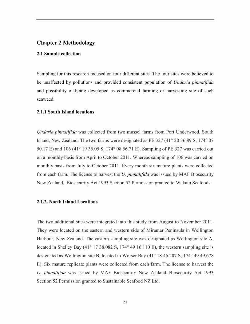
Chapter 2 Methodology .................................................................................................. 21
2.1 Sample collection ................................................................................................... 21
2.1.1 South Island locations ....................................................................................... 21
2.1.2. North Island Locations .................................................................................... 21
2.1.3 Commercial samples ......................................................................................... 24
2.1.4 Seaweed pre-treatment ..................................................................................... 24
2.2 Metals analysis ....................................................................................................... 25
2.2.1 Acid digestion ................................................................................................... 25

III
2.2.2 Advantage of Inductively coupled plasma atomic emission spectroscopy (ICP-
AES). ......................................................................................................................... 27
2.2.3 Chemistry of Inductively coupled plasma atomic emission spectroscopy (ICP-
AES) .......................................................................................................................... 28
2.2.4 Measurement of metals ..................................................................................... 29
2.2.5 Metal element standards ................................................................................... 30
2.2.6 Quality control .................................................................................................. 31
2.3 Pilot studies ............................................................................................................ 32
2.3.1 Comparison of fresh and dried of Undaria pinnatifida digestion .................... 32
2.3.2 Comparison of sample size ............................................................................... 32
2.3.3 Comparison of freeze dried and oven dried samples ........................................ 33
2.4 Statistical analysis ................................................................................................. 33
2.4.1 Statistical analysis for pilot studies .................................................................. 33
2.4.2 Statistical analysis for main study .................................................................... 34
Chapter 3 Results ............................................................................................................ 35
3.1 Pilot studies results ................................................................................................ 35
3.1.1 Comparison of fresh versus dried sample digestion ......................................... 35
3.1.2 Comparison of sample size ............................................................................... 36
3.1.3 Comparison of freeze dried versus oven dried samples ................................... 36
3.2 Spatial and temporal variation of calcium concentrations in Undaria
pinnatifida ..................................................................................................................... 37
3.3 Spatial and temporal variation of potassium concentrations in Undaria
pinnatifida ..................................................................................................................... 41
3.4 Spatial and temporal variation of magnesium concentrations in Undaria
pinnatifida ..................................................................................................................... 44
3.5 Spatial and temporal variation of sodium concentrations in Undaria
pinnatifida ..................................................................................................................... 47
3.6 Spatial and temporal variation of phosphorus concentrations in Undaria
pinnatifida ..................................................................................................................... 50
3.7 Spatial and temporal variation of chromium concentrations in Undaria
pinnatifida ..................................................................................................................... 53
IV
3.8 Spatial and temporal variation of copper concentrations in Undaria pinnatifida
....................................................................................................................................... 56
3.9 Spatial and temporal variation of manganese concentrations in Undaria
pinnatifida ..................................................................................................................... 59
3.10 Spatial and temporal variation of nickel concentrations in Undaria
pinnatifida ..................................................................................................................... 62
3.11 Spatial and temporal variation of selenium concentrations in Undaria
pinnatifida ..................................................................................................................... 65
3.12 Spatial and temporal variation of zinc concentrations in Undaria pinnatifida
....................................................................................................................................... 68
3.13 Spatial and temporal variation of arsenic concentrations in Undaria
pinnatifida ..................................................................................................................... 71
3.14 Spatial and temporal variation of cadmium concentrations in Undaria
pinnatifida ..................................................................................................................... 74
3.15 Spatial and temporal variation of mercury concentrations in Undaria
pinnatifida ..................................................................................................................... 77
3.16 Spatial and temporal variation of lead concentrations in Undaria pinnatifida
....................................................................................................................................... 79
Chapter 4 Discussion ...................................................................................................... 82
4.1 Evaluation of New Zealand Undaria pinnatifida mineral contents ................... 82
4.1.1 Calcium ............................................................................................................. 84
4.1.2 Potassium .......................................................................................................... 84
4.1.3 Sodium .............................................................................................................. 85
4.1.4 Magnesium ....................................................................................................... 87
4.1.5 Phosphorus ........................................................................................................ 88
4.1.6 Chromium ......................................................................................................... 88
4.1.7 Copper .............................................................................................................. 89
4.1.8 Manganese ........................................................................................................ 90
4.1.9 Nickel ................................................................................................................ 90
4.1.10 Selenium ......................................................................................................... 91
4.1.11 Zinc ................................................................................................................. 92

V
4.2 Evaluation of possible heavy metals contaminations in New Zealand Undaria
pinnatifida ..................................................................................................................... 93
4.2.1 Arsenic .............................................................................................................. 93
4.2.2 Cadmium .......................................................................................................... 94
4.2.3 Mercury ............................................................................................................ 94
4.2.4 Lead .................................................................................................................. 95
4.3 Distribution of metals between the blade and sporophyll tissue of Undaria
pinnatifida. .................................................................................................................... 96
4.4 Temporal variation of metals in Undaria pinnatifida ......................................... 96
4.5 Evaluation of Undaria pinnatifida harvesting activities in Port Underwood and
Wellington .................................................................................................................... 97
4.6 Conclusion .............................................................................................................. 99
References ...................................................................................................................... 101
Appendix 1: Statistical outputs for the comparison of sample size .......................... 114
Appendix 2: Statistical outputs for the comparison of freeze dried versus oven dried
samples ........................................................................................................................... 129
Appendix 3: Table of metal contents of Undaria pinnatifida collected from four
different sites in New Zealand. .................................................................................... 133

VI
List of Figures
Figure 1. Alginate monomers. .......................................................................................... 16
Figure 2. Chain sequences of the alginate polymer. ......................................................... 17
Figure 3. Ca binding in alginate associated with the “Egg box” model (Davis et al., 2003).
................................................................................................................................... 18
Figure 4. The location of Port Underwood sampling sites. ............................................. 22
Figure 5. The location of Wellington sampling sites. ....................................................... 23
Figure 6. Varian Liberty ICP AX Sequential Inductively coupled plasma atomic emission
spectroscopy (ICP-AES) ............................................................................................ 25
Figure 7. Acid Digestion on VELP Scientifica DK20 heating digester, the brown fumes
indicated the formation of NO2 as pulverized samples were being digested by HNO3.
................................................................................................................................... 27
Figure 8. Emission of radiation occurred when electron return to the ground state from
excited state. .............................................................................................................. 29
Figure 9. Monthly calcium concentrations in Undaria pinnatifida. ................................. 37
Figure 10. Monthly potassium concentrations in Undaria pinnatifida............................. 41
Figure 11. Monthly magnesium concentrations in Undaria pinnatifida. ......................... 44
Figure 12. Monthly sodium concentrations in Undaria pinnatifida. ................................ 47
Figure 13. Monthly phosphorus concentrations in Undaria pinnatifida. ......................... 50
Figure 14. Monthly chromium concentrations in Undaria pinnatifida. ........................... 53
Figure 15. Monthly copper concentrations in Undaria pinnatifida. ................................. 56
Figure 16. Monthly manganese concentrations in Undaria pinnatifida. .......................... 59
Figure 17. Monthly nickel concentrations in Undaria pinnatifida. .................................. 62

VII
Figure 18 Monthly selenium concentrations in Undaria pinnatifida. .............................. 65
Figure 19. Monthly zinc concentrations in Undaria pinnatifida. ..................................... 68
Figure 20. Monthly arsenic concentrations in Undaria pinnatifida. ................................ 71
Figure 21. Monthly cadmium concentrations in Undaria pinnatifida. ............................. 74
Figure 22. Monthly mercury concentrations in Undaria pinnatifida. .............................. 77
Figure 23. Monthly lead concentrations in Undaria pinnatifida. ..................................... 79
VIII
List of Tables
Table 1.Elements targeted in this thesis .............................................................................. 8
Table 2. Information of commercial product samples ...................................................... 24
Table 3. Results of One-way ANOVA testing for differences in farm PE327 for calcium
concentrations between months for both blade and sporophyll tissue ...................... 38
Table 4. Two way analysis of Variance of calcium in the period between August and
October for blade and sporophyll tissue .................................................................... 39
Table 5. Comparison of the blade and sporophyll tissue content of calcium ................... 40
Table 6. Results of a One-way ANOVA testing for differences in farm PE327 for
potassium concentrations between months in both blade and sporophyll tissue. ...... 42
Table 7. Two way analysis of Variance of potassium in the period between August and
October for blade and sporophyll tissue. ................................................................... 43
Table 8. Comparison of the blade and sporophyll tissue content of potassium ................ 43
Table 9. Results of a One-way ANOVA testing for differences in farm PE327 for
magnesium concentrations between months in both blade and sporophyll tissue..... 45
Table 10. Two way analysis of Variance for magnesium in the period between August
and October for blade and sporophyll tissue. ............................................................ 46
Table 11. Comparison of the blade and sporophyll tissue content of magnesium ........... 46
Table 12. Results of One-way ANOVA testing for differences in farm PE327 for sodium
concentrations between months in both blade and sporophyll tissue ........................ 48
Table 13. Two way analysis of Variance for sodium in the period between August and
October for blade and sporophyll tissue .................................................................... 49
Table 14. Comparison of blade and sporophyll tissue content of sodium ........................ 50
IX
Table 15. Results of a One-way ANOVA testing for differences in farm PE327 for
phosphorus concentrations between months in both blade and sporophyll tissue..... 51
Table 16. Two way analysis of Variance of phosphorus in the period between August and
October for blade and sporophyll tissue. ................................................................... 52
Table 17. Comparison of the blade and sporophyll tissue content of phosphorus ........... 52
Table 18. Results of a One-way ANOVA testing for differences in farm PE327 for
chromium concentrations between months in both blade and sporophyll tissue....... 54
Table 19. Two way analysis of Variance for chromium in the period between August and
October for blade and sporophyll tissue .................................................................... 55
Table 20. Comparison of the blade and sporophyll tissue content of chromium ............. 56
Table 21. Results of a One-way ANOVA testing for differences in farm PE327 for copper
concentrations between months in both blade and sporophyll tissue. ....................... 57
Table 22. Two way analysis of Variance for copper in the period between August and
October for blade and sporophyll tissue. ................................................................... 58
Table 23. Comparison of the blade and sporophyll tissue content of copper ................... 58
Table 24. Results of One-way ANOVA testing for differences in farm PE327 for
manganese concentrations between months in both blade and sporophyll tissue ..... 60
Table 25. Two way analysis of Variance for manganese in the period between August and
October for blade and sporophyll tissue .................................................................... 61
Table 26. Comparison of the blade and sporophyll tissue content of manganese ............ 61
Table 27. Results of One-way ANOVA testing for differences in farm PE327 for nickel
concentrations between months in both blade and sporophyll tissue ........................ 63
Table 28. Two way analysis of Variance of nickel in the period between August and
October for blade and sporophyll tissue .................................................................... 64

X
Table 29. Comparison of the blade and sporophyll tissue content of nickel .................... 64
Table 30. Results of One-way ANOVA testing for differences in farm PE327 for
selenium concentrations between months in both blade and sporophyll tissue......... 66
Table 31. Two way analysis of Variance of selenium in the period between August and
October for blade and sporophyll tissue .................................................................... 67
Table 32 Comparison of the blade and sporophyll tissue content of Selenium ................ 67
Table 33. Results of One-way ANOVA testing for differences in farm PE327 for zinc
concentrations between months in both blade and sporophyll tissue ........................ 69
Table 34. Two way analysis of Variance of zinc in the period between August and
October for blade and sporophyll tissue .................................................................... 70
Table 35. Comparison of the blade and sporophyll tissue content of zinc ....................... 70
Table 36. Results of a One-way ANOVA testing for differences in farm PE327 for
arsenic concentrations between months in both blade and sporophyll tissue ............ 72
Table 37. Two way analysis of Variance of arsenic between sites and time in the period
between August to October for blade and sporophyll tissue ..................................... 72
Table 38. Comparison of the blade and sporophyll tissue content of arsenic ................... 73
Table 39. Results of a One-way ANOVA testing for differences in farm PE327 for
cadmium concentrations between months in both blade and sporophyll tissue ........ 75
Table 40. Two way analysis of Variance of cadmium in the period between August and
October for blade and sporophyll tissue .................................................................... 76
Table 41. Comparison of the blade and sporophyll tissue content of cadmium ............... 76
Table 42. Results of a One-way ANOVA testing for differences in farm PE327 for
mercury concentrations between months in blade tissue. .......................................... 77

XI
Table 43. Two way analysis of Variance for mercury in the period between August and
October for blade tissue. ............................................................................................ 78
Table 44. Results of a One-way ANOVA testing for differences in farm PE327 for lead
concentrations between months in both blade and sporophyll tissue. ....................... 80
Table 45. Two way analysis of Variance of lead in the period between August and
October for blade and sporophyll tissue .................................................................... 80
Table 46. Comparison of the blade and sporophyll tissue content of lead ....................... 81
Table 47. Consumption of 40g of wild Undaria pinnatifida obtained in October 2011.
RDI = recommended daily intake; AI = adequate intake; UI = upper level of intake;
TDI = tolerable daily intake (per 70 kg body weight); TWI = tolerable weekly intake
(per 70 kg body weight). ............................................................................................ 83

XII
Attestation of Authorship
I hereby declare that this submission is my own work and that, to the best of my
knowledge and belief, it contains no materials previously published or written by another
person (except where explicitly defined in the acknowledgments), nor material which to a
substantial extent has been submitted for the award of any other degree or diploma of a
university or other institution of higher learning.
Signed: _______________________________ Date: ________________
Leo Hau

XIII
Acknowledgements
I would like to express my thanks to my supervisor Dr. Lindsey White of Auckland
University of Technology. His guidance and patience had given me strength to complete
my thesis year.
Also I would like to thank Dr. John Robertson useful technical comments and assistance
during the project.
Thanks to Chris Whyburd, Wang Yan, and Percy Perera, for their help with preparing
laboratory equipments, which allowed me to work freely and achieved the best results.
Thanks to Lea and Neil Bramley for their efforts for sampling in the Wellington region
and their enthusiasm for the seaweed industry and my project. Thanks to Mark Allsopp,
and other staff at Wakatu Inc. for arranging the collection trips in Port Underwood. Also
thanks to Weiwei Chen, Glenn Farrington and Savisene Boulom for seaweed collection in
Port Underwood.Last, but not least, I am grateful to my parents, my girl friend and my
friends for their moral support.

XIV
Abstract
Undaria pinnatifida, Wakame is a popular edible seaweed in Asia (Yamanaka &
Akiyama, 1993). Wakame has been recognized as a food rich in minerals, fiber and
bioactive compounds such as proteins, vitamins, carotenoids such as fucoxanthin, and
polyunsaturated fatty acids (Murata & Nakazoe, 2001).
U. pinnatifida was first recorded in New Zealand in Wellington Harbor in 1987. (Hay &
Luckens, 1987) It was classified as an unwanted species according to the Biosecurity Act
1993 under section 164c however, when it was clear that it could not be eradicated a new
policy was applied in April 2010, which allowed greater freedom to use U. pinnatifida
commercially.
The primary aim for this study was to evaluate the concentrations of arsenic (As),
cadmium (Cd), chromium (Cr), copper (Cu), calcium (Ca), mercury (Hg), magnesium
(Mg), manganese (Mn), sodium (Na), nickel (Ni), phosphorus (P), potassium (K), lead
(Pb), selenium (Se) and zinc (Zn) in U. pinnatifida and to compare the metal
concentrations between the blade and sporophyll tissue. These data were compared with
nutrient reference values for Australia and New Zealand and WHO/FAO guidelines to
determine the safety and suitability of harvesting U. pinnatifida to manufacture edible
wakame products.
U. pinnatifida was collected from two mussel farms, PE 327 and 106 from Port
Underwood, South Island, New Zealand. Sampling of PE 327 was carried out on a
monthly basis from April 2011 to October 2011. Sampling of 106 was carried on monthly
basis from July 2011 to October 2011. Two additional sites on the eastern and western
side of Miramar Peninsula in Wellington Harbor; Shelley Bay (site A) and Worser Bay
(site B) were integrated into the study from August 2011 to November 2011.
Harvested samples were dried by oven or freeze dried method then ground to a powder
using a blade mill. The dried U pinnatifida was digested with nitric acid and perchloric

XV
acid and the resulting solutions then analysed by inductively coupled plasma atomic
emission spectroscopy (ICP-AES).
In brief, the highest monthly mean concentration of metals found in New Zealand wild U.
pinnatifida were Ca (16.97 g kg-1
), K (48.48 g kg-1
), Mg (9.47 g kg-1
), Na (62.55 g kg-1
),
P (12.05 g kg-1
), Cr (1.04 mg kg-1
), Cu (3.78 mg kg-1
), Mn (14.61 mg kg-1
), Ni (2.78 mg
kg-1
), Se (0.83 mg kg-1
), Zn (35.03 mg kg-1
), As (46.71 mg kg-1
), Cd (2.91 mg kg-1
), Hg
(0.042 mg kg-1
) and Pb (0.31m g kg-1
).
The results showed that New Zealand U. pinnatifida is a good source of the nutritionally
important minerals calcium, sodium, magnesium, potassium and phosphorus. They also
contained trace amounts of minerals such as chromium, copper, manganese, nickel,
selenium and zinc. Contaminants such as arsenic, cadmium, mercury and lead were
found at very low, safe, levels.

1
Chapter 1 Introduction
There is a lot of interest in the use of seaweeds, either as whole foods or refined for their
active components (McHugh, 2003). These interests have driven academic research
programs and government funded projects, as well as private commercial new product
development initiatives. The majority of these efforts has targeted commonly available
seaweed genera and is focused on whole plants as functional foods, or targets specific
refined compounds with demonstrated bioactivity. Another major global focus has been
the collection of seaweeds from specific regions and then the screening of these seaweeds
for specific bio activity, food safety and their content of various compounds of interest.
Seaweeds have been employed as food and medicines in many Asian countries such as
Japan, Korea, China, Vietnam, Indonesia and Taiwan for a long period of time (McHugh,
2002; Barsanti & Gualtieri, 2006.) . Wakame, U. pinnatifida, is the most popular edible
seaweed in Asia. It has a sweet flavour and is most often served in soups and salads
(Murata & Nakazoe, 2001).
Asian countries, especially Japan and Korea are the main
suppliers and use the most U. pinnatifida and related products and have already
successfully developed cultivation techniques and commercialisation of U. pinnatifida
related products.
Seaweed consumption and usage has existed in New Zealand for a very long period of
time. In the early 1800s, long before the European settlement, the traditional Maori diet
and medicine had often included a number of seaweeds (Brooker, Cambie, & Cooper,
1981). Seaweed such as Ulva spp. Porphyra spp. and Gigartina spp. were often included
(Crowe, 1981). Brown seaweeds such as Durvillaea antarctica (rimuroa), were roasted
and eaten as a curative for eczema and intestinal upsets (Brooker et al., 1981; Crowe,
1981). European immigrants consumed Porphyra spp. as food and made milk puddings
using carrageenan extracted from seaweeds such as Gigartina spp. and more recently
Porphyra spp. was sent to New Zealand troops in World War II as a replacement of
chewing gum (Brooker et al., 1981).

2
1.1 Introduction of Undaria pinnatifida in New Zealand
Undaria pinnatifida was first recorded in New Zealand in Wellington Harbor in 1987
(Hay & Luckens, 1987). The gametophytes were transported to New Zealand in the
ballast of foreign fishing vessels (Neill, Heesch, & Nelson, 2009). At present, U.
pinnatifida in New Zealand has been reported from Great Barrier Island, Auckland
(Waitemata Harbor), Coromandel, Tauranga, Gisborne, Napier, Port Taranaki,
Wellington and the Wellington region of Cook Strait in the North Island, in the
Marlborough Sounds, Nelson, Golden Bay, Kaikoura, Lyttelton, Akaroa, Timaru,
Oamaru, Dunedin Harbor, Bluff in the South Island and also from Stewart Island and the
Snares Islands (Neill et al., 2009). Unlike more tropical climates where there is
significant dieback in warm conditions, U. pinnatifida has displayed an annual life cycle
in New Zealand waters (Neill et al., 2009).
In 2000 U. pinnatifida is classified as an unwanted species according to the Biosecurity
Act 1993 under section 164c (MAF, 2009). However, by 2004 a policy was developed
that allowed the commercial harvest of the seaweed in two situations: where it was taken
as a by-product of another activity, for example, the clearing of mussel farming lines or
as part of a control or eradication programme (MAF, 2009). In 2009 to 2010 the
government had reviewed the 2004 policy related to limited commercialisation of U.
pinnatifida and had revised a new policy in April 2010 allowing greater freedom for the
marine industry to use this seaweed commercially (MAF, 2010).
The new 2010 policy was summerised into four main points (MAF, 2010).
1. The farming of U. pinnatifida is to be allowed in selected infested areas.
2. Harvest of U. pinnatifida can be carried out on artificial surfaces such as marina
and sea farm.
3. Harvest can be carried out in areas not vulnerable or sensitive to commercial
harvest techniques if the U. pinnatifida is casted ashore.
4. Harvest is prohibited from natural surfaces but except when part of a programme
specifically designed to control U. pinnatifida.

3
1.2 Biology of Undaria pinnatifida
The laminarian kelp Undaria pinnatifida (Laminariales, Phaeophyta) has a biphasic life
cycle, the sporophyte (diploid) stage which is macroscopic and is visible to the naked eye
and its gametophyte (haploid) stage which is microscopic in size (Saito, 1975). Although
the durability of its sporophytes stage is approximately six months, the gametophyte stage
is able to remain viable for more than 24 months (Stuart, 2003).
In the sporophyte state colour can vary from yellowish to dark brown and the size can
range up to two metres in length. In its mature state and it can be up to three metres
(Lobban & Harrison, 1996). Mature sporophytes of U. pinnatifida have holdfasts which
act as anchorage for the sporophytes and give rise to the stipe (Lobban & Harrison, 1996).
Hay (1990) further described U. pinnatifida structure as follows, a strap-like midrib (1-3
cm wide), which runs the full length of the thallus with edges of the midrib expanded as a
thin, membranous, pinnatifid blade with pinnae (50-80 cm long).
When U. pinnatifida reaches its mature state, the sporophylls develop on bilateral sides of
the stipe (Hay, 1990; Gibbs & Hay, 1998). Reproduction occurs by the annual release of
asexual zoospores by the mature sporophyll (Parsons, 1994; Oh & Koh, 1996). Millions
of haploid zoospores drift with the seawater until they reach a suitable site for attachment
(Oh & Koh, 1996). Attached zoospores germinate into microscopic male and female
gametophytes (Stuart, 2003). These gametophytes are able to remain viable for up to
three years in their dormant state before they germinate (Ohno & Matsuoka, 1993). Male
gametophytes release mobile sperm into the surrounding water while female
gametophytes produce eggs which remain on the gametophyte (Saito, 1975). Mobile
sperm fertilises the egg, which begins to form a germling which develops into new
sporophytes (Saito, 1975).
U. pinnatifida is an annual seaweed (Saito, 1975; Hay, 1990) . In late summer and early
autumn mature seaweeds degenerate and new sporophyte become established (Hay &

4
Villouta, 1993). In Japan, sporophytes of U. pinnatifida are completely dieback during
autumn when water temperatures drop below 20°C (Saito, 1975; Ohno & Matsuoka,
1993). However some New Zealand populations, for example in the Wellington harbour,
exhibit overlapping generations and sporophytes can be found year-round. (Hay &
Villouta, 1993). This phenomenon might be attributed to the narrower range of annual sea
temperature of the New Zealand water when compared to those in Japan and Korean
(Hay & Villouta, 1993).

5
1.3 Economic values and applications of seaweed
The aquaculture industry produced 15.8 million tonnes of aquatic plants in 2008, which
has an estimated value of US$ 7.4 billion. The industry has enjoyed a consistent
production growth rate of 7.7% annually (FAO, 2010). The production of aquatic plants
was dominated by the production of seaweeds, 99.6 % by quantity and 99.3 % by value in
2008 (FAO, 2010).
East and Southeast Asian countries dominate seaweed culture, 99.8 % by quantity and
99.5 % by value in 2008, with almost all the seaweed species in these areas cultured for
human consumption. (FAO, 2010). In 2008, China produced 62.8% of the world’s
aquaculture production of seaweeds by quantity followed by Indonesia (13.7 %), the
Philippines (10.6 %), the Republic of Korea (5.9 %), Japan (2.9 %) and the Democratic
People’s Republic of Korea (2.8 %) (FAO, 2010). However Japan is the second-most
important aquatic plant producing country in terms of value (US$ 1.1 billion), because of
to its high-priced Nori production (FAO, 2008, 2010). Other use of seaweed include
Eucheuma seaweed which is used as the major species for carrageenan extraction and
Japanese kelp which is used as a raw material for the extraction of iodine and alginate
(Barsanti & Gualtieri, 2006.). Chile was the most important seaweed culturing country
outside Asia, producing 21,700 tonnes in 2008 while 14,700 tonnes produced in Africa
(FAO, 2010).
The highest production of cultured seaweed in 2008 was of Japanese kelp (Laminaria
japonica, 4.8 million tonnes), followed by Eucheuma seaweeds (Kappaphycus alvarezii
and Eucheuma spp., 3.8 million tonnes), Wakame (Undaria pinnatifida, 1.8 million
tonnes), Gracilaria spp. (1.4 million tonnes) and Nori (Porphyra spp., 1.4 million tonnes)
(FAO, 2010).

6
1.4 Economic values and application of Undaria pinnatifida
U. pinnatifida has been cultured and collected from natural habitats for centuries. It is one
of the main commercially harvested and cultivated species in Asia, and its range has been
extended by intentional introductions and translocations for aquaculture from China and
to Atlantic France and Mediterranean France however most movement of U. pinnatifida
has been by unintentional introductions to Europe, USA, Australia, New Zealand, Mexico
and Argentina (McHugh, 2003).
Wakame is more popular in the Republic of Korea than in Japan, although the market in
Japan had expanded (McHugh, 2003). The current harvest is between 450,000 and
500,000 tonnes in Japan and Korea respectively with China producing a few hundred
tonnes (FAO, 2012a). The global production harvest of wild U. pinnatifida was 4783
tonnes in 2010 (FAO, 2012b).
Wakame has high total dietary fiber content, higher than Nori or Kombu. Like the other
brown seaweeds, the fat content of Wakame is quite low. Air-dried Wakame has similar
vitamin content to the wet seaweed and is relatively rich in the vitamin B group,
especially niacin (McHugh, 2003; Kolb, Vallorani, Milanovic, & Stocchi, 2004) . Raw
Wakame contains substantial amounts of essential trace elements such as manganese,
copper, cobalt, iron, nickel and zinc, similar to Kombu and Hijiki (McHugh, 2003).
Processed Wakame is a very convenient form, used for various instant foods such as
noodles and soups (Murata & Nakazoe, 2001; McHugh, 2003). The most common dried
Wakame product is made from blanched and salted Wakame which is washed with
freshwater to remove salt, cut into small pieces, dried in a flow-through dryer and passed
through sieves to sort the different sized pieces (Watanabe & Nısizawa, 1984; McHugh,
2003). It has a long storage life and has a fresh green colour when rehydrated (Murata &
Nakazoe, 2001; McHugh, 2003).
In addition to human consumption as a regular food item, there is growing interest of U.
pinnatifida in the health food and pharmaceutical markets (Hwang, Gong, & Park, 2011).

7
U. pinnatifida has also proved to be an very useful source of Fucoidan, a fucose-
containing sulfated poly-saccharide found in brown algae and proven to have
anticoagulant and antiviral activities (Noda, Amano, Arashima, & Nisizawa, 1990; Lee,
Hayashi, Hashimoto, & Nakano, 2004). Antioxidant compounds such as Fucoxanthin,
have been extracted from U. pinnatifida (Yan, Chuda, Suzuki, & Nagata, 1999).
Antiviral activities from U. pinnatifida had also been confirmed to inhibit the Herpes
simplex virus (Khan & Satam, 2003).
The commercial value of U. pinnatifida varies according to the quality, origin of the
product and end use (MAF, 2009). Aquaculture New Zealand estimated that U.
pinnatifida could return between NZ$ 500/tonne as bulk seaweed for use in agricultural
products (Aquaculture New Zealand, 2008). Estimates of more than NZ$ 1000/tonne for
premium grade food U. pinnatifida uses has also been suggested (Aquaculture New
Zealand, 2008). Aquaculture New Zealand estimated that in the Marlborough Sounds
there is, on average, 5 tonnes of wild U. pinnatifida per long-line and note that there are
thousands of long-lines in the Marlborough Sounds (Aquaculture New Zealand, 2008).

8
1.6 Metals in Undaria pinnatifida
Given that Undaria pinnatifida is regularly consumed by large number of humans and U.
pinnatifida is now able to be harvested as a commercial product in New Zealand, it is
important to examine the nutritional quality of New Zealand U. pinnatifida. This thesis
focuses on metals components in U. pinnatifida as these metals have been shown to have
impact on human health (Hunter, Simpson, & Strank, 1980; Almela et al., 2002; Rupérez,
2002; Almela, Jesus Clemente, Velez, & Montoro, 2006; MacArtain, Gill, Brooks,
Campbell, & Rowland, 2007; Rose et al., 2007; Besada, Andrade, Schultze, & González,
2009; Hwang, Park, Park, Choi, & Kim, 2010; Smith, Summers, & Wong, 2010). Fifteen
metals were chosen in this study
Table 1.Elements targeted in this thesis
Heavy Metals Chemical symbols
Arsenic As
Cadmium Cd
Mercury Hg
Lead Pb
Minerals
Calcium Ca
Potassium K
Magnesium Mg
Sodium Na
Phosphorus P
Chromium Cr
Copper Cu
Manganese Mn
Nickel Ni
Selenium Se
Zinc Zn

9
1.7 Effect of metals on human health
Heavy metals are members of a loosely-defined subset of elements that exhibit metallic
properties, which include the transition metals, some metalloids, lanthanides, and
actinides (Hunter et al., 1980).
Common metals are all naturally occurring substances that are often present in the
environment at low levels. They can be dangerous to humans if they are exposed in large
amounts to these metals by ingestion (drinking or eating) or inhalation (Singh, Gautam,
Mishra, & Gupta, 2011). Heavy metals become toxic when they are not metabolised by
the body and accumulate in the tissues and organs. Various food poisoning cases, due to
heavy metal contamination of the coastal environment had been reported internationally
(Phillips & Rainbow, 1992). Different heavy metals have different effects on human
health. For example, elements such as cadmium, lead and mercury are more harmful than
the other metal compounds (Manahan, 1993). Mercury poisoning was reported in
Minimata Bay Japan, in the eastern Shiranui sea in 1953, where fish and shellfish were
contaminated with mercury (Phillips & Rainbow, 1992). Mercury poisoning due to
aquatic contamination had also been reported from several other parts of the world,
including Sweden, Canada and the USA (Phillips & Rainbow, 1992).
Calcium is an important mineral for human bone development (Heaney, 1986;
Anonymous, 2005). It plays a minor role in the body, such as some exocytosis,
neurotransmitter release, and muscle contraction (Heaney, Saville, & Recker, 1975;
WHO, 2004). Compared with other metals, calcium and most calcium compounds have
low toxicity. This is expected as it has very high natural abundance in the environment
and in organisms (WHO, 2004). Calcium poses few serious environmental problems and
acute calcium poisoning is rare, and difficult to achieve unless calcium compounds are
administered intravenously (WHO, 2004).
Potassium ions are important in neuron function and in influencing osmotic balance
between cells and the interstitial fluid (Whelton et al., 1997; Anonymous, 2005; WHO,

10
2009). This element also controls muscle contraction and the sending of all nerve
impulses through action potentials (Whelton et al., 1997; Anonymous, 2005; WHO,
2009). The primary source of K for the general population is the diet, as K is found in all
foods, particularly vegetables and fruits (Holbrook et al., 1984). Potassium intoxication
by ingestion is rare, because high level potassium is rapidly excreted in healthy kidney
and caused vomiting (Wetli & Davis, 1978; Holbrook et al., 1984; WHO, 2009).
Magnesium is essential to all cells of all known living organisms. Mg is used as a
cofactor of many enzymes involved in energy metabolism, protein synthesis, RNA and
DNA synthesis, and maintenance of the electrical potential of nervous tissues and cell
membranes (Schroeder, Nason, & Tipton, 1969; Al-Ghamdi, Cameron, & Suton, 1994).
It is important to monitor magnesium levels carefully as this element regulates potassium
fluxes and its involvement in the metabolism of calcium in humans (Classen, 1984; WHO,
2004). Over dose of Mg is rare, as excess magnesium in the body can be cleared by
healthy kidneys easily (Quarme & Disks, 1986).
Sodium is an essential nutrient that regulates blood volume, blood pressure, osmotic
equilibrium and pH. Sodium is the primary electrolyte which regulates the extracellular
fluid levels in the body (Fregly, 1984). Na is essential for hydration because this mineral
pumps water into the cell (Fregly, 1984). Excessive consumption of Na on a regular basis
is often associated with hypertension and edema, further high intakes of sodium could
lead to osteoporosis because sodium may increase urinary lost of calcium (Fuchs et al.,
1987).
The main sources of phosphorus for humans are foods containing protein (Nordin, 1989).
Inorganic phosphorus in the form of the phosphate PO43–
is required for all known forms
of life playing a major role in molecules such as DNA and RNA where it is involved in
structural construction. Living cells also use P to transport cellular energy in the form of
adenosine triphosphate (ATP) (Nordin, 1989). Deficiency of P can lead to symptoms of
hypophosphatemia, muscle and neurological dysfunction, and disruption of muscle and
blood cells due to lack of ATP (Lotz, Zisnman, & Bartter, 1968; Nordin, 1989). Too

11
much P could lead to diarrhoea, calcification of organs and soft tissue, and could interfere
with the body's ability to use element such as calcium (Spencer, Menczel, Lewin, &
Samachson, 1965).
Chromium is often found in rocks, animals, plants, and soil and could be a liquid, solid,
or gas. Chromium (VI) compounds are toxins and known human carcinogens, whereas
Chromium (III) is an essential nutrient at moderate level (Lim, Sargent, & Kusubov, 1983;
Das, Grewal, & Banerjee, 2011). Breathing high levels of Cr can cause irritation to the
lining of the nose and breathing problems, such as asthma (Das et al., 2011). High
chromium intakes may cause renal failure, genotoxicity, and are carcinogenic to human
(Stearns, Wise, Patierno, & Wetterhahn, 1995; Loubieres et al., 1999).
Copper in the environment occurs mainly though electroplating industries and sewage
effluents (Hickey, 1992; Donohue, 2004). Copper is also a component of a number of
metalloenzymes including diamine oxidase and monoamine oxidase (Turnlund, 1998).
Copper is widely distributed in foods with organ meats, seafood, nuts and seeds being
major contributors (Harris, 1997). Long term exposures of Cu cause cirrhosis of the liver
and jaundice (Harris & Gitlin, 1996). Whereas deficiency of Cu in the body could cause
symptoms such as weight loss, bone disorders and microcytic hypochromic anaemia
(Higuchi, Higashi, Nakamura, & Matsuda, 1988; Singh et al., 2011).
Manganese is used principally in the manufacture of iron and steel alloys (Du, 2011).
Compounds containing manganese have also been used as an ingredient in various
products such as batteries, glass, fertilizers and livestock feeding supplements (Du, 2011).
Mn is an essential element for many living organisms, including humans. For example,
some enzymes require manganese e.g. manganese superoxide dismutase, and some are
activated by the element e.g. kinases, decarboxylases (Finley, Johnson, & Johnson, 1994;
Williams-Johnson, 1999). Inadequate intake or overexposure of Mn could lead to
neurological impairment (Greger, 1998; Du, 2011; Singh et al., 2011). Manganese
deficiency in humans appears to be rare, because many common foods have sufficient
amount of Mn (Du, 2011).

12
Nickel is used mainly in the production of stainless steels, non-ferrous alloys, and super
alloys (Fawell, 2005). Other uses of Ni and Ni salts include electroplating and as catalysts.
Acute absorption of Nickel can cause effects on kidney function, including tubular and
glomerular lesions and it is also a possible carcinogen (Sunderman Jr, Dingle, Hopfer, &
Swift, 1988; Fawell, 2005).
Selenium is a trace mineral widely distributed in most rocks and soils (Das et al., 2011).
Overdose of Se leads to selenosis (Helzlsouer, Jacobs, & Morris, 1985; Das et al., 2011).
Deficiency of Se leads to Keshan Disease (Keshan Disease Research Group, 1979). In
humans, selenium is a trace element nutrient that functions as cofactor for reduction of
antioxidant enzymes, such as glutathione peroxidase and thioredoxin reductase which
involves in controlling tissue concentrations of highly reactive oxygen-containing
metabolites (Whanger, 1998; Holben & Smith, 1999; WHO, 2004). These metabolites are
essential at low concentrations for maintaining cell-mediated immunity against infections
but highly toxic if produced in excess (Whanger, 1998; WHO, 2004).
Zinc is an essential component to over three hundred enzymes participating in the
synthesis and degradation of carbohydrates, lipids, proteins, and nucleic acids as well as
in the metabolism of other micronutrients (King & Keen, 1999). Zn also stabilises the
molecular structure of cellular components and membranes, and as a result integrity of
cells and organs is achieved (King & Keen, 1999; Das et al., 2011). However over
absorption of Zn could cause damage in the nervous system (WHO, 2004; Das et al.,
2011).
Arsenic can be released in large quantities through volcanic activity, erosion of rocks,
forest fires and human activity. Arsenic is odorless and tasteless (Das et al., 2011).
Inorganic arsenic is a known carcinogen and could cause cancer of the skin, lungs, liver
and bladder (Rose et al., 2007). Very high levels can possibly result in death (Das et al.,
2011). Long-term low level exposure can cause a darkening of the skin (Das et al., 2011) .

13
Cadmium is a very toxic metal, which can be found in all soils and rocks, welding,
electroplating, fertilizers and pesticides (Singh et al., 2011). Cadmium and cadmium
compounds are known human carcinogens (Das et al., 2011; Singh et al., 2011).
Ingesting very high levels severely irritate the stomach, leading to vomiting and diarrhea.
Long-term exposure of Cd leads to possible kidney disease, lung damage, increase of
blood pressure and Ca in bone could also be replaced by cadmium causing brittleness of
the bones (Abbe & Riedel, 2000; Das et al., 2011; Singh et al., 2011).
Mercury combines with other elements to form organic and inorganic mercury
compounds. The United States Environmental Protection Agency (EPA) have determined
that mercuric chloride and methyl mercury are possible human carcinogens (Das et al.,
2011). Human exposure to high levels of mercury could permanently damage the brain,
kidneys, developing fetuses and nervous system (Das et al., 2011). Effects on brain
functioning may result in irritability, shyness, tremors, changes in vision or hearing, and
memory problems (Das et al., 2011; Singh et al., 2011).
Lead is a probable human carcinogen (Das et al., 2011). Which can affect every organ
and system in the body (Singh et al., 2011). Exposure to high lead levels could severely
damage the brain, kidneys and cause miscarriage in pregnant women (Das et al., 2011).

14
1.8 Heavy metals in the marine environment
Pollutants in the aquatic environment that are not degraded by biological or chemical
processes have the ability to accumulate in high concentrations in water and sediments of
aquatic habitats (Clark, 1997). Heavy metals are non-degradable pollutants in the aquatic
environment and occur both in sediments and water (Clark, 1997).
Natural processes such as gaseous state and aerosols might cause some heavy metals to
enter the marine environment (Kennish, 1992). It is also possible metals may reach the
sea surface by dry deposition, precipitation, or by gaseous exchange (Kennish, 1997).
Hydrothermal activity in deep seawater is another natural source of heavy metals,
particularly arsenic and mercury (Kennish, 1992). Heavy metals are normally supplied to
the sea by river water or as windborne materials following the weathering of soil in
coastal areas (Penny, 1984). Heavy metals could also be transported by river waters
sewage and water ways systems to coastal environments followed by accumulation in
high concentrations in oceanic environments, where they are presented in particulate and
dissolved forms (Kennish, 1997). Rainwater that contacts impervious surfaces such as
roofs, roads, and concrete surfaces is referred to as stormwater and acts as a major
nonpoint source of heavy metals in estuarine and coastal water (Patin, 1982). Different
contaminants or heavy metals from inland areas can be transported directly or indirectly
to coastal waters in stormwater.
Coastal pollution poses a potential health risk for humans because people all over the
world use coastal organisms as food sources and coastal water for various recreational
purposes (Edwards & Edyvane, 2001). However, the most noticeable health risk is
associated with consumption of seafood in which organic and inorganic pollutants are
often accumulated in the seaweed tissues and marine organisms. (Han & Jeng, 1998).

15
1.9 Metals in brown seaweed -metal accumulation pathways
Accumulation of metals in seaweeds depends on two main factors, the bioavailability of
metals in the surrounding water and the uptake capability of metal by the seaweed (Davis,
Volesky, & Mucci, 2003). Cell walls in seaweeds contain polysaccharides and proteins,
which play an important role in metal retention. The uptake of metals can occur in two
ways. The first is passive uptake, a surface reaction, which metals are absorbed by algal
surfaces through electrostatic attraction to negatives sites (Ishak & Hamzah, 2010). This
is independent on factors which influence the metabolism such as temperature, light, pH
or age of the plant, but it is also influenced by the relative abundance of elements in the
surrounding water (Besada et al., 2009). With passive uptake metal ions adsorb onto the
cell surface within a relatively short span of time, normally within few seconds or
minutes (Besada et al., 2009; Ishak & Hamzah, 2010). The second way metals can be
taken up into seaweeds is a slower active uptake in which metal ions are transported
across the cell membrane into the cytoplasm. This form of uptake is more dependent
upon metabolic processes (Mehta & Gaur, 2005; Ishak & Hamzah, 2010).
The cellular biology of brown seaweeds plays an important role in the metal
accumulation pathway. More specifically, it is the properties of cell wall constituents,
such as alginate and fucoidan, which are solely responsible for metal binding and
accumulations (Davis et al., 2003). Lobban & Harrison (1996) described the structure of
alga cell walls in the following manner; the brown algae cell wall is constructed by at
least two different layers. The inner layer consists of a microfibrillar skeleton which
contributes to the rigidity of the wall. The outer layer is an amorphous embedding matrix.
The amorphous matrix is attached to the microfibrillar skeleton layer by hydrogen bonds
and does not penetrate the fibers. The inner, rigid fibrillar layer of brown algae is mainly
comprised of the uncharged cellulose polymer with β(1-4)-linked unbranched glucan..
The biosorption mechanism of metals is very closely related to the chemistry of the
components of the cell wall. The cell wall properties such as electrostatic attraction and

16
complexation could also influence the absorption of metals. The Brown algal embedding
matrix contains predominately alginic acid or alginate, the salt of alginic acid with a
smaller amount of sulfated polysaccharide (Fucoidan) (Graham & Wilcox, 2000). Alginic
acid or alginate, is the common name given to a family of linear polysaccharides
containing 1,4-linked β-D-mannuronic (M residue) or α-L- guluronic acid (G residue)
residues arranged by covalent bond linked together in different unregular sequences or
blocks (Lobban & Harrison, 1996; Graham & Wilcox, 2000). The monomers appears as
homopolymeric blocks of consecutive G-residues (G-blocks), consecutive M-residues
(M-blocks) or alternating M and G-residues (MG-blocks) (Haug, Larsen, & Smidsrod,
1966). The carboylic acid dissociation constants of M and G had been determined as pKa
= 3.38 and pKa = 3.65; respectively, with similar pKa values for the polymers(Haug,
1961). The main function of alginate is to maintain the strength and flexibility of the cell
wall in brown algae. Alginates made up to around 20%-40% of the dry weight of brown
seaweed (Lobban & Harrison, 1996; Graham & Wilcox, 2000).
Figure 1. Alginate monomers.
M- and G-block sequences have shown significant structural differences and their
proportions in the alginate and contribute to the physical properties and reactivity of the
polysaccharide (Figure 3) (Haug, Myklestad, Larsen, & Smidsrod, 1967).
Polymannuronic acid has flat ribbon-like chain with molecular repeat of 10.35 Å (Atkins,
Mackie, Nieduszynski, Parker, & Smolko, 1973a). It is constructed with two

17
diequatorially (1e-4e) linked β-D-mannuronic acid residues in the chair conformation
(Figure 4) (Atkins et al., 1973a; Graham & Wilcox, 2000) . Whereas, polyguluronic acid
contains two diaxially (1a-4a) linked α-L-guluronic acid residues in the chair conformer
which creates a rod-like polymer with a molecular repeat of 8.7 Å (Figure 4) (Atkins,
Mackie, Nieduszynski, Parker, & Smolko, 1973b; Graham & Wilcox, 2000). This key
difference in molecular conformation between the two homopolymeric blocks is believed
to be chiefly responsible for the variable affinity of alginates for metals. The polymer
conformations of the two different blocks in alginate are different. But this difference
also depends on the genus of the algae and from which part of the plant it comes from
(Davis et al., 2003).
OO O
O
O
O
O
-OOC
OH
OH -OOC
OH
OH
-OOC OH
HO HO
-OOC OH
-OOC
OH
OH
O
O
G G M M G
Figure 2. Chain sequences of the alginate polymer.
The variation of the M: G block ratio is depended on species and possible geographical
factors, which have not been studied in detail (Graham & Wilcox, 2000). Variation in the
affinity of some divalent metals to alginates with different M: G ratios have been
demonstrated (Haug, 1961). Haug (1961) showed that the affinity of alginates for
divalent cations such as Pb2+
, Cu2+
, Cd2+
, Zn2+
, Ca2+
, etc. increased with the guluronic
acid content.
The alginates have an ordered network and adapt an inter-chain dimerization of the
polyguluronic sequences in the presence of calcium or other divalent cations of similar
size (Lobban & Harrison, 1996). The poly-L-guluronic sections have rod like shapes and
alignment of two chains create an array of coordination sites (Lobban & Harrison, 1996;
Davis et al., 2003). These cavities are suitable for divalent cations for example Ca2+
.

18
These divalent ions are bound with the carboxylate oxygen and other oxygen atoms of G
residues, described as the ‘‘egg-box’’ model (Figure 5) (Lobban & Harrison, 1996;
Graham & Wilcox, 2000; Davis et al., 2003). In the end the region of dimerization are
terminated by chain sequences of polymannuronic acid residues (Davis et al., 2003). As a
result, several different chains become interconnected and this contributes to the gel
network formation (Davis et al., 2003).
Figure 3. Ca binding in alginate associated with the “Egg box” model (Davis et al., 2003).
Brown algae also contain 5 to 20% sulfated polysaccharide fucoidan, about 40% of which
is sulfate esters (Davis et al., 2003). Fucoidan can be found in the matrix but also within
the inner cell wall (Davis et al., 2003). Fucoidan is a branched polysaccharide sulfate
ester with L-fucose building blocks, which are predominantly α(1→2) linked. Trivalent
cations mainly bind to sulfated polysaccharides in low pH environments (Davis et al.,
2003).
The algal cell wall also has many functional groups, such as, hydroxyl (OH), phosphoryl
(PO3O2), amino (NH2), and sulphydryl (SH), etc. These functional groups can be found in
various cell wall components, e.g., peptidoglycan, teichouronic acid, teichoic acids,
polysaccharides and proteins (Davis et al., 2003; Mehta & Gaur, 2005). They have the
ability to confer a negative charge to the cell surface. In general, metal ions in water are
in the form of cations and could be easily absorbed onto the call surface (Graham &
Wilcox, 2000; Davis et al., 2003). Each functional group has specific pKa (dissociation

19
constant), and it dissociates into particular anions and protons at a specific pH conditions
(Davis et al., 2003).
It is noteworthy that the distribution and abundance of cell wall components vary among
different algal groups, as to the number and kinds of functional groups (Lobban &
Harrison, 1996). Among different cell wall components, polysaccharides and proteins
have most of the metal binding sites (Lobban & Harrison, 1996). When metals are inside
the cell, they may bind to cytoplasmic ligands, phytochelatins and metallothioneins, and
other intracellular molecules or precipitate (Davis et al., 2003). Metal concentration can
play a role in controlling biological macromolecules and enzymes as they contain
appropriate functional groups or metal co-factors to achieve particular activity (Lobban &
Harrison, 1996).
Brown seaweeds cellular structure in relation in metal binding has been studied and
resulted in more economic benefits. Biosorption is a term that describes the removal of
heavy metals by the passive binding to nonliving biomass from aqueous solution (Mehta
& Gaur, 2005; Wang & Chen, 2009 ; Ishak & Hamzah, 2010). Various seaweeds and
especially brown algae have been used as a raw material to produce biosorbents for the
removal of heavy metals in contaminated areas. For example U. pinnatifida and
Sargassum sp were also proved to be a excellent raw seaweed to be used as biosorbent
for heavy metals (Kim, Yoo, & Lee, 1995; Bina, Kermani, Movahedian, & Khazaei,
2006). More recently Kim et al (1999) demonstrated that the further introduction of
sulphur groups onto the cell surface of U pinnatifida increased the bio-sorption capacity
of lead ions. The total sulphur content of the cell increased to 13.8% (w:w) through
xanthation (Kim, Park, Yoo, & Kwak, 1999). Xanthate groups introduced onto the cell
wall of U pinnatifida enabled the biomass to adsorb lead ions (Kim et al., 1999).

20
1.10 Study aims
The main aim of this study was to evaluate the concentration of metals (Table 1) in
samples of Undaria pinnatifida from New Zealand’s South Island, (Port Underwood) and
North Island, (Wellington) to determine the overall suitability to use Undaria pinnatifida
to manufacture food products in terms of heavy metal safety. The study also aimed to
compare the concentration of metals between the blade and sporophyll tissue and to
investigate the possible seasonal variations of metals in the two locations.
21
Chapter 2 Methodology
2.1 Sample collection
Sampling for this research focused on four different sites. The four sites were believed to
be unaffected by pollutions and provided consistent population of Undaria pinnatifida
and possibility of being developed as commercial farming or harvesting site of such
seaweed.
2.1.1 South Island locations
Undaria pinnatifida was collected from two mussel farms from Port Underwood, South
Island, New Zealand. The two farms were designated as PE 327 (41° 20 36.89 S, 174° 07
50.17 E) and 106 (41° 19 35.05 S, 174° 08 56.71 E). Sampling of PE 327 was carried out
on a monthly basis from April to October 2011. Whereas sampling of 106 was carried on
monthly basis from July to October 2011. Every month six mature plants were collected
from each farm. The license to harvest the U. pinnatifida was issued by MAF Biosecurity
New Zealand, Biosecurity Act 1993 Section 52 Permission granted to Wakatu Seafoods.
2.1.2. North Island Locations
The two additional sites were integrated into this study from August to November 2011.
They were located on the eastern and western side of Miramar Peninsula in Wellington
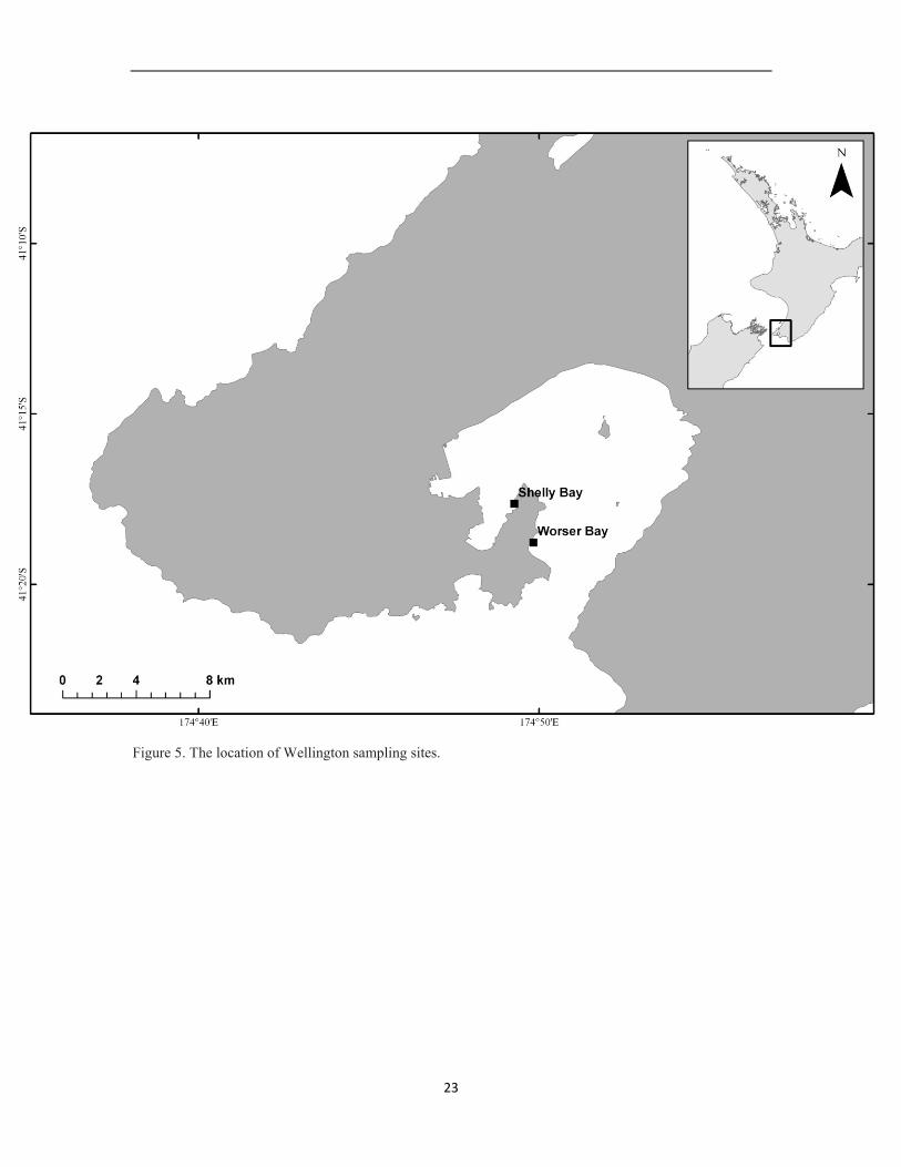
Harbour, New Zealand. The eastern sampling site was designated as Wellington site A,
located in Shelley Bay (41° 17 38.082 S, 174° 49 16.110 E), the western sampling site is
designated as Wellington site B, located in Worser Bay (41° 18 46.207 S, 174° 49 49.678
E). Six mature replicate plants were collected from each farm. The license to harvest the
U. pinnatifida was issued by MAF Biosecurity New Zealand Biosecurity Act 1993
Section 52 Permission granted to Sustainable Seafood NZ Ltd.

22
Figure 4. The location of Port Underwood sampling sites.
23
Figure 5. The location of Wellington sampling sites.

24
2.1.3 Commercial samples
Three bags of three different imported commercial Wakame products were purchased
from a supermarket.
Table 2. Information of commercial product samples
Product name Manufacturer Package weight Origins of
seaweed, claimed
by the label.
Katto Wakame Daichu Shokuhin
Ltd
22g Japan
Fue Fue Wakame
Gureeto
Daichu Shokuhin
Ltd
18g China
Maejima Tabetaro
Cut Wakeme Maejima
Shokuhin Co. Ltd
30g Korea
2.1.4 Seaweed pre-treatment
The seaweed samples collected from PE 327 and 106 were first rinsed with seawater to
remove debris and epiphytic organisms from the thallus. The blade was separated from
the sporophyll and both placed in separate zip-lock bags in a chilli-bin. They were
frozen and flown to the Vitaco Health New Zealand Limited freeze drying plant located
in Blockhouse Bay, Auckland, New Zealand. The samples were freeze dried at -18°C to
remove all moisture. The samples were then shipped to AUT laboratory, grounded to
fine powder by blender and stored in clean polyethyene bottles to await analysis.
The U. pinnatifida samples obtained from Wellington harbor were rinsed with fresh water
to remove debris and epiphytic organisms from the thallus. The blades were separated
from the sporophylls and both placed in separate zip-lock bags and packed in a box and
flown to the laboratory at Auckland University of Technology, Auckland, New Zealand.
The samples were then briefly washed again with de-ionized water to remove possible

25
remaining debris. The samples were dried to constant weight at 60°C in a Sanyo MOV-
112 laboratory oven. They were then ground to fine powder by blender and stored in
clean polystyrene bottles to await analysis.
2.2 Metals analysis
The concentrations of metals in the U. pinnatifida samples were determined by a
modified method of Denton & Burdon-Jones (1986) and Qari & Siddiqui (2010). Briefly,
the dried, ground samples were digested in acid, filtered, diluted and measured on an
inductively coupled plasma atomic emission spectroscopy (ICP-AES) machine (Figure 6).
Figure 6. Varian Liberty ICP AX Sequential Inductively coupled plasma atomic emission spectroscopy
(ICP-AES)
2.2.1 Acid digestion
Acid digestion has been widely used in elemental analysis in many organic samples such
as plant, food, and animal tissues. Acid digestion can be described as mechanical sample
preparation to completely transfer the analytes into solution so they can be introduced
into the determination step, e.g. Inductively coupled plasma atomic emission
spectroscopy (ICP-AES), Inductively coupled plasma mass spectrometry (ICP-MS) or

26
Atomic absorption spectroscopy (AAS) (Worsfold, Townshend, & Poole, 2005). The
goal of every digestion process is therefore the complete solution of the analytes and the
complete decomposition of the solid or matrix while avoiding loss or contamination of
the analyte (Worsfold et al., 2005).
Microwave assisted digestion with a Teflon reactor and nitric acid (HNO3) are the most
common method used in metal analysis of seaweeds (Villares, Puente, & Carballeira,
2001; Mohamed & Khaled, 2005; Al-Shwaf & Rushdi, 2008; Cofrades et al., 2010;
Domínguez-González et al., 2010; Hwang et al., 2010). These methods speed up and
achieve the digestion more effectively (Balcerzak, 2002 ). The drawbacks of this method
are the slow cool down time needed and relatively high operational cost.
Acid digestion using HNO3 followed by additional perchloric acid (HClO4) has been used
in metal analysis (McQuaker, Brown, & Kluckner, 1979; Shaibur, Shamim, Huq, &
Kawai, 2010). Including metal analysis of seaweeds (Denton & Burdon-Jones, 1986 ;
Qari & Siddiqui, 2010). HClO4 prevents excessive frothing which occurs when HNO3
alone was used (Shaibur et al., 2010). It also acts as a helper to complete the digestion of
the materials (Namieśnik, Chrzanowski, & Szpinek, 2003).
As reviewed above, recent research related to metal concentrations in seaweed applied
pressurize and microwave assisted acid digestion methods involving Nitric Acid. This
method, in conjunction with ICP AES was reported as early as 1979 (McQuaker., et al).
Therefore, for both financial and technical reasons acid digestion with HNO3 and HClO4
was chosen as the digestion method in this study.
Acid digestions were carried out by adding an 0.5 g of sample to 10 mL of concentrated
Laboratory Analytical Grade 70% HNO3 in acid digestion block (VELP Scientifica DK20
heating digester – Figure 7). The reaction mixture was heated at 90 °C for 30 minutes and
then 110°C for 2 hours. 5 mL of 80% HClO4 was then added and heating discontinued
when dense white fumes appeared. After cooling, the mixture was filtered through

27
Whatman number 42 filter paper. The resulting solution was finally made up to 50 mL
with deionized water in a volumetric flask.
Figure 7. Acid Digestion on VELP Scientifica DK20 heating digester, the brown fumes indicated the
formation of NO2 as pulverized samples were being digested by HNO3.
2.2.2 Advantage of Inductively coupled plasma atomic emission spectroscopy (ICP-
AES).
An ICP-AES was chosen for the determination of metals as ICP-AES is capable of
analysing multiple elements simultaneously and is more sensitive to some elements than
atomic absorption spectroscopy (AAS). ICP-AES is able to handle both simple and
complex sample matrices with high productivity. ICP-AES has the ability to detect most
of the elements in the periodic table, which makes it an ideal tool in metal detections.
There are four major advantages of ICP AES over AAS.
1. ICP AES has a wide working range, usually from 0.1 to 1000 µg mL-1
. Whereas

28
AAS is ranged from 1 to 10 µg mL-1
(Mendham, Denney, Barnes, & Thomas,
2000).
2. ICP AES is able to perform simultaneous multi element analyses and rapid
sequential analyses (Mendham et al., 2000).
3. ICP AES has precision over AAS by using an internal standard, usually 0.1-1%
relative standard deviation (RSD). With flame AAS the precision is usually 1-2%
RSD and with furnace AAS it is 1-3% RSD (Mendham et al., 2000).
4. Quick measurement of samples can be achieved with ablation and other
vaporization methods (Mendham et al., 2000).
2.2.3 Chemistry of Inductively coupled plasma atomic emission spectroscopy (ICP-
AES)
The Inductively coupled plasma atomic emission spectroscopy (ICP-AES) consists of
two main parts, the ICP and the optical spectrometer. The ICP torch consists of 3
concentric quartz glass tubes (Manning & Grow, 1997). The coil of the radio frequency
(RF) generator surrounds part of this quartz torch. When the torch is in operation, an
intense electromagnetic field is created within the coil by the high power radio frequency
signal flowing in the coil (Manning & Grow, 1997). This RF signal is created by the RF
generator. Pure inert argon gas is then used to ignite the plasma (Manning & Grow, 1997).
The argon gas ionizes in the intense electromagnetic field. The ionized argon gas flows in
a rotationally symmetrical pattern towards the magnetic field of the RF coil. Eventually
high temperature plasma of about 7000 K is generated due to the collisions created
between the neutral argon atoms and the charged particles (Manning & Grow, 1997;
Thomas, 2001). The peristaltic pump is designed to deliver an aqueous sample into a
nebulizer where it is changed into mist and introduced directly inside the plasma flame
where an immediate collision between the sample and the plasma occurs (Manning &
Grow, 1997). The plasma thermally excites the outer-shell electrons of the elements in
the sample (Thomas, 2001). This is followed by the relaxation process, in which the
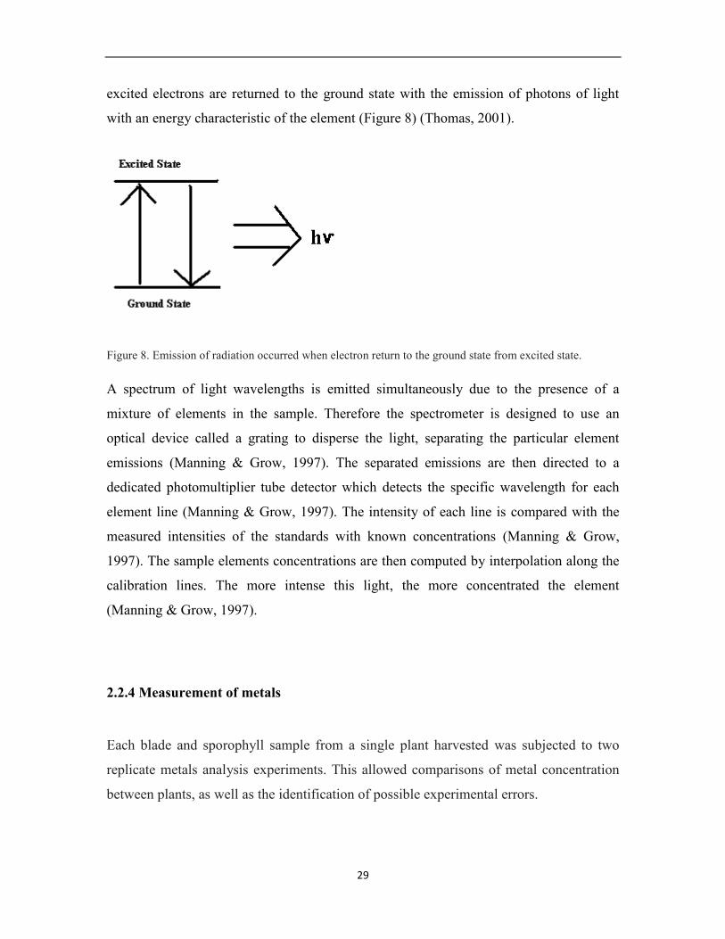
29
excited electrons are returned to the ground state with the emission of photons of light
with an energy characteristic of the element (Figure 8) (Thomas, 2001).
Figure 8. Emission of radiation occurred when electron return to the ground state from excited state.
A spectrum of light wavelengths is emitted simultaneously due to the presence of a
mixture of elements in the sample. Therefore the spectrometer is designed to use an
optical device called a grating to disperse the light, separating the particular element
emissions (Manning & Grow, 1997). The separated emissions are then directed to a
dedicated photomultiplier tube detector which detects the specific wavelength for each
element line (Manning & Grow, 1997). The intensity of each line is compared with the
measured intensities of the standards with known concentrations (Manning & Grow,
1997). The sample elements concentrations are then computed by interpolation along the
calibration lines. The more intense this light, the more concentrated the element
(Manning & Grow, 1997).
2.2.4 Measurement of metals
Each blade and sporophyll sample from a single plant harvested was subjected to two
replicate metals analysis experiments. This allowed comparisons of metal concentration
between plants, as well as the identification of possible experimental errors.

30
The ICP AES was running at Power of 1.2 kW, plasma flow at 15.0 L/min, auxiliary flow
at 1.5 L/min, nebulizer Pressure at 200 kPa, replicate time at 1 second, stability time of
15 seconds and PMT Voltage of 650 V. The ICP AES sample introduction settings was
set at default, sample uptake of 30 seconds, rinse time of 10 seconds and pump rate at 15
rpm.
Different wavelengths were assigned for the ICE AES for measuring concentration of
particular metal; the wavelengths were as followed: As - 193.696 nm, Ca - 396.847 nm,
Cd - 228.803 nm, Cr - 267.716 nm, Cu - 224.700 nm, Hg - 253.652 nm, K - 766.490 nm,
Mg - 285.213 nm, Mn - 260.569 nm, Na - 330.237 nm, Ni - 231.604 nm, P - 213.618 nm,
Pb - 220.353 nm, Se - 196.026 nm and Zn - 206.200 nm. The software applied in
controlling the ICP AES was ICP Expert 4.0 on a Windows Me platform system.
2.2.5 Metal element standards
Commercial standards of 1000 ppm of Ca, Cr, Mg, Mn, Na and Se manufactured by BDH
Ltd and 1000 ppm of As, K, P, Pb and Ni manufactured by Merck Ltd were used. 1000
ppm standard of Cu was made by dissolving 1.000 g of AR graded copper metal in 3mL
of concentrated nitric acid, and then diluted with deionised water to 1 litre in a volumetric
flask. 1000 ppm Zn standard was also prepared with the same method, 1 g of AR graded
pure Zn metal was dissolved in 3 mL of concentrated nitric acid, and then diluted with
deionised water to 1 litre in a volumetric flask. 1000 ppm of Hg standard was made by
dissolving 1.3540 g of HgCl2 in 10 mL of HNO3 followed by dilution to 1 litre in a
volumetric flask with deionised water. 1000 ppm of Cd standard was made by dissolving
2.2819 g of 3CdSO4·8H2O in 250 mL of deionised water and diluted to 1 litre in a
volumetric flask with deionised water.
The above fifteen 1000 ppm metal standards were used to make multi-elements standards
and applied for ICP AES calibrations.

31
2.2.6 Quality control
To maintain the ICP AES reproducibility and standard of the machine wavelength
calibrations and torch cleaning were routinely carried out.
Wavelength calibrations were performed before each month’s analysis. The ICP Expert
program had programmed to calibrate wavelength with the mercury line at first order
with 194.163 nm, 252.652 nm, 365.015 nm, 404.656 nm, 435.833 nm, 546.073 nm, 2nd
order with, 365.015 nm, 404.656 nm, 435.833 nm and 3rd
order with 312.567 nm.
Due to heavy usage of the ICP AES, the torch was cleaned when deposits were noticed
on the surface of the outer cone of the torch. This aimed to prevent torch melt down. To
remove other deposits or stains, the torch was soaked in aqua regia (concentrated nitric
acid: concentrated hydrochloric acid, 1:3 by volume) overnight. Then rinsed well with
water and dried before it was connected back in to the machine. This was followed by
torch alignment programmed in the ICP Expert software.

32
2.3 Pilot studies
Pilot studies were carried out to determine the most timely and economic method with the
available resources.
2.3.1 Comparison of fresh and dried of Undaria pinnatifida digestion
Fresh tissue sample digestion had been adapted to different metal concentration studies in
plant, meat and other organic samples. However a majority of research of metal
concentration in seaweed had been carried out with dried samples. This trial was aimed to
access the possibility of using fresh samples in this research.
Two replicate seaweed samples were (5g wet weight) were cut out from an individual
plant harvested from farm 233 from Pelorus Sound, South Island, New Zealand (41º 09
22.88” S, 173º 51 12.65 E) obtained in May 2011. The two samples were digested in 10
mL of HNO3 for 120 minutes followed by addition of 5 mL HClO4. The experiment was
repeated with the same conditions but with 20 mL HNO3.
2.3.2 Comparison of sample size
Most previous studies used 1g of dried seaweed sample for metal concentration
measurements. In this study, it was important to investigate the optimal amount of
samples to be used to obtain stable reproducible results and to take into consideration that
the sample size might be unpredictable during the sampling period.
Homogenized samples from farm 327 obtained in April 2011 were used. The testing
weights were 0.1 g, 0.25 g, 0.5 g and 1 g. Four sub samples of each trial weight were
taken for digestion. The digestion parameters were identical as the previous trial.

33
2.3.3 Comparison of freeze dried and oven dried samples
While previous studies have shown that there is no difference in metal analyses (Hossain,
N. Canha, M. C. Freitas, Santa Regina, & A. Garcia-Sanche, 2011), whether the samples
are oven dried or freeze dried, as both methods were used in this study, comparison of
these methods on Undaria pinnatifida were carried out.
Three plants from Wellington site B, were used in this trial. The samples were briefly
washed with de-ionized water to remove possible remaining debris. The two sides of the
blade of each plant were separated from the mid stipe. The two half blades of each plant
were then subjected to oven dry and freeze dry pretreatment respectively. The oven
drying process was carried out at 60°C in a Sanyo MOV-112 laboratory oven for 72
hours and the freeze drying process was carried in a Christ Alpha 2-4 freeze drier at -
20°C for 72 hours. The samples were grounded to fine powder by a blender and stored in
clean polystyrene bottles to await analysis. Each sample was subject to two metal
analysis experiments. The digestion and analysis procedures used were identical to
section 2.2.1 and 2.2.2.
2.4 Statistical analysis
All statistical analysis were carried out with Minitab 14 software and graphs were created
with Microsoft excel 2007 software.
2.4.1 Statistical analysis for pilot studies
One way ANOVA was used to compare sample size experiments to determine the
appropriate sample size to be used in the acid digestion. A Paired T test was used in the
comparison of freeze dried versus oven dried experiment to determine differences.

34
2.4.2 Statistical analysis for main study
A one way ANOVA analysis of farm PE 327 was employed to examine seasonal
differences in metal concentrations, as this site contained the most amount and frequent
data. Comparisons between site and time employed a two way ANOVA for data from
August to October as these three months had contained data from all four locations. All
fifteen metals analysis data from PE 327 were also used to perform paired T- tests to
determine the difference in metal concentrations between the blade and sporophyll tissue.

35
Chapter 3 Results
3.1 Pilot studies results
3.1.1 Comparison of fresh versus dried sample digestion
The digestion could not produce an ideal effect to dissolve the sample. The reaction did
not appear to be violent as expected with very little brown fume released from the
mixtures. Also during the filtering process fragments of tissue believed to be un-dissolved
fiber were identified. These phenomena indicated the oxidizing ability of the nitric acid
did not take place as expected. This is caused by large water content in the fresh tissue of
the seaweed which diluted the acidity of the solution. Fresh Undaria pinnatifida has
water content of more than 80%.
The experiment with 20 mL HNO3 caused digestions that were more violent with
reasonable amount of brown fume produced. But un-dissolved fibers were also observed
in the mixture. Therefore fresh samples were not used in this study due to the amount of
HNO3 needed and the amount of un-dissolved tissues. Dried pulverized samples were
used, because dried sample had most of their organic structures destroyed in the drying
process and dried powder provided more surface area for the acid to digest the sample.

36
3.1.2 Comparison of sample size
The one way ANOVA tests showed significant difference for all metals between the four
sample sizes. Tukey’s comparison of means indicated that there was no difference
between 1g and 0.5g of sample in the acid digestion step (Appendix 1). So for the
remaining analysis 0.5 g was used.
3.1.3 Comparison of freeze dried versus oven dried samples
Paired T-test of all metals showed no significant difference between the results obtained
from digestions of freeze dried and oven dried samples (Appendix 2).
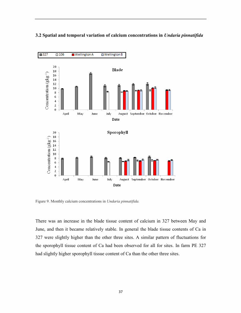
37
3.2 Spatial and temporal variation of calcium concentrations in Undaria pinnatifida
Figure 9. Monthly calcium concentrations in Undaria pinnatifida.
There was an increase in the blade tissue content of calcium in 327 between May and
June, and then it became relatively stable. In general the blade tissue contents of Ca in
327 were slightly higher than the other three sites. A similar pattern of fluctuations for
the sporophyll tissue content of Ca had been observed for all for sites. In farm PE 327
had slightly higher sporophyll tissue content of Ca than the other three sites.

38
Table 3. Results of One-way ANOVA testing for differences in farm PE327 for calcium concentrations
between months for both blade and sporophyll tissue
Blade Source DF SS MS F P
time 6 134.690 22.448 62.41 0.000
Error 53 19.063 0.360
Total 59 153.753
S = 0.5997 R-Sq = 87.60% R-Sq(adj) = 86.20%
Sporophyll Source DF SS MS F P
time 6 3.679 0.613 4.38 0.001
Error 53 7.425 0.140
Total 59 11.103
S = 0.3743 R-Sq = 33.13% R-Sq(adj) = 25.56%
There was a significant difference (P < 0.001) between the blade tissue content of
calcium in farm PE 327 across the seven months study (Table 3). The Tukey’s
comparison of means showed that there were statistical differences between the monthly
means of the blade content of Ca in PE 327. However this was not enough to suggest that
clear seasonal trend.
There was a significant difference (P < 0.05) between the sporophyll tissue content of Ca
in farm PE 327 across the seven months study (Table 3). The Tukey’s comparison of
means showed that there were statistical differences between the monthly means of the
sporophyll tissue content of Ca in PE 327. However this was not enough to suggest a
clear seasonal trend.

39
Table 4. Two way analysis of Variance of calcium in the period between August and October for blade and
sporophyll tissue
Blade Source DF SS MS F P
Site id 3 193.529 64.5096 295.79 0.000
time 2 28.490 14.2451 65.32 0.000
Interaction 6 6.504 1.0840 4.97 0.000
Error 132 28.788 0.2181
Total 143 257.311
S = 0.4670 R-Sq = 88.81% R-Sq(adj) = 87.88%
Sporophyll Source DF SS MS F P
Site id 3 59.8962 19.9654 133.22 0.000
time 2 3.5724 1.7862 11.92 0.000
Interaction 6 0.6656 0.1109 0.74 0.618
Error 132 19.7830 0.1499
Total 143 83.9172
S = 0.3871 R-Sq = 76.43% R-Sq(adj) = 74.46%
Table 4 shows that there were significant differences between both time and site for the
blade tissue content of calcium. There was also significant interaction between these two
parameters indicated that they did not vary in a systematic manner. A difference pattern
was found for the sposophyll where there were significant differences between both site
and time but no interaction between the two parameters.

40
Table 5. Comparison of the blade and sporophyll tissue content of calcium
Paired T for Ca(g/kg) Blade - Ca(g/kg) Sporophyll
N Mean StDev SE Mean
Ca(g/kg) Blade 60 11.8137 1.6143 0.2084
Ca(g/kg) Sporoph 60 8.3511 0.4338 0.0560
Difference 60 3.46253 1.48283 0.19143
95% CI for mean difference: (3.07948, 3.84559)
T-Test of mean difference = 0 (vs not = 0): T-Value = 18.09 P-Value = 0.000
Table 5 shows that there was significant difference of calcium content between the blade
and sporophyll tissue from farm 327. In farm 327, the blade tissue had content of Ca on
average between 3.07 and 3.84 g kg-1
higher than the sporophyll tissue.

41
3.3 Spatial and temporal variation of potassium concentrations in Undaria
pinnatifida
Figure 10. Monthly potassium concentrations in Undaria pinnatifida.
There were steady increases of blade content of potassium in PE 327 from April to
October, a similar trend also observed along the sampling period in farm 106 and both
wellington sites between August and October. A similar pattern of fluctuations of the
sporophyll tissue content of K had been observed for all for sites but the sporophyll
content of K in 106 had noticeable lower concentration than the other three sites.

42
Table 6. Results of a One-way ANOVA testing for differences in farm PE327 for potassium concentrations
between months in both blade and sporophyll tissue.
Blade Source DF SS MS F P
time 5 4026.94 805.39 503.43 0.000
Error 50 79.99 1.60
Total 55 4106.93
S = 1.265 R-Sq = 98.05% R-Sq(adj) = 97.86%
Sporophyll Source DF SS MS F P
time 5 22.465 4.493 5.43 0.000
Error 50 41.404 0.828
Total 55 63.869
S = 0.9100 R-Sq = 35.17% R-Sq(adj) = 28.69%
There was significant difference (P < 0.001) between the blade tissue content of
potassium in farm PE 327 across the seven months study (Table 6). The Tukey’s
comparison of means showed that there were statistical differences between the monthly
means of the blade tissue content of K in farm PE 327. This suggested that there was a
possible seasonal trend
There was significant difference (P < 0.001) between the sporophyll tissue content of K
in farm PE 327 across the seven months study (Table 6). The Tukey’s comparison of
means showed that there were statistical differences between the monthly means of the
sporophyll content of K in farm PE 327. However this evidence was not significant to
suggest that there was a clear seasonal trend.

43
Table 7. Two way analysis of Variance of potassium in the period between August and October for blade
and sporophyll tissue.
Blade Source DF SS MS F P
Site id 3 392.28 130.76 210.35 0.000
time 2 6270.62 3135.31 5043.64 0.000
Interaction 6 1393.89 232.31 373.72 0.000
Error 132 82.06 0.62
Total 143 8138.85
S = 0.7884 R-Sq = 98.99% R-Sq(adj) = 98.91%
Sporophyll Source DF SS MS F P
Site id 3 3802.47 1267.49 2187.61 0.000
time 2 26.52 13.26 22.88 0.000
Interaction 6 18.22 3.04 5.24 0.000
Error 132 76.48 0.58
Total 143 3923.68
S = 0.7612 R-Sq = 98.05% R-Sq(adj) = 97.89%
Table 7 shows that there was significant differences for both time and site for the blade
tissue content of potassium. There was also a significant interaction between these two
parameters indicated that they did not vary in a systematic manner. A similar pattern was
found for sporophyll, where there were signifcant differences for both site and time for
the sporophyll content of K. There was also a significant interaction between these two
parameters indicated that they did not vary in a systematic manner.
Table 8. Comparison of the blade and sporophyll tissue content of potassium
Paired T for K(g/kg) Blade - K(g/kg) Sporophyll
N Mean StDev SE Mean
K(g/kg) Blade 56 32.9044 8.6413 1.1547
K(g/kg) Sporophy 56 27.5811 1.0776 0.1440
Difference 56 5.32329 8.75369 1.16976
95% CI for mean difference: (2.97903, 7.66754)
T-Test of mean difference = 0 (vs not = 0): T-Value = 4.55 P-Value = 0.000
Table 8 shows that there was significant difference of potassium content between the
blade and sporophyll tissue from farm 327. In farm 327, the blade tissue had content of K
on average between 2.98 and 7.67 g kg-1
higher than the sporophyll tissue.

44
3.4 Spatial and temporal variation of magnesium concentrations in Undaria
pinnatifida
Figure 11. Monthly magnesium concentrations in Undaria pinnatifida.
There was an increasing trend for the blade tissue content of magnesium in PE 327
between April and October. The blade tissue contents of Mg in August to October were
very similar between the four sites. There was also an increasing trend between April and
October for the sporophyll tissue content of Mg in PE 327. The other three sites had
shown some fluctuations of sporophyll tissue content of Mg, in which Wellington B site
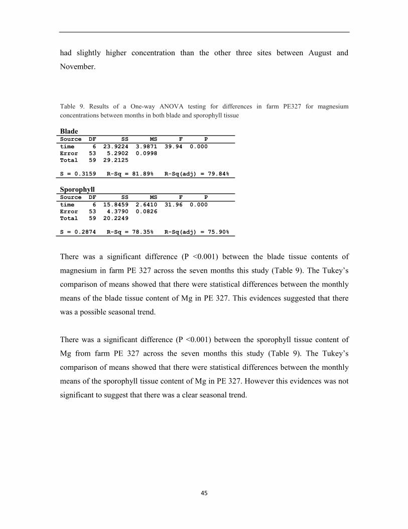
45
had slightly higher concentration than the other three sites between August and
November.
Table 9. Results of a One-way ANOVA testing for differences in farm PE327 for magnesium
concentrations between months in both blade and sporophyll tissue
Blade Source DF SS MS F P
time 6 23.9224 3.9871 39.94 0.000
Error 53 5.2902 0.0998
Total 59 29.2125
S = 0.3159 R-Sq = 81.89% R-Sq(adj) = 79.84%
Sporophyll Source DF SS MS F P
time 6 15.8459 2.6410 31.96 0.000
Error 53 4.3790 0.0826
Total 59 20.2249
S = 0.2874 R-Sq = 78.35% R-Sq(adj) = 75.90%
There was a significant difference (P <0.001) between the blade tissue contents of
magnesium in farm PE 327 across the seven months this study (Table 9). The Tukey’s
comparison of means showed that there were statistical differences between the monthly
means of the blade tissue content of Mg in PE 327. This evidences suggested that there
was a possible seasonal trend.
There was a significant difference (P <0.001) between the sporophyll tissue content of
Mg from farm PE 327 across the seven months this study (Table 9). The Tukey’s
comparison of means showed that there were statistical differences between the monthly
means of the sporophyll tissue content of Mg in PE 327. However this evidences was not
significant to suggest that there was a clear seasonal trend.
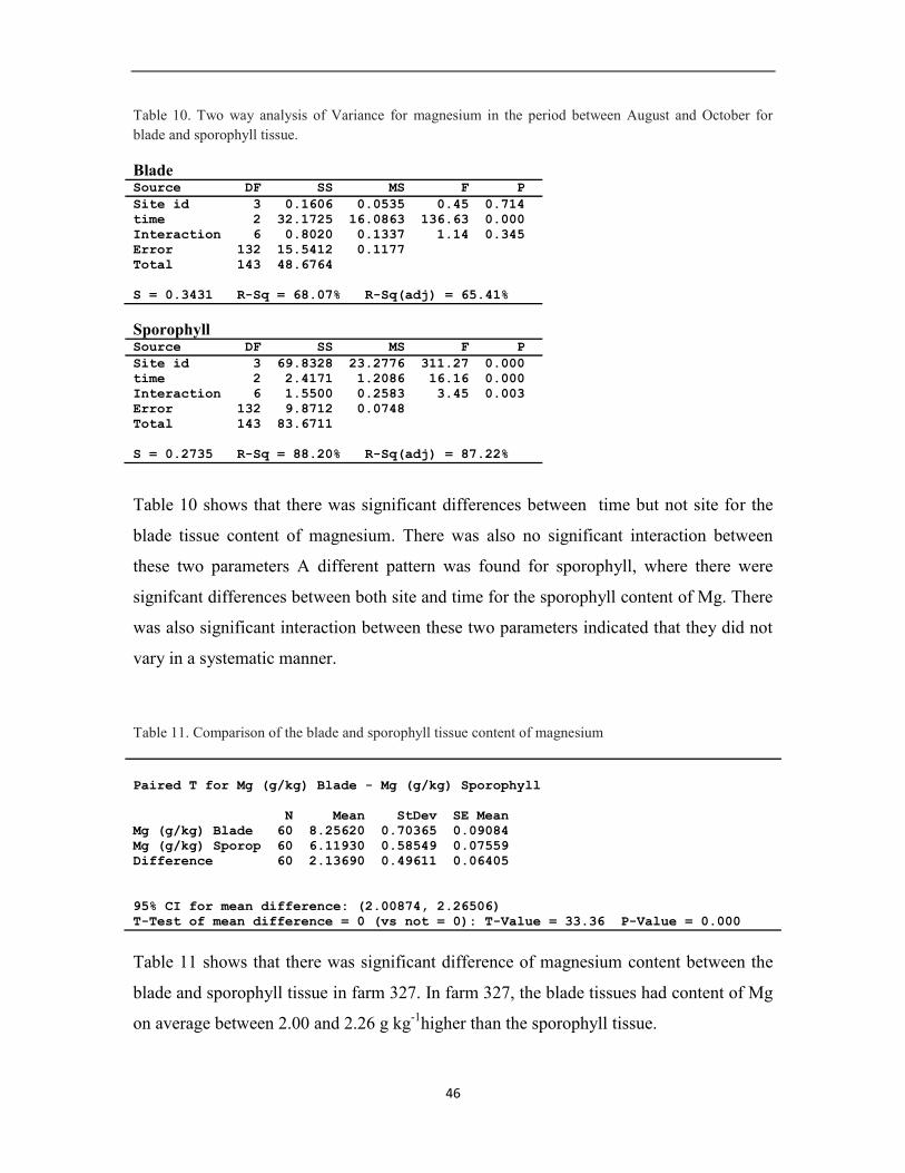
46
Table 10. Two way analysis of Variance for magnesium in the period between August and October for
blade and sporophyll tissue.
Blade Source DF SS MS F P
Site id 3 0.1606 0.0535 0.45 0.714
time 2 32.1725 16.0863 136.63 0.000
Interaction 6 0.8020 0.1337 1.14 0.345
Error 132 15.5412 0.1177
Total 143 48.6764
S = 0.3431 R-Sq = 68.07% R-Sq(adj) = 65.41%
Sporophyll Source DF SS MS F P
Site id 3 69.8328 23.2776 311.27 0.000
time 2 2.4171 1.2086 16.16 0.000
Interaction 6 1.5500 0.2583 3.45 0.003
Error 132 9.8712 0.0748
Total 143 83.6711
S = 0.2735 R-Sq = 88.20% R-Sq(adj) = 87.22%
Table 10 shows that there was significant differences between time but not site for the
blade tissue content of magnesium. There was also no significant interaction between
these two parameters A different pattern was found for sporophyll, where there were
signifcant differences between both site and time for the sporophyll content of Mg. There
was also significant interaction between these two parameters indicated that they did not
vary in a systematic manner.
Table 11. Comparison of the blade and sporophyll tissue content of magnesium
Paired T for Mg (g/kg) Blade - Mg (g/kg) Sporophyll
N Mean StDev SE Mean
Mg (g/kg) Blade 60 8.25620 0.70365 0.09084
Mg (g/kg) Sporop 60 6.11930 0.58549 0.07559
Difference 60 2.13690 0.49611 0.06405
95% CI for mean difference: (2.00874, 2.26506)
T-Test of mean difference = 0 (vs not = 0): T-Value = 33.36 P-Value = 0.000
Table 11 shows that there was significant difference of magnesium content between the
blade and sporophyll tissue in farm 327. In farm 327, the blade tissues had content of Mg
on average between 2.00 and 2.26 g kg-1
higher than the sporophyll tissue.

47
3.5 Spatial and temporal variation of sodium concentrations in Undaria pinnatifida
Figure 12. Monthly sodium concentrations in Undaria pinnatifida.
There was a steady increase of the blade content of sodium between April and July in PE
327, and followed by small fluctuations near the end of the sampling period. The blade
contents of Na from Port Underwood were higher than sites from Wellington. There was
also a steady increase of the sporophyll content of Na between April and July from PE
327 and followed by small fluctuations toward end of the sampling period. The
sporophyll Na levels from Port Underwood were higher than sites from Wellington.

48
Table 12. Results of One-way ANOVA testing for differences in farm PE327 for sodium concentrations
between months in both blade and sporophyll tissue
Blade Source DF SS MS F P
time 6 18542.20 3090.37 3090.51 0.000
Error 53 53.00 1.00
Total 59 18595.19
S = 1.000 R-Sq = 99.71% R-Sq(adj) = 99.68%
Sporophyll Source DF SS MS F P
time 6 2148.485 358.081 1112.94 0.000
Error 53 17.052 0.322
Total 59 2165.538
S = 0.5672 R-Sq = 99.21% R-Sq(adj) = 99.12%
There was significant difference (P < 0.001) between the blade tissue content of sodium
in farm PE 327 across the seven months study (Table 12). The Tukey’s comparison of
means showed that there were statistical differences between the monthly means of the
blade tissue content of Na in farm PE 327. This was not enough to suggest a clear
seasonal trend.
There was significant difference (P < 0.001) between the sporophyll tissue content of Na
in farm PE 327 across the seven months study (Table 12). The Tukey’s comparison of
means showed that there were statistical differences between the monthly means of the
sporophyll tissue content of Na in farm PE 327. This was not enough to suggest a clear
seasonal trend.

49
Table 13. Two way analysis of Variance for sodium in the period between August and October for blade
and sporophyll tissue
Blade Source DF SS MS F P
Site id 3 40938.6 13646.2 26624.03 0.000
time 2 239.0 119.5 233.18 0.000
Interaction 6 93.8 15.6 30.51 0.000
Error 132 67.7 0.5
Total 143 41339.1
S = 0.7159 R-Sq = 99.84% R-Sq(adj) = 99.82%
Sporophyll Source DF SS MS F P
Site id 3 4887.96 1629.32 5812.30 0.000
time 2 15.41 7.70 27.48 0.000
Interaction 6 57.33 9.55 34.09 0.000
Error 132 37.00 0.28
Total 143 4997.70
S = 0.5295 R-Sq = 99.26% R-Sq(adj) = 99.20%
Table 13 shows that there was significant differences for both time and site for the blade
tissue content of sodium. There was also a significant interaction between these two
parameters indicated that they did not vary in a systematic manner. A similar pattern was
also found for sporophyll, where there were signifcant differences between both site and
time for the sporophyll content of Na. There was also a significant interaction between
these two parameters indicated that they did not vary in a systematic manner.
Table 14 shows that there was significant difference of sodium content between the blade
and sporophyll tissue in farm 327. In farm 327, the blade tissue had content of Na on
average between 22.64 and 28.92 g kg-1
higher than the sporophyll tissue.

50
Table 14. Comparison of blade and sporophyll tissue content of sodium
Paired T for Na (g/kg) Blade - Na (g/kg) Sporophyll
N Mean StDev SE Mean
Na (g/kg) Blade 60 54.1961 17.7531 2.2919
Na (g/kg) Sporop 60 28.4114 6.0584 0.7821
Difference 60 25.7847 12.1730 1.5715
95% CI for mean difference: (22.6401, 28.9293)
T-Test of mean difference = 0 (vs not = 0): T-Value = 16.41 P-Value = 0.000
3.6 Spatial and temporal variation of phosphorus concentrations in Undaria
pinnatifida
Figure 13. Monthly phosphorus concentrations in Undaria pinnatifida.

51
A pattern of fluctuations without noticeable trend for the blade tissue content of
phosphorus had been observed from all four sites. A similar pattern was also observed for
the sporophyll tissue content of P.
Table 15. Results of a One-way ANOVA testing for differences in farm PE327 for phosphorus
concentrations between months in both blade and sporophyll tissue.
Blade Source DF SS MS F P
time 5 35.558 7.112 34.48 0.000
Error 50 10.313 0.206
Total 55 45.871
S = 0.4542 R-Sq = 77.52% R-Sq(adj) = 75.27%
Sporophyll Source DF SS MS F P
time 5 10.602 2.120 12.68 0.000
Error 50 8.360 0.167
Total 55 18.963
S = 0.4089 R-Sq = 55.91% R-Sq(adj) = 51.50%
There was significant difference (P < 0.001) between the blade tissue content of
phosphorus in farm PE 327 across the seven months study (Table 15). The Tukey’s
comparison of means showed that there were statistical differences between the monthly
means of the blade tissue content of P in farm PE 327. However, this evidence was not
significant to suggest that there was a clear seasonal trend.
There was significant difference (P < 0.001) between the sporophyll tissue content of P in
farm PE 327 across the seven months study (Table 15). The Tukey’s comparison of
means showed that there were statistical differences between the monthly means of the
sporophyll tissue content of P in farm PE 327. However, this evidence was not
significant to suggest that there was a clear seasonal trend.

52
Table 16. Two way analysis of Variance of phosphorus in the period between August and October for blade
and sporophyll tissue.
Blade
Source DF SS MS F P
Site id 3 68.730 22.9100 97.33 0.000
time 2 59.909 29.9544 127.26 0.000
Interaction 6 4.078 0.6796 2.89 0.011
Error 132 31.070 0.2354
Total 143 163.787
S = 0.4852 R-Sq = 81.03% R-Sq(adj) = 79.45%
Sporophyll Source DF SS MS F P
Site id 3 55.5153 18.5051 159.52 0.000
time 2 7.1377 3.5688 30.76 0.000
Interaction 6 3.0148 0.5025 4.33 0.001
Error 132 15.3129 0.1160
Total 143 80.9807
S = 0.3406 R-Sq = 81.09% R-Sq(adj) = 79.51%
Table 43 shows that there was significant differences for both time and site for the blade
tissue content of phosphorus. There was also a significant interaction between these two
parameters indicated that they did not vary in a systematic manner. A similar pattern was
found for sporophyll, where there were signifcant differences for both site and time for
the sporophyll content of P. There was also a significant interaction between these two
parameters indicated that they did not vary in a systematic manner.
Table 17. Comparison of the blade and sporophyll tissue content of phosphorus
Paired T for P(g/kg) Blade - P(g/kg) Sporophyll
N Mean StDev SE Mean
P(g/kg) Blade 56 10.7452 0.9132 0.1220
P(g/kg) Sporophy 56 8.8129 0.5872 0.0785
Difference 56 1.93232 0.75554 0.10096
95% CI for mean difference: (1.72999, 2.13466)
T-Test of mean difference = 0 (vs not = 0): T-Value = 19.14 P-Value = 0.000
Table 17 shows that there was significant difference of phosphorus content between the
blade and sporophyll tissue in farm 327. In farm 327, the blade tissue had content of P on
average between 1.72 and 2.13 g kg-1
higher than the sporophyll tissue.

53
3.7 Spatial and temporal variation of chromium concentrations in Undaria
pinnatifida
Figure 14. Monthly chromium concentrations in Undaria pinnatifida.
There was an increasing trend between April and June for the blade tissue content of
chromium in farm PE 327, it became relative stable till September and ended with
another small increase in October. The blade tissue content of Cr from the other three
sites had shown some fluctuations during their sampling period. There was also an
increasing trend between April and June for the sporophyll tissue content of Cr in farm
PE 327, it became relative stable to the end of its sampling period. The sporophyll tissue

54
contents of Cr in the other three sites were steady and had shown some fluctuations
during their sampling periods.
Table 18. Results of a One-way ANOVA testing for differences in farm PE327 for chromium
concentrations between months in both blade and sporophyll tissue
Blade Source DF SS MS F P
time 6 0.4246 0.0708 2.96 0.014
Error 53 1.2674 0.0239
Total 59 1.6921
S = 0.1546 R-Sq = 25.10% R-Sq(adj) = 16.62%
Sporophyll Source DF SS MS F P
time 6 0.10179 0.01696 5.30 0.000
Error 53 0.16965 0.00320
Total 59 0.27144
S = 0.05658 R-Sq = 37.50% R-Sq(adj) = 30.42%
There was a significant difference (P < 0.05) between the blade tissue content of
chromium in farm PE 327 across the seven months study (Table 18). The Tukey’s
comparison of means showed that there were statistical differences between the monthly
means of the blade tissue content of Cr in farm PE 327. However this evidence was not
significant to suggest that there was a clear seasonal trend.
There was a significant difference (P < 0.001) between the sporophyll tissue content of
Cr in farm PE 327 across the seven months study (Table 18). The Tukey’s comparison of
means showed that there were statistical differences between the monthly means of the
sporophyll tissues content of Cr in farm PE 327. However, this evidence was not
significant to suggest that there was a clear seasonal trend.

55
Table 19. Two way analysis of Variance for chromium in the period between August and October for blade
and sporophyll tissue
Blade Source DF SS MS F P
Site id 3 1.67301 0.557669 44.69 0.000
time 2 0.09784 0.048918 3.92 0.022
Interaction 6 0.04333 0.007221 0.58 0.747
Error 132 1.64712 0.012478
Total 143 3.46129
S = 0.1117 R-Sq = 52.41% R-Sq(adj) = 48.45%
Sporophyll Source DF SS MS F P
Site id 3 0.272493 0.0908309 33.16 0.000
time 2 0.024584 0.0122919 4.49 0.013
Interaction 6 0.021059 0.0035098 1.28 0.270
Error 132 0.361551 0.0027390
Total 143 0.679686
S = 0.05234 R-Sq = 46.81% R-Sq(adj) = 42.37%
Table 19 shows that there were significant differences between for both site but time for
the blade tissue content of chromium but no interaction between the two parameters. A
similar pattern was also found for sporophyll, where there were signifcant differences
between both site and time for the sporophyll content of Cr but no interaction between the
two parameters.
Table 20 shows that there was significant difference of chromium content between the
blade and sporophyll tissue in farm 327. In farm 327, the blade tissues had content of Cr
on average between 0.098 and 0.188 mg kg-1
higher than the sporophyll tissue.

56
Table 20. Comparison of the blade and sporophyll tissue content of chromium
Paired T for Cr Blade - Cr Sporophyll
N Mean StDev SE Mean
Cr Blade 60 0.938550 0.169348 0.021863
Cr Sporophyll 60 0.795067 0.067828 0.008757
Difference 60 0.143483 0.172580 0.022280
95% CI for mean difference: (0.098901, 0.188066)
T-Test of mean difference = 0 (vs not = 0): T-Value = 6.44 P-Value = 0.000
3.8 Spatial and temporal variation of copper concentrations in Undaria pinnatifida
Figure 15. Monthly copper concentrations in Undaria pinnatifida.

57
The blade tissue contents of copper in the sites of Port Underwood were similar and were
higher than the two sites from wellington. There was a clear decreasing trend of the blade
tissue content of Cu between April and July in farm PE 327, and the trend became
positive between July and October. The blade tissue content of Cu in the other three sites
had small fluctuations and relative stable during their sampling period. The sporophyll
tissue content of Cu from all four sites had shown some fluctuations during their
sampling period with no noticeable trend observed.
Table 21. Results of a One-way ANOVA testing for differences in farm PE327 for copper concentrations
between months in both blade and sporophyll tissue.
Blade Source DF SS MS F P
time 6 4.2047 0.7008 9.42 0.000
Error 53 3.9408 0.0744
Total 59 8.1455
S = 0.2727 R-Sq = 51.62% R-Sq(adj) = 46.14%
Sporophyll Source DF SS MS F P
time 6 0.4961 0.0827 2.61 0.027
Error 53 1.6769 0.0316
Total 59 2.1730
S = 0.1779 R-Sq = 22.83% R-Sq(adj) = 14.09%
There was a significant difference (P < 0.001) between the blade tissue content of copper
in farm PE 327 across the seven months of study (Table 21). The Tukey’s comparison of
means showed that there were statistical differences between the monthly means of the
blade tissue content of Cu in farm PE 327. However, this evidence was not significant to
suggest that there was a clear seasonal trend.
There was a significant difference (P < 0.05) between the sporophyll tissue content of Cu
in farm PE 327 across the seven months of study (Table 21). The Tukey’s comparison of
means did not show that there were statistical differences between the monthly means of
the sporophyll tissue content of Cu in PE 327. However, this evidence was not significant
to suggest that there was a clear seasonal trend.

58
Table 22. Two way analysis of Variance for copper in the period between August and October for blade
and sporophyll tissue.
Blade Source DF SS MS F P
Site id 3 32.3905 10.7968 117.31 0.000
time 2 4.1339 2.0669 22.46 0.000
Interaction 6 1.6708 0.2785 3.03 0.008
Error 132 12.1490 0.0920
Total 143 50.3441
S = 0.3034 R-Sq = 75.87% R-Sq(adj) = 73.86%
Sporophyll Source DF SS MS F P
Site id 3 12.7306 4.24352 79.77 0.000
time 2 1.4414 0.72069 13.55 0.000
Interaction 6 0.8850 0.14749 2.77 0.014
Error 132 7.0219 0.05320
Total 143 22.0788
S = 0.2306 R-Sq = 68.20% R-Sq(adj) = 65.55%
Table 22 shows that there were significant differences between for both site but time for
the blade tissue content of copper. There was also significant interaction between these
two parameters indicated that they did not vary in a systematic manner. A similar pattern
was also found for sporophyll, where there were signifcant differences between both site
and time for the sporophyll content of Cu. There was also significant interaction between
these two parameters indicated that they did not vary in a systematic manner.
Table 23. Comparison of the blade and sporophyll tissue content of copper
Paired T for Cu Blade - Cu Sporophyll
N Mean StDev SE Mean
Cu Blade 60 3.40518 0.37156 0.04797
Cu Sporophyll 60 1.73138 0.19191 0.02478
Difference 60 1.67380 0.43096 0.05564
95% CI for mean difference: (1.56247, 1.78513)
T-Test of mean difference = 0 (vs not = 0): T-Value = 30.08 P-Value = 0.000

59
Table 23 shows that there was significant difference of copper content between the blade
and sporophyll tissue in farm 327. In farm 327, the blade tissue had content of Cu on
average between 1.56 and 1.78 mg kg-1
higher than the sporophyll tissue.
3.9 Spatial and temporal variation of manganese concentrations in Undaria
pinnatifida
Figure 16. Monthly manganese concentrations in Undaria pinnatifida.
There were small fluctuations for the blade tissue content of manganese in all four sites
during the sampling period. However the blade tissues in Wellington site A had higher
Mn content than the other three sites. All four sites showed fluctuations for the sporophyll

60
tissue content of Mn. It is noteworthy the sporophyll content of Mn in Wellington sites
were higher than the Port Underwood sites.
Table 24. Results of One-way ANOVA testing for differences in farm PE327 for manganese concentrations
between months in both blade and sporophyll tissue
Blade Source DF SS MS F P
time 6 23.99 4.00 0.83 0.555
Error 53 256.54 4.84
Total 59 280.53
S = 2.200 R-Sq = 8.55% R-Sq(adj) = 0.00%
Sporophyll Source DF SS MS F P
time 6 42.341 7.057 31.06 0.000
Error 53 12.043 0.227
Total 59 54.384
S = 0.4767 R-Sq = 77.86% R-Sq(adj) = 75.35%
There was no difference (P > 0.10) between the blade tissue content of manganese in
farm PE 327 across the seven months study (Table 24). The Tukey’s comparison of
means did not show that there were statistical differences between the monthly means of
the blade tissue content of Mn in PE 327. This evidence was not significant to suggest
that there was a clear seasonal trend.
There was a significant difference (P < 0.001) between the sporophyll tissue content of
Mn in farm PE 327 across the seven months study (Table 24). The Tukey’s comparison
of means showed that there were statistical differences between the monthly means of the
sporophyll tissue content of Mn in farm PE 327. However, this evidence was not
significant to suggest that there was a clear seasonal trend.

61
Table 25. Two way analysis of Variance for manganese in the period between August and October for
blade and sporophyll tissue
Blade Source DF SS MS F P
Site id 3 520.10 173.367 48.17 0.000
time 2 27.21 13.604 3.78 0.025
Interaction 6 30.69 5.115 1.42 0.211
Error 132 475.05 3.599
Total 143 1053.05
S = 1.897 R-Sq = 54.89% R-Sq(adj) = 51.13%
Sporophyll Source DF SS MS F P
Site id 3 169.195 56.3982 186.75 0.000
time 2 4.298 2.1490 7.12 0.001
Interaction 6 0.168 0.0280 0.09 0.997
Error 132 39.864 0.3020
Total 143 213.525
S = 0.5495 R-Sq = 81.33% R-Sq(adj) = 79.77%
Table 25 shows that there was significant differences for both time and site for the blade
tissue content of manganese There was no significant interaction between these two
parameters A similar pattern was also found for sporophyll, where there were signifcant
differences between both site and time for the sporophyll content of Mn. There was also
no significant interaction between these two parameters.
Table 26. Comparison of the blade and sporophyll tissue content of manganese
Paired T for Mn Blade - Mn Sporophyll
N Mean StDev SE Mean
Mn Blade 60 9.47908 2.18055 0.28151
Mn Sporophyll 60 5.44703 0.96009 0.12395
Difference 60 4.03205 2.31623 0.29902
95% CI for mean difference: (3.43370, 4.63040)
T-Test of mean difference = 0 (vs not = 0): T-Value = 13.48 P-Value = 0.000
Table 26 shows that there was significant difference of manganese content between the
blade and sporophyll tissue in farm 327. In farm 327, the blade tissue had content of Mn
on average between 2.32 and 4.63 mg kg-1
higher than the sporophyll tissue.
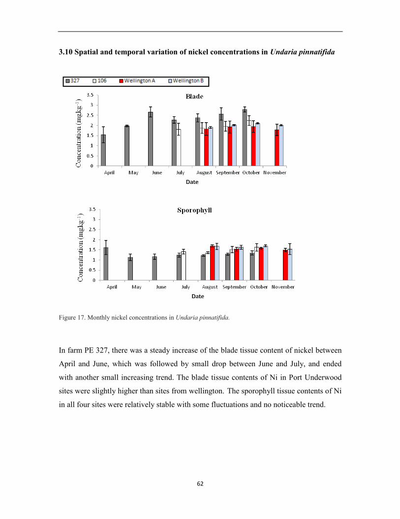
62
3.10 Spatial and temporal variation of nickel concentrations in Undaria pinnatifida
Figure 17. Monthly nickel concentrations in Undaria pinnatifida.
In farm PE 327, there was a steady increase of the blade tissue content of nickel between
April and June, which was followed by small drop between June and July, and ended
with another small increasing trend. The blade tissue contents of Ni in Port Underwood
sites were slightly higher than sites from wellington. The sporophyll tissue contents of Ni
in all four sites were relatively stable with some fluctuations and no noticeable trend.

63
Table 27. Results of One-way ANOVA testing for differences in farm PE327 for nickel concentrations
between months in both blade and sporophyll tissue
Blade Source DF SS MS F P
time 6 6.2898 1.0483 14.53 0.000
Error 53 3.8247 0.0722
Total 59 10.1145
S = 0.2686 R-Sq = 62.19% R-Sq(adj) = 57.91%
Sporophyll Source DF SS MS F P
time 6 0.6938 0.1156 5.12 0.000
Error 53 1.1963 0.0226
Total 59 1.8901
S = 0.1502 R-Sq = 36.71% R-Sq(adj) = 29.54%
There was significant difference (P < 0.001) between the blade tissue content of nickel in
farm PE 327 across the seven months study (Table 27). The Tukey’s comparison of
means showed that there were statistical differences between the monthly means of the
blade tissue content of Ni in farm PE 327. However, this evidence was not significant to
suggest that there was a clear seasonal trend.
There was significant difference (P < 0.001) between the sporophyll tissue content of
nickel in farm PE 327 across the seven months study (Table 27). The Tukey’s
comparison of means showed that there were statistical differences between the monthly
means of the sporophyll tissue content of Ni in farm PE 327. However, this evidence was
not significant to suggest that there was a clear seasonal trend.

64
Table 28. Two way analysis of Variance of nickel in the period between August and October for blade and
sporophyll tissue
Blade Source DF SS MS F P
Site id 3 10.0308 3.34360 78.92 0.000
time 2 1.7838 0.89188 21.05 0.000
Interaction 6 0.4122 0.06871 1.62 0.146
Error 132 5.5922 0.04237
Total 143 17.8190
S = 0.2058 R-Sq = 68.62% R-Sq(adj) = 66.00%
Sporophyll Source DF SS MS F P
Site id 3 2.89268 0.964226 34.24 0.000
time 2 0.16655 0.083275 2.96 0.055
Interaction 6 0.54317 0.090528 3.21 0.006
Error 132 3.71739 0.028162
Total 143 7.31979
S = 0.1678 R-Sq = 49.21% R-Sq(adj) = 44.98%
Table 28 shows that there was significant differences for both time and site for the blade
tissue content of nickel. However there was no significant interaction between these two
parameters. A different pattern was also found for sporophyll, where there were
signifcant differences between site but not time for the sporophyll content of Ni. There
was also a significant interaction between these two parameters indicated that they did
not vary in a systematic manner.
Table 29. Comparison of the blade and sporophyll tissue content of nickel
Paired T for Ni Blade - Ni Sporophyll
N Mean StDev SE Mean
Ni Blade 60 2.41158 0.41404 0.05345
Ni Sporophyll 60 1.28592 0.17899 0.02311
Difference 60 1.12567 0.48383 0.06246
95% CI for mean difference: (1.00068, 1.25065)
T-Test of mean difference = 0 (vs not = 0): T-Value = 18.02 P-Value = 0.000
Table 29 shows that there was significant difference of nickel content between the blade
and sporophyll tissue in farm 327. In farm 327, the blade tissue had content of Ni on
average between 1.00 and 1.25 mg kg-1
higher than the sporophyll tissue.

65
3.11 Spatial and temporal variation of selenium concentrations in Undaria
pinnatifida
Figure 18 Monthly selenium concentrations in Undaria pinnatifida.
The blade tissue contents of selenium in all four sites showed patterns of fluctuation. It is
noticeable that blade tissue in Wellington sites had higher Se content than Port
Underwood sites. The sporophyll tissue content of Se from all four sites also behaved in a
similar manner.

66
Table 30. Results of One-way ANOVA testing for differences in farm PE327 for selenium concentrations
between months in both blade and sporophyll tissue
Blade Source DF SS MS F P
time 6 0.03809 0.00635 5.12 0.000
Error 53 0.06570 0.00124
Total 59 0.10379
S = 0.03521 R-Sq = 36.70% R-Sq(adj) = 29.53%
Sporophyll Source DF SS MS F P
time 6 0.09791 0.01632 8.92 0.000
Error 53 0.09698 0.00183
Total 59 0.19489
S = 0.04278 R-Sq = 50.24% R-Sq(adj) = 44.60%
There was significant difference (P < 0.001) between the blade tissue content of selenium
in farm PE 327 across the seven months study (Table 30). The Tukey’s comparison of
means showed that there were statistical differences between the monthly means of the
blade tissue content of Se in farm PE 327. However, this evidence was not significant to
suggest that there was a clear seasonal trend.
There was significant difference (P < 0.001) between the sporophyll tissue content of
selenium in farm PE 327 across the seven months study (Table 30). The Tukey’s
comparison of means showed that there were statistical differences between the monthly
means of the sporophyll tissue content of Se in farm PE 327. However, this evidence was
not significant to suggest that there was a clear seasonal trend.

67
Table 31. Two way analysis of Variance of selenium in the period between August and October for blade
and sporophyll tissue
Blade Source DF SS MS F P
Site id 3 2.37283 0.790945 116.33 0.000
time 2 0.12754 0.063770 9.38 0.000
Interaction 6 0.13815 0.023026 3.39 0.004
Error 132 0.89749 0.006799
Total 143 3.53602
S = 0.08246 R-Sq = 74.62% R-Sq(adj) = 72.50%
Sporophyll Source DF SS MS F P
Site id 3 0.84878 0.282928 123.13 0.000
time 2 0.02951 0.014753 6.42 0.002
Interaction 6 0.04462 0.007437 3.24 0.005
Error 132 0.30330 0.002298
Total 143 1.22622
S = 0.04793 R-Sq = 75.27% R-Sq(adj) = 73.20%
Table 31 shows that there was significant differences for both time and site for the blade
tissue content of selenium. There was also a significant interaction between these two
parameters indicated that they did not vary in a systematic manner. A similsr pattern was
also found for sporophyll, where there were signifcant differences for both site and time
for the sporophyll content of Se. There was also a significant interaction between these
two parameters indicated that they did not vary in a systematic manner.
Table 32 Comparison of the blade and sporophyll tissue content of Selenium
Paired T for Se Blade - Se Sporophyll
N Mean StDev SE Mean
Se Blade 60 0.565167 0.041943 0.005415
Se Sporophyll 60 0.293650 0.057474 0.007420
Difference 60 0.271517 0.077979 0.010067
95% CI for mean difference: (0.251373, 0.291661)
T-Test of mean difference = 0 (vs not = 0): T-Value = 26.97 P-Value = 0.000
Table 32 shows that there was significant difference of selenium content between the
blade and the sporophyll tissue in farm 327. In farm 327, the blade tissue had content of
Se on average between 0.25 and 0.29 mg kg-1
higher than the sporophyll tissue.

68
3.12 Spatial and temporal variation of zinc concentrations in Undaria pinnatifida
Figure 19. Monthly zinc concentrations in Undaria pinnatifida.
The blade tissue contents of zinc in all four sites showed small fluctuations. Wellington
sites had slightly higher content of blade tissue Zn than Port Underwood sites. The
sporophyll tissue content of Zn in all four sites also showed small flcutuations. It was
noticeable that farm 106 had slightly higher sporophyll tissue content of Zn than the other
three sites.

69
Table 33. Results of One-way ANOVA testing for differences in farm PE327 for zinc concentrations
between months in both blade and sporophyll tissue
Blade Source DF SS MS F P
time 6 140.68 23.45 3.99 0.002
Error 53 311.74 5.88
Total 59 452.42
S = 2.425 R-Sq = 31.09% R-Sq(adj) = 23.29%
Sporophyll Source DF SS MS F P
time 6 109.17 18.19 8.14 0.000
Error 53 118.42 2.23
Total 59 227.59
S = 1.495 R-Sq = 47.97% R-Sq(adj) = 42.08%
There was significant difference (P < 0.05) between the blade tissue content of zinc in
farm PE 327 across the seven months this study (Table 33). The Tukey’s comparison of
means showed that there were statistical differences between the monthly means of the
blade tissue content of Zn in farm PE 327. However, this evidence was not significant to
suggest that there was a clear seasonal trend.
There was significant difference (P < 0.001) between the sporophyll tissue content of
zinc in farm PE 327 across the seven months this study (Table 33). The Tukey’s
comparison of means showed that there were statistical differences between the monthly
means of the sporophyll tissue content of Zn in farm PE 327. However, this evidence was
not significant to suggest that there was a clear seasonal trend.

70
Table 34. Two way analysis of Variance of zinc in the period between August and October for blade and
sporophyll tissue
Blade Source DF SS MS F P
Site id 3 1713.58 571.193 77.46 0.000
time 2 296.34 148.170 20.09 0.000
Interaction 6 105.56 17.593 2.39 0.032
Error 132 973.41 7.374
Total 143 3088.89
S = 2.716 R-Sq = 68.49% R-Sq(adj) = 65.86%
Sporophyll Source DF SS MS F P
Site id 3 1323.59 441.196 126.02 0.000
time 2 83.80 41.900 11.97 0.000
Interaction 6 12.96 2.160 0.62 0.716
Error 132 462.14 3.501
Total 143 1882.49
S = 1.871 R-Sq = 75.45% R-Sq(adj) = 73.40%
Table 34 shows that there was significant differences for both time and site for the blade
tissue content of zinc. There was also a significant interaction between these two
parameters indicated that they did not vary in a systematic manner. A different pattern
was found for sporophyll, where there were signifcant differences for both site and time
for the sporophyll content of Zn. However there was no significant interaction between
these two parameters.
Table 35. Comparison of the blade and sporophyll tissue content of zinc
Paired T for Zn Blade - Zn Sporophyll
N Mean StDev SE Mean
Zn Blade 60 24.1833 2.7691 0.3575
Zn Sporophyll 60 16.5116 1.9640 0.2536
Difference 60 7.67167 2.94057 0.37963
95% CI for mean difference: (6.91204, 8.43130)
T-Test of mean difference = 0 (vs not = 0): T-Value = 20.21 P-Value = 0.000
Table 35 shows that there was significant difference of zinc content between the blade
and sporophyll tissue in farm 327. In farm 327, the blade tissue had content of Zn on
average between 6.91 and 8.43 mg kg-1
higher than the sporophyll sample.

71
3.13 Spatial and temporal variation of arsenic concentrations in Undaria pinnatifida
Figure 20. Monthly arsenic concentrations in Undaria pinnatifida.
The blade tissue content of arsenic between May to October in farm PE 327 showed a
slow decreasing trend and a similar trend also been noticed in Wellington Site A between
August and November. The blade tissue contents of As from the other two sites showed
small fluctuations and were relative stable during their sampling period. The sporophyll
tissue content of arsenic between April and July in farm PE 327 showed a slow increasing
trend and small fluctuations had been identified in the other three sites.

72
Table 36. Results of a One-way ANOVA testing for differences in farm PE327 for arsenic concentrations
between months in both blade and sporophyll tissue
Blade Source DF SS MS F P
time 6 220.97 36.83 5.52 0.000
Error 53 353.68 6.67
Total 59 574.65
S = 2.583 R-Sq = 38.45% R-Sq(adj) = 31.49%
Sporophyll Source DF SS MS F P
time 6 162.3 27.1 2.15 0.063
Error 53 667.3 12.6
Total 59 829.6
S = 3.548 R-Sq = 19.56% R-Sq(adj) = 10.46%
There was a significant difference (P < 0.001) between the blade tissue content of arsenic
in farm PE 327 across the seven months study (Table 36). The Tukey’s comparison of
means showed that there were statistical differences between the monthly means of the
blade content of As from PE 327. This evidence was not significant to suggest that there
was a clear seasonal trend.
Table 37. Two way analysis of Variance of arsenic between sites and time in the period between August to
October for blade and sporophyll tissue
Blade Source DF SS MS F P
Site id 3 2374.77 791.589 58.60 0.000
time 2 95.83 47.917 3.55 0.032
Interaction 6 329.96 54.994 4.07 0.001
Error 132 1783.02 13.508
Total 143 4583.59
S = 3.675 R-Sq = 61.10% R-Sq(adj) = 57.86%
Sporophyll Source DF SS MS F P
Site id 3 786.27 262.089 15.73 0.000
time 2 15.30 7.648 0.46 0.633
Interaction 6 193.53 32.255 1.94 0.079
Error 132 2198.86 16.658
Total 143 3193.96
S = 4.081 R-Sq = 31.16% R-Sq(adj) = 25.42%

73
There was no significant difference (P > 0.05) between the sporophyll tissue content of
As in farm PE 327 across the seven months study (Table 36). This evidence was not
significant to suggest that there was a clear seasonal trend.
Table 37 shows that there were significant differences between both time and site for the
blade tissue content of arsenic. There was also significant interaction between these two
parameters indicated that they did not vary in a systematic manner. A difference patter
was found for the sposophylll where there was a difference between site but not time.
Table 38. Comparison of the blade and sporophyll tissue content of arsenic
Paired T for As Blade - As Sporophyll
N Mean StDev SE Mean
As Blade 60 42.6697 3.1209 0.4029
As Sporophyll 60 26.7862 3.7498 0.4841
Difference 60 15.8835 5.3085 0.6853
95% CI for mean difference: (14.5121, 17.2548)
T-Test of mean difference = 0 (vs not = 0): T-Value = 23.18 P-Value = 0.000
Table 38 shows that there was significant difference of arsenic content between the blade
and sporophyll tissue in farm 327. In farm 327, the blade tissues had content of As on
average between 14.51and 17.25 mg kg-1
higher than the sporophyll tissue.

74
3.14 Spatial and temporal variation of cadmium concentrations in Undaria
pinnatifida
Figure 21. Monthly cadmium concentrations in Undaria pinnatifida.
Both the blade and sporophyll tissue contents of cadmium in all four sites showed small
fluctuations with no clear trends identified.

75
Table 39. Results of a One-way ANOVA testing for differences in farm PE327 for cadmium concentrations
between months in both blade and sporophyll tissue
Blade Source DF SS MS F P
time 6 1.4505 0.2418 3.53 0.005
Error 53 3.6268 0.0684
Total 59 5.0773
S = 0.2616 R-Sq = 28.57% R-Sq(adj) = 20.48%
Sporophyll Source DF SS MS F P
time 6 1.1803 0.1967 3.59 0.005
Error 53 2.9005 0.0547
Total 59 4.0808
S = 0.2339 R-Sq = 28.92% R-Sq(adj) = 20.88%
There was a significant difference (P <0.05) between the blade tissue content of cadmium
in farm PE 327 across the seven months study (Table 39). The Tukey’s comparison of
means showed that there were statistical differences between the monthly means of the
blade tissue content of Cd in farm PE 327. However this evidence was not significant to
suggest that there was a clear seasonal trend.
There was a significant difference (P <0.05) between Cd concentrations in sporophyll
tissue from farm PE 327 across the seven months study (Table 39). The Tukey’s
comparison of means did not show that there were statistical differences between the
monthly means of the sporophyll tissue content of Cd in farm PE 327. This evidence
suggested no clear seasonal trend.
Table 40 shows that there were significant differences between site but not time for the
blade tissue content of cadmium but no interaction between the two parameters. But there
a different pattern was found for sporophyll, where there were signifcant differences
between both site and time for the sporophyll content of Cd. There was also significant
interaction between these two parameters indicated that they did not vary in a systematic
manner.

76
Table 40. Two way analysis of Variance of cadmium in the period between August and October for blade
and sporophyll tissue
Blade
Source DF SS MS F P
Site id 3 10.0106 3.33687 45.86 0.000
time 2 0.1661 0.08306 1.14 0.322
Interaction 6 0.8679 0.14465 1.99 0.072
Error 132 9.6039 0.07276
Total 143 20.6485
S = 0.2697 R-Sq = 53.49% R-Sq(adj) = 49.61%
Sporophyll Source DF SS MS F P
Site id 3 5.5950 1.86501 19.13 0.000
time 2 0.7780 0.38899 3.99 0.021
Interaction 6 1.4682 0.24469 2.51 0.025
Error 132 12.8692 0.09749
Total 143 20.7104
S = 0.3122 R-Sq = 37.86% R-Sq(adj) = 32.68%
Table 41. Comparison of the blade and sporophyll tissue content of cadmium
Paired T for Cd Blade - Cd Sporophyll
N Mean StDev SE Mean
Cd Blade 60 2.49925 0.29335 0.03787
Cd Sporophyll 60 1.94915 0.26299 0.03395
Difference 60 0.550100 0.339458 0.043824
95% CI for mean difference: (0.462409, 0.637791)
T-Test of mean difference = 0 (vs not = 0): T-Value = 12.55 P-Value = 0.000
Table 41 shows that there was significant difference of cadmium content between the
blade and sporophyll tissue in farm 327. In farm 327, the blade tissues had content of Cd
on average between 0.46 and 0.63 mg kg-1
higher than the sporophyll tissue.

77
3.15 Spatial and temporal variation of mercury concentrations in Undaria
pinnatifida
Figure 22. Monthly mercury concentrations in Undaria pinnatifida.
The blade tissue content of mercury in all four sites showed small fluctuations with no
clear trend idenified. There was no detectable Hg recorded in the blade samples in farm
PE 327 in April 2011. There were no statistical analyses performed for sporophyll tissue
content Hg. This was because no reliable values recorded. This was probably caused by
the decline of the sensitivity and the age of the ICP AES to detect the extremely small
concentration.
Table 42. Results of a One-way ANOVA testing for differences in farm PE327 for mercury concentrations
between months in blade tissue.
Blade
Source DF SS MS F P
time 6 0.001365 0.000228 0.55 0.768
Error 53 0.021932 0.000414
Total 59 0.023297
S = 0.02034 R-Sq = 5.86% R-Sq(adj) = 0.00%

78
There was no difference (P > 0.10) between the blade tissue content of mercury in farm
PE 327 across the seven months study (Table 42). The Tukey’s comparison of means did
not show statistical differences between the monthly means of the blade tissue content of
Hg in farm PE 327. This evidence was not significant to suggest that there was a seasonal
trend.
Table 43. Two way analysis of Variance for mercury in the period between August and October for blade
tissue.
Blade Source DF SS MS F P
time 2 0.0015044 0.0007522 2.34 0.101
Site id 3 0.0002215 0.0000738 0.23 0.876
Interaction 6 0.0003927 0.0000654 0.20 0.975
Error 132 0.0425041 0.0003220
Total 143 0.0446227
S = 0.01794 R-Sq = 4.75% R-Sq(adj) = 0.00%
Table 43 shows that there were no significant differences between for both site but time
for the blade tissue content of mercury. There was no significant interaction between
these two parameters.

79
3.16 Spatial and temporal variation of lead concentrations in Undaria pinnatifida
Figure 23. Monthly lead concentrations in Undaria pinnatifida.
The blade tissue content of mercury in all four sites showed small fluctuations.
There was an increase of the sporophyll tissue content of Pb level between April and May
in farm PE 327, the level approached steady with small fluctuations for the rest of the
sampling period. The sporophyll tissue content of mercury in all four sites showed small
fluctuations.

80
Table 44. Results of a One-way ANOVA testing for differences in farm PE327 for lead concentrations
between months in both blade and sporophyll tissue.
Blade Source DF SS MS F P
time 6 0.025913 0.004319 4.52 0.001
Error 53 0.050676 0.000956
Total 59 0.076589
S = 0.03092 R-Sq = 33.83% R-Sq(adj) = 26.34%
Sporophyll Source DF SS MS F P
time 6 0.04628 0.00771 6.39 0.000
Error 53 0.06398 0.00121
Total 59 0.11026
S = 0.03474 R-Sq = 41.97% R-Sq(adj) = 35.40%
There was significant difference (P < 0.05) between the blade tissue content of lead in
farm PE 327 across the seven months study (Table 44). The Tukey’s comparison of
means showed that there were statistical differences between the monthly means of the
blade tissue content of Pb in farm PE 327. This evidence was not significant to suggest
that there was a clear seasonal trend.
Table 45. Two way analysis of Variance of lead in the period between August and October for blade and
sporophyll tissue
Blade Source DF SS MS F P
Site id 3 0.090615 0.0302051 27.04 0.000
time 2 0.008935 0.0044675 4.00 0.021
Interaction 6 0.008394 0.0013990 1.25 0.284
Error 132 0.147477 0.0011172
Total 143 0.255421
S = 0.03343 R-Sq = 42.26% R-Sq(adj) = 37.45%
Sporophyll Source DF SS MS F P
Site id 3 0.099011 0.0330038 32.71 0.000
time 2 0.005525 0.0027625 2.74 0.068
Interaction 6 0.003709 0.0006182 0.61 0.720
Error 132 0.133182 0.0010090
Total 143 0.241428
S = 0.03176 R-Sq = 44.84% R-Sq(adj) = 40.24%
There was significant difference (P < 0.001) between the sporophyll tissue content of lead
in farm PE 327 across the seven months study (Table 44). The Tukey’s comparison of

81
means showed that there were statistical differences between the monthly means of the
sporophyll tissue content of Pb in farm PE 327. However, this evidence was not
significant to suggest that there was a clear seasonal trend.
Table 45 shows that there was significant differences for both time and site for the blade
tissue content of lead. However there was no significant interaction between these two
parameters. A different pattern was also found for sporophyll, where there were
signifcant differences for site but not time for the sporophyll content of Pb. There was
also no significant interaction between these two parameters.
Table 46. Comparison of the blade and sporophyll tissue content of lead
Paired T for Pb Blade - Pb Sporophyll
N Mean StDev SE Mean
Pb Blade 60 0.243300 0.036029 0.004651
Pb Sporophyll 60 0.224617 0.043229 0.005581
Difference 60 0.018683 0.063842 0.008242
95% CI for mean difference: (0.002191, 0.035175)
T-Test of mean difference = 0 (vs not = 0): T-Value = 2.27 P-Value = 0.027
Table 46 shows that there was significant difference of lead content between the blade
and sporophyll tissue in farm 327. In farm 327, the blade tissue had content of Pb on
average between 0.0022 and 0.035 mg kg-1
higher than the sporophyll tissue.

82
Chapter 4 Discussion
4.1 Evaluation of New Zealand Undaria pinnatifida mineral contents
The result from this research has identified that the Undaria pinnatifida contained variety
of minerals or heavy metals. These metals vary in content and shown different patterns.
Essential minerals for human health such as Ca, K, Na, Mg and P were identified to be
the most abundant minerals in the wild U. pinnatifida sampled from both South and
North Island of New Zealand. On the other hand Cr, Cu, Mn, Ni, Se and Zn contents
were much smaller in the wild U. pinnatifida. These minerals existed in trace amounts
but are still significant to humans diet and health.
Various agencies e.g. the World Health Organisation (WHO) and the National Health and
Medical Research Council of Australia (NHMRC) have recommended daily intake (RDI),
upper level of intake (UI), tolerable daily intake (TDI) and adequate intake (AI) for some
of the metals in this study. In addition, the WHO has also provided guidelines of
provisional tolerable weekly intakes (TWI) for some of the more harmful heavy metals in
this study. Table 47 compares the values obtained in this study with these limits. For the
purposes of this discussion the amount of each metal in a 40 g serving of wild Undaria
pinnatifida was compared, this is an approximate amount of wakame one might consume
as seaweed salad ordered in a Japanese restaurant. Mean data across all sites from
October 2011 was used, because most metals displayed the highest concentration in that
month and October is the most likely harvesting period due to the large size of the plants
in that month. A comparison of arsenic was not carried out, because available guidelines
only govern inorganic arsenic levels, while total arsenic level was measured in this study.
Table 47 shows that there were no significant differences on the health effect between
consumption of wild U. pinnatifida obtained in October from Port Underwood and
Wellington, but except for the result obtained from sodium analysis.

83
Table 47. Consumption of 40g of wild Undaria pinnatifida obtained in October 2011. RDI = recommended
daily intake; AI = adequate intake; UI = upper level of intake; TDI = tolerable daily intake (per 70 kg body
weight); TWI = tolerable weekly intake (per 70 kg body weight).
Metal WHO/FAO
guidelines
NHMRC
guidelines
% of
WHO/FAO
guidelines in
consumption
of 40g of wild
U. pinnatifida
Port
Underwood
% of NHMRC
guidelines in
consumption
of 40g of wild
U. pinnatifida
from Port
Underwood
% of
WHO/FAO
guidelines in
consumption
of 40g of
wild U.
pinnatifida
from
Wellington
% of NHMRC
guidelines in
consumption
of 40g of wild
U. pinnatifida
from
Wellington
Calcium (Ca) 1-1.3 g RDI 1 g RDI 28% of RDI 36% of RDI 31% of RDI 41% of RDI
Potassium (K) 2.8-3.8 g
AI
48% of AI 51% of AI
Magnesium
(Mg)
0.32-0.42 g
RDI
90% of RDI 90% of RDI
Sodium (Na) 2.3 g UI 108% of UI 50% of UI
Phosphorus (P) 1 g RDI 48% of RDI 42% of RDI
Chromium (Cr) 0.025-
0.035 mg
AI
118% of AI 96% of AI
Copper (Cu) 10mg UI 1.5% of UI 1.1% of UI
Manganese
(Mn)
5-5.5 mg
AI
8% of AI 10.6% of AI
Nickel (Ni) 0.84 mg
TDI
13% of TDI 10% of TDI
Selenium (Se) 0.026-0.034
mg RDI
0.06-0.07
mg RDI
71% of RDI 35% of RDI 95% of RDI 46% of RDI
Zinc (Zn) 8-14 mg
RDI
7.8% of RDI 10% of RDI
Cadmium (Cd) 0.49 mg
TWI
19% of TWI 18% of TWI
Mercury (Hg) 0.112 mg
TWI
1.32% of TWI 1.25% of TWI
Lead (Pb) 1.75 mg
TWI
0.54% of TWI 0.64% of TWI

84
4.1.1 Calcium
The highest monthly mean of the blade tissue content of calcium were 16.97 g kg-1
± 0.45
SD (June), 9.07 g kg-1
± 0.34 SD (October), 10.13 g kg-1
± 0.20 SD (October) and 10.31 g
kg-1
± 0.41 SD (October) respectively for farm 327, 106, Wellington site A and
Wellington site B. The highest monthly mean of the sporophyll tissue content of Ca
concentrations were 8.75 g kg-1
± 0.35 SD (June), 7.03 g kg-1
± 0.38 SD (October), 7.03 g
kg-1
± 0.054 SD (October) and 7.41 g kg-1
± 0.45 SD (June) respectively for farm 327,
106, Wellington site A and Wellington site B. The blade values were comparable with
previous research of U. pinnatifida e.g. 12.8 g kg-1
from New Zealand (Smith et al.,
2010), 9.31 g kg-1
recorded in Spain (Rupérez, 2002) and 9.5 g kg-1
(Kolb et al., 2004).
The content of Ca in commercial samples were 7.17 g kg-1
± 0.36 SD, 8.19 g kg-1
± 0.48
SD and 6.78 g kg-1
± 0.29 SD for Japan, China and South Korea respectively. The World
Health Organisation recommends the daily intake (RDI) of Ca is between 1g/day and 1.3
g/day for adult (WHO, 2004). Whereas the nutrient reference values for Australia and
New Zealand states that the upper level of intake (UI) for Ca is 2.5g/day and the
recommended daily intake for adult is 1g/day(Anonymous, 2005). The Australia New
Zealand food standards code suggests the Ca recommended dietary intake for adult is
0.8g (FSANZ, 2011a). Consumption of 40 g of the wild U. pinnatifida obtained in
October from Port Underwood would contribute 28% and 36% of the RDI by WHO/FAO
and NHMRC respectively. Also, consumption of 40 g of the wild U. pinnatifida obtained
in October from Wellington would contribute 31% and 41% of the RDI by WHO/FAO
and NHMRC respectively.
4.1.2 Potassium
The highest monthly mean of the blade tissue content of potassium were 45.86 g kg-1
±
0.91 SD (October), 42.14 g kg-1
± 0.59 SD (October), 44.68 g kg-1
± 0.52 SD (October)
and 48.48 g kg-1
± 0.56 SD (October) respectively for farm 327, 106, Wellington site A
and Wellington site B. The highest monthly mean of the sporophyll tissue content of K

85
were 28.69 g kg-1
± 0.85 SD (June), 16.10 g kg-1
± 0.44 SD (October), 28.97 g kg-1
± 0.29
SD (October) and 27.08 g kg-1
± 0.52 SD (October) respectively for farm 327, 106,
Wellington site A and Wellington site B. The blade values were lower than with what had
been found in previous research of U. pinnatifida e.g. 71.2 g kg-1
from New Zealand
(Smith et al., 2010), 86.99 g kg-1
recorded in Spain (Rupérez, 2002) and 56.91 g kg-1
(Kolb et al., 2004). The content of K in commercial samples were 72.72 g kg-1
± 0.78 SD,
38.61 g kg-1
± 0.21 SD and 84.77 g kg-1
± 1.26 SD for product harvested from Japan,
China and South Korea respectively. The World Health Organisation do not have a
recommended intake of K but the nutrient reference values for Australia and New
Zealand states that the adequate intake (AI) for K is 2.8g/day and 3.8g/day for adult
women and men respectively (Anonymous, 2005). Consumption of 40 g of the wild U.
pinnatifida obtained in October from Port Underwood and Wellington would contribute
48% and 51 % of the AI recommended by NHMRC respectively.
4.1.3 Sodium
The highest monthly mean of the blade tissue content of sodium were 62.55 g kg-1
± 0.67
SD (October), 58.31 g kg-1
± 0.54 SD (October), 28.60 g kg-1
± 0.50 SD (October) and
28.18 g kg-1
± 0.28 SD (October) respectively for farm 327, 106, Wellington site A and
Wellington site B. The highest monthly mean of the sporophyll tissue content of Na were
32.10 g kg-1
± 0.46 SD (July), 33.83 g kg-1
± 0.13 SD (October), 20.42 g kg-1
± 0.16 SD
(September) and 19.95 g kg-1
± 0.15 SD (October) respectively for farm 327, 106,
Wellington site A and Wellington site B. The Post Underwood blade values were higher
than what had been found in previous research of U. pinnatifida e.g. 36.1 g kg-1
from
New Zealand (Smith et al., 2010), but lower than 76.64 g kg-1
recorded in Spain (Rupérez,
2002) and 64.94 g kg-1
(Kolb et al., 2004). The content of Na in commercial samples
were 75.68 g kg-1
± 0.31 SD, 55.25 g kg-1
± 0.95 SD and 69.26 g kg-1
± 0.55 SD for
product harvested from Japan, China and South Korea respectively. The World Health
Organisation do not have a recommended intake of Na but the Nutrient reference values
for Australia and New Zealand states that the upper level of intake (UI) for Na is 2.3

86
g/day for adult and the AI is 0.460-0.92 g/day (Anonymous, 2005). Consumption of 40 g
of the wild U. pinnatifida obtained from Port Underwood and Wellington in October
would contribute 108% and 50% of the NHMRC recommended UI respectively.
The sodium concentrations from 327 and 106 between July and October were significant
higher than results from Wellington, this was caused by mistakes with the sampling
students who washed the sample with sea water instead of fresh water, and the samples
were transported straight to the frozen dry plant. As a result salt residues mixed with the
sample and elevated the Na concentration.
The highest blade sodium/potassium ratios were 1.36, 1.38, 0.64 and 0.58 respectively for
farm 327, 106, Wellington site A and Wellington site B. The highest sporophyll Na/K
ratio were 1.11, 2.10, 0.70 and 0.74 respectively for farm 327, 106, Wellington site A and
Wellington site B. These results were comparable with Na/K ratio 0.33-1.34 for seaweeds
reported previous (Rupérez, 2002). High level of Na had been associated with high blood
pressure and heart diseases, as a result the intake of sodium chloride and diets with a high
Na/K ratio had been is not recommended (Grimm et al., 1988; Cofrades et al., 2010).
Na/K ratios in olives and sausages were 43.63 and 4.89, respectively (Ortega-Calvo,
Mazuelos, Hermosın, & Saiz-Jimenez, 1993). In the case of seaweed, the role of Na had
been associated with other minerals such as potassium, with which it forms a balanced
(Cofrades et al., 2010). The concentration Na and K in seaweeds was high and higher
than the value reported for land vegetables (USDA, 2001). However the ratio of sodium
to potassium was low and this helped to combat fluid retention and high blood pressure
without the risk of compromised the potassium balance (Rupérez, 2002) . The above
findings corresponded well with other literatures reported and proved the U. pinnatifida
in New Zealand had a beneficial effect in preventing heart diseases.

87
4.1.4 Magnesium
The highest monthly mean of the blade tissue content of magnesium were 9.21 g kg-1
±
0.35 SD (October), 9.47 g kg-1
± 0.31 SD (October), 9.23 g kg-1
± 0.33 SD (October) and
9.47 g kg-1
± 0.22 SD (October) respectively for farm 327, 106, Wellington site A and
Wellington site B. The highest monthly mean of the sporophyll tissue content of Mg were
6.64 g kg-1
± 0.32 SD (October), 6.16 g kg-1
± 0.37 SD (October), 5.72 g kg-1
± 0.11 SD
(August) and 7.59 g kg-1
± 0.14 SD (October) respectively for farm 327, 106, Wellington
site A and Wellington site B. The blade values were similar to what had been found in
previous research of U. pinnatifida e.g. 8.33 g kg-1
(Cofrades et al., 2010) but lower than
11.81 g kg-1
(Rupérez, 2002). The content of Mg in commercial samples were 7.10 g kg-1
± 0.21SD, 3.86 g kg-1
± 0.22SD and 8.47 g kg-1
± 0.13 SD for product harvested from
Japan, China and South Korea respectively. World Health Organisation has recommends
the daily intake (RDI) of Mg were 0.22g/day and 0.26 g/day for adult women and man
respectively. Whereas the nutrient reference values for Australia and New Zealand states
that the upper level of intake (UI) for adult Mg is 0.35g/day and the RDI for adult is
between 0.31 and 0.42 g/day.(Anonymous, 2005). The Australia New Zealand food
standards code suggests the Mg recommended dietary intake for adult is 0.32g (FSANZ,
2011a). Consumption of 40 g of the wild U. pinnatifida obtained in October from Port
Underwood and Wellington would both contribute 90% of the NHMRC RDI. Magnesium
is a calcium regulator, and hypomagnesemia is one of the causes of hypocalcemia
(Anonymous, 2005). It is important to maintain certain balanced between magnesium and
calcium, and the results proved that New Zealand is a good dietary option to achieve this.

88
4.1.5 Phosphorus
The highest monthly mean of the blade tissue content of phosphorus were 12.05 g kg-1
±
0.33 SD (October), 11.62 g kg-1
± 0.26 SD (October), 10.31 g kg-1
± 0.66 SD (October)
and 10.61 g kg-1
± 0.43 SD (October) respectively for farm 327, 106, Wellington site A
and Wellington site B. The highest monthly mean of the sporophyll tissue content of P
were 9.41 g kg-1
± 0.29 SD (October), 7.76 g kg-1
± 0.74 SD (October), 8.54 g kg-1
±
0.135 SD (October) and 8.71 g kg-1
± 0.12 SD (October) respectively for farm 327, 106,
Wellington site A and Wellington site B. The blade values were higher than what had
been found in previous research of U. pinnatifida e.g. 4.79 g kg-1
(Smith et al., 2010) but
lower than 4.50 g kg-1
(Kolb et al., 2004). The content of P in commercial samples were
12.43 g kg-1
± 0.78 SD, 11.08 g kg-1
± 0.15 SD and 7.71 g kg-1
± 0.81 SD for product
harvested from Japan, China and South Korea respectively. The nutrient reference values
for Australia and New Zealand states that the upper level of intake (UI) of P are 4 g/day
for adult between 19 to 70 years old and 3 g/kg for adult above 70 years old and the
recommended dietary intake (RDI) for adult is 1 g/day (Anonymous, 2005). The
Australia New Zealand food standards code suggests the P recommended dietary intake
for adult is 1 g (FSANZ, 2011a). Consumption of 40 g of the wild U. pinnatifida obtained
in October from Port Underwood and Wellington would contribute 48% and 42% of the
NHMRC RDI respectively.
4.1.6 Chromium
The highest monthly mean of the blade tissue content of chromium were 1.04 mg kg-1
±
0.21 SD (October), 0.78 mg kg-1
± 0.053 SD (July), 0.84 mg kg-1
± 0.062 SD (October)
and 0.73 mg kg-1
± 0.0293 SD (October) respectively for farm 327, 106, Wellington site
A and Wellington site B. The highest monthly mean of the sporophyll tissue content of
Cr were 0.92 mg kg-1
± 0.024 SD (July), 0.77 mg kg-1
± 0.016 SD (July), 0.74 mg kg-1
±
0.026 SD (October) and 0.69 mg kg-1
± 0.019 SD (October) respectively for farm 327,
106, Wellington site A and Wellington site B. The blade values were similar to what had

89
been found in previous research of U. pinnatifida e.g. 0.74 mg kg-1
(Smith et al., 2010)
and 0.72 mg kg-1
(Kolb et al., 2004). The content of Cr in commercial samples 1.08 mg
kg-1
± 0.061 SD, 0.72 mg kg-1
± 0.048 SD and 0.85 mg kg-1
± 0.039 SD for product
harvested from Japan, China and South Korea respectively. The nutrient reference values
for Australia and New Zealand states that the adequate intake (AI) are 0.035 mg/day and
0.025 mg/day for adult men and women respectively(Anonymous, 2005). The Australia
New Zealand food standards code suggests the Cr estimated safe and adequate daily
dietary intake recommended for adult is 0.2 mg (FSANZ, 2011a). Therefore consumption
of 40 g of the wild U. pinnatifida obtained in October from Port Underwood and
Wellington would contribute 118% and 96% of the NHMRC recommended AI
respectively.
4.1.7 Copper
The highest monthly mean of the blade tissue content of copper were 3.78 mg kg-1
± 0.23
SD (October), 3.77 mg kg-1
± 0.23 SD (October), 2.62 mg kg-1
± 0.15 SD (October) and
2.66 mg kg-1
± 0.12 SD (October) respectively for farm 327, 106, Wellington site A and
Wellington site B. The highest monthly mean of the sporophyll tissue content of Cu were
1.85 mg kg-1
± 0.12 SD (July), 2.44 mg kg-1
± 0.16 SD (October), 2.40 mg kg-1
± 0.12 SD
(October) and 2.64 mg kg-1
± 0.11 SD (October) respectively for farm 327, 106,
Wellington site A and Wellington site B. The blade values were lower than what had
been found in previous research of U. pinnatifida e.g. 9.76 mg kg-1
(Smith et al., 2010)
but high than 1.8 mg kg-1
(Kolb et al., 2004). The content of Cu in commercial samples
were 1.87 mg kg-1
± 0.12 SD, 1.06 mg kg-1
± 0.035 SD and 1.13 mg kg-1
± 0.047 SD for
product harvested from Japan, China and South Korea respectively. The nutrient
reference values for Australia and New Zealand states that the upper level of intake (UI)
for adult of Cu is 10 mg/day and the AI is 1.7 and 1.2 mg/day for adult men and women
respectively (Anonymous, 2005). Therefore consumption of less than 1 kg of wild U.
pinnatifida would enough to delivery adequate amount of Cu to human. Consumption of
40 g of the wild U. pinnatifida obtained in October from Port Underwood and Wellington
would contribute 1.5% and 1.1% of the NHMRC recommended UI respectively.

90
4.1.8 Manganese
The highest monthly mean of the blade tissue content of manganese were 10.39 mg kg-1
±
2.45 SD (October), 9.99 mg kg-1
± 1.26 SD (October), 14.61 mg kg-1
± 1.23 SD
(November) and 8.57 mg kg-1
± 1.95 SD (October) respectively for farm 327, 106,
Wellington site A and Wellington site B. The highest monthly mean of the sporophyll
tissue content of Mn were 7.72 mg kg-1
± 0.85 SD (April), 6.26 mg kg-1
± 0.41 SD
(October), 7.68 mg kg-1
± 0.25 SD (October) and 7.93 mg kg-1
± 0.13 SD (October)
respectively for farm 327, 106, Wellington site A and Wellington site B. The blade values
did not have a huge difference when compared to what had been found in previous
research of U. pinnatifida e.g. 10.1 mg kg-1
(Smith et al., 2010) and 8.7 mg kg-1
(Rupérez,
2002). The content of Mn in commercial samples were 7.61 mg kg-1
± 1.58 SD, 13.62 mg
kg-1
± 0.77 SD and 5.98 mg kg-1
± 0.21 SD for product harvested from Japan, China and
South Korea respectively. The Australia New Zealand food standards code for Mn states
estimated safe and adequate daily dietary intake recommended for adult is 5 mg (FSANZ,
2011a). The nutrient reference values for Australia and New Zealand states that the
adequate intakes (AI) are 5.5mg/day and 5mg/day for adult men and women respectively
(Anonymous, 2005). Consumption of 40 g of the wild U. pinnatifida obtained in October
from Port Underwood and Wellington would contribute 8% and 10.6% of the NHMRC
recommended AI respectively.
4.1.9 Nickel
The highest monthly mean of the blade tissue content of nickel were 2.78 mg kg-1
± 0.12
SD (October), 2.24 mg kg-1
± 1.12 SD (October), 1.95 mg kg-1
± 0.067 SD (October) and
2.10 mg kg-1
± 0.057 SD (October) respectively for farm 327, 106, Wellington site A and
Wellington site B. The highest monthly mean of the sporophyll tissue content of Ni were
1.35 mg kg-1
± 0.11 SD (April), 1.62 mg kg-1
± 0.18 SD (October), 1.69 mg kg-1
± 0.056
SD (August) and 1.70 mg kg-1
± 0.050 SD (October) respectively for farm 327, 106,
Wellington site A and Wellington site B. The blade values did not have a huge difference

91
when compared to what had been found in previous researches of U. pinnatifida e.g. 2.65
mg kg-1
(Kolb et al., 2004). The content of Ni in commercial samples were 0.72 mg kg-1
± 0.036 SD, 0.32 mg kg-1
± 0.021 SD and 2.07 mg kg-1
± 0.16 SD for product harvested
from Japan, China and South Korea respectively. The World Health Organisation/Food
and Agriculture Organization of the United Nations (WHO/FAO) state that the Ni
tolerable daily intake (TDI) is 12 µg/kg of body weight(WHO, 2005). Assuming an adult
with 70kg the level would be 0.84 mg per 70 g person per day. Consumption of 40 g of
the wild U. pinnatifida obtained in October from Port Underwood and Wellington would
contribute 13% and 10% of the WHO/FAO recommended TDI respectively.
4.1.10 Selenium
The highest monthly mean of the blade tissue content of selenium were 0.61 mg kg-1
±
0.0164 SD (October), 0.53 mg kg-1
± 0.056 SD (October), 0.83 mg kg-1
± 0.138 SD
(August) and 0.81 mg kg-1
± 0.078 SD (October) respectively for farm 327, 106,
Wellington site A and Wellington site B. The highest monthly mean of the sporophyll
tissue content of Se were 0.33 mg kg-1
± 0.030 SD (July), 0.39 mg kg-1
± 0.022 SD
(October), 0.52 mg kg-1
± 0.030 SD (September) and 0.48 mg kg-1
± 0.025 SD (October)
respectively for farm 327, 106, Wellington site A and Wellington site B. The blade values
were higher than what had been found in previous research of U. pinnatifida e.g. 0.070
mg kg-1
(Smith et al., 2010) and 0.5 mg kg-1
(Kolb et al., 2004). The content of Se in
commercial samples were 0.11 mg kg-1
± 0.015 SD, 0.36 mg kg-1
± 0.0063 SD and 0.22
mg kg-1
± 0.0079 SD for product harvested from Japan, China and South Korea
respectively. The World Health Organisation has RDI for adult of Se are 0.026 and 0.034
mg/day respectively for adult women and men (WHO, 2004). Whereas the nutrient
reference values for Australia and New Zealand states that upper level of intake (UI) for
adult of Se is 0.4 mg/day and the recommended daily intake (RDI) are 0.06 and 0.07
mg/day for women and men respectively (Anonymous, 2005). The Australia New
Zealand food standards code suggests the Se recommended dietary intake for adult is
0.07 mg (FSANZ, 2011a). Consumption of 40 g of the wild U. pinnatifida obtained in
October from Port Underwood would contribute 71% and 35% of the WHO/FAO and

92
NHMRC RDI respectively. Also Consumption of 40 g of the wild U. pinnatifida obtained
in October from Wellington would contribute 95% and 46% of the WHO/FAO and
NHMRC RDI respectively
4.1.11 Zinc
The highest monthly mean of the blade tissue content of zinc were 26.11 mg kg-1
± 2.72
SD (October), 27.30 mg kg-1
± 2.77 SD (October), 33.39 mg kg-1
± 3.99 SD (October)
and 35.03 mg kg-1
± 2.05 SD (October) respectively for farm 327, 106, Wellington site A
and Wellington site B. The highest monthly mean of the sporophyll tissue content of Zn
were 18.60 mg kg-1
± 0.92 SD (October), 23.60 mg kg-1
± 2.33 SD (October), 15.41 mg
kg-1
± 0.53 SD (October) and 16.01 mg kg-1
± 0.49 SD (October) respectively for farm
327, 106, Wellington site A and Wellington site B. The blade values had some
differences when compared to what had been found in previous research of U. pinnatifida
e.g. 22.9 mg kg-1
(Smith et al., 2010), 17.4 mg kg-1
(Rupérez, 2002) and 9.44 mg kg-1
(Kolb et al., 2004). The content of Zn in commercial samples were 28.51 mg kg-1
± 1.26
SD, 30.45 mg kg-1
± 2.05 SD and 30.50 mg kg-1
± 1.66 SD for product harvested from
Japan, China and South Korea respectively. The nutrient reference values for Australia
and New Zealand states that the upper level of intake (UI) for Zn is 40 mg/day and the
recommended daily intake (RDI) are 14 and 8 mg/day for adult men and women
respectively(Anonymous, 2005). The Australia New Zealand food standards code
suggests the Zn recommended dietary intake for adult is 12 mg (FSANZ, 2011a).
Consumption of 40 g of the wild U. pinnatifida obtained in October from Post
Underwood and Wellington would contribute 7.8% and 10% of the NHMRC RDI
respectively.
In conclusion, U. pinnatifida from New Zealand can be considered as a good source to
provide humans with enough trace minerals. Consumption with 1g of U. pinnatifida
would only contribute a microgram of Cr, Cu, Mn, Ni, Se and Zn, to the diet and normal
dietary intake amount of seaweed would not cause any adverse effects or overdose.

93
4.2 Evaluation of possible heavy metals contaminations in New Zealand Undaria
pinnatifida
As mentioned above, arsenic, cadmium, mercury and lead are potentially harmful to
humans and overdose often cause by oral consumption of food products contaminated by
these metals. This section focuses on the safety of the consumption of wild Undaria
pinnatifida.
4.2.1 Arsenic
The highest monthly mean of the blade tissue content of arsenic were 46.71 mg kg-1
±
0.75 SD (May), 31.89 mg kg-1
± 2.03 SD (July), 42.88 mg kg-1
± 2.56 SD (August) and
36.41 mg kg-1
± 3.30 SD (August) respectively for farm 327, 106, Wellington site A and
Wellington site B. The highest monthly mean of the sporophyll tissue content of As were
29.47 mg kg-1
± 1.75 (July), 29.23 mg kg-1
± 2.27 SD (July), 32.84 mg kg-1
± 2.30 SD
(August) and 31.27 mg kg-1
± 1.08 SD (September) respectively for farm 327, 106,
Wellington site A and Wellington site B. The blade values had some differences when
compared with what had been found in previous research of U. pinnatifida e.g.35.62 mg
kg-1
(Smith et al., 2010) and seaweed product in Spain contained total As could ranged
from 0.031-149 mg kg-1
(Almela et al., 2006). The content of As in commercial samples
were 23.84 mg kg-1
± 1.76 SD, 18.11 mg kg-1
± 0.77 SD and 34.67 mg kg-1
± 1.56 SD for
product harvested from Japan, China and South Korea respectively. It had been
concluded that Marine algae could contain high levels of arsenic, but most were bound
into organic molecules such as arsenosugars, which were not acutely toxic like the
inorganic forms (Andrewes et al., 2004). In New Zealand, the only regulation applying
to seaweed foods is inorganic arsenic. In the New Zealand Food Standards Code, the
limit for inorganic arsenic in seaweeds is 1 mg kg-1
where the material is adjusted to 85%
moisture (FSANZ, 2011b). However, there was no evidence that consumption of organic
arsenic at levels up to 50 mg/kg/bw per day, through high levels of fish consumption had
led in adverse effects (COT, 2003). Therefore, the total arsenic detected in seaweeds was
unlikely to contribute health problems.

94
4.2.2 Cadmium
The highest monthly mean of the blade tissue content of cadmium were 2.91 mg kg-1
±
0.097 SD (June), 1.73 mg kg-1
± 0.19 SD (October), 2.24 mg kg-1
± 0.16 SD (August) and
2.21 mg kg-1
± 0.21 SD (August) respectively for farm 327, 106, Wellington site A and
Wellington site B. The highest monthly mean of the sporophyll tissue content of Cd were
2.19 mg kg-1
± 0.17 SD (May), 1.68 mg kg-1
± 0.11 SD (July), 2.10 mg kg-1
± 0.17 SD
(August) and 2.20 mg kg-1
± 0.40 SD (September) respectively for farm 327, 106,
Wellington site A and Wellington site B. The blade values had some differences when
compared with what had been found in previous research of U. pinnatifida e.g.0.13 to 1.9
mg kg-1
(Almela et al., 2002). The content of Cd in commercial samples were 1.87 mg kg-
1 ± 0.015 SD, 1.89 mg kg
-1 ± 0.15 SD and 1.65 mg kg
-1 ± 0.023 SD for product harvested
from Japan, China and South Korea respectively. The World Health Organisation/Food
and Agriculture Organization of the United Nations (WHO/FAO) states that the Cd
provisional tolerable weekly intake (TWI) is 7 µg/kg of body weight (WHO, 2003a).
Assuming an adult with 70kg the level would be 0.49 mg per 70 g person per week.
Consumption of 40 g of the wild U. pinnatifida obtained in October from Port
Underwood and Wellington would contribute 19% and 18% of the WHO/FAO
recommended TWI respectively.
4.2.3 Mercury
The highest monthly mean of the blade tissue content of mercury were 0.04 mg kg-1
±
0.017 SD (September), 0.04 mg kg-1
± 0.0025 SD (September), 0.042 mg kg-1
± 0.020 SD
(November) and 0.037 mg kg-1
± 0.026 SD (November) respectively for farm 327, 106,
Wellington site A and Wellington site B. The blade values had little differences when
compared with previous research of U. pinnatifida e.g. 0.03 mg/kg (Smith et al., 2010) .
The content of Hg in commercial samples were 0.045 mg kg-1
± 0.015 SD, 0.022 mg kg-1
± 0.021 SD and 0.044 mg kg-1
± 0.011 SD for product harvested from Japan, China and
South Korea respectively. The World Health Organisation/Food and Agriculture

95
Organization of the United Nations (WHO/FAO) states the Hg provisional tolerable
weekly intake (TWI) is 1.6 µg/kg of body weight (JECFA, 2004). Assuming an adult
with 70 kg the level would be 0.112 mg per 70 g person per week. Consumption of 40 g
of the wild U. pinnatifida obtained in October from Port Underwood and Wellington
would contribute 1.32% and 1.25% of the WHO/FAO recommended TWI respectively.
4.2.4 Lead
The highest monthly mean of the blade tissue content of lead were 0.29 mg kg-1
± 0.044
SD (April), 0.30 mg kg-1
± 0.02 SD (July), 0.31 mg kg-1
± 0.022 SD (August) and 0.29
mg kg-1
± 0.029 SD (September) respectively for farm 327, 106, Wellington site A and
Wellington site B. The highest monthly mean of the sporophyll tissue content of Pb were
0.29 mg kg-1
± 0.048 SD (May), 0.27 mg kg-1
± 0.017 SD (July), 0.25 mg kg-1
± 0.016
SD (September) and 0.174 mg kg-1
± 0.016 SD (August) respectively for farm 327, 106,
Wellington site A and Wellington site B. The blade values had some differences when
compared with what had been found in previous research of U. pinnatifida e.g. 0.23 mg
kg-1
(Smith et al., 2010) and 0.79 mg kg-1
(Kolb et al., 2004). The content of Pb in
commercial samples were 0.82 mg kg-1
± 0.043 SD, 0.84 mg kg-1
± 0.028 SD and 0.69
mg kg-1
± 0.060 SD for product harvested from Japan, China and South Korea
respectively. The World Health Organisation/Food and Agriculture Organization of the
United Nations (WHO/FAO) states the Pb provisional tolerable weekly intake (TWI) is
25 µg/kg of body weight (WHO, 2003b). Assuming an adult with 70kg the level would
be 1.75 mg per 70 g person per week. Consumption of 40 g of the wild U. pinnatifida
obtained in October from Port Underwood and Wellington would contribute 0.54% and
0.64% of the WHO/FAO recommended TWI respectively.
The comparison between the World Health Organisation / Food and Agriculture
Organization of the United Nations (WHO/FAO) standards and the above results
suggested that normal dietary consumptions of New Zealand U. pinnatifida will not
deliver harmful amounts of these contaminant metals. The discussion above also
concludes that most metals analysis did not show any significant difference caused by

96
fresh water and sea water rinsing. However the washing procedures had an important role
regarding sodium analysis.
4.3 Distribution of metals between the blade and sporophyll tissue of Undaria
pinnatifida.
There were significant differences between metal contents in the blade and sporophyll
tissues, with the blade often containing higher concentration of metals than the sporophyll.
This distribution may be able to be explained by the following mechanism. Absorption of
elemental ions into the algal cells first occurred in the blade when the division and
enlargement of the cells occurred, and the elements can be secondarily transferred to the
sporophyll by active transport though inner hyphae in kelp species (Pfister, 1992; Wu &
Meng, 1997; Kumura, Yasui, & Mizuta, 2006). Therefore, the lower metal concentrations
in the sporophyll can be explained by the difference of transfer tendency of the metals
through the transport system.
4.4 Temporal variation of metals in Undaria pinnatifida
All metals showed different variation across the seven months of this study. There were
no clear trends identified for the metals analysis except the blade tissue content of
magnesium and potassium. Villares (2002) suggested that the reasons for seasonal
differences might include: environmental factors, such as variations in metal
concentrations in solution, interactions between metals and other elements, salinity, pH,
etc.; metabolic factors, such as dilution of metal contents due to growth; or they may be
due to interactions between both kinds of factors.
That metal concentrations decrease in seaweed during periods of growth and increase
during dormant periods has been reported (Riget, Johansen, & Asmund, 1995). Other
factors such as the age of the tissue and environmental factors such as salinity,
temperature and as variation in metal concentrations in the environment also have an

97
important role in metals content in seaweed (Haritonidis & Malea, 1995). Higher
concentrations of metals were found during growth periods in some studies. This is
because higher rates of photosynthesis and respiration would favour the assimilation of
metals (Catsiki & Papathanassiou, 1993). Weather patterns could also play a role with
higher metal content in seaweed during the rainy season because potentially higher
concentrations of metals in water was caused by an increase in terrestrial inputs (Lacerda,
Teixeira, & Guimaraes, 1985) .
The above parameters could all be possible factors which caused the the seasonal
variation of metals in blade and sporophyll of Undaria pinnatifida in farm PE 327.
However it is inconclusive to specifically identify which parameters caused such
variation. This is because this study did not include measurements of plant size, age,
growth rate and weather pattern in the sampling sites and metals content in the seawater.
4.5 Evaluation of Undaria pinnatifida harvesting activities in Port Underwood and
Wellington
Environmental aspects of the collection sites plays an important role in the heavy metal
safety of the seaweeds (Hou & Yan, 1998). Wellington Harbour is a small (76 km2)
enclosed harbour at the southern end of the North Island of New Zealand (Booth, 1974).
The greatest depth of water is 31 m, south-west of Somes Island (NZ Hydrographic
Office 1969), but the average depth is 20 m (Gilmour, 1960). The total catchment area of
the harbour is 725 km2 (Brodie, 1958). The main freshwater source is the Hutt River with
a catchment area of 630 km2 (Johannesson, 1955). The minimum and maximum daily
freshwater discharges of the Hutt River are approximately 2.6 X 10⁶ m
3 and 180 X 10
6m
3
respectively (Maxwell, 1956). The tidal currents in the harbour; in its simplest form, the
tide floods in a clockwise direction and ebbs in an anticlockwise direction, with current
speeds varying from a maximum of 0.25 m/s at the harbour entrance channel to 0.10 m/s
or less in the inner harbour (Brodie, 1958).

98
The channel connecting Wellington Harbour to the open sea is large enough to ensure
good mixing of the harbour water with that outside (Maxwell, 1956; Gilmour, 1960). It
would therefore be expected that although some special hydrological characteristics
would be generated within the harbour, these would soon be assimilated by the
circulation system, and would be reduced by the exchange with waters from outside the
harbor (Maxwell, 1956; Gilmour, 1960). As a result areas near the harbour mouth and in
central and western regions of the harbour would undergo the most regular exchange with
Cook Strait waters (Brodie, 1958).
Concentrations of lead, mercury, and to a lesser extent copper and zinc, were presented
above sediment quality guidelines in the subtidal sediments of various parts of
Wellington Harbour, especially those adjacent to Wellington City (Stephenson, Milne, &
Sorensen, 2008). However the sea water data of metal concentrations was lacking to
demonstrate how the current would had an effect on the ambient sea water heavy contents
and to conclude an actual environmental condition in wellington sites.
According to Port Underwood Sanitary Survey Report, Port Underwood is a double re
entrant embayment located at the SE edge of the Marlborough Sounds at the north east tip
of the South Island (Shearer, 2001). Shearer (2001) described the nature of Port
Underwood as follow, it covers an area approximately 9km long and 3km wide with an
alignment opening located in the SW to the periphery of Cloudy bay and Cook Strait.
There is a 250-400+ m high range formed the eastern boundary of the port which shields
this area from turbulence of Cook Strait and an approximately 3km long isthmus
separates the inner port into two embayments. The water depth is shallow around 12-17m
with little tidal range so wave action and coastal erosion are limited.
Wairau River is the primary source for the sediments on the floor and the sampling sites
in Port Underwood are well away from the relatively large Wairau River that discharge to
the Cloudy Bay at some point 10 km south (Shearer, 2001). Shearer (2001) suggested that
the remoteness of this locations and the turbulence of the intervening waters suggest that
any contaminants from this river and the intermediary catchments are usually well

99
dispersed and diluted before reaching Port Underwood sites, therefore heavy metal
pollution source like stormwater system or drainage are not considered to be a threat as
the closest town of Blenheim which is 15 km south from the sites. There are also no
industries near the immediate or remote catchments that could produce heavy metal to the
sites (Shearer, 2001).
As mentioned above both areas have their unique natural geographic characteristics and
should allow Undaria pinnatifida to grow healthily without absorbing exceed amount of
pollutants. However, close monitoring of the surrounding environment, especially the sea
water condition, is needed to predict any possible pollution.
4.6 Conclusion
This thesis investigated the metal contents of Undaria pinnatifida harvested from New
Zealand waters. It was found that U. pinnatifida is rich in Ca, Mg, Na, K and P with small
amounts of Cr, Cu, Mn, Ni, Se and Zn. The concentrations of the above elements when
compared to World Health Organisation / Food and Agriculture Organization of the
United Nations (WHO/FAO) guidelines and nutrient reference values for Australia and
New Zealand, show that (not surprisingly) the U. pinnatifida is safe for human
consumption and the results for As, Cd, Hg and Pb when compared with WHO/FAO
guidelines show that New Zealand Undaria pinnatifida contains no heavy metals in levels
that would be of any concern.
The environmental factors and metal analysis results suggests that both Wellington and
Port Underwood sites have potential for farming or harvesting U. pinnatifida, as the
samples are not contaminated by any of the heavy metals investigated.
The seafood industry in Port Underwood is following the Marlborough Shellfish Quality
Programme (MSQP) in managing the environmental and seafood quality (MFA, 2005).
Therefore there is an existing operating system which can be applied to monitor the
seaweed industry in that area. However it would be ideal if a similar program was

100
initiated in Wellington to focus on marine foods and to provide a means of sharing
between the companies within the industry, rather than rely on council and government
led programs, as these programs often focus on recreational water use or on purely
scientific studies and are not ideal for the seafood industries.
This study acts as a precursor for future research related to bio indicators and the food
science of U. pinnatifida in New Zealand. There are a few recommendations if future
research is to focus on inorganic bio indication. A study area of suspected or proven
heavy metals contamination should be chosen. The contaminated area will allow the
maximum potential for accumulation of metals in the study species. A multi species
scenario should also be applied in such research and the accumulation potential of
different species assessed. A season long sampling plan should also be used so an
evaluation of temporal trends of metal abundance can be made.
There are some improvements that could be introduced to the analytical chemistry
procedures. The problem experienced with results of sodium was caused by washing the
samples with sea water instead of fresh water, which results with inconsistent result.
Therefore if a similar study is going to be carried out in the future a strict unified protocol
should be followed for sample pre-treatment, washing and drying techniques. With
respect to the drying process, both oven and freeze drying showed no impact on the final
results. If resources allowed, microwave assisted digestion system and ICP-MS would
give more sensitive and more consistent results. An introduction of an authentic certified
reference material would improve the certainty of recoveries and interferences. In this
study only total arsenic level was included but more detailed study of toxic inorganic
arsenic species could be added to future research, even though most arsenic was in the
form of organic arsenic in seaweeds. Because it is more toxic, there are regulations in
New Zealand Food standard Code and WHO/FAO standards for inorganic arsenic species
in foods. Finally there is no study in New Zealand which focused on the location of
metals in the cellular structures of U. pinnatifida or other types of seaweeds. Therefore
such area of research in the local species will provide us more knowledge about how
metals are stored and accumulate in the cells of local seaweeds.

101
References
Abbe, G. R., & Riedel, G. F. (2000). Factors that influence the accumulation of copper
and cadmium by transplanted eastern oysters (Crassostrea virginica) in the
Patuxent river, Maryland.". Marine Environmental Research 49(4), 377 - 396.
Al-Ghamdi, S. M., Cameron, E. C., & Suton, R. A. (1994). Magnesium deficiency:
pathophysiologic and clinical overview. Am J Kidney Dis, 24, 737-754.
Al-Shwaf, N. A., & Rushdi, A. I. (2008). Heavy metal concentrations in marine green,
brown, and red seaweeds from coastal waters of Yemen, the Gulf of Aden.
Environ Geol, 55, 653-660.
Almela, C., Algora, S., Benito, V., Clemente, M. J., Devesa, V., Suner, M. A., Veälez,
D., & Montoro, R. (2002). Heavy Metal, Total Arsenic, and Inorganic Arsenic
Contents of Algae Food Products. J. Agric. Food Chem, 50, 918-923.
Almela, C., Jesus Clemente, M., Velez, D., & Montoro, R. (2006). Total arsenic,
inorganic arsenic, lead and cadmium contents in edible seaweed sold in Spain.
Food and Chemical Toxicology, 44(11), 1901-1908.
Andrewes, P., Demarini, D., Funasaka, K., Wallace, K., Lai, V., Sun, H., Cullen, W., &
Kitchin, K. (2004). Do arsenosugars pose a risk to human health? The
comparative toxicities of a trivalent and pentavalent arsenosugar. Environmental
Science &Technology, 38, 4140-4148.
Anonymous. (2005). Nutrient reference values for Australia and New Zealand including
recommended dietary intakes.: National Health and Medical Research Council,
Australia, Ministry of Health, New Zealand.
Aquaculture New Zealand. (2008). Aquaculture New Zealand response to Biosecurity
New Zealand request for information in regard to review of regulatory
management of undaria farming and harvesting in New Zealand. Report
submitted to MAF Biosecurity New Zealand.
Atkins, E. D. T., Mackie, W., Nieduszynski, I. A., Parker, K. D., & Smolko, E. E.
(1973a). Structural components of alginic acid. Part I. The crystalline structure of
poly β-d-mannuronic acid. Results of X-ray diffraction and polarized infrared
studies. Biopolymers, 12, 1865-1878.

102
Atkins, E. D. T., Mackie, W., Nieduszynski, I. A., Parker, K. D., & Smolko, E. E.
(1973b). Structural components of alginic acid. Part II. The crystalline structure of
poly a-l-guluronic acid. Results of X-ray diffraction and polarized infrared
studies. Biopolymers, 12, 1879–1887.
Balcerzak, M. (2002 ). Sample digestion methods for the determination of traces of
precious metals by spectrometric techniques Analytical Sciences, 18(7), 737-750
Barsanti, L., & Gualtieri, P. (2006.). Algae : anatomy, biochemistry, and biotechnology
Boca Raton: Taylor & Francis.
Besada, V., Andrade, J. M., Schultze, F., & González, J. J. (2009). Heavy metals in edible
seaweeds commercialised for human consumption. Journal of Marine Systems 75,
305-313.
Bina, B., Kermani, M., Movahedian, H., & Khazaei, Z. (2006). Biosoprtion and Recovery
of Copper and Zinc from Aqueous Solution by Nonliving Biomadd of Marine
Brown Algae of Sargassum sp. Pakistan Journal of Biological Sciences, 9(8),
1525-1530.
Booth, J. D. (1974). Seasonal And Tidal Variations In The Hydrology Of Wellington
Harbour. N.Z. Journal of Marine and Freshwater Research, 9(3), 333-354.
Brodie, J. W. (1958). A note on tidal circulation in Port Nicholson, New Zealand. N.Z.
Journal of Geology and Geophysics, 1, 684-702.
Brooker, S., Cambie, R., & Cooper, R. (1981). New Zealand medicinal plants. Auckland:
Heinemann.
Catsiki, V. A., & Papathanassiou, E. (1993). The use of chlorophyte Ulva lactuca (L.) as
indicator organism of metal pollution. Proc. Cost-48 Symp. of Sub Group III.
Macroalgae, Eutrophication and Trace Metal Cycling in Estuaries and Lagoons.
Thessaloniki, Greece 93–105.
Clark, R. (1997). Marine Pollution. Oxford: Clarendon press.
Classen, H. G. (1984). Magnesium and potassium deprivation and supplementation in
animals and man: aspects in view of intestinal absorption. Magnesium, 3, 257-
264.
Cofrades, S., Lopez-Lopez, I., Bravo, L., Ruiz-Capillas, C., Bastida, S., Larrea, M. T., &
Jimenez-Colmenero, F. (2010). Nutritional and Antioxidant Properties of
103
Different Brown and Red Spanish Edible Seaweeds. Food Science and
Technology International, 1-10.
COT. (2003). Statement on arsenic in food: Results of the 1999 Total Diet Study.
Retrieved from
http://www.food.gov.uk/science/ouradvisors/toxicity/statements/cotstatemnts2003
/arsenicstatement
Crowe, A. (1981). A field guide to the edible plants of New Zealand. Auckland: William
Collins Publishers Ltd.
Das, S. k., Grewal, A. s., & Banerjee, M. (2011). A brief review : Heavy Metal and their
analysis. International Journal of Pharmaceutical Sciences Review and Research,
111(1), 13-18.
Davis, T. A., Volesky, B., & Mucci, A. (2003). A review of the biochemistry of heavy
metal biosorption by brown algae. Water Research, 37, 4311–4330.
Denton, G. R., & Burdon-Jones, C. (1986 ). Trace Metals in Algae from the Great Barrier
Reef. Marine Pollution Bulletin, 17(3), 98-107.
Domínguez-González, R., Romarís-Hortas, V., García-Sartal, C., Moreda-Pi˜neiro, A.,
Barciela-Alonso, M. d. C., & Bermejo-Barrera, P. (2010). Evaluation of an in
vitro method to estimate trace elements bioavailability in edible seaweeds.
Talanta, 82, 1668-1673.
Donohue, J. (2004). Copper in Drinking-water: World Health Organization and Food and
Agriculture Organization of the United Nations.
Du, J. (2011). Manganese in Drinking-water: World Health Organization and Food and
Agriculture Organization of the United Nations.
Edwards, J. W., & Edyvane, K. S. (2001). Metal level in seston and marine fish flesh near
industrial and metropolitan centres in South Australia. Marine Pollution, 42(5),
389-396.
FAO. (2008). The State of World Fisheries and Aquaculture 2008: FAO Fisheries and
Aquaculture Department.
FAO. (2010). The State of World Fisheries and Aquaculture 2010: FAO Fisheries and
Aquaculture Department.

104
FAO. (2012a). Species Fact Sheets Undaria pinnatifida Retrieved 1st Jan, 2012, from
http://www.fao.org/fishery/species/2777/en
FAO. (2012b). Statistical Query Results - Capture: Quantity Retrieved 1st Jan, 2012,
from
http://www.fao.org/figis/servlet/SQServlet?ds=Capture&k1=SPECIES&k1v=1&k
1s=2777&outtype=html
Fawell, J. K. (2005). Nickel in Drinking-water: World Health Organization.
Finley, J. W., Johnson, E., & Johnson, L. K. (1994). Sex affects manganese absorption
and retention by humans from a diet adequate in manganese. Am J Clin Nutr, 60,
949-955.
Fregly, M. J. (1984). Sodium and Potassium. In: Nutrition Reviews Present Knowledge in
Nutrition (5th ed ed.). Washington, DC: The Nutrition Foundation.
FSANZ. (2011a). Australia New Zealand Food Standards Code 1.1.1, Issue 121: Food
Standards Australia New Zealand
FSANZ. (2011b). Australia New Zealand Food Standards Code 1.4.1, Issue 121 Food
Standards Australia New Zealand
Fuchs, F. D., Wannmacher, C. M., Wannmacher, L., Guimaraes, F. S., Rosito, G. A.,
Gastaldo, G., Hoeffel, C. P., & Wagner, E. M. (1987). Effect of sodium intake on
blood pressure, serum levels and renal excretion of sodium and potassium in
normotensives with and without familial predisposition to hypertension. Brazilian
J Med Biol Res, 20, 25-34.
Gibbs, W., & Hay, C. (1998). Wakame? Wakame Who? Seafood New Zealand, 6, 55-57.
Gilmour, A. E. (1960). The hydrology of Cook Strait and Wellington Harbour.
Wellington: Royal Society of New Zealand.
Graham, L. E., & Wilcox, L. W. (2000). Algae. Upper Saddler River: Prentice Hall.
Greger, J. L. (1998). Dietary standards for manganese: Overlap between nutritional and
toxicological studies. J Nutr 128, 368S-371S.
Grimm, R. H., Kofron, P. M., Neaton, J. D., Svendsen, K. H., Elmer, P. J., Holland, L.,
Witte, L., Clearman, D., & Prineas, R. J. (1988). Effect of potassium
supplementation combined with dietary sodium reduction on blood pressure in

105
men taking antihypertensive medication. Journal of Hypertension, 6(4), S591-
S593.
Han, B. C., & Jeng, W. L. (1998). Estimation of target hazard quotients and potential
health risks for metals by consumption of seafood in Taiwan. Archives of
Environmental Contamination and Toxicology, 35, 711 - 720.
Haritonidis, S., & Malea, P. (1995). Seasonal and local variation of Cr, Ni and Co
concentrations in Ulva rigida C. Agardh and Enteromorphalinza (Linnaeus) from
Thermaikos Gulf,. Greece. Environmental Pollution, 89(3), 319-327.
Harris, E. D. (1997). Copper. In B. L. O’Dell & R. A. Sude (Eds.), Handbook of
nutritionally essential mineral elements (pp. 231–273). New York: Marcel
Dekker.
Harris, Z. L., & Gitlin, J. D. (1996). Genetic and molecular basis for copper toxicity.
American Journal of Clinical Nutrition, 63, 836S-841S.
Haug, A. (1961). The affinity of some divalent metals to different types of alginates. Acta
Chem Scand, 15, 1794-1795.
Haug, A., Larsen, B., & Smidsrod, O. (1966). A study of the constitution of alginic acid
by partial acid hydrolysis. Acta Chem Scand, 20, 183-190.
Haug, A., Myklestad, S., Larsen, B., & Smidsrod, O. (1967). Correlation between
chemical structure and physical properties of alginates. Acta Chem Scand, 21,
768-778.
Hay, C. (1990). The Dispersal of Sporophytes of Undaria pinnatifida by Coastal Shipping
in New Zealand, and Implications for Further Dispersal of Undaria in France.
British Phycological Journal 25:(4), 301-313.
Hay, C. H., & Luckens, P. A. (1987). The Asian kelp Undaria pinnatifida (Phaeophyta:
Laminariales) found in a New Zealand harbour. New Zealand Journal of Botany,
25(329-332).
Hay, C. H., & Villouta, E. (1993). Seasonality of the adventive Asian Kelp Undaria
pinnatifida in New Zealand. Botanica Marina, 36, 461-476.
Heaney, R. P. (1986). Calcium, bone health and osteoporosis. In W. Peck (Ed.), Bone and
Mineral Research, Annual 4: A yearly survey of developments in the fi eld of bone
and mineral metabolism (pp. 255–301)

106
Heaney, R. P., Saville, P. D., & Recker, R. R. (1975). Calcium absorption as a function of
calcium intake. J Lab Clin Med, 85(881-890).
Helzlsouer, K., Jacobs, R., & Morris, S. (1985). Acute selenium intoxication in the
United States. Fed Proc, 44, 1670.
Hickey, B. A. (1992). Perna canaliculus As A Biomonitor Of Water Quality: Metal
Accumilation And Health Indicators.
Higuchi, S., Higashi, A., Nakamura, T., & Matsuda, I. (1988). Nutritional copper
deficiency in severely handicapped patients on a low copper enteral diet for a
prolonged period: estimation of the required dose of dietary copper. . J Pediatr
Gastroenterol Nutr, 7, 583-587.
Holben, D. H., & Smith, A. M. (1999). The diverse role of selenium with selenoproteins;
a review. J Am Diet Ass, 99, 836-843.
Holbrook, J. T., Patterson, K. Y., Bodner, J. E., Douglas, L. W., Veillon, C., Kelsay, J. L.,
Mertz, W., & Smith, J. C. (1984). Sodium and potassium intake and balance in
adults consuming self-selected diets. Am J Clin Nutr, 1984(40), 786-793.
Hossain, M. A., N. Canha, M. C. Freitas, Santa Regina, & A. Garcia-Sanche. (2011).
Effects of different drying processes on the concentrations of metals and
metalloids in plant materials. J Radioanal Nucl Chem, 289, 29-34.
Hou, X., & Yan, X. (1998). Study on the concentration and seasonal variation of
inorganic elements in 35 species of marine algae. The Science of the Total
Environment 222, 141-156.
Hunter, R. J., Simpson, P. G., & Strank, D. R. (1980). Chemical Science. Sydney:
Science Press.
Hwang, E. K., Gong, Y. G., & Park, C. S. (2011). Cultivation of a hybrid of free-living
gametophytes between Undariopsis peterseniana and Undaria pinnatifida:
morphological aspects and cultivation period. J Appl Phycol, 1-8.
doi:10.1007/s10811-011-9727-7
Hwang, Y. O., Park, S. G., Park, G. Y., Choi, S. M., & Kim, M. Y. (2010). Total arsenic,
mercury, lead, and cadmium contents in edible dried seaweed in Korea. Food
Additives and Contaminants, 3, 7-13.

107
Ishak, W. M. F. B. W., & Hamzah, S. S. B. (2010). Application of Seaweed as an
Alternative for Leachate Treatment of Heavy Metal. International Conference on
Chemistry and Chemical Engineering, 232-235.
JECFA. (2004). Evaluation of certain food additives and contaminants: sixty-first
meeting of the Joint FAO/WHO Expert Committee on Food Additives: Geneva,
World Health Organization.
Johannesson, J. K. (1955). The bacteriological survey of Wellington Harbour. The
distribution of sewage in the inner harbour and its effect upon Oriental Bay. N.Z.
Journal of Science and Technology, 37B, 59-77.
Kennish, M. J. (1992). Ecology of Estuaries:Anthropogenic Effects: London, CRC Press.
Kennish, M. J. (1997). Practical handbook of Estuarine and Marine Pollution: Boca
Raton, CRC Press Inc.
Keshan Disease Research Group. (1979). Observations on the effects of sodium selenite
on the prevention of Keshan disease. Chin Med J, 92, 471-476.
Khan, S. I., & Satam, S. B. (2003). Seaweed Mariculture: Scope and Potential in India.
Aquaculture Asia, 8(4), 26-29.
Kim, Y. H., Park, J. Y., Yoo, Y. J., & Kwak, J. W. (1999). Removal of lead using
xanthated marine brown alga, Undaria pinnatifida. Process Biochemistry, 34, 647-
652.
Kim, Y. H., Yoo, Y. J., & Lee, H. Y. (1995). Characteristics of Lead Adsorption by
Undaria pinnatifida. BIOTECHNOLOGY LETTERS, 17(3), 345-350.
King, J. C., & Keen, C. L. (1999). Zinc. In M. E. Shils, J. A. S. Olsen, M. Shike, & A. C.
Ross (Eds.), Modern Nutrition in Health and Disease 9th edition (pp. 223–239).
Baltimore: Williams & Wilkins.
Kolb, N., Vallorani, L., Milanovic, N., & Stocchi, V. (2004). Evaluation of Marine Algae
Wakame (Undaria pinnatifida) and Kombu (Laminaria digitata japonica) as Food
Supplements. Food Technol. Biotechnol, 42, 57-61.
Kumura, T., Yasui, H., & Mizuta, H. (2006). Nutrient requirement for zoospore
formation in two alariaceous plants Undaria pinnatifida (Harvey) Suringar and
Alaria crassifolia Kjellman (Phaeophyceae: Laminariales). Fish Sci, 72, 860-869.

108
Lacerda, L. D., Teixeira, V. L., & Guimaraes, J. R. D. (1985). Seasonal variation of
heavy metals in seaweeds from Conceic¸ao de Jacareı´ (R. J.), Brazil. Botanica
Marina, 28, 339-343.
Lee, J. B., Hayashi, K., Hashimoto, M., & Nakano, T. (2004). Novel Antiviral Fucoidan
from Sporophyll of Undaria pinnatifida(Mekabu). Chemical and Pharmaceutical
Bullentin, 52(9), 1091-1094.
Lim, T. H., Sargent, T., & Kusubov, N. (1983). Kinetics of trace element chromium (III)
in the human body. Am J Physiol, 244, R445-R454.
Lobban, C. S., & Harrison, P. J. (1996). Seaweed ecology and physiology Cambridge
Cambridge University Press.
Lotz, M., Zisnman, E., & Bartter, F. C. (1968). Evidence for a phosphorus-depletion
syndrome in man. N Engl J Med, 278, 409-415.
Loubieres, Y., de Lassence, A., Bernier, M., Veillard-Baron, A., Schmitt, J. M., Page, B.,
& Jardin, F. (1999). Acute, fatal, oral chromic acid poisoning. J Toxicol Clin
Toxicol 37, 333-336.
MacArtain, P., Gill, C. I. R., Brooks, M., Campbell, R., & Rowland, I. R. (2007).
Nutritional Value of Edible Seaweeds. Nutrition Reviews, 1, 535-543.
MAF. (2009). Review of the Undaria Commercial Harvest Policy: Ministry of
Agriculture and Forestry.
MAF. (2010). The commercial use of Undaria pinnatifida - an exotic Asian seaweed:
Ministry of Agriculture and Forestry.
Manahan, S. E. (1993). Fundamentals of Environmental Chemistry. Boca Raton: Lewis
Publishers.
Manning, T. J., & Grow, W. R. (1997). Inductively Coupled Plasma - Atomic Emission
Spectrometry. THE CHEMICAL EDUCATOR, 2(1), 1-19.
Maxwell, B. E. (1956). Hydrobiologioal observations for Wellington Harbour.
Transactions of the Royai Society of N.Z, 83, 493-503.
McHugh, D. J. (2002). Prospects for seaweed production in developing countries (Vol.
FAO Fisheries Circular No. 968)

109
McHugh, D. J. (2003). A guide to the seaweed industry FAO Fisheries Technical Paper
441. Retrieved from
http://www.fao.org/docrep/006/y4765e/y4765e00.htm#Contents
McQuaker, N. R., Brown, D. F., & Kluckner, P. D. (1979). Digestion of environmental
materials for analysis by inductively coupled plasma-atomic emission
spectrometry Analytical Chemistry, 51(7), 1082-1084
Mehta, S. K., & Gaur, J. P. (2005). Use of Algae for Removing Heavy Metal Ions From
Wastewater: Progress and Prospects. Critical Reviews in Biotechnology, 25, 113-
152.
Mendham, J., Denney, R. C., Barnes, J. D., & Thomas, M. J. K. (2000). Vogel's Textbook
of Quantitative Chemical Analysis (6th ed.): Pearson Education Ltd.
MFA. (2005). Marlborough Shellfish Quality Programme (MSQP). Retrieved 30th
December, 2011, from http://www.nzmfa.co.nz/quality.asp
Mohamed, L. A., & Khaled, A. (2005). Comparative study of heavy metal distribution in
some coastal seaweeds of Alexandria, Egypt. Chemistry and Ecology, 21( 3), 181-
189.
Murata, M., & Nakazoe, J. I. (2001). Production and Use or Marine Algae in Japan.
JARQ, 35.
Namieśnik, J., Chrzanowski, W., & Szpinek, P. (2003). Wet Digestion Methods. In H.
Matusiewicz (Ed.), New horizons and challenges in environmental analysis and
monitoring
Neill, K., Heesch, S., & Nelson, W. (2009). Diseases, pathogens and parasites of
Undaria pinnatifida: Ministry of Agriculture and Forestry.
Noda, H., Amano, H., Arashima, K., & Nisizawa, K. (1990). Antitumor activity of
marine algae. Hydrobiologia, 204(205), 577-584.
Nordin, B. E. C. (1989). Phosphorus. J Food Nutr, 45, 62-75.
Oh, S. H., & Koh, C. H. (1996). Growth and photosynthesis of Undaria pinnatifida
(Laminariales, Phaeophyta) on a cultivation ground in Korea. Bot Mar, 39, 389-
393.
Ohno, M., & Matsuoka, M. (1993). Undaria cultivation Wakame. In M. Ohno & A. T.
Critchley (Eds.), Seaweed cultivation and marine ranching (pp. 41-49):

110
Kanagawa International Fisheries Training Center Japan International
Cooperative Agency.
Ortega-Calvo, J. J., Mazuelos, C., Hermosın, B., & Saiz-Jimenez, C. (1993). Chemical
composition of Spirulina and eucaryotic algae food products marketed in Spain.
Journal of Applied Phycology, 5, 425-435.
Parsons, M. J. (1994). Status of the introduced brown seaweed Undaria in New Zealand.
Conservation Advisory Science Notes No. 112, 1-24.
Patin, S. A. (1982). Pollution and biological resources of the oceans. London:
Butterworth Scientific.
Penny, S. (1984). The effects of fine sediment and heavy metal inputs to the coastal
environment: A literature review. New Zealand Environment, 43, 12-16.
Pfister, C. A. (1992). Costs of reproduction in an intertidal kelp: patterns of allocation
and life history consequences. Ecology 73, 1586-1596.
Phillips, D. J. H., & Rainbow, P. S. (1992). Biomonitoring of Trace Aquatic
Contaminants. London: Elsevier Applied Science.
Qari, R., & Siddiqui, S. A. (2010). A Comparative study of heavy metal concentration in
red seaweed from different coastal areas of Karachi, Arabian Sea. Indian Journal
of Marine Sciences, 39(1), 27-42.
Quarme, G. A., & Disks, J. H. (1986). The physiology of renal magnesium handling.
Renal Physiol, 9, 257-269.
Riget, F., Johansen, P., & Asmund, G. (1995). Natural seasonal variation of cadmium,
copper, lead and zinc in brown seaweed (Fucus vesiculosus). Marine Pollution
Bulletin, 30(6), 409-413.
Rose, M., Lewis, J., Langford, N., Baxter, M., Origgi, S., Barber, M., MacBain, H., &
Thomas, K. (2007). Arsenic in seaweed—Forms, concentration and dietary
exposure. Food and Chemical Toxicology 45 1263-1267.
Rupérez, P. (2002). Mineral content of edible marine seaweeds Food Chemistry, 79(1),
23-26
Saito, Y. (1975). Undaria. In J. Tokida & H. Hirose, Advances of phycology in Japan (pp.
304-320)

111
Schroeder, H. A., Nason, A. P., & Tipton, I. H. (1969). Essential metals in man:
magnesium. J Chronic Dis 21, 815-841.
Shaibur, M. R., Shamim, A. H. M., Huq, S. I., & Kawai, S. (2010). Comparison of
digesting capacity of nitric acid and nitric acid-perchloric acid mixture and the
effect of lanthanum chloride on potassium measurement. Nature and Science,
8(5), 157-162.
Shearer, J. J. (2001). 1505 - Port Underwood Sanitary Survey Report. Nelson:
Marlboroough Public Health Unit.
Singh, R., Gautam, N., Mishra, A., & Gupta, R. (2011). Heavy metals and living systems:
An overview. Indian Journal of Pharmacology, 43(3).
Smith, J. L., Summers, G., & Wong, R. (2010). Nutrient and heavy metal content of
edible seaweeds in New Zealand. New Zealand Journal of Crop and Horticultural
Science 38(1), 19-28.
Spencer, H., Menczel, J., Lewin, I., & Samachson, J. (1965). Effect of high phosphorus
intake on calcium and phosphorus metabolism in man. J Nutr, 86, 125-132.
Stearns, D. M., Wise, J. P., Patierno, S. R., & Wetterhahn, K. E. (1995). Chromium (III)
picolinate produces chromosome damage in Chinese hamster ovary cells. FASEB
9, 1643-1648.
Stephenson, G., Milne, J. R., & Sorensen, P. (2008). Wellington Harbour marine
sediment quality investigation. Wellington: Greater Wellington Regional Council.
Stuart, M. D. (2003). Review of research on Undaria pinnatifida in New Zealand and its
potential impacts on the eastern coast of the South Island (DOC SCIENCE
INTERNAL SERIES 166 ed.)
Sunderman Jr, F. W., Dingle, B., Hopfer, S. M., & Swift, T. (1988). Acute nickel toxicity
in electroplating workers who accidentally ingested a solution of nickel sulfate
and nickel chloride. American Journal of Industrial Medicine, 14, 257-266.
Thomas, R. (2001). A Beginner' s Guide to ICP-MS. Spectroscopy, 16(4), 38-42.
Turnlund, J. R. (1998). Human whole-body copper metabolism. Am J Clin Nutr, 67,
960S-964S.
USDA. (2001). Nutrient Database for Standard Reference: Agricultural research service.

112
Villares, R., Puente, X., & Carballeira, A. (2001). Seasonal variation and background
levels of heavy metals in two green seaweeds. Environmental Pollution, 119, 79-
90.
Wang, J., & Chen, C. (2009 ). Biosorbents for heavy metals removal and their future.
Biotechnology Advances, 27, 195-226.
Watanabe, T., & Nısizawa, K. (1984). The utilization of wakame (Undaria pinnatifida) in
Japan and manufacture of `haiboshi wakame' and some of its biochemical and
physical properties. Hydrobiologia 116-117(1), 106-111
Wetli, C. V., & Davis, J. H. (1978). Fatal hyperkalemia from accidental overdose of
potassium chloride. JAMA, 240, 1339.
Whanger, P. D. (1998). Metabolism of selenium in humans. J Trace Elem Exper Med, 11,
227-240.
Whelton, P. K., He, J., Cutler, J. A., Brancati, F. L., Appel, L. J., Follmann, D., & Klag,
M. J. (1997). Effects of oral potassium on blood pressure: meta-analysis of
randomised controlled clinical trials. JAMA 277, 1624-1632.
WHO. (2003a). Cadmium in drinking-water. Background document for preparation of
WHO Guidelines for drinking-water quality. Geneva: World Health Organization.
WHO. (2003b). Lead in drinking-water. Background document for preparation of WHO
Guidelines for drinking-water quality. Geneva: World Health Organization.
WHO. (2004). Vitamin and mineral requirements in human nutrition (2nd ed.). Retrieved
from http://whqlibdoc.who.int/publications/2004/9241546123.pdf
WHO. (2005). Nickel in drinking-water. Background document for development of WHO
Guidelines for drinking-water quality. Geneva: World Health Organization.
WHO. (2009). Potassium in drinking-water: World Health Organization.
Williams-Johnson, M. (1999). Manganese and its compounds. Geneva: World Health
Organization.
Worsfold, P., Townshend, A., & Poole, C. (2005). Wet Digestion. In R. M. Twyman
(Ed.), Encyclopedia of Analytical Science (2nd edn ed., Vol. volume 8, pp. 146-
153). London UK: Elsevier Science,.
Wu, C., & Meng, J. (1997). Translocation of assimilates in Undaria and its cultivation in
China. Hydrobiologia, 352, 287-293.

113
Yamanaka, R., & Akiyama, K. (1993). Cultivation and utilization of Undaria pinnatifida
(wakame) as food. Journal of Applied Phycology 5, 249-253.
Yan, X., Chuda, Y., Suzuki, M., & Nagata, T. (1999). Fucoxanthin as the Major
Antioxidant in Hijikia fusiformis, a Common Edible Seaweed. Bioscience,
Biotechnology, and Biochemistry 63( 3), 605-607

114
Appendix 1: Statistical outputs for the comparison of sample size
One-way ANOVA: Ca g/kg versus amount Source DF SS MS F P
amount 3 1.249 0.416 1.52 0.261
Error 12 3.295 0.275
Total 15 4.543
S = 0.5240 R-Sq = 27.48% R-Sq(adj) = 9.35%
Individual 95% CIs For Mean Based on
Pooled StDev
Level N Mean StDev -------+---------+---------+---------+--
0.1g 4 10.729 0.582 (-----------*----------)
0.25g 4 10.990 0.647 (-----------*----------)
0.5g 4 11.446 0.362 (----------*----------)
1g 4 11.310 0.458 (----------*-----------)
-------+---------+---------+---------+--
10.50 11.00 11.50 12.00
Pooled StDev = 0.524
Tukey 95% Simultaneous Confidence Intervals
All Pairwise Comparisons among Levels of amount
Individual confidence level = 98.83%
amount = 0.1g subtracted from:
amount Lower Center Upper ------+---------+---------+---------+---
0.25g -0.8391 0.2612 1.3616 (----------*----------)
0.5g -0.3833 0.7171 1.8175 (----------*----------)
1g -0.5194 0.5810 1.6814 (----------*----------)
------+---------+---------+---------+---
-1.0 0.0 1.0 2.0
amount = 0.25g subtracted from:
amount Lower Center Upper ------+---------+---------+---------+---
0.5g -0.6445 0.4558 1.5562 (----------*----------)
1g -0.7806 0.3198 1.4201 (----------*----------)
------+---------+---------+---------+---
-1.0 0.0 1.0 2.0
amount = 0.5g subtracted from:
amount Lower Center Upper ------+---------+---------+---------+---
1g -1.2365 -0.1361 0.9643 (----------*----------)
------+---------+---------+---------+---
-1.0 0.0 1.0 2.0

115
One-way ANOVA: K g/kg versus amount Source DF SS MS F P
amount 3 312.54 104.18 54.77 0.000
Error 12 22.83 1.90
Total 15 335.37
S = 1.379 R-Sq = 93.19% R-Sq(adj) = 91.49%
Individual 95% CIs For Mean Based on
Pooled StDev
Level N Mean StDev ---------+---------+---------+---------+
0.1g 4 13.144 2.497 (----*---)
0.25g 4 12.275 1.081 (---*---)
0.5g 4 21.882 0.272 (----*---)
1g 4 21.143 0.362 (---*----)
---------+---------+---------+---------+
14.0 17.5 21.0 24.5
Pooled StDev = 1.379
Tukey 95% Simultaneous Confidence Intervals
All Pairwise Comparisons among Levels of amount
Individual confidence level = 98.83%
amount = 0.1g subtracted from:
amount Lower Center Upper --------+---------+---------+---------+-
0.25g -3.765 -0.869 2.028 (---*---)
0.5g 5.841 8.738 11.634 (---*----)
1g 5.103 7.999 10.895 (---*----)
--------+---------+---------+---------+-
-7.0 0.0 7.0 14.0
amount = 0.25g subtracted from:
amount Lower Center Upper --------+---------+---------+---------+-
0.5g 6.710 9.606 12.502 (---*---)
1g 5.971 8.868 11.764 (---*---)
--------+---------+---------+---------+-
-7.0 0.0 7.0 14.0
amount = 0.5g subtracted from:
amount Lower Center Upper --------+---------+---------+---------+-
1g -3.635 -0.739 2.158 (---*---)
--------+---------+---------+---------+-
-7.0 0.0 7.0 14.0
116
One-way ANOVA: Mg g/kg versus amount Source DF SS MS F P
amount 3 35.159 11.720 14.90 0.000
Error 12 9.437 0.786
Total 15 44.596
S = 0.8868 R-Sq = 78.84% R-Sq(adj) = 73.55%
Individual 95% CIs For Mean Based on
Pooled StDev
Level N Mean StDev ---------+---------+---------+---------+
0.1g 4 4.1674 1.5812 (------*-----)
0.25g 4 6.8568 0.1965 (------*-----)
0.5g 4 7.1869 0.5681 (------*-----)
1g 4 8.1691 0.5331 (-----*------)
---------+---------+---------+---------+
4.5 6.0 7.5 9.0
Pooled StDev = 0.8868
Tukey 95% Simultaneous Confidence Intervals
All Pairwise Comparisons among Levels of amount
Individual confidence level = 98.83%
amount = 0.1g subtracted from:
amount Lower Center Upper ---+---------+---------+---------+------
0.25g 0.8271 2.6893 4.5516 (-------*------)
0.5g 1.1572 3.0195 4.8817 (------*-------)
1g 2.1394 4.0017 5.8639 (------*------)
---+---------+---------+---------+------
-2.5 0.0 2.5 5.0
amount = 0.25g subtracted from:
amount Lower Center Upper ---+---------+---------+---------+------
0.5g -1.5321 0.3302 2.1924 (------*-------)
1g -0.5499 1.3123 3.1746 (------*-------)
---+---------+---------+---------+------
-2.5 0.0 2.5 5.0
amount = 0.5g subtracted from:
amount Lower Center Upper ---+---------+---------+---------+------
1g -0.8801 0.9822 2.8445 (-------*------)
---+---------+---------+---------+------
-2.5 0.0 2.5 5.0

117
One-way ANOVA: Na g/kg versus amount Source DF SS MS F P
amount 3 1.49 0.50 0.25 0.863
Error 12 24.31 2.03
Total 15 25.81
S = 1.423 R-Sq = 5.78% R-Sq(adj) = 0.00%
Individual 95% CIs For Mean Based on
Pooled StDev
Level N Mean StDev --+---------+---------+---------+-------
0.1g 4 11.585 2.554 (---------------*--------------)
0.25g 4 11.399 0.871 (---------------*--------------)
0.5g 4 12.141 0.846 (--------------*---------------)
1g 4 12.024 0.331 (--------------*---------------)
--+---------+---------+---------+-------
10.0 11.0 12.0 13.0
Pooled StDev = 1.423
Tukey 95% Simultaneous Confidence Intervals
All Pairwise Comparisons among Levels of amount
Individual confidence level = 98.83%
amount = 0.1g subtracted from:
amount Lower Center Upper ---------+---------+---------+---------+
0.25g -3.175 -0.186 2.803 (--------------*--------------)
0.5g -2.433 0.556 3.545 (--------------*--------------)
1g -2.550 0.439 3.428 (--------------*--------------)
---------+---------+---------+---------+
-2.0 0.0 2.0 4.0
amount = 0.25g subtracted from:
amount Lower Center Upper ---------+---------+---------+---------+
0.5g -2.247 0.742 3.732 (--------------*--------------)
1g -2.364 0.625 3.614 (--------------*--------------)
---------+---------+---------+---------+
-2.0 0.0 2.0 4.0
amount = 0.5g subtracted from:
amount Lower Center Upper ---------+---------+---------+---------+
1g -3.106 -0.117 2.872 (--------------*--------------)
---------+---------+---------+---------+
-2.0 0.0 2.0 4.0

118
One-way ANOVA: P g/kg versus amount Source DF SS MS F P
amount 3 23.145 7.715 51.55 0.000
Error 12 1.796 0.150
Total 15 24.940
S = 0.3869 R-Sq = 92.80% R-Sq(adj) = 91.00%
Individual 95% CIs For Mean Based on
Pooled StDev
Level N Mean StDev -+---------+---------+---------+--------
0.1g 4 6.3261 0.2656 (---*---)
0.25g 4 8.5853 0.6982 (---*---)
0.5g 4 9.2752 0.1878 (---*---)
1g 4 9.2325 0.0734 (---*----)
-+---------+---------+---------+--------
6.0 7.0 8.0 9.0
Pooled StDev = 0.3869
Tukey 95% Simultaneous Confidence Intervals
All Pairwise Comparisons among Levels of amount
Individual confidence level = 98.83%
amount = 0.1g subtracted from:
amount Lower Center Upper +---------+---------+---------+---------
0.25g 1.4468 2.2592 3.0716 (----*----)
0.5g 2.1367 2.9491 3.7615 (-----*----)
1g 2.0940 2.9064 3.7188 (----*-----)
+---------+---------+---------+---------
-1.5 0.0 1.5 3.0
amount = 0.25g subtracted from:
amount Lower Center Upper +---------+---------+---------+---------
0.5g -0.1225 0.6899 1.5023 (-----*----)
1g -0.1652 0.6472 1.4596 (----*-----)
+---------+---------+---------+---------
-1.5 0.0 1.5 3.0
amount = 0.5g subtracted from:
amount Lower Center Upper +---------+---------+---------+---------
1g -0.8551 -0.0427 0.7697 (-----*----)
+---------+---------+---------+---------
-1.5 0.0 1.5 3.0
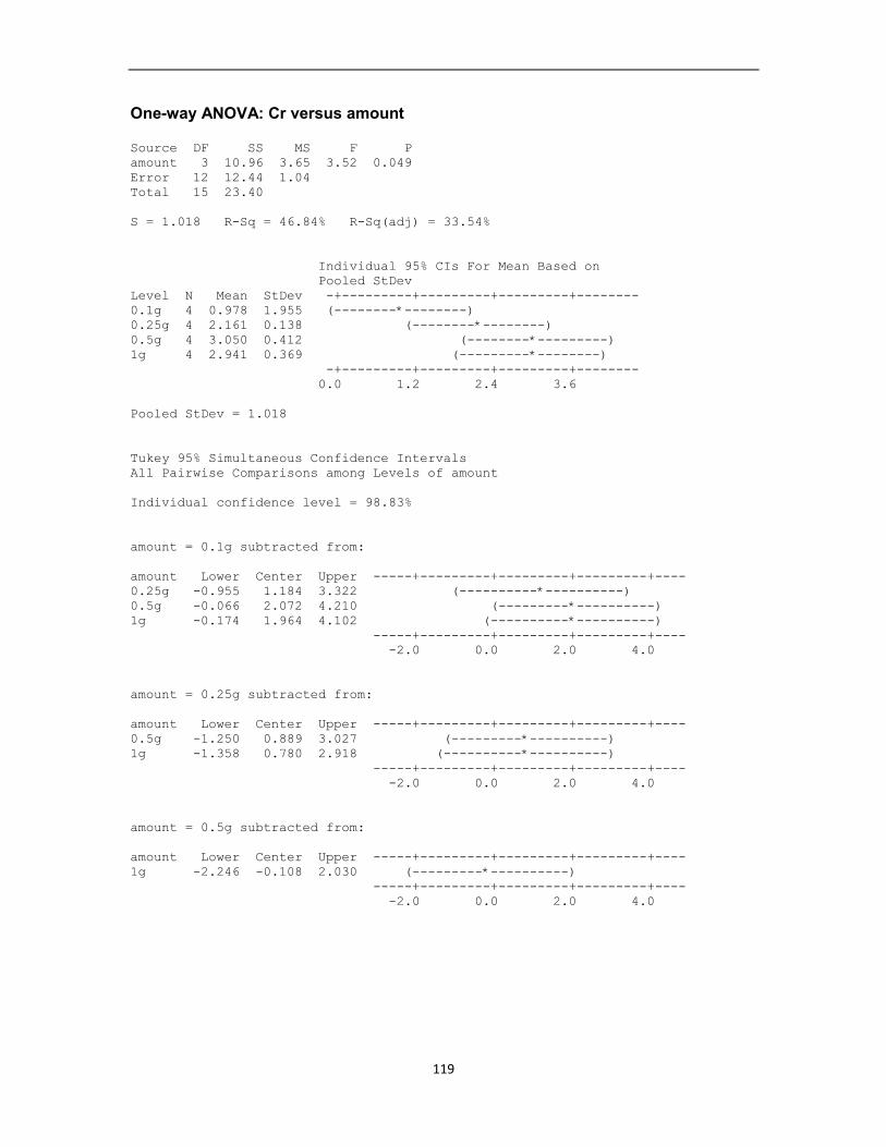
119
One-way ANOVA: Cr versus amount Source DF SS MS F P
amount 3 10.96 3.65 3.52 0.049
Error 12 12.44 1.04
Total 15 23.40
S = 1.018 R-Sq = 46.84% R-Sq(adj) = 33.54%
Individual 95% CIs For Mean Based on
Pooled StDev
Level N Mean StDev -+---------+---------+---------+--------
0.1g 4 0.978 1.955 (--------*--------)
0.25g 4 2.161 0.138 (--------*--------)
0.5g 4 3.050 0.412 (--------*---------)
1g 4 2.941 0.369 (---------*--------)
-+---------+---------+---------+--------
0.0 1.2 2.4 3.6
Pooled StDev = 1.018
Tukey 95% Simultaneous Confidence Intervals
All Pairwise Comparisons among Levels of amount
Individual confidence level = 98.83%
amount = 0.1g subtracted from:
amount Lower Center Upper -----+---------+---------+---------+----
0.25g -0.955 1.184 3.322 (----------*----------)
0.5g -0.066 2.072 4.210 (---------*----------)
1g -0.174 1.964 4.102 (----------*----------)
-----+---------+---------+---------+----
-2.0 0.0 2.0 4.0
amount = 0.25g subtracted from:
amount Lower Center Upper -----+---------+---------+---------+----
0.5g -1.250 0.889 3.027 (---------*----------)
1g -1.358 0.780 2.918 (----------*----------)
-----+---------+---------+---------+----
-2.0 0.0 2.0 4.0
amount = 0.5g subtracted from:
amount Lower Center Upper -----+---------+---------+---------+----
1g -2.246 -0.108 2.030 (---------*----------)
-----+---------+---------+---------+----
-2.0 0.0 2.0 4.0

120
One-way ANOVA: Cu versus amount Source DF SS MS F P
amount 3 25.97 8.66 4.04 0.034
Error 12 25.74 2.14
Total 15 51.71
S = 1.465 R-Sq = 50.22% R-Sq(adj) = 37.78%
Individual 95% CIs For Mean Based on
Pooled StDev
Level N Mean StDev -----+---------+---------+---------+----
0.1g 4 0.816 1.633 (---------*---------)
0.25g 4 1.984 2.296 (---------*---------)
0.5g 4 3.996 0.354 (---------*---------)
1g 4 3.591 0.720 (---------*---------)
-----+---------+---------+---------+----
0.0 1.6 3.2 4.8
Pooled StDev = 1.465
Tukey 95% Simultaneous Confidence Intervals
All Pairwise Comparisons among Levels of amount
Individual confidence level = 98.83%
amount = 0.1g subtracted from:
amount Lower Center Upper -------+---------+---------+---------+--
0.25g -1.908 1.168 4.243 (---------*---------)
0.5g 0.104 3.180 6.255 (----------*---------)
1g -0.300 2.775 5.851 (---------*----------)
-------+---------+---------+---------+--
-3.0 0.0 3.0 6.0
amount = 0.25g subtracted from:
amount Lower Center Upper -------+---------+---------+---------+--
0.5g -1.064 2.012 5.087 (----------*---------)
1g -1.468 1.607 4.683 (---------*----------)
-------+---------+---------+---------+--
-3.0 0.0 3.0 6.0
amount = 0.5g subtracted from:
amount Lower Center Upper -------+---------+---------+---------+--
1g -3.480 -0.404 2.671 (----------*---------)
-------+---------+---------+---------+--
-3.0 0.0 3.0 6.0

121
One-way ANOVA: Mn versus amount Source DF SS MS F P
amount 3 44.39 14.80 10.06 0.001
Error 12 17.65 1.47
Total 15 62.04
S = 1.213 R-Sq = 71.55% R-Sq(adj) = 64.44%
Individual 95% CIs For Mean Based on
Pooled StDev
Level N Mean StDev --+---------+---------+---------+-------
0.1g 4 8.878 1.213 (-----*------)
0.25g 4 9.319 1.544 (------*-----)
0.5g 4 13.060 1.216 (-----*------)
1g 4 11.266 0.741 (-----*------)
--+---------+---------+---------+-------
8.0 10.0 12.0 14.0
Pooled StDev = 1.213
Tukey 95% Simultaneous Confidence Intervals
All Pairwise Comparisons among Levels of amount
Individual confidence level = 98.83%
amount = 0.1g subtracted from:
amount Lower Center Upper --------+---------+---------+---------+-
0.25g -2.106 0.441 2.988 (------*-------)
0.5g 1.635 4.182 6.729 (------*------)
1g -0.158 2.388 4.935 (------*------)
--------+---------+---------+---------+-
-3.5 0.0 3.5 7.0
amount = 0.25g subtracted from:
amount Lower Center Upper --------+---------+---------+---------+-
0.5g 1.194 3.741 6.288 (-------*------)
1g -0.599 1.947 4.494 (-------*------)
--------+---------+---------+---------+-
-3.5 0.0 3.5 7.0
amount = 0.5g subtracted from:
amount Lower Center Upper --------+---------+---------+---------+-
1g -4.340 -1.794 0.753 (------*------)
--------+---------+---------+---------+-
-3.5 0.0 3.5 7.0

122
One-way ANOVA: Ni versus amount Source DF SS MS F P
amount 3 12.079 4.026 9.08 0.002
Error 12 5.322 0.444
Total 15 17.401
S = 0.6660 R-Sq = 69.41% R-Sq(adj) = 61.77%
Individual 95% CIs For Mean Based on
Pooled StDev
Level N Mean StDev +---------+---------+---------+---------
0.1g 4 0.6925 0.8717 (------*------)
0.25g 4 1.9135 0.9364 (------*------)
0.5g 4 3.0203 0.1957 (------*------)
1g 4 2.5165 0.3148 (------*------)
+---------+---------+---------+---------
0.0 1.0 2.0 3.0
Pooled StDev = 0.6660
Tukey 95% Simultaneous Confidence Intervals
All Pairwise Comparisons among Levels of amount
Individual confidence level = 98.83%
amount = 0.1g subtracted from:
amount Lower Center Upper ------+---------+---------+---------+---
0.25g -0.1775 1.2210 2.6195 (--------*-------)
0.5g 0.9292 2.3278 3.7263 (--------*-------)
1g 0.4255 1.8240 3.2225 (-------*--------)
------+---------+---------+---------+---
-1.6 0.0 1.6 3.2
amount = 0.25g subtracted from:
amount Lower Center Upper ------+---------+---------+---------+---
0.5g -0.2918 1.1067 2.5053 (--------*--------)
1g -0.7955 0.6030 2.0015 (--------*--------)
------+---------+---------+---------+---
-1.6 0.0 1.6 3.2
amount = 0.5g subtracted from:
amount Lower Center Upper ------+---------+---------+---------+---
1g -1.9023 -0.5038 0.8948 (--------*--------)
------+---------+---------+---------+---
-1.6 0.0 1.6 3.2

123
One-way ANOVA: Se versus amount Source DF SS MS F P
amount 3 15.294 5.098 12.01 0.001
Error 12 5.096 0.425
Total 15 20.390
S = 0.6517 R-Sq = 75.01% R-Sq(adj) = 68.76%
Individual 95% CIs For Mean Based on
Pooled StDev
Level N Mean StDev ---+---------+---------+---------+------
0.1g 4 0.3973 0.7945 (------*------)
0.25g 4 0.5695 0.8936 (------*------)
0.5g 4 2.5098 0.3917 (------*------)
1g 4 2.3540 0.3398 (-------*------)
---+---------+---------+---------+------
0.0 1.0 2.0 3.0
Pooled StDev = 0.6517
Tukey 95% Simultaneous Confidence Intervals
All Pairwise Comparisons among Levels of amount
Individual confidence level = 98.83%
amount = 0.1g subtracted from:
amount Lower Center Upper -------+---------+---------+---------+--
0.25g -1.1962 0.1722 1.5407 (------*------)
0.5g 0.7440 2.1125 3.4810 (------*-----)
1g 0.5882 1.9567 3.3252 (------*------)
-------+---------+---------+---------+--
-2.0 0.0 2.0 4.0
amount = 0.25g subtracted from:
amount Lower Center Upper -------+---------+---------+---------+--
0.5g 0.5718 1.9403 3.3087 (------*------)
1g 0.4160 1.7845 3.1529 (------*------)
-------+---------+---------+---------+--
-2.0 0.0 2.0 4.0
amount = 0.5g subtracted from:
amount Lower Center Upper -------+---------+---------+---------+--
1g -1.5243 -0.1558 1.2127 (------*------)
-------+---------+---------+---------+--
-2.0 0.0 2.0 4.0

124
One-way ANOVA: Zn versus amount Source DF SS MS F P
amount 3 56.58 18.86 4.90 0.019
Error 12 46.23 3.85
Total 15 102.81
S = 1.963 R-Sq = 55.03% R-Sq(adj) = 43.79%
Individual 95% CIs For Mean Based on Pooled
StDev
Level N Mean StDev +---------+---------+---------+---------
0.1g 4 17.240 2.597 (--------*--------)
0.25g 4 19.602 2.085 (-------*--------)
0.5g 4 21.710 1.711 (--------*-------)
1g 4 21.868 1.179 (-------*--------)
+---------+---------+---------+---------
15.0 17.5 20.0 22.5
Pooled StDev = 1.963
Tukey 95% Simultaneous Confidence Intervals
All Pairwise Comparisons among Levels of amount
Individual confidence level = 98.83%
amount = 0.1g subtracted from:
amount Lower Center Upper ------+---------+---------+---------+---
0.25g -1.760 2.362 6.484 (---------*---------)
0.5g 0.348 4.469 8.591 (---------*---------)
1g 0.506 4.628 8.750 (----------*---------)
------+---------+---------+---------+---
-4.0 0.0 4.0 8.0
amount = 0.25g subtracted from:
amount Lower Center Upper ------+---------+---------+---------+---
0.5g -2.014 2.108 6.230 (---------*----------)
1g -1.855 2.267 6.389 (----------*---------)
------+---------+---------+---------+---
-4.0 0.0 4.0 8.0
amount = 0.5g subtracted from:
amount Lower Center Upper ------+---------+---------+---------+---
1g -3.963 0.159 4.281 (---------*----------)
------+---------+---------+---------+---
-4.0 0.0 4.0 8.0

125
One-way ANOVA: As versus amount
Source DF SS MS F P
amount 3 197.9 66.0 5.09 0.017
Error 12 155.5 13.0
Total 15 353.4
S = 3.600 R-Sq = 56.00% R-Sq(adj) = 45.00%
Individual 95% CIs For Mean Based on
Pooled StDev
Level N Mean StDev ----+---------+---------+---------+-----
0.1g 4 50.980 4.626 (-------*-------)
0.25g 4 47.380 4.471 (-------*-------)
0.5g 4 43.781 3.063 (-------*------)
1g 4 41.775 1.031 (-------*------)
----+---------+---------+---------+-----
40.0 45.0 50.0 55.0
Pooled StDev = 3.600
Tukey 95% Simultaneous Confidence Intervals
All Pairwise Comparisons among Levels of amount
Individual confidence level = 98.83%
amount = 0.1g subtracted from:
amount Lower Center Upper -+---------+---------+---------+--------
0.25g -11.160 -3.601 3.959 (--------*---------)
0.5g -14.759 -7.200 0.360 (--------*--------)
1g -16.764 -9.205 -1.646 (--------*---------)
-+---------+---------+---------+--------
-16.0 -8.0 0.0 8.0
amount = 0.25g subtracted from:
amount Lower Center Upper -+---------+---------+---------+--------
0.5g -11.158 -3.599 3.960 (---------*--------)
1g -13.164 -5.604 1.955 (--------*--------)
-+---------+---------+---------+--------
-16.0 -8.0 0.0 8.0
amount = 0.5g subtracted from:
amount Lower Center Upper -+---------+---------+---------+--------
1g -9.565 -2.005 5.554 (--------*---------)
-+---------+---------+---------+--------
-16.0 -8.0 0.0 8.0

126
One-way ANOVA: Cd versus amount Source DF SS MS F P
amount 3 13.253 4.418 9.37 0.002
Error 12 5.659 0.472
Total 15 18.913
S = 0.6867 R-Sq = 70.08% R-Sq(adj) = 62.59%
Individual 95% CIs For Mean Based on
Pooled StDev
Level N Mean StDev ---+---------+---------+---------+------
0.1g 4 0.4963 0.5847 (-------*------)
0.25g 4 1.0410 1.2021 (------*-------)
0.5g 4 2.7073 0.2269 (------*-------)
1g 4 2.3525 0.2195 (-------*------)
---+---------+---------+---------+------
0.0 1.0 2.0 3.0
Pooled StDev = 0.6867
Tukey 95% Simultaneous Confidence Intervals
All Pairwise Comparisons among Levels of amount
Individual confidence level = 98.83%
amount = 0.1g subtracted from:
amount Lower Center Upper ------+---------+---------+---------+---
0.25g -0.8974 0.5448 1.9869 (------*------)
0.5g 0.7688 2.2110 3.6532 (------*------)
1g 0.4141 1.8563 3.2984 (------*------)
------+---------+---------+---------+---
-2.0 0.0 2.0 4.0
amount = 0.25g subtracted from:
amount Lower Center Upper ------+---------+---------+---------+---
0.5g 0.2241 1.6663 3.1084 (------*-------)
1g -0.1307 1.3115 2.7537 (-------*------)
------+---------+---------+---------+---
-2.0 0.0 2.0 4.0
amount = 0.5g subtracted from:
amount Lower Center Upper ------+---------+---------+---------+---
1g -1.7969 -0.3548 1.0874 (------*------)
------+---------+---------+---------+---
-2.0 0.0 2.0 4.0

127
One-way ANOVA: Hg mg/kg versus amount Source DF SS MS F P
amount 3 0.0003998 0.0001333 3.53 0.049
Error 12 0.0004534 0.0000378
Total 15 0.0008532
S = 0.006147 R-Sq = 46.86% R-Sq(adj) = 33.57%
Individual 95% CIs For Mean Based on Pooled
StDev
Level N Mean StDev +---------+---------+---------+---------
0.1g 4 0.000000 0.000000 (---------*---------)
0.25g 4 0.002500 0.005000 (---------*--------)
0.5g 4 0.009725 0.006912 (---------*--------)
1g 4 0.012153 0.008852 (--------*---------)
+---------+---------+---------+---------
-0.0070 0.0000 0.0070 0.0140
Pooled StDev = 0.006147
Tukey 95% Simultaneous Confidence Intervals
All Pairwise Comparisons among Levels of amount
Individual confidence level = 98.83%
amount = 0.1g subtracted from:
amount Lower Center Upper
0.25g -0.010409 0.002500 0.015409
0.5g -0.003184 0.009725 0.022634
1g -0.000756 0.012153 0.025061
amount ---------+---------+---------+---------+
0.25g (----------*----------)
0.5g (----------*----------)
1g (----------*----------)
---------+---------+---------+---------+
-0.012 0.000 0.012 0.024
amount = 0.25g subtracted from:
amount Lower Center Upper
0.5g -0.005684 0.007225 0.020134
1g -0.003256 0.009653 0.022561
amount ---------+---------+---------+---------+
0.5g (----------*----------)
1g (----------*----------)
---------+---------+---------+---------+
-0.012 0.000 0.012 0.024
amount = 0.5g subtracted from:
amount Lower Center Upper
1g -0.010481 0.002428 0.015336
amount ---------+---------+---------+---------+
1g (----------*----------)
---------+---------+---------+---------+
-0.012 0.000 0.012 0.024

128
One-way ANOVA: Pb versus amount Source DF SS MS F P
amount 3 7.283 2.428 9.71 0.002
Error 12 3.000 0.250
Total 15 10.283
S = 0.5000 R-Sq = 70.83% R-Sq(adj) = 63.53%
Individual 95% CIs For Mean Based on
Pooled StDev
Level N Mean StDev -------+---------+---------+---------+--
0.1g 4 0.7475 0.8742 (-----*------)
0.25g 4 1.8495 0.4534 (------*------)
0.5g 4 2.4640 0.1313 (------*------)
1g 4 2.3278 0.1137 (------*------)
-------+---------+---------+---------+--
0.80 1.60 2.40 3.20
Pooled StDev = 0.5000
Tukey 95% Simultaneous Confidence Intervals
All Pairwise Comparisons among Levels of amount
Individual confidence level = 98.83%
amount = 0.1g subtracted from:
amount Lower Center Upper ----+---------+---------+---------+-----
0.25g 0.0520 1.1020 2.1520 (--------*--------)
0.5g 0.6665 1.7165 2.7665 (-------*--------)
1g 0.5303 1.5803 2.6302 (--------*--------)
----+---------+---------+---------+-----
-1.2 0.0 1.2 2.4
amount = 0.25g subtracted from:
amount Lower Center Upper ----+---------+---------+---------+-----
0.5g -0.4355 0.6145 1.6645 (--------*--------)
1g -0.5717 0.4783 1.5282 (--------*--------)
----+---------+---------+---------+-----
-1.2 0.0 1.2 2.4
amount = 0.5g subtracted from:
amount Lower Center Upper ----+---------+---------+---------+-----
1g -1.1863 -0.1363 0.9137 (--------*--------)
----+---------+---------+---------+-----
-1.2 0.0 1.2 2.4

129
Appendix 2: Statistical outputs for the comparison of freeze dried
versus oven dried samples
(Ca) Paired T-Test and CI: oven dry, freeze dry Paired T for oven dry - freeze dry
N Mean StDev SE Mean
oven dry 6 8.73597 0.19801 0.08084
freeze dry 6 8.59121 0.26967 0.11009
Difference 6 0.144757 0.347025 0.141672
95% CI for mean difference: (-0.219424, 0.508937)
T-Test of mean difference = 0 (vs not = 0): T-Value = 1.02 P-Value = 0.354
(K) Paired T-Test and CI: oven dry, freeze dry Paired T for oven dry - freeze dry
N Mean StDev SE Mean
oven dry 6 30.3135 0.3498 0.1428
freeze dry 6 29.7071 0.7956 0.3248
Difference 6 0.606393 0.782443 0.319431
95% CI for mean difference: (-0.214730, 1.427516)
T-Test of mean difference = 0 (vs not = 0): T-Value = 1.90 P-Value = 0.116
(Mg) Paired T-Test and CI: oven dry, freeze dry Paired T for oven dry - freeze dry
N Mean StDev SE Mean
oven dry 6 8.51619 0.15767 0.06437
freeze dry 6 8.49138 0.27662 0.11293
Difference 6 0.024803 0.269298 0.109940
95% CI for mean difference: (-0.257807, 0.307414)
T-Test of mean difference = 0 (vs not = 0): T-Value = 0.23 P-Value = 0.830
(Na) Paired T-Test and CI: oven dry, freeze dry Paired T for oven dry - freeze dry
N Mean StDev SE Mean
oven dry 6 24.4314 0.7267 0.2967
freeze dry 6 24.1623 0.4860 0.1984
Difference 6 0.269087 0.799757 0.326499
95% CI for mean difference: (-0.570206, 1.108381)
T-Test of mean difference = 0 (vs not = 0): T-Value = 0.82 P-Value = 0.447
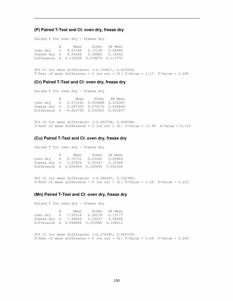
130
(P) Paired T-Test and CI: oven dry, freeze dry Paired T for oven dry - freeze dry
N Mean StDev SE Mean
oven dry 6 8.67344 0.17136 0.06996
freeze dry 6 8.54040 0.34882 0.14240
Difference 6 0.133038 0.278679 0.113770
95% CI for mean difference: (-0.159417, 0.425494)
T-Test of mean difference = 0 (vs not = 0): T-Value = 1.17 P-Value = 0.295
(Cr) Paired T-Test and CI: oven dry, freeze dry Paired T for oven dry - freeze dry
N Mean StDev SE Mean
oven dry 6 0.571591 0.059688 0.024367
freeze dry 6 0.597320 0.070175 0.028649
Difference 6 -0.025730 0.032425 0.013237
95% CI for mean difference: (-0.059758, 0.008298)
T-Test of mean difference = 0 (vs not = 0): T-Value = -1.94 P-Value = 0.110
(Cu) Paired T-Test and CI: oven dry, freeze dry Paired T for oven dry - freeze dry
N Mean StDev SE Mean
oven dry 6 2.72751 0.23183 0.09464
freeze dry 6 2.67054 0.25347 0.10348
Difference 6 0.056969 0.100450 0.041009
95% CI for mean difference: (-0.048447, 0.162385)
T-Test of mean difference = 0 (vs not = 0): T-Value = 1.39 P-Value = 0.223
(Mn) Paired T-Test and CI: oven dry, freeze dry Paired T for oven dry - freeze dry
N Mean StDev SE Mean
oven dry 6 7.55316 0.32278 0.13177
freeze dry 6 7.45826 0.23257 0.09495
Difference 6 0.094896 0.353980 0.144512
95% CI for mean difference: (-0.276583, 0.466376)
T-Test of mean difference = 0 (vs not = 0): T-Value = 0.66 P-Value = 0.540

131
(Ni) Paired T-Test and CI: oven dry, freeze dry Paired T for oven dry - freeze dry
N Mean StDev SE Mean
oven dry 6 2.17741 0.20342 0.08305
freeze dry 6 1.87468 0.42105 0.17189
Difference 6 0.302728 0.570458 0.232888
95% CI for mean difference: (-0.295931, 0.901386)
T-Test of mean difference = 0 (vs not = 0): T-Value = 1.30 P-Value = 0.250
(Se) Paired T-Test and CI: oven dry, freeze dry Paired T for oven dry - freeze dry
N Mean StDev SE Mean
oven dry 6 0.802939 0.047353 0.019332
freeze dry 6 0.798272 0.056416 0.023032
Difference 6 0.004667 0.080653 0.032926
95% CI for mean difference: (-0.079973, 0.089307)
T-Test of mean difference = 0 (vs not = 0): T-Value = 0.14 P-Value = 0.893
(Zn) Paired T-Test and CI: oven dry, freeze dry Paired T for oven dry - freeze dry
N Mean StDev SE Mean
oven dry 6 30.2543 0.7433 0.3035
freeze dry 6 30.1419 2.1486 0.8772
Difference 6 0.112435 2.278551 0.930215
95% CI for mean difference: (-2.278757, 2.503628)
T-Test of mean difference = 0 (vs not = 0): T-Value = 0.12 P-Value = 0.909
(As) Paired T-Test and CI: oven dry, freeze dry Paired T for oven dry - freeze dry
N Mean StDev SE Mean
oven dry 6 33.4294 3.5358 1.4435
freeze dry 6 33.2011 3.5007 1.4292
Difference 6 0.228259 5.361765 2.188931
95% CI for mean difference: (-5.398568, 5.855086)
T-Test of mean difference = 0 (vs not = 0): T-Value = 0.10 P-Value = 0.921

132
(Cd) Paired T-Test and CI: oven dry, freeze dry Paired T for oven dry - freeze dry
N Mean StDev SE Mean
oven dry 6 1.77880 0.14469 0.05907
freeze dry 6 1.78947 0.16042 0.06549
Difference 6 -0.010668 0.075704 0.030906
95% CI for mean difference: (-0.090115, 0.068778)
T-Test of mean difference = 0 (vs not = 0): T-Value = -0.35 P-Value = 0.744
(Hg) Paired T-Test and CI: oven dry, freeze dry Paired T for oven dry - freeze dry
N Mean StDev SE Mean
oven dry 6 0.046758 0.040513 0.016539
freeze dry 6 0.037418 0.042865 0.017499
Difference 6 0.009340 0.042839 0.017489
95% CI for mean difference: (-0.035617, 0.054296)
T-Test of mean difference = 0 (vs not = 0): T-Value = 0.53 P-Value = 0.616
(Pb) Paired T-Test and CI: oven dry, freeze dry Paired T for oven dry - freeze dry
N Mean StDev SE Mean
oven dry 6 0.267955 0.026664 0.010886
freeze dry 6 0.247316 0.019874 0.008113
Difference 6 0.020639 0.022149 0.009042
95% CI for mean difference: (-0.002604, 0.043883)
T-Test of mean difference = 0 (vs not = 0): T-Value = 2.28 P-Value = 0.071

133
Appendix 3: Table of metal contents of Undaria pinnatifida collected
from four different sites in New Zealand.
Values are the range of the monthly means ± standard error
Metal Site Blade Sporophyll
Ca (g/kg) PE327 9.77 ± 0.148(April) – 16.97
± 0.45 (June)
7.88 ± 0.24(April) – 8.75 ±
0.35(June)
Ca (g/kg) 106 8.26 ± 0.08 (August) –
9.07 ± 0.34 (October)
6.37 ± 0.13(July) – 7.03 ±
0.39(October)
Ca (g/kg) Wellington Site
A
8.89 ± 0.17(August) –
10.13 ± 0.20 (October)
6.72 ± 0.17(August) – 7.03 ±
0.055(October)
Ca (g/kg) Wellington Site
B
8.76 ± 0.20 (August) –
10.31 ± 0.40(October
7.20 ± 0.39(August) – 7.41 ±
0.23(October)
K (g/mg) PE327 19.42 ± 0.26 (May) – 45.86
± 0.91 (October
27.25 ± 0.27(May) – 28.69 ±
0.86(June)
K (g/mg) 106 32.85 ± 0.33 (August) –
42.14 ± 0.59 (October)
15.18 ± 0.54(July) – 16.10 ±
0.44(October)
K (g/mg) Wellington Site
A
29.49 ± 0.62(August) –
44.68 ± 0.52(October)
27.12 ± 0.88(July) – 28.97 ±
0.29(October)
K (g/mg) Wellington Site
B
27.92 ± 0.62(August) –
48.48 ± 0.56(October)
26.21 ± 0.49(November) –
27.08 ± 0.52(October)
Mg (g/kg) PE327 6.83 ± 0.14 (April) – 9.21
± 0.36 (October)
4.58 ± 0.36(April) – 6.64 ±
0.32(October)
Mg (g/kg) 106 8.20 ± 0.16(July) – 9.47 ±
0.31(October)
5.75 ± 0.045(August) – 6.16
± 0.37(October)
Mg (g/kg) Wellington Site
A
8.34 ± 0.32(August) – 9.23
± 0.33(October)
5.45 ± 0.14(November) –
5.72 ± 0.11(August)
Mg (g/kg) Wellington Site
B
8.26 ± 0.21(August)– 9.47
± 0.22(October)
7.30 ± 0.22(August) – 7.59 ±
0.14(October)
Na (g/mg) PE327 11.26 ± 0.19(April) – 62.55
± 0.68(October)
10.46 ± 0.21(April) – 32.10
± 0.46(July)
Na (g/mg) 106 54.24 ± 0.48(August) –
58.31 ± 0.55(October)
30.62 ± 0.47(August) –
33.83 ± 0.50(October)
Na (g/mg) Wellington Site
A
24.83 ± 0.33(August) –
28.60 ± 0.51(October)
10.45 ± 0.14(August) –
20.42 ± 0.16(September)
Na (g/mg) Wellington Site
B
24.15 ± 0.95(August)–
28.18 ± 0.28(October)
9.82 ± 0.35(August) – 19.95
± 0.15(October)
P (g/kg) PE327 9.28 ± 0.19(July) – 12.05 ±
0.23(October
7.89 ± 0.16(May) – 9.41 ±
0.30(October)
P (g/kg) 106 10.41 ± 0.19(July) – 11.62
± 0.26(October)
6.60 ± 0.42(July) – 7.76 ±
0.73(October)
P (g/kg) Wellington Site
A
9.09 ± 0.19(August) –
10.31 ± 0.66(October)
8.24 ± 0.053(November) –
8.54 ± 0.13(October)
P (g/kg) Wellington Site
B
8.60 ± 0.43(August) –
10.61 ± 0.43(October)
7.99 ± 0.16(August) – 8.71 ±
0.11(October)

134
Cr (mg/kg) PE327 0.69 ± 0.094(April) – 1.04
± 0.21(October)
0.76 ± 0.065(April) – 0.92 ±
0.024(June)
Cr (mg/kg) 106 0.74 ± 0.077(August) –
0.78 ± 0.053(July)
0.70 ± 0.027(September) –
0.77 ± 0.016(July)
Cr (mg/kg) Wellington Site
A
0.80 ± 0.093(September) –
0.84 ± 0.020(October)
0.68 ± 0.031(August) – 0.74
± 0.026(October)
Cr (mg/kg) Wellington Site
B
0.64 ± 0.060(August) –
0.73 ± 0.029(October)
0.57 ± 0.06(November) –
0.69 ± 0.019(October)
Cu (mg/kg) PE327 3.08 ± 0.16(July) – 3.78 ±
0.23(October)
1.64 ± 0.16(September) –
1.85 ± 0.11(July)
Cu (mg/kg) 106 2.97 ± 0.22(July) – 3.77 ±
0.23(October)
1.84 ± 0.092(August) – 2.44
± 0.16(October)
Cu (mg/kg) Wellington Site
A
2.28 ± 0.21(August) – 2.62
± 0.15(October)
2.21 ± 0.10(August) – 2.40 ±
0.12(October)
Cu (mg/kg) Wellington Site
B
2.48 ± 0.27(September) –
2.66 ± 0.12(October)
2.33 ± 0.091(September) –
2.64 ± 0.11(October)
Mn (mg/kg) PE327 8.73 ± 0.58(July) – 10.39 ±
2.45(October)
4.79 ± 0.26(July) – 7.72 ±
0.85(April)
Mn (mg/kg) 106 8.25 ± 0.67(August) – 9.99
± 1.26(October)
5.59 ± 0.38(July) – 6.26 ±
0.40(October)
Mn (mg/kg) Wellington Site
A
12.57 ± 0.78(September)–
14.61 ± 1.23(October)
6.86 ± 0.59(November) –
7.68 ± 0.24(October)
Mn (mg/kg) Wellington Site
B
8.36 ± 0.17(November)–
8.57 ± 0.19(October)
7.46 ± 0.28(November) -7.93
± 0.13(October)
Ni (mg/kg) PE327 1.54 ± 0.39(April) – 2.78 ±
0.12(October)
1.14 ± 0.16(May) – 1.62 ±
0.35(April)
Ni (mg/kg) 106 1.81 ± 0.13(July) – 2.24 ±
0.12(October)
1.36 ± 0.045(August) – 1.62
± 0.18(October)
Ni (mg/kg) Wellington Site
A
1.78 ± 0.11(November) –
1.95 ± 0.067(October)
1.50 ± 0.078(November) –
1.69 ± 0.056(August)
Ni (mg/kg) Wellington Site
B
1.91 ± 0.12(August) – 2.10
± 0.057(October)
1.53 ± 0.27(November) –
1.70 ± 0.050(October)
Se (mg/kg) PE327 0.54 ± 0.017(April) – 0.61
± 0.016(October)
0.18 ± 0.0173(June) – 0.33 ±
0.030(July)
Se (mg/kg) 106 0.40 ± 0.02(July) – 0.53 ±
0.056(October)
0.37 ± 0.041(September) –
0.40 ± 0.021(October)
Se (mg/kg) Wellington Site
A
0.80 ± 0.049(September) –
0.83 ± 0.14(August)
0.48 ± 0.039(November) –
0.52 ± 0.03(September)
Se (mg/kg) Wellington Site
B
0.65 ± 0.11(August) – 0.81
± 0.078(October)
0.38 ± 0.03(August) – 0.48 ±
0.025(October)
Zn (mg/kg) PE327 20.52 ± (May) – 26.11 ±
2.71(October)
14.18 ± 1.28(May) – 18.60 ±
0.92(October)
Zn (mg/kg) 106 22.60 ± 0.76(July) – 27.30
± 2.78(October)
21.16 ± 1.70(August) –
23.60 ± 2.33(October)
Zn (mg/kg) Wellington Site
A
30.24 ± 1.64(September) –
33.39 ± 3.99(October)
13.70 ± 1.06(August) –
15.41 ± 0.53(October)
Zn (mg/kg) Wellington Site
B
29.41 ± 1.66(September) –
35.03 ± 2.05(October)
15.10 ± 1.03(November) –
16.01 ± 0.49(October)

135
As (mg/kg) PE327 40.54 ± 2.00(October) -
46.71 ± 0.75(May)
23.84 ± 1.49(April) – 29.47
± 1.75(July)
As (mg/kg) 106 30.41 ± 1.52(August) –
31.89 ± 2.22(July)
23.94 ± 1.45(August) - 29.23
± 2.27(July)
As (mg/kg) Wellington Site
A
34.79 ± 2.25(November) –
42.88 ± 2.56(August)
28.46 ± 5.87(October) –
32.84 ± 2.30(August)
As (mg/kg) Wellington Site
B
32.12 ± 1.77(November) –
36.41 ± 3.30(August)
30.03 ± 2.40(August) –
31.27 ± 7.38(September)
Cd (mg/kg) PE327 2.33 ± 0.21(October) –
2.91 ± 0.097(June)
1.82 ± 0.26(October) – 2.19
± 0.17(May)
Cd (mg/kg) 106 1.57 ± 0.088(August) –
1.74 ± 0.19(October)
1.51 ± 0.059(August) – 1.68
± 0.11(July)
Cd (mg/kg) Wellington Site
A
2.11 ± 0.13(September) –
2.24 ± 0.17(August)
1.97 ± 0.21(October) – 2.10
± 0.17(August)
Cd (mg/kg) Wellington Site
B
1.82 ± 0.29(November) –
2.21 ± 0.21(August)
1.67 ± 0.32(October) – 2.20
± 0.4(September)
Hg (mg/kg) PE327 0.023 ± 0.015(May) –
0.040 ± 0.017(September)
No values
Hg (mg/kg) 106 0.024 ± 0.0086(July) –
0.040 ± 0.0026(September)
No values
Hg (mg/kg) Wellington Site
A
0.021 ± 0.010(August) –
0.042 ± 0.020(November)
No values
Hg (mg/kg) Wellington Site
B
0.021 ± 0.0034(August) –
0.037 ± 0.026(November
No values
Pb (mg/kg) PE327 0.22 ± 0.024(October) –
0.29 ± 0.044(April)
0.14 ± 0.0047(April) – 0.29
± 0.048(May)
Pb (mg/kg) 106 0.24 ± 0.022(October) –
0.30 ± 0.019(July)
0.21 ± 0.015(October) – 0.27
± 0.017(July)
Pb (mg/kg) Wellington Site
A
0.28 ± 0.018(September) –
0.31 ± 0.022(August)
0.23 ± 0.026(October) – 0.25
± 0.016(September)
Pb (mg/kg) Wellington Site
B
0.25 ± 0.032(November) –
0.29 ± 0.029(September)
0.167 ± 0.021(October) –
0.174 ± 0.0167(August)