meta-analysis of wetland values: modeling spatial dependencies randall s. rosenberger oregon state...
TRANSCRIPT
Meta-Analysis of Wetland Values:
Modeling Spatial Dependencies
Randall S. RosenbergerOregon State University
Meidan Bu
Microsoft

Overview Spatial relationships in metadata
Spatial econometric modeling
Application to wetland valuation studies in North America
Sensitivity analysis to intra-study dependence
Conclusions

Research questions Are wetland values correlated across space?
What is the spatial relationship of wetland welfare estimates? geographic closeness ecological linkages socio-economic characteristics of local people
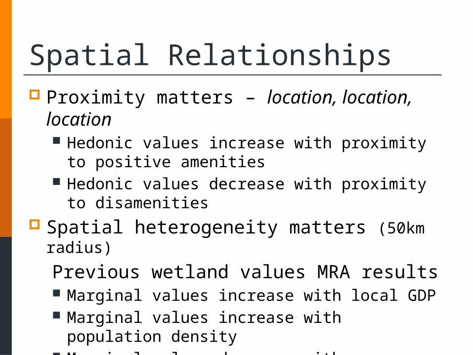
Spatial Relationships Proximity matters – location, location, location
Hedonic values increase with proximity to positive amenities
Hedonic values decrease with proximity to disamenities Spatial heterogeneity matters (50km radius)
Previous wetland values MRA results Marginal values increase with local GDP Marginal values increase with population density Marginal values decrease with resource density
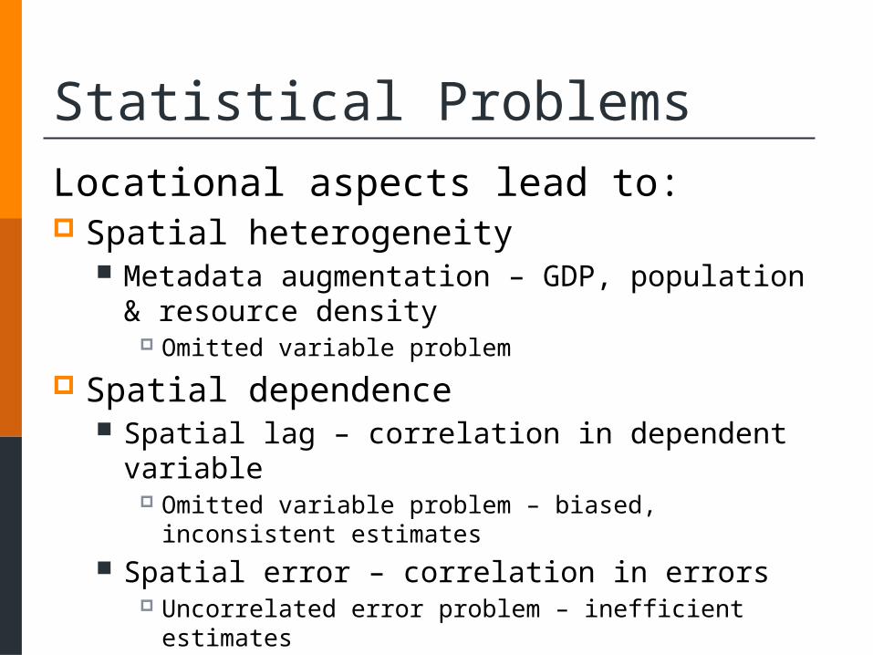
Statistical Problems
Locational aspects lead to: Spatial heterogeneity
Metadata augmentation – GDP, population & resource density
Omitted variable problem
Spatial dependence Spatial lag – correlation in dependent variable
Omitted variable problem – biased, inconsistent estimates Spatial error – correlation in errors
Uncorrelated error problem – inefficient estimates
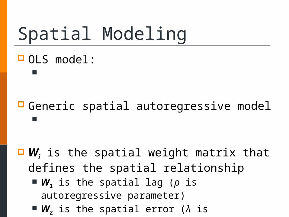
Spatial Modeling OLS model:
Generic spatial autoregressive model
Wi is the spatial weight matrix that defines the spatial relationship W1 is the spatial lag (ρ is autoregressive parameter)
W2 is the spatial error (λ is autoregressive parameter)

The Empirical Model A spatial lag autoregressive model
– standardized wetland welfare estimates from primary studies (per hectare per year in 2010 USD)
- the explanatory variables - the spatial lag (or spatial autoregressive) parameter
– the weight matrix, which defines the spatial neighborhood relationship of wetland sites
(I – ρW)-1 – the spatial multiplier

Spatial Weight Matrix Definition Define an NxN spatial weight matrix C Each element cij reflects spatial influence of location
j on location i
Main diagonal = 0 (i.e., i ≠ j) C is row standardized into W
where i ≠ j
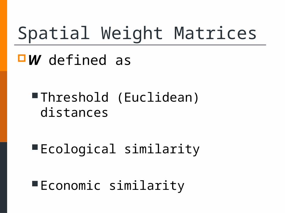
Spatial Weight MatricesW defined as
Threshold (Euclidean) distances
Ecological similarity
Economic similarity
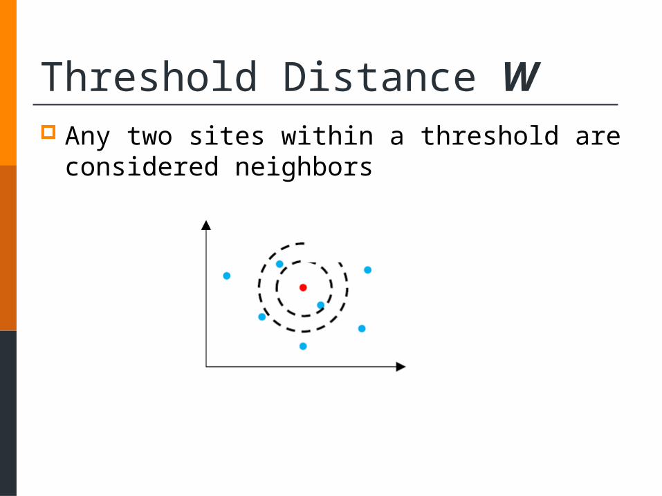
Threshold Distance W Any two sites within a threshold are considered
neighbors
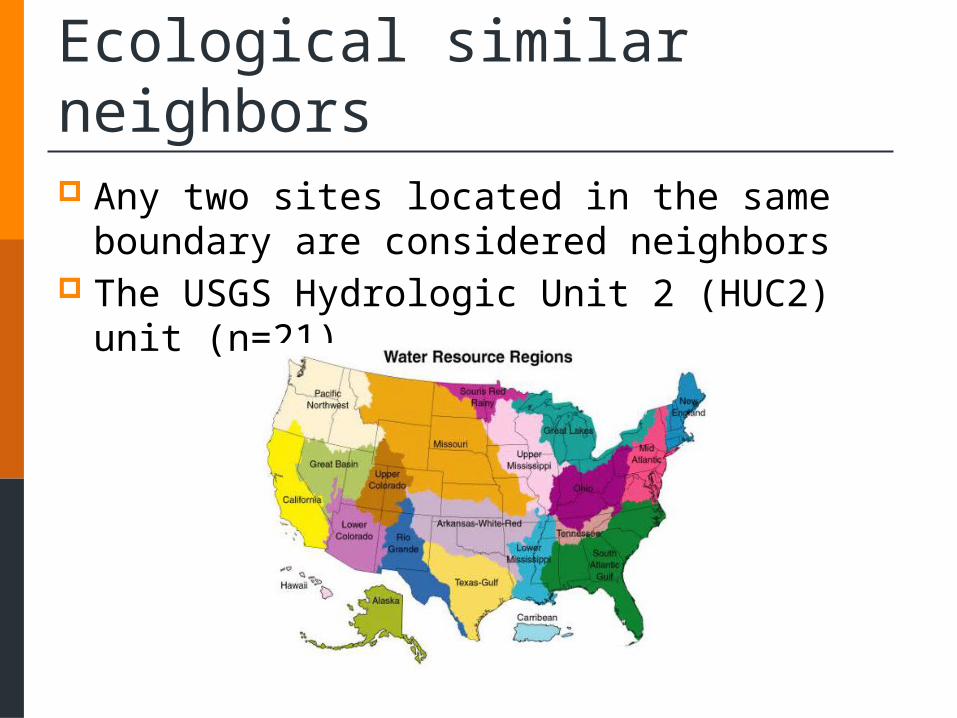
Ecological similar neighbors Any two sites located in the same boundary are
considered neighbors The USGS Hydrologic Unit 2 (HUC2) unit (n=21)

Economic similar neighbors Any two sites sharing the same socioeconomic
attributes (i.e., latent demand) are considered neighbors local education level population density within 50km radius county level average personal income local GDP
Multivariate hierarchical clustering analysis local education level Group observations into clusters (n=40) that have similar
values of measured variables
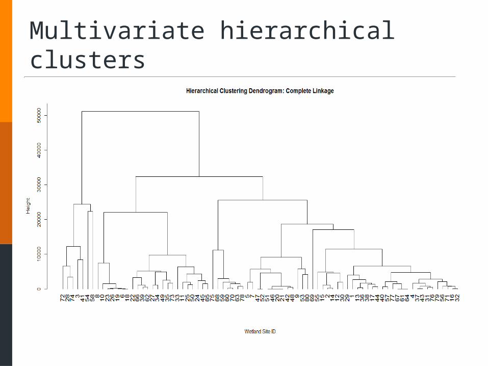
Multivariate hierarchical clusters
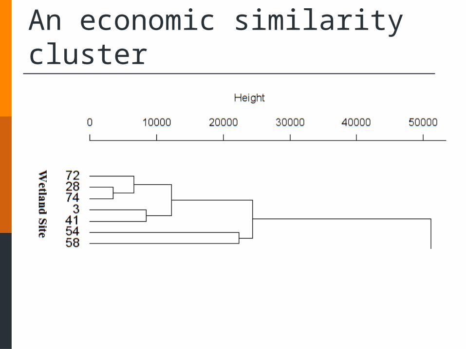
An economic similarity cluster
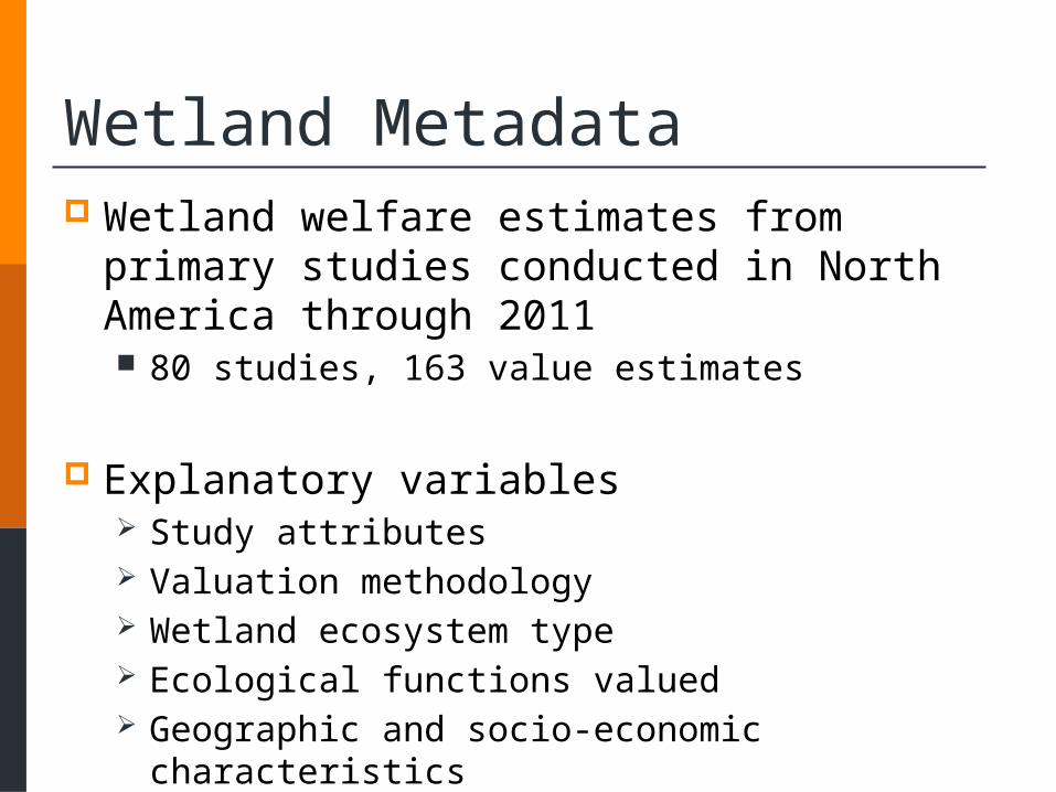
Wetland Metadata Wetland welfare estimates from primary studies
conducted in North America through 2011 80 studies, 163 value estimates
Explanatory variables Study attributes Valuation methodology Wetland ecosystem type Ecological functions valued Geographic and socio-economic characteristics
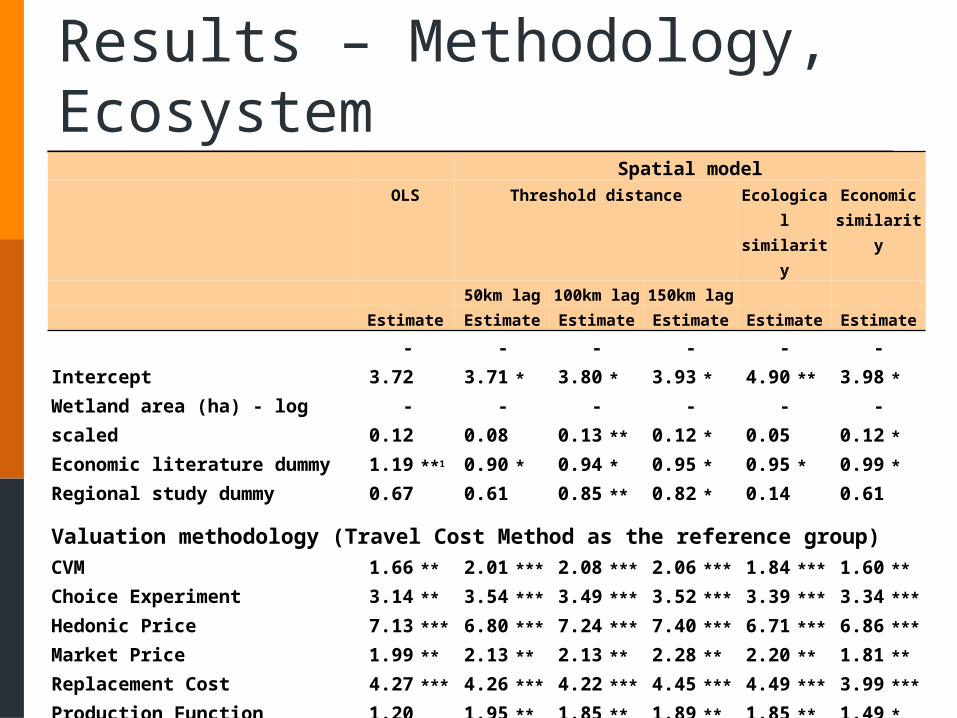
Results – Methodology, EcosystemSpatial model
OLS Threshold distance Ecological similarity
Economic similarity
50km lag 100km lag 150km lagEstimate Estimate Estimate Estimate Estimate Estimate
Intercept -3.72 -3.71 * -3.80 * -3.93 * -4.90 ** -3.98 *
Wetland area (ha) - log scaled -0.12 -0.08 -0.13 ** -0.12 * -0.05 -0.12 *
Economic literature dummy 1.19 **1 0.90 * 0.94 * 0.95 * 0.95 * 0.99 *
Regional study dummy 0.67 0.61 0.85 ** 0.82 * 0.14 0.61
Valuation methodology (Travel Cost Method as the reference group)CVM 1.66 ** 2.01 *** 2.08 *** 2.06 *** 1.84 *** 1.60 **
Choice Experiment 3.14 ** 3.54 *** 3.49 *** 3.52 *** 3.39 *** 3.34 ***
Hedonic Price 7.13 *** 6.80 *** 7.24 *** 7.40 *** 6.71 *** 6.86 ***
Market Price 1.99 ** 2.13 ** 2.13 ** 2.28 ** 2.20 ** 1.81 **
Replacement Cost 4.27 *** 4.26 *** 4.22 *** 4.45 *** 4.49 *** 3.99 ***
Production Function 1.20 1.95 ** 1.85 ** 1.89 ** 1.85 ** 1.49 *
Wetland ecosystem type (Estuarine as the reference group)Riverine 2.00 ** 1.00 1.75 ** 1.82 ** 1.81 ** 1.62 **
Palustrine 0.50 0.39 0.57 0.60 0.76 0.55Lacustrine 0.94 0.88 1.09 * 0.95 0.82 0.91
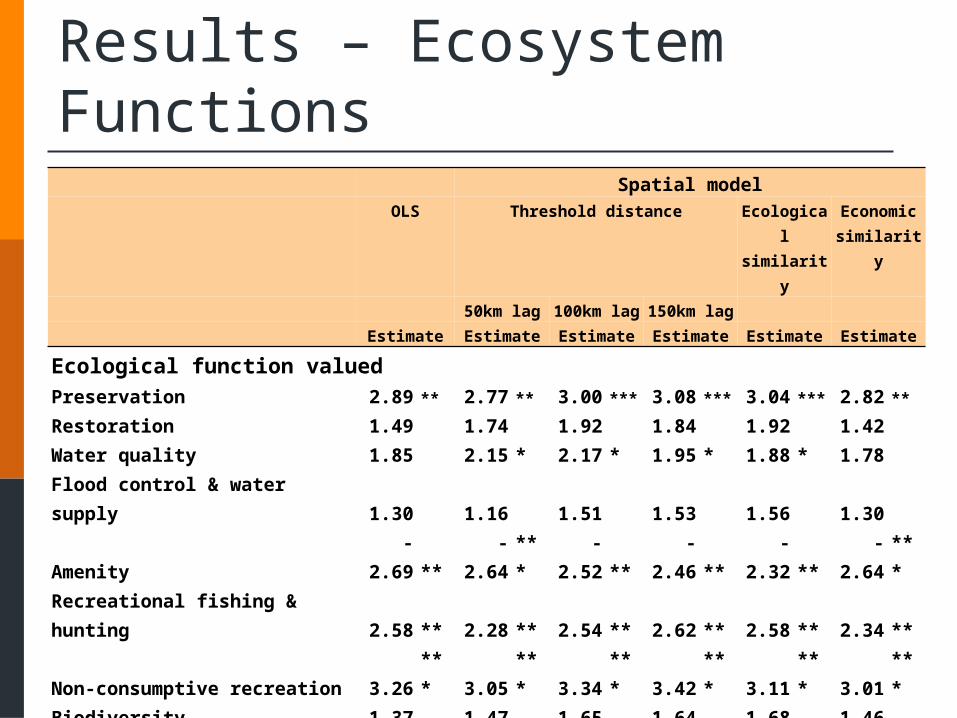
Results – Ecosystem FunctionsSpatial model
OLS Threshold distance Ecological similarity
Economic similarity
50km lag 100km lag 150km lagEstimate Estimate Estimate Estimate Estimate Estimate
Ecological function valuedPreservation 2.89 ** 2.77 ** 3.00 *** 3.08 *** 3.04 *** 2.82 **
Restoration 1.49 1.74 1.92 1.84 1.92 1.42Water quality 1.85 2.15 * 2.17 * 1.95 * 1.88 * 1.78Flood control & water supply 1.30 1.16 1.51 1.53 1.56 1.30Amenity -2.69 ** -2.64 *** -2.52 ** -2.46 ** -2.32 ** -2.64 ***Recreational fishing & hunting 2.58 ** 2.28 ** 2.54 ** 2.62 ** 2.58 ** 2.34 **Non-consumptive recreation 3.26 *** 3.05 *** 3.34 *** 3.42 *** 3.11 *** 3.01 ***Biodiversity 1.37 1.47 1.65 1.64 1.68 1.46Commercial fishing & hunting 1.47 1.04 1.48 1.47 1.53 1.28
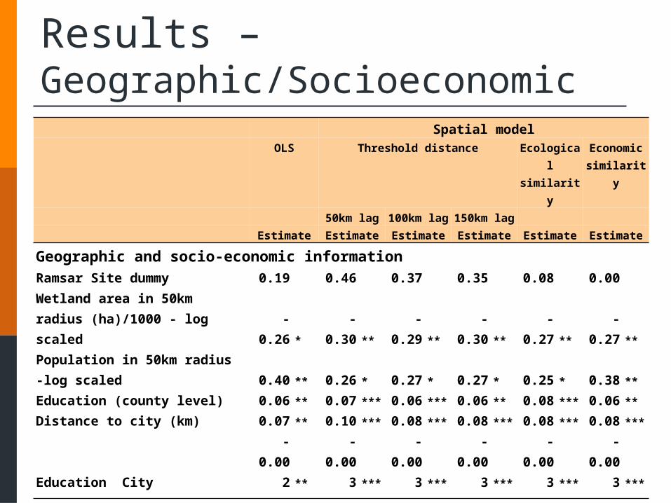
Results – Geographic/SocioeconomicSpatial model
OLS Threshold distance Ecological similarity
Economic similarity
50km lag 100km lag 150km lagEstimate Estimate Estimate Estimate Estimate Estimate
Geographic and socio-economic informationRamsar Site dummy 0.19 0.46 0.37 0.35 0.08 0.00Wetland area in 50km radius (ha)/1000 - log scaled -0.26 * -0.30 ** -0.29 ** -0.30 ** -0.27 ** -0.27 **
Population in 50km radius -log scaled 0.40 ** 0.26 * 0.27 * 0.27 * 0.25 * 0.38 **
Education (county level) 0.06 ** 0.07 *** 0.06 *** 0.06 ** 0.08 *** 0.06 **
Distance to city (km) 0.07 ** 0.10 *** 0.08 *** 0.08 *** 0.08 *** 0.08 ***
Education City -0.002 ** -0.003 *** -0.003 *** -0.003 *** -0.003 *** -0.003 ***

Results – Test StatisticsSpatial model
OLS Threshold distance Ecological similarity
Economic similarity
50km lag 100km lag 150km lag
Estimate Estimate Estimate Estimate Estimate Estimate
N 163 163 163 163 163 163R2 0.50
(spatial autoregressive parameter) 0.176 0.143 0.138 0.179 0.095Likelihood ratio test statistic 17 10 9 9 4P-value for the likelihood ratio test <0.000 *** 0.001 *** 0.003 *** 0.003 *** 0.036 **
AIC 726 710 717 718 719 723

Recap – Spatial MRAs Positive spatial correlation for all three neighborhood
criteria Threshold distance neighbors are strongest
correlation Spatial correlation exists as far as 150km
Economic similarity defined neighbors has the weakest correlation
Covariate estimates are robust to spatial dependence, although magnitude varies some

Intra-study Correlation
What about confounding intra-study correlation?
An unbalanced panel meta-dataset with 163 observations from 80 wetland sites 39 wetland sites report multiple measures (max = 16 obs.)

Bootstrap Sensitivity Analysis Bootstrap draw one observation per wetland site
Form 1000 sub-datasets
Repeat spatial MRAs
Test the significance of spatial correlation for every combination
Count the number of significant LLR results
Test the robustness of the spatial correlation
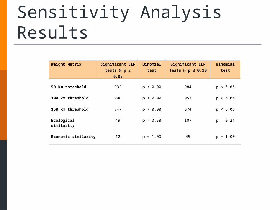
Sensitivity Analysis Results
Weight Matrix Significant LLR tests @ p ≤
0.05
Binomial test
Significant LLR tests @ p ≤ 0.10
Binomial test
50 km threshold 933 p < 0.00 984 p < 0.00
100 km threshold 908 p < 0.00 957 p < 0.00
150 km threshold 747 p < 0.00 874 p < 0.00
Ecological similarity 49 p = 0.58 107 p = 0.24
Economic similarity 12 p = 1.00 45 p = 1.00
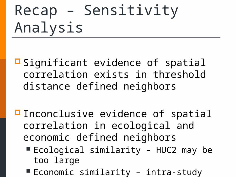
Recap – Sensitivity Analysis
Significant evidence of spatial correlation exists in threshold distance defined neighbors
Inconclusive evidence of spatial correlation in ecological and economic defined neighbors Ecological similarity – HUC2 may be too large Economic similarity – intra-study correlation

Conclusions Spatial correlation exists, although partial effects are
robust to specifications
Threshold distance is robust to intra-study correlation
Future issues: Other spatial models (e.g., spatial error specification)? What are the implications for international benefit transfers? Are results consistent for other spatially dependent
metadata?

Q&A
We hope you enjoyed this tour of spatial econometric modeling in an MRA framework
THANK YOU!

The Parking Lot - Descriptives
Mean St. Dev. Min Max
Wetland welfare estimate/ha/year in 2010 USD –log scaled
5.85
2.65
-1.50
11.81
Wetland area (ha) - log scaled 8.46 4.02 0.05 16.73
Economic literature dummy 0.63 0.48 0 1
Regional study dummy 0.42 0.50 0 1

The Parking Lot - Descriptives
Mean St. Dev. Min Max Valuation methodology (binary variables)
CVM 0.24 0.43 0 1
Choice Experiment 0.04 0.19 0 1
Travel Cost 0.19 0.39 0 1
Hedonic Price 0.05 0.22 0 1
Market Price 0.28 0.45 0 1
Replacement Cost 0.09 0.28 0 1
Production Function 0.12 0.33 0 1
The Parking Lot - Descriptives
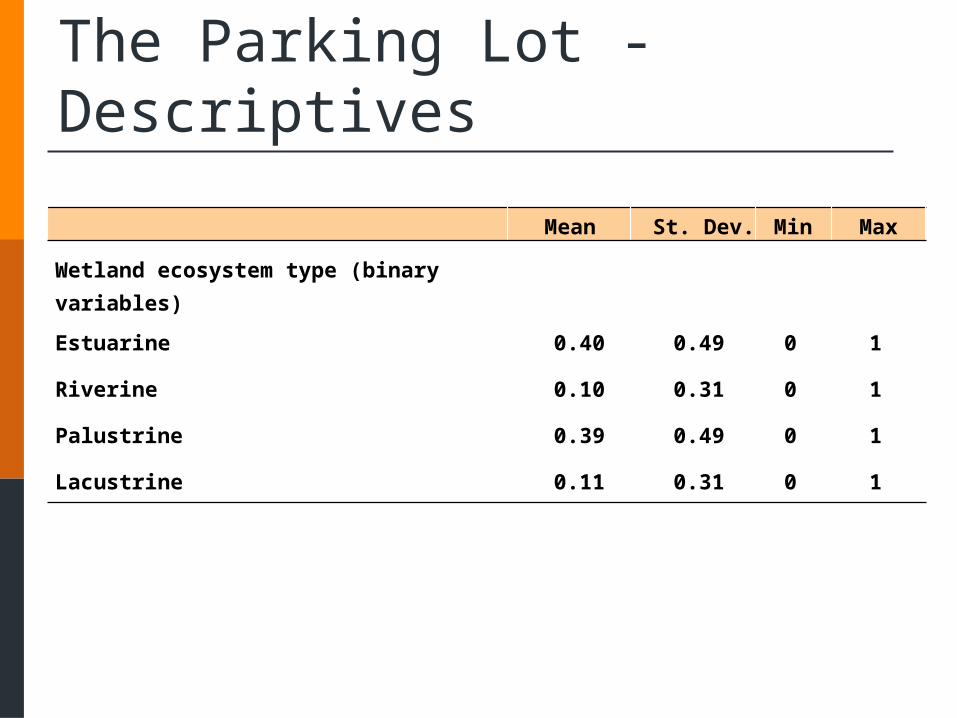
Mean St. Dev. Min Max Wetland ecosystem type (binary variables)
Estuarine 0.40 0.49 0 1
Riverine 0.10 0.31 0 1
Palustrine 0.39 0.49 0 1
Lacustrine 0.11 0.31 0 1
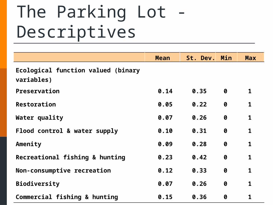
The Parking Lot - Descriptives Mean St. Dev. Min Max Ecological function valued (binary variables)
Preservation 0.14 0.35 0 1
Restoration 0.05 0.22 0 1
Water quality 0.07 0.26 0 1
Flood control & water supply 0.10 0.31 0 1
Amenity 0.09 0.28 0 1
Recreational fishing & hunting 0.23 0.42 0 1
Non-consumptive recreation 0.12 0.33 0 1
Biodiversity 0.07 0.26 0 1
Commercial fishing & hunting 0.15 0.36 0 1

The Parking Lot - Descriptives
Mean St. Dev. Min Max Geographic and socio-economic characteristics
Ramsar Site dummy 0.29 0.46 0 1
Wetland area in 50km radius (ha) 236832 244033 85 783930Population in 50km radius 616957 970885 5661 3700000
Education (county level) 23.66 9.26 11 45.4
Distance to city (km) 14.80 56.02 0 496
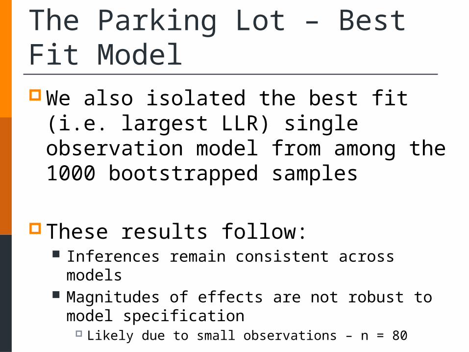
The Parking Lot – Best Fit Model We also isolated the best fit (i.e. largest LLR)
single observation model from among the 1000 bootstrapped samples
These results follow: Inferences remain consistent across models Magnitudes of effects are not robust to model specification
Likely due to small observations – n = 80
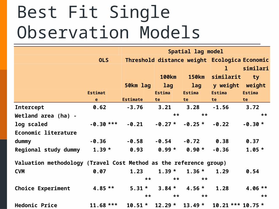
Best Fit Single Observation Models Spatial lag model
OLS Threshold distance weight Ecological similarity
weight
Economic similarity
weight50km lag 100km lag 150km lag
Estimate Estimate Estimate Estimate Estimate Estimate
Intercept 0.62 -3.76 3.21 3.28 -1.56 3.72
Wetland area (ha) - log scaled -0.30 *** -0.21 -0.27 *** -0.25 *** -0.22 -0.30 ***
Economic literature dummy -0.36 -0.58 -0.54 -0.72 0.38 0.37Regional study dummy 1.39 * 0.93 0.99 * 0.90 * -0.36 1.05 *
Valuation methodology (Travel Cost Method as the reference group)
CVM 0.07 1.23 1.39 * 1.36 * 1.29 0.54
Choice Experiment 4.85 ** 5.31 *** 3.84 *** 4.56 *** 1.28 4.06 **
Hedonic Price 11.68 *** 10.51 *** 12.29 *** 13.49 *** 10.21 *** 10.75 ***
Market Price -0.01 1.89 * 2.65 ** 3.17 ** 1.62 2.73 **
Replacement Cost 3.80 ** 3.49 *** 2.57 ** 3.32 *** 2.41 * 3.38 **
Production Function -0.07 1.72 * 2.08 ** 2.35 ** 0.48 1.21

Best Fit Single Observation Models Spatial lag model
OLS Threshold distance weight Ecological similarity
weight
Economic similarity
weight50km lag 100km lag 150km lag
Estimate Estimate Estimate Estimate Estimate Estimate
Ecological function valued
Preservation 6.64 ** 6.74 *** 2.59 ** 2.91 ** 5.41 ** 1.67Restoration 4.03 5.41 ** 2.46 * 2.12 8.72 *** -1.34Water quality 3.86 5.61 ** 1.87 0.82 6.23 ** -0.24Flood control & water supply 4.05 4.61 ** 2.02 2.20 6.83 ** 1.83
Amenity -1.65 -1.23 -7.26 *** -7.68 *** -1.61 -7.17 ***
Recreational fishing & hunting 7.15 ** 7.38 *** 2.78 ** 3.18 ** 6.96 ** 1.70
Non-consumptive recreation 7.41 ** 7.65 *** 3.41 *** 3.76 *** 7.13 *** 2.71 **
Biodiversity 8.06 ** 9.34 *** 5.66 *** 6.27 *** 7.85 *** 4.06 ***Commercial fishing & hunting 6.06 ** 4.79 ** 0.54 0.45 6.68 ** -0.09
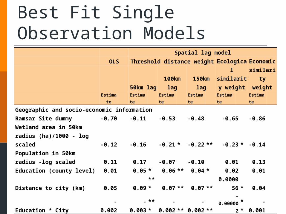
Best Fit Single Observation Models Spatial lag model
OLS Threshold distance weight Ecological similarity
weight
Economic similarity
weight50km lag 100km lag 150km lag
Estimate Estimate Estimate Estimate Estimate Estimate
Geographic and socio-economic informationRamsar Site dummy -0.70 -0.11 -0.53 -0.48 -0.65 -0.86Wetland area in 50km radius (ha)/1000 - log scaled -0.12 -0.16 -0.21 * -0.22 ** -0.23 * -0.14Population in 50km radius -log scaled 0.11 0.17 -0.07 -0.10 0.01 0.13Education (county level) 0.01 0.05 * 0.06 ** 0.04 * 0.02 0.01
Distance to city (km) 0.05 0.09 *** 0.07 ** 0.07 ** 0.000056 * 0.04
Education * City -0.002 -0.003 *** -0.002 ** -0.002 ** -0.000002 ** -0.001

Best Fit Single Observation Models Spatial lag model
OLS Threshold distance weight Ecological similarity
weight
Economic similarity
weight50km lag 100km lag 150km lag
Estimate Estimate Estimate Estimate Estimate Estimate
N 80 80 80 80 80 80
R-square 64.47%
Rho 0.22 0.27 0.29 0.23 0.16
LLR test statistic 13.82 25.83 27.80 8.16 10.39
P-value for the LLR test <0.000 *** <0.000 *** <0.000 *** <0.000**
* <0.000 ***AIC 371.33 339.09 334.81 332.84 365.16 360.82