mesoscopic physics: from brownian motion to quantum...

Mesoscopic Physics: from Brownian Motion Mesoscopic Physics: from Brownian Motion to Quantum Devices to Quantum Devices

Boris AltshulerBoris AltshulerColumbia University & Columbia University &

NEC Laboratories AmericaNEC Laboratories America

Introduction:Introduction:

History

Robert Brown (1773-1858)

The instrument with which Robert Brown studied Brownian Motion and which he used in his work on identifying the nucleus of the living cell. This instrument is preserved at the Linnean Society in London.

Brownian Motion - history

Action of water molecules pushing against the suspended object ?

Giovanni Cantoni (Pavia). N.Cimento, 27,156(1867).

Brownian Motion -history

Robert Brown, Phil.Mag. 4,161(1828); 6,161(1829)

Random motion of particles suspended in water (“dust or soot deposited on all bodies in such quantities, especially in London”)

Six papers:1. The light-quantum and the photoelectric effect.

Completed March 17.

2. A new determination of molecular dimensions. Completed April 30. Published in1906Ph.D. thesis.

3. Brownian Motion.Received by Annalen der Physik May 11.

4,5.The two papers on special relativity. Received June 30 and September 27

6. Second paper on Brownian motion.Received December 19.

Einstein’s Miraculous Year - 1905

Einstein’s Miraculous Year - 1905Six papers:1. The light-quantum and the photoelectric effect.

Completed March 17.





Einstein’s Miraculous Year - 1905Diffusion and Brownian Motion:2. A new determination of molecular dimensions.

Completed April 30. Published in1906Ph.D. thesis.



Are these papers indeed important enough to stay in the same line with the relativity and photons.Why

Q: ?

Einstein’s Miraculous Year - 1905Six papers:1. The light-quantum and the photoelectric effect.

Completed March 17.





Nobel Prize

By far the largest number of citations

The Nobel Prize in Physics 1926

"for his work on the discontinuous structure of matter, and especially for his discovery of sedimentation equilibrium"

Jean Baptiste PerrinFrance

b. 1870d. 1942

… measurements on the Brownian movement showed that Einstein's theory was in perfect agreement with reality. Through these measurements a new determination of Avogadro's number was obtained.

The Nobel Prize in Physics 1926From the Presentation Speech by Professor C.W. Oseen, member of the Nobel Committee for Physics of The Royal Swedish Academy of Sciences on December 10, 1926

1. Each molecule is too light to change the momentum of the suspended particle.

2. Does Brownian motion violate the second law of thermodynamics ?

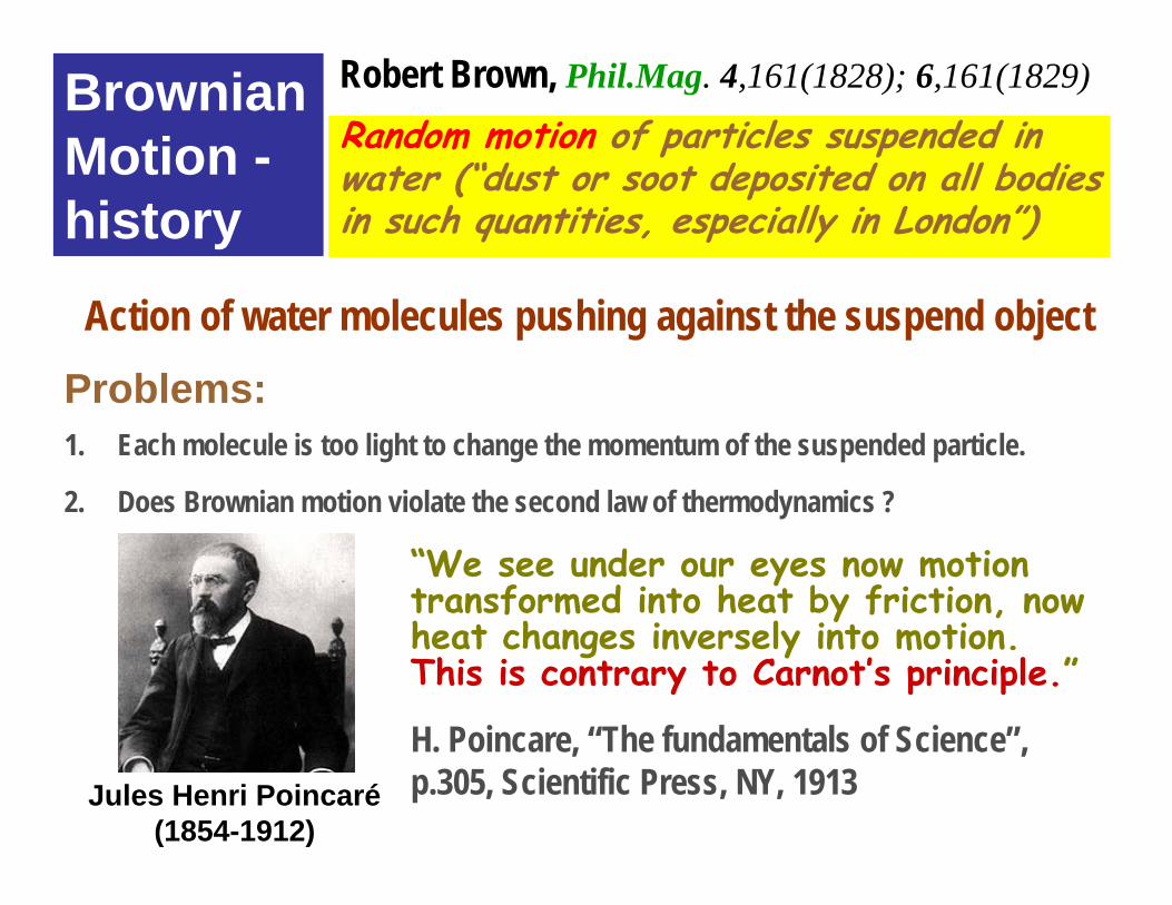
Brownian Motion -history

Robert Brown, Phil.Mag. 4,161(1828); 6,161(1829)

Random motion of particles suspended in water (“dust or soot deposited on all bodies in such quantities, especially in London”)

Action of water molecules pushing against the suspend object

Jules Henri Poincaré(1854-1912)

“We see under our eyes now motion transformed into heat by friction, now heat changes inversely into motion.This is contrary to Carnot’s principle.”

H. Poincare, “The fundamentals of Science”, p.305, Scientific Press, NY, 1913

Problems:

Problems:1. Each molecules is too light to change the momentum of the suspended particle.


3. Do molecules exist as real objects and are the laws of mechanics applicable to them?

Problems:1. Each molecules is too light to change the momentum of the suspended particle.


3. Do molecules exist as real objects and are the laws of mechanics applicable to them?

The Nobel Prize in Chemistry 1909

Wilhelm Ostwald

"in recognition of his work on catalysis and for his investigations into the fundamental principles governing chemical equilibria and rates of reaction"

“… in a purely mechanical world there could not be a before and an after as we have in our world: the tree could become a shoot and a seed again, the butterfly turn back into a caterpillar, and the old man into a child. No explanation is given by a mechanistic doctrine for the fact that this does not happen, nor can it be given because of the fundamental property of the mechanical equation. The actual irreversibility of natural phenomena thus proves the existence of processes that can not be described by mechanical equations; and with this the verdict of scientific materialism is settled.”W. OstwaldVrh. Ges. Deutsch. Naturf Arzte, 1, 155 (1895)Deutsche Gesellschaft fur Naturforscher und Arzte

Kinetic theorylogS Wk const= +

probabilityentropy

Ludwig Boltzmann1844 - 1906

logS Wk const= +

probabilityentropy

k is Boltzmann constant

( )3

3

8,exp 1

Tc

Tk

hh

π νρ νν

=⎡ ⎤⎛ ⎞ −⎜ ⎟⎢ ⎥⎝ ⎠⎣ ⎦

Kinetic theory

Ludwig Boltzmann1844 - 1906

Max Planck1858 - 1947

logS Wk const= +

From Macro to Micro

From Micro to Macro

“It is of great importance since it permits exact computation of Avogadro number … . The great significance as a matter of principle is, however … that one sees directly under the microscope part of the heat energy in the form of mechanical energy.”

Einstein, 1915

“…time reversal invariance is broken for an electron interacting with the bath produced by all other electrons.”

Dmitri S. Golubev, Andrei D. Zaikin and Gerd SchonCond-mat/0111527 v2

Brownian Motion - historyEinstein was not the first to:1. Attribute the Brownian motion to the action of water molecules pushing

against the suspended object2. Write down the diffusion equation3. Saved Second law of Thermodynamics L. Szilard, Z. Phys, 53, 840(1929)

Brownian Motion - historyEinstein was not the first to:1. Attribute the Brownian motion to the action of water molecules

pushing against the suspended object2. Write down the diffusion equation3. Saved Carnot’s principle [L. Szilard, Z. Phys, 53, 840(1929)]

By studying large molecules in solutions sugar in water or suspended particles Einstein made molecules visible

1. Apply the diffusion equation to the probability2. Derive the diffusion equation from the assumption that the process is

markovian (before Markov) and take into account nonmarkovian effects3. Derived the relation between diffusion const and viscosity

(conductivity), i.e., connected fluctuations with dissipation

Einstein was the first to:

Diffusion Equation

2 0Dtρ ρ∂

− ∇ =∂ Diffusion

constant

Einstein-Sutherland Relation

William Sutherland(1859-1911)

2 dne Dd

σ ν νμ

= ≡

If electrons would be degenerate and form a classical ideal gas

1

totTnν =

for electric conductivity σ

Einstein-Sutherland Relation for electric conductivity σ

2 dne Dd

σ ν νμ

= ≡

If electrons would be degenerate and form a classical ideal gas

1

totTnν =William Sutherland

(1859-1911)

metal( ), dn dn d dnn n eE

dx d dx dμμ

μ μ= = =

Electric field

Density of electrons

Chemical potential


dneD Edx

σ=

No current

2 dne Dd

σ ν νμ

= ≡

metal( ), dn dn d dnn n eE

dx d dx dμμ

μ μ= = =

Electric field

Density of electrons

Chemical potential

dneD Edx

σ=

Conductivity Density of states


No current

Diffusion Equation

2 0Dtρ ρ∂

− ∇ =∂

Lessons from the Einstein’s work:Universality: the equation is valid as long as the

process is marcovianCan be applied to the probability and thus

describes both fluctuations and dissipation There is a universal relation between the diffusion

constant and the viscosityStudies of the diffusion processes brings

information about micro scales.

Lesson 1:Lesson 1:

Beyond Markov chains:

Magnetoresistance and

Anderson Localization

Andrei Markov 1856-1922

•A. A. Markov. « Rasprostranenie zakona bol'shih chisel na velichiny, zavisyaschie drug ot druga ». Izvestiya Fiziko-matematicheskogo obschestva pri Kazanskom universitete, 2-ya seriya, tom 15, pp 135-156, 1906. •A. A. Markov. « Extension of the limit theorems of probability theory to a sum of variables connected in a chain ». reprinted in Appendix B of: R. Howard. Dynamic Probabilistic Systems, volume 1: Markov Chains. John Wiley and Sons, 1971.

R.A. Chentsov “On the dependence of electrical conductivity of tellurium on magnetic field at low temperatures”, Zh. Exp. Theor. Fiz. v.18, 375-385, (1948).

Quantum particle in random quenched potential

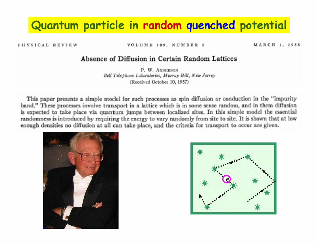
Quantum particle in random quenched potential

e

Anderson Model

• Lattice - tight binding model

• Onsite energies εi - random

• Hopping matrix elements Iijj iIij

Iij =-W < εi <Wuniformly distributed

I < Ic I > IcInsulator

All eigenstates are localizedLocalization length ξ

MetalThere appear states extended

all over the whole system

Anderson TransitionAnderson Transition

I i and j are nearest neighbors

0 otherwise

Anderson Insulator Anderson Metal

f = 3.04 GHz f = 7.33 GHz

Diffusion description fails at large scalesWhy?

Einstein: there is no diffusion at too shortscales – there is memory, i.e., the process is not marcovian.

Why there is memory at large distances in quantum case ?

ϕ1 = ϕ2


O

Constructive interference probability to return to the origin gets enhanced diffusion constant gets reduced. Tendency towards localization

pdrϕ = ∫r r

Phase accumulated when traveling along the loop

The particle can go around the loop in two directions

Φ

Magnetoresistance

No magnetic field ϕ1 = ϕ2

With magnetic field H ϕ1− ϕ2= 2∗2π Φ/Φ0

O O

Conductance2dG Lσ −=

for a cubic sample of the size L

( )( )

2

2d

g L

e DhG Lh L

ν14243

=

Einstein - Sutherland Relation for electric conductivity σ

2 dne Dd

σ ν νμ

= ≡

( )2

1 d

hD Lg LLν

=Thouless energy

mean level spacing=

dimensionlessThouless conductance

( )2

1 d

hD Lg LLν

=Thouless energy

mean level spacing=

Thouless conductance is Dimensionless

Corrections to the diffusion come from the large distances (infrared corrections)

Scaling theory of Localization(Abrahams, Anderson, Licciardello and

Ramakrishnan, 1979)

d log g( )d log L( )=β g( )

( )2

1 d

hD Lg LLν

=Thouless energy

mean level spacing=

Thouless conductance is Dimensionless

Corrections to the diffusion come from the large distances (infrared corrections)

.... Universal description!

Lesson 2:Lesson 2:

Brownian Particle as a mesoscopic system

Mesoscopic fluctuations

Mesoscopic Fluctuations.Mesoscopic Fluctuations.

×

××

××

×

××

××

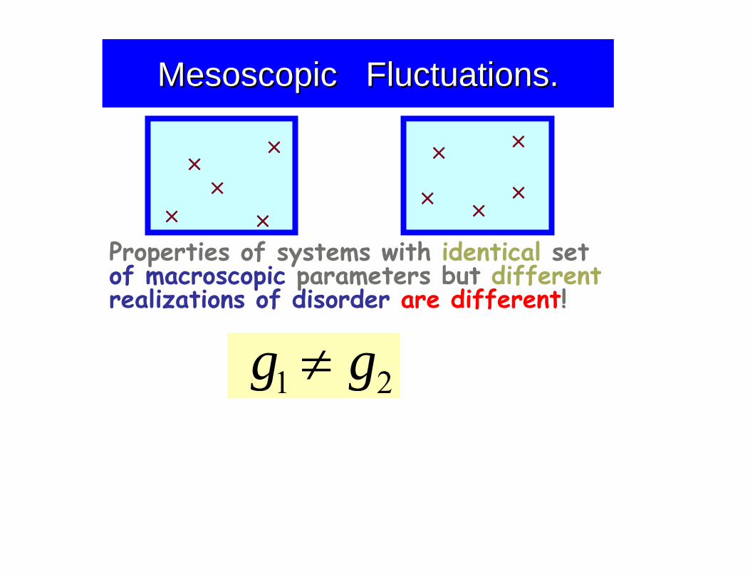
Properties of systems with identical set of macroscopic parameters but differentrealizations of disorder are different!

g1 ≠ g2

Mesoscopic Fluctuations.Mesoscopic Fluctuations.

×

××

××

×

××

××

Properties of systems with identical set of macroscopic parameters but differentrealizations of disorder are different!

g1 ≠ g2

Magnetoresistanceg H( )

H

g

... g >>1- ensemble averaging

g H( )is sample-dependent

Before Einstein:Correct question would be: describe ( )r tr

OK, maybe you can restrict yourself by ( )r tr

What is ?



Einstein: ( ) ( ) 20r r t⎡ ⎤−⎣ ⎦

r r

( ) ( )0 ?n

r r t⎡ ⎤− =⎣ ⎦r r

What is ?



Einstein: ( ) ( ) 20r r t⎡ ⎤−⎣ ⎦

r r

( ) ( )0 ?n

r r t⎡ ⎤− =⎣ ⎦r r

Mesoscopic physics: Not only

But also

( )g H

( ) ( ) 2g H g H h⎡ ⎤− +⎣ ⎦

Example

Statistics ofStatistics ofInterested in

Magnetic field or any other external tunable parameter

Time…..evolves as function of

Conductance of each sample…..

Position of each particle……

observables

Set of small conductors

Set of brownianparticles

ensemble

rr gHt

( )r tr ( )g H

( ) ( ) 2

1 2r t r tr r⎡ ⎤−⎣ ⎦ ( ) ( ) 2

1 2g H g H⎡ ⎤−⎣ ⎦

Brownian motion

Conductance fluctuations

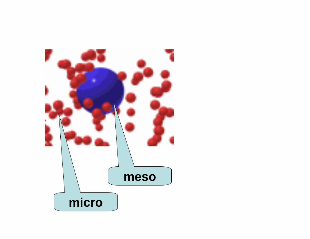
meso

micro

First paper on Quantum Theory of Solid State (Specific heat)Annalen der Physik, 22, 180, 800 (1907)

First paper on Mesoscopic PhysicsAnnalen der Physik, 17, 549 (1905)

Brownian particle was the first mesoscopic device in use

g1 ≠ g2

g1 − g2 ≅1 G1 −G2 ≅ e2 h

×

××

××

×

××

××

Magnetoresistanceg H( )

H

g

≈1 Statistics of the functions of g(H) are universal

B.A.(1985); Lee & Stone (1985)

Huibers, et al. PRL, 81 1917(1998).Huibers, et al. PRL, 81 1917(1998).

Marcus et. al, 1998

What is a Mesoscopic System?Statistical descriptionCan be effected by a microscopic system and the effect can be macroscopically detected

Meso can serve as a microscope to study micro

Magnetic impuritiesFreezing in magnetic field

F.Pierre & Norman Birge, 2002

Lesson 3:Lesson 3:

Looking for magnetic impurities in disordered

conductors

-0 .0 4 -0 .0 2 0 .0 0 0 .0 2 0 .0 4

3 .1 K

1 .1 7 K

2 1 0 m K

4 5 m K

1 0 -3

ΔR/R

B (T )

Weak Localization and dephasing rateI

V

B

L ~ 0.25 mm

ΦMagnetoresistance

No magnetic field ϕ1 = ϕ2

With magnetic field H ϕ1− ϕ2= 2∗2π Φ/Φ0

O O

I

V

BL ~ 0.25 mm

-0 .0 4 -0 .0 2 0 .0 0 0 .0 2 0 .0 4

3 .1 K

1 .1 7 K

2 1 0 m K

4 5 m K

1 0 -3

ΔR/R

B (T )

-0 .0 4 -0 .0 2 0 .0 0 0 .0 2 0 .0 4

3 .1 K

1 .1 7 K

2 1 0 m K

4 5 m K

1 0 -3

ΔR/R

B (T )

22

2H

H

R h AR LR e L L

hL D LeH

φ

φ φτ

⎛ ⎞Δ= − + ⎜ ⎟

⎝ ⎠

≡ =

L is the length of the wire

A is the wire cross-section

Dephasing rate can be measured. Can it be calculated?

hω

hω

• other electrons• phonons• magnons• two level systems••

Inelastic dephasing rate 1/τϕ

O

( )( )

tt

tδϕδ

δδ

ωδϕ⎛ ⎞ ⎛ ⎞

=⎜ ⎟ ⎜ ⎟+⎝ ⎠⎝

−

⎠h

( ) ( ) ( )2 22ϕ ϕδϕτ τδ πϕ⎡ ⎤− ≈⎣ ⎦

e-e interaction – Electric noise Fluctuation- dissipation theorem:

( ) ( )kT

kkk

TkEE

krrr

,2coth

, 2, ωσω

ωσω

αβ

βα

αβω

βα ∝⎟⎠⎞

⎜⎝⎛=

Electric noise - randomly time and space -dependent electric field . Correlation function of this field is completely determined by the conductivity :

( ) ( ), ,E r t E kα α ω⇔rr

( )ωσ ,kr

Noise intensity increases with the temperature, T, and with resistance

( )LRehLg 2)( ≡ -Thouless

conductance- resistance of the sample with size( )LR L

L Dϕ ϕτ≡ - dephasing length

- diffusion constant of the electrons

( ), ,k

TE Ek

α β

ωαβσ ω

∝r r

( )h T

g Lϕ ϕτ∝

D

( )LRehLg 2)( ≡ -Thouless

conductance- resistance of the sample with size( )LR L

L Dϕ ϕτ≡ - dephasing length

- diffusion constant of the electrons

( )h T

g Lϕ ϕτ∝

For a wire 23

1 Tϕτ

∝

D

B.A, Aronov, and Khmelnitsky, J. Phys. C (1982).

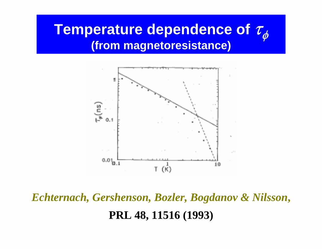
Temperature dependence of τφ(from magnetoresistance)

Echternach, Gershenson, Bozler, Bogdanov & Nilsson,PRL 48, 11516 (1993)

0.1 1

0.01

0.1

1

10 Ag 6N Au 6N

Ag 5N Cu 6N Au 4N

τ φ (ns

)

T (K)

τφ(T) in Au wires

0.1 1

0.01

0.1

1

10 Ag 6N Au 6N

Ag 5N Cu 6N Au 4N

τ φ (ns

)

T (K)

τφ(T) in Ag, Au & Cu wires

T-2/3

Saturation is sample dependent

• Ag 6N, Au 6N→ agreement with AAK theory

• Ag 5N, Cu 6N→ saturation of τφ(T)

• Au 4N→ contains ~ 30 ppm of Fe

0.1 1

0.01

0.1

1

10 Ag 6N Au 6N

Ag 5N Cu 6N Au 4N

τ φ (ns

)

T (K)



Low T behavior vs. Purity:

T-2/3

x

xN = 99.9…9 % source material purity

• Ag 6N, Au 6N→ agreement with AAK theory

• Ag 5N, Cu 6N→ saturation of τφ(T)

• Au 4N→ contains ~ 30 ppm of Fe

0.1 1

0.01

0.1

1

10 Ag 6N Au 6N

Ag 5N Cu 6N Au 4N

τ φ (ns

)

T (K)



Low T behavior vs. Purity:

T-2/3 xN = 99.9…9 % source material purity

x

Magnetic Impurities: the Kondo Effect

e

e

J .Sσur ur

Spin-flip scattering

increased resistivity reduction of τφ

Collective effect:Formation of a

singlet spin state

T

R

KT

Log(T)−β

sfγ

T

spin-flip

(total scattering rate)

phononsKondo

J1/νFKB eETk −≈

Au with and without Feimpurities

0.0 0.1 0.2 0.3 0.4 0.5 0.6 0.70.0 0.1 0.2 0.3 0.4 0.5 0.6 0.70.0

0.5

1.0

1.5

2.0

2.5

3.0

3.5

4.0

exp. α/T1/2 - β Ln(T) α/T1/2

α=1.65 10-4 K-1/2

β=1.23 10-3

T (K)

Au2

δR/R

(0 / 00)

exp. α/T1/2

α=2.7 10-4 K-1/2

AuMSU

T (K)

Kondo effect: R(T) = A - B log(T)

T-invariance is clearly violated, therefore we have dephasing

Magnetic Impurities- before - after

0.1 1

0.1

1

10

TK

6N silver:5N silver:

e--e- & e--ph

τ φ (ns

)

T (K)

bare 0.3 ppm Mn implanted 1 ppm Mn implanted

Dephasing and temperature dependence of the resistivity.

1 ppm of Mn is invisible in R(T)

1 2 3 4

0.2

0.4

0.6

0.8

1.0

1.2

δR/R

(‰)

T-1/2 (K-1/2)

Ag with 1 ppm Mn at B=30mT Fit: 2.4E-4T-1/2

TKondo

Can magnetic impurities cause an apparent saturation of τφ ?

YES! But only if T ≈ TKondo

0.1 1

1

10 Ag (6N)

Ag (5N) bare

1.0ppm Mn

0.3ppm Mn

e-e & e-ph scattering

spin-flipscattering

TKondo

τ φ (ns

)

T (K)

τφ(TK) =h νF

4 nimp

0.6 nscimp (ppm)≈

Spin-flip rate peaks at TK:

Is it a proof of the magnetic impurities domination in the decoherence ? Not yet

-0 .0 4 -0 .0 2 0 .0 0 0 .0 2 0 .0 4

3 .1 K

1 .1 7 K

2 1 0 m K

4 5 m K

1 0 -3

ΔR/R

B (T )

Phase relaxation

rate

I

V

BL ~ 0.25 mm

Energy relaxation?

-0 .0 4 -0 .0 2 0 .0 0 0 .0 2 0 .0 4

3 .1 K

1 .1 7 K

2 1 0 m K

4 5 m K

1 0 -3

ΔR/R

B (T ) -0.6 -0.4 -0.2 0.0 0.2 0.4 0.610

20

V (mV)

dI/d

V (µ

S)

-0.6 -0.4 -0.2 0.0 0.2 0.4 0.60

20

40

60

80

100

V (mV)

dI/d

V (µ

S)

-0.6 -0.4 -0.2 0.0 0.2 0.4 0.60

20

40

60

80

100

V (mV)

dI/d

V (µ

S)

-0.6 -0.4 -0.2 0.0 0.2 0.4 0.610

20

V (mV)

dI/d

V (µ

S)

-0.2 0.00

1

E (meV)

f(E)

-0.2 0.00

1

E (meV)

f(E)

UU

VS V

U

R

U

U=0

U=0.2mV

I

V

BL ~ 0.25 mm

Phase relaxation

rateDeconvolution

Energy relaxation

Energy relaxation?

-0 .0 4 -0 .0 2 0 .0 0 0 .0 2 0 .0 4

3 .1 K

1 .1 7 K

2 1 0 m K

4 5 m K

1 0 -3

ΔR/R

B (T ) -0.6 -0.4 -0.2 0.0 0.2 0.4 0.610

20

V (mV)

dI/d

V (µ

S)

-0.6 -0.4 -0.2 0.0 0.2 0.4 0.60

20

40

60

80

100

V (mV)

dI/d

V (µ

S)

-0.6 -0.4 -0.2 0.0 0.2 0.4 0.60

20

40

60

80

100

V (mV)

dI/d

V (µ

S)

-0.6 -0.4 -0.2 0.0 0.2 0.4 0.610

20

V (mV)

dI/d

V (µ

S)

-0.2 0.00

1

E (meV)

f(E)

-0.2 0.00

1

E (meV)

f(E)

UU

VS V

U

R

U

U=0

U=0.2mV

I

V

BL ~ 0.25 mm

Phase relaxation

rateDeconvolution

Energy relaxation

Energy relaxation?

B=0 onlyCan be doneat nonzero B

ε ε

One electron can not change energy after scattering by a system of two degenerated states.

ε

ε1

ε−ω

ε1+ω

Two electrons can exchange energy in spite of the fact that the states of the impurity are degenerate and it can not be excited

One electron can not change energy after scattering by a system of two degenerated states.

Second order in electron –impurity exchange

Controlled experiment II: energy exchange

Ag (99.9999%)

0.7 ppm Mn2+

implantation

Comparativeexperiments

bare

implanted

Effect of 1 ppm Mn on interactions ?

Left as is

25 nm

106 Ag1Mn

Concentration of Mn impurities

Energy relaxation

Dephasing timeτφ

?Neutralization current+

Monte Carlo simulations

Implanted wirecim

“Bare” wirecb

( )0.7 0.1bc

ppm+

±

Hugues POTHIER

Norman BIRGE


Dephasing timeτφ



Implanted wirecim

“Bare” wirecb

( )0.7 0.1bc

ppm+

±

( )0.95 0.1 ppm±( )0.1 0.01 ppm±

-0.2 0.0 0.2

0.9

1.0

-0.2 0.0 0.2

0.8

0.9

V (mV)

Rtd

I/dV

Energy relaxation at weak B

U = 0.1 mVB = 0.3 T

weak interaction

strong interaction

bare

implanted

Rtd

I/dV

U

( )

-0.5 0.0 0.5

0.9

1.0

V (mV)

Rtd

I/dV

( )

-0.5 0.0 0.5

0.9

1.0

V (mV)

Rtd

I/dV

-0.2 0.0 0.2

0.9

1.0

-0.2 0.0 0.2

0.8

0.9

V (mV)U = 0.1 mVB = 0.3 TB = 2.1 T

Rtd

I/dV

Rtd

I/dV

Very weakinteraction

bare

implanted

Energy relaxation at weak and strong B

H

τε−1

g Hμ ε

First order

Second order

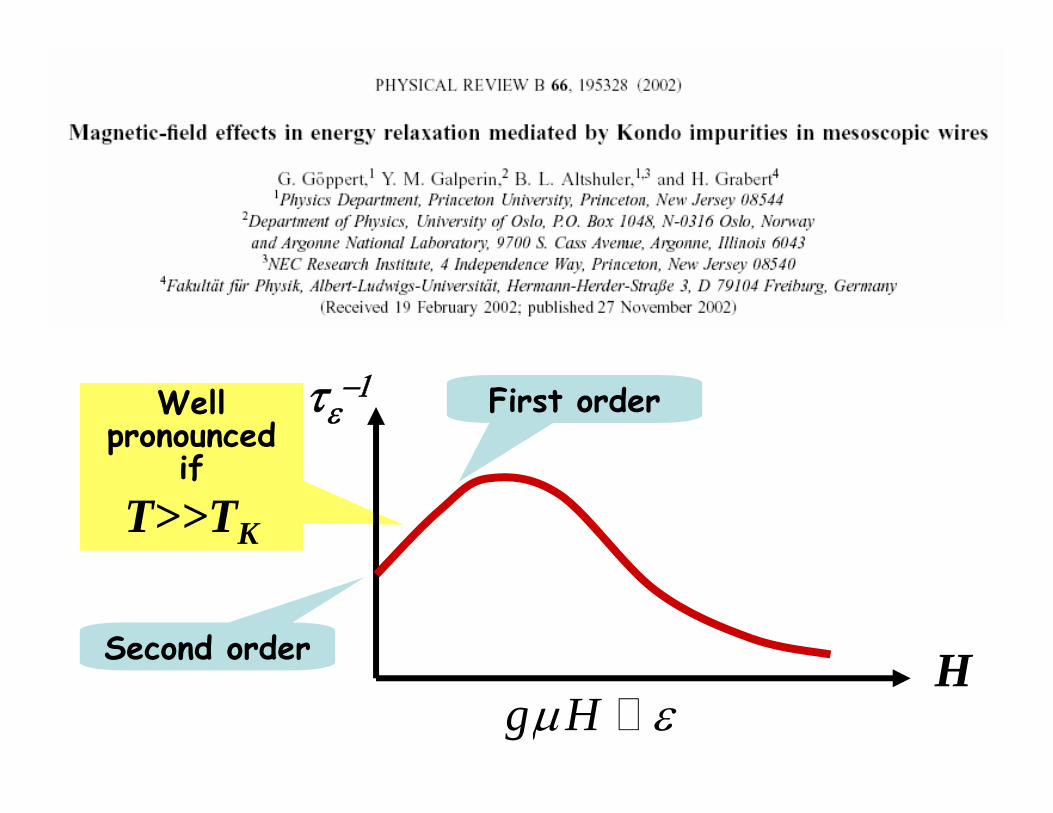
Well pronounced

ifT>>TK

H

τε−1

g Hμ εSecond order

First order


Energy relaxation

Dephasing timeτφ



Implanted wirecim

“Bare” wirecb

( )0.7 0.1bc

ppm+

±

( )0.95 0.1 ppm±

( )0.9 0.3 ppm±

( )0.1 0.01 ppm±

1 Dephasing and energy relaxation give very close concentration of the magnetic impurities

2 Energy relaxation is suppressed by the magnetic field as was predicted

Mn impurities dominate both energy and phase relaxation in this temperature interval. No room for mysteries like zero-point dephasing.

Both energy and phase relaxation times should increase dramatically when temperature is reduces further –Kondo effect

Both energy and phase relaxation times should increase dramatically when temperature is reduces further – Kondo effect

0.1 1

0.01

0.1

1

10 Ag 6N Au 6N

Ag 5N Cu 6N Au 4N

τ φ (ns

)

T (K)

FeTK=0.8K

MnTK=0.02K

Instead of Conclusions:Instead of Conclusions:

Quantum ComputerAnd

Quantum Devices

Simulations v = 10 γ0 1 20.1

1 /2 5,1000 runsv γ =

12τ

Simulations

1000 shots

12τ

/2 0.8v γ =

/2 5v γ =

Analitics

( ) 12212

21 sine t e vv

γτ γ τ− ⎛ ⎞Ψ = +⎜ ⎟⎝ ⎠

0 1 2

1

100 shots100 shots

Single fluctuator Two parameters:Switching rate γCoupling constant v

Quantum Devices are Unavoidably Mesoscopic Systems:•All measurements should be probabilistic

•They are extremely sensitive to the environment

Bad Qubit might be an excellent research device

mesoscopic physics: from brownian motion to quantum...

Documents