meso-scale finite element simulation of deformation
TRANSCRIPT

MESO-SCALE FINITE ELEMENT SIMULATION OF DEFORMATION
BANDING IN FLUID-SATURATED SANDS
A DISSERTATION
SUBMITTED TO THE DEPARTMENT OF CIVIL AND ENVIRONMENTAL
ENGINEERING
AND THE COMMITTEE ON GRADUATE STUDIES
OF STANFORD UNIVERSITY
IN PARTIAL FULFILLMENT OF THE REQUIREMENTS
FOR THE DEGREE OF
DOCTOR OF PHILOSOPHY
Jose E. Andrade
June 2006

c© Copyright by Jose E. Andrade 2006
All Rights Reserved
ii

I certify that I have read this dissertation and that, in my opinion, it is fully
adequate in scope and quality as a dissertation for the degree of Doctor of
Philosophy.
Ronaldo I. Borja Principal Adviser
I certify that I have read this dissertation and that, in my opinion, it is fully
adequate in scope and quality as a dissertation for the degree of Doctor of
Philosophy.
Peter M. Pinsky
I certify that I have read this dissertation and that, in my opinion, it is fully
adequate in scope and quality as a dissertation for the degree of Doctor of
Philosophy.
Ruben Juanes
Approved for the University Committee on Graduate Studies.
iii

iv

Abstract
Deformation banding is a ubiquitous failure mode in geomaterials such as rocks, concrete,
and soils. It is well known that these bands of intense localized deformation can signif-
icantly reduce the load-carrying capacity of structures. Furthermore, when dealing with
fluids-saturated geomaterials, the interplay between the compaction/dilation of pores and
development of pore fluid pressures is expected to control not only the strength of the solid
matrix but also its ability to block or transport such fluids. Accurate and thorough sim-
ulation of these phenomena (i.e. deformation banding and fluid flow) is challenging, as it
requires numerical models capable of capturing micro-mechanical processes such as mineral
particle rolling and sliding in granular soils and the coupling between porosity and relative
permeability, while still maintaining a continuum mechanics framework. Until recently,
these processes could not even be observed in the laboratory. Numerical models could only
interpret material behavior as a macroscopic process and were, therefore, unable to model
the very complex behavior of saturated geomaterials accurately.
In this dissertation, we propose a numerical model capable of capturing some of the most
intricate and important features of sand behavior. Development of the model is further mo-
tivated by new advances in laboratory experimentation that allow for the observation of
key parameters associated with material strength at a scale finer than specimen scale. One
such parameter is porosity, a relative measure of the amount of voids in a soil sample. A
novel elastoplastic constitutive model based on a meso-scale description of the porosity is
proposed to simulate the behavior of the underlying sand matrix and to accurately predict
the development of deformation bands in saturated samples. ‘Meso-scale’ is defined here
as a scale smaller than specimen size but larger than particle size. The effect of meso-scale
inhomogeneities on the deformation-diffusion behavior of loose and dense sands is stud-
ied by casting the meso-scale constitutive model within a mixed nonlinear finite element
v

framework. The main findings of this work are that meso-scale imperfections (in macro-
scopically homogeneous samples) are responsible for triggering deformation bands, which
tend to strongly influence the direction and volume of fluid flow. Numerical simulations
clearly show that failure and flow modes in dense sands are sharply distinct from those in
loose sands. It is concluded that meso-scale inhomogeneities, which are inevitably present in
‘homogeneous’ samples of sand, play a crucial role in the mechanical behavior of specimens
under drained and undrained conditions at finite strains.
vi

Acknowledgments
I would like to express my sincerest gratitude to my academic advisor, Ronaldo Borja.
Ronnie has gradually guided me towards becoming a critical thinker and an independent
researcher. This dissertation is the product of his guidance and encouragement.
The dissertation committee has also played an important role in the completion of this
thesis. Peter Pinsky has been a member of the reading committee but also a great teacher
and advisor. I am grateful to Ruben Juanes for his constructive criticism of this work and
for his advice on academic matters. Adrian Lew has not only been part of the dissertation
committee but has also been a friend who has always stimulated me intellectually with his
insatiable inquisitive style. Finally, I am grateful to Keith Loague for serving as chair of
the dissertation committee.
The Blume and Shah families provided for three academic years of financial support in
the form of fellowships and made possible my post-graduate studies at Stanford. Without
their financial support, I would not have been able to come to Stanford and this dissertation
would not have been possible. Once again, I would like to express my deepest gratitude to
these two families who have made it possible for many graduate students to achieve their
dreams. The remainder of my post-graduate study was funded by research assistantships
through grant numbers CMS-0201317 and CMS-0324674 from the National Science Foun-
dation. This support is gratefully acknowledged.
At Stanford, I have been blessed with wonderful friends. The five years I spent here
with my family have been the most wonderful years of my life. My co-workers and friends
at the John A. Blume Earthquake Engineering Center, have been people who have not only
inspired me intellectually, but also have made my stay here a more pleasant one by offering
me their friendship.
Finally, I want to thank the most important people in my life: my family. My parents
have been a constant source of encouragement ever since I was a child. My parents were
vii

my first teachers; they taught me the most important things in life and it is to them that I
owe who I am as a person (though the negative parts of my character are my own device).
My wife Claudia has been my ideal companion for eight years. She is my dearest friend,
confidant, partner and advisor. She believed in me even when I did not. Now as parents,
we share the blessing of having a wonderful daughter. Milena was born two years ago and
ever since she arrived she became the center of my universe. It is to Milena that I dedicate
this dissertation.
viii

To Milena
ix

x

Contents
Abstract v
Acknowledgments vii
1 Introduction 1
1.1 Objectives and statement of the problem . . . . . . . . . . . . . . . . . . . . 1
1.2 Motivation . . . . . . . . . . . . . . . . . . . . . . . . . . . . . . . . . . . . 2
1.3 Methodology . . . . . . . . . . . . . . . . . . . . . . . . . . . . . . . . . . . 3
1.4 Structure of presentation . . . . . . . . . . . . . . . . . . . . . . . . . . . . . 4
2 Background Literature 7
2.1 Strain localization in the lab and in the field . . . . . . . . . . . . . . . . . . 7
2.2 Strain localization analysis and simulation . . . . . . . . . . . . . . . . . . . 9
2.3 Mechanical behavior and constitutive models for sands . . . . . . . . . . . . 11
3 Meso-scale simulation of granular media 19
3.1 Introduction . . . . . . . . . . . . . . . . . . . . . . . . . . . . . . . . . . . . 20
3.2 Formulation of the infinitesimal model . . . . . . . . . . . . . . . . . . . . . 23
3.2.1 Hyperelastic response . . . . . . . . . . . . . . . . . . . . . . . . . . 23
3.2.2 Yield surface, plastic potential function, and flow rule . . . . . . . . 24
3.2.3 State parameter and plastic dilatancy . . . . . . . . . . . . . . . . . 27
3.2.4 Consistency condition and hardening law . . . . . . . . . . . . . . . 30
3.2.5 Implications to entropy production . . . . . . . . . . . . . . . . . . . 31
3.2.6 Numerical implementation . . . . . . . . . . . . . . . . . . . . . . . . 33
3.2.7 Algorithmic tangent operator . . . . . . . . . . . . . . . . . . . . . . 38
3.3 Finite deformation plasticity . . . . . . . . . . . . . . . . . . . . . . . . . . . 41
xi

3.3.1 Entropy inequality . . . . . . . . . . . . . . . . . . . . . . . . . . . . 41
3.3.2 Finite deformation plasticity model . . . . . . . . . . . . . . . . . . . 43
3.3.3 Numerical implementation . . . . . . . . . . . . . . . . . . . . . . . . 45
3.3.4 Algorithmic tangent operator . . . . . . . . . . . . . . . . . . . . . . 48
3.3.5 Localization condition . . . . . . . . . . . . . . . . . . . . . . . . . . 51
3.4 Numerical simulations . . . . . . . . . . . . . . . . . . . . . . . . . . . . . . 52
3.4.1 Plane strain simulation . . . . . . . . . . . . . . . . . . . . . . . . . 53
3.4.2 Three-dimensional simulation . . . . . . . . . . . . . . . . . . . . . . 57
3.5 Closure . . . . . . . . . . . . . . . . . . . . . . . . . . . . . . . . . . . . . . 61
4 Strain localization in dense sands 65
4.1 Introduction . . . . . . . . . . . . . . . . . . . . . . . . . . . . . . . . . . . . 66
4.2 Constitutive assumptions . . . . . . . . . . . . . . . . . . . . . . . . . . . . 69
4.2.1 The hyperelastic model . . . . . . . . . . . . . . . . . . . . . . . . . 69
4.2.2 Yield surface, plastic potential, their derivatives and the flow rule . . 71
4.2.3 Maximum plastic dilatancy, hardening law and the consistency con-
dition . . . . . . . . . . . . . . . . . . . . . . . . . . . . . . . . . . . 76
4.3 Numerical implementation . . . . . . . . . . . . . . . . . . . . . . . . . . . . 78
4.3.1 Local return mapping algorithm . . . . . . . . . . . . . . . . . . . . 78
4.3.2 Consistent tangent in principal directions . . . . . . . . . . . . . . . 83
4.4 Consistent tangent operators . . . . . . . . . . . . . . . . . . . . . . . . . . 84
4.5 Search algorithm in principal stress space . . . . . . . . . . . . . . . . . . . 86
4.6 Numerical examples . . . . . . . . . . . . . . . . . . . . . . . . . . . . . . . 90
4.6.1 Stress-point simulations . . . . . . . . . . . . . . . . . . . . . . . . . 91
4.6.2 Simulations with cubical specimens . . . . . . . . . . . . . . . . . . . 93
4.6.3 Simulations with cylindrical specimens . . . . . . . . . . . . . . . . . 100
4.7 Closure . . . . . . . . . . . . . . . . . . . . . . . . . . . . . . . . . . . . . . 103
5 Modeling deformation banding in saturated sands 107
5.1 Introduction . . . . . . . . . . . . . . . . . . . . . . . . . . . . . . . . . . . . 108
5.2 Balance laws: conservation of mass and linear momentum . . . . . . . . . . 111
5.2.1 Balance of mass . . . . . . . . . . . . . . . . . . . . . . . . . . . . . 112
5.2.2 Balance of linear momentum . . . . . . . . . . . . . . . . . . . . . . 115
5.3 Constitutive framework . . . . . . . . . . . . . . . . . . . . . . . . . . . . . 117
xii

5.3.1 The elastoplastic model for granular media . . . . . . . . . . . . . . 117
5.3.2 Darcy’s law . . . . . . . . . . . . . . . . . . . . . . . . . . . . . . . . 122
5.4 Finite element implementation . . . . . . . . . . . . . . . . . . . . . . . . . 123
5.4.1 The strong form . . . . . . . . . . . . . . . . . . . . . . . . . . . . . 124
5.4.2 The variational form . . . . . . . . . . . . . . . . . . . . . . . . . . . 125
5.4.3 The matrix form . . . . . . . . . . . . . . . . . . . . . . . . . . . . . 131
5.5 Localization of saturated granular media . . . . . . . . . . . . . . . . . . . . 133
5.6 Numerical simulations . . . . . . . . . . . . . . . . . . . . . . . . . . . . . . 135
5.6.1 Plane strain compression in globally undrained dense sands . . . . . 136
5.6.2 Plane strain compression in globally undrained loose sands . . . . . 143
5.7 Conclusion . . . . . . . . . . . . . . . . . . . . . . . . . . . . . . . . . . . . 154
6 Conclusion and future work 155
A Mixed formulation 159
xiii

xiv

List of Tables
3.1 Summary of rate equations for plasticity model for sands, infinitesimal de-
formation version. . . . . . . . . . . . . . . . . . . . . . . . . . . . . . . . . 34
3.2 Return mapping algorithm for plasticity model for sands, infinitesimal defor-
mation version. . . . . . . . . . . . . . . . . . . . . . . . . . . . . . . . . . . 35
3.3 Summary of rate equations for plasticity model for sands, finite deformation
version. . . . . . . . . . . . . . . . . . . . . . . . . . . . . . . . . . . . . . . 44
3.4 Return mapping algorithm for plasticity model for sands, finite deformation
version. . . . . . . . . . . . . . . . . . . . . . . . . . . . . . . . . . . . . . . 46
3.5 Summary of hyperelastic material parameters (see [1] for laboratory testing
procedure). . . . . . . . . . . . . . . . . . . . . . . . . . . . . . . . . . . . . 55
3.6 Summary of plastic material parameters (see [2] for laboratory testing pro-
cedure). . . . . . . . . . . . . . . . . . . . . . . . . . . . . . . . . . . . . . . 55
4.1 Summary of rate equations in three-invariant elastoplastic model for sands. 79
4.2 Return mapping algorithm for three-invariant elastoplastic model for sands. 80
5.1 Summary of hyperelastic material parameters for plane strain compression
problems. . . . . . . . . . . . . . . . . . . . . . . . . . . . . . . . . . . . . . 136
5.2 Summary of plastic material parameters for plane strain compression problems.136
xv

xvi

List of Figures
1.1 Group of apartment buildings in Niigata, Japan after a magnitude 6.5 earth-
quake rocked the town in 1964. The buildings failed due to loss of bearing
capacity when the soil beneath liquefied (after Kramer [3]). . . . . . . . . . 3
2.1 Typical failure mode for plane strain specimen (after Alshibli et al. [4]). . . 8
2.2 Extensive landsliding in Neela Dandi Mountain, north of Muzaffarabad (after
Durrani et al. [5]). . . . . . . . . . . . . . . . . . . . . . . . . . . . . . . . . 9
2.3 Compression plane for typical soil sample (after Schofield and Wroth [6]). . 12
2.4 Data of yielding deduced from triaxial tests on undisturbed Winnipeg clay
in effective stress plane (after Graham et al. [7]). . . . . . . . . . . . . . . . 13
2.5 Yield surfaces and data obtained from Monterey sand in principal effective
stress space (after Lade and Duncan [8]). . . . . . . . . . . . . . . . . . . . 14
2.6 Macroscopic responses from triaxial compression in dense and loose sands.
Top: Deviartoric stress versus axial strain. Bottom: Volumetric strain versus
axial strain (after Cornforth [9]). . . . . . . . . . . . . . . . . . . . . . . . . 15
2.7 Yield loci and plastic potentials for dense Ottawa sand proposed by Poorooshasb
et al. [10, 11]. . . . . . . . . . . . . . . . . . . . . . . . . . . . . . . . . . . . 17
3.1 Cross-section through a biaxial specimen of silica sand analyzed by X-ray
computed tomography; white spot is a piece of gravel. . . . . . . . . . . . . 21
3.2 Comparison of shapes of critical state yield surfaces. . . . . . . . . . . . . . 25
3.3 Yield function and family of plastic potential surfaces. . . . . . . . . . . . . 26
3.4 Geometric representation of state parameter ψ. . . . . . . . . . . . . . . . . 29
3.5 Finite element mesh for plane strain compression problem. . . . . . . . . . . 54
3.6 Load-time functions. . . . . . . . . . . . . . . . . . . . . . . . . . . . . . . . 54
3.7 Initial specific volume for plane strain compression problem. . . . . . . . . . 56
xvii

3.8 Contours of: (a) determinant function; and (b) deviatoric invariant of loga-
rithmic stretches at onset of localization. . . . . . . . . . . . . . . . . . . . . 56
3.9 Contours of: (a) plastic hardening modulus; and (b) volumetric invariant of
logarithmic stretches at onset of strain localization. . . . . . . . . . . . . . . 57
3.10 Finite element mesh and initial specific volume for 3D compression problem. 58
3.11 Nominal axial stress-axial strain responses for 3D compression problem. . . 59
3.12 Volume change-nominal axial strain responses for 3D compression problem. 59
3.13 Stress path for homogeneous specimen simulation with finite deformation. . 60
3.14 Determinant function at onset of localization. . . . . . . . . . . . . . . . . . 61
3.15 Deviatoric invariant of logarithmic stretches at onset of strain localization. . 62
3.16 Volumetric invariant of logarithmic stretches at onset of strain localization. 62
3.17 Deformed finite element mesh at onset of localization (deformation magnified
by a factor of 3). . . . . . . . . . . . . . . . . . . . . . . . . . . . . . . . . . 63
3.18 Convergence profiles of global Newton iterations: finite deformation simula-
tion of heterogeneous specimen with B-bar. . . . . . . . . . . . . . . . . . . 63
4.1 Three-invariant yield surface in Kirchhoff stress space for ρ = 0.78. (a) Cross-
section on deviatoric plane, dashed line represents two-invariant counterpart
for comparison and (b) three-dimensinal view. . . . . . . . . . . . . . . . . . 72
4.2 Reference frame in principal directions basis. . . . . . . . . . . . . . . . . . 88
4.3 Stress paths on meridian plane. Yield surfaces expand from A to B and to
C whereas stress paths follow O–A′–B′–C ′ trajectory. . . . . . . . . . . . . 92
4.4 Stress paths on deviatoric plane. Yield surfaces expand from A to B and to
C whereas stress paths follow O–A′–B′–C ′ trajectory. . . . . . . . . . . . . 93
4.5 Minimum determinant of the acoustic tensor at various load steps. . . . . . 94
4.6 Profile of the determinant of the acoustic tensor for three-invariant model
with ρ = 0.7 at onset of localization. . . . . . . . . . . . . . . . . . . . . . . 94
4.7 Convergence profile for search algorithm at various load steps. . . . . . . . . 95
4.8 Initial specific volume field and finite element discretization for inhomoge-
neous rectangular specimens. . . . . . . . . . . . . . . . . . . . . . . . . . . 97
4.9 Contour of function F (A) at onset of localization for inhomogeneous rect-
angular specimens. . . . . . . . . . . . . . . . . . . . . . . . . . . . . . . . . 98
xviii

4.10 Deviatoric strain invariant field at onset of localization for inhomogeneous
rectangular specimens. . . . . . . . . . . . . . . . . . . . . . . . . . . . . . . 98
4.11 Nominal axial stress response for rectangular specimens. . . . . . . . . . . . 99
4.12 Volume change response for rectangular specimens. . . . . . . . . . . . . . . 100
4.13 Initial specific volume field and finite element discretization for inhomoge-
neous cylindrical specimens. . . . . . . . . . . . . . . . . . . . . . . . . . . . 101
4.14 Total deviatoric strain invariant on various cut-planes at the onset of local-
ization for sample ‘INHOMO 1.58-1.61’. . . . . . . . . . . . . . . . . . . . . 102
4.15 Determinant of acoustic tensor on various cut-planes at the onset of localiza-
tion for sample ‘INHOMO 1.58-1.61’. . . . . . . . . . . . . . . . . . . . . . . 102
4.16 Nominal axial stress response for cylindrical specimens. . . . . . . . . . . . 103
4.17 Volume change response for cylindrical specimens. . . . . . . . . . . . . . . 104
4.18 Convergence profile for finite element solution at various load steps. . . . . 104
5.1 Current configuration Ω mapped from respective solid and fluid reference
configurations. . . . . . . . . . . . . . . . . . . . . . . . . . . . . . . . . . . 113
5.2 Nondimensional values of intrinsic permeability (i.e. k/d2) as a function of
specific volume v. . . . . . . . . . . . . . . . . . . . . . . . . . . . . . . . . . 124
5.3 Reference domain Ω0 with decomposed boundary Γ0 . . . . . . . . . . . . . 125
5.4 Initial specific volume for dense sand specimen superimposed on undeformed
finite element mesh. . . . . . . . . . . . . . . . . . . . . . . . . . . . . . . . 137
5.5 (a) Contour of the determinant function for the drained acoustic tensor at a
nominal axial strain of 5% and (b) deviatoric strains in contour with super-
imposed relative flow vectors q at 5% axial strain for dense sand sample. . . 139
5.6 (a) Volumetric strain contour superimposed on deformed finite element mesh
at 5% axial strain and (b) contour of Cauchy fluid pressure p on deformed
sample at 5% axial strain (in kPa) for dense sand sample. Dotted lines
delineate undeformed configuration. . . . . . . . . . . . . . . . . . . . . . . 140
5.7 Force-displacement curve for inhomogeneous and homogeneous samples of
dense sand. . . . . . . . . . . . . . . . . . . . . . . . . . . . . . . . . . . . . 141
5.8 Normalized determinant functions at point A for dense sand sample. . . . . 141
5.9 (a) Deviatoric strain invariant at Gauss point A for sample of dense sand (b)
volumetric strain invariant at Gauss point A for sample of dense sand. . . . 142
xix
5.10 Specific volume plot as a function of effective pressure at point A for dense
sand sample . . . . . . . . . . . . . . . . . . . . . . . . . . . . . . . . . . . . 143
5.11 Initial specific volume for loose sand specimen superimposed on undeformed
finite element mesh. . . . . . . . . . . . . . . . . . . . . . . . . . . . . . . . 144
5.12 (a) Contour of the determinant function for the undrained acoustic tensor
at a nominal axial strain of 5% and (b) deviatoric strains in contour with
superimposed relative flow vectors q at 5% axial strain for loose sand sample. 145
5.13 (a) Volumetric strain contour superimposed on deformed finite element mesh
at 5% axial strain and (b) contour of Cauchy fluid pressure p on deformed
sample at 5% axial strain (in kPa) for loose sand sample. Dotted lines delin-
eate undeformed configuration. . . . . . . . . . . . . . . . . . . . . . . . . . 146
5.14 Force-displacement curve for inhomogeneous and homogeneous samples of
loose sand. . . . . . . . . . . . . . . . . . . . . . . . . . . . . . . . . . . . . 147
5.15 Normalized determinant functions at point A for loose sand sample. . . . . 148
5.16 (a) Deviatoric strain invariant at Gauss point A for sample of loose sand (b)
volumetric strain invariant at Gauss point A for sample of loose sand. . . . 149
5.17 Specific volume plot as a function of effective pressure at point A for loose
sand sample . . . . . . . . . . . . . . . . . . . . . . . . . . . . . . . . . . . . 150
5.18 Convergence profile at various values of axial strain for plane strain compres-
sion test on sample of loose sand. . . . . . . . . . . . . . . . . . . . . . . . . 151
5.19 Perturbed samples of dense sand with otherwise homogeneous specific volume
v = 1.572. (a) Mesh composed of 50 Q9P4 elements and (b) mesh composed
of 200 Q9P4. . . . . . . . . . . . . . . . . . . . . . . . . . . . . . . . . . . . 152
5.20 Force displacement curves comparing perfectly homogeneous response to that
of perturbed samples . . . . . . . . . . . . . . . . . . . . . . . . . . . . . . . 153
5.21 Deviatoric strains in contours with superimposed relative flow vectors q at
3% axial strain for (a) 50 element mesh and (b) 200 element mesh . . . . . 153
xx
Chapter 1
Introduction
1.1 Objectives and statement of the problem
The main objective of this dissertation is to develop a realistic numerical model for the
detection of deformation banding in saturated granular media. Because of the complexity
of the deformation phenomenon and its interaction with the fluid flow, it is imperative
to develop a model that realistically accounts for the effective behavior of the underlying
granular material. In particular, a constitutive model capable of including inhomogeneities
in key strength parameters at the meso-scale is needed to study the effect of such inhomo-
geneities in the stability of samples of sand. The meso-scale here refers to a scale that is
smaller than specimen size (centimeter scale), but larger than a typical grain (micrometer
scale). Thus, in a typical sample encountered in the laboratory, the meso-scale would be
the millimeter scale.
Deformation banding is a phenomenon that is observed in many solids such as metals,
concrete, rocks, and soils. It can be defined as the process by which a narrow zone of
localized deformations appears in a solid sample. When dealing with fluid-saturated samples
of soil, the process is even more complex as the deformation of the solid matrix is coupled
with the fluid flow. It is our objective here to develop a framework in which this coupling
is realistically accounted for and where the impact of the coupled mechanical behavior on
the stability and flow characteristics of saturated specimens of loose and dense sands is
adequately captured.
1

2 CHAPTER 1. INTRODUCTION
1.2 Motivation
Strain localization is a ubiquitous mode of failure in geomaterials (e.g. soils, rocks, concrete),
resulting in the loss of load-carrying capacity of the solid matrix. Furthermore, instabilities
play a crucial role in the flow characteristics of fluid-saturated porous media. It has been
shown that shear band instabilities, leading to the appearance of rock fractures in the
field, can serve as channels or barriers for hydrocarbon flow, depending on the boundary
conditions [12].
In general, instabilities can be labeled as diffuse and localized. In the case of relatively
loose sands under saturated conditions, a diffuse instability phenomenon termed ‘liquefac-
tion’ is observed both in the laboratory [13] and in the field [14]. This type of instability is
attributed to the fact that relatively loose sands tend to contract when subjected to shearing
loads and when the fluid (typically water) cannot escape fast enough, pore fluid pressures
build up and contribute to a decrease in the overall strength of the soil matrix. The effect of
soil liquefaction can be easily grasped by looking at a classical example of its catastrophic
nature. Figure 1.1 shows a picture of a group of apartment buildings that failed due to
loss of bearing capacity. The soil beneath the foundations liquefied and produced excessive
displacements at the base, ultimately leading to the collapse of otherwise structurally-intact
buildings [3].
Similarly, deformation banding is a type of localized instability that occurs both in the
laboratory and in the field as a result of a concentration of deviatoric strains in a narrow
zone within samples of relatively dense sands and, to a lesser extent, in samples of relatively
loose sands. The next chapter deals with evidence of the occurrence of deformation banding
in soils both in the laboratory and in the field, motivating our work further.
Strain localization is intimately linked to the mechanical behavior of the underlying
solid. It is well known that relative density is a state parameter that strongly influences
the mechanical behavior of sands and in particular, governs the strength characteristics of
granular materials. Porosity is directly correlated to relative density and specific volume.
New advances in laboratory experimentation make it possible to obtain a clear picture of the
porosity field across a sample of sand. These new developments have motivated our work,
which is in fact a collaborative research effort in which the initial porosity field from the
experimental side could be utilized as input for our models. X-Ray Computed Tomography
(CT) techniques, for example, can provide accurate measurements of the initial porosity

1.3. METHODOLOGY 3
Figure 1.1: Group of apartment buildings in Niigata, Japan after a magnitude 6.5 earth-quake rocked the town in 1964. The buildings failed due to loss of bearing capacity whenthe soil beneath liquefied (after Kramer [3]).
in the sample (see works in [4, 15, 16] for applications of CT technology to geomaterials).
Incidentally, because of the resolution of the X-Ray image, we can observe the fluctuations in
relative density at the meso-scale. The meso-scale approach has been utilized very recently
by other researchers to account for inhomogeneities in other geomaterials such as concrete
(e.g. see the works of Wriggers and Moftah [17] and Hafner et al. [18]). Nubel and Huang
[19] perturbed the void ratio field in samples of granular material within a framework
of Cosserat continuum, utilizing a hypoplastic constitutive model, and showed how these
perturbations affect the stability of drained samples of sand.
1.3 Methodology
To simulate strain localization phenomena in loose and dense saturated sands, we have
developed a mathematical model utilizing nonlinear continuum mechanics, mixture the-
ory, theoretical and computational plasticity, and the finite element method. Continuum
mechanics furnishes a mathematical framework to describe the kinematics of bodies and de-
velop balance laws governing the deformation of solids and fluids. We also obtain suitable
stress and strain measures from this framework. On the other hand, a novel constitutive

4 CHAPTER 1. INTRODUCTION
model for sands capable of capturing the more salient features of this particulate material
was developed based on plasticity theory. The model utilizes a three-invariant yield surface,
which delimits the elastic behavior of the material while accounting for the difference in
strength between compressive and tensile behavior. Models based on plasticity theory can
capture permanent deformations typical of geomaterials (e.g. concrete, soils, rocks, etc).
The end of Chapter 2 contains a detailed discussion on the mechanical behavior of granular
media.
Inhomogeneities at the meso-scale are incorporated into the plasticity model via a state
parameter ψ, which contains information on the relative density at a point in the specimen.
If ψ < 0, the point is said to be denser than critical, whereas ψ > 0 implies a point looser
than critical. In this fashion, the macroscopic model is able to incorporate information on
relative densities that could be present in the sample at the meso-scale and that, as we will
show in the next chapters, could trigger unstable behavior at the specimen level. Further,
it is well known that the behavior of dense sands is very different from that of loose sands.
For example, dense sands tend to behave in a more ‘brittle’ fashion, reaching a distinct peak
strength, whereas loose sands do not show such a clear peak strength. Hence, any realistic
model for sands should be able to capture this difference in behavior at different relative
densities.
Finally, the aforementioned model is cast into a nonlinear finite element program to
simulate the behavior of saturated sand specimens numerically. The balance laws, obtained
from continuum mechanics and mixture theory principles, are solved in time and space using
a mixed finite element procedure. The numerical scheme is utilized to detect the onset of
strain localization in inhomogeneous samples of sand and to compare their macroscopic
behavior against that of homogeneous specimens.
1.4 Structure of presentation
The dissertation is organized in an incremental fashion, starting with the ingredients for
the elastoplastic model for sands (Chapters 3 and 4) and finishing with the problem of fluid
saturated media at finite deformation (Chapter 5). Together, these chapters tell the story
of modeling deformation banding in saturated sands utilizing a constitutive model that
captures meso-scale inhomogeneities in the porosity field and the most salient features of
sand behavior. It is our personal opinion that these ingredients make the model unique and

1.4. STRUCTURE OF PRESENTATION 5
allow us to obtain results that have been observed experimentally, but not yet replicated
numerically.
Chapter 2 summarizes some of the relevant background literature. The discussion
revolves around two major topics: strain localization and the mechanical behavior of sands.
Chapter 3 presents a novel constitutive model for capturing the effective or drained
behavior of granular media. This two stress-invariant plasticity model is based on the critical
state theory (CST) and introduces the state parameter ψ, which provides information on
the relative density of a specimen at the meso-scale. Finite element implementation of the
constitutive model is presented and the framework is then used to predict the location and
direction of strain localization bands on dense sand specimens exhibiting structured density
at the meso-scale.
In Chapter 4, the constitutive model for granular media is extended to account for
the third stress invariant, thereby reproducing the difference in the compressive and ex-
tensional yield strengths commonly observed in geomaterials. Numerical implementation
of the constitutive model in principal strain space yields a spectral form for the consistent
tangent operator and allows for the design and implementation of a very efficient algorithm
to search for the onset of strain localization. The numerical model is used to predict the
occurrence of deformation bands on prismatic and cylindrical specimens of dense sands
exhibiting unstructured random density at the meso-scale.
Chapter 5 deals with the modeling of deformation banding in saturated loose and dense
sands with inhomogeneous porosities at the meso-scale. The previously developed plasticity
model is used to obtain the underlying drained or effective stress response in the solid matrix.
Additionally, permeability is naturally coupled with porosity to allow for a more realistic
representation of the flow phenomenon. The formulation, based on the mixture theory,
results in a classical u − p finite element scheme, which is used to investigate the effects
of meso-scale inhomogeneities in the porosity and drainage conditions on the stability of
the specimens loaded quasi-statically. It is shown that strain localization greatly influences
flow characteristics in a sample. Additionally, it is shown that the deformation behavior
of relatively dense and loose sands is sharply distinct and that this affects the mode of
deformation banding and the pattern of fluid flow.
In conclusion, Chapter 6 will summarize the most salient contributions and findings
of this dissertation. Future lines of research related to this work will be identified and some
recommendations on how to improve the framework presented herein will be given.

6 CHAPTER 1. INTRODUCTION
It is important to note that the core chapters of this dissertation (i.e. Chapters 3–5)
are self-contained because they have been or are in the process of being published as indi-
vidual journal articles. As a result, there will be some repetition of fundamental concepts.
Furthermore, notations were chosen to be simple and clear for each chapter rather than for
the dissertation as a whole; consequently, the notations may not be identical from chapter
to chapter. Similar to the idea of idealizing a granular medium, the reader is encouraged
to look at this dissertation as a smeared version of a system composed of discrete elements
rather than as a ‘perfect’ continuum.

Chapter 2
Background Literature
2.1 Strain localization in the lab and in the field
Deformation banding is a type of localized instability that occurs in the laboratory as a result
of a concentration of deviatoric strains in a narrow zone within samples of relatively dense
sands and, to a lesser extent, in samples of relatively loose sands. For example, Alshibli et
al. [4] reported the occurrence of strain localization in samples of dense and loose sands
under drained conditions but noted that softening became more severe as specimen density
increased. Softening was observed in all specimens that bifurcated and was attributed to
the slip mechanism developed by narrow zones of intense deformation. A typical failure
mode is shown in Figure 2.1 for a sample of medium dense Ottawa sand tested under plane
strain conditions; a well-developed planar zone with a characteristic normal vector n can
be observed.
If planar bands of intense deformation form in samples of sand under drained conditions,
can they form under undrained conditions? Can drainage impact the stability of samples of
sand? These questions were posed by Mokni and Desrues [20] who studied the occurrence
of strain localization in samples of sand under undrained conditions and subjected to plane
strain compression. They concluded that the volumetric constraint imposed by the glob-
ally undrained conditions, compounded by the fact that water is effectively incompressible,
tends to delay the occurrence of shear bands in dilative samples of sand. Localization in
samples of loose sand occurred even under undrained conditions. On the other hand, Han
and Vardoulakis [21] presented limited experimental results showing shear banding does
7

8 CHAPTER 2. BACKGROUND LITERATURE
n
Figure 2.1: Typical failure mode for plane strain specimen (after Alshibli et al. [4]).
not occur in contractive sands during displacement-controlled undrained plane strain com-
pression. Because of these apparent inconsistencies, Finno et al. [22] studied shear bands
in plane strain compression of loose sands and concluded that shear banding consistently
occurred in both drained and undrained tests on loose masonry sand.
In the field, zones of localized deformation can be directly linked to stability problems.
For instance, Finno et al. [23, 24] showed the appearance of zones where deformation was
highly localized during deep excavations in saturated Chicago clay. The largest incremental
ground-surface settlements were associated with the development of distinct shear zones.
Similarly, slope stability, which is clearly associated with modes of localized deformation,
can occur because of static or dynamic loading causing very large human and economic
losses. For example, the 7.6 magnitude Kashmir earthquake in October, 2005, triggered
tens of miles of slope failures leaving many others in precariously unstable conditions. One
such example of extensive slope instability is show in Figure 2.2, where the magnitude and
scale of the landslide can be appreciated when one notes that the meandering structure
parallel to the river in the center of the picture is actually a two-lane road.

2.2. STRAIN LOCALIZATION ANALYSIS AND SIMULATION 9
Figure 2.2: Extensive landsliding in Neela Dandi Mountain, north of Muzaffarabad (afterDurrani et al. [5]).
2.2 Strain localization analysis and simulation
The study of strain localization is by no means limited to experimental efforts. The first
theoretical work dealing with discontinuities is usually attributed to Hadamard who, at the
beginning of last century, came up with conditions for waves—propagating through elastic
media—to become stationary [25]. Subsequently, Hill [26], Thomas [27], and Mandel [28],
expanded Hadamard’s compatibility conditions into the elasto-plastic regime. In the mid-
seventies Rudnicki and Rice [29] published what has become one of the most influential
papers in the literature dealing with strain localization in solids. They presented neces-
sary conditions for the localization of deformation in pressure-sensitive dilatant materials.
Rudnicki and Rice’s approach consisted of investigating the necessary conditions for the
so-called loss of strong ellipticity of the elasto-plastic tangent operator (see Marsden and
Hughes [30] for a clear definition of strong ellipticity). This condition leads to the loss of
positive definiteness of the acoustic tensor. All of the above-mentioned works follow what
is now called the ‘weak discontinuity’ approach in which the solution is allowed to bifurcate
into a solution involving discontinuous deformation gradients (see Reference [31] where this
terminology is introduced).
More ‘modern’ analytical studies of strain localization in solids are directly applicable
to soils, rocks, and concrete. In the late eighties, Ortiz looked at the analytical solution
of localized failure in concrete [32]. The idea pursued by Ortiz was to look at damage

10 CHAPTER 2. BACKGROUND LITERATURE
in concrete materials as an instability arising from the inelastic behavior of the mate-
rial. Subsequent works investigating the properties of discontinuous bifurcation solutions
in associative and nonassociative elastoplastic models for the case of linear and nonlinear
kinematics are outlined in [33–39]. Extensive work has also taken place to understand a
special case of bifurcation appearing in porous rocks termed ‘compaction banding’ [40–42].
Borja and Aydin [43] developed a consistent geological and and mathematical framework
to characterize (and capture) the entire spectrum of localized deformation in tabular bands
ranging from shear deformation bands (pure shear bands, compactive/dilative shear bands)
to volumetric deformation bands (pure compaction/dilation bands).
Of particular relevance here are the works of Rudnicki [44], Larsson et al. [45], Borja
[46], and Callari and Armero [47] who derived expressions for the acoustic tensor for par-
tially saturated and saturated porous media. The expressions obtained are relevant for
either locally drained or locally undrained conditions (see Chapter 4 for a thorough dis-
cussion). Rudnicki derived an expression for the undrained acoustic tensor at finite strain
departing from the assumption that the first Piola-Kirchhoff stress can be decomposed into
effective and pore pressure stress; a straight-forward generalization from the infinitesimal
effective stress concept. Larsson et al. based their expression for the acoustic tensor, at
small strains and under undrained conditions, on the concept of regularized strong dis-
continuity. Borja studied the kinematics of multi-phase bodies in the context of partially
saturated soils at small strains and derived an expression for the undrained acoustic tensor
for partially saturated conditions. Callari and Armero followed the strong discontinuity
approach to obtain an expression for the undrained acoustic tensor at finite strains. Fol-
lowing a more physically-based approach, Vardoulakis analyzed experimental results from
undrained plane-strain compression tests on water-saturated sands and looked at the influ-
ence of pore water flow and the occurrence of shear banding under undrained conditions
[48, 49]. He concluded that no shear banding instabilities could occur in locally undrained
(homogeneous) specimens.
The theoretical developments outlined above have spurred significant research efforts in
the last couple of decades to try to capture strain localization in solids numerically. Ex-
amples of pioneering efforts in modeling strain localization using finite elements are the
works by Prevost [50], Ortiz et al. [51], and Leroy and Ortiz [52]. Unfortunately, it was
realized quite early that rate-independent plasticity models did not have a characteristic

2.3. MECHANICAL BEHAVIOR AND CONSTITUTIVE MODELS FOR SANDS 11
length and hence introduced a pathologic mesh dependence when trying to model the prop-
agation of deformation bands in elastoplastic solids. To remove this anomaly, different
researchers opted for different approaches that allowed the introduction of a length scale
emanating from the constitutive equations. Typical efforts involve the introduction of non-
local constitutive models (e.g. Bazant et al. [53]), viscoplastic regularization (e.g. Loret
and Prevost [54] and Prevost and Loret [55]), and Cosserat continuum constitutive models
(e.g. the works by Muhlhaus and Vardoulakis [56], Nubel and Huang [19], and Li and
Tang [57]). These approaches exploit the fact that granular media contain ‘natural’ length
scales such as distance between particles and particle diameter, and the fact that individual
particles are naturally amenable to micro-polar treatment.
Motivated by the lack of intrinsic length scale in rate-dependent inelastic constitutive
models, Simo and co-workers developed what we now call the ‘strong discontinuity’ approach
[31], which assumes a discontinuity in the displacement/velocity field (as opposed to the
‘weak discontinuity’ approach in which the displacement gradients are discontinuous, as
discussed above). From its very inception, the strong discontinuity approach produced
meaningful simulations of strain localization in elastoplastic solids without exhibiting mesh
dependence. Armero and Garikipati [58] extended the approach to finite deformations
within the context of the multiplicative decomposition of the deformation gradient. Larsson
and Runesson [59] and Larsson et al. [45] developed the so-called ‘regularized’ strong
discontinuity approach based on the work by Simo and co-workers. The work of Larsson
et al. [45] is of particular relevance here as they simulated strain localization in locally
undrained soils. Borja and Regueiro utilized the strong discontinuity approach to develop
finite elements capable of capturing strain localization in frictional materials [60–63]. Borja
[64] derived conditions for the onset of strain localization at finite strains and provided a link
between the localization criteria for the regularized and unregularized strong discontinuity
approaches.
2.3 Mechanical behavior and constitutive models for sands
One important aspect in the modeling of deformation response in drained and undrained
soils is the ability to capture, in a realistic fashion, the most salient features of the underlying
soil matrix. In the case of sands, there are several key features that have not been properly
addressed in the literature and that this dissertation attempts to address in detail. In

12 CHAPTER 2. BACKGROUND LITERATURE
log - ’p
v
Dvp
A
B
C
Figure 2.3: Compression plane for typical soil sample (after Schofield and Wroth [6]).
particular, every realistic model for sands should be able to capture the following signature
phenomenological features:
• Nonlinear behavior and irreversible deformations
• Pressure dependence
• Different strength under triaxial extension and compression
• Relative density dependence
• Nonassociative plastic flow
Significant progress has been made in the formulation of phenomenological models for
soils that can capture material nonlinearities as well as irreversible deformations. These
features are clearly exposed in a one-dimensional consolidation tests such as the one depicted
in Figure 2.3. Consider a soil sample at an initial state of specific volume v and effective
pressure p′, corresponding to point A in the figure. An increase in the effective pressure p′
will compress the soil (reduce v) to point B. Now, suppose the pressure is decreased back to

2.3. MECHANICAL BEHAVIOR AND CONSTITUTIVE MODELS FOR SANDS 13
0 100 200 300
100
200
-p’ (kPa)
q(k
Pa)
s’vc
191 kPa
241
310380
Figure 2.4: Data of yielding deduced from triaxial tests on undisturbed Winnipeg clay ineffective stress plane (after Graham et al. [7]).
the original value at point A; the sample does not return to state point A, but rather goes
to state point C, which is at the same pressure than A but at a different value of specific
volume v. The sample has suffered an irreversible volumetric deformation ∆vp. At the
same time, it is clear that the loading branch from point A to B is nonlinear, therefore the
soil is said to deform in a materially nonlinear fashion. These types of phenomenological
behavior in soils motivated the development of elastoplastic models aimed at capturing
material nonlinearities and irrecoverable deformations. Classical elastoplastic models for
soils include the Cam-Clay family of models originally proposed by Schofield and Wroth [6]
and subsequently modified by Roscoe and Burland [65]. Borja and Tamagnini [66] extended
the modified Cam-Clay model to account for the effect of geometric nonlinearities, which
had been neglected in the original model.
Figure 2.4 shows a plot of failure/yield surfaces for different values of overburden stress
for undisturbed samples of Winnipeg clay. The strength characteristics of the soil samples
are clearly affected by the overburden stress and the effective pressure. Cam-Clay models
are very effective in capturing pressure dependence in soils and the effect of the overburden
pressure. Previous plasticity models were hopeless in trying to capture these features. For
example, the von-Mises or J2 model is pressure insensitive and the Drucker-Prager model

14 CHAPTER 2. BACKGROUND LITERATURE
t’1
Von Mises
Mohr Coulomb
t’2
t’3
Loose sand Dense sand
Figure 2.5: Yield surfaces and data obtained from Monterey sand in principal effectivestress space (after Lade and Duncan [8]).
has no way of incorporating the effect of the overburden (and other important features
such as plastic compaction). Other nonlinear plasticity models that take into account the
pressure dependence are those of Lade and Duncan [8], Nova and Wood [67], Pastor at al
[68], Pestana and Whittle [69]. The plastic potential proposed by Nova and Wood [67] is
the predecessor of the of the plastic potential proposed in this work.
The different compressive/tensile strength is a characteristic of all geomaterials. Un-
fortunately, most people still model geomaterials using J2-type models such as von-Mises
and Drucker-Prager. In fact, even the Cam-Clay models presented above do not account
for this important feature. The difference in tensile and compressive strength was demon-
strated by Lade and Duncan who plotted different yield points on a deviatoric plane for
samples of Monterey sand [8]. Figure 2.5 shows the difference in strength depending on
whether the samples are in triaxial compression (e.g. negative τ ′3) or triaxial extension
(e.g. positive τ ′3). The figure also shows how the Mohr-Coulomb yield condition is able to
capture this difference in strength. Any model with a circular projection on the deviatoric
plane is hopeless in trying to capture this key feature. Efforts in trying to account for the

2.3. MECHANICAL BEHAVIOR AND CONSTITUTIVE MODELS FOR SANDS 15
0 2 4 6 8 10
200
0
400
600
800
1000
1
2
3
4
0
-1
sr
sa|s
-s
ar
(kPa)
|
ea (%)
e v(%
)
Dense SandLoose Sand
Figure 2.6: Macroscopic responses from triaxial compression in dense and loose sands. Top:Deviartoric stress versus axial strain. Bottom: Volumetric strain versus axial strain (afterCornforth [9]).
different behavior in triaxial extension/compression include the yield surfaces proposed by
Matsuoka and Nakai [70] and Lade and Kim [71]. Other researchers opted for modifying
the classical Cam-Clay models to account for all three stress invariants. Peric and Ayari
[72, 73] introduced the effect of Lode’s angle into the expression for the modified Cam-Clay
yield surface and thereby obtained an enhanced expression that accounts for the difference
in triaxial compression/extension for clays.
The behavior of sands is profoundly influenced by the relative density. It is well known
that relatively loose sands behave very differently than relatively dense sands [74]. For
instance, as illustrated in Figure 2.6 (top), if one plots the deviatoric response in dense and
loose sands under otherwise identical triaxial compression, one finds that the dense sand
tends to peak in a more distinct way than loose sands. Similarly, dense sands tend to dilate
when sheared, whereas loose sands then to contract. This phenomenon is also observed in
Figure 2.6 (bottom). The ability of a model to capture this feature is crucial when modeling

16 CHAPTER 2. BACKGROUND LITERATURE
the different responses of sands at various densities, and it becomes even more important
when sands are saturated and not allowed to drain. The Introduction sections in Chapters
2-4 shed more light on the importance of capturing relative density realistically. Very few
models of sand account explicitly for relative density in the sense that they can capture the
different compactive/dilative feature explained above. Some of the most notable examples
of models that do account for relative density are those of Jefferies [2], Manzari and Dafalias
[75], Pestana and Whittle [69], and Khalili et al. [76].
Finally, from a phenomenological stand point, it has been shown that sands (and many
geomaterials in general) display nonassociativity of plastic flow. This means that the di-
rection of plastic strain rate is not defined by the normal to the yield surface and hence
suggests the existence of the so-called plastic potential surface, whose normal does define
the direction of the plastic strain rates. This feature has been observed in the laboratory
and reported by Poorooshasb et al. [10, 11], who, based on experimental evidence, proposed
a model where the plastic potential surface differs from the yield surface. Figure 2.7 shows
the model proposed based on test results for dense Ottawa sand. Also, from a theoretical
stand point, Nova [77] showed that thermodynamic implications require geomaterials in
general to display nonassociativity. However, experimental evidence in sands suggests that,
whereas volumetric nonassociativity is clearly pronounced, deviatoric nonassociativity in
sands is not as important. This was reported by Lade and Duncan [8] who showed that the
direction of plastic flow rates on the deviatoric plane are roughly parallel to the normal to
the yield surface on that plane.

2.3. MECHANICAL BEHAVIOR AND CONSTITUTIVE MODELS FOR SANDS 17
-p’
q
Yield FunctionPlastic PotentialFlow vector
Figure 2.7: Yield loci and plastic potentials for dense Ottawa sand proposed by Poorooshasbet al. [10, 11].

18 CHAPTER 2. BACKGROUND LITERATURE
Chapter 3
Critical state plasticity, Part VI:
Meso-scale finite element
simulation of strain localization in
discrete granular materials
This Chapter is published in: R. I. Borja and J. E. Andrade. Critical state plasticity,
Part VI: Meso-scale finite element simulation of strain localization in discrete granular
materials. Computer Methods in Applied Mechanics and Engineering, 2006. In press for
the John Argyris Memorial Special Issue.
Abstract
Development of accurate mathematical models of discrete granular material behavior re-
quires a fundamental understanding of deformation and strain localization phenomena.
This paper utilizes a meso-scale finite element modeling approach to obtain an accurate
and thorough capture of deformation and strain localization processes in discrete granular
materials such as sands. We employ critical state theory and implement an elastoplastic
constitutive model for granular materials, a variant of a model called “Nor-Sand,” allowing
for non-associative plastic flow and formulating it in the finite deformation regime. Unlike
the previous versions of critical state plasticity models presented in a series of “Cam-Clay”
19

20 CHAPTER 3. MESO-SCALE SIMULATION OF GRANULAR MEDIA
papers, the present model contains an additional state parameter ψ that allows for a devia-
tion or detachment of the yield surface from the critical state line. Depending on the sign of
this state parameter, the model can reproduce plastic compaction as well as plastic dilation
in either loose or dense granular materials. Through numerical examples we demonstrate
how a structured spatial density variation affects the predicted strain localization patterns
in dense sand specimens.
3.1 Introduction
Development of accurate mathematical models of discrete granular material behavior re-
quires a fundamental understanding of the localization phenomena, such as the formation
of shear bands in dense sands. For this reason, much experimental work has been conducted
to gain a better understanding of the localization process in these materials [4, 15, 78–86].
The subject also has spurred considerable interest in the theoretical and computational
modeling fields [19, 87–103]. It is important to recognize that the material response ob-
served in the laboratory is a result of many different micro-mechanical processes, such as
mineral particle rolling and sliding in granular soils, micro-cracking in brittle rocks, and
mineral particle rotation and translation in the cement matrix of soft rocks. Ideally, any
localization model for geomaterials must represent all of these processes. However, current
limitations of experimental and mathematical modeling techniques in capturing the evo-
lution in the micro-scale throughout testing have inhibited the use of a micro-mechanical
description of the localized deformation behavior.
To circumvent the problems associated with the micro-mechanical modeling approach, a
macro-mechanical approach is often used. For soils, this approach pertains to the specimen
being considered as a macro-scale element from which the material response may be inferred.
The underlying assumption is that the specimen is prepared uniformly and deformed homo-
geneously enough to allow extraction of the material response from the specimen response.
However, it is well known that each specimen is unique, and that two identically prepared
samples could exhibit different mechanical responses in the regime of instability even if they
had been subjected to the same initially homogeneous deformation field. This implies that
the size of a specimen is too large to accurately resolve the macro-scale field, and that it
can only capture the strain localization phenomena in a very approximate way.

3.1. INTRODUCTION 21
Figure 3.1: Cross-section through a biaxial specimen of silica sand analyzed by X-ray com-puted tomography; white spot is a piece of gravel.
In this paper, we adopt a more refined approach to investigating strain localization phe-
nomena based on a meso-scale description of the granular material behavior. As a matter of
terminology, the term “meso-scale” is used in this paper to refer to a scale larger than the
grain scale (particle-scale) but smaller than the element, or specimen, scale (macro-scale).
This approach is motivated primarily by the current advances in laboratory testing capabil-
ities that allow accurate measurements of material imperfection in the specimens, such as
X-ray Computed Tomography (CT) and Digital Image Processing (DIP) in granular soils
[15, 78, 83, 84, 103]. For example, Figure 3.1 shows the result of a CT scan on a biaxial
specimen of pure silica sand having a mean grain diameter of 0.5 mm and prepared via
air pluviation. The gray level variations in the image indicate differences in the meso-scale
local density, with lighter colors indicating regions of higher density (the large white spot in
the lower level of the specimen is a piece of gravel). This advanced technology in laboratory
testing, combined with DIP to quantitatively transfer the CT results as input into a nu-
merical model, enhances an accurate meso-scale description of granular material behavior
and motivates the development of robust meso-scale modeling approaches for replicating
the shear banding processes in discrete granular materials.
The modeling approach pursued in this paper utilizes nonlinear continuum mechanics
and the finite element method, in combination with a constitutive model based on critical
state plasticity that captures both hardening and softening responses depending on the

22 CHAPTER 3. MESO-SCALE SIMULATION OF GRANULAR MEDIA
state of the material at yield. The first plasticity model exhibiting such features that comes
to mind is the classical modified Cam-Clay [6, 65, 66, 72, 73, 98, 104, 105]. However, this
model may not be robust enough to reproduce the shear banding processes, particularly in
sands, since it was originally developed to reproduce the hardening response of soils on the
“wet” side of the critical state line, and not the dilative response on the “dry” side where
this model poorly replicates the softening behavior necessary to trigger strain localization.
To model the strain localization process more accurately, we use an alternative critical state
formulation that contains an additional constitutive variable, namely, the state parameter
ψ [2, 75, 106]. This parameter determines whether the state point lies below or above the
critical state line, as well as enables a complete “detachment” of the yield surface from
this line. By “detachment” we mean that the initial position of the critical state line and
the state of stress alone do not determine the density of the material. Instead, one needs
to specify the spatial variation of void ratio (or specific volume) in addition to the state
parameters required by the classical Cam-Clay models. Through the state parameter ψ we
can now prescribe quantitatively any measured specimen imperfection in the form of initial
spatial density variation.
Specifically, we use classical plasticity theory along with a variant of “Nor-Sand” model
proposed by Jefferies [2] to describe the constitutive law at the meso-scale level. The main
difference between this and the classical Cam-Clay model lies in the description of the
evolution of the plastic modulus. In classical Cam-Clay model the character of the plastic
modulus depends on the sign of the plastic volumetric strain increment (determined from
the flow rule), i.e., it is positive under compaction (hardening), negative under dilation
(softening), and is zero at critical state (perfect plasticity). In sandy soils this may not
be an accurate representation of hardening/softening responses since a dense sand could
exhibit an initially contractive behavior, followed by a dilative behavior, when sheared.
This important feature, called phase transformation in the literature [3, 107], cannot be
reproduced by classical Cam-Clay models. In the present formulation the growth or collapse
of the yield surface is determined by the deviatoric component of the plastic strain increment
and by the position of the stress point relative to a so-called limit hardening dilatancy.
Such description reproduces more accurately the softening response on the “dry” side of
the critical state line.
The theoretical and computational aspects of this paper include the mathematical anal-
yses of the thermodynamics of constitutive models characterized by elastoplastic coupling

3.2. FORMULATION OF THE INFINITESIMAL MODEL 23
[108, 109]. We also describe the numerical implementation of the finite deformation version
of the model, the impact of B-bar integration near the critical state, and the localization of
deformation on the “dry” side of the critical state line. We present two numerical examples
demonstrating the localization of deformation in plane strain and full 3D loading conditions,
highlighting in both cases the important role that the spatial density variation plays on the
mechanical responses of dense granular materials.
Notations and symbols used in this paper are as follows: bold-faced letters denote tensors
and vectors; the symbol ‘·’ denotes an inner product of two vectors (e.g. a · b = aibi), or
a single contraction of adjacent indices of two tensors (e.g. c · d = cijdjk); the symbol
‘:’ denotes an inner product of two second-order tensors (e.g. c : d = cijdij), or a double
contraction of adjacent indices of tensors of rank two and higher (e.g. C : ǫe = Cijklǫekl); the
symbol ‘⊗’ denotes a juxtaposition, e.g., (a⊗b)ij = aibj . Finally, for any symmetric second
order tensors α and β,(α ⊗ β)ijkl = αijβkl, (α ⊕ β)ijkl = αjlβik, and (α ⊖ β)ijkl = αilβjk.
3.2 Formulation of the infinitesimal model
We begin by presenting the general features of the meso-scale constitutive model in the
infinitesimal regime. Extension of the features to the finite deformation regime is then
presented in the next section.
3.2.1 Hyperelastic response
We consider a stored energy density function Ψ e(ǫe) in a granular assembly taken as a
continuum; the macroscopic stress σ is given by
σ =∂Ψ e
∂ǫe(3.2.1)
where
Ψ e = Ψ e(ǫev) +
µeǫe 2
s (3.2.2)
and
Ψ(ǫev) = −p0κ exp ω , ω = −ǫev − ǫev0
κ, µe = µ0 +
α0
κΨ(ǫev). (3.2.3)

24 CHAPTER 3. MESO-SCALE SIMULATION OF GRANULAR MEDIA
The independent variables are the infinitesimal macroscopic volumetric and deviatoric strain
invariants
ǫev = tr(ǫe) , ǫes =
√2
3‖ee‖ , ee = ǫe − 1
3ǫev1, (3.2.4)
where ǫe is the elastic component of the infinitesimal macroscopic strain tensor. The ma-
terial parameters required for definition are the reference strain ǫev0 and reference pressure
p0 of the elastic compression curve, as well as the elastic compressibility index κ. The
above model produces pressure-dependent elastic bulk and shear moduli, in accord with
a well-known soil behavioral feature. Equation (3.2.3) results in a constant elastic shear
modulusµe = µ0 when α0 = 0. This model is conservative in the sense that no energy is
generated or lost in a closed elastic loading loop [1].
3.2.2 Yield surface, plastic potential function, and flow rule
We consider the first two stress invariants
p =1
3trσ, q =
√3
2‖s‖, s = σ − p1, (3.2.5)
where p ≤ 0 in general. We define a yield function F of the form
F = q + ηp, (3.2.6)
where
η =
M [1 + ln (pi/p)] if N = 0;
M/N[1 − (1 −N) (p/pi)
N/(1−N)]
if N > 0.(3.2.7)
Here, pi < 0 is called the “image stress” representing the size of the yield surface, defined
such that the stress ratio η = −q/p = M when p = pi. A closed-form expression for pi is
pi
p=
exp(η/M − 1) if N = 0;
[(1 −N)/(1 − ηN/M)] if N > 0.(3.2.8)
The parameter N ≥ 0 determines the curvature of the yield surface on the hydrostatic
axis and typically has a value less than 0.4 for sands [2]; as N increases, the curvature
increases. Figure 3.2 shows yield surfaces for different values of N . For comparison, a plot
of the conventional elliptical yield surface used in modified Cam-Clay plasticity theory is

3.2. FORMULATION OF THE INFINITESIMAL MODEL 25
N = 0
N = 0.25
N = 0.5
MCC
q, kPa
p, kPa−200 p = −100i
CSL
100
Figure 3.2: Comparison of shapes of critical state yield surfaces.
also shown [65].
Next we consider a plastic potential function of the form
Q = q + ηp, (3.2.9)
where
η =
M [1 + ln(pi/p)] if N = 0;
(M/N)[1 − (1 −N)(p/pi)
N/(1−N)]
if N > 0.(3.2.10)
The plastic flow is associative if N = N and pi = pi, and non-associative otherwise. For
the latter case, we assume that N ≤ N resulting in a plastic potential function that is
‘flatter’ than the yield surface (if N < N), as shown in Figure 3.3. This effectively yields a
smaller dilatancy angle than is predicted by the assumption of associative normality, similar
in idea to the thermodynamic restriction that the dilatancy angle must be at most equal to
the friction angle in Mohr-Coulomb or Drucker-Prager materials, see [110, 111] for further
elaboration.
The variable pi is a free parameter that determines the final size of the plastic potential
function. If we set Q = 0 whenever the stress point (p, q) lies on the yield surface, then pi
can be determined as
pi
p=
exp(η/M − 1) if N = 0;[(1 −N)/(1 − ηN/M)
](1−N)/Nif N > 0.
(3.2.11)

26 CHAPTER 3. MESO-SCALE SIMULATION OF GRANULAR MEDIA
N = 0.5
q, kPa
p, kPa−200 p = −100i
CSL
100N = 0
Figure 3.3: Yield function and family of plastic potential surfaces.
The flow rule then writes
ǫp = λq, q :=∂Q
∂σ, (3.2.12)
where λ ≥ 0 is a nonegative plastic multiplier, and
q =∂q
∂σ+ η
∂p
∂σ+ p
∂η
∂σ= −1
3
(M − η
1 −N
)1 +
√3
2
s
‖s‖ , N ≥ 0. (3.2.13)
In this case, the variable pi does not have to enter into the formulation since η can be
determined directly from the relation η = η.
The first two invariants of ǫp are
ǫpv = tr ǫp = −λ(M − η
1 −N
), ǫps =
√2
3‖ep‖ = λ, ep = ǫp − 1
3ǫpv1. (3.2.14)
where N ≥ 0. Note that ǫpv > 0 (dilation) whenever η > M , and ǫpv < 0 (compaction)
whenever η < M . Plastic flow is purely isochoric when ǫpv = 0, which occurs when η = M .
Furthermore, note that
f :=∂F
∂σ=∂q
∂σ+ η
∂p
∂σ+ p
∂η
∂σ= −1
3
(M − η
1 −N
)1 +
√3
2
s
‖s‖ , N ≥ 0, (3.2.15)
Since trf = 0 whenever η = M , then plastic flow is always associative at this stress state
regardless of the values of N and N . Non-associative plastic flow is possible only in the
volumetric sense for this two-invariant model.

3.2. FORMULATION OF THE INFINITESIMAL MODEL 27
For perfect plasticity the reduced dissipation inequality requires the stresses to perform
nonnegative plastic incremental work [112], i.e.,
Dp = σ : ǫp = λσ : q ≥ 0. (3.2.16)
Using the stress tensor decomposition σ = s + p1 and substituting relation (3.2.13) into
(3.2.16), we obtain
Dp = −λ(η +
M − η
1 −N
)p ≥ 0 =⇒ η +
M − η
1 −N≥ 0 (3.2.17)
since p ≤ 0. Now, if the stress point is on the yield surface then (3.2.7) determines the
stress ratio η, and (3.2.17) thus becomes
−MN
N
[1 − (1 −N)
(p
pi
)N/(1−N)]
+M ≥ 0. (3.2.18)
However, M > 0 since this is a physical parameter, and so we get
N ≤ N
[1 − (1 −N)
(p
pi
)N/(1−N)]−1
. (3.2.19)
The expression inside the pair of brackets is equal to unity at the stress space origin when
p = 0, reduces to N at the image stress point when η = M and p = pi, and is zero on the
hydrostatic axis when η = 0 and p = pi/(1 − N)(1−N)/N . The corresponding inverses are
equal to unity, 1/N > 1, and positive infinity, respectively. Hence, for (3.2.19) to remain
true at all times, we must have
N ≤ N , (3.2.20)
as postulated earlier.
3.2.3 State parameter and plastic dilatancy
In classical Cam-Clay models the image stress pi coincides with a point on the critical state
line (CSL), a locus of points characterized by isochoric plastic flow in the space defined by
the stress invariants p and q and by the specific volume v. The CSL is given by the pair of

28 CHAPTER 3. MESO-SCALE SIMULATION OF GRANULAR MEDIA
equations
qc = −Mpc, vc = vc0 − λ ln(−pc), (3.2.21)
where subscript “c” denotes that the point (vc, pc, qc) is on the CSL. The parameters are
the compressibility index λ and the reference specific volume vc0. Thus, any given point on
the yield surface has an associated specific volume, and isochoric plastic flow can only take
place on the CSL.
To apply the model to sands, which exhibit different types of volumetric yielding de-
pending on initial density, the yield surface is detached from the critical state line along
the v-axis. Thus, the state point (v, p, q) may now lie either above or below the critical
specific volume vc at the same stress p depending on whether the sand is looser or denser
than critical. Following the notations of [2], a state parameter ψ is introduced to denote
the relative distance along the v-axis of the current state point to a point vc on the CSL at
the same p,
ψ = v − vc. (3.2.22)
Further, a state parameter ψi is introduced denoting the distance of the same current state
point to vc,i on the CSL at p = pi,
ψi = v − vc,i, vc,i = vc0 − λ ln(−pi), (3.2.23)
where vc,i is the value of vc at the stress pi, and vc0 is the reference value of vc when pi = 1,
see (3.2.21). The relation between ψ and ψi is (see Figure 3.4)
ψi = ψ + λ ln
(pi
p
). (3.2.24)
Hence, ψ is negative below the CSL and positive above it. An upshot of disconnecting the
yield surface from the CSL is that it is no longer possible to locate a state point on the
yield surface by prescribing p and q alone; one also needs to specify the state parameter
ψ to completely describe the state of a point. Furthermore, isochoric plastic flow does not
anymore occur only on the CSL but could also take place at the image stress point. Finally,
the parameter ψi dictates the amount of plastic dilatancy in the case of dense sands.
Formally, plastic dilatancy is defined by the expression
D := ǫpv/ǫps =
η −M
1 −N. (3.2.25)

3.2. FORMULATION OF THE INFINITESIMAL MODEL 29
ln(− p)
v
− p
λ~
ψ < 0
− p i
ψi
CSL
v1
v2
vc
Figure 3.4: Geometric representation of state parameter ψ.
This definition is valid for all possible values of η, even for η = 0 where Q is not a smooth
function. However, experimental evidence on a variety of sands suggests that there exists
a maximum possible plastic dilatancy, D∗, which limits a plastic hardening response. The
value of D∗ depends on the state parameter ψi, increasing in value as the state point lies
farther and farther away from the CSL on the dense side. An empirical correlation has been
established experimentally in [2] between the plastic dilatancy D∗ and the state parameter
ψi, and takes the form
D∗ = αψi, (3.2.26)
where α ≈ −3.5 typically for most sands. The corresponding value of stress ratio at this
limit hardening dilatancy is
η∗ = M +D∗(1 −N) = M + αψi(1 −N) = M + αψi(1 −N), (3.2.27)
and the corresponding size of the yield surface is
p∗ip
=
exp(αψi/M) if N = N = 0;
(1 − αψiN/M)(N−1)/N if 0 ≤ N ≤ N 6= 0,(3.2.28)
where
αβ = α, β =1 −N
1 −N. (3.2.29)

30 CHAPTER 3. MESO-SCALE SIMULATION OF GRANULAR MEDIA
In the above expression we have introduced a non-associativity parameter β ≤ 1, where
β = 1 in the associative case.
3.2.4 Consistency condition and hardening law
For elastoplastic response the standard consistency condition on the yield function F reads
F = f : σ −Hλ = 0 , λ > 0, (3.2.30)
where H is the plastic modulus given by the equation
H = − 1
λ
∂F
∂pipi = − 1
λ
(p
pi
)1/(1−N)
Mpi. (3.2.31)
Since p/pi > 0, the sign of the plastic modulus depends on the sign of pi: H > 0 if pi < 0
(hardening), H < 0 if pi > 0 (softening), and H = 0 if pi = 0 (perfect plasticity).
In classical Cam-Clay theory the sign of H depends on the sign of ǫpv, i.e., H is positive
for compaction and negative for expansion. However, as noted above, this simple criterion
does not adequately capture the hardening/softening responses of sands, which are shown
to be dependent on the limit hardening plastic dilatancy D∗, i.e., H is positive if D < D∗
and negative if D > D∗. Thus, any postulated hardening law must satisfy the obvious
relationship
sgnH = sgn(−pi) = sgn(D∗ −D) = sgn(η∗ − η) = sgn(pi − p∗i ), (3.2.32)
where ‘sgn’ is the sign operator. Furthermore, in terms of the cumulative plastic shear
strain
ǫps =
∫
tǫps dt, (3.2.33)
we require that
limǫps →∞
H = limǫps →∞
(−pi) = limǫps →∞
(D∗ −D) = limǫps →∞
(η∗ − η) = limǫps →∞
(pi − p∗i ) = 0. (3.2.34)
Thus, any postulated hardening law must reflect a condition of perfect plasticity as the
plastic shear strain becomes very large. Note that the above restriction is stronger, e.g.,

3.2. FORMULATION OF THE INFINITESIMAL MODEL 31
than the weaker condition D∗ − D = 0, without the limit, which could occur even if the
stress and image points do not coincide. The limiting condition ǫps → ∞ insures that the
stress and image points approach the CSL, and that these two points coincide in the limit.
A general evolution for −pi satisfying the requirements stated above may be given by
an equation of the form
−pi = f(pi − p∗i )ǫps = f(pi − p∗i )λ, (3.2.35)
where f is a simple odd scalar function of its argument, i.e., f(−x) = −f(x) and sgn f =
sgnx. (Alternately, one can use either D or η in the argument for f). In this case, the
expression for the plastic modulus becomes
H = M
(p
pi
)1/(1−N)
f(pi − p∗i ). (3.2.36)
Taking f(x) = hx, where h is a positive dimensionless constant, we arrive at a phenomeno-
logical expression of the form similar to that presented in [2],
f(pi − p∗i ) = h(pi − p∗i ). (3.2.37)
This results in a plastic modulus given by the equation
H = Mh
(p
pi
)1/(1−N)
(pi − p∗i ). (3.2.38)
To summarize, the transition point between hardening and softening responses is repre-
sented by the limit hardening dilatancy D∗, which approaches zero on the CSL.
3.2.5 Implications to entropy production
Consider the Helmholtz free energy function Ψ = Ψ(ǫe, ǫps ). For now, we avoid making the
usual additive decomposition of the free energy into Ψ = Ψ e(ǫe) + Ψp(ǫps ); in fact, we shall
demonstrate that such decomposition is not possible in the present model. Ignoring the
non-mechanical powers, the local Clausius-Duhem inequality yields
σ : ǫ − dΨ
dt≥ 0. (3.2.39)
32 CHAPTER 3. MESO-SCALE SIMULATION OF GRANULAR MEDIA
Applying the chain rule for dΨ/dt and invoking the standard Coleman relations results in
the constitutive relation
σ =∂Ψ(ǫe, ǫps )
∂ǫe, (3.2.40)
plus the reduced dissipation inequality
σ : ǫp − piǫps ≥ 0 , pi =
∂Ψ(ǫe, ǫps )
∂ǫps. (3.2.41)
Here, we have chosen pi to be the stress-like plastic internal variable conjugate to ǫps . With
an appropriate set of material parameters we have ensured before that σ : ǫp ≥ 0 (see
Sec. 3.2.2). Since ǫps = λ ≥ 0 and pi < 0, the reduced dissipation inequality as written
above holds provided that∂Ψ(ǫe, ǫps )
∂ǫps≤ 0. (3.2.42)
Now, consider the evolution for pi as postulated in (3.2.35). Integrating in time yields
∂Ψ(ǫe, ǫps )
∂ǫps≡ pi = pi0 −
∫ ǫps
ǫps0
f(pi − p∗i ) dǫps , (3.2.43)
where pi0 is the reference value of pi when ǫps = ǫps0. Recalling that f is a simple odd function,
the right-hand side of the above equation is negative provided that sgn(pi − p∗i ) = sgnH =
positive. This implies that the reduced dissipation inequality is identically satisfied in the
hardening regime.
Integrating once more gives a more definitive form of the Helmholtz free energy,
Ψ(ǫe, ǫps ) =
∫ ǫps
ǫps0
pi0 dǫps −∫ ǫps
ǫps0
∫ ǫps
ǫps0
f(pi − p∗i ) dǫps dǫps + Ψ e(ǫe) + Ψ0, (3.2.44)
where Ψ e(ǫe) is the usual elastic stored energy function. The first two integrals represent
the plastic component of the free energy,
Ψp = Ψp(ǫe, ǫps ) =
∫ ǫps
ǫps0
pi0 dǫps −∫ ǫps
ǫps0
∫ ǫps
ǫps0
f(pi − p∗i ) dǫps dǫps . (3.2.45)
Note in this case that Ψp depends not only on ǫps but also on ǫe through the variable p∗i .

3.2. FORMULATION OF THE INFINITESIMAL MODEL 33
The Cauchy stress tensor then becomes
σ =∂Ψ e(ǫe)
∂ǫe+
∫ ǫps
ǫps0
∫ ǫps
ǫps0
f ′(pi − p∗i )∂p∗i∂ǫe
dǫps dǫps
︸ ︷︷ ︸O(∆ǫp 2
s )
, (3.2.46)
where ∆ǫps = ǫps − ǫps0, and
∂p∗i∂ǫe
= (1 −N)αp∗i /M
1 − αψiN/M
∂ψi
∂ǫe+p∗ip
∂p
∂ǫe, N ≥ 0. (3.2.47)
Strictly, then, the Cauchy stress tensor depends not only on ǫe but also on ǫps . Attempts
have been made in the past to capture this dependence of σ on ǫps ; for example, a nonlinear
elasticity model in which the elastic shear modulus varies with a stress-like plastic internal
variable similar to pi has been proposed in [109, 113]. However, these developments have
not gained much acceptance in the literature due, primarily, to the lack of experimental
data and to the difficulty with obtaining such test data.
It must be noted that the observed dependence of Ψp on the elastic strain ǫe occurs
only prior to reaching the critical state where ∆ǫps remains “relatively small,” and thus,
the second-order term in (3.2.46) may be ignored (such as done in Sec. 3.2.1). Most of the
intense shearing (i.e., large ∆ǫps ) in fact occurs at the critical state where f(pi − p∗i ) = 0, at
which condition the additive decomposition of the free energy into Ψ e(ǫe) and Ψp(ǫps ) holds,
see (3.2.44).
3.2.6 Numerical implementation
Even though the plastic internal variable pi depends on the state parameter ψi, and that
this variable is deeply embedded in the plastic modulus H, the model is still amenable to
fully implicit numerical integration. Table 3.1 summarizes the relevant rate equations used
in the constitutive theory. Table 3.2 summarizes the algorithmic counterpart utilizing the
classical return mapping scheme. For improved efficiency, the return mapping algorithm
in Table 3.2 is performed in the strain invariant space, as demonstrated below, leading to
a system of nonlinear equations with three unknowns. As usual, it is assumed that ∆ǫ is
given, which implies that both the elastic trial strain ǫe tr and the total strain ǫ are known.
Note that v0 is the initial value of the specific volume at the beginning of the calculations
when ǫ = 0, and should not be confused with vc0. As usual, the main goal is to find the

34 CHAPTER 3. MESO-SCALE SIMULATION OF GRANULAR MEDIA
Table 3.1: Summary of rate equations for plasticity model for sands, infinitesimal deforma-tion version.
1. Strain rates: ǫ = ǫe + ǫp
2. Hyperelastic rate equations: σ = ce : ǫe; ce = ∂2Ψ e/∂ǫe∂ǫe
3. Flow rule: ǫp = λq
4. State parameter: ψi = v + λpi/pi from (3.2.23)
5. Hardening law: −pi = f(pi − p∗i )λ from (3.2.35)
6. Consistency condition: f : σ −Hλ = 0
7. Kuhn-Tucker conditions: λ ≥ 0, F ≤ 0, λF = 0
final stresses σ and the discrete plastic multiplier ∆λ for a given strain increment ∆ǫ.
Following [66, 111], consider the following local residual equations generated by the applied
strain increment ∆ǫ
r = r(x) =
ǫev − ǫe trv + ∆λβ∂pF
ǫes − ǫe trs + ∆λ∂qF
F
; x =
ǫev
ǫes
∆λ
(3.2.48)
where β is the non-associativity parameter defined in (3.2.29). The goal is to dissipate the
residual vector r by finding the solution vector x∗ using a local Newton iteration.
In developing the local Jacobian matrix r′(x) used for Newton iteration, it is convenient
to define the following mapping induced by the numerical algorithm
y =
p
q
pi
=
p(ǫev, ǫes)
q(ǫev, ǫes)
pi(ǫev, ǫ
es ,∆λ)
=⇒ y = y(x) (3.2.49)
The tangent y′(x) = D defines the slope, given by
D =
D11 D12 D13
D21 D22 D23
D31 D32 D33
=
∂ǫevp ∂ǫesp 0
∂ǫevq ∂ǫesq 0
∂ǫevpi ∂ǫespi ∂∆λpi
. (3.2.50)

3.2. FORMULATION OF THE INFINITESIMAL MODEL 35
Table 3.2: Return mapping algorithm for plasticity model for sands, infinitesimal deforma-tion version.
1. Elastic strain predictor: ǫe tr = ǫen + ∆ǫ
2. Elastic stress predictor: σtr = ∂Ψ e/∂ǫe tr ; ptri = pi,n
3. Check if yielding: F(σtr, ptr
i
)≥ 0?
No, set ǫe = ǫe tr; σ = σtr; pi = ptri and exit
4. Yes, initialize ∆λ = 0 and iterate for ∆λ (steps 5–7)
5. Plastic corrector: ǫe = ǫe tr − ∆λq, σ = ∂Ψ e/∂ǫe
6. Update plastic internal variable pi:
(a) Cumulative strain: ǫ = ǫn + ∆ǫ
(b) Specific volume: v = v0(1 + tr ǫ)
(c) Initialize pi = pi,n and iterate for pi (steps 6d-f)
(d) State parameter: ψi = v − vc0 + λ ln(−pi)
(e) Limit hardening plastic variable:
p∗i = p×
exp (αψi/M) if N = N = 0,
(1 − αψiN/M)(N−1)/N if 0 ≤ N ≤ N 6= 0.
(f) Plastic internal variable: pi = pi,n − f(pi − p∗i )∆λ
7. Discrete consistency condition: F (p, q, pi) = 0

36 CHAPTER 3. MESO-SCALE SIMULATION OF GRANULAR MEDIA
The hyperelastic equations take the following form independent of the discrete plastic mul-
tiplier ∆λ (and hence, D13 = D23 = 0)
p = p0 exp ω
[1 +
3α0
2κǫe 2s
], q = 3(µ0 − α0p0 expω)ǫes . (3.2.51)
Thus,
D11 = −p0
κexp ω
[1 +
3α0
2κǫe 2s
],
D22 = 3µ0 − 3α0p0 exp ω,
D12 = D21 =3p0α0ǫ
es
κexp ω. (3.2.52)
We recall that D21 = D12 from the postulated existence of an elastic stored energy function
Ψ e.
The plastic internal variable pi is deeply embedded in the evolution equations and is
best calculated iteratively, as shown in Table 3.2. First, from Step No. 6(f), we construct a
scalar residual equation
r(pi) = pi − pi,n + f(pi − p∗i )∆λ, (3.2.53)
where p∗i is calculated in succession from Step No. 6(e,d) of Table 3.2 using the current
estimate for pi. Using a sub-local Newton iteration, we determine the root that dissipates
this residual iteratively. The sub-local scalar tangent operator takes the simple form
r′(pi) = 1 + f ′(pi − p∗i )∆λ
[1 − λα(1 −N)
M − αψiN
(p∗ipi
)], N ≥ 0. (3.2.54)
Having determined the converged value of pi, we can then calculate the corresponding values
of ψi and p∗i and proceed with the following differentiation.
From Table 3.2, Step No. 6(f), we obtain the variation
∂pi
∂ǫev= −f ′(pi − p∗i )∆λ
(∂pi
∂ǫev− ∂p∗i∂ǫev
). (3.2.55)
From Step No. 6(e), we get
∂p∗i∂ǫev
=
(αp∗i
1 −N
M − αψiN
)∂ψi
∂ǫev+p∗ipD11, N ≥ 0. (3.2.56)

3.2. FORMULATION OF THE INFINITESIMAL MODEL 37
From Step No. 6(d), we obtain
∂ψi
∂ǫev=λ
pi
∂pi
∂ǫev. (3.2.57)
Combining these last three equations gives
D31 =∂pi
∂ǫev= c−1f ′(pi − p∗i )∆λ
(p∗ip
)D11;
c = 1 + f ′(pi − p∗i )∆λ
[1 − λα(1 −N)
M − αψiN
(p∗ipi
)]. (3.2.58)
Note that c is the converged value of r′(pi) when r = 0, cf. (3.2.54). Following a similar
procedure, we obtain
D32 =∂pi
∂ǫes= c−1f ′(pi − p∗i )∆λ
(p∗ip
)D12. (3.2.59)
Again, using the same implicit differentiation, we get
D33 =∂pi
∂∆λ= −c−1f(pi − p∗i ). (3.2.60)
For the hardening law adopted in [2], f ′(pi − p∗i ) reduces to the constant h.
It is also convenient to define the following vector operator
H =[H1 H2 H3
]=[∂2pp ∂2
pq ∂2ppi
]F . (3.2.61)
For the yield function at hand, the elements of H are as follows. First, we obtain the first
derivatives
∂F
∂p=
M ln(pi/p) if N = 0,
(M/N)[1 − (p/pi)N/(1−N)] if N > 0,
∂F
∂q= 1,
∂F
∂pi= M
(p
pi
)1/(1−N)
, N ≥ 0. (3.2.62)
Then, for N ≥ 0, we have
H1 = − 1
1 −N
M
p
(p
pi
)N/(1−N)
, H2 = 0, H3 =1
1 −N
M
p
(p
pi
)1/(1−N)
. (3.2.63)

38 CHAPTER 3. MESO-SCALE SIMULATION OF GRANULAR MEDIA
Finally, from the product formula induced by the chain rule, we define the vector operator
G,
G = HD =[G1 G2 G3
]. (3.2.64)
The algorithmic local tangent operator for Newton iteration is then given by
r′(x) = (3.2.65)
1 + ∆λβG1 ∆λβG2 β(∂pF + ∆λG3)
0 1 ∂qF
(D11∂p +D21∂q +D31∂pi)F (D12∂p +D22∂q +D32∂pi)F D33∂piF
.
Remark 1. The numerical algorithm described above entails two levels of nested Newton
iterations to determine the local unknowns. An alternative approach would be to consider
pi as a fourth local unknown, along with ǫev, ǫes and ∆λ, and solve them all iteratively in
one single Newton loop. We have found that either approach works well for the problem at
hand, and that either one demonstrates about the same computational efficiency.
3.2.7 Algorithmic tangent operator
The algorithmic tangent operator c = ∂σ/∂ǫe tr ≡ ∂σ/∂ǫ is used for the global Newton
iteration of the finite element problem. It has been shown in [43, 114] that it can also be
used in lieu of the theoretically correct elastoplastic constitutive operator cep for detecting
the onset of material instability, provided the step size is ‘small.’ To derive the algorithmic
tangent operator, consider the following expression for the Cauchy stress tensor
σ = p1 +
√2
3qn, (3.2.66)
where n = s/‖s‖ = ee/‖ee‖ = ee tr/‖ee tr‖ from the co-axiality of the principal directions.
The chain rule then yields (see [66])
c =∂σ
∂ǫ= 1 ⊗
(D11
∂ǫev∂ǫ
+D12∂ǫes∂ǫ
)+
√2
3n ⊗
(D21
∂ǫev∂ǫ
+D22∂ǫes∂ǫ
)
+2q
3ǫe trs
(I − 1
31 ⊗ 1 − n ⊗ n
), (3.2.67)

3.2. FORMULATION OF THE INFINITESIMAL MODEL 39
where I is the fourth-rank identity tensor with components Iijkl = (δikδjl + δilδjk)/2. Our
goal is to obtain closed-form expressions for the derivatives ∂ǫev/∂ǫ and ∂ǫes/∂ǫ.
Using the same strain invariant formulation of the previous section, we now write the
same local residual vector as r = r(ǫe trv , ǫe tr
s ,x), where x is the vector of local unknowns.
We recall that the trial elastic strains were held fixed at the local level; however, at the
global level they themselves are now the iterates. Consequently, at the converged state
where r = 0, we now write the strain derivatives of the residual vector as
∂r
∂ǫ=∂r
∂ǫ
∣∣∣∣x
+
(∂r
∂x
∣∣∣∣ǫe trv ,ǫe tr
s
)· ∂x
∂ǫ= 0, (3.2.68)
which gives
a · ∂x
∂ǫ= −∂r
∂ǫ
∣∣∣∣x
=⇒ ∂x
∂ǫ= −b · ∂r
∂ǫ
∣∣∣∣x
. (3.2.69)
We recognize a as the same 3 × 3 tangent matrix r′(x) in (3.2.65) evaluated at the locally
converged state, and b = a−1. In component form, we have
∂ǫev/∂ǫ
∂ǫes/∂ǫ
∂∆λ/∂ǫ
=
b11 b12 b13
b21 b22 b23
b31 b32 b33
=
(1 − ∆λβθH3)1√2/3n
−θ∂piF1
, (3.2.70)
in which ∂pi/∂ǫ = θ1, and
θ = c−1∆λf ′(pi − p∗i )v0p∗i
α(1 −N)
M − αψiN, (3.2.71)
is the linearization of the term associated with the state parameter ψi. This facilitates the
solution of the desired strain derivatives,
∂ǫev∂ǫ
= b111 +
√2
3b12n,
∂ǫes∂ǫ
= b211 +
√2
3b22n, (3.2.72)
where
b11 = (1 − ∆λβθH3)b11 − (θ∂piF )b13,
b21 = (1 − ∆λβθH3)b21 − (θ∂piF )b23. (3.2.73)

40 CHAPTER 3. MESO-SCALE SIMULATION OF GRANULAR MEDIA
Defining the matrix product
[D11 D12
D21 D22
]=
[D11 D12
D21 D22
][b11 b12
b21 b22
], (3.2.74)
the consistent tangent operator then becomes
c =
(D11 −
2q
9ǫe trs
)1 ⊗ 1 +
√2
3
(D121 ⊗ n +D21n ⊗ 1
)
+2q
3ǫe trs
(I − n ⊗ n) +2
3D22n ⊗ n. (3.2.75)
In the elastic regime the submatrix [ bij ] becomes an identity matrix, and hence Dij = Dij
for i, j = 1, 2. In this case, c reduces to the hyperelastic tangent operator ce.
Remark 2. As shown in Figure 3.3, the proposed yield and plastic potential functions create
corners on the compaction side of the hydrostatic axis. While the model is primarily devel-
oped to accurately capture dilative plastic flow, and therefore is not expected to perform
well in stress states dominated by hydrostatic compaction, numerical problems could still
arise in general boundary-value problem simulations when the stress ratio η as defined by
(3.2.7) goes to zero or even becomes negative. In order to avoid a negative η, we introduce
a ‘cap’ on the plastic potential function such that
Q =
q + ηp if η = η ≥ χM ,
−p if η = η < χM ,(3.2.76)
where χ is a user-specified parameter controlling the position of the plastic potential function
cap, e.g., χ = 0.10. For the case where η < χM , the local residual vector simplifies to
r(x) =
ǫev − ǫe trv − ∆λ
ǫes − ǫe trs
F
. (3.2.77)
The local tangent operator is given by
r′(x) =
1 0 −1
0 1 0
(D11∂p +D21∂q)F (D12∂p +D22∂q)F 0
. (3.2.78)

3.3. FINITE DEFORMATION PLASTICITY 41
Finally, the strain derivative of r holding x fixed reduces to
∂r
∂ǫ
∣∣∣∣x
=
1√
2/3n
0
. (3.2.79)
Of course, one can also insert a smooth cap near the nose of the plastic potential function
as an alternative to the planar cap.
3.3 Finite deformation plasticity; localization of deformation
In the preceding section we have reformulated an infinitesimal rigid-plastic constitutive
model for sands to accommodate non-associated plasticity and hyperelasticity. In this
section we further generalize the model to accommodate finite deformation plasticity. The
final model is then used to capture deformation and failure initiation in dense sands, focusing
on the effects of uneven void distribution on the local and global responses.
3.3.1 Entropy inequality
Consider the multiplicative decomposition of deformation gradient for a local material point
X [30, 115, 116]
F (X, t) = F e(X, t) · F p(X, t). (3.3.1)
In the following we shall use as a measure of elastic deformation the contravariant tensor field
be reckoned with respect to the current placement, called the left Cauchy-Green deformation
tensor,
be = F e · F e t. (3.3.2)
Assume then that the free energy is given by
Ψ = Ψ(X, be, εps ). (3.3.3)
As in the infinitesimal model, we investigate conditions under which we could isolate an
elastic stored energy function from the above free energy function.

42 CHAPTER 3. MESO-SCALE SIMULATION OF GRANULAR MEDIA
For the purely mechanical theory the local dissipation function takes the form
D = τ : d − dΨ(X, be, εps )
dt≥ 0, (3.3.4)
where τ = Jσ is the symmetric Kirchhoff stress tensor, J = det(F ), d = sym(l) is the
rate of deformation tensor, and l is the spatial velocity gradient. Using the chain rule and
invoking the standard Coleman relations yields the constitutive equation [117]
τ = 2∂Ψ(X, be, εps )
∂be · be, (3.3.5)
along with the reduced dissipation inequality
D = τ : dp − πiεps ≥ 0, (3.3.6)
where dp is the plastic component of the rate of deformation,
dp = sym(lp), lp := F e · Lp · F e−1, Lp := Fp · F p−1, (3.3.7)
and
πi =∂Ψ(X, be, εps )
∂εps, (3.3.8)
is a stress-like plastic internal variable equivalent to pi of the infinitesimal theory.
We assume that πi evolves in the same way as pi, i.e.,
−πi = φ(πi − π∗i )εps , (3.3.9)
where π∗i depends not only on πi but also on be. Integrating (3.3.9) gives
πi = πi0 −∫ εps
εps0
φ(πi − π∗i ) dεps . (3.3.10)
Integrating once more, we get
Ψ(X, be, εps ) =
∫ εps
εps0
πi0 dεps −∫ εps
εps0
∫ εps
εps0
φ(πi − π∗i ) dεps dεps + Ψ e(X, be) + Ψ0, (3.3.11)
where Ψ e(X, be) is the elastic stored energy function. Finally, using the constitutive equation

3.3. FINITE DEFORMATION PLASTICITY 43
(3.3.5) once again, we get
τ = 2
∂Ψ e(X, be)
∂be +
∫ εps
εps0
∫ εps
εps0
φ′(πi − π∗i )∂π∗i∂be dεps dε
ps
︸ ︷︷ ︸O(∆εps 2)
· be. (3.3.12)
The second-order terms in (3.3.12) can be ignored at the initial stage of loading when ∆εps
is small, thus leaving the Kirchhoff stress varying with the elastic stored energy function
alone. When ∆εps is large, φ(πi−π∗i ) vanishes at critical state, and so the elastic and plastic
parts of the free energy uncouple. In both cases the stresses can be expressed in terms of
the elastic stored energy function alone, i.e.,
τ = 2∂Ψ e(X, be)
∂be · be. (3.3.13)
Once again, the perfectly plastic behavior at critical state is a key feature of the model that
allows for the uncoupling of the free energy.
3.3.2 Finite deformation plasticity model
Consider the stress invariants
p =1
3tr τ , q =
√3
2‖ξ‖, ξ = τ − p1. (3.3.14)
Then, as in the infinitesimal theory the yield function can be defined as
F = q + ηp ≤ 0, (3.3.15)
where
η =
M [1 + ln(πi/p)] if N = 0;
(M/N)[1 − (1 −N)(p/πi)
N/(1−N)]
if N > 0.(3.3.16)
The material parameters M and N are similar in meaning to those of the infinitesimal
theory, although their values should now be calibrated in the finite deformation regime.

44 CHAPTER 3. MESO-SCALE SIMULATION OF GRANULAR MEDIA
The flow rule may be written as before,
dp = λq, q =β
3
∂F
∂p1 +
√3
2
∂F
∂qn, n = ξ/‖ξ‖, (3.3.17)
where β ≤ 1 is the non-associativity parameter. We postulate a similar hardening law in
Kirchhoff stress space given by (3.3.9), with
sgn [φ (πi − π∗i )] = sgnH, (3.3.18)
to capture either a hardening or softening response depending on the position of the state
point relative to the limit hardening dilatancy. Table 3.3 then summarizes the rate equations
for the finite deformation plasticity model.
Table 3.3: Summary of rate equations for plasticity model for sands, finite deformationversion.
1. Velocity gradient: l = le + lp
2. Hyperelastic rate equation: τ = αe : le
3. Flow rule: dp = sym(lp) = λq, ωp = skw(lp) = 0
4. State parameter: ψi = v + λπi/πi
5. Hardening law: −πi = φ(πi − π∗i )λ
6. Consistency condition: f : τ −Hλ = 0, f = ∂F/∂τ
7. Kuhn-Tucker conditions: λ ≥ 0, F ≤ 0, λF = 0
The model summarized in Table 3.3 has some noteworthy features. First, the for-
mulation assumes that the plastic spin ωp is zero (see [118] for some discussions on the
significance of the plastic spin). Second, the fourth-order spatial elastic tangent operator
αe can be determined from the expression
αe = ce + τ ⊕ 1 + τ ⊖ 1, (3.3.19)
where (τ ⊕1)ijkl = τjlδik, (τ ⊖1)ijkl = τilδjk, and ce is a spatial tangential elasticity tensor
obtained from the push-forward of all the indices of the second tangential elasticity tensor

3.3. FINITE DEFORMATION PLASTICITY 45
defined in [30]. Finally, the specific volume varies according to the kinematical relation
v = Jv0 =⇒ v = Jv0 = Jv0 tr(l) = v tr(l). (3.3.20)
Thus, just as in the infinitesimal theory where the rate equations may be viewed as driven
by the strain rate ǫ, the rate equations shown in Table 3.3 may be viewed as driven by the
spatial velocity gradient l.
3.3.3 Numerical implementation
For the problem at hand we employ a standard elastic predictor-plastic corrector algorithm
based on the product formula for be, as summarized in Table 3.4. Let
ben = F e
n · F e tn . (3.3.21)
Suppressing plastic flow, the trial elastic predictor for be is
be tr ≡ be trn+1 = fn+1 · be
n · f tn+1 , fn+1 =
∂xn+1
∂xn. (3.3.22)
The plastic corrector emanates from the exponential approximation
be = exp(−2∆λq) · be tr , q ≡ qn+1 =∂Q
∂τ. (3.3.23)
From the co-axiality of plastic flow, the principal directions of q and τ coincide.
Next we obtain a spectral decomposition of be,
be =3∑
A=1
(λeA)2m(A) , m(A) = n(A) ⊗ n(A), (3.3.24)
where λeA are the elastic principal stretches, n(A) are the unit principal directions, and m(A)
are the spectral directions. The corresponding elastic logarithmic stretches are
εeA = ln(λeA) , A = 1, 2, 3. (3.3.25)
From material frame indifference Ψ e(X, be) only varies with εeA, and so we can write Ψ e =

46 CHAPTER 3. MESO-SCALE SIMULATION OF GRANULAR MEDIA
Table 3.4: Return mapping algorithm for plasticity model for sands, finite deformationversion.
1. Elastic deformation predictor: be tr = fn+1 · ben · f t
n+1
2. Elastic stress predictor: τ tr = 2(∂Ψ e/∂be tr) · be tr; πtri = πi,n
3. Check if yielding: F (ptr, qtr, πtri ) ≥ 0?
No, set be = be tr; τ = τ tr; πi = πtri and exit
4. Yes, initialize ∆λ = 0 and iterate for ∆λ (steps 5-8)
5. Spectral decomposition: be tr =∑3
A=1(λe trA )2mtr(A)
6. Plastic corrector in principal logarithmic stretches: εeA = ln(λeA),
εe trA = ln(λe tr
A ), εeA = εe trA − ∆λqA, τA = ∂Ψ e/∂εeA , A = 1, 2, 3.
7. Update plastic internal variable πi:
(a) Total deformation gradient: F = fn+1 · F n
(b) Specific volume: v = v0 detF = v0J
(c) Initialize πi = πi,n and iterate for πi (steps 7d-f)
(d) State parameter: ψi = v − vc0 + λ ln (−πi)
(e) Limit hardening plastic variable:
π∗i = p×
exp (αψi/M) if N = N = 0,
(1 − αψiN/M)(N−1)/N if 0 ≤ N ≤ N 6= 0.
(f) Plastic internal variable: πi = πi,n − φ(πi − π∗i )∆λ
8. Discrete consistency condition: F (p, q, πi) = 0
9. Spectral resolution: be =∑3
A=1(λeA)2mtr(A)

3.3. FINITE DEFORMATION PLASTICITY 47
Ψ e(X, εe1, εe2, ε
e2), which gives
∂Ψ e
∂be =1
2
3∑
A=1
1
(λeA)2
∂Ψ e
∂εeAm(A). (3.3.26)
The elastic constitutive equation then writes
τ = 2∂Ψ e
∂be · be =3∑
A=1
τAm(A) , τA =∂Ψ e
∂εeA, (3.3.27)
implying that the spectral directions of τ and be also coincide. Thus, be and q are also
co-axial, and for (3.3.23) to hold, be and be tr must also be co-axial, i.e.,
m(A) = mtr (A). (3.3.28)
This allows the plastic corrector phase to take place along the principal axes, as shown in
Table 3.4.
Alternatively, we can utilize the algorithm developed for the infinitesimal theory by
working on the invariant space of the logarithmic elastic stretch tensor. Let
εev = εe1 + εe2 + εe3 , εes =1
3
√2[(εe1 − εe2)
2 + (εe1 − εe3)2 + (εe2 − εe3)
2], (3.3.29)
denote the first two invariants of the logarithmic elastic stretch tensor (similar definitions
may be made for εe trv and εe tr
s ), and
p =1
3(τ1 + τ2 + τ3) , q =
√[(τ1 − τ2)2 + (τ1 − τ3)2 + (τ2 − τ3)2]/2, (3.3.30)
denote the first two invariants of the Kirchhoff stress tensor. If we take the functional
relationships p = p(εev, εes), q = q(εev, ε
es), and πi = πi(ε
ev, ε
es ,∆λ) as before, using the same
elastic stored energy function but now expressed in terms of the logarithmic principal elastic
stretches, then the local residual vector writes
r = r(x) =
εev − εe trv + ∆λβ∂pF
εes − εe trs + ∆λ∂qF
F
; x =
εev
εes
∆λ
. (3.3.31)

48 CHAPTER 3. MESO-SCALE SIMULATION OF GRANULAR MEDIA
In this case, the local Jacobian r′(x) takes a form identical to that developed for the
infinitesimal theory, see (3.2.65).
Comparing Tables 3.2 and 3.4, we see that the algorithm for finite deformation plasticity
differs from the infinitesimal version only through a few additional steps entailed for the
spectral decomposition and resolution of the deformation and stress tensors. Construction
of be from the spectral values requires two steps. The first involves resolution of the principal
elastic logarithmic stretches from the first two invariants calculated from return mapping,
εeA =1
3εevδA +
√3
2εesnA , nA =
√2
3
εe trA − (εe tr
v /3)δAεe trs
, (3.3.32)
where δA = 1 for A = 1, 2, 3.The above transformation entails scaling the deviatoric com-
ponent of the predictor tensor by the factor εes/εe trs and adding the volumetric component.
The second step involves a spectral resolution from the principal elastic logarithmic strains
(cf. (3.3.24))
be =3∑
A=1
exp(2εeA)mtr (A). (3.3.33)
The next section demonstrates that a closed-form consistent tangent operator is available
for the above algorithm.
3.3.4 Algorithmic tangent operator
For simplicity, we restrict to a quasi-static problem whose weak form of the linear momentum
balance over an initial volume B with surface ∂B reads
∫
B
(GRAD η : P − ρ0η · G) dV −∫
∂Bt
η · t dA = 0, (3.3.34)
where ρ0G is the reference body force vector, t = P · n is the nominal traction vector on
∂Bt ⊂ ∂B, n is the unit vector on ∂Bt, η is the weighting function,
P = τ · F−t (3.3.35)

3.3. FINITE DEFORMATION PLASTICITY 49
is the nonsymmetric first Piola-Kirchhoff stress tensor, and GRAD is the gradient operator
evaluated with respect to the reference configuration. We recall the internal virtual work
W eINT =
∫
Be
GRADη : P dV =
∫
Be
gradη : τ dV (3.3.36)
for any Be ⊂ B, where grad is the gradient operator evaluated with respect to the current
configuration. The first variation gives [64]
δW eINT =
∫
Be
gradη : a : grad δudV , (3.3.37)
where u is the displacement field, and
a = α − τ ⊖ 1, δτ = α : grad δu. (3.3.38)
Evaluation of a thus requires determination of the algorithmic tangent operator α.
We also recall the following spectral representation of the algorithmic tangent operator
α [64]
α =3∑
A=1
3∑
B=1
aABm(A) ⊗ m(B) (3.3.39)
+3∑
A=1
∑
B 6=A
τB − τAλe tr 2B − λe tr 2
A
(λe tr 2B m(AB) ⊗ m(AB) + λe tr 2
A m(AB) ⊗ m(BA))
,
where m(AB) = n(A) ⊗ n(B), A 6= B. The coefficients aAB are elements of the consistent
tangent operator obtained from a return mapping in principal axes, and is formally defined
as
aAB =∂τA∂εe tr
B
≡ ∂τA∂εB
, A,B = 1, 2, 3. (3.3.40)
The values of these coefficients are specific to the constitutive model in question, as well as
dependent on the numerical integration algorithm utilized for the model. For the present
critical state plasticity theory aAB is evaluated as follows.
The expression for a principal Kirchhoff stress is
τA = pδA +
√2
3q nA , A = 1, 2, 3. (3.3.41)

50 CHAPTER 3. MESO-SCALE SIMULATION OF GRANULAR MEDIA
Differentiating with respect to a principal logarithmic strain gives
aAB =∂τA∂εB
= δA
(D11
∂εev∂εB
+D12∂εes∂εB
)+
√2
3nA
(D21
∂εev∂εB
+D22∂εes∂εB
)
+2q
3εe trs
(δAB − 1
3δAδB − nAnB
), A,B = 1, 2, 3, (3.3.42)
where δAB is the Kronecker delta. The coefficients D11, D22, and D21 are identical in
form to those shown in (3.2.52) except that the strain invariants now take on logarithmic
definitions. As in the infinitesimal theory, we obtain the unknown strain derivatives above
from the local residual vector, whose own derivatives write
∂rA∂εB
=∂rA∂εB
∣∣∣∣x
+
3∑
C=1
∂rA∂xC
∣∣∣∣εe trv ,εe tr
s︸ ︷︷ ︸aAC
∂xC∂εB
= 0, A,B = 1, 2, 3, (3.3.43)
where the matrix [aAB] corresponds to the same algorithmic local tangent operator given
in (3.2.65). Letting [bAB] denote the inverse of [aAB], we can then solve
∂xA∂εB
= −3∑
C=1
bAC∂rC∂εB
∣∣∣∣x
, A,B = 1, 2, 3. (3.3.44)
This latter equation provides the desired strain derivatives,
∂εev/∂εA
∂εes/∂εA
∂∆λ/∂εA
=
b11 b12 b13
b21 b22 b23
b31 b32 b33
(1 − ∆λβθH3)δA√2/3nA
−θ∂πiFδA
, A = 1, 2, 3, (3.3.45)
where
θ = c−1∆λφ′(πi − π∗i )vπ∗i
α(1 −N)
M − αψiN,
c = 1 + φ′(πi − π∗i )∆λ
[1 − λα(1 −N)
M − αψiN
(π∗iπi
)]. (3.3.46)
Note that the finite deformation expression for θ utilizes the current value of the specific
volume v whereas the infinitesimal version uses the initial value v0 (cf. (3.2.71)). Inserting
the expressions for ∂εev/∂εA and ∂εes/∂εA back in (3.3.42) yields the closed-form solution
3.3. FINITE DEFORMATION PLASTICITY 51
for aAB, which takes an identical form to (3.2.75):
aAB =
(D11 −
2q
9εe trs
)δAδB +
√2
3
(D12δAnB +D21nAδB
)
+2q
3εe trs
(δAB − nAnB) +2
3D22nAnB, A,B = 1, 2, 3. (3.3.47)
See (3.2.72)–(3.2.74) for specific expressions for the coefficients Dij .
3.3.5 Localization condition
Following [29, 64], we summarize the following alternative (and equivalent) expressions
for the localization condition into planar bands. We denote the continuum elastoplastic
counterpart of the algorithmic tensor α by
αep =
3∑
A=1
3∑
B=1
aepABm(A) ⊗ m(B) (3.3.48)
+3∑
A=1
∑
B 6=A
τB − τAλe 2B − λe 2
A
(λe 2B m(AB) ⊗ m(AB) + λe 2
A m(AB) ⊗ m(BA))
,
where aepAB is the continuum elastoplastic tangent stiffness matrix in principal axes. (Note,
this formula appears in [43, 111, 114] with a factor “1/2” before the spin-term summations,
a typographical error). Then,
aep = αep − τ ⊖ 1 (3.3.49)
defines the continuum counterpart of the fourth-order tensor a in (3.3.38).
Alternatively, we denote the constitutive elastoplastic material tensor cep by the expres-
sion [117]
cep =3∑
A=1
3∑
B=1
aepABm(A) ⊗ m(B) +
3∑
A=1
τAω(A), (3.3.50)
in which
ω(A) = 2[Ib − be ⊗ be + I3b
−1A (1 ⊗ 1 − I) + bA(be ⊗ m(A) + m(A) ⊗ be)
− I3b−1A (1 ⊗ m(A) + m(A) ⊗ 1) + ψm(A) ⊗ m(A)
]/DA, (3.3.51)

52 CHAPTER 3. MESO-SCALE SIMULATION OF GRANULAR MEDIA
where bA is the Ath principal value of be, I1 and I3 are the first and third invariants of be,
Ib = (be ⊕ be + be ⊖ be)/2, ψ = I1bA + I3b−1A − 4b2A, (3.3.52)
and
DA := 2b2A − I1bA + I3b−1A . (3.3.53)
Note that cepijkl = 2FiAFjBFkCFlDCep
ABCD is the spatial push-forward of the first tangential
elastoplastic tensor Cep [30]. Then,
aep = cep + τ ⊕ 1 (3.3.54)
defines an alternative expression to (3.3.49).
Using aep from either (3.3.49) or (3.3.54), we can evaluate the elements of the Eulerian
elastoplastic acoustic tensor a as
aij = nkaepikjlnl, (3.3.55)
where nk and nl are elements of the unit normal vector n to a potential deformation band
reckoned with respect to the current configuration. Defining the localization function as
F = inf∣∣n(det a), (3.3.56)
we can then infer the inception of a deformation band from the initial vanishing of F .
Though theoretically one needs to use the constitutive operators αep or cep to obtain the
acoustic tensor a, the algorithmic tangent tensors are equally acceptable for bifurcation
analyses for small step sizes [114].
3.4 Numerical simulations
We present two numerical examples demonstrating the meso-scale modeling technique. To
highlight the triggering of strain localization via imposed material inhomogeneity, we only
considered regular specimens (either rectangular or cubical) along with boundary conditions
favoring the development of homogeneous deformation (a pin to arrest rigid body modes
and vertical rollers at the top and bottom ends of the specimen). A common technique of
perturbing the initial condition is to prescribe a weak element; however, this is unrealistic

3.4. NUMERICAL SIMULATIONS 53
and arbitrary. In the following simulations we have perturbed the initial condition by
prescribing a spatially varying specific volume (or void ratio) consisting of horizontal layers
of relatively homogeneous density but with some variation in the vertical direction. This
resulted in vein-like soil structures in the density field closely resembling that shown in the
photograph of Figure 3.1 and mimicked the placement of sand with a common laboratory
technique called pluviation. The specific volume fields were assumed to range from 1.60 to
1.70, with a mean value of 1.63. These values were chosen such that all points remained on
the dense side of the CSL (ψi < 0).
3.4.1 Plane strain simulation
As a first example we considered a finite element mesh 1 m wide and 2 m tall and consisting
of 4,096 constant strain triangular elements shown in Figure 3.5. The mesh is completely
symmetric to avoid any bias introduced by the triangles. The vertical sides were subjected
to pressure loads (natural boundary condition), whereas the top end was compressed by
moving roller supports (essential boundary condition). The load-time functions are shown
in Figure 3.6 with scaling factors γ = 100 kPa and β = 0.40 m for pressure load G1(t)
and vertical compression G2(t), respectively. The material parameters are summarized
in Tables 3.5 and 3.6 and roughly represent those of dense Erksak sand, see [2]. The
preconsolidation stress was set to pc = −130 kPa and the reference specific volume was
assumed to have a value vc0 = 1.915 (uniform for all elements). The distribution of initial
specific volume is shown in Figure 3.7.

54 CHAPTER 3. MESO-SCALE SIMULATION OF GRANULAR MEDIA
( )= ( )F t G tb 1
d t G t( )= ( )g 2
( )F t
d t( )
Figure 3.5: Finite element mesh for plane strain compression problem.
t0 0.2 0.4 0.6 0.8 1.0
0.2
0.4
0.6
0.8
1.0
G (t), G (t)1 2
G (t)1
0.0
G (t)2
Figure 3.6: Load-time functions.

3.4. NUMERICAL SIMULATIONS 55
Symbol Value Parameter
κ 0.03 compressibilityα0 0 coupling coefficientµ0 2000 kPa shear modulusp0 −100 kPa reference pressureǫev0 0 reference strain
Table 3.5: Summary of hyperelastic material parameters (see [1] for laboratory testingprocedure).
Symbol Value Parameter
λ 0.04 compressibilityN 0.4 for yield function
N 0.2 for plastic potentialh 280 hardening coefficient
Table 3.6: Summary of plastic material parameters (see [2] for laboratory testing procedure).
Figure 3.8 shows contours of the determinant function and the logarithmic deviatoric
strains at the onset of localization for the case of finite deformations, which occurred at a
nominal axial strain of 12.26%. Localization for the infinitesimal model was slightly delayed
at 12.34%. The figure shows a clear correlation between regions in the specimen where the
determinant function vanished for the first time and where the deviatoric strains were most
intense. Furthermore, the figure reveals an X-pattern of shear band formation captured by
both shear deformation and determinant function contours, reproducing those observed in
laboratory experiments [4, 80].

56 CHAPTER 3. MESO-SCALE SIMULATION OF GRANULAR MEDIA
1.61
1.62
1.63
1.64
1.65
1.66
1.67
1.68
1.69
Figure 3.7: Initial specific volume for plane strain compression problem.
0.5
1
1.5
2
2.5
x 107
0.12
0.13
0.14
0.15
0.16
0.17
0.18
(a) (b)
Figure 3.8: Contours of: (a) determinant function; and (b) deviatoric invariant of logarith-
mic stretches at onset of localization.
Figure 3.9 displays contours of the plastic modulus and the logarithmic volumetric

3.4. NUMERICAL SIMULATIONS 57
0.01
0.02
0.03
0.04
0.05
0.06
0.07
0.08
0.09
−0.05
−0.048
−0.046
−0.044
−0.042
−0.04
−0.038
−0.036
−0.034
(a) (b)
Figure 3.9: Contours of: (a) plastic hardening modulus; and (b) volumetric invariant oflogarithmic stretches at onset of strain localization.
strains at the onset of localization. We recall that for this plasticity model the plastic
modulus is a function of the state of stress, and in this figure low values of hardening
modulus correlate with areas of highly localized shear strains shown in Figure 3.8. On the
other hand, volumetric strains at localization appear to resemble the initial distribution of
specific volume shown in Figure 3.7. In fact the blue pocket of high compression extending
horizontally at the top of the sample (Figure 3.9b) is representative of that experienced by
the red horizontal layer of relatively low density shown in Figure 3.7. The calculated shear
bands were predominantly dilative.
3.4.2 Three-dimensional simulation
For the 3D simulation we considered a cubical finite element mesh shown in Figure 3.10. The
mesh is 1 m wide by 1 m deep by 2 m tall and consists of 2000 eight-node brick elements.
All four vertical faces of the mesh were subjected to pressure loads of 100 kPa (natural
boundary condition). The top face at z = 2 m was compressed vertically by moving roller
supports according to the same load-time function shown in Figure 3.6 (essential boundary
condition), effectively replicating a laboratory testing protocol for ‘triaxial’ compression on
a specimen with a square cross-section. The initial distribution of specific volume is also
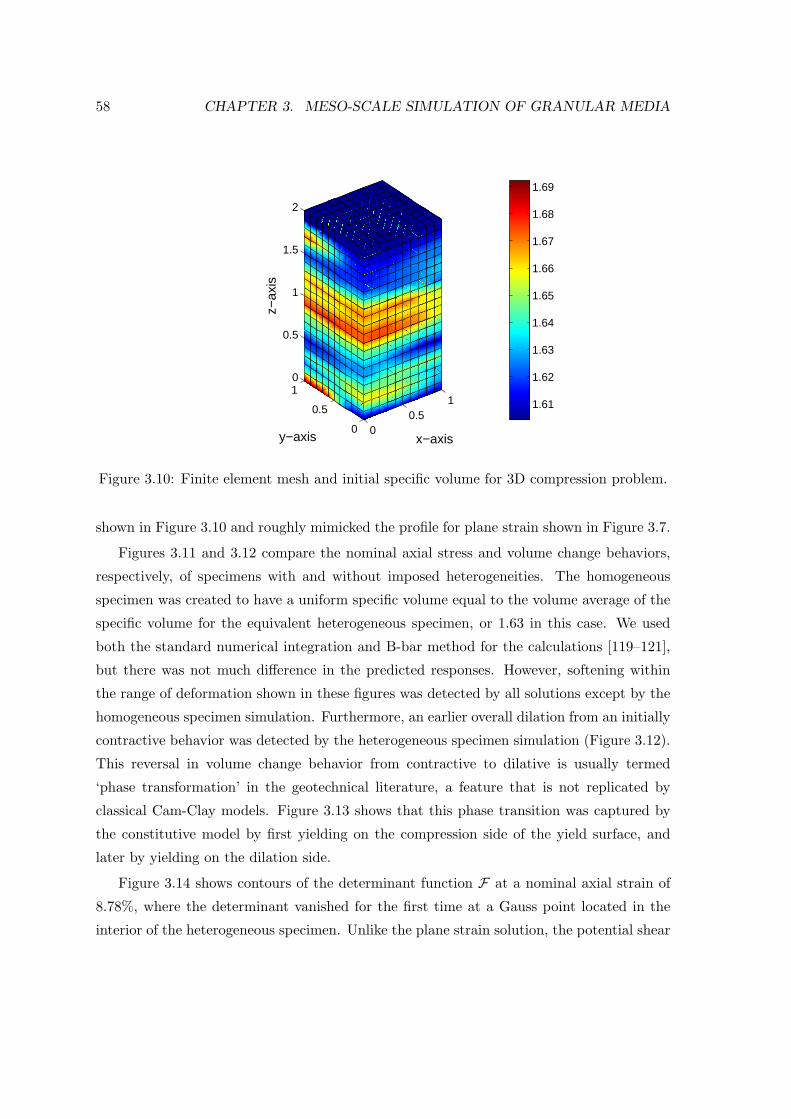
58 CHAPTER 3. MESO-SCALE SIMULATION OF GRANULAR MEDIA
00.5
1
0
0.5
10
0.5
1
1.5
2
x−axisy−axis
z−ax
is
1.61
1.62
1.63
1.64
1.65
1.66
1.67
1.68
1.69
Figure 3.10: Finite element mesh and initial specific volume for 3D compression problem.
shown in Figure 3.10 and roughly mimicked the profile for plane strain shown in Figure 3.7.
Figures 3.11 and 3.12 compare the nominal axial stress and volume change behaviors,
respectively, of specimens with and without imposed heterogeneities. The homogeneous
specimen was created to have a uniform specific volume equal to the volume average of the
specific volume for the equivalent heterogeneous specimen, or 1.63 in this case. We used
both the standard numerical integration and B-bar method for the calculations [119–121],
but there was not much difference in the predicted responses. However, softening within
the range of deformation shown in these figures was detected by all solutions except by the
homogeneous specimen simulation. Furthermore, an earlier overall dilation from an initially
contractive behavior was detected by the heterogeneous specimen simulation (Figure 3.12).
This reversal in volume change behavior from contractive to dilative is usually termed
‘phase transformation’ in the geotechnical literature, a feature that is not replicated by
classical Cam-Clay models. Figure 3.13 shows that this phase transition was captured by
the constitutive model by first yielding on the compression side of the yield surface, and
later by yielding on the dilation side.
Figure 3.14 shows contours of the determinant function F at a nominal axial strain of
8.78%, where the determinant vanished for the first time at a Gauss point located in the
interior of the heterogeneous specimen. Unlike the plane strain solution, the potential shear
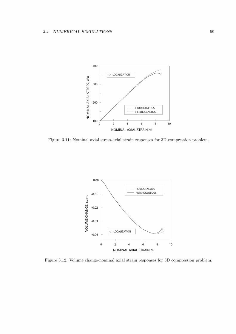
3.4. NUMERICAL SIMULATIONS 59
0100
2 4 6 8 10
200
300
400
NOMINAL AXIAL STRAIN, %
NO
MIN
AL
AX
IAL
ST
RE
SS
, k
Pa
HOMOGENEOUS
HETEROGENEOUS
LOCALIZATION
Figure 3.11: Nominal axial stress-axial strain responses for 3D compression problem.
0 2 4 6 8 10
NOMINAL AXIAL STRAIN, %
VO
LU
ME
CH
AN
GE
, c
u.m
.
HOMOGENEOUS
HETEROGENEOUS
LOCALIZATION
− 0.01
− 0.02
0.00
− 0.03
− 0.04
Figure 3.12: Volume change-nominal axial strain responses for 3D compression problem.

60 CHAPTER 3. MESO-SCALE SIMULATION OF GRANULAR MEDIA
−1200 −1000 −800 −600 −400 −200 00
100
200
300
400
500
600
MEAN NORMAL STRESS, kPa
DE
VIA
TO
RIC
ST
RE
SS
, kP
a
STRESS PATHYIELD SURFACE
Figure 3.13: Stress path for homogeneous specimen simulation with finite deformation.
band did not exhibit an X-pattern in this case. Instead, the solution predicted a well-defined
band extending across the specimen. Note that the horizontal slices shown in Figure 3.14b
have been rotated by 90 degrees on the horizontal plane relative to the orientation of the
solid volume shown in Figure 3.14a for optimal 3D visualization (red regions in Figure 3.14a
must be matched with red regions in Figure 3.14b, etc.). As for the homogeneous specimen,
the computation was carried out up to 15% nominal axial strain but the sample did not
localize.
Figure 3.15 shows contours of the deviatoric invariant of logarithmic stretches at the
point of initial localization. Again, the horizontal slices (Figure 3.15b) are 90 degrees rotated
relative to the solid volume (Figure 3.15a) for better visualization. Comparing Figures 3.14
and 3.15, the solutions clearly correlated regions in the specimen where the determinant
function vanished for the first time with regions where the deviatoric strains were most
intense (a ‘blue’ determinant region correlates with a ‘red’ deviatoric strain region, etc.).
In contrast, Figure 3.16 shows contours of the volumetric invariant of logarithmic stretches
resembling the initial specific volume profile of Figure 3.10. In general, these observations are
similar to those observed for the plane strain example. For completeness, Figure 3.17 shows
the deformed FE mesh for the heterogeneous sample at the instant of initial localization,
suggesting that the specimen moved laterally as well as twisted torsionally. Note once again

3.5. CLOSURE 61
0
0.5
1
0
0.5
1
0
0.5
1
1.5
x−axisy−axis
z−axis
0
0.5
1 0
0.5
1
0
0.5
1
1.5
y−axisx−axisz−axis
0.5
1
1.5
2
2.5
3
x 1010
(a) (b)
Figure 3.14: Determinant function at onset of localization.
that this non-uniform deformation was triggered by the imposed initial density variation
alone.
Finally, Figure 3.18 shows the convergence profiles of global Newton iterations for the
full 3D finite deformation simulation of a heterogeneous specimen with B-bar integration.
The iterations converged quadratically in all cases, suggesting optimal performance. We
emphasize that all of the results presented above only pertain to the prediction of when and
where a potential shear band will emerge. We have not pursued the simulations beyond
the point of bifurcation due to mesh sensitivity issues inherent in rate-independent classical
plasticity models in the post-localized regime. A host of regularization techniques either in
the constitutive description or finite element solution are available and should be used to
advance the solution to this regime.
3.5 Closure
We have presented a meso-scale finite element modeling approach for capturing deformation
and strain localization in dense granular materials using critical state plasticity theory
and nonlinear finite element analysis. This approach has been motivated in large part by

62 CHAPTER 3. MESO-SCALE SIMULATION OF GRANULAR MEDIA
0
0.5
1
0
0.5
1
0
0.5
1
1.5
x−axisy−axis
z−axis
0
0.5
1 0
0.5
1
0
0.5
1
1.5
y−axisx−axis
z−axis
0.03
0.04
0.05
0.06
0.07
0.08
0.09
0.1
0.11
0.12
(a) (b)
Figure 3.15: Deviatoric invariant of logarithmic stretches at onset of strain localization.
0
0.5
1
0
0.5
1
0
0.5
1
1.5
x−axisy−axis
z−axis
0
0.5
1 0
0.5
1
0
0.5
1
1.5
y−axisx−axis
z−axis
−0.024
−0.022
−0.02
−0.018
−0.016
−0.014
−0.012
−0.01
(a) (b)
Figure 3.16: Volumetric invariant of logarithmic stretches at onset of strain localization.

3.5. CLOSURE 63
x−axis
y−axis
z−ax
is
Figure 3.17: Deformed finite element mesh at onset of localization (deformation magnifiedby a factor of 3).
20
40
60
STEP NO.
ITERATION NUMBER
0 1 2 3 4 5 6 7
0
− 2
− 4
− 6
− 8
− 10
− 12
2
LOG
NO
RM
OF
RE
SID
UAL
Figure 3.18: Convergence profiles of global Newton iterations: finite deformation simulationof heterogeneous specimen with B-bar.

64 CHAPTER 3. MESO-SCALE SIMULATION OF GRANULAR MEDIA
recent trends in geotechnical laboratory testing allowing accurate quantitative measurement
of the spatial density variation in discrete granular materials. The meso-scale approach
provides a more realistic mathematical representation of imperfection; hence, it is expected
to provide a more thorough capture of the deformation and strain localization processes in
these materials. Potential extensions of the studies include a three-invariant enhancement
of the plasticity model and application of the model to unstructured random density fields
(in contrast to the structured density fields simulated in this paper). These aspects will be
reported upon in a future publication.
Acknowledgments
This work has been supported by National Science Foundation under Grant Nos. CMS-
0201317 and CMS-0324674 to Stanford University. We thank Professor Jack Baker of
Stanford University for his assistance in generating the initial specific volume profiles used
in the numerical examples, and Professor Amy Rechenmacher of USC for providing the
X-Ray CT image shown in Figure 3.1. We also thank the two anonymous reviewers for
their constructive reviews.

Chapter 4
Capturing strain localization in
dense sands with random density
This Chapter is published in: J.E. Andrade and R. I. Borja. Capturing strain localiza-
tion in dense sands with random density. International Journal for Numerical Methods in
Engineering, 2006. In press.
Abstract
This paper presents a three-invariant constitutive framework suitable for the numerical
analyses of localization instabilities in granular materials exhibiting unstructured random
density. A recently proposed elastoplastic model for sands based on critical state plasticity
is enhanced with the third stress invariant to capture the difference in the compressive and
extensional yield strengths commonly observed in geomaterials undergoing plastic deforma-
tion. The new three-invariant constitutive model, similar to its two-invariant predecessor,
is capable of accounting for meso-scale inhomogeneities as well as material and geometric
nonlinearities. Details regarding the numerical implementation of the model into a fully
nonlinear finite element framework are presented and a closed-form expression for the con-
sistent tangent operator, whose spectral form is used in the strain localization analyses,
is derived. An algorithm based on the spectral form of the so-called acoustic tensor is
proposed to search for the necessary conditions for deformation bands to develop. The
aforementioned framework is utilized in a series of boundary-value problems on dense sand
65

66 CHAPTER 4. STRAIN LOCALIZATION IN DENSE SANDS
specimens whose density fields are modeled as exponentially distributed unstructured ran-
dom fields to account for the effect of inhomogeneities at the meso-scale and the intrinsic
uncertainty associated with them.
4.1 Introduction
Shear bands in granular materials, characterized by thin zones of intense shearing, have been
a subject of considerable research interest since they impact many problems in the fields
of geoengineering and geoscience. In geoengineering, shear bands control the deformation
behavior and stability of earth structures such as dams, tunnels, excavations and founda-
tions. In geoscience, they are commonly associated with grain fracturing and grain size
reduction (termed “cataclasis” in the literature [43]) that are known to alter the strength
and transport properties of geological systems. Various experimental and theoretical studies
have thus attempted to analyze and describe the occurrence and patterns of shear bands in
granular materials such as soils and rocks.
In sand bodies, shear band formations are now investigated in the laboratory using
advanced testing techniques such as gamma-rays, stereophotogrammetry, and X-Ray Com-
puted Tomography (CT), see [80]. Along with the more traditional laboratory testing
procedures such as triaxial and simple shear testing, high-end testing provides an oppor-
tunity to view the specimen as an imperfect structure. For example, it is now possible
to measure quantitatively the density and displacement fields within the specimen with a
high degree of precision. Instead of viewing the entire specimen as a homogeneous element,
which has been traditionally done in the past, it is now possible to digitally measure and
quantify the properties and mechanical responses of an imperfect specimen on a finer scale.
Ironically, whereas development of very sophisticated constitutive models for element
testing has previously outpaced the development of laboratory testing capabilities support-
ing the demands of these complex models, the reverse is now true with the advent of high-end
precision laboratory testing. There is now a shortage of mathematical models that can ade-
quately capture the quantified heterogeneities in the properties and mechanical responses of
imperfect soil samples. This is because many of these sophisticated models are simply too
complex to be implemented efficiently into multi-purpose finite element codes, and so only
a handful of these models have been successful in finding their way into general-purpose
computer codes. Since heterogeneous samples require that their responses be analyzed as

4.1. INTRODUCTION 67
a boundary-value problem and not as an elemental point, many of these complex models
have to be reformulated first before they can be used for general-purpose boundary-value
problem simulations.
A promising approach to simulating material heterogeneity in specimens of discrete
granular materials such as sand bodies is through meso-scale modeling. By “meso-scale”
we mean a scale larger than a particle size but smaller than the specimen dimensions. We
do not wish to go to particle level at this point since there is currently a lack of testing
capabilities to capture all the particle information such as shapes, dimensions, and motion
of the individual particles throughout testing. In contrast, some of the high-end testing
techniques mentioned above, specifically the CT digital imaging technique, can very well be
combined with existing computer tools that permit an accurate quantification of material
heterogeneity in soil samples. Examples of such techniques include Digital Image Processing
(DIP) for quantifying the spatial density variation and Digital Image Correlation (DIC) for
tracking the motion of a group of particles contained in a “meso-element” having the size
of a pixel [83, 84].
From a modeling standpoint, a key variable that quantitatively describes material het-
erogeneity on a meso-scale level is density. Whereas it may be argued that other constitutive
variables such as strength and stiffness could also vary spatially within a soil sample, and
therefore they should also be considered as meso-variables, it is generally difficult if not
impossible to measure their spatial variation in a heterogeneous soil sample. In contrast,
DIP can be used to analyze pixel patterns provided by CT images to correlate the gray
level with density pattern in the individual pixels. Furthermore, strength and stiffness are
known to correlate strongly with density in soils, so it seems plausible to claim that density
is indeed a key measure of material heterogeneity.
Having chosen density as a key measure of material heterogeneity, we now consider a
constitutive model based on critical state plasticity theory that permits the specification
of spatial density variation within a soil sample. One such model, derived from the “Nor-
Sand” of Jefferies [2] and presented by Borja and Andrade [122], utilizes a variable called
“state parameter” ψ to describe the density of a meso-element relative to that at the critical
state line for the same effective mean normal stress [2, 75, 106]. Where the point lies below
the critical state line, ψ is negative (denser than critical), and where it lies above, ψ is
positive (looser than critical). Traditional Cam-Clay type models [65, 66, 72, 73, 104, 105],
68 CHAPTER 4. STRAIN LOCALIZATION IN DENSE SANDS
do not have the capability to independently prescribe the density (or void ratio) of a meso-
element, since, by prescribing the degree of overconsolidation [65] and the current state of
stress, one is bound to calculate a unique void ratio. By introducing the state parameter in
the constitutive description, the density (or other equivalent measures thereof, such as the
void ratio and specific volume) is effectively “detached” from the critical state line.
This paper moves one step further in refinement to the two-invariant model presented
by Borja and Andrade [122] in that we now also quantify the influence of the third stress
invariant in the constitutive description of meso-element behavior. Granular materials such
as soils are known to exhibit yield stresses in compression that are higher than those in
extension, so it only makes sense to include the third stress invariant in the constitutive
formulation. Furthermore, it has been shown that the third stress invariant does enhance
the onset of strain localization [111, 114], thus further motivating the present effort. For
the present paper we introduce the third stress invariant through Lode’s angle [123] and
employ a return mapping algorithm in principal elastic logarithmic stretches (within the
framework of multiplicative plasticity) to carry out the numerical integration in discrete
load steps.
Apart from the inclusion of the third stress invariant, the present paper also models the
effect of unstructured random density fields in the mathematical characterization of nearly
homogeneous soil samples at meso-scale. Borja and Andrade [122] have shown that a well
defined density structure, generated deterministically, could greatly impact the position of
the resulting shear band. However, in reality most laboratory testing procedures attempt
to generate as nearly uniform soil samples as possible. Thus the numerical simulations
presented in this paper focus on nearly homogeneous density fields, generated randomly
and without any preferred structure, to better capture reality. We show with extensive
numerical simulations that even with such minute perturbations in the density field a shear
band would still form even in cases where it would not form in perfectly homogeneous spec-
imens. Further, we show that different shear bands could form in each randomly generated
specimen, even with a very tight density distribution, affirming the common notion that
each physical specimen is unique.
Evaluation of the consistent tangent operator (CTO) is critical for the success of a
nonlinear iterative algorithm based on Newton’s method, and in this paper we derive such
tangent operator in spectral form based on Lie derivatives. Quite recently, Borja [114]
has shown that such operator can also be used in lieu of the constitutive tangent operator

4.2. CONSTITUTIVE ASSUMPTIONS 69
for strain localization analysis, so the CTO serves a dual role in the present numerical
simulations. All simulations presented in this paper have been conducted in the 3D finite
deformation regime, including the calculation of the minimum values of the localization
function for shear band analysis [64]. For the latter analysis we also present an algorithm
for a 3D search in spectral directions.
As for notations and symbols used in this paper, bold-faced letters denote tensors and
vectors; the symbol ‘·’ denotes an inner product of two vectors (e.g. a ·b = aibi), or a single
contraction of adjacent indices of two tensors (e.g. c · d = cijdjk); the symbol ‘:’ denotes
an inner product of two second-order tensors (e.g. c : d = cijdij), or a double contraction
of adjacent indices of tensors of rank two and higher (e.g. C : ǫe = Cijklǫekl); the symbol
‘⊗’ denotes a juxtaposition, e.g., (a ⊗ b)ij = aibj . Finally, for any symmetric second order
tensors α and β, (α ⊗ β)ijkl = αijβkl, (α ⊕ β)ijkl = βikαjl, and (α ⊖ β)ijkl = αilβjk.
4.2 Constitutive assumptions
In this section we present a three-invariant enhancement of the critical state plasticity
model by Borja and Andrade [122]. As mentioned in the Introduction, geomaterials exhibit
a higher yield strength in compression than in extension, so the addition of the third stress
invariant is critical for modeling the behavior of geomaterials more realistically. Further, the
hyperelastoplastic model hinges on the well established assumption that the deformation
gradient tensor can be decomposed multiplicatively into elastic and plastic parts [115],
F = F e · F p, (4.2.1)
where F e and F p are defined as the elastic and plastic deformation gradient, respectively.
4.2.1 The hyperelastic model
Consider an isotropic hyperelastic response entailing a strain energy that is a function of
either the elastic right Cauchy-Green deformation tensor Ce or the left Cauchy-Green tensor
be i.e., Ψ = Ψ (Ce) = Ψ (be) [30, 124], where
Ce := F e t · F e and be := F e · F e t. (4.2.2)

70 CHAPTER 4. STRAIN LOCALIZATION IN DENSE SANDS
The principal elastic stretches emanate from F e · Na = λean
a (no sum), where λea for
a = 1, 2, 3 are the principal elastic stretches in the corresponding principal directions Na
and na in the intermediate and current configuration, respectively. We recall the well known
spectral decomposition,
be =3∑
a=1
λe 2a na ⊗ na. (4.2.3)
The elastic region is assumed to be governed by the isotropic strain energy function
proposed in [1] and utilized in modeling of granular bodies in [66, 125]
Ψ (εev, εes) = Ψ (εev) +
3
2µeεe 2
s , (4.2.4)
where
Ψ (εev) = −p0κ expω, ω = −εev − εev 0
κ, µe = µ0 +
α0
κΨ (εev) . (4.2.5)
The independent variables are the volumetric and deviatoric invariants of the elastic loga-
rithmic stretch tensor, respectively,
εev = εe1 + εe2 + εe3 and εes =1
3
√2[(εe1 − εe2)
2 + (εe2 − εe3)2 + (εe3 − εe1)
2], (4.2.6)
where εea ≡ lnλea. Hence, the strain energy function is an invariant function of the elastic
deformations. The Kirchhoff stress tensor τ is coaxial with the deformation tensor be and
defined such that
τ = 2∂Ψ
∂be · be. (4.2.7)
The above hyperelastic model produces pressure-dependent elastic bulk and shear moduli,
a feature commonly observed in the laboratory. The elastic constants necessary for a full
description of the elasticity are the reference strain εev 0 and the reference pressure p0 of
the elastic compression curve, as well as the compressibility index κ. The model produces
coupled volumetric and deviatoric responses in the case α0 6= 0 for which µe is a nonlinear
function of the volumetric deformations. Otherwise, for α0 = 0 the responses are decoupled
and the shear modulus µe ≡ µ0 is constant.

4.2. CONSTITUTIVE ASSUMPTIONS 71
4.2.2 Yield surface, plastic potential, their derivatives and the flow rule
We define the three invariants of the Kirchhoff stress tensor as
p =1
3tr τ , q =
√3
2‖ξ‖, 1√
6cos 3θ =
tr ξ3
χ3≡ y, (4.2.8)
where ξ = τ − p1 is the deviatoric component of the stress tensor τ , and χ =√
tr ξ2. The
quantity p is called the mean normal stress and is assumed negative throughout. Further, θ
is the Lode’s angle whose values range from 0 ≤ θ ≤ π/3; it defines an angle on a deviatoric
plane emanating from a tension corner.
From these three stress invariants we construct a yield surface of the form
F (τ , πi) = F (p, q, θ, πi) = ζ (θ) q + pη (p, πi) (4.2.9)
where
η =
M [1 + ln (πi/p)] if N = 0
M/N[1 − (1 −N) (p/πi)
N/(1−N)]
if N > 0.(4.2.10)
The image stress πi < 0 controls the size of the yield surface; it is defined such that the
stress ratio η = −ζq/p = M when p = πi. Note the subscript ‘i’ stands for image and should
not be confused with index notation. The parameter N ≥ 0 determines the curvature of
the yield surface on a meridian plane and it typically has a value less than or equal to 0.4
for sands [2]. Lode’s angle θ plays the role of the third stress invariant modifying the shape
of the yield surface on a deviatoric plane through the function ζ = ζ (θ). Many forms for
the function ζ (θ) have been proposed in the literature (see [126] for a historical survey).
Here we adopt the form proposed by Gudehus in [127] and Argyris et al. in [128], namely,
ζ (θ, ρ) =(1 + ρ) + (1 − ρ) cos 3θ
2ρ(4.2.11)
where ρ is a constant parameter called ellipticity. The above function is only convex for
7/9 ≤ ρ ≤ 1 [129] and satisfies the boundary conditions: (a) ζ = 1/ρ when θ = 0 i.e., tension
corner; and (b) ζ = 1 when θ = π/3 i.e., compression corner. A typical three-invariant yield
surface of the form presented above for ρ = 0.78 is shown in Figure 1. It can be seen from
this figure that the yield surface exhibits a greater yield strength under compression than
under extension.

72 CHAPTER 4. STRAIN LOCALIZATION IN DENSE SANDS
t =t =t1 2 3
t1 t2
t3
(a) (b)
Figure 4.1: Three-invariant yield surface in Kirchhoff stress space for ρ = 0.78. (a) Cross-section on deviatoric plane, dashed line represents two-invariant counterpart for comparisonand (b) three-dimensinal view.
Additionally, to underscore the fact that the formulation presented herein is general and
independent of the choice of the shape function ζ (θ, ρ), in some of our numerical examples,
we will also utilize the form proposed by Willam and Warnke [130] i.e.,
ζ (θ, ρ) =4(1 − ρ2
)cos2 θ + (2ρ− 1)2
2 (1 − ρ2) cos θ + (2ρ− 1) [4 (1 − ρ2) cos2 θ + 5ρ2 − 4ρ]1/2. (4.2.12)
This function is smooth and convex in the range 1/2 ≤ ρ ≤ 1, and has the same boundary
conditions than the shape function in (4.2.11).
Similar to the yield surface, we can postulate a plastic potential function of the form
Q (τ , πi) = Q (p, q, θ, πi) = ζ (θ) q + pη (p, πi) (4.2.13)
with
η =
M [1 + ln (πi/p)] if N = 0
M/N[1 −
(1 −N
)(p/πi)
N/(1−N)]
if N > 0.(4.2.14)
When πi = πi, N = N and ζ = ζ, plastic flow is associative; otherwise, it is nonassociative
in both the volumetric and deviatoric sense. The material parameter N controls the amount
of volumetric nonassociativity, whereas the shape function ζ = ζ (θ, ρ) plays a similar role
than that used in the yield surface, but the ellipticity ρ can be different from ρ, hence

4.2. CONSTITUTIVE ASSUMPTIONS 73
introducing deviatoric nonassociativity. We note in passing that the plastic potential in
(4.2.13) is essentially that proposed by Jefferies in [2] for ζ = 1.
Recall the multiplicative decomposition of the deformation gradient tensor in (4.2.1),
which leads to an additive decomposition of the velocity gradient l,
l = le + lp ⇒ d = de + dp, (4.2.15)
where d ≡ sym l, de ≡ sym le, and dp ≡ sym lp. Neglecting the plastic spin ωp (see [118]
for significance and consequences), we write the flow rule as
dp = λq, (4.2.16)
where λ is the so-called consistency parameter, and q := ∂Q/∂τ . Adopting the spectral
approach [111], we recast the above gradient as
q =∂Q
∂τ=
3∑
a=1
∂Q
∂τama =
3∑
a=1
qama (4.2.17)
where ma := na ⊗na, and the vectors na for a = 1, 2, 3, are the principal directions of the
stress tensor τ , i.e., τ · na = τana, with principal stresses τa for a = 1, 2, 3. Note that the
stress tensor τ and the elastic left Cauchy-Green deformation tensor be are coaxial due to
the isotropy assumption made in Section 4.2.1 above. The spectral decomposition of the
flow rule is consequently a by-product of the coaxiality of the tensors τ and be as well as
the fact that Q is an isotropic function of the stress tensor and hence its gradient and the
stress tensor are also coaxial. It is then useful to expand qa such that
qa =∂Q
∂p
∂p
∂τa+∂Q
∂q
∂q
∂τa+∂Q
∂θ
∂θ
∂τa(4.2.18)
where we can easily show that
∂p
∂τa=
1
3δa,
∂q
∂τa=
√3
2
ξaχ
≡√
3
2na,
∂θ
∂τa≡ θa = −
(2√6
csc 3θ
)ya, (4.2.19)
where δa = 1, and ξa for a = 1, 2, 3 are the eigenvalues of the deviatoric stress tensor ξ.
Additionally,
ya =∂y
∂τa= 3
ξ2aχ3
− 3tr(ξ3)ξa
χ5− δaχ
, (4.2.20)

74 CHAPTER 4. STRAIN LOCALIZATION IN DENSE SANDS
which we use to write qa in more compact form
qa =1
3∂pQδa +
√3
2∂qQna + ∂θQθa. (4.2.21)
From equations (4.2.9) and (4.2.13), we obtain
∂Q
∂p= β
∂F
∂p,
∂Q
∂q= ζ,
∂Q
∂θ= ζ
′q, (4.2.22)
where we have used the volumetric nonassociativity parameter
β := (1 −N) /(1 −N
). Thus,
qa =1
3β∂pFδa +
√3
2∂qQna + ∂θQθa, (4.2.23)
from where we clearly see the volumetric and deviatoric nonassociativity in the plastic flow.
Using the above expression for the yield surface, we calculate the derivatives
∂F
∂p=η −M
1 −N,
∂F
∂q= ζ,
∂F
∂θ= ζ ′q. (4.2.24)
It is now convenient to evaluate the second derivative of the plastic potential with respect
to the stress tensor, as it will be used in the numerical implementation of the model. Here,
we exploit the uncoupling between the volumetric and deviatoric terms in F and write
qab =1
9β∂2
ppFδaδb +
√3
2∂qQnab + ∂θQθab + ∂2
θθQθaθb
+
√3
2∂2qθQ (naθb + θanb) , (4.2.25)
where, from equations (4.2.24) and (4.2.22), we get
∂2ppF = − M
1 −N
1
p
(p
pi
)N/(1−N)
, ∂2θθQ = ζ
′′q, ∂2
qθQ = ζ′. (4.2.26)
Furthermore, from equations (4.2.19)2,3 we get, respectively,
nab =1
χ
(δab −
1
3δaδb − nanb
)and θab = −
(2√6
csc 3θ
)yab − (3 cot 3θ) θaθb,
(4.2.27)

4.2. CONSTITUTIVE ASSUMPTIONS 75
with
yab = 6ξaδabχ3
− 3tr ξ3
χ5
(δab −
1
3δaδb − 5
ξaξbχ2
)
+1
χ3(δaξb + ξaδb) −
9
χ5
(ξaξ
2b + ξ2aξb
)(no sum). (4.2.28)
Reduced dissipation inequality: the second law of thermodynamics
For perfect plasticity, the reduced dissipation inequality requires the stresses to perform
nonnegative plastic incremental work [112], i.e.,
Dp ≡ τ : dp = λτ : q = λ3∑
a=1
τaqa ≥ 0. (4.2.29)
Realizing that∑3
a=1 τaθa = 0, we can write
Dp = λ (p∂pQ+ q∂qQ) = −λp(M − η
1 −N+ η
)≥ 0, (4.2.30)
where we have exploited the fact that at yield F = Q = 0. Since −λp ≥ 0 and 1 −N > 0,
we require −Nη + M ≥ 0. Now, for a stress point on the yield surface, the relationship
η/ζ = η/ζ holds, hence,
Dp ≥ 0 ⇒ −MN
N
ζ
ζ
[1 − (1 −N)
(p
πi
)N/(1−N)]
+M ≥ 0. (4.2.31)
It can be seen that the function inside the square brackets is a monotonically decreasing
function and always less than unity for p ∈ [πc, 0], where πc = πi/ (1 −N)(1−N)/N is the
preconsolidation pressure. Therefore, since M > 0 as it is a physical parameter, we get the
condition(N ζ
)/ (Nζ) ≤ 1, which is satisfied at all times if
N ≤ N and ζ ≤ ζ. (4.2.32)
The first condition was already derived by the authors in [122] in the context of two-
invariant plasticity, whereas the second condition is a by-product of the third invariant.
Both restrictions derived above can be linked to the angle of friction and angle of dilation
as N ≤ N implies lower dilatancy than that achieved from a volumetric associative flow

76 CHAPTER 4. STRAIN LOCALIZATION IN DENSE SANDS
rule. On the other hand, it is easy to show that the second condition requires ρ ≤ ρ, and
since
ρ ≡ 3 − sinφc3 + sinφc
and ρ ≡ 3 − sinψc3 + sinψc
, (4.2.33)
where φc is the angle of internal friction at critical and ψc is the dilatancy angle at critical,
it follows that
ψc ≤ φc, (4.2.34)
which is very much consistent with thermodynamic conditions found for Mohr-
Coulomb or Drucker-Prager materials and experimental observations in geomaterials, see
[110, 111] for further elaboration.
Remark 3. Experimental evidence in granular materials seems to suggest deviatoric nonas-
sociativity in these materials is not pronounced. Lade and Duncan [8] have shown that, for
dense sands, the plastic strain rates are perpendicular to the yield surface on a deviatoric
plane. Nevertheless, the formulation presented above is general and allows for deviatoric
and volumetric nonassociativity.
4.2.3 Maximum plastic dilatancy, hardening law and the consistency con-
dition
We recall the definitions for the volumetric and deviatoric plastic strain rate invariants,
respectively,
εpv = trdp and εps =
√2
3‖dp − 1/3εpv1‖ . (4.2.35)
Using the definitions above and equations (4.2.16)-(4.2.17), and (4.2.21) we get
εpv = λ3∑
a=1
qa and εps = λ
√√√√2
3
3∑
a=1
q2a, (4.2.36)
where we have∑3
a=1 qa = ∂pQ, and qa = qa − 1/3∂pQδa. Hence,
εpv = λβ∂pF and εps = λ
√2
3Ω (q, θ) , (4.2.37)
with
Ω (τ ) = Ω (q, θ) =
√3
2(∂qQ)2 + (∂θQ)2
[θ21 + θ2
2 + θ23
]. (4.2.38)

4.2. CONSTITUTIVE ASSUMPTIONS 77
Now, we recall the definition of plastic dilatancy
D :=εpvεps
=
√3
2β∂pF
Ω, (4.2.39)
which we can use to obtain the maximum dilatancy and thereby maximum stress ratio η∗
such that
D∗ = αψi =
√3
2βη∗ −M
(1 −N) Ω. (4.2.40)
After rearranging, we get η∗ =√
2/3αψi(1 − N)Ω + M , with α = βα and α ≈ −3.5 for
sands. Recall the maximum plastic dilatancy is used to limit the amount of dilation in a sand
specimen on the ‘wet’ side of the critical state line. As in the original model proposed by
Been and Jefferies in [106] and Jefferies in [2], the maximum dilatancy is obtained through
an empirical relation with the state parameter ψi, which is a distance between the specific
volume of the sample and the specific volume at critical at the image pressure i.e.,
ψi = v − vc0 + λ ln (−πi) , (4.2.41)
where v is the specific volume, vc0 is the reference specific volume at unit pressure, and λ is
the plastic compressibility index. All of these parameters emanate from the so-called critical
state theory which postulates the existence of the critical state line. Inserting the above
result into equation (4.2.10) and solving for the corresponding limiting image pressure we
get, cf. [122],
π∗ip
=
exp(√
2/3α/MψiΩ)
if N = N = 0,(1 −
√2/3αψiΩN/M
)(N−1)/Nif 0 ≤ N ≤ N 6= 0.
(4.2.42)
Recall the hardening law, which relates the image pressure with the state of stress, the state
parameter ψi, and the deviatoric component of plastic flow, i.e.,
πi = h (π∗i − πi) εps =
√2
3hλ (π∗i − πi) Ω, (4.2.43)
where h is a constant material property, to be calibrated in the finite deformation regime.

78 CHAPTER 4. STRAIN LOCALIZATION IN DENSE SANDS
Finally, for elastoplasticity the consistency condition necessitates
F = f : τ −Hλ = 0, λ > 0, (4.2.44)
where f := ∂F/∂τ and H is the so-called hardening modulus defined as
H = − 1
λ
∂F
∂πiπi = − 1
λ
(p
πi
)1/(1−N)
Mπi. (4.2.45)
Since p/πi > 0, the sign of the hardening modulus is governed by the sign of the image
pressure rate: H > 0 if πi < 0 (expansion of the yield surface, hardening), H < 0 if πi > 0
(contraction of the yield surface, softening), and H = 0 if πi = 0 (perfect plasticity).
Remark 4. The continuum formulation presented above is a generalization of that presented
in [122]. In fact, when ζ = ζ = 1 ∀ θ ∈ [0, π/3], all derivatives of Q with respect to θ drop
out, and with Ω =√
3/2 we recover the original two-invariant version of the model.
4.3 Numerical implementation
We perform a numerical stress point integration based on the product formula algorithm
similar to that proposed by Simo in [117]. However, here we perform the return mapping in
the elastic principal stretch directions to accommodate for nonlinear elasticity. Note that
the algorithm provides a closed-form expression for the consistent tangent operator (CTO).
The numerical implementation developed below is summarized in Tables 4.1 and 4.2. Table
4.1 presents a summary of the evolution equations used in the local return mapping, whose
recipe is presented in turn in Table 4.2.
4.3.1 Local return mapping algorithm
Recall the definition of the elastic left Cauchy-Green deformation tensor given in equation
(4.2.2)2. From this expression we obtain the trial elastic left Cauchy-Green deformation
tensor at time station tn+1 by freezing plastic flow i.e.,
be tr ≡ b = fn+1 · ben · f t
n+1, fn+1 =∂xn+1
∂xn. (4.3.1)

4.3. NUMERICAL IMPLEMENTATION 79
Table 4.1: Summary of rate equations in three-invariant elastoplastic model for sands.
1. Additive velocity gradient: l = le + lp =⇒ d = de + dp
2. Hyperelastic rate equations: Lv (τ ) = ce : de;ce = 4be · ∂Ψ/ (∂be ⊗ ∂be) · be
3. Nonassociative flow rule: dp = sym lp = λq;ωp = skw lp = 0
4. State parameter: ψi = v + λπi/πi
5. Hardening law: πi =√
2/3hλ (π∗i − πi)Ω
6. Consistency condition: f : τ −Hλ = 0
7. Kuhn-Tucker optimality conditions: λ ≥ 0, F ≤ 0, λF = 0
Using the results presented in [117], the trial elastic deformation tensor can be related to
the elastic deformation tensor via the exponential approximation
be = exp (−2∆λq) · b, (4.3.2)
hence, εea = εe tra − ∆λqa and where εe tr
a ≡ εa for a = 1, 2, 3. From these results in principal
logarithmic stretches and utilizing the yield criterion, we formulate the residual vector
[111, 122, 131],
r (x) =
εe1 − εe tr1 + ∆λq1
εe2 − εe tr2 + ∆λq2
εe3 − εe tr3 + ∆λq3
F
with x =
εe1
εe2
εe3
∆λ
(4.3.3)

80 CHAPTER 4. STRAIN LOCALIZATION IN DENSE SANDS
Table 4.2: Return mapping algorithm for three-invariant elastoplastic model for sands.
1. Elastic deformation predictor: b = fn+1 · ben · f t
n+1
2. Elastic stress predictor: τ tr = 2∂Ψ/∂b · b; πtri = πi,n
3. Check if yielding: F(τ tr, πtr
i
)≥ 0?
No, set be = be tr ≡ b; τ = τ tr; πi = πtri and exit
4. Yes, initialize ∆λ = 0, build residual r (x) and iterate for x (steps 5-8)
5. Spectral decomposition: b =∑3
a=1 λ2am
a
6. Plastic corrector in principal logarithmic stretches: εea = lnλea;
εa ≡ εe tra = ln λa; εea = εe tr
a − ∆λqa; τa = ∂Ψ/∂εea for a = 1, 2, 3
7. Update plastic internal variable πi:
(a) Total deformation gradient: F = fn+1 · F n
(b) Specific volume: v = v0 detF = v0J
(c) Initialize πi = πi,n and iterate for πi (steps 7d-f)
(d) State parameter: ψi = v − vc0 + λ ln (−πi)
(e) Limit hardening plastic variable:
π∗i = p×
exp(√
2/3α/MψiΩ)
if N = N = 0,(1 −
√2/3αψiΩN/M
)(N−1)/Nif 0 ≤ N ≤ N 6= 0.
(f) Plastic internal variable: πi = πi,n +√
23h∆λ (π∗i − πi)Ω
8. Discrete consistency condition: F (p, q, θ, πi) = 0
9. Spectral resolution: be =∑3
a=1 λe 2a ma

4.3. NUMERICAL IMPLEMENTATION 81
as the vector of local unknowns. The Newton-Raphson scheme necessitates the Jacobian
r′ (x) =
1 + ∆λ∂q1/∂εe1 ∆λ∂q1/∂ε
e2 ∆λ∂q1/∂ε
e3 q1 + ∆λ∂q1/∂∆λ
∆λ∂q2/∂εe1 1 + ∆λ∂q2/∂ε
e2 ∆λ∂q2/∂ε
e3 q2 + ∆λ∂q2/∂∆λ
∆λ∂q3/∂εe1 ∆λ∂q3/∂ε
e2 1 + ∆λ∂q3/∂ε
e3 q3 + ∆λ∂q3/∂∆λ
∂F/∂εe1 ∂F/∂εe2 ∂F/∂εe3 ∂F/∂∆λ
.
(4.3.4)
The local tangent operator is fully defined once the quantities ∂qa/∂εeb, ∂qa/∂∆λ, ∂F/∂εea
for a, b = 1, 2, 3, and ∂F/∂∆λ are thoroughly computed. We compute these essential
derivatives in what follows.
Let us start by calculating the gradient
∂qa∂εeb
= qacaecb +
∂qa∂πi
∂πi
∂εeb, (4.3.5)
where aeab := ∂τa/∂ε
ea is the elastic continuum tangent operator in principal directions.
Also, we have
∂qa∂πi
=1
3β∂2F
∂p∂πiδa,
∂2F
∂p∂πi=
1
1 −N
M
p
(p
πi
) 11−N
. (4.3.6)
The last term of equation (4.3.5) is furnished by the hardening law, which we recall from
equation (4.2.43) and then integrate with a Backward Euler scheme to get
πi = πi,n +
√2
3h∆λ (π∗i − πi) Ω, (4.3.7)
where πi,n is the converged value of the image pressure at the previous time step tn. There-
fore,
(1 +
√2
3h∆λΩ
)∂πi
∂εeb=
√2
3h∆λ
[(∂π∗i∂τa
aeab +
∂π∗i∂ψi
∂ψi
∂εeb
)Ω + (π∗i − πi)Ωaa
eab
], (4.3.8)
where we have
∂π∗i∂τa
=1
3
π∗ipδa + (1 −N)
π∗iM −
√2/3αψiΩN
√2
3αψiΩa (4.3.9)
and
Ωa =1
Ω
[3
2ζ ζ
′θa + ζ
′q(ζ′′θaq + ζ
′√3/2na
)θ2cδc +
(ζ′q)2θcθca
]. (4.3.10)

82 CHAPTER 4. STRAIN LOCALIZATION IN DENSE SANDS
Finally, recalling the definition of ψi we get
∂π∗i∂ψi
=
√2
3αΩ(1 −N)
π∗iM −
√2/3αψiΩN
and∂ψi
∂εeb=λ
πi
∂πi
∂εeb. (4.3.11)
Therefore,
∂πi
∂εeb= c−1
√2
3h∆λ
[Ω∂π∗i∂τa
+ (π∗i − πi) Ωa
]aeab, (4.3.12)
where c = 1 +√
2/3h∆λΩ(1 − λ/πi∂π∗i /∂ψi).
It is only left for us to evaluate the derivatives ∂qa/∂∆λ, ∂F/∂εeb, and ∂F/∂∆λ. By the
chain rule, we have
∂qa∂∆λ
=∂qa∂πi
c−1
√2
3hΩ(π∗i − πi)
︸ ︷︷ ︸∂πi/∂∆λ
. (4.3.13)
Finally, we compute
∂F
∂εeb= faa
eab +
∂F
∂πi
∂πi
∂εeband
∂F
∂∆λ=∂F
∂πi
∂πi
∂∆λ, (4.3.14)
where
fa ≡∂F
∂τa=
1
3∂pFδa +
√3
2∂qFna + ∂θFθa and
∂F
∂πi= M
(p
πi
)1/(1−N)
. (4.3.15)
In addition to the above local iterative scheme, one sub-local scheme is necessary to
solve for πi as it is a nonlinear function of the state of stress, and the state parameter ψi.
This is easily accomplished by introducing the scalar residual
r (πi) = πi − πi,n −√
2
3h∆λ (π∗i − πi) Ω, (4.3.16)
with the scalar tangent operator
r′ (πi) = 1 +
√2
3h∆λΩ
(1 − λ
πi
∂π∗i∂ψi
). (4.3.17)
Once the sub-local loop is finished and a value for πi is obtained, then ψi and π∗i can be
evaluated and the solution algorithm can proceed to the local Newton-Raphson scheme
presented above.

4.3. NUMERICAL IMPLEMENTATION 83
4.3.2 Consistent tangent in principal directions
Let us start by deriving the elastic tangent in principal directions aeab. Recall the hyperelastic
formulation presented in subsection 4.2.1. We have the strain energy function Ψ (εev, εes) from
which the Kirchhoff stress tensor is obtained such that
τa = 2∂Ψ
∂λe 2a
λe 2a =
∂Ψ
∂εea=
1
3pδa +
√2
3qna (no sum), (4.3.18)
where we have used the definitions p = ∂Ψ/∂εev and q = ∂Ψ/∂εes . Hence,
aeab = Keδaδb + 2µe
(δab −
1
3δaδb
)+
√2
3de (δanb + naδb) , (4.3.19)
where Ke := ∂p/∂εev is the elastic bulk modulus, 3µe := ∂q/∂εes where µe is the elastic shear
modulus, and de := ∂2Ψ/(∂εev∂εes).
Now, let us define aepab := ∂τa/∂εb as the consistent tangent in principal directions,
which we can evaluate with the help of the converged local residual vector via the chain
rule. Specifically,
aepab = ae
acapcb with ap
cb ≡∂εec∂εb
. (4.3.20)
We can then recall the converged local residual vector r (x) = 0 and by the chain rule
obtain∂xi∂εa
= −bij∂rj∂εa
∣∣∣∣x
, (4.3.21)
where b := [r′]−1 and therefore
apab = bac
(δcb − ∆λ
∂qc∂εb
∣∣∣∣x
)− ba4
∂F
∂εb
∣∣∣∣x
for a, b, c = 1, 2, 3. (4.3.22)
We also have∂qa∂εb
∣∣∣∣x
=∂qa∂πi
∂πi
∂εb
∣∣∣∣x
and∂F
∂εb
∣∣∣∣x
=∂F
∂πi
∂πi
∂εb
∣∣∣∣x
, (4.3.23)
where∂πi
∂εa
∣∣∣∣x
= c−1
√2
3h∆λΩv
∂π∗i∂ψi
δa. (4.3.24)
We note that in the special case of pure elasticity, the tangent apab ≡ δab and thus, aep
ab ≡ aeab.
It will be shown in the next section, that the consistent tangent in principal directions
contributes to the global consistent tangent operator, which for this particular class of

84 CHAPTER 4. STRAIN LOCALIZATION IN DENSE SANDS
return mapping algorithm can be obtained in closed-form.
4.4 Consistent tangent operators in spectral form based on
Lie derivatives
It is generally recognized that a consistent linearization of the so-called weak form of
balance of linear momentum is critical for optimal performance of an iterative algorithm
[124, 132, 133]. In particular, in the presence of nonlinear kinematics the concept of direc-
tional derivatives plays a key role in the linearization process. We proceed to developing
the CTO for the case of elastoplasticity. For the elastoplastic formulation, isotropy (i.e.,
Ψ = Ψ (λe1, λ
e2, λ
e3)) furnishes a connection between the elastic and trial kinematical quanti-
ties and consequently, it is a crucial component in our developments. The result hinges on
two main results.
Proposition 1. The Kirchhoff stress tensor can be obtained using the trial elastic left
Cauchy-Green deformation tensor be tr ≡ b := F · F t, i.e.,
τ = 2∂Ψ
∂b· b, (4.4.1)
where F e tr ≡ F =∑3
a=1 λana ⊗ Na is the trial elastic deformation gradient.
Proof. By definition,
τ = 2∂Ψ (be)
∂be · be. (4.4.2)
We also know that we can decompose b and be spectrally and get, respectively
b =3∑
a=1
λ2am
a and be =3∑
a=1
λe 2a ma, (4.4.3)
where we note the fact that the tensors b and be have the same eigenvectors, a by-product
of the return mapping algorithm. Then we use equations (4.4.2) and (4.4.3) along with the
chain rule and write
τ = 2
3∑
a=1
∂Ψ
∂λ2a
∂λ2a
∂λe 2a
λe 2a ma = 2
3∑
a=1
∂Ψ
∂λ2a
λ2a
λe 2a
λe 2a ma = 2
∂Ψ
∂b· b, (4.4.4)

4.4. CONSISTENT TANGENT OPERATORS 85
where we have exploited the algorithmic relationship between λea and λa (cf. equation
(4.5,b) in [117]) and the isotropy of the strain-energy function.
Proposition 2. Define the trial elastic right Cauchy-Green deformation tensor C := Ft ·
F =∑3
a=1 λ2aM
a, then
τ = 2∂Ψ
∂b· b = 2F · ∂Ψ
∂C︸︷︷︸:=1/2S
·F t= F · S · F t
. (4.4.5)
Proof. This is a standard result in continuum mechanics, but we will prove it here for
completeness. We start by taking the time derivative of the strain-energy function
˙Ψ =∂Ψ
∂b:˙b =
∂Ψ
∂C: ˙C
= 2
[∂Ψ
∂b· F]
: ˙F = 2
[F · ∂Ψ
∂C
]: ˙F , (4.4.6)
where we have exploited the symmetries of b and C, the isotropy of Ψ , and the chain
rule. Consequently, since the expression above must hold for all F , we conclude ∂Ψ/∂b =
F · ∂Ψ/∂C · F−1, from where equation (4.4.5) follows.
With equations (4.4.1) and (4.4.5), it is then easy to obtain a closed form expression
for the CTO by utilizing the spectral decomposition approach along with the relationship
between the material time derivative and the Lie derivative of the Kirchhoff stress tensor.
We start by taking the material time derivative of the Kirchhoff stress tensor
τ =d
dt
(F · S · F t
)
τ = ˙F · S · F t
+ F · S · ˙F t + F · ∂S
∂C︸︷︷︸:=A
: ˙C · F t
. (4.4.7)
It is then necessary to explicate all three terms above. We recall F = F · F p−1n and thus
˙F = F · F p−1
n = l · F , where F pn is the plastic deformation gradient at time tn. Using this
result, we can calculate
˙C = F
t · l · F + Ft · lt · F = 2F
t · d · F . (4.4.8)

86 CHAPTER 4. STRAIN LOCALIZATION IN DENSE SANDS
It is now possible to rewrite equation (4.4.7) as
τ = l · τ + τ · lt + c : d (4.4.9)
where we identify Lv (τ ) = c : d and
cijkl = 2FiI FjJ FkK FlLAIJKL. (4.4.10)
It is clear that since Ψ = Ψ(λ1, λ2, λ3
), then it follows that S =
∑3a=1 SaM
a and C =∑3
a=1 λ2aM
a are coaxial and consequently
A =3∑
a=1
3∑
b=1
∂Sa
∂λ2b
Ma ⊗ M b +1
2
3∑
a=1
∑
b 6=a
Sb − Sa
λ2b − λ2
a
(Mab ⊗ Mab + Mab ⊗ M ba
)(4.4.11)
and therefore, by pushing A forward with equation (4.4.10) and using the fact that λ2aSa =
τa we obtain
c =3∑
a=1
3∑
b=1
(aepab − 2τaδab
)︸ ︷︷ ︸
:=cab
ma ⊗ mb +3∑
a=1
∑
b 6=a
τbλ2a − τaλ
2b
λ2b − λ2
a︸ ︷︷ ︸:=γab
(mab ⊗ mab + mab ⊗ mba
)
(4.4.12)
where aepab := ∂τa/∂εb, εb := ln λb, and where Ma := Na⊗Na, Mab := Na⊗N b and mab :=
na⊗nb. We observe from equation (4.4.12) that the CTO possesses minor symmetries but
lacks major symmetry if aepab 6= aep
ba, which is certainly the case for non-associative plasticity
or when the integration algorithm destroys the symmetry of the tangent operator [66, 134].
4.5 Search algorithm in principal stress space
Consider the expression for the total tangent operator i.e., aep = cep + τ ⊕ 1, where the
elastoplastic tangent operator is form-identical to the CTO derived above, namely,
cep =3∑
a=1
3∑
b=1
cepabma ⊗ mb +
3∑
a=1
∑
b 6=a
γab
(mab ⊗ mab + mab ⊗ mba
). (4.5.1)

4.5. SEARCH ALGORITHM IN PRINCIPAL STRESS SPACE 87
We use this operator in defining the Eulerian acoustic tensor for nonlinear kinematics [64]
Aik ≡ njaepijklnl, (4.5.2)
where ni for i = 1, 2, 3 are the components of the unit vector n normal to an impending
shear band in the current configuration. Since the principal directions of the stress tensor
τ span R3, we can construct any vector as a linear combination of these eigenvectors.
Specifically,
n =3∑
a=1
αana (4.5.3)
which we can then combine with (4.5.2) and (4.5.1) to get the spectral components of the
acoustic tensor
Aab =
α2ac
epaa + σ +
∑c 6=a α
2cγca if a = b
αa(cepab + γab
)αb if a 6= b
(no sum) (4.5.4)
where σ := n · τ · n is the component of the stress tensor normal to the shear band and
Aab := na · A · nb are the components of the acoustic tensor in principal direction basis.
We recall that a necessary condition for localization is [29, 64, 122],
F (A) = inf |n det (A) = 0. (4.5.5)
Note that the determinant of a second order tensor is an invariant quantity under rotations
i.e., det(A) = det(A), so this allows us to use the spectral form of the acoustic tensor only.
Defining f = det(A), the localization condition can be rewritten in the equivalent form
∂f
∂αa= 0, a = 1, 2, 3 (4.5.6)
which provides three optimality conditions that need to be satisfied in order to obtain
a local minimum. We can further reduce the number of unknowns by introducing the
spherical coordinates (θ,φ,‖n‖2) in principal space (see Figure 4.2). We require ‖n‖2 ≡ 1,
which introduces a trivial constraint on the system. Some algorithms use this constraint in
the framework of Lagrange multipliers to solve for F (e.g. see Ortiz et al. [51]).
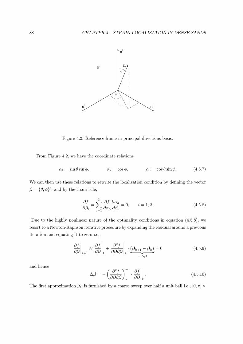
88 CHAPTER 4. STRAIN LOCALIZATION IN DENSE SANDS
q
f
n1
n2
n3
nR
3
Figure 4.2: Reference frame in principal directions basis.
From Figure 4.2, we have the coordinate relations
α1 = sin θ sinφ, α2 = cosφ, α3 = cos θ sinφ. (4.5.7)
We can then use these relations to rewrite the localization condition by defining the vector
β = θ, φt, and by the chain rule,
∂f
∂βi=
3∑
a=1
∂f
∂αa
∂αa∂βi
= 0, i = 1, 2. (4.5.8)
Due to the highly nonlinear nature of the optimality conditions in equation (4.5.8), we
resort to a Newton-Raphson iterative procedure by expanding the residual around a previous
iteration and equating it to zero i.e.,
∂f
∂β
∣∣∣∣k+1
≈ ∂f
∂β
∣∣∣∣k
+∂2f
∂β∂β
∣∣∣∣k
·(βk+1 − βk
)︸ ︷︷ ︸
:=∆β
= 0 (4.5.9)
and hence
∆β = −(
∂2f
∂β∂β
)−1
k
· ∂f∂β
∣∣∣∣k
. (4.5.10)
The first approximation β0 is furnished by a coarse sweep over half a unit ball i.e., [0, π]×

4.5. SEARCH ALGORITHM IN PRINCIPAL STRESS SPACE 89
[0, π], where the global minimum of the function f is attained.
Now, it remains to explicate the right hand side of equation (4.5.10). Using the fact
that ∂ det(A)/∂A = det(A)A−t
, along with the chain rule, we get
∂f
∂β= fA
−t:∂A
∂α· ∂α
∂β(4.5.11)
where ∂A/∂α is a third-order tensor with components (cf. equation (4.5.4))
∂Aab∂αc
=
2αaδaccepaa + 2αcτc + 2αcγca︸ ︷︷ ︸
c 6=a
if a = b
δac(cepab + γab
)αb + αa
(cepab + γab
)δbc if a 6= b
(no sum), (4.5.12)
with δab being the Kronecker delta. Further, the components of the matrix ∂α/∂β can be
easily computed to yield
∂α
∂β=
∂θα1 ∂φα1
∂θα2 ∂φα2
∂θα3 ∂φα3
. (4.5.13)
The Jacobian matrix can be calculated with the aid of the chain rule as
∂2f
∂β∂β=∂α
∂β· J · ∂α
∂β+∂f
∂α· ∂2α
∂β∂β, (4.5.14)
where
J = f
[(A
−t:∂A
∂α
)⊗(
A−t
:∂A
∂α
)− ∂A
∂α: A
−t ⊖ A−1
:∂A
∂α+ A
−t:∂2A
∂α∂α
].
(4.5.15)
Finally, the fourth order tensor ∂2A/(∂α∂α) can be written in component form as
1
2
∂Aab∂αc∂αd
=
δacδbdcepaa + δcdτc + δcdγca︸ ︷︷ ︸
c 6=a
if a = b
(cepab + γab
)Iabcd if a 6= b
(no sum), (4.5.16)
where Iabcd = 1/2 (δacδbd + δadδbc) is the fourth-order identity tensor.
Note that the tensors presented in equations (4.5.12,4.5.16) are very sparse, thus making
the assembly of the residual vector and the Jacobian matrix very straightforward. Also, the
Hessian matrix in (4.5.16) is only calculated once in the algorithm as it is not a function

90 CHAPTER 4. STRAIN LOCALIZATION IN DENSE SANDS
of the αa’s. At this point, it is easy to recognize the importance of the fact that since the
algorithm is based on Newton-Raphson scheme, asymptotic quadratic rate of convergence
is achieved and as a result the algorithm only needs to iterate a few times to find the global
minimum, provided, of course, that the first guess is close enough to the solution.
It has been shown by several researchers that for a wide class of elastoplastic models, at
least one of the αa’s is zero and therefore the search only needs to take place on the principal
planes [29, 35, 135, 136]. For example, classical models such as von-Misses, Drucker-Prager,
and Mohr-Coulomb can all be shown to localize within one of the principal planes, even for
the case of finite strains, provided a suitable form of the elastic continuum tangent is utilized
(isotropic). Also, the infinitesimal version of the elastoplastic model presented herein can
be shown to belong to the class of constitutive models described above. Due to the spectral
nature of the algorithm presented here, the on-plane feature is easily activated, thus making
the search very efficient. This feature is not present in some of the previously proposed
search algorithms available in the literature, see for example the works by Ortiz et al.
[51] and Mosler [137], which always perform fully three-dimensional searches. Simulations
underscoring the main features of the algorithm such as asymptotic quadratic rate and the
on-plane feature are included in the Numerical examples section.
Remark 5. Note that the formulation presented above is general and applicable to models
with linear and nonlinear kinematics. The same algorithm can be easily utilized for the
case of infinitesimal deformations provided that the stress terms are set identically equal to
zero, for example.
Remark 6. As pointed out first in [114], the consistent tangent operator can be used in lieu
of its continuum counterpart to search for the necessary condition for localization, provided
a small enough load step is taken. This can be accomplished, in light of the above described
search algorithm, by replacing cepab with cab and γab with γab. It is very convenient to use the
algorithmic operator as it is already available from the material subroutine and therefore
the continuum tangent is not to be used explicitly.
4.6 Numerical examples
In this section we conduct local stress-point simulations to illustrate the main features of the
three-invariant constitutive formulation developed in this work. Localization analyses are
conducted at this level and the convergence profile of the search algorithm for the minimum

4.6. NUMERICAL EXAMPLES 91
determinant is reported. Then, a series of boundary-value problems at the finite element
level are performed with the objective of studying the behavior of granular bodies exhibiting
unstructured random density fields. The simulations focus on detecting bifurcation and no
effort is made to try to capture post-bifurcation behavior. Hence all simulations are stopped
once bifurcation is detected.
4.6.1 Stress-point simulations
At the stress-point level, we performed two strain-driven simulations to highlight the dif-
ference in the responses resulting from the inclusion of the third stress invariant and to test
the performance of the search algorithm for the minimum value of the localization function.
Two material points with identical properties, except for the ellipticity parameters ρ and ρ,
were strained until they reached localization. The hyperelastic parameters are as follows:
compressibility coefficient κ = 0.01; reference elastic volumetric strain εev 0 = 0 at a refer-
ence pressure p0 = −100 kPa; initial shear modulus µ0 = 5400 kPa; and coupling constant
α0 = 0 (see section 4.2.1 for notation). The plasticity parameters are: plastic compress-
ibility coefficient λ = 0.0135; critical state parameter M = 1.2; shape parameters N = 0.4
and N = 0.2 (nonassociative volumetric plastic flow); and hardening constant h = 280 (see
section 4.2.2 for notation). Both material points were initially denser than critical with
an initial specific volume v = 1.59 and a reference specific volume vc0 ≈ 1.81. The only
difference in material properties is the ellipticity: one material point had ρ = ρ = 1 (two-
invariant formulation, circular cross-section and associative flow on the deviatoric plane)
and the other had ρ = 0.7 and ρ = 0.8 (non-circular, convex cross-section, nonassociative
flow on deviatoric plane). Both material points were modeled using the Willam-Warnke
shape function in equation (4.2.12).
The loading protocol is as follows. We prescribed two equal sets of relative deformation
gradient fn+1 = ∂xn+1/∂xn: the first set was prescribed over n1 steps, followed by the
second for n2 steps until localization was reached. The two relative deformation gradients
are
f1 =
1 + λ2 0 0
0 1 − λ1 0
0 0 1
and f2 =
1 0 0
0 1 − λ2 0
0 0 1 + λ1
, (4.6.1)

92 CHAPTER 4. STRAIN LOCALIZATION IN DENSE SANDS
-600 -500 -400 -300 -200 -100 0-150
-100
-50
0
50
100
150
TAU3", kPa
TA
U2",
kP
aRHO = 1.0
RHO = 0.7
OABC
A’
B’
C’
Figure 4.3: Stress paths on meridian plane. Yield surfaces expand from A to B and to Cwhereas stress paths follow O–A′–B′–C ′ trajectory.
hence, the total deformation gradient is
F = fn2
2 · fn1
1 , (4.6.2)
where λ1 = 1×10⁻³ and λ2 = 4×10⁻⁴. The material points were mostly compressed in the
first n1 = 10 steps, and then mostly stretched in the subsequent n2 steps, hence the total
number of steps is given by n = n1 + n2. The stress paths followed by the two material
points are shown in Figures 4.3 and 4.4, with Figure 4.3 showing the stress paths on a
meridian plane and Figure 4.4 showing them on a deviatoric plane. The paths are plotted
using rotated principal stress axis as described in [111]. The trajectories followed by the
two stress points are similar. The stress paths started at point O and then were loaded
to point A′ after the first n1 steps, and subsequently deformed to points B′ and C ′, where
they localized. Similarly, the yield surfaces expanded from A to B to C, without softening.
The sample with ρ = 0.7 localized first at n = 22, whereas the sample with ρ = 1
localized at n = 26. The function F (A) for both stress points is plotted in Figure 4.5
where we see minor differences in the trajectories, yet the stress point with ρ = 0.7 localized
sooner. Hence, the third invariant enhances strain localization. The values for the function

4.6. NUMERICAL EXAMPLES 93
-150 -100 -50 0 50 100 150-150
-100
-50
0
50
100
150
TAU1", kPa
TA
U2
, kP
a"
RHO = 1.0
RHO = 0.7
O
A
B
C
A’
B’
C’
Figure 4.4: Stress paths on deviatoric plane. Yield surfaces expand from A to B and to Cwhereas stress paths follow O–A′–B′–C ′ trajectory.
F (A) are obtained by the search algorithm outlined in Section 4.5 by sweeping the R3
space via the angles θ and φ. One such a profile swept by the search algorithm is shown
in Figure 4.6, where the determinant of the acoustic tensor is plotted as a function of θ
and φ at the onset of localization for the material point with ρ = 0.7. One such profile is
swept at each time step where the search algorithm finds one of usually two wells and then
returns a solution. One interesting note from Figure 4.6 is that localization was achieved
at φ = π/2 (see end of section 4.5 for discussion). Finally, the convergence profile for the
search algorithm at various load steps is reported in Figure 4.7 where optimal quadratic
convergence is observed.
4.6.2 Simulations with cubical specimens
Randomization of the density field in a specimen is achieved through the void ratio e,
defined as the ratio between the volume occupied by empty voids and the intrinsic volume
of the solid phase, i.e., e := Vv/Vs. The main issue concerns finding a plausible probability
density function describing the natural dispersion of voids in a sample of granular materials.
Shahinpoor [138] used statistical mechanical theory on a collection of Voronoi cells to obtain
an exact expression for the probability density function for the distributions of void ratio

94 CHAPTER 4. STRAIN LOCALIZATION IN DENSE SANDS
10 12 14 16 18 20 22 24 26−0.2
0
0.2
0.4
0.6
0.8
1
STEP NO.
NO
RM
ALI
ZE
D M
INIM
UM
DE
TE
RM
INA
NT
RHO = 1.0RHO = 0.7
Figure 4.5: Minimum determinant of the acoustic tensor at various load steps.
0 50 100 1500
20
40
60
80
100
120
140
160
180
THETA, deg
PH
I, de
g
0
0.5
1
1.5
2
2.5
3
3.5
x 1011
ALGO SOLN
Figure 4.6: Profile of the determinant of the acoustic tensor for three-invariant model withρ = 0.7 at onset of localization.

4.6. NUMERICAL EXAMPLES 95
1 2 3 4 510
−15
10−10
10−5
100
ITERATION
NO
RM
ALI
ZE
D R
ES
IDU
AL
STEP NO. 5STEP NO. 10STEP NO. 15STEP NO. 20TOLERANCE
Figure 4.7: Convergence profile for search algorithm at various load steps.
in a random aggregate of granular material. The probability distribution function for e was
established to be a truncated exponential distribution. It also has been used by Nubel and
Huang [19] to study localized deformation patterns in granular media.
Here, we adopted a truncated exponential density function for e of the form
fe(e) =γ exp (−γe)
exp (−γed) − exp (−γel), (4.6.3)
where ed is the lower bound of the distribution corresponding to the densest state, el is the
upper bound of the distribution corresponding to the loosest state, and γ plays the role of a
fitting parameter. We used these bounds to restrict the amount of dispersion in the density
of the sample, thus controlling the amount of inhomogeneities. The expected value of the
distribution is given by [139]
e =
∫ el
ed
efe (e) de, (4.6.4)
where
e =1
γ+ed exp(−γed) − el exp(−γel)
exp(−γed) − exp(−γel), (4.6.5)
Hence, we can prescribe the expected value or mean void ratio e subject to the upper and
lower bounds ed and el, respectively, provided we solve for the fitting coefficient γ. This is

96 CHAPTER 4. STRAIN LOCALIZATION IN DENSE SANDS
easily accomplished by a Newton-Raphson scheme on the residual
r (γ) = e− 1
γ− ed exp(−γed) − el exp(−γel)
exp(−γed) − exp(−γel). (4.6.6)
The random density field was then generated on the assumption that the values of void
ratio in space are mutually independent. For this reason, these random fields are called
“unstructured” due to the lack of correlation in the density field between points A and B
in the same sample.
We then sheared in compression two rectangular specimens with dimensions 1×1×2 m
and assumed to behave according to the constitutive framework presented above, up to the
onset of localization. The material properties for both specimens were identical to those of
the stress-point with ρ = ρ = 0.78 and vc0 ≈ 1.85 discussed in the previous section. The
Argyris-Gudehus shape function given in equation (4.2.11) was utilized in the simulations.
At the structural level the density field was generated using the exponential distribution
described above with a mean void ratio e = 0.63 and lower and upper bounds ed = 0.54
and el = 0.64, respectively. Hence, the two specimens, which we will call ‘INHOMOGE-
NEOUS 1’ and ‘INHOMOGENEOUS 2’ for identification purposes, represent two different
realizations of the same distribution function for the void ratio field, with otherwise identi-
cal mechanical properties. Figure 4.8 shows the discretized specimens with their respective
initial specific volume field v := 1+e. The rectangular domains were discretized using 2000
trilinear hexahedral elements equipped with the B-bar method for nonlinear kinematics
using the so-called mean dilation technique [120, 121] (see [119] for a survey on the B-bar
method).
The boundary conditions applied to the specimens were as follows. All four lateral faces
were initially subjected to a constant confining pressure of 100 kPa (Newman BCs). The
bottom and top faces of the specimens (z = 0, 1 m) were supported by rollers with a pin
at the (0, 0, 0)m point for stability (Dirichlet BCs). The bottom face was constrained from
displacement in the z-direction, whereas the top face was subjected to a vertical displace-
ment responsible for shearing the samples in compression. The samples were loaded in two
phases. Phase one, an all-around confining pressure was applied to consolidate the sample
followed by phase two, where the top face was displaced vertically. The objective of this
loading protocol, favoring homogeneous deformations in perfectly homogeneous samples, is
twofold: to observe if any significant differences are introduced by perturbing the density

4.6. NUMERICAL EXAMPLES 97
0
0.5
1
0
0.5
10
0.5
1
1.5
2
x−axisy−axis
z−axis
0
0.5
1
0
0.5
10
0.5
1
1.5
2
x−axisy−axis
z−axis
1.59
1.595
1.6
1.605
1.61
1.615
1.62
1.625
1.63
1.635
1.64
INHOMOGENEOUS 1 INHOMOGENEOUS 2
Figure 4.8: Initial specific volume field and finite element discretization for inhomogeneousrectangular specimens.
field by comparing the homogeneous response against perturbed responses from the samples
shown in Figure 4.8, and to compare the responses of two inhomogeneous samples from two
realizations of the density field. To this end, a homogeneous sample with constant void
ratio v = 1.63 was subjected to the same BCs described above, and its response compared
against its inhomogeneous counterparts.
Figure 4.9 shows the contours of the function F (A), for both inhomogeneous samples,
superimposed on the deformed mesh at the onset of localization. Here, we define localization
when one or more Gauss points have detected the first negative incursion of the function
F (A) (even though contours appear as positive due to averaging necessary for plotting).
Both inhomogeneous samples localized at a nominal axial strain of around 5.8%, yet, from
Figure 4.9, we observe that the deformation patterns and the inclinations of the impending
shear bands are conjugate to each other, almost looking as mirror images. This same trend is
observed in Figure 4.10 which compares the contours of the total deviatoric strain invariant
on both inhomogeneous samples. Comparing Figures 4.9 and 4.10, note a strong correlation
between the vanishing of the determinant of the acoustic tensor and the localized values of
the deviatoric component of deformation (shear strains).
Figure 4.11 shows the nominal axial stress as a function of the nominal axial strain for

98 CHAPTER 4. STRAIN LOCALIZATION IN DENSE SANDS
0
0.5
1
0
0.5
1
0
0.5
1
1.5
x−axisy−axis
z−axis
0
0.5
1
0
0.5
1
0
0.5
1
1.5
x−axisy−axis
z−axis
0.5
1
1.5
2
2.5
x 1011INHOMOGENEOUS 1 INHOMOGENEOUS 2
Figure 4.9: Contour of function F (A) at onset of localization for inhomogeneous rectangularspecimens.
0
0.5
1
0
0.5
1
0
0.5
1
1.5
x−axisy−axis
z−axis
0
0.5
1
0
0.5
1
0
0.5
1
1.5
x−axisy−axis
z−axis
0.03
0.04
0.05
0.06
0.07
0.08
0.09
0.1
0.11
INHOMOGENEOUS 1 INHOMOGENEOUS 2
Figure 4.10: Deviatoric strain invariant field at onset of localization for inhomogeneousrectangular specimens.

4.6. NUMERICAL EXAMPLES 99
0 5 10 15 20100
150
200
250
300
350
400
450
500
NOMINAL AXIAL STRAIN, %
NO
MIN
AL
AX
IAL
ST
RE
SS
, kP
a
HOMOGENEOUSINHOMOGENEOUS 1INHOMOGENEOUS 2
LOCALIZATION
Figure 4.11: Nominal axial stress response for rectangular specimens.
both inhomogeneous specimens and their homogeneous counterpart. We see a close agree-
ment in the global responses up to about 4% nominal axial strain, where the inhomogeneous
responses softened and eventually localized at 5.8% strain. The homogeneous sample, how-
ever, underwent very little softening and in fact continued to harden. The change in volume
experienced by the heterogeneous and homogeneous samples are compared in Figure 4.12.
Unlike Figure 4.11, the responses seem identical throughout the duration of the simulations.
Note that the samples compacted first, and then dilated. This trend is very common in
dense sands.
From these simulations we conclude that perturbations in the density field via inhomo-
geneities at the meso-scale tend to trigger the onset of localization. Also, as we compare
the responses of two nearly identical inhomogeneous samples, we observe localization pat-
terns that are conjugate of each another. The mechanical responses of the heterogeneous
samples in the early stages of deformation are very similar to those of their homogeneous
counterpart, suggesting that we can calibrate the meso-scale model parameters from global
specimen responses during the early stages of loading.

100 CHAPTER 4. STRAIN LOCALIZATION IN DENSE SANDS
0 5 10 15 20−0.02
0
0.02
0.04
0.06
0.08
0.1
0.12
0.14
NOMINAL AXIAL STRAIN, %
∆ V
OLU
ME
, m3
HOMOGENEOUSINHOMOGENEOUS 1INHOMOGENEOUS 2
LOCALIZATION
Figure 4.12: Volume change response for rectangular specimens.
4.6.3 Simulations with cylindrical specimens
Next, two inhomogeneous cylindrical specimens exhibiting random unstructured density
fields were loaded in biaxial compression with BCs (and geometry) that emulated ‘triaxial’
testing in the laboratory. Both specimens are 2 m in diameter and 4 m tall. The elastoplastic
properties of these specimens are identical to those in the simulations with cubical specimens
described above. However, here we used two different density fields to simulate the effects
of increasing the spread in the random field on the localization properties of dense sand
samples. To this end, the first inhomogeneous sample, which we call ‘INHOMO 1.58-1.61’,
has a density field such that e = 0.59, with lower and upper bounds ed = 0.58 and el = 0.61,
representing a relatively narrow distribution of void ratio. As for the second sample, we
increased the spread in the void ratio field while keeping the mean constant, i.e., e = 0.59,
with lower and upper bounds ed = 0.56 and el = 0.68. We will call this specimen ‘INHOMO
1.56-1.68’. Figure 4.13 displays the initial specific volume field superimposed on the original
configuration for both inhomogeneous samples. The cylindrical domains were discretized
using 1280 eight-node brick elements equipped with the B-bar method.
As for the BCs, the specimens were biaxially loaded with a confining pressure applied on
the sleeve of the cylinders (Neumann BC) while the top and bottom faces were supported

4.6. NUMERICAL EXAMPLES 101
−1
0
1
−1
0
10
1
2
3
4
x−axisy−axis
z−axis
1.582
1.584
1.586
1.588
1.59
1.592
1.594
1.596
1.598
1.6
−1
0
1
−1
0
10
1
2
3
4
x−axisy−axis
z−axis
1.57
1.58
1.59
1.6
1.61
1.62
1.63
INHOMO 1.58-1.61 INHOMO 1.56-1.68
Figure 4.13: Initial specific volume field and finite element discretization for inhomogeneouscylindrical specimens.
on rollers (Dirichlet BC). The point (0, 0, 0)m in the specimens was supported by a pin for
stability. As in the rectangular specimen simulations, the bottom face was constrained to
move vertically while the top face was compressed to mimic a homogeneous deformation.
The samples were then loaded as before, with an initial confining pressure of 100 kPa
followed by axial compression from the top face until localization was detected.
Figures 4.14 and 4.15 show an ‘X-ray’ rendering of the deviatoric strain invariant and the
function F (A), respectively, superimposed on different cut-planes in the deformed configu-
ration for the ‘INHOMO 1.58-1.61’ sample. The sub-figures on the right show longitudinal
panels while the sub-figures on the left show axial planes. Note a localized area of intense
shearing going from the top-right to the bottom-left corner, compared with the rest of the
sample that experienced lower values of shear strains. Similar trends were observed on the
‘INHOMO 1.56-1.68’ sample.
Figures 4.16 and 4.17 show nearly identical plots of the overall axial stress-axial strain
and volumetric strain-axial strain for both inhomogeneous samples and their homogeneous
counterpart with e = 1.59. The inhomogeneous samples localized at different instants
whereas the homogeneous sample did not localize at all. Sample ‘INHOMO 1.56-1.68’
localized at 4.38% whereas ‘INHOMO 1.58-1.61’ localized at 4.76%. The global convergence

102 CHAPTER 4. STRAIN LOCALIZATION IN DENSE SANDS
−1
0
1
−1
0
1
0
0.5
1
1.5
2
2.5
3
3.5
x−axisy−axis
z−axis
−1
0
1
−1
0
1
0
0.5
1
1.5
2
2.5
3
3.5
x−axisy−axis
z−axis
0.03
0.035
0.04
0.045
0.05
0.055
0.06
0.065
0.07
0.075
0.08
Figure 4.14: Total deviatoric strain invariant on various cut-planes at the onset of localiza-tion for sample ‘INHOMO 1.58-1.61’.
−1
0
1
−1
0
1
0
0.5
1
1.5
2
2.5
3
3.5
x−axisy−axis
z−axis
−1
0
1
−1
0
1
0
0.5
1
1.5
2
2.5
3
3.5
x−axisy−axis
z−axis
1.2
1.4
1.6
1.8
2
2.2
2.4
2.6
2.8
3
x 1011
Figure 4.15: Determinant of acoustic tensor on various cut-planes at the onset of localizationfor sample ‘INHOMO 1.58-1.61’.

4.7. CLOSURE 103
0 1 2 3 4 5100
150
200
250
300
350
400
450
500
NOMINAL AXIAL STRAIN, %
NO
MIN
AL
AX
IAL
ST
RE
SS
, kP
a HOMOGENEOUSINHOMO 1.58−1.61INHOMO 1.56−1.68
LOCALIZATION
Figure 4.16: Nominal axial stress response for cylindrical specimens.
profile for the sample ‘INHOMO 1.56-1.68’ is reported in Figure 4.18, showing optimal rate
of convergence.
4.7 Closure
We have presented a critical state plasticity model that utilizes all three invariants of the
stress tensor for deformation and strain localization analyses of granular materials with
random unstructured density at the meso-scale. For the implementation we have used
the classical return mapping algorithm in the direction of the elastic logarithmic principal
stretches. An iterative algorithm based on Newton’s method was shown to deliver optimal
performance. We also have presented a search algorithm for the minimum determinant of the
acoustic tensor on the elastic principal stretch planes. Boundary-value problems mimicking
soil samples have been analyzed using a truncated exponential distribution to generate
random and unstructured density fields. Results of numerical simulations suggest that
inhomogeneities tend to trigger strain localization, with heterogeneous samples localizing
when their equivalent homogeneous counterparts would not. Results of the studies also
suggest that heterogeneity in the density field tends to enhance and accelerate the onset of
strain localization, even if the initial global deformation responses of a homogeneous sample

104 CHAPTER 4. STRAIN LOCALIZATION IN DENSE SANDS
0 1 2 3 4 5−0.1
−0.08
−0.06
−0.04
−0.02
0
0.02
NOMINAL AXIAL STRAIN, %
∆ V
OLU
ME
, m3 HOMOGENEOUS
INHOMO 1.58−1.61INHOMO 1.56−1.68
LOCALIZATION
Figure 4.17: Volume change response for cylindrical specimens.
1 2 3 4 5 6 7 810
−15
10−10
10−5
100
ITERATION
NO
RM
ALI
ZE
D R
ES
IDU
AL
STEP NO. 45STEP NO. 90STEP NO. 135STEP NO. 180TOLERANCE
Figure 4.18: Convergence profile for finite element solution at various load steps.

4.7. CLOSURE 105
and its heterogeneous counterpart appear to be the same. The framework presented in this
paper is useful for investigating strain localization phenomena in heterogeneous granular
materials at a finer scale.
Acknowledgments
This work has been supported by National Science Foundation under Grant Nos. CMS-
0201317 and CMS-0324674 to Stanford University. The first author is grateful to Professor
Adrian Lew of Stanford University for enlightening discussions regarding constitutive theory
and Lie derivatives. We also thank the two anonymous reviewers for their constructive
reviews.

106 CHAPTER 4. STRAIN LOCALIZATION IN DENSE SANDS

Chapter 5
Modeling deformation banding in
dense and loose fluid-saturated
sands
This Chapter will be published in: J. E. Andrade and R. I. Borja. Modeling deformation
banding in dense and loose fluid-saturated sands. Finite Elements in Analysis and Design,
2006. In review for the 18th Annual Melosh Competition Special Issue.
Abstract
Balance of mass and linear momentum of a solid-fluid mixture furnish a complete set of
equations from which the displacements of the solid matrix and the pore pressures can be
resolved for the case of quasi-static loading, resulting in the so-called u − p Galerkin for-
mulation. In this work, a recently proposed model for dense sands is utilized to model the
effective stress response of the solid matrix appearing in the balance of linear momentum
equation. In contrast with other more traditional models, inherent inhomogeneities in the
porosity field at the meso-scale are thoroughly incorporated and coupled with the macro-
scopic laws of mixture theory. Also, the hydraulic conductivity is naturally treated as a
function of the porosity in the solid matrix, allowing for a more realistic representation of
the physical phenomenon. The aforementioned balance laws are cast into a fully nonlin-
ear finite element program utilizing isoparametric elements satisfying the Babuska-Brezzi
107

108 CHAPTER 5. MODELING DEFORMATION BANDING IN SATURATED SANDS
stability condition. Criteria for the onset of localization under locally drained and locally
undrained conditions are derived and utilized to detect instabilities. Numerical simulations
on dense and loose sand specimens are performed to study the effects of inhomogeneities
on the stability of saturated porous media at the structural level.
5.1 Introduction
Deformation banding is one of the most common failure modes in geomaterials such as rock,
concrete, and soil. It is well known that appearance of bands of intense localized deformation
significantly reduces the load-carrying capacity of any structure that develops them [20,
140]. Furthermore, when dealing with fluid-saturated geomaterials, the interplay between
the contraction/dilation of pores and development of pore fluid pressures is expected to
influence not only the strength of the solid matrix but also its ability to block or transport
such fluids [12]. Accurate and thorough simulation of these phenomena (i.e., deformation
banding and fluid flow) requires numerical models capable of capturing fine-scale mechanical
processes such as mineral particle rolling and sliding in granular soils and the coupling
between porosity and relative permeability. Until recently, these processes could not even
be observed in the laboratory. Numerical models could only interpret material behavior as
a macroscopic process and were, therefore, unable to model the very complex behavior of
saturated geomaterials accurately.
In this paper, we study the deformation-diffusion behavior of a two-phase system of
soil and fluid. It is well known that the coupling between the mechanical behavior of the
underlying drained solid and the fluid flow can lead to sharply distinct behavior of the over-
all mixed system. For instance, dilative saturated rock masses can lead to a phenomenon
called ‘dilatant hardening’, which, as the name implies, tends to delay the onset of strain
localization because effective pressures tend to increase and hence strengthen the sample
in general [44, 141, 142]. On the other hand, relatively loose sands tend to compact when
sheared. Therefore, when pores compact faster than the rate at which fluids can escape,
pore fluid pressure increases and the effective pressure decreases, leading to a phenomenon
known in the geotechnical community as ‘liquefaction’ [3, 13, 14]. Consequently, it is im-
portant to study the deformation-diffusion behavior in saturated granular media taking into
account the effect of pore contraction/dilation and its influence on the relative density and
permeability of the solid matrix. This is accomplished in this study.

5.1. INTRODUCTION 109
Even though the interplay between fluid flow and solid deformation using finite elements
has been studied before, the focus of models dealing with fully saturated and partially
saturated soils has been on ‘homogeneous’ material response [45, 55, 143–150]. This has
been a natural approach given the fact that the technology to infer material inhomogeneities
in the laboratory has only been recently developed. Therefore, numerical models dealing
with the simulation of strain localization have either imposed inhomogeneous deformation
fields (e.g., [55, 143, 144]) or introduced arbitrary weaknesses in the otherwise pristine
specimens (e.g., [50–52, 62]).
New advances in laboratory experimentation, such as X-Ray Computed Tomography
(CT) and Digital Image Correlation (DIC) techniques, allow accurate observation of key
parameters associated with material strength and provide the motivation for the develop-
ment of more realistic models that incorporate information at a scale finer than specimen
scale (see works in [4, 15, 16] for applications of X-Ray CT and [83, 151] for applications of
DIC). In this paper, we adopt a refined constitutive model based on a meso-scale descrip-
tion of the porosity to simulate the development (location and direction) of deformation
bands on saturated samples of sand. The effective stress behavior of the granular material
is assumed to be governed by an elastoplastic model for sands developed by the authors
in [122, 152]. The ability of the model to incorporate data depicting the inherent inho-
mogeneities in samples of sand at the meso-scale provides a natural and realistic source
of inhomogeneity that, as we shall demonstrate subsequently, affects the stability and flow
characteristics of sand specimens. As a matter of terminology the ‘meso-scale’ here refers
to a scale smaller than specimen size but larger than particle size. In a typical sample
encountered in the laboratory, the meso-scale refers to the millimeter scale.
The constitutive model for the effective stresses is a member of the critical state plasticity
family of models. It is based on an original model proposed by Jefferies in [2] and extended
by the authors in [122, 152]. Two main features distinguish this model from its critical
state predecessors. First, the yield surface is allowed to ‘detach’ from the critical state
line by introducing a state parameter ψ [106], allowing a state point to lie either above or
below the critical state line (CSL). Through the state parameter ψ we are able to prescribe
spatial values of porosity across the sample, which constitutes the connection to the meso-
scale. Second, the model features a nonassociative flow rule and a three stress-invariant
formulation, for capturing important features of sand behavior [153].
The model for the two-phase system is based on the theory of mixtures [154, 155], which

110 CHAPTER 5. MODELING DEFORMATION BANDING IN SATURATED SANDS
serves as the underlying theoretical block to develop balance laws for multi-phase bodies.
Saturated granular media is modeled as a two-phase system composed of a solid phase and a
fluid phase. This study extends the work of Li et al. [156] who considered elastic expulsion
of fluids at finite strain and also extends the work by Armero [143] who looked at the
strain localization behavior of homogeneous saturated samples of soil—obeying a generalized
Drucker-Prager constitutive model—under boundary conditions favoring inhomogeneous
deformations. Furthermore, here the fluid content is not decomposed into elastic and plastic
parts as the porosity field is naturally coupled to the elastoplastic formulation emanating
from the constitutive law for the porous matrix. The numerical implementation also differs
from that of Armero [143] as it does not rely on the operator split technique, but rather
solves the coupled system of nonlinear equations directly. It is worthwhile noting that
Armero and Callari [157] and Callari and Armero [47] expanded the work by Armero [143]
by developing a strong discontinuity model to model deformation banding in homogeneous
saturated media at finite strains.
In this work, fluid-saturated porous media is modeled using nonlinear continuum me-
chanics and a novel constitutive model for sands. Furthermore, the effect of porosity is also
accounted for by utilizing the Kozeny-Carman equation which relates the intrinsic perme-
ability to the porosity [158]. The objective of this paper is to study the effect of fluctuations
in porosity at the meso-scale on the stability and transport properties of samples of dense
and loose sand analyzed as boundary-value problems.
Using the balance laws for the system, along with the concept of effective stresses, the
strong form of the deformation-diffusion problem at finite deformations is developed. The
variational form is obtained as a two-field mixed formulation where the displacements in
the solid matrix u and the Cauchy fluid pressures p serve as basic unknowns. Thus, a
classical u−p formulation is obtained and discretized in space using elements satisfying the
Babuska-Brezzi stability condition [119, 159]. The linearization of the variational equations
serve as the building block to develop expressions for the acoustic tensor for two extreme
cases: the case of locally drained behavior and the case of locally undrained behavior. These
expressions for the acoustic tensor are then utilized in the analysis of localization of strain
for a fully saturated medium.
The structure of the paper is as follows. In Section 5.2 the conservation of mass and
linear momentum equations for a two-phase mixture are derived. Section 5.3 describes

5.2. BALANCE LAWS: CONSERVATION OF MASS AND LINEAR MOMENTUM 111
the constitutive framework utilized in the formulation. In particular, the concept of effec-
tive stress is introduced and the model governing the effective stresses is briefly described.
Darcy’s law is presented as the fundamental constitutive equation for fluid flow. In Section
5.4, the finite element solution procedure is presented and the linearization of the variational
equations is addressed in detail. Section 5.5 addresses the extreme criteria for localization
in fluid-saturated media. The framework described above is then utilized in a series of
numerical examples presented in Section 5.6, where it is shown that the stability and flow
properties of samples of sand is profoundly influenced by meso-scale inhomogeneities in the
initial porosity field.
As for notations and symbols used in this paper, bold-faced letters denote tensors and
vectors; the symbol ‘·’ denotes an inner product of two vectors (e.g. a ·b = aibi), or a single
contraction of adjacent indices of two tensors (e.g. c · d = cijdjk); the symbol ‘:’ denotes
an inner product of two second-order tensors (e.g. c : d = cijdij), or a double contraction
of adjacent indices of tensors of rank two and higher (e.g. C : ǫe = Cijklǫekl); the symbol
‘⊗’ denotes a juxtaposition, e.g., (a ⊗ b)ij = aibj . Finally, for any symmetric second order
tensors α and β, (α ⊗ β)ijkl = αijβkl, (α ⊕ β)ijkl = βikαjl, and (α ⊖ β)ijkl = αilβjk.
5.2 Balance laws: conservation of mass and linear momen-
tum
Consider a two-phase mixture of solids and fluid. The balance equations are obtained by
invoking the classical mixture theory (see for example the works in [154, 155]). Within this
context, each α-phase (α = s, f, for solid and fluid, respectively) or constituent occupies
a volume fraction, φα := Vα/V , where Vα is the volume occupied by the α-phase and
V = Vs + Vf is the total volume of the mixture. Naturally,
φs + φf = 1. (5.2.1)
The total mass of the mixture is defined by the mass contribution from each phase i.e.,
M = Ms+Mf . The inherent or true mass density for the α-phase is defined as ρα := Mα/Vα.
Also, the apparent or partial mass density is given by ρα = φαρα. Therefore, the total mass
density is given by
ρ = ρs + ρf . (5.2.2)

112 CHAPTER 5. MODELING DEFORMATION BANDING IN SATURATED SANDS
Furthermore, both phases are assumed to be superimposed on top of each other and hence,
a point x in the mixture is occupied by both solid and fluid simultaneously.
From this point forward, all inherent or true quantities pertaining to the α-phase are
designated with a subscript, whereas apparent or partial quantities are designated with a
superscript as a general notation.
5.2.1 Balance of mass
In deriving the balance laws, it is relevant to pose all time derivatives following a particular
phase. From Figure 5.1, we note that the current configuration of the mixture in a region
Ω is defined by the mapping of the solid-phase ϕs (Xs, t), where Xs ≡ X is the position
vector in the reference configuration Ωs0 ≡ Ω0, and the mapping of the fluid-phase ϕf (X f , t),
where X f is the position vector in the reference configuration Ωf0. Hence, it is convenient
to define the total time-derivative following the α-phase such that
dα ()
dt=∂ ()
∂t+ ∇x () · vα, (5.2.3)
where ∇x () ≡ ∂/∂x is the gradient operator with respect to the current configuration Ω
and vα ≡ ∂ϕα/∂t is the velocity vector of the α-phase. For simplicity of notation and where
there is no room for ambiguity, we drop the subscripts and superscripts for all quantities
pertaining to the solid-phase, as we will write all balance laws following this phase. It is
thus straight-forward to check the identity
df ()
dt=
d ()
dt+ ∇x () · v, (5.2.4)
where v := vf − v is the relative velocity vector and d/dt () ≡ ˙() is the total material
time derivative following the solid-phase.
Consider the expression for the total mass of α-phase in the current configuration i.e.,
mα ≡∫
Ωφαρα dΩ =
∫
Ωα0
φαραJα dΩα0 , α = s, f, (5.2.5)
which has been pulled back to the reference configuration of the α-phase via the mapping
ϕ−1α and where Jα = detF α is the Jacobian of the deformation gradient tensor F α ≡
∂ϕα/∂Xα. If there is no production of α-phase mass and there are no mass exchanges

5.2. BALANCE LAWS: CONSERVATION OF MASS AND LINEAR MOMENTUM 113
js
W0
W
x1
x2
X
x
jf
W0
f
Figure 5.1: Current configuration Ω mapped from respective solid and fluid reference con-figurations.
amongst phases, conservation of mass implies
dα
dtmα =
∫
Ωα0
dα
dt(φαραJα) dΩα
0 = 0, α = s, f, (5.2.6)
which after classical continuity arguments yields the localized form of the conservation of
mass for the α-phasedα
dtρα + ρα∇x·vα = 0, (5.2.7)
where ∇x· () is the divergence operator with respect to the current configuration. Making
use of equation (5.2.7) and identity (5.2.4) the conservation of mass equation for the solid
and fluid phases are, respectively,
ρs + ρs ∇x·v = 0 (5.2.8a)
ρf + ρf ∇x·v = −∇x· q, (5.2.8b)
where q ≡ ρf v is the Eulerian relative flow vector of the fluid phase with respect to the
solid matrix. Adding equations (5.2.8a) and (5.2.8b), we get the basic conservation of mass
114 CHAPTER 5. MODELING DEFORMATION BANDING IN SATURATED SANDS
equation for the system, i.e.,
ρ0 = −J ∇x· q, (5.2.9)
where ρ0 ≡ Jρ is the pull-back mass density of the mixture in the reference configuration.
It is clear from the above equation that in the case of locally undrained deformations (i.e.,
when both phases of the mixture move as one) q ≈ 0 and thus the relative mass flux term
in the right-hand side drops out and the classical conservation of mass for a mono-phase
body is captured.
Equations (5.2.8a) and (5.2.8b) are typically simplified by recalling the definition of
the partial densities and introducing the bulk modulus. For barotropic flows, there exists a
functional relationship of the form fα (pα, ρα) = 0, where pα is the intrinsic Cauchy pressure
in the α-phase or the force acting on this phase per unit area of the same phase [116, 156].
Thus, it is meaningful to define the bulk modulus of the alpha phase such that
Kα = ραdpαdρα
, α = s, f, (5.2.10)
and therefore equations (5.2.8a) and (5.2.8b) can then be rewritten, respectively, as
φs + φs
(ps
Ks+ ∇x·v
)= 0 (5.2.11a)
φf + φf
(pf
Kf+ ∇x·v
)= − 1
ρf∇x· q. (5.2.11b)
Adding the last two equations and recalling equation (5.2.1), we get
φs ps
Ks+ φf pf
Kf+ ∇x·v = − 1
ρf∇x· q. (5.2.12)
The above equation can be expressed in terms of the Kirchhoff intrinsic pressures by
recalling the relationship between the Kirchhoff and Cauchy stress tensors, i.e., τα ≡ Jσα
and as a result the Kirchhoff pressure for the α-phase is defined as ϑα = Jpα. Using the
identity J = J ∇x·v [30] we express equation (5.2.12) as
φs ϑs
Ks+ φf ϑf
Kf+ J
[1 − φs
J
ϑs
Ks− φf
J
ϑf
Kf
]= − J
ρf∇x· q. (5.2.13)

5.2. BALANCE LAWS: CONSERVATION OF MASS AND LINEAR MOMENTUM 115
Equation (5.2.13) is complete in the sense that neither constitutive nor kinematic assump-
tions have been introduced. In geomechanical applications, a typical and plausible assump-
tion is to treat the solid phase as incompressible, and consequently Ks → ∞. Then, the
reduced balance of mass equation for the mixture can be written as
φf ϑf
Kf+ J
[1 − φf
J
ϑf
Kf
]= − J
ρf∇x· q. (5.2.14)
Finally, we can write the Lagrangian balance of mass equation by making use of the Piola
identity, i.e. ∇X·(JF−t
)= 0 where ∇X· () is the divergence operator with respect to the
reference configuration of the solid phase and the superscript ‘t’ is the transpose operator.
Thus,
J ∇x· q = ∇X·Q, (5.2.15)
where Q ≡ JF−1 · q is the Piola transform of the Eulerian vector q. Therefore, the
Lagrangian balance of mass equation takes the form, cf. equation (5.2.9),
ρ0 = −∇X·Q. (5.2.16)
5.2.2 Balance of linear momentum
At this point, it is necessary to introduce the concept of partial stresses in a more rigorous
way. Let σα denote the Cauchy partial stress tensor for the α-phase. The total Cauchy
stress tensor is obtained from the sum [46, 155, 160]
σ = σs + σf . (5.2.17)
From the above definition, an expression for the partial Cauchy pressure or mean normal
stress for the α-phase can be readily obtained, i.e. pα ≡ −1/3 trσα and hence, the intrinsic
Cauchy pressures can be defined such that
ps = − 1
3φstrσs and pf = − 1
3φftrσf . (5.2.18)
Also, the associated first Piola-Kirchhoff partial stress tensor can be defined as P α =
Jσα · F−t, the total first Piola-Kirchhoff stress tensor is given by
P = P s + P f . (5.2.19)

116 CHAPTER 5. MODELING DEFORMATION BANDING IN SATURATED SANDS
The linear momentum acting on the α-phase is given by [154, 155, 161]
lα =
∫
Ωραvα dΩ, (5.2.20)
whereas the resulting forces acting on the phase are [46]
rα =
∫
Ω(φαραg + φαhα) dΩ +
∫
Γφαtα dΓ, (5.2.21)
where g is the gravity vector. The first term in (5.2.21) results from the body forces acting
on the α-phase, the second term comes from the forces exerted on the α-phase from other
phases in the mixture, and the third term emanates from the tractions imposed on the
phase at the boundary Γ. Note that the partial traction is related to the partial Cauchy
stress on the α-phase via the tetrahedron theorem i.e., tα ≡ φαtα = σα · n, where n is a
unit vector normal to the surface Γ.
Balance of linear momentum on the α-phase necessitates
dα
dtlα = rα, (5.2.22)
and after pull-back and push-forward operations and enforcing balance of mass, see equation
(5.2.7), we get ∫
Ωραaα dΩ = rα, (5.2.23)
where aα ≡ dαvα/dt is the absolute acceleration vector for the α-phase. Once again, we
can invoke localization arguments to get the point-wise version for the balance of linear
momentum for the α-phase
∇x·σα + ραg + φαhα = ραaα, (5.2.24)
which leads to the overall balance of linear momentum equation for the mixture i.e.,
∇x·σ + ρg = ρas + ρf a, (5.2.25)
where a ≡= af − as is the relative acceleration. In obtaining the above equation, the
balance of linear momentum equations for both phases have been added and the fact that
φshs + φfhf = 0, since these are mutually-equilibrating internal forces, has been exploited.
5.3. CONSTITUTIVE FRAMEWORK 117
For the important case of quasi-static loading, all inertial forces are neglected and the
equation of balance of linear momentum for the mixture reduces to the classical form
∇x·σ + ρg = 0. (5.2.26)
In this work, only quasi-static loading conditions will be considered.
Finally, the Lagrangian form of the balance of linear momentum is easily obtained from
its Eularian counterpart, namely,
∇X·P + ρ0g = ρas + ρf a. (5.2.27)
Accordingly, the Lagrangian balance of linear momentum for the system in the quasi-static
range takes the form
∇X·P + ρ0g = 0. (5.2.28)
Remark 7. The equations of balance of mass and linear momentum derived above from
basic principles of the mixture theory are identical to those presented by Borja in [46] and
Li et al. in [156]. In fact, Borja [46] considers the case of a three-phase mixture by taking
into account the gas phase also and develops a constitutive framework, but no boundary
value problems are solved. The interested reader is referred to the work in [46] where the
remaining balance laws for the multi-phased system are reported.
5.3 Constitutive framework
There is the need to establish a link between the state of stress and the displacements or
deformations and between the flow vector and the fluid pressure in the porous media. These
links are provided by constitutive relationships that we shall explicate in this section. In
particular, the stresses are assumed to be a nonlinear function of the deformations via an
elastoplastic constitutive response. On the other hand, the relative flow vector is related to
the fluid pressure using Darcy’s law.
5.3.1 The elastoplastic model for granular media
Analogous to the case of mono-phase materials, constitutive relations in fluid saturated
porous media connect the deformations in the solid matrix to a suitable measure of stress.

118 CHAPTER 5. MODELING DEFORMATION BANDING IN SATURATED SANDS
The relationship must connect so-called energy conjugate pairs of stress-strain measures.
Consider the general definition of effective stress for saturated conditions [162, 163]
σ′ = σ +
(1 − K
Ks
)pf1, (5.3.1)
where K is the bulk modulus of the solid matrix and 1 is the second-order identity tensor.
Borja in [163] derived expression (5.3.1) using a strong discontinuity approach for the me-
chanical theory of porous media, and has shown that one suitable energy conjugate pair is
furnished by the effective stress σ′ and the symmetric part of the rate of deformation tensor
for the solid matrix d ≡ sym l, with l ≡ ∇x v, and where we have dropped the subscript ‘s’
from the velocity vector as there is no room for ambiguity.
For the case of interest herein, where the solid phase is assumed to be incompressible,
the above expression for the effective stress reduces to the classical form introduced by
Terzaghi [164], i.e.
σ′ = σ + p1 =⇒ τ ′ = τ + ϑ1, (5.3.2)
where the expression on the right-hand-side has been obtained from direct application of
the relationship between the Kirchhoff and the Cauchy stress (i.e., τ = Jσ). Also note
the subscript ‘f’ has been dropped from the fluid-phase pressures for simplicity of notation.
For incompressible solid grains, the balance of mass for the solid phase (cf. (5.2.11a))
necessitates φs + φs ∇x·v = 0 implying˙
(Jφs) = 0, and therefore
φs = φs0/J and φf = 1 −
(1 − φf
0
)/J , (5.3.3)
where φs0 and φf
0 are the reference values of φs and φf when J = 1. Also, the bulk modulus
for the fluid phase is assumed to be constant and hence recalling its definition allows us to
obtain a relationship between the intrinsic fluid pressure and the intrinsic fluid density, i.e.
Kf = ρfdp
dρf= constant =⇒ ρf = ρf0 exp
(p− pf0
Kf
), (5.3.4)
where ρf0 is the initial reference fluid mass density at initial pressure pf0.
At this point, a constitutive framework governing the effective stress as a function of
the solid matrix deformation can be introduced. Herein we assume the effective behavior of
the granular material is governed by the three-invariant hyperelastoplastic model proposed

5.3. CONSTITUTIVE FRAMEWORK 119
by the authors in [122, 152]. Here, we summarize the salient features of the model.
The model is cast within the framework of nonlinear kinematics where the total de-
formation gradient is assumed to allow the multiplicative decomposition into elastic and
plastic parts [115] i.e.,
F = F e · F p, (5.3.5)
where F e and F p are defined as the elastic and plastic deformation gradient, respectively.
Isotropic hyperelasticity
Consider the principal elastic stretches emanating from F e · Na = λana (no sum), where
λea for a = 1, 2, 3 are the principal elastic stretches in the corresponding principal directions
Na and na in the intermediate and current configuration, respectively. Material isotropy
is satisfied if the strain-energy function Ψ = Ψ (λe1, λ
e2, λ
e3). The elastic region is assumed to
be governed by the isotropic strain energy function proposed in [1] and utilized in modeling
of granular bodies in [66, 125],
Ψ (εev, εes) = Ψ (εev) +
3
2µeεe 2
s , (5.3.6)
where
Ψ (εev) = −p0κ expω, ω = −εev − εev 0
κ, µe = µ0 +
α0
κΨ (εev) . (5.3.7)
The independent variables are the volumetric and deviatoric invariants of the elastic loga-
rithmic stretch tensor, respectively,
εev = εe1 + εe2 + εe3 and εes =1
3
√2[(εe1 − εe2)
2 + (εe2 − εe3)2 + (εe3 − εe1)
2], (5.3.8)
where εea ≡ lnλea. The strain energy function is an invariant function of the elastic de-
formations only. The Kirchhoff effective stress tensor τ ′ is coaxial with the left elastic
Cauchy-Green deformation tensor be ≡ F e · F e t and defined such that
τ ′ = 2∂Ψ
∂be · be. (5.3.9)
The above hyperelastic model produces pressure-dependent elastic bulk and shear moduli,
a feature commonly observed in the laboratory. The elastic constants necessary for a full

120 CHAPTER 5. MODELING DEFORMATION BANDING IN SATURATED SANDS
description of the elasticity are the reference strain εev 0 and the reference pressure p0 of
the elastic compression curve, as well as the compressibility index κ. The model produces
coupled volumetric and deviatoric responses in the case α0 6= 0 for which µe is a nonlinear
function of the volumetric deformations. Otherwise, for α0 = 0 the responses are decoupled
and the shear modulus µe ≡ µ0 is constant.
Plasticity for sands
We define the three invariants of the effective Kirchhoff stress tensor as
p′ =1
3tr τ ′, q =
√3
2‖ξ′‖, 1√
6cos 3θ =
tr ξ′3
χ3≡ y, (5.3.10)
where ξ′ = τ ′ − p′1 is the deviatoric component of the effective stress tensor τ ′, and
χ =√
tr ξ′2. The quantity p′ is called the mean normal effective stress and is assumed
negative throughout. Further, θ is the Lode’s angle whose values range from 0 ≤ θ ≤ π/3;
it defines an angle on a deviatoric plane emanating from a tension corner.
From these three stress invariants we construct a yield surface of the form
F(τ ′, πi
)= F
(p′, q, θ, πi
)= ζ (θ) q + pη
(p′, πi
)(5.3.11)
where
η =
M [1 + ln (πi/p′)] if N = 0
M/N[1 − (1 −N) (p′/πi)
N/(1−N)]
if N > 0.(5.3.12)
The image stress πi < 0 controls the size of the yield surface; it is defined such that the
stress ratio η = −ζq/p = M when p′ = πi. The parameter N ≥ 0 determines the curvature
of the yield surface on a meridian plane and it typically has a value less than or equal to
0.4 for sands [2]. Lode’s angle θ plays the role of the third stress invariant modifying the
shape of the yield and plastic potential surfaces on a deviatoric plane through the function
ζ = ζ (θ). Here we adopt the form proposed by Gudehus in [127] and Argyris et al. in [128],
namely,
ζ (θ) =(1 + ) + (1 − ) cos 3θ
2(5.3.13)
where is a constant parameter called ellipticity. The above function is only convex for
7/9 ≤ ≤ 1 [129] and satisfies the boundary conditions: (a) ζ = 1/ when θ = 0 i.e., tension
corner; and (b) ζ = 1 when θ = π/3 i.e., compression corner. The third invariant allows to

5.3. CONSTITUTIVE FRAMEWORK 121
account for the fact that soils have less yield strength in tension than in compression.
Remark 8. We note in passing that in the present work we do not make use of the shape
function proposed by Willam and Warnke [130] as it has been shown recently in [165] (and
experienced first hand by the authors) that such shape function, shown in equation (12) in
[152], leads to convergence problems in the material subroutine when gets small. Hence,
to avoid loss of robustness in our numerical simulations, we only make use of the simple
shape function presented above.
Similar to the yield surface, we can postulate a plastic potential function of the form
G(τ ′, πi
)= G
(p′, q, θ, πi
)= ζ (θ) q + pη
(p′, πi
)(5.3.14)
with
η =
M [1 + ln (πi/p′)] if N = 0
M/N[1 −
(1 −N
)(p′/πi)
N/(1−N)]
if N > 0.(5.3.15)
When πi = πi and N = N , plastic flow is associative; otherwise, it is nonassociative in the
volumetric sense. Additionally, from the multiplicative decomposition of the deformation
gradient, the additive decomposition of the velocity gradient l follows,
l = le + lp ⇒ d = de + dp, (5.3.16)
where de ≡ sym le, and dp ≡ sym lp. Neglecting the plastic spin ωp (see [118] for significance
and consequences), we write the flow rule as
dp = λ∂G
∂τ ′, (5.3.17)
where λ is the so-called consistency parameter.
Finally, recall the definitions for the volumetric and deviatoric plastic strain rate invari-
ants, respectively,
εpv = trdp and εps =
√2
3‖dp − 1/3εpv1‖ . (5.3.18)
Also, consider the state parameter ψi, which is the distance between the specific volume of

122 CHAPTER 5. MODELING DEFORMATION BANDING IN SATURATED SANDS
the sample and the specific volume at critical at the image pressure,
ψi = v − vc0 + λ ln (−πi) , (5.3.19)
where v is the specific volume, vc0 is the reference specific volume at unit pressure, and λ is
the plastic compressibility index. The state parameter ψi furnishes a link to the meso-scale
by providing information about the relative density at a point in the sample. If ψi < 0 the
sample is denser than critical and if ψi > 0 the sample is said to be looser than critical. In
the case when ψi = 0 the sample is at critical state. All of these parameters emanate from
the critical state theory which postulates the existence of the critical state line [6, 153].
The hardening law, which relates the image pressure with the state of stress, the state
parameter ψi, and the deviatoric component of plastic flow, reads
πi = h (π∗i − πi) εps , (5.3.20)
where π∗i = π∗i (p′, ψi), and h is a constant material property, to be calibrated in the finite
deformation regime. We note in passing that the above hardening law allows for correct
qualitative capture of key features in both loose and dense sands by allowing hardening
and softening plastic response. More details regarding the elastoplastic model for sands
presented herein and its numerical implementation can be found in [122, 131, 152].
5.3.2 Darcy’s law
The relative flow vector q is related to the Cauchy pore pressure via the Eularian form of
the classical Darcy’s law [158, 161, 166]
q = −1
gk · [∇x p− γf ] , (5.3.21)
where k ≡ kγf/µ1 is the isotropic hydraulic conductivity tensor, the scalar k is the intrinsic
permeability of the porous media, µ is the dynamic viscosity of the fluid, g is the gravi-
tational acceleration constant, and γf ≡ ρfg is the scalar specific weight of the fluid and
γf ≡ ρfg is its tensorial counterpart.
It is well documented throughout the literature that the intrinsic permeability can take
the general form [158]
k = f1 (s) f2
(φf)d2, (5.3.22)

5.4. FINITE ELEMENT IMPLEMENTATION 123
where s is a dimensionless parameter that expresses the effect of the shape of the solid
grains, f1 (s) is called shape factor, f2
(φf)
is called the porosity factor and d is the effective
diameter of the grains. One of the most widely used relationships for the permeability is the
Kozeny-Carman permeability equation proposed by Kozeny [167] and Carman [168] namely
(see [158]),
k(φf)
=1
180
φf 3
(1 − φf)2d
2, (5.3.23)
which we will use herein to account for the effect of porosity and changes thereof in the
Eulerian permeability tensor k.
For completeness of presentation, we obtain the Lagrangian expression for Darcy’s law
by recalling the Piola transform of the relative flow vector,
Q = JF−1 · q = −1
gJF−1 · k · [∇x p− γf ] . (5.3.24)
By the same token, the expression can be further reduced by using the well-known relation-
ship ∇X () = ∇x () · F to obtain the fully Lagrangian form
Q = −1
gK ·
[∇X p− F t · γf
], (5.3.25)
where K = JF−1 · k · F−t is the pull-back hydraulic conductivity tensor.
Remark 9. Note that the intrinsic permeability is treated as a function of the current value
of porosity φf and hence will need to be linearized accordingly (see equation 5.4.45). Figure
5.2 shows the variation of the intrinsic permeability with specific volume. For samples of
globally undrained sand (as considered herein in the numerical simulations section), the
variation in specific volume is not significant enough as to affect the results. However, in
other boundary-value problems where compaction/dilation bands are allowed to form at
large strains, changes in porosity can lead to changes in permeability of a few orders of
magnitude [12].
5.4 Finite element implementation
In this section, the balance laws developed in Section 5.2 provide a complete set of governing
equations, which allow for the solution of quasi-static deformation-diffusion boundary-value
problems. We depart from the strong form of the problem, and develop the variational

124 CHAPTER 5. MODELING DEFORMATION BANDING IN SATURATED SANDS
1.2 1.3 1.4 1.5 1.6 1.7 1.8 1.9
10-4
10-3
SPECIFIC VOLUME
1.572
1.64
k d( )/ff 2
Figure 5.2: Nondimensional values of intrinsic permeability (i.e. k/d2) as a function ofspecific volume v.
form and its linearized version which allows for optimal convergence of Newton-Raphson
schemes, and finally present the classic matrix form known as the u − p formulation. The
problem results in a parabolic system where the displacements of the solid phase and the
pore-pressures are the basic unknowns in an updated Lagrangian finite element scheme
[133].
5.4.1 The strong form
Consider the Lagrangian version of the strong form. Let Ω0 be a simple body with boundary
Γ0 defined by the solid matrix in the reference configuration. Let N be the unit normal
vector to the boundary Γ0. We assume the boundary Γ0 admits the decomposition [119]
Γ0 = Γd0 ∪ Γt0 = Γp0 ∪ Γq0,
∅ = Γd0 ∩ Γt0 = Γp0 ∩ Γq0,(5.4.1)
where Γd0, Γt0, Γp0, and Γq0 are open sets and ∅ is the empty set. Figure 5.3 shows the region
Ω0 and its boundary Γ0 decomposed as described above.
The Lagrangian strong form for the quasi-static case and incompressible solid grains
reads: find the displacements u ≡ x − X : Ω0 → Rnsd and the Cauchy pore-pressures

5.4. FINITE ELEMENT IMPLEMENTATION 125
W0
G0
t
G0
qG0
p
G0
d
Figure 5.3: Reference domain Ω0 with decomposed boundary Γ0
p : Ω0 → R such that
∇X·P + ρ0g = 0 in Ω0 (5.4.2)
ρ0 + ∇X·Q = 0 in Ω0 (5.4.3)
u = u on Γd0 (5.4.4)
P · N = t on Γt0 (5.4.5)
p = p on Γp0 (5.4.6)
Q · N = −Q on Γq0 (5.4.7)
where nsd is the number of spatial dimensions to be considered, u and p are the prescribed
displacements and pressure on the Dirichlet boundaries Γd0 and Γp0, respectively. By the same
token, t and Q are the prescribed traction vector and influx with respect to the Neumann
boundaries Γt0 and Γq0, respectively. Finally, it is necessary to specify the initial conditions
u (X, t = 0) = u0 (X) , p (X, t = 0) = p0 (X) , (5.4.8)
where X is a point in Ω0.
5.4.2 The variational form
To define the weak or variational form, two classes of functions need to be characterized
[119]. The first class is composed of trial solutions, which are required to satisfy the Dirichlet

126 CHAPTER 5. MODELING DEFORMATION BANDING IN SATURATED SANDS
boundary conditions. The spaces of trial solutions for the displacement and pressure fields
are, respectively [169]
Su = u : Ω0 → Rnsd | ui ∈ H1, u = u on Γd0, (5.4.9)
Sp = p : Ω0 → R| p ∈ H1, p = p on Γp0, (5.4.10)
where H1 is the space of Sobolev functions of first degree. The second class of functions
are the weighting functions or variations. We require the weighting functions to vanish
on Dirichlet boundaries. Thus, let the spaces of weighting functions associated with the
displacement and pressure field be, respectively
Vu = η : Ω0 → Rnsd | ηi ∈ H1, η = 0 on Γd0, (5.4.11)
Vp = ψ : Ω0 → R| ψ ∈ H1, ψ = 0 on Γp0. (5.4.12)
Let G : Su × Sp × Vu → R be given by
G (u, p,η) =
∫
Ω0
(∇X η : P − ρ0η · g
)dΩ0 −
∫
Γt0
η · t dΓ0. (5.4.13)
Under suitable smoothness conditions, G (u, p,η) = 0 can be shown to be equivalent to
balance of linear momentum in the strong form, i.e., equations (5.4.2), (5.4.4) and (5.4.5).
Similarly, let H : Su × Sp × Vp → R take the form
H (u, p, ψ) =
∫
Ω0
[ψρ0 −∇X ψ · Q
]dΩ0 −
∫
Γq0
ψQdΓ0. (5.4.14)
Once again, under suitable smoothness conditions, H (u, p, ψ) = 0 can be shown to be
equivalent to balance of mass in the strong form, i.e., equations (5.4.3), (5.4.6) and (5.4.7).
Consequently, the Lagrangian weak form of the problem reads: find u ∈ Su and p ∈ Spsuch that for all η ∈ Vu and ψ ∈ Vp
G (u, p,η) = H (u, p, ψ) = 0. (5.4.15)
It is our objective to develop an updated Lagrangian scheme and hence, we need to express
the Lagrangian integrand of the above weak form in Eulerian form. We accomplish this by

5.4. FINITE ELEMENT IMPLEMENTATION 127
recalling the identities
∫
Ω0
∇X η : P dΩ0 =
∫
Ω0
∇x η : τ dΩ0,
∫
Ω0
∇X ψ·QdΩ0 =
∫
Ω0
J ∇xψ·q dΩ0, (5.4.16)
which we can insert into equations (5.4.13) and (5.4.14) above to get
G (u, p,η) =
∫
Ω0
(∇x η : τ − Jρη · g) dΩ0 −∫
Γt0
η · t dΓ0, (5.4.17)
and
H (u, p, ψ) =
∫
Ω0
[ψρ0 − J ∇xψ · q] dΩ0 −∫
Γq0
ψQdΓ0. (5.4.18)
Finally, for the sake of compactness of presentation, we introduce the following notations,
g1 (u, p) =
∫
Ω0
∇x η :(τ ′ − Jp1
)dΩ0, (5.4.19a)
g2 (u, p) = −∫
Ω0
Jρη · g dΩ0, (5.4.19b)
gext (t) =
∫
Γt0
η · t dΓ0, (5.4.19c)
and similarly
h1 (u, p) =
∫
Ω0
ψρ0dΩ0, (5.4.20a)
h2 (u, p) =
∫
Ω0
J
g∇xψ · k · [∇x p− γf ] dΩ0, (5.4.20b)
hext (t) =
∫
Γq0
ψQdΓ0, (5.4.20c)
so that equation (5.4.15) implies
G (u, p,η) = gext (t) − g1 (u, p) − g2 (u, p) , (5.4.21)
H (u, p, ψ) = hext (t) − h1 (u, p) − h2 (u, p) . (5.4.22)
Time integration and linearization of the variational form
Satisfaction of the weak form will entail solving a coupled nonlinear system of equations
where the primary variables are the displacements u and the pore pressure p, hence the
128 CHAPTER 5. MODELING DEFORMATION BANDING IN SATURATED SANDS
name u − p formulation. At the same time, the u − p formulation is resolved using an
iterative Newton-Raphson procedure, which necessitates the system Jacobians or consistent
tangents in closed form for optimal asymptotic convergence rates. For the particular model
proposed herein, it is possible to calculate such consistent tangents and thus attain optimal
convergence rates. This is furnished by the fact that the elastoplastic model proposed is
integrated within the return mapping algorithm framework [117], which allows for a closed
form expression for the elastoplastic consistent tangent operator (see [122, 131, 152] for
more details).
Consider the generalized trapezoidal family of methods [119] utilized in the solution of
parabolic problems. The one-step scheme relies on the advancement of the solution at time
station tn+1 from converged values at tn, i.e.
u
p
n+1
=
u
p
n
+ ∆t (1 − α)
u
p
n
+ ∆tα
u
p
n+1
, (5.4.23)
where α is the integration parameter and ∆t ≡ tn+1 − tn is the time step. Several classical
schemes emanate for suitable choices of the integration parameter. For α = 0 the scheme
reduces to the explicit Euler algorithm, α = 1/2 captures the Crank-Nicolson scheme,
and α = 1 reduces to the implicit backward Euler. For a detailed discussion about the
stability and accuracy of the above-mentioned family please see [119]. With the purpose
of obtaining a numerical scheme purely dependent on displacements u and pressure p, we
integrate equation (5.4.22) using the trapezoidal family and obtain
H∆t (u, p, ψ) =
∫
Ω0
ψ∆ρ0 dΩ0 − ∆t
∫
Ω0
[αJ ∇xψ · q + (1 − α) (J ∇xψ · q)n]︸ ︷︷ ︸(J ∇x ψ·q)n+α
dΩ0
− ∆t
∫
Γq0
ψ (αQ+ (1 − α)Qn)︸ ︷︷ ︸Qn+α
dΓ0, (5.4.24)
where ∆ρ0 ≡ ρ0 − ρ0n and where we have omitted the ‘n + 1’ subscript for simplicity of
notation. Similar to the results obtained above, the variational form implies
H∆t (u, p, ψ) = h∆text (t) − h∆t
1 (u, p) − h∆t2 (u, p) , (5.4.25)

5.4. FINITE ELEMENT IMPLEMENTATION 129
where
h∆text (t) = ∆t
∫
Γq0
ψQn+αdΓ0
h∆t1 (u, p) =
∫
Ω0
ψ∆ρ0 dΩ0
h∆t2 (u, p) = −∆t
∫
Ω0
(J ∇xψ · q)n+α dΩ0. (5.4.26)
The Newton-Raphson approach follows the standard procedure in which the governing
equations from the weak form are expanded about a configuration(uk, pk
)and only linear
terms are kept i.e.,
0 = G (u, p,η) ≈ G(uk, pk,η
)+ δG
(uk, pk,η
), (5.4.27)
0 = H∆t (u, p, ψ) ≈ H∆t
(uk, pk, ψ
)+ δH∆t
(uk, pk, ψ
), (5.4.28)
hence, implying
−G(uk, pk,η
)= δG
(uk, pk,η
), (5.4.29)
−H∆t
(uk, pk, ψ
)= δH∆t
(uk, pk, ψ
). (5.4.30)
Therefore, the iterative strategy necessitates evaluation of the variations δG(uk, pk,η
)and
δH∆t
(uk, pk, ψ
). Note that equation (5.4.27) is solved at time tn+1 as implied by our
notation.
The variation of δG (u, p,η) implies
δG (u, p,η) = δgext (t) − δg1 (u, p) − δg2 (u, p) , (5.4.31)
where δgext (t) = 0 for deformation-independent tractions. Application of the chain rule
then yields
δg1 (u, p) =
∫
Ω0
[δ∇x η :
(τ ′ − Jp1
)+ ∇x η : δ
(τ ′ − Jp1
)]dΩ0, (5.4.32)

130 CHAPTER 5. MODELING DEFORMATION BANDING IN SATURATED SANDS
where
δ∇x η = −∇x η · ∇x δu, (5.4.33)
δ(τ ′ − Jp1
)=
(cep + τ ′ ⊕ 1 + τ ′ ⊖ 1 − Jp1 ⊗ 1
): ∇x δu − Jδp1 (5.4.34)
δJ = J ∇x· δu. (5.4.35)
The fourth-order tensor cep is the elastoplastic consistent tangent operator emanating from
the constitutive model described in Section 4.2. We get
δg1 (u, p) =
∫
Ω0
[∇x η : (aep + Jp (1 ⊖ 1 − 1 ⊗ 1)) : ∇x δu −∇x·ηJδp] dΩ0, (5.4.36)
where
aep ≡ cep + τ ′ ⊕ 1 (5.4.37)
is the total elastoplastic tangent operator and Lvτ ′ = cep : d where Lvτ ′ is the Lie derivative
of the effective stress tensor τ ′ (see Andrade and Borja [152] for notations). By the same
token,
δg2 (u, p) = −∫
Ω0
δρ0η · g dΩ0,
= −∫
Ω0
J
(∇x· δu +
φf
Kfδp
)η · γf dΩ0, (5.4.38)
where we have used equation (5.3.3), δρs = 0, and the following key results
δφf =(1 − φf
)∇x· δu, (5.4.39)
δρf =ρf
Kfδp. (5.4.40)
Similarly,
δH∆t (u, p, ψ) = δh∆text (t) − δh∆t
1 (u, p) − δh∆t2 (u, p) , (5.4.41)
where δh∆text (t) = 0 for configuration- and pressure-independent mass flux. Thus,
δh∆t1 (u, p) =
∫
Ω0
ψδρ0dΩ0 =
∫
Ω0
ψρfJ
(∇x· δu +
φf
Kfδp
)dΩ0. (5.4.42)

5.4. FINITE ELEMENT IMPLEMENTATION 131
Now, we compute
δh∆t2 (u, p) = α∆t
∫
Ω0
1
gδ (J ∇xψ · k) · (∇x p− γf) dΩ0
+ α∆t
∫
Ω0
1
gJ ∇xψ · k · δ (∇x p− γf) dΩ0, (5.4.43)
where
δ∇xψ = −∇xψ · ∇x δu (5.4.44)
δk =1
µ
(k′γfδφ
f + kδρfg)1 (5.4.45)
δ∇x p = ∇x δp−∇x p · ∇x δu (5.4.46)
δγf = δρfg. (5.4.47)
5.4.3 The matrix form
The spatial discretization is furnished by the classical Galerkin method whereby the dis-
placement and the pressure fields are approximated by [119]
u ≈ Nd + N ξξ, (5.4.48)
p ≈ Np + N ζζ, (5.4.49)
where N is the array of displacement shape functions, d is the vector of unknown dis-
placements, N ξ is the array of shape functions approximating the displacement boundary
conditions, ξ is the vector of prescribed nodal displacements, N is the array of pressure
shape functions, p is the vector of unknown pore-pressures, N ζ is the array of shape func-
tions approximating the pressure boundary conditions, and ζ is the vector of prescribed
nodal pore-pressures. Then, following the Galerkin recipe, the weighting functions are ap-
proximated by
η ≈ Nc, (5.4.50)
ψ ≈ Nc, (5.4.51)

132 CHAPTER 5. MODELING DEFORMATION BANDING IN SATURATED SANDS
where c and c are arbitrary constant vectors. The spatial and temporal discretization leads
to the matrix form of the problem, which reads: find the vectors d and p such that
Gext
Hext
−
Gint
H int
≡
Rg
Rh
, (5.4.52)
where
Gext (t) ≡∫
Γt0
N tt dΓ0, (5.4.53)
Gint (d,p) ≡∫
Ω0
[Bt(τ ′ − Jpδ
)− ρ0N
tg]dΩ0, (5.4.54)
and
Hext (t) ≡ ∆t
∫
Γq0
NtQn+α dΓ0, (5.4.55)
H int (d,p) ≡∫
Ω0
[N
t∆ρ0 − ∆t
(JΓtq
)n+α
]dΩ0. (5.4.56)
After algebraic manipulations, the Newton-Raphson incremental solution at the k+ 1 iter-
ation is updated using
[Kg Φg
Kh + α∆tKh Φh + α∆tΦh
]
k
δd
δp
k+1
=
Rg
Rh
k
. (5.4.57)
The reader is referred to Appendix A where a detailed presentation of the matrix form of
the problem is given.
Remark 10. Some authors have pointed out the existence of numerical instabilities at the
onset of the deformation-diffusion problem when considering the case of incompressible
fluid phase [170, 171]. In fact, Murad and Loula [170, 172] showed, in the context of linear
elasticity, that at the onset of deformation the system is form-identical to the classical
problem of incompressible elasticity or Stoke’s flow in fluid mechanics. This is also true in
the context of poroplasticity at large strains. The system can be shown to reduce to
[A B
C 0
]δu
δp
=
F 1
F 2
, (5.4.58)

5.5. LOCALIZATION OF SATURATED GRANULAR MEDIA 133
and thus,
CA−1
Bδp = CA−1
F 1 − F 2, (5.4.59)
where A is a nu × nu square matrix, B is a nu × nq rectangular matrix, and C is a
nq×nu matrix, with nu and nq representing the number of displacement and pore pressure
unknowns, respectively. Hence, for CA−1
B to have full rank, we must have nu ≥ np. One
way to avoid stability problems associated with this constraint is to satisfy the so-called
Babuska-Brezzi condition (see [119, 159]). On the other hand, for the deformation-diffusion
problem at hand, investigators have used stabilization techniques available to solve mixed
problems. Wan in [171] used the Petrov-Galerkin technique proposed by Hughes et al. in
[173] for solution of Stokes flow. Similarly, Mira et al [174] used Simo-Rifai elements [175]
to obtain stable solutions for the deformation-diffusion problem. In this particular work,
we only use mixed finite elements satisfying the Babuska-Brezzi stability condition.
5.5 Localization of saturated granular media
In this section, we will derive expressions for the Eulerian acoustic tensors corresponding to
the locally (fully) drained and locally undrained conditions. These expressions are useful as
they signal the loss of strong ellipticity of the corresponding drained and undrained global
tangent operator. As in the classical case of mono-phase bodies, the onset of localization,
as measured by the loss of positive definiteness in the acoustic tensor, can be used to define
the local direction of a shear band and maybe even as a switch for a change in the material
behavior inside the band. Here, two extreme cases are considered. Firstly, we look at the
case of a fully drained porous medium, which basically reduces back to the classical mono-
phase theory. Secondly, we investigate the case of locally undrained behavior, where the
global tangent is influenced by the bulk compressibility of the fluid phase, but relative flow
is not present anywhere in the sample. In a way, this latter case is analogous to the drained
case, but with a different underlying constitutive relation (one in which the fluid phase plays
a role, but there is no diffusion). The global tangent aep obtained in the previous section
is used to obtain the drained and undrained localization criteria.
It is important to note that in general, saturated media behave somewhere in between
locally drained and locally undrained conditions. For either extreme case, it is possible to
write down an expression relating the total stress rate and the rate of deformation for the
granular matrix i.e., δP = A : δF , where A is the suitable (drained or undrained) first

134 CHAPTER 5. MODELING DEFORMATION BANDING IN SATURATED SANDS
tangent operator with components AiJkL := ∂PiJ/∂FkL [30, 64]. Consequently, we require
continuity of total tractions across the band and hence (cf., equation (2.35) in [64]),
[[A : δF ]] · N = 0 (5.5.1)
where [[]] is the jump operator across the band and N is the normal to an impending shear
band in the reference configuration. Furthermore, by assuming the first tangent operator
is continuous across the band we can write [[A : δF ]] = A : [[δF ]]. From [64] we get
[[F ]] = [[V ]]⊗N/h0, where [[V ]] is the material velocity jump and h0 is the (finite) thickness
of the planar band in the reference configuration. Continuity of tractions requires
1
h0A · [[V ]] = 0, Aik = NJAiJkLNL (5.5.2)
For h0 6= 0, the necessary condition for localization is
det A = 0 (5.5.3)
with A as the Lagrangian acoustic tensor. Finally, pushing the Lagrangian acoustic tensor
forward, we obtain the Eulerian acoustic tensor, i.e.
Aik = njaijklnl (5.5.4)
with aijkl := FjJFlLAiJkL as the total spatial tangent operator and n as the normal to
the deformation band in the current configuration. A standard argument then yields the
Eulerian necessary condition for localization,
detA = 0. (5.5.5)
Recall the relationship between the total First Piola Kirchhoff stress and the Kirchhoff
stress, i.e. P = τ · F−t, which together with equation (5.3.1) yields
P = P ′ − θF−t. (5.5.6)
For the case of locally drained conditions, we have δP = δP ′ and thus, it is straight forward

5.6. NUMERICAL SIMULATIONS 135
to show that the Eulerian acoustic tensor takes the classical form [64, 152]
Aik ≡ Adik = njaepijklnl (5.5.7)
where aepijkl are the components of the total tangent operator defined in equation (5.4.37).
Similarly, for the locally undrained case, we have q = 0 point-wise, and consequently the
equation of balance of mass (5.2.14) reduces to
ϑ = −(JKf
φf− ϑ
)∇x·v. (5.5.8)
Taking the time derivative of P and utilizing equation (5.5.6), results in the undrained rate
equation
δP =
[Aep +
(JKf
φf− θ
)F−t ⊗ F−t + θF−t ⊖ F−1
]
︸ ︷︷ ︸A
ep
: δF , (5.5.9)
where Aep and Aep
are the drained and undrained first elastoplastic tangent operators,
respectively. Therefore, in this case we have
A = Ad + JKf
φfn ⊗ n. (5.5.10)
We note that the undrained acoustic tensor consists of the drained acoustic tensor plus a
volumetric contribution emanating from the compressibility of the fluid phase. The expres-
sion for the acoustic tensor derived above is very similar to that obtained by Borja in [46]
for the case of infinitesimal deformations.
Remark 11. The spectral search algorithm proposed by the authors in [152] is utilized in
the next section to search for the onset of strain localization under both locally drained
and locally undrained conditions utilizing suitable expressions for the acoustic tensor as
obtained above.
5.6 Numerical simulations
In this section, several globally undrained plane strain compression test are performed.
Macroscopically dense and loose samples of sand with and without inhomogeneities at the
meso-scale are sheared to failure, whenever possible. The objective of these boundary-value

136 CHAPTER 5. MODELING DEFORMATION BANDING IN SATURATED SANDS
problems is to study the effect of meso-scale inhomogeneities in the porosity on the stability
and flow characteristics of sand specimens. It will be shown that the inhomogeneities,
even though small, have a profound impact on the macroscopic behavior of the samples.
Furthermore, it is shown that the constitutive model used to describe the effective stress
for the underlying sand specimens captures some of the main features observed in sand
specimens tested in the laboratory.
The material parameters utilized in the simulations are summarized in Tables 5.1 and
5.2. We refer the reader to Section 5.3 for details regarding the material parameters and
their significance.
Symbol Value Parameter
κ 0.03 compressibilityα0 0 coupling coefficientµ0 2000 kPa shear modulusp0 −99 kPa reference pressureǫev0 0 reference strain
Table 5.1: Summary of hyperelastic material parameters for plane strain compression prob-lems.
Symbol Value Parameter
λ 0.04 compressibilityM 1.2 critical state parametervc0 1.8 reference specific volumeN 0.4 for yield function
N 0.2 for plastic potential 0.78 ellipticityh 280/70 hardening coefficient for dense/loose samples
Table 5.2: Summary of plastic material parameters for plane strain compression problems.
5.6.1 Plane strain compression in globally undrained dense sands
In this subsection, we present the results obtained from performing globally undrained
plane strain compression simulations on both inhomogeneous and homogeneous samples of
dense sand. The inhomogeneous sample is constructed by prescribing a randomly generated
specific volume field, which displays a higher horizontal than vertical correlation. The
inhomogeneous sample is shown in Figure 5.4 where the initial specific volume field is

5.6. NUMERICAL SIMULATIONS 137
1.56
1.57
1.58
1.59
1.6
1.61
1.62
1.63
A
Figure 5.4: Initial specific volume for dense sand specimen superimposed on undeformedfinite element mesh.
superimposed on the undeformed finite element mesh. The sample is 5 cm wide and 10 cm
tall and has been discretized using a mesh composed of 200 Q9P4 isoparametric elements
[nine displacement nodes plus four (continuous) pressure nodes]. This kind of finite element
has been shown to satisfy the Babuska-Brezzi stability condition and hence avoid stability
problems associated with consolidation of porous media (see end of Section 5.4 for discussion
on stability). The mean specific volume for the sample is 1.572, making the sample dense
macroscopically. However, some pockets are relatively loose with specific volume as high as
1.64. The range in the specific volume for the dense sample is 1.54–1.64.
The boundary conditions for the numerical experiments are as follows. The top and
bottom faces of the sample are supported on rollers (Dirichlet BCs) with the bottom left
corner fixed with a pin for stability. The bottom face is constrained from displacing in
the vertical direction, whereas the top face is given a vertical displacement responsible
for compacting the sample in the axial direction. At the same time, the lateral faces
are confined with an initial pressure of 100 kPa (Newman BCs) to simulate the confining
pressure in a plane strain device. As for the boundary conditions associated with the
flow equations, all faces of the sample are no-flow boundaries (Dirichlet BCs), provoking
a globally undrained condition (although the permeability is finite locally and so there
is a locally drained condition). This condition is equivalent to having an impermeable

138 CHAPTER 5. MODELING DEFORMATION BANDING IN SATURATED SANDS
membrane surrounding the specimen, which is typically used in undrained compression
tests in the laboratory. The testing conditions favor homogeneous deformations in the
absence of material inhomogeneities and gravity effects.
The inhomogeneous sample of dense sand is loaded monotonically until failure. Figure
5.5(a) shows a plot of the determinant for the drained acoustic tensor at a deformed state
after 5% nominal axial deformation. Also, the figure shows the contour of deviatoric strains
at 5% axial strain with superimposed relative fluid flow vectors q in subfigure (b). The in-
stant in time is selected so as to show a fully developed deformation band and to underscore
the need for a finite deformation formulation. The developed deformation band allows for
several interesting observations. It can be seen that the vanishing of the determinant for
the drained acoustic tensor Ad correlates very well with areas of intense localized deviatoric
strains. Furthermore, the flow vectors q superimposed on both the contour for the deter-
minant function and the contour for the deviatoric strain clearly show a strong influence of
the deformation band on the flow characteristics in the sample. In fact, in this particular
case, the deformation pattern appears to be ‘attracting’ the flow into the deformation band
and away from the rest of the sample. This suggests a mostly dilative behavior of the sand
within the deformation band, which will certainly tend to attract fluid flow.
The dilative behavior of the sand specimen can be clearly observed in Figure 5.6(a)
where the contour for the volumetric strains is plotted against the deformed finite element
mesh at an axial strain of 5%. Distinct areas of dilative (positive) volumetric response
can be identified along the developed deformation band. This behavior is consistent with
the signature behavior of relatively dense sands in the laboratory, which mostly tend to
dilate during shear deformation [74, 153]. This dilative response has been also reproduced
by plasticity models such as Drucker-Prager, which account for plastic dilation [143, 144]
. This important feature is captured by the model developed herein by including meso-
scale information about the porosity (and hence relative density) in the hardening law via
the state parameter ψi. Because of the coupling effect between the response of the porous
medium and the fluid flow, Figure 5.6(b) shows distinct areas of low Cauchy fluid pressures
corresponding to those where the volumetric response is dilative. In fact, it is obvious from
the figure that strong gradients in the fluid pressure are generated and are consistent with
the deformation pattern of the sample and are responsible for the amount and direction
of fluid flow. It should be noted at this point that because of the small dimensions of the
sample, gravitational effects do not play a major role and hence there is not much meaning

5.6. NUMERICAL SIMULATIONS 139
(a) (b)
0.05
0.1
0.15
0.2
0.25
0.3
0
0.5
1
1.5
2
2.5
x 1010
Figure 5.5: (a) Contour of the determinant function for the drained acoustic tensor at anominal axial strain of 5% and (b) deviatoric strains in contour with superimposed relativeflow vectors q at 5% axial strain for dense sand sample.
in distinguishing ‘excess’ pore fluid pressure from total pore fluid pressure.
At this point, it is clear that the deformation pattern is strongly coupled with the fluid
flow, but it is not clear what the role of the meso-scale is in the overall stability of the
undrained sample. To shed some light into this question, we compare the response of the
inhomogeneous sand sample against its homogeneous counterpart. This type of analyses
has been performed before in the context of drained or effective material response (e.g.,
see [122, 152] for analyses on ‘dry’ samples of dense sand). In these previous studies, it
was found that the meso-scale is responsible for triggering instabilities at the specimen
scale, reducing the load carrying capacity of the sample of dense sand. The same type of
analysis is performed here with very similar results. The force-displacement curves for both
inhomogeneous and homogeneous samples of dense sand are plotted in Figure 5.7. In this
figure, the reactive stresses at the top face of the samples are plotted against the nominal
axial strain. The homogeneous sample is constructed by imposing a constant value of initial
specific volume at 1.572 (the mean value of the distribution shown in Figure 5.4). The load-
displacement responses are superimposed on each other for the first 2% axial strain, at
which point the inhomogeneous sample bifurcates (both drained and undrained acoustic

140 CHAPTER 5. MODELING DEFORMATION BANDING IN SATURATED SANDS
(a) (b)
−0.02
−0.01
0
0.01
0.02
0.03
0.04
46
48
50
52
54
56
58
60
62
64
Figure 5.6: (a) Volumetric strain contour superimposed on deformed finite element mesh at5% axial strain and (b) contour of Cauchy fluid pressure p on deformed sample at 5% axialstrain (in kPa) for dense sand sample. Dotted lines delineate undeformed configuration.
tensors loose positive definiteness at about 1.9% axial strain). The homogeneous sample
does not localize and in fact continues to harden until the end of the simulation at 4% axial
strain. On the other hand, after localization is detected in the inhomogeneous sample, the
response is characterized by softening and the sample does not recover its load carrying
capacity.
Localization above is defined as the first time either the drained or undrained acoustic
tensor loses positive definiteness at any (Gauss) point in the sample. The point where the
sample localized for the first time is shown in Figure 5.4 and referred to as point A. The
determinant functions for both drained and locally undrained acoustic tensors at point A
are plotted in Figure 5.8. Localization occurred around 1.9% nominal axial strain when
both determinants for the drained and undrained acoustic tensor went negative for the first
time. In this particular case, both localization criteria coincided, but in cases when the point
in question was below the critical state line, the drained localization criterion superseded
the undrained criterion. In this particular simulation, we never observed the determinant
of the undrained acoustic tensor vanishing before that of the drained acoustic tensor.

5.6. NUMERICAL SIMULATIONS 141
0 0.5 1 1.5 2 2.5 3 3.5 4100
120
140
160
180
200
220
240
260
NOMINAL AXIAL STRAIN, %
NO
MIN
AL
AX
IAL
ST
RE
SS
, kP
a
INHOMOGENEOUS
HOMOGENEOUS
LOCALIZATION
Figure 5.7: Force-displacement curve for inhomogeneous and homogeneous samples of densesand.
0 0.5 1 1.5 2 2.5 3 3.5 4−0.2
0
0.2
0.4
0.6
0.8
NOMINAL AXIAL STRAIN, %
NO
RM
ALI
ZE
D D
ET
ER
MIN
AN
T DRAINED CRITERIONUNDRAINED CRITERION
LOCALIZATION
Figure 5.8: Normalized determinant functions at point A for dense sand sample.

142 CHAPTER 5. MODELING DEFORMATION BANDING IN SATURATED SANDS
0 1 2 3 40
0.02
0.04
0.06
0.08
0.1
0.12
0.14
0.16
0.18
0.2
NOMINAL AXIAL STRAIN, %
DE
VIA
TO
RIC
ST
RA
IN
LOCALIZATION
0 1 2 3 4−12
−10
−8
−6
−4
−2
0
2
4
6x 10
−3
NOMINAL AXIAL STRAIN, %
VO
LU
ME
TR
IC S
TR
AIN
LOCALIZATION
(a) (b)
Figure 5.9: (a) Deviatoric strain invariant at Gauss point A for sample of dense sand (b)volumetric strain invariant at Gauss point A for sample of dense sand.
Once localization occurs at point A, the modes of deformation tend to change consider-
ably at that location. As expected, deviatoric deformations are magnified once localization
is detected. The volumetric and deviatoric strain invariants are plotted in Figure 5.9 where
it is easily seen that after 1.9% axial strain, the slope of the deviatoric strain curve is about
five times steeper than before localization is detected. Also, the point in question seems
to compact very little initially, followed by significant dilation, which is consistent with the
macroscopic behavior of dense sands. The volumetric behavior of point A can be further
observed from Figure 5.10 where the specific volume at that point is plotted against the
effective pressure and the CSL for the material is plotted for reference. It is interesting to
note that even though point A lies above the critical state line, its volumetric behavior is
closer to that of a drained point below the CSL. This is because the rest of the sample is
behaving macroscopically as a dense sand and the coupling between the solid matrix and
the fluid flow is really what governs deformation. The matrix at point A may ‘want’ to
contract, but the fact that point A is more permeable that some other parts of the sample
makes it easier for the fluid to flow into point A and hence force it to dilate. This last obser-
vation shows that the saturated behavior of a globally undrained sample could be sharply
distinct to that of a perfectly drained one.

5.6. NUMERICAL SIMULATIONS 143
-105-100-95-90-85-80-75-701.615
1.62
1.625
1.63
1.635
1.64
1.645
1.65
SP
EC
IFIC
VO
LU
ME
LOCALIZATION
CSL
DIRECTION OF LOADING
Figure 5.10: Specific volume plot as a function of effective pressure at point A for densesand sample
5.6.2 Plane strain compression in globally undrained loose sands
To obtain a somewhat complete picture of the behavior of saturated granular materials un-
der shear deformations, globally undrained compression tests are performed on samples of
macroscopically loose sands. In this set of tests, we compare the response of an inhomoge-
neous sample of sand against its homogeneous counterpart. As in the previous subsection,
the initial inhomogeneity is furnished by the initial distribution of specific volume, which
follows a pattern identical to that shown in Figure 5.4 above. The only difference here is
the range and mean of the distribution in order to reflect a macroscopically loose sample
of sand. The initial range of specific volume for the loose sample is depicted in Figure 5.11
and goes from 1.62 to 1.66. This particular range is much narrower than that chosen in the
previous set of simulations, the sample appears to be more homogeneous than the dense
sand sample. The average specific volume for the sample of loose sand is 1.62 (cf. with
that for the dense sand sample at 1.572). This average value of specific volume puts the
sample above the CSL on average and hence we expect the behavior of the structure to
be macroscopically similar to a homogeneous sample of loose sand. As for the rest of the

144 CHAPTER 5. MODELING DEFORMATION BANDING IN SATURATED SANDS
1.635
1.64
1.645
1.65
1.655
1.66
1.665
A
Figure 5.11: Initial specific volume for loose sand specimen superimposed on undeformedfinite element mesh.
material parameters, they are almost identical to those in the previous subsection and are
summarized in Tables 5.1 and 5.2. The only difference in the material parameters between
the dense sand samples and the loose ones is the hardening coefficient h, which is 280 in
the case of the dense sands and 70 for the loose sands. This reflects the fact that relatively
loose sands show ‘flatter’ force-displacement curves.
The 5×10 cm sample is discretized using the same mesh as the dense sand samples and
the imposed boundary conditions are also identical. Hence, any difference in the behavior
of the structure is due to the different phenomenological behavior implied by the underlying
effective stress constitutive model and triggered by the difference in relative densities. This
is due to the fact that the phenomenological model can realistically capture the difference
in behavior of sand samples at different relative densities.
Similar to the dense sand sample, the inhomogeneous sample of loose sand is loaded
monotonically by prescribing a uniform vertical displacement at the top face of the sam-
ple. Figure 5.12 shows a plot of the determinant of the undrained acoustic tensor and the
deviatoric strain invariant for the loose sand sample at 5% axial strain. The relative flow
vectors q are superimposed on the aforementioned contours to give a relative sense of the
interaction between the deformation and flow patterns. Once again, the instant in time
is chosen such that the deformation band is fully developed. As in the case of the dense

5.6. NUMERICAL SIMULATIONS 145
(a) (b)
0.05
0.1
0.15
0.2
0
2
4
6
8
10
12
14
16
18
20 x 1013
Figure 5.12: (a) Contour of the determinant function for the undrained acoustic tensor at anominal axial strain of 5% and (b) deviatoric strains in contour with superimposed relativeflow vectors q at 5% axial strain for loose sand sample.
sand sample, the localization criterion for the undrained acoustic tensor A correlates very
well with high concentrations of deviatoric strains in the sample. In fact, the profile for
the determinant of the drained acoustic tensor Ad looks similar with a different order of
magnitude throughout. The deformation pattern again influences the flow characteristics
in the sample but with an opposite effect to that observed in the dense sample. For the case
of loose sand deforming under globally undrained conditions, the incipient shear band ap-
pears to be ‘repelling’ fluid flow. This deformation-diffusion behavior suggests a compactive
behavior within the shear band compared to a relatively less compressive and perhaps even
dilative deformation pattern elsewhere in the sample. Another contrasting feature is the
fact that the deformation band is initially (at lower values of axial strain) less pronounced
and less localized and looks more diffuse than that for the dense sample, which is again
consistent with the behavior of relatively loose sands which tend to fail in a more diffuse
mode in the laboratory. These seem to be a novel results since, as far as we know, no results
showing compactive shear bands repelling fluid flow have been reported in the literature
(e.g. see works by Armero [143] and Larsson and Larsson [144] who only report dilative
shear bands).

146 CHAPTER 5. MODELING DEFORMATION BANDING IN SATURATED SANDS
(a) (b)
−0.03
−0.025
−0.02
−0.015
−0.01
−0.005
0
0.005
0.01
0.015
0.02
45
50
55
60
65
70
Figure 5.13: (a) Volumetric strain contour superimposed on deformed finite element mesh at5% axial strain and (b) contour of Cauchy fluid pressure p on deformed sample at 5% axialstrain (in kPa) for loose sand sample. Dotted lines delineate undeformed configuration.
The suggested compactive behavior within the deformation band is truly appreciated
when one plots the volumetric strain invariant at 5% axial strain. Figure 5.13(a) shows
such deformation contour superimposed on the deformed finite element mesh. There are
well-defined pockets of compactive behavior on what can be defined as the ends of the
deformation band. The rest of the band is not as compactive (in fact the center is slightly
dilating) as the ends, but the upper-right and lower-left corners are much more dilative in
comparison to the band. This is the reason why the fluid pressure contour shown in 5.13(b)
looks like a saddle. There is a relative low at the center of the band (and the specimen)
but there are maxima at the ends of the deformation band. The dilative pockets described
above constitute regions where the Cauchy fluid pressure p is at a minimum in the sample.
This explains the direction of the relative flow, which tends to go away from the ends of the
deformation band, towards the center of the band and in general away from the band (see
Figure 5.12 above). This pressure and flow pattern is clearly different from that observed
in the sample of dense sand and is consistent with the behavior of an undrained sample of
relatively loose sand.
The effect of the inhomogeneities in the porosity field at the meso-scale can be seen by

5.6. NUMERICAL SIMULATIONS 147
0 0.5 1 1.5 2 2.5 3 3.5 4100
120
140
160
180
200
220
NOMINAL AXIAL STRAIN, %
NO
MIN
AL
AX
IAL
ST
RE
SS
, kP
a
INHOMOGENEOUS
HOMOGENEOUS
LOCALIZATION
Figure 5.14: Force-displacement curve for inhomogeneous and homogeneous samples of loosesand.
comparing the force-displacement curve for the inhomogeneous sample against that of the
homogeneous sample. Figure 5.14 shows a plot of the nominal axial stress at the top face
for both inhomogeneous and homogeneous samples of loose sand. The curves are clearly
identical up to about 2.4% axial strain point at which the inhomogeneous sample localizes
and subsequently softens. The homogeneous sample did not localize by any criterion and
did not show any signs of softening up to 4% axial strain. The fact that the curves coincide
up to the point of bifurcation suggests that the effect of the meso-scale inhomogeneity is
minimal early in the deformation-diffusion process. However, it is clear that the inhomo-
geneities ultimately alter the load-carrying capacity of the inhomogeneous sample, which is
macroscopically softer than its homogeneous counterpart. Also note the flatter slope in the
force-displacement curves obtained for the loose sample than those for the dense sample; a
direct effect of the relative density and hardening coefficient.
The localization point at 2.4% axial strain is defined by the vanishing of the determinant
of both drained and undrained acoustic tensors at point A, which is depicted in Figure 5.11.
Both localization criteria are met at the same time at point A and hence there is no room
for ambiguity when one speaks of loss of positive definiteness of the acoustic tensor. It is

148 CHAPTER 5. MODELING DEFORMATION BANDING IN SATURATED SANDS
0 0.5 1 1.5 2 2.5 3 3.5 4−0.2
0
0.2
0.4
0.6
0.8
NOMINAL AXIAL STRAIN, %
NO
RM
ALI
ZE
D D
ET
ER
MIN
AN
T DRAINED CRITERIONUNDRAINED CRITERION
LOCALIZATION
Figure 5.15: Normalized determinant functions at point A for loose sand sample.
interesting to note that localization occurs first at the same point in both dense and loose
samples. This might be due to the fact that this point is relatively looser in both specimens
and hence tends to fail first in both instances. Figure 5.15 shows a plot of the normalized
determinant for both the drained and locally undrained acoustic tensors. It is observed
that both determinants vanish at around 2.4% axial strain. In this simulation, all points
that lost positive definiteness of the acoustic tensor did so for the drained and undrained
acoustic tensors at the same time. Comparison with the dense sand simulation shows that
localization was attained at a later time, which suggests a more ductile behavior associated
with the loose sand sample.
It is interesting to observe the modes of deformations at point A in the sample before and
after localization is attained. As in the dense sand sample, point A exhibits a steepening
in the slope of the deviatoric strain after localization, which is shown in Figure 5.16(a).
In fact, the sample exhibits three times more deviatoric deformation in the last 1.6% axial
strain than in the first 2.4% axial strain. Also, point A remains basically incompressible
up to the onset of localization. Figure 5.16(b) shows the volumetric strain invariant versus
axial strain, where it is observed that point A did not change in volume until it reached

5.6. NUMERICAL SIMULATIONS 149
0 1 2 3 40
0.02
0.04
0.06
0.08
0.1
0.12
0.14
0.16
NOMINAL AXIAL STRAIN, %
DE
VIA
TO
RIC
ST
RA
IN
LOCALIZATION
0 1 2 3 4−0.018
−0.016
−0.014
−0.012
−0.01
−0.008
−0.006
−0.004
−0.002
0
NOMINAL AXIAL STRAIN, %
VO
LU
ME
TR
IC S
TR
AIN LOCALIZATION
(a) (b)
Figure 5.16: (a) Deviatoric strain invariant at Gauss point A for sample of loose sand (b)volumetric strain invariant at Gauss point A for sample of loose sand.
localization, after which point it compacted quite a bit. In this case, which can be contrasted
to the case of the dense sample of sand, point A behaves more as a typical ‘drained’ point
after localization: experiencing volume loss, which leads to an area of high pressure because
the fluid cannot escape fast enough. Figure 5.17 shows the relation between specific volume
and the mean Kirchhoff effective pressure. The specific volume is pretty much constant up
to the onset of localization and subsequently the state is attracted towards the CSL. Once
again, the behavior at point A is of course affected by the surrounding area in the sample
and also, and perhaps more importantly, by the coupling imposed by the balance laws.
Finally, Figure 5.18 shows the convergence profile at various stages in the loading pro-
tocol for the plane strain compression test on the inhomogeneous sample of loose sand.
Consistent linearization performed in the proposed finite element procedure, combined with
the fact that the effective stress constitutive model features a consistent tangent operator
available in closed form [152], leads to an overall rate of convergence that enjoys the optimal
quadratic rate associated with the full Newton-Raphson scheme. Furthermore, the fact that
finite elements satisfying the Babuska-Brezzi stability condition are utilized, translates into
solutions free of spurious oscillations in the fluid pressure associated with instabilities near
initial time when the sample behaves as an undrained incompressible solid [170, 172].
Remark 12. It is important to note that the finite element solutions presented above do
suffer from mild pathological mesh dependence once the onset of localization has been

150 CHAPTER 5. MODELING DEFORMATION BANDING IN SATURATED SANDS
-100-95-90-85-80-75-701.61
1.62
1.63
1.64
1.65
1.66
1.67
SP
EC
IFIC
VO
LU
ME
LOCALIZATION
CSL
DIRECTION OF LOADING
Figure 5.17: Specific volume plot as a function of effective pressure at point A for loosesand sample

5.6. NUMERICAL SIMULATIONS 151
1 2 3 4 5 6 7 8 910
−15
10−10
10−5
100
NO
RM
ALI
ZE
D R
ES
IDU
AL
ITERATION
1.4% STRAIN1.9% STRAIN2.5% STRAIN3.0% STRAINTOLERANCE
Figure 5.18: Convergence profile at various values of axial strain for plane strain compressiontest on sample of loose sand.
detected. It has been show by Zhang and Schrefler [176] that even though the fluid flow
equation introduces a length scale via the permeability coefficient, it might not be enough
if the effective stress equations are not further regularized by, say, adding a viscous term.
However, the conclusions reached above are qualitative and should not be affected by this
detail.
To illustrate this ‘mild’ dependence, we perform a simple mesh sensitivity study. For
simplicity, we solve same boundary value problem presented above in Section 5.6.1. Consider
the same homogeneous sample with specific volume v = 1.572 but with an arbitrary ‘weak’
region (i.e., v = 1.6) in the specimen as illustrated in Figure 5.19. Two meshes are analyzed:
one consisting of 50 Q9P4 elements and another one consisting of 200 such elements. The
results of the undrained compression tests are summarized in Figures 5.20 and 5.21. Figure
5.20 shows the force displacement curves for the 50 and 200 element mesh compared against
the perfectly homogeneous response (i.e., v = 1.572 throughout). It is shown that the
perturbed samples are less stiff than the homogeneous sample and that the responses of the
two inhomogeneous samples are identical up to 3% axial strain, corresponding to a level
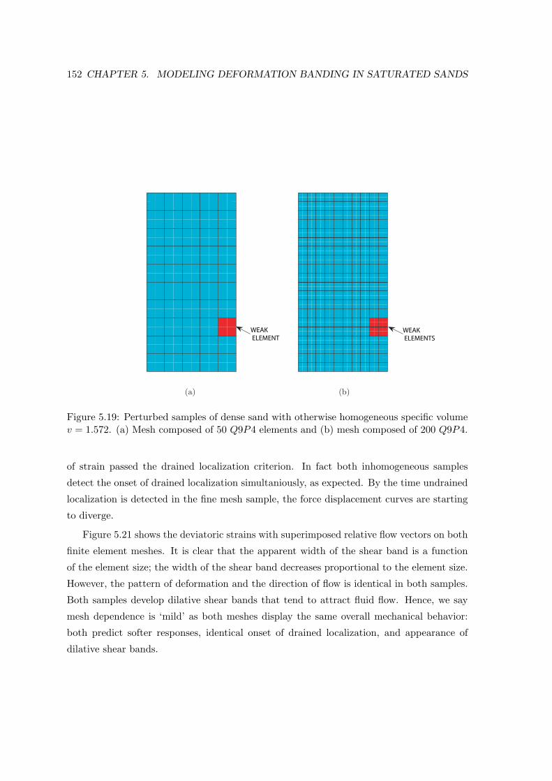
152 CHAPTER 5. MODELING DEFORMATION BANDING IN SATURATED SANDS
(a) (b)
WEAK
ELEMENTS
WEAK
ELEMENT
Figure 5.19: Perturbed samples of dense sand with otherwise homogeneous specific volumev = 1.572. (a) Mesh composed of 50 Q9P4 elements and (b) mesh composed of 200 Q9P4.
of strain passed the drained localization criterion. In fact both inhomogeneous samples
detect the onset of drained localization simultaniously, as expected. By the time undrained
localization is detected in the fine mesh sample, the force displacement curves are starting
to diverge.
Figure 5.21 shows the deviatoric strains with superimposed relative flow vectors on both
finite element meshes. It is clear that the apparent width of the shear band is a function
of the element size; the width of the shear band decreases proportional to the element size.
However, the pattern of deformation and the direction of flow is identical in both samples.
Both samples develop dilative shear bands that tend to attract fluid flow. Hence, we say
mesh dependence is ‘mild’ as both meshes display the same overall mechanical behavior:
both predict softer responses, identical onset of drained localization, and appearance of
dilative shear bands.

5.6. NUMERICAL SIMULATIONS 153
0 1 2 3 4 5 6100
120
140
160
180
200
220
240
260
280
NOMINAL AXIAL STRAIN, %
NO
MIN
AL
AX
IAL
ST
RE
SS
, k
Pa
INHOMOGENEOUS: 200 ELINHOMOGENEOUS: 50 EL
HOMOGENEOUS
DRAINED
LOCALIZATION
UNDRAINED LOCALIZATION
Figure 5.20: Force displacement curves comparing perfectly homogeneous response to thatof perturbed samples
0.025
0.03
0.035
0.04
0.045
0.05
0.055
0.06
0.065
0.07
0.025
0.03
0.035
0.04
0.045
0.05
0.055
(a) (b)
Figure 5.21: Deviatoric strains in contours with superimposed relative flow vectors q at 3%axial strain for (a) 50 element mesh and (b) 200 element mesh

154 CHAPTER 5. MODELING DEFORMATION BANDING IN SATURATED SANDS
5.7 Conclusion
We have presented a finite element model for the simulation of saturated porous media
exhibiting meso-scale inhomogeneities in the porosity field. The continuum balance laws
have been derived and utilized within a finite element framework from which the basic un-
knowns: solid displacements and Cauchy pore fluid pressures have been resolved in a u− p
mixed finite element scheme. The scheme features stable solutions with optimum rates of
convergence. Representative numerical examples dealing with plane strain compression of
undrained samples of dense and loose sands have been presented to underscore the im-
portance of meso-scale inhomogeneities on the stability and flow characteristics through a
deforming sand specimen. We have shown that behavior of saturated granular media is
more complex than that inferred from macroscopic observations and that even small im-
perfections at a scale smaller than specimen size can trigger global failure and influence
the amount and direction of flow. Furthermore, the behavior of relatively dense and loose
samples differ substantially as the volumetric behavior of the solid matrix is coupled with
the fluid flow, hence affecting the effective pressures, which govern strength in geomaterials.
These last observations are unique to this study in which porosity has been coupled with
the hydraulic conductivity and effective stress behavior of the underlying granular media,
thereby capturing both compactive and dilative modes of deformation banding.

Chapter 6
Conclusion and future work
We have proposed a meso-scale numerical model for predicting the location and direction of
deformation banding in saturated sands. A novel constitutive model for sands was developed
with the objective of capturing the most important features of sand behavior: nonlinear-
ity and irrecoverable deformations, pressure dependence, different strength under triaxial
compression/extension, relative density dependence, and nonassociative plastic flow. The
elastoplastic constitutive model developed herein uniquely captures all of these features and
is capable of accounting for spatial fluctuations in the porosity field, as measured, for exam-
ple, by X-Ray Computed Tomography. For sands, the meso-scale resolution of the porosity
field is in the millimeter scale. Motivated by the fact that CT technology can capture meso-
scale defects in samples of sand, we have demonstrated that these imperfections—though
small—must be taken into account when analyzing the behavior of sand specimens.
The meso-scale constitutive model was implemented in a nonlinear continuum mechan-
ics framework by designing a return mapping algorithm along the principal directions of
deformation. From the return mapping algorithm, the consistent tangent operator was
obtained in closed form and utilized in the finite element implementation of the model to
guarantee asymptotic quadratic rate of convergence. Numerical simulations at large strains
were performed for drained samples of dense sands under plane strain and triaxial condi-
tions. Both structured and unstructured porosity fields were used in the simulations. It
was concluded that the meso-scale inhomogeneities in the porosity consistently triggered
instabilities in the form of deformation bands. Localization was detected using a search
algorithm designed to exploit the spectral directions of the stress tensor, making the 3D
search very efficient.
155

156 CHAPTER 6. CONCLUSION AND FUTURE WORK
Comparisons between inhomogeneous samples and their homogeneous counterparts
showed that, after some axial deformation, the meso-scale inhomogeneities triggered insta-
bilities that were unique to the inhomogeneous samples. Consistently, homogeneous and
inhomogeneous samples predicted initially identical force-displacement curves, with homo-
geneous samples becoming stiffer after the inhomogeneities triggered softening and/or strain
localization in the perturbed samples. This last observation is critical as it shows that, since
the inhomogeneities do not influence the mechanical behavior of samples from the onset, it
is possible to calibrate the meso-scale model based on data from laboratory tests on ‘homo-
geneous’ specimens during the phase when the responses are identical. We plan to exploit
this nice feature in a subsequent calibration phase, where we will couple the model with
experimental results obtained in the laboratory.
The question of soil-fluid interaction and the effect of drainage has also been analyzed
in this dissertation against the backdrop of the proposed meso-scale constitutive model.
The mixture theory and nonlinear continuum mechanics have been invoked to derive the
balance laws governing the deformation-diffusion process in saturated bodies. A mixed
u − p formulation was developed to solve the balance laws in time and space. Numerical
simulations of plane strain compression under globally undrained conditions in samples of
loose and dense sands were conducted. Results were consistent with the findings under
drained conditions: meso-scale inhomogeneities (even small ones) trigger instabilities that
lead to the development of shear bands. These bands influence the flow characteristics in
the sample as they tend to attract flow in the case of dense sands but rather repel flow in
the case of loose sands. This is a direct consequence of the fact that dense sands behavior
is mostly dilative, whereas that of loose sands is mostly contractive. To the knowledge of
the author, all results reported in the literature show dilative shear bands attracting fluid
flow. This is the only work showing the effect of compactive shear bands repelling fluid
flow. This model is capable of capturing these effects because it accounts for the influence
of relative density explicitly as well as plastic dilation/compaction.
It is concluded that meso-scale inhomogeneities, which are inevitably present in ‘homo-
geneous’ samples of sand, play a crucial role in the mechanical behavior of specimens under
drained and undrained conditions at finite strains.
Possible improvements of this work include implementing the theory developed in Chap-
ter 5 in three dimensions. Even though the framework is fully three-dimensional, the numer-
ical examples are all in plane strain. It is necessary to implement the model utilizing brick

157
elements equipped with the mixed formulation. One has to be careful, however, as satisfac-
tion of the Babuska-Brezzi condition in 3D is not straight-forward. Therefore, development
of stabilized nonlinear finite elements may become necessary to avoid stability problems
associated with the deformation-diffusion problem near time t = 0+. Another possible
(and necessary) improvement of this work, is the use of enhanced elements to circumvent
the mesh dependence associated with the onset of strain localization. This improvement
would allow for a more robust post-localization simulation. Also, it is necessary to de-
velop and implement post-bifurcation constitutive models for sands to be able to simulate
post-localization behavior more realistically.
Development of meso-scale models based on particulate mechanics is also possible but
outside the scope of this dissertation. The approach here has been to develop a purely
continuum formulation including information at the meso-scale. One can imagine that a
multi-scale approach looking at the inter-particle behavior, and then transferring stress-
strain responses to the macro-scale or for calibrating the already existing meso-scale model
at the gauss points, is quite plausible. The effects of boundary conditions need also be
investigated. It is well know that the end platens in compression tests—even well lubricated
ones—introduce friction at the boundaries that makes the deformation inhomogeneous. It
is therefore necessary to incorporate these end constrains by using, for example, contact
elements to simulate the effect of friction from the platens.
The aspect of diffuse instabilities has been explicitly avoided in this dissertation but
should be studied in the near future as it could open doors to the understanding and
simulation of important instabilities mostly associated with loose sands. Diffuse instabilities
such as liquefaction must be studied in order to predict the catastrophic effects associated
with this phenomenon under fully dynamic excitations.

158 CHAPTER 6. CONCLUSION AND FUTURE WORK

Appendix A
Finite element u − p formulation
Equation (5.4.42) can be rewritten in indicial notation as
δg1 = ciA
∫
Ω0
[NA,j
(aepijkl + Jp (δilδjk − δijδkl)
)NB,lδdBk − JNA,iNBδpB
]dΩ0, (A.0.1)
following the notations in [119] (cf. equations (5.4.49) and (5.4.51)),
ui ≈∑
A∈η−ηd
NAdiA +∑
A∈ηd
N ξAξA (A.0.2)
p ≈∑
A∈η−ηp
NApA +∑
A∈ηp
N ζAζA (A.0.3)
ηi ≈∑
A∈η−ηd
NAciA (A.0.4)
ψ ≈∑
A∈η−ηp
NAcA (A.0.5)
where η and η denote the set of global node numbers for the displacement and pressure,
respectively. Similarly, we let ηd and ηp be the nodes at which the displacements and
pressures are prescribed, hence η−ηd and η−ηp represent the active sets for the displacement
and pressure, respectively. By the same token,
δg2 = −ciA∫
Ω0
JNAγfi
[NB,jδdjB +
φf
KfNBδpB
]dΩ0. (A.0.6)
159

160 APPENDIX A. MIXED FORMULATION
The linearized equations pertaining to the balance of mass equations can also be rewrit-
ten in indicial notation i.e.,
δh∆t1 = cA
∫
Ω0
JNAρf
[NB,jδdjB +
φf
KfNBδpB
]dΩ0, (A.0.7)
and
δh∆t2 =
α∆t
gcA
∫
Ω0
Jkij[NA,iNB,kδdkB −NA,kNB,iδdkB
](p,j − γfj) dΩ0
+α∆t
gcA
∫
Ω0
J
µNA,iδijk
′γf
(1 − φf
)NB,kδdkB (p,j − γfj) dΩ0
+α∆t
gcA
∫
Ω0
JNA,ikijKfNBδpB (p,j − γfj) dΩ0
+α∆t
gcA
∫
Ω0
JNA,ikij
[NB,jδpB − γfj
KfNBδpB − p,kNB,jδdkB
]dΩ0. (A.0.8)
From this point forward we adopt Voigt notation and hence, a fourth-order tensor α is
mapped into a 9 × 9 array i.e.,
α =
[αiikk][αii(kl)
] [αii[kl]
][α(ij)kk
] [α(ij)(kl)
] [α(ij)[kl]
][α[ij]kk
] [α[ij](kl)
] [α[ij][kl]
]
(no sum) (A.0.9)
where i, j, k, l = 1, 2, 3, and i 6= j and k 6= l. Also, each submatrix in square brackets
represents a 3 × 3 array. For example,
[α(ij)[kl]
]=
α(12)[12] α(12)[23] α(12)[31]
α(23)[12] α(23)[23] α(23)[31]
α(31)[12] α(31)[23] α(31)[31]
, (A.0.10)
where the parentheses signify a symmetric operator, whereas the square brackets signify a
skew-symmetric operator. For example,
α(12)[23] =1
4(α1223 − α1232 + α2123 − α2132) . (A.0.11)

161
Similarly, a second-order tensor ∇x η is mapped into a 9 × 1 vector i.e.,
∇x η =η1,1, η2,2, η3,3, 2η(1,2), 2η(2,3), 2η(3,1), 2η[1,2], 2η[2,3], 2η[3,1]
t(A.0.12)
such that the scalar product ηi,jαijklηk,l ≡ ∇x ηtα∇x η is recovered. Also, given the finite
element approximations in (5.4.51)1,2 we have
∇x η = Bc (A.0.13)
∇xψ = Γc, (A.0.14)
where B is the usual strain-displacement matrix i.e., B = [B1,B2, . . . ,Bnu], and
BA =
NA,1 0 0
0 NA,2 0
0 0 NA,3
NA,2 NA,1 0
0 NA,3 NA,2
NA,3 0 NA,1
NA,2 −NA,1 0
0 NA,3 −NA,2
−NA,3 0 NA,1
. (A.0.15)
By the same token, the matrix Γ = [Γ1,Γ2, . . . ,Γnp]. The components of Γ read
ΓA =NA,1, NA,2, NA,3
t. (A.0.16)
It is convenient at this point to introduce the following operators. Let a be a vector or
first-order tensor with components ai with i = 1, 2, 3, then let
ǫ (a) =
a1 0 0 12a2 0 1
2a312a2 0 −1
2a3
0 a2 0 12a1
12a3 0 −1
2a112a3 0
0 0 a3 0 12a2
12a1 0 −1
2a212a1
. (A.0.17)
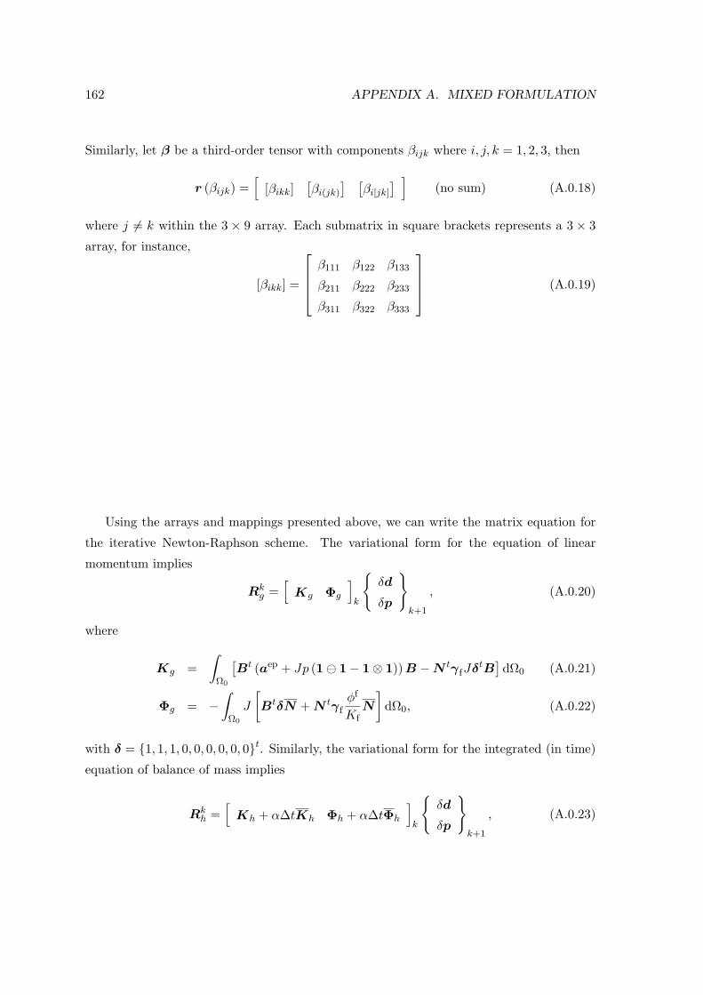
162 APPENDIX A. MIXED FORMULATION
Similarly, let β be a third-order tensor with components βijk where i, j, k = 1, 2, 3, then
r (βijk) =[
[βikk][βi(jk)
] [βi[jk]
] ](no sum) (A.0.18)
where j 6= k within the 3 × 9 array. Each submatrix in square brackets represents a 3 × 3
array, for instance,
[βikk] =
β111 β122 β133
β211 β222 β233
β311 β322 β333
(A.0.19)
Using the arrays and mappings presented above, we can write the matrix equation for
the iterative Newton-Raphson scheme. The variational form for the equation of linear
momentum implies
Rkg =
[Kg Φg
]
k
δd
δp
k+1
, (A.0.20)
where
Kg =
∫
Ω0
[Bt (aep + Jp (1 ⊖ 1 − 1 ⊗ 1))B − N tγfJδtB
]dΩ0 (A.0.21)
Φg = −∫
Ω0
J
[BtδN + N tγf
φf
KfN
]dΩ0, (A.0.22)
with δ = 1, 1, 1, 0, 0, 0, 0, 0, 0t. Similarly, the variational form for the integrated (in time)
equation of balance of mass implies
Rkh =
[Kh + α∆tKh Φh + α∆tΦh
]
k
δd
δp
k+1
, (A.0.23)

163
where
Kh =
∫
Ω0
NtJρfδ
tB dΩ0 (A.0.24)
Φh =
∫
Ω0
NtJρf
φf
KfN dΩ0 (A.0.25)
Kh =
∫
Ω0
J
gΓt[(
k +k′
µγf
(1 − φf
)1
)· (∇x pf − γf)
]δtB dΩ0
−∫
Ω0
J
gΓt [ǫ (k · (∇x p− γf)) + r (kikp,j)]BdΩ0 (A.0.26)
Φh =
∫
Ω0
J
gΓtk
[1
Kf(∇x p− γf)N + Γ
]dΩ0, (A.0.27)
and hence the incremental solution in equation (5.4.57).

164 APPENDIX A. MIXED FORMULATION

Bibliography
[1] G. T. Houlsby. The use of a variable shear modulus in elasto-plastic models for clays.
Computers and Geotechnics, 1:3–13, 1985.
[2] M. G. Jefferies. Nor-Sand: a simple critical state model for sand. Geotechnique,
43:91–103, 1993.
[3] S. L. Kramer. Geotechnical Earthquake Engineering. Prentice-Hall, New Jersey, 1996.
[4] K. A. Alshibli, S. N. Batiste, and S. Sture. Strain localization in sand: plane strain
versus triaxial compression. Journal of Geotechnical and Geoenvironmental Engineer-
ing, ASCE, 129:483–494, 2003.
[5] A. J. Durrani, A. S. Elnashai, Y. M. A. Hashash, S. J. Kim, and A. Masud. The
Kashmir earthquake of October 8, 2005. A quick look report. Technical Report 05-04,
Mid-America Earthquake Center, 2005.
[6] A. Schofield and P. Wroth. Critical State Soil Mechanics. McGraw-Hill, New York,
1968.
[7] J. Graham, J. H. A. Crooks, and A. L. Bell. Yield states and stress–strain behaviour
of natural soft clays. Canadian Geotechnical Journal, 20:502–516, 1983.
[8] P. V. Lade and J. M. Duncan. Elastoplastic stress-strain theory for cohesionless soil.
Journal of the Geotechnical Engineering Division, ASCE, 101:1037–1053, 1975.
[9] D. H. Cornforth. Some experiments on the influence of strain conditions on the
strength of sand. Geotechnique, 14:143–167, 1964.
[10] H. B. Poorooshasb, I. Holubec, and A. N. Sherbourne. Yielding and flow of sand in
triaxial compression: Part I. Canadian Geotechnical Journal, 3:179–190, 1966.
165

166 BIBLIOGRAPHY
[11] H. B. Poorooshasb, I. Holubec, and A. N. Sherbourne. Yielding and flow of sand in
triaxial compression: Parts II and III. Canadian Geotechnical Journal, 4:376–397,
1967.
[12] A. Aydin. Fractures, faults, and hydrocarbon entrapment, migration and flow. Marine
and Petroleum Geology, 17:797–814, 2000.
[13] G. Castro. Liquefaction of sands. Harvard University, Harvard Soil Mechanics Series
81, Jan 1969.
[14] K. Ishihara. Liquefaction and flow failure during earthquakes. Geotechnique, 43:351–
415, 1993.
[15] J. Desrues, R. Chambon, M. Mokni, and F. Mazerolle. Void ratio evolution in-
side shear bands in triaxial sand specimens studied by computed tomography.
Geotechnique, 46:527–546, 1996.
[16] L. B. Wang, J. D. Frost, and J. S. Lai. Three-dimensional digital representation
of granular material microstructure from X-Ray tomography imaging. Journal of
Computing in Civil Engineering, ASCE, 18:28–35, 2004.
[17] P. Wriggers and S. O. Moftah. Mesoscale models for concrete: Homogenisation and
damage behaviour. Finite Elements in Analysis and Design, 42:623–636, 2006.
[18] S. Hafner, S. Eckardt, T. Luther, and C. Konke. Mesoscale modeling of concrete:
Geometry and numerics. Computers & Structures, 84:450–461, 2006.
[19] K. Nubel and W. Huang. A study of localized deformation pattern in granular media.
Computer Methods in Applied Mechanics and Engineering, 193:2719–2743, 2004.
[20] M. Mokni and J. Desrues. Strain localization measurements in undrained plane-strain
biaxial tests on hostun rf sand. Mechanics of Cohesive-Frictional Materials, 4:419–
441, 1998.
[21] C. Han and G. Vardoulakis. Plane-strain compression experiments on water-saturated
fine-grained sand. Geotechnique, 41:49–78, 1991.
[22] R. J. Finno, W. W. Harris, M. A. Mooney, and G. Viggiani. Shear bands in plane
strain compression of loose sand. Geotechnique, 47:149–165, 1997.

BIBLIOGRAPHY 167
[23] R. J. Finno, D. K. Atmatzidis, and S. B. Perkins. Observed performance of deep a
excavation in clay. Journal of Geotechnical Engineering, ASCE, 115:1045–1064, 1989.
[24] R. J. Finno and S. M. Nerby. Saturated clay response during braced cut construction.
Journal of Geotechnical Engineering, ASCE, 115:1065–1084, 1989.
[25] J. Hadamard. Lecons sur la propagation des ondes et les equations de
l’hydrodynamique. Librarie Scientifique A, Paris, 1903.
[26] R. Hill. A general theory of uniqueness and stability in elastic-plastic solids. Journal
of the Mechanics and Physics of Solids, 6:236–249, 1958.
[27] T. Thomas. Plastic Flow and Fracture in Solids. Academic Press, New York, NY,
1961.
[28] J. Mandel. Conditions de stabilite et postulat de Druker. In J. Kravtchenko and P. M.
Sirieys, editors, Rheology and Soil Mechanics. Springer, 1966.
[29] J. W. Rudnicki and J. R. Rice. Conditions for localization of deformation in pressure-
sensitive dilatant materials. Journal of the Mechanics and Physics of Solids, 23:371–
394, 1975.
[30] J. E. Marsden and T. J. R. Hughes. Mathematical Theory of Elasticity. Prentice-Hall,
Englewood Cliffs, NJ, 1983.
[31] J. C. Simo, J. Oliver, and F. Armero. An analysis of strong discontinuities induced
by strain-softening in rate-independent inelastic solids. Computational Mechanics,
12:277–296, 1993.
[32] M. Ortiz. An analytical study of the localized failure modes of concrete. Mechanics
of Materials, 6:159–174, 1987.
[33] D. Bigoni and T. Hueckel. Uniqueness and localization—i. Associative and non-
associative elastoplasticity. International Journal for Solids and Structures, 28:197–
213, 1991.
[34] K. Runesson, N. S. Ottosen, and D. Peric. Discontinuous bifurcations of elastic-
plastic solutions at plane stress and plane strain. International Journal of Plasticity,
7:99–121, 1991.

168 BIBLIOGRAPHY
[35] N. S. Ottosen and K. Runesson. Properties of discontinuous bifurcation solutions in
elasto-plasticity. International Journal of Solids and Structures, 27:401–421, 1991.
[36] M. K. Neilsen and H. L. Schreyer. Bifurcations in elastic-plastic materials. Interna-
tional Journal for Solids and Structures, 30:521–544, 1993.
[37] D. Bigoni and D. Zaccaria. On strain localization analysis of elastoplastic materials
at finite strains. International Journal of Plasticity, 9:21–33, 1993.
[38] L. Szabo. Shear band formulations in finite strain elastoplasticity. International
Journal for Solids and Structures, 31:1291–1308, 1994.
[39] J. Desrues R. Chambon, S. Crochepeyre. Localization criteria for non-linear constitu-
tive equations of geomaterials. Mechanics of Cohesive-Frictional Materials, 5:61–82,
2000.
[40] W. A. Olsoon and D. J. Holcomb. Compaction localization in porous rock. Geophysical
Research Letters, 27:3537–3540, 2000.
[41] K. A. Issen and J. W. Rudnicki. Conditions for compaction bands in porous rock.
Journal of Geophysical Research, 105:21529–21536, 2000.
[42] J. W. Rudnicki. Shear and compaction band formation on an elliptic yield cap. Journal
of Geophysical Research, 109:1–10, 2004.
[43] R. I. Borja and A. Aydin. Computational modeling of deformation bands in granular
media. I. Geological and mathematical framework. Computer Methods in Applied
Mechanics and Engineering, 193:2667–2698, 2004.
[44] J. W. Rudnicki. Formulation for studying coupled deformation pore fluid diffusion
effects on localization of deformation. AMD (Symposia Series) (American Society of
Mechanical Engineers, Applied Mechanics Division), 57:35–44, 1983.
[45] R. Larsson, K. Runesson, and S. Sture. Embedded localization band in undrained
soil based on regularized strong discontinuity—theory and fe-analysis. International
Journal of Solids and Structures, 33:3081–3101, 1996.
[46] R. I. Borja. Cam-Clay plasticity, Part V: A mathematical framework for three-phase
deformation and strain localization analyses of partially saturated porous media. Com-
puter Methods in Applied Mechanics and Engineering, 193:5301–5338, 2004.

BIBLIOGRAPHY 169
[47] C. Callari and F. Armero. Analysis and numerical simulation of strong disconti-
nuities in finite strain poroplasticity. Computer Methods in Applied Mechanics and
Engineering, 193:2941–2986, 2004.
[48] I. Vardoulakis. Deformation of water-saturated sand: I. uniform undrained deforma-
tion and shear banding. Geotechnique, 46:441–456, 1996.
[49] I. Vardoulakis. Deformation of water-saturated sand: II. effect of pore water flow and
shear banding. Geotechnique, 46:457–472, 1996.
[50] J. H. Prevost. Localization of deformations in elastic-plastic solids. International
Journal for Numerical and Analytical Methods in Geomechanics, 8:187–196, 1984.
[51] M. Ortiz, Y. Leroy, and A. Needleman. A finite element method for localized failure
analysis. Computer Methods in Applied Mechanics and Engineering, 61:189–214, 1987.
[52] Y. Leroy and M. Ortiz. Finite element analysis of strain localization in frictional ma-
terials. International Journal for Numerical and Analytical Methods in Geomechanics,
13:53–74, 1989.
[53] Z. Bazant, T. Belytschko, and T. P. Chang. Continuum theory for strain-softening.
Journal of Engineering Mechanics, ASCE, 110:1666–1692, 1984.
[54] J. H. Prevost and B. Loret. Dynamic strain localization in elasto-(visco-)plastic solids,
part 1. General formulation and one-dimensional examples. Computer Methods in
Applied Mechanics and Engineering, 83:275–294, 1990.
[55] J. H. Prevost and B. Loret. Dynamic strain localization in elasto-(visco-)plastic solids,
part 2. Plane strain examples. Computer Methods in Applied Mechanics and Engi-
neering, 83:275–294, 1990.
[56] H. B. Muhlhaus and I. Vardoulakis. The thickness of shear bands in granular materials.
Geotechnique, 37:271–283, 1987.
[57] X. Li and H. Tang. A consistent return mapping algorithm for pressure-dependent
elastoplastic Cosserat continua and modelling of strain localization. Computers &
Structures, 83:1–10, 2005.

170 BIBLIOGRAPHY
[58] F. Armero and K. Garikipati. An analysis of strong discontinuities in multiplicative
finite strain plasticity and their relation with the numerical simulation of strain lo-
calization in solids. International Journal for Solids and Structures, 33:2863–2885,
1996.
[59] R. Larsson and K. Runesson. Element-embedded localization band based on regular-
ized displacement discontinuity. Journal of Engineering Mechanics, ASCE, 122:402–
411, 1996.
[60] R. A. Regueiro and R. I. Borja. A finite element model of localized deformation
in frictional materials taking a strong discontinuity approach. Finite Elements in
Analysis and Design, 33:283–315, 1999.
[61] R. I. Borja. A finite element model for strain localization analysis of strongly dis-
continuous fields based on standard Galerkin approximation. Computer Methods in
Applied Mechanics and Engineering, 190:1529–49, 2000.
[62] R. I. Borja and R. A. Regueiro. Strain localization in frictional materials exhibit-
ing displacement jumps. Computer Methods in Applied Mechanics and Engineering,
190:2555–2580, 2001.
[63] R. A. Regueiro and R. I. Borja. Plane strain finite element analysis of pressure sensitive
plasticity with strong discontinuity. International Journal of Solids and Structures,
38:3647–3672, 2001.
[64] R. I. Borja. Bifurcation of elastoplastic solids to shear band mode at finite strains.
Computer Methods in Applied Mechanics and Engineering, 191:5287–5314, 2002.
[65] K. H. Roscoe and J. H. Burland. On the generalized stress–strain behavior of ‘wet’
clay. In J. Heyman and F. A. Leckie, editors, Engineering Plasticity, pages 535–609.
Cambridge University Press, 1968.
[66] R. I. Borja and C. Tamagnini. Cam-Clay plasticity, Part III: Extension of the in-
finitesimal model to include finite strains. Computer Methods in Applied Mechanics
and Engineering, 155:73–95, 1998.
[67] R. Nova and D. M. Wood. A constitutive model for sand in triaxial compression.

BIBLIOGRAPHY 171
International Journal for Numerical and Analytical Methods in Geomechanics, 3:255–
278, 1979.
[68] M. Pastor, O. C. Zienkiewicz, and A. H. C. Chan. Generalized plasticity and the mod-
eling of soil behaviour. International Journal for Numerical and Analytical Methods
in Geomechanics, 14:151–190, 1990.
[69] J. M. Pestana and A. J. Whittle. Formulation of a unified constitutive model for
clays and sands. International Journal for Numerical and Analytical Methods in
Geomechanics, 23:1215–1243, 1999.
[70] H. Matsuoka and T. Nakai. A new failure criterion for soils in three-dimensional
stresses. In Conference on Deformation and Failure of Granular Materials, pages
253–263. IUTAM, 1982.
[71] P. V. Lade and M. K. Kim. Sigle hardening constitutive model for frictional materials
II. Yield criterion and plastic work contours. Computers and Geotechnics, 6:13–29,
1988.
[72] D. Peric and M.A. Ayari. Influence of Lode’s angle on the pore pressure generation
in soils. International Journal of Plasticity, 18:1039–1059, 2002.
[73] D. Peric and M.A. Ayari. On the analytical solutions for the three-invariant Cam clay
model. International Journal of Plasticity, 18:1061–1082, 2002.
[74] R. D. Holtz and W. D. Kovacs. An Introduction to Geotechnical Engineering. Prentice-
Hall, Inc., Englewood Cliffs, NJ, 1981.
[75] M. T. Manzari and Y. F. Dafalias. A critical state two-surface plasticity model for
sands. Geotechnique, 43:255–272, 1997.
[76] N. Khalili, M. A. Habte, and S. Valliappan. A bounding surface plasticity model
for cyclic loading of granular soils. International Journal for Numerical Methods in
Engineering, 63:1939–1960, 2005.
[77] R. Nova. The role of non-normality in soil mechanics and some of its mathematical
consequences. Computers and Geotechnics, 31:185–191, 2004.

172 BIBLIOGRAPHY
[78] K. A. Alshibli, S. Sture, N. C. Costes, M. L. Frank, F. R. Lankton, S. N. Batiste, and
R. A. Swanson. Assessment of localized deformations in sand using x-ray computed
tomography. Geotechnical Testing Journal, ASCE, 23:274–299, 2000.
[79] K. A. Alshibli and S. Sture. Shear band formation in plane strain compression. Journal
of Geotechnical and Geoenvironmental Engineering, ASCE, 126:495–503, 2000.
[80] J. Desrues and G. Viggiani. Strain localization in sand: an overview of the experimen-
tal results obtained in grenoble using stereophotogrammetry. International Journal
for Numerical and Analytical Methods in Geomechanics, 28:279–321, 2004.
[81] R. J. Finno, W. W. Harris, and M. A. Mooney. Strain localization and undrained
steady state of sands. Journal of Geotechnical Engineering, ASCE, 122:462–473, 1996.
[82] G. Gudehus and K. Nubel. Evolution of shear bands in sand. Geotechnique, 54:187–
201, 2004.
[83] A. L. Rechenmacher and R. J. Finno. Digital image correlation to evaluate shear
banding in dilative sands. Geotechnical Testing Jounal, ASCE, 27:1–10, 2004.
[84] A. L. Rechenmacher and R. J. Finno. Shear band displacements and void ratio
evolution to critical state in dilative sands. In J. F. Labuz and A. Drescher, editors,
Bifurcation and Instabilities in Geomaterials, pages 13–22. A. A. Blakema Publishers,
2003.
[85] I. Vardoulakis, M. Goldscheider, and G. Gudehus. Formation of shear bands in sand
bodies as a bifurcation problem. International Journal for Numerical and Analytical
Methods Geomechanics, 2:99–128, 1978.
[86] I. Vardoulakis and B. Graf. Calibration of constitutive models for granular materials
using data from biaxial experiments. Geotechnique, 35:299–317, 1985.
[87] E. Bauer, W. Wu, and W. Huang. Influence of an initially transverse isotropy on shear
banding in granular materials. In J. F. Labuz and A. Drescher, editors, Bifurcation
and Instabilities in Geomaterials, pages 161–172. A. A. Blakema Publishers, 2003.
[88] R. I. Borja and T. Y. Lai. Propagation of localization instability under active and
passive loading. Journal of Geotechnical and Geoenvironmental Engineering, ASCE,
128:64–75, 2002.

BIBLIOGRAPHY 173
[89] R. Chambon and J. C. Moullet. Uniqueness studies in boundary value problems
involving some second gradient models. Computer Methods in Applied Mechanics and
Engineering, 193:2771–2796, 2004.
[90] R. Chambon, D. Caillerie, and C. Tamagnini. A strain space gradient plasticity
theory for finite strain. Computer Methods in Applied Mechanics and Engineering,
193:2797–2826, 2004.
[91] F. Darve, G. Servant, F. Laouafa, and H. D. V. Khoa. Failure in geomaterials: contin-
uous and discrete analyses. Computer Methods in Applied Mechanics and Engineering,
193:3057–3085, 2004.
[92] R. de Borst and H. B. Muhlhaus. Gradient-dependent plasticity: Formulation and
algorithmic aspects. International Journal for Numerical Methods in Engineering,
35:521–539, 1992.
[93] A. Gajo, D. Bigoni, and D. M. Wood. Stress induced elastic anisotropy and strain
localisation in sand. In H. B. Muhlhaus, A. Dyskin, and E. Pasternak, editors, Bifur-
cation and Localisation Theory in Geomechanics, pages 37–44. A. A. Blakema Pub-
lishers, 2001.
[94] S. Kimoto, F. Oka, and Y. Higo. Strain localization analysis of elasto-viscoplastic
soil considering structural degradation. Computer Methods in Applied Mechanics and
Engineering, 193:2845–2866, 2004.
[95] P. A. Klerck, E. J. Sellers, and D. R. J. Owen. Discrete fracture in quasi-brittle
materials under compressive and tensile stress states. Computer Methods in Applied
Mechanics and Engineering, 193:3035–3056, 2004.
[96] B. Muhunthan, O. Alhattamleh, and H. M. Zbib. Modeling of localization in gran-
ular materials: effect of porosity and particle size. In J. F. Labuz and A. Drescher,
editors, Bifurcation and Instabilities in Geomaterials, pages 121–131. A. A. Blakema
Publishers, 2003.
[97] E. Onate and J. Rojek. Combination of discrete element and finite element methods for
dynamic analysis of geomechanics problems. Computer Methods in Applied Mechanics
and Engineering, 193:3087–3128, 2004.
174 BIBLIOGRAPHY
[98] M. Ortiz and A. Pandolfi. A variational cam-clay theory of plasticity. Computer
Methods in Applied Mechanics and Engineering, 193:2645–2666, 2004.
[99] M. R. Salari, S. Saeb, K. J. Willam, S. J. Patchet, and R. C. Carrasco. A coupled
elastoplastic damage model for geomaterials. Computer Methods in Applied Mechanics
and Engineering, 193:2625–2643, 2004.
[100] J. Tejchman and G. Gudehus. Shearing of a narrow granular layer with polar quan-
tities. International Journal for Numerical and Analytical Methods in Geomechanics,
25:1–28, 2001.
[101] I. Vardoulakis, E. Vairaktaris, and E. Papamichos. Subsidence diffusion-convection:
I. the direct problem. Computer Methods in Applied Mechanics and Engineering,
193:2745–2760, 2004.
[102] R. G. Wan and P. J. Guo. Constitutive modelling of granular materials with focus to
microstructure and its effect on strain localization. In J. F. Labuz and A. Drescher,
editors, Bifurcation and Instabilities in Geomaterials, pages 149–160. A. A. Blakema
Publishers, 2003.
[103] Z. Q. Yue, S. Chen, and L. G. Tham. Finite element modeling of geomaterials using
digital image processing. Computers and Geotechnics, 30:375–397, 2003.
[104] R. I. Borja and S. R. Lee. Cam-Clay plasticity, Part I: Implicit integration of elasto-
plastic constitutive relations. Computer Methods in Applied Mechanics and Engineer-
ing, 78:49–72, 1990.
[105] R. I. Borja. Cam-Clay plasticity, Part II: Implicit integration of constitutive equation
based on nonlinear elastic stress predictor. Computer Methods in Applied Mechanics
and Engineering, 88:225–240, 1991.
[106] K. Been and M. G. Jefferies. A state parameter for sands. Geotechnique, 35:99–112,
1985.
[107] K. Ishihara, F. Tatsuoka, and S. Yasuda. Undrained deformation and liquefaction of
sand under cyclic stresses. Soils and Foundations, 15:29–44, 1975.
[108] A. Gens and D.M. Potts. Critical state models in computational geomechanics. En-
gineering Computations, 5:178–197, 1988.

BIBLIOGRAPHY 175
[109] R. J. Jardine, D. M. Potts, A. B. Fourie, and J. B. Burland. Studies of the influence
of non-linear stress-strain characteristics in soil-structure interaction. Geotechnique,
36:377–396, 1986.
[110] P. V. Lade. Static instability and liquefaction of loose fine sandy slopes. Journal of
Geotechnical Engineering, ASCE, 118:51–71, 1992.
[111] R. I. Borja, K. M. Sama, and P. F. Sanz. On the numerical integration of three-
invariant elastoplastic constitutive models. Computer Methods in Applied Mechanics
and Engineering, 192:1227–1258, 2003.
[112] J. C. Simo and T. J. R. Hughes. Computational Inelasticity. Prentice-Hall, New York,
1998.
[113] J. Sulem, I. Vardoulakis, E. Papamichos, A. Oulahna, and J. Tronvoll. Elasto-plastic
modelling of red wildmoor sandstone. Mechanics of Cohesive-Frictional Materials,
4:215–245, 1999.
[114] R. I. Borja. Computational modeling of deformation bands in granular media. II.
Numerical simulations. Computer Methods in Applied Mechanics and Engineering,
193:2699–2718, 2004.
[115] E. H. Lee. Elastic-plastic deformation at finite strain. Journal of Applied Mechanics,
36:1–6, 1969.
[116] L. E. Malvern. Introduction to the Mechanics of a Continuous Medium. Prentice-Hall,
Inc., Englewood Cliffs, NJ, 1969.
[117] J. C. Simo. Algorithms for static and dynamic multiplicative plasticity that preserve
the classical return mapping schemes of the infinitesimal theory. Computer Methods
in Applied Mechanics and Engineering, 99:61–112, 1992.
[118] Y. F. Dafalias. Plastic spin: necessity or redundancy? International Journal of
Plasticity, 14:909–931, 1998.
[119] T. J. R. Hughes. The Finite Element Method. Prentice-Hall, Englewood Cliffs, NJ,
1987.

176 BIBLIOGRAPHY
[120] J. C. Nagtegaal, D. M. Parks, and J. R. Rice. On numerically accurate finite element
solutions in the fully plastic regime. Computer Methods in Applied Mechanics and
Engineering, 4:153–177, 1974.
[121] J. C. Simo, R. L. Taylor, and K. S. Pister. Variational and projection methods for
the volume constraint in finite deformation elasto-plasticity. Computer Methods in
Applied Mechanics and Engineering, 51:177–208, 1985.
[122] R. I. Borja and J. E. Andrade. Critical state plasticity, Part VI: Meso-scale finite
element simulation of strain localization in discrete granular materials. Computer
Methods in Applied Mechanics and Engineering, 2006. In press for the John Argyris
Memorial Special Issue.
[123] W. Lode. Versuche ueber den einfluss der mitt leren Hauptspannung auf das Fliessen
der Metalle Eisen Kupfer und Nickel. Zeitschrift fuer Physik, 36:913–939, 1926.
[124] G. A. Holzapfel. Nonlinear Solid Mechanics. John Wiley & Sons Ltd, West Sussex,
UK, 2000.
[125] R. I. Borja, C. Tamagnini, and A. Amorosi. Coupling plasticity and energy-conserving
elasticity models for clays. Journal of Geotechnical and Geoenvironmental Engineer-
ing, ASCE, 123:948–957, 1997.
[126] R. I. Borja. Plasticity modeling and computation. Lecture Notes, Stanford University,
California, 2005.
[127] G. Gudehus. Elastoplastische stoffgleichungen fur trockenen sand. Ingenieur-Archiv,
42:151–169, 1973.
[128] J. H. Argyris, G. Faust, J. Szimmat, E. P. Warnke, and K. J. Willam. Recent devel-
opments in the finite element analysis of prestressed concrete reactor vessels. Nuclear
Engineering and Design, 28:42–75, 1974.
[129] J. Jiang and Pietruszczak. Convexity of yield loci for pressure sensitive materials.
Computers and Geotechnics, 5:51–63, 1988.
[130] K. J. Willam and E. P. Warnke. Constitutive model for the triaxial behaviour of
concrete. In Concrete Structures Subjected to Triaxial Stresses, Bergamo, Italy, May
1974. ISMES.

BIBLIOGRAPHY 177
[131] J. E. Andrade and R. I. Borja. Fully implicit numerical integration of a hypere-
lastoplastic model for sands based on critical state plasticity. In K. J. Bathe, editor,
Computational Fluid and Solid Mechanics 2005, pages 52–54. Elsevier Science Ltd.,
2005.
[132] J. Bonet and R. D. Wood. Nonlinear Continuum Mechanics for for Finite Element
Analysis. Cambridge University Press, Cambridge, UK, 1997.
[133] T. Belytschko, W. K. Liu, and B. Moran. Nonlinear Finite Elements for Continua
and Structures. John Wiley & Sons Ltd., West Sussex, UK, 2000.
[134] M. Ortiz and J. B. Martin. Symmetry-preserving return mapping algorithms and
incrementally extremal paths - a unification of concepts. International Journal for
Numerical Methods in Engineering, 8:1839–1853, 1989.
[135] K. Willam. Constitutive models for engineering materials. In Encyclopedia of Physical
Science and Technology, volume 3. Academic Press, third edition, 2002.
[136] J. Oliver and A. E. Huespe. Theoretical and computational issues in modeling material
failure in strong discontinuity scenarios. Computer Methods in Applied Mechanics and
Engineering, 193:2987–3014, 2004.
[137] J. Mosler. Numerical analyses of discontinuous material bifurcation: strong and weak
discontinuities. Computer Methods in Applied Mechanics and Engineering, 194:979–
1000, 2005.
[138] M. Shahinpoor. Statistical mechanical considerations on the random packing of gran-
ular materials. Powder Technology, 25:163–176, 1980.
[139] J. R. Benjamin and C. A. Cornell. Probability, Statistics, and Decision for Civil
Engineers. McGraw-Hill, Inc., New York, 1970.
[140] T. Y. Lai, R. I. Borja, B. G. Duvernay, and R. L. Meehan. Capturing strain localiza-
tion behind a geosynthetic-reinforced soil wall. International Journal for Numerical
and Analytical Methods in Geomechanics, 27:425–451, 2003.
[141] J. R. Rice. On the stability of dilatant hardening for saturated rock masses. Journal
of Geophysical Research, 80:1531–1536, 1975.

178 BIBLIOGRAPHY
[142] J. W. Rudnicki. Effects of dilatant hardening on the development of concentrated
shear deformation in fissured rock masses. Journal of Geophysical Research, 89:9259–
9270, 1984.
[143] F. Armero. Formulation and finite element implementation of multiplicative model of
coupled poro-plasticity at finite strains under fully saturated conditions. Computer
Methods in Applied Mechanics and Engineering, 171:205–241, 1999.
[144] J. Larsson and R. Larsson. Non-linear analysis of nearly saturated porous media:
theoretical and numerical formulation. Computer Methods in Applied Mechanics and
Engineering, 191:3885–3907, 2002.
[145] B. A. Schrefler, H. W. Zhang, M. Pastor, and O. C. Zienkiewicz. Strain localisation
modeling and pore pressure in saturated sand samples. Computational Mechanics,
22:266–280, 1998.
[146] W. Ehlers, T. Graf, and M. Ammann. Deformation and localization analysis of
partially saturated soil. Computer Methods in Applied Mechanics and Engineering,
193:2885–2910, 2004.
[147] B. Loret and J. H. Prevost. Dynamic strain localization in fuid-saturated porous
media. Journal of Engineering Mechanics, ASCE, 117:907–922, 1991.
[148] B. A. Schrefler, L. Sanavia, and C. E. Majorana. A multiphase medium model for
localisation and postlocalisation simulation in geomaterials. Mechanics of Cohesive-
Frictional Materials, 1:95–114, 1996.
[149] H. W. Zhang, L. Sanavia, and B. A. Schrefler. An internal lenght scale in dynamic
strain localization of multiphase porous media. Mechanics of Cohesive-Frictional
Materials, 4:443–460, 1999.
[150] P. Steinmann. A finite element formulation for strong discontinuities in fluid-saturated
porous media. Mechanics of Cohesive-Frictional Materials, 4:133–152, 1999.
[151] A. L. Rechenmacher. Grain-scale processes governing shear band initiation and evo-
lution in sands. Journal of the Mechanics and Physics of Solids, 54:22–45, 2006.

BIBLIOGRAPHY 179
[152] J. E. Andrade and R. I. Borja. Capturing strain localization in dense sands with
random density. International Journal for Numerical Methods in Engineering, in
press, 2006.
[153] D. M. Wood. Soil Behaviour and Critical State Soil Mechanics. Cambridge University
Press, Cambridge, UK, 1990.
[154] R. M. Bowen. Theory of mixtures. In A. C. Eringen, editor, Continuum Physics,
volume III—Mixtures and EM Field Theories, New York, NY, 1976. Academic Press.
[155] R. J. Atkin and R. E. Craine. Continuum theories of mixture: basic theory and
historical development. Quarterly Journal of Mechanics and Applied Mathematics,
29:209–244, 1976.
[156] C. Li, R. I. Borja, and R. A. Regueiro. Dynamics of porous media at finite strain.
Computer Methods in Applied Mechanics and Engineering, 193:3837–3870, 2004.
[157] F. Armero and C. Callari. An analysis of strong discontinuities in a saturated poro-
plastic solid. International Journal for Numerical Methods in Engineering, 46:1673–
1698, 1999.
[158] J. Bear. Dynamics of Fluids in Porous Media. American Elsevier Publishing Company,
Inc., New York, NY, 1972.
[159] O. C. Zienkiewicz and R. L. Taylor. The Finite Element Method, volume 1.
Butterworth-Heinemann, Oxford, UK, fifth edition, 2000.
[160] J. H. Prevost. Mechanics of continuous porous media. International Journal of Engi-
neering Science, 18:787–800, 1980.
[161] O. Coussy. Mechanics of Porous Continua. John Wiley & Sons Ltd, West Sussex,
UK, 1995.
[162] A. Nur and J. D. Byerlee. An exact effective stress law for elastic deformation of rock
with fluids. Journal of Geophysical Research, 76:6414–6419, 1971.
[163] R. I. Borja. On the mechanical energy and effective stress in saturated and unsaturated
porous continua. International Journal of Solids and Structures, 43:1764–1786, 2006.

180 BIBLIOGRAPHY
[164] K. Terzaghi. Theoretical Soil Mechanics. John Wiley & Sons Ltd, New York, NY,
1943.
[165] P. Pivonka and K. Willam. The effect of the third invariant in computational plasticity.
Engineering Computations, 20:741–753, 2003.
[166] O. C. Zienkiewicz, A. H. C. Chan, M. Pastor, B. A. Schrefler, and T. Shiomi. Com-
putational Geomechanics. John Wiley & Sons Ltd, New York, NY, 1999.
[167] J. Kozeny. Uber kapillare Leitung des Wassers im Boden. Sitzungsberichte der Kaiser-
lichen Akademie der Wissenschaften in Wien, 136:271–306, 1927.
[168] P. C. Carman. Fuid flow through a granular bed. Transactions of the Institution of
Chemical Engineers of London, 15:150–156, 1937.
[169] R. I. Borja and E. Alarcon. A mathematical framework for finite strain elastoplastic
consolidation Part 1: Balance laws, variational formulation, and linearization. Com-
puter Methods in Applied Mechanics and Engineering, 122:145–171, 1995.
[170] M. A. Murad and A. F. D. Loula. Improved accuracy in finite element analysis of Biot’s
consolidation problem. Computer Methods in Applied Mechanics and Engineering,
95:359–382, 1992.
[171] J. Wan. Stabilized Finite Element Methods for Coupled Geomechanics and Multiphase
Flow. PhD thesis, Stanford University, Stanford, CA, 2002.
[172] M. A. Murad and A. F. D. Loula. On stability and convergence of finite element
approximations of Biot’s consolidation problem. International Journal for Numerical
Methods in Engineering, 37:645–667, 1994.
[173] T. J. R. Hughes, L. P. Franca, and M. Balestra. A new finite element formulation
for computational fluid dynamics: V. Circumvemting the Babuska-Brezzi condition.
Computer Methods in Applied Mechanics and Engineering, 59:85–99, 1986.
[174] P. Mira, M. Pastor, T. Li, and X. Liu. A new stabilized enhanced strain element
with equal order of interpolation for soil consolidation problems. Computer Methods
in Applied Mechanics and Engineering, 192:4257–4277, 2003.

BIBLIOGRAPHY 181
[175] J. C. Simo and M. S. Rifai. A class of mixed assumed strain methods and the method
of incompatible modes. International Journal for Numerical Methods in Engineering,
29:1595–1638, 1990.
[176] H. W. Zhang and B. A. Schrefler. Particular aspects of internal lenght scales in strain
localization analysis of multiphase porous materials. Computer Methods in Applied
Mechanics and Engineering, 193:2867–2884, 2004.