Melt Pool Image Process Acceleration Using General PurposeComputing On Graphics Processing Units.

R. Sampson∗†, R. Lancaster∗, M. Weston†

∗ Institure of Structural Materials, Swansea University, United Kingdom, SA1 8EN† TWI Technology Centre, United Kingdom, SA13 1SB

June 16, 2017

Abstract

The additive manufacturing (AM) process is incredibly complex, and the intricate web of chang-ing process parameters can result in poor repeatability and structural consistency. New geomet-ric designs result in an initial iteration process to optimise build parameters, which is highlylaborious and time consuming. A deep understanding of process parameters in AM, and theability to control and manipulate said parameters, may lead to advanced AM capabilities.

Non-contact devices are typically required to measure the build characteristics such as meltpool geometry and temperature, which give a greater understanding of the complex AM pro-cess. This paper will look to view the molten metal pool that is formed in the Direct EnergyDeposition (DED) process using complementary metal-oxide-semiconductor (CMOS) camerasand presents a new method of using General Purpose computing on Graphics Processing Units(GPGPU) to accelerate the image processing technique for such applications.

Introduction

Additive manufacturing (AM) is the collective term used for a group of technologies that usevarious power sources, build technologies and materials to manufacture 3D components ina layer-by-layer fashion. Additive manufacturing has been an ever progressing manufactur-ing technique since the invention of stereolithography in 1987 [1]. Additive manufacturingtechniques can produce components made from paper, composite, wax and sand, but its twomain material types are polymers and metals. The latter of which will be the focus of this pa-per [2]. Metal components can be produced by AM through a variety of techniques with the twomost common methods recognised as Powder Bed Fusion (PBF) and Direct Energy Deposition(DED).

There is currently a drive to increase the performance characteristics of AM components.However for a number of years there has been concern regarding the integrity of the final buildpart, due to issues arising from the AM process. Such defects can include porosity, line defects,and unmelted powder particles, all of which can lead to poor repeatability. In addition to theseissues, AM has a long initial iterative trial and error process, in which build parameters arealtered to produce components free of defects and with optimum properties. This iterativeprocess is laborious and requires a high subjective knowledge of both the machines capability

1557

Solid Freeform Fabrication 2017: Proceedings of the 28th Annual InternationalSolid Freeform Fabrication Symposium – An Additive Manufacturing Conference

and the material being used. This complex process is further complicated due to the number ofprocessing parameters that need to be tailored for each individual geometry, which have beenknown to fluctuate throughout the open loop process [3]. The aim of increasing AM capabilitieswill require a complex understanding of the large web of interacting parameters within the AMprocess. The DED process has been chosen to develop advanced AM techniques due to its openarchitecture allowing multiple sensory devices to be easily installed.

Figure 1: A schematic representation of the DED process [4].

Controlling parameters in-situ has shown to improve AM capabilities by allowing for thecontrol of parameters such as laser power on an ad-hoc basis [5–18]. This has been achievedthrough the measuring of the molten metal pool that is formed at the point where the laser beamand blown powder meet the surface of the substrate material as shown in figure 1. The melt poolhas been observed by using CMOS and CCD cameras, but the progression of CMOS technologyhas made them the alpha technology used in the application of optically viewing melt pools. Byusing live CMOS camera feeds and performing image processing to calculate the length, widthand aspect ratio of the melt pool, a non-contact method of being capable of detecting the qualityof deposited material can be derived.

Melt pool monitoring has been used in previous studies to control parameters within AMbuilds [5–18]. These references include authors who have produced monitoring systems onDED and PBF techniques, but despite the different build technologies, the systems share manysimilarities. In all cases either CMOS or CCD cameras are used, sometimes in conjunction withother non-contact measuring techniques, to record the melt pool. Image processing techniquesare performed on the captured image feed in order to extrapolate the melt pool dimensions. Theimage processing techniques have been described as intensive, and are often the bottleneck inhaving quick responsive control feedback loops. This issue was highlighted in 2005 by Asselinet al. [5], and has subsequently been tackled by using Field Programmable Gate Array (FPGA)technologies to accelerate linear image calculations [9–12,18]. In 2011 it was documented thatthe PC-based systems could not perform at the high frame rates that are required for feedback

1558

control loops [10], but recent advancements in desktop technologies have allowed for imageprocessing acceleration by using General Purpose Computing on Graphics Processing Units(GPGPU) techniques.

Graphics processing units were originally designed to rapidly manipulate images and weretargeted at the gaming industry for this purpose. [19] Due to the drive of this industry thetechnology has advanced exponentially over the past ten years, with figure 2 displaying theconstantly increasing performance achieved in each new generation of GPU’s produced. Thisgraph also indicates the ever expanding gap in performance between GPUs and CPUs.

Figure 2: A graph displaying the performance capabilities of both CPUs and GPUs from 2000 -2014. The graph shows the theoretical peak performance calculated in GigaFlops (Giga FloatingPoint Operations Per Second) [20].

The architecture of CPUs are optimised for latency. This means that they have the advantageover GPUs in that they can execute complex linear tasks much quicker due to having fewer, butmore powerful cores. GPUs are equipped with thousands of cores that can run simple tasksin parallel to optimise for throughput, giving them an advantage over CPUs for many imageprocessing techniques.

GPU’s consist of a large number of microprocessors that can execute code in parallel. Withthe right launch configurations these GPUs can perform certain calculations far quicker than theconventional CPU methods. GPU’s excel in floating-point math operations and have been usedincreasingly in the scientific industry for signal and image processing acceleration [21]. To addto these advantages, the abundant source code available for software development can allow fora more complex and rapidly adaptable code for detailed melt pool analysis. The development of

1559

CUDA (Compute Unified Device Architecture) from NVIDIA [19] has seen the emergence ofa C-like development environment that uses a C compiler, replacing the shading language withthe C language with extended CUDA libraries. In conjunction with the standard C++ librariesthat are available in the C like development environment, open source libraries such as OpenCVand OpenGL can be easily used to allow for rapid software development [22, 23].

This paper will now present a new method of melt pool detection that is optimised for par-allel processing before displaying the performance difference between the new GPU parallelcode, and conventional CPU code.

Parallel Algorithm Development

Using optical methods to monitor AM processes requires large amounts of image processing.This allows the user to substitute a subjective opinion of images with actual quantitative data. Alarge amount of image processing is seen throughout the previous references, with the followingspecifically showing melt pool analysis in DED processes [5, 9, 10, 12, 14, 24–28].

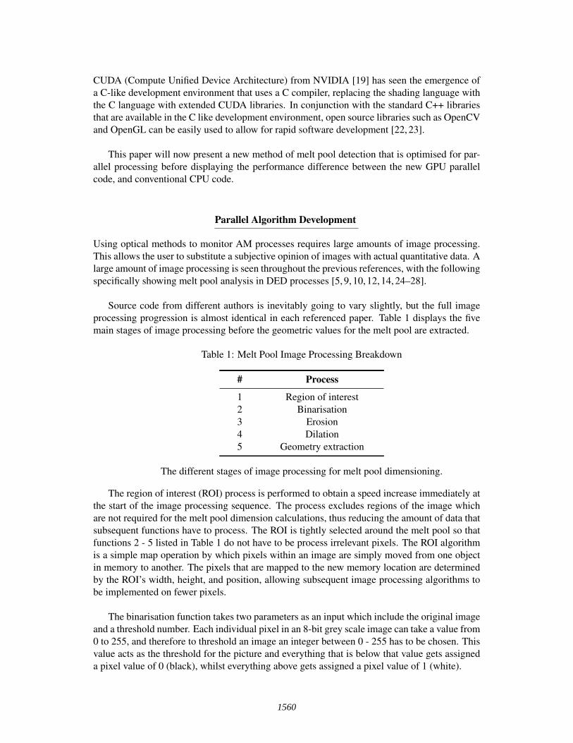
Source code from different authors is inevitably going to vary slightly, but the full imageprocessing progression is almost identical in each referenced paper. Table 1 displays the fivemain stages of image processing before the geometric values for the melt pool are extracted.

Table 1: Melt Pool Image Processing Breakdown

# Process

1 Region of interest2 Binarisation3 Erosion4 Dilation5 Geometry extraction

The different stages of image processing for melt pool dimensioning.

The region of interest (ROI) process is performed to obtain a speed increase immediately atthe start of the image processing sequence. The process excludes regions of the image whichare not required for the melt pool dimension calculations, thus reducing the amount of data thatsubsequent functions have to process. The ROI is tightly selected around the melt pool so thatfunctions 2 - 5 listed in Table 1 do not have to be process irrelevant pixels. The ROI algorithmis a simple map operation by which pixels within an image are simply moved from one objectin memory to another. The pixels that are mapped to the new memory location are determinedby the ROI’s width, height, and position, allowing subsequent image processing algorithms tobe implemented on fewer pixels.

The binarisation function takes two parameters as an input which include the original imageand a threshold number. Each individual pixel in an 8-bit grey scale image can take a value from0 to 255, and therefore to threshold an image an integer between 0 - 255 has to be chosen. Thisvalue acts as the threshold for the picture and everything that is below that value gets assigneda pixel value of 0 (black), whilst everything above gets assigned a pixel value of 1 (white).

1560

Erosion and dilation are very similar image processes with a slight difference. Both imageprocessing techniques take an input image as well as a kernel. The kernel is a shape, usually asquare, that has a single anchor point in the centre of it. The size of the kernel is a major char-acteristic of the technique that governs the output image. For each individual pixel, the kernel isplaced over the top with the processed pixel acting as the anchor point, and the kernel coveringthe surrounding pixels. Then either the local maximal (dilation process) or minimal (erosionprocess) pixel value that is within the kernel replaces the pixel at the anchor point. Erosion isprimarily carried out to reduce the amount of noise in the image, which in this process could becaused by light reflected off stray particles, followed by a dilation process to replace the pixelsthat have been previously eroded.

Once the ROI, binarisation, erosion and dilation processes have been carried out on theframe, the resulting image has a similar appearance to that displayed in figure 3. The imageshown is essentially a white ellipse surrounded by black pixels with its size representative ofthat of the melt pool. With this image, the process of melt pool dimensioning can be performed.

There have been two previously reported techniques for melt pool dimensioning. Originallya simple algorithm that detected the first white pixel moving from north, south, east, and westdirections was used, but this algorithm often produced dimensions that were larger than themelt pool if not all noise was eradicated through the erosion process [9]. This issue led to thesubsequent development of a moment technique that uses a Canny edge detection to create avector that stores pixel location of all the pixels that are at the circumference of the melt pool.This vector can then be used to calculate moments, which can subsequently be used to calculatecentre, orientation, and size of detected shapes. With these details, geometric shapes can besuperimposed onto the Canny edge image and be used to extract geometric characteristics ofthe melt pool [29].

Figure 3: Image of the melt pool after casting a ROI and performing binarisation, erosion anddilation image processing techniques.

The Canny edge technique is a five step process that first uses a Gaussian filter to smooththe image. The Gaussian filter is used as all edge detection results are easily influenced by noise

1561

within the image and acts to smooth the image for further image processing. Vertical, horizontaland diagonal edge detection operators are then implemented onto the image to determine thefirst derivative in both the horizontal and vertical directions. From these two first derivativesthe edge gradient and direction can be found. The edges detected by this point are blurred andso a non-maximum suppression process is carried out in order to thin the edges. This tech-nique suppresses all gradient values to zero, except the local maximal that is representative ofthe largest intensity value change. A double threshold is then implemented to eradicate weakedges that have been created due to noise and colour variation. High and low threshold valuesare determined by the original image and are used to categorise edges as either weak or strong.Finally edge tracking by hysteresis is carried out and all strong edges that were previously de-fined are determined as true edges. All weak edges are subjected to blob analysis, which is aprocess that checks the surrounding eight pixels of the edge pixel to determine whether theyare part of a strong edge or not. If one of these surrounding pixels is a pixel within a strongedge, it is determined that the weak edge is true and should be preserved. All remaining weakedges are believed to be caused by noise and/or colour variations, and are eradicated from thefinal Canny edge image. The following references use this technique and discuss it in moredetail [11, 12, 14, 29].

Although the moment technique described provides an adequate way of providing melt pooldimensions, the code to write this algorithm is linear and is computationally expensive. Runningthis algorithm through a CPU results in a low frame rate, and has resulted in many scientistsand engineers looking towards FPGA’s for code acceleration. This method of accelerating theimage processing however can be performed computationally by using a GPU with the follow-ing technique.

The company NVIDIA have built their GPU on what is known as the CUDA architecture.This has allowed the GPU to be able to perform both graphics rendering tasks and general pur-pose tasks. They have developed their own language in CUDA C which is essentially C, butwith a handful of extensions to allow for massively parallel programming on the graphics card.The technique works by creating a kernel, which is a relatively simple section of code that canbe launched on multiple microprocessors within the GPU in parallel. The launch configurationdefines the number of blocks in which the code will operate on. These blocks are simultane-ously executed by a microprocessing unit within the GPU. Threads are organised in blocks, andare a way of identifying the raw data that is passed into the kernel. A block contains an array ofthreads that can access data within a kernel. A grid contains and array of blocks that can eachbe assigned to a microprocessor to simultaneously run calculations.

Using this parallel technique the image pictured in figure 3 can be broken down into moremanageable data for melt pool dimensioning. The first kernel that is run in the newly developedalgorithm is a reduction kernel.

This technique is one of the fundamental techniques used in CUDA programming, and hasthe same outcome compared to individually adding up all of the values within a one dimensionalarray. This problem is inherently linear, as the full summation is dependent on the previoussummation of each individual index. Although this is true, the technique can be implementedin a parallel manner through a technique pictured in figure 4. This technique breaks down thesummation of elements into working sets as displayed. In the first working set, every otherelement (spacing of two) in the sequence is summed with its neighbouring elements (distance

1562

of one) to give intermediate summation values. In subsequent sets, the indexes of the elementsthat are being added to are doubled (spacing of four), and are summed with the integers fromelements with distance of two away (distance of two). In each iteration, the spacing betweenthe primary elements that are being added to doubles, with spacing starting at two. In eachiteration the distance between the secondary elements that are adding to the primary elementsdoubles, with the distance between them starting at one. This process can be done with an arrayof any length, with calculations continuing until distances and spacings fall outside the lengthof the array. Any calculation that requires an index that falls outside that of the original arrayis not performed. In both a linear and parallel summation of elements, the amount of workingcalculations required to perform a full reduction is then classed as N-1, where N is the sizeof the matrix being reduced. The difference between the two techniques lies with the workcomplexity (number of stages). A linear solution to the reduction problem will have N-1 stagesuntil a full calculation is complete. In a parallel solution, the work complexity is related to thesize of the matrix by log2N.

Figure 4: A schematic representation of the reduction technique to aid description [19].

This parallel reduction technique is for a singular dimensional array of elements, but can beimplemented on an entire image in parallel using the CUDA architecture. This is achieved byassigning a block to each individual row within an image and by assigning a singular thread ineach block to every pixel. This not only allows for a parallel implementation of the reductiontechnique described above, but also allows for the summation of each row simultaneously byassigning every row calculation to a different microprocessor (block). Figure 5 displays thekernel launch configurations with B01 - B10 corresponding to the individual blocks, and with’T’ corresponding to each individual thread in a 10 x 10 image. The summations of all thecolumns can be calculated using the same kernel, but with a transposed launch configuration tothat displayed in figure 5.

Once the kernel has been launched and the calculations are complete, the user is left withtwo single dimensional arrays that are summations of all of the rows and all the columns. Figure6 displays the summation of all of the column values and all of the row values for the imagedisplayed in figure 3. From this graph the user can see the edges of the melt pool representedby the breakouts from the X-axis, as well as being able to view the points of maximum widthrepresented by the Gaussian peaks. Although analysis of this distribution is useful in under-standing the melt pool, a further conversion of data is required to allow for a more accurate

1563

Figure 5: A schematic representation of the launch configuration for the summation of all rowsin a 10 x 10 pixel image.

extraction of melt pool dimensions from the frame. The reduction vector that was created usingthe previously mentioned technique is then subject to another common technique used in paral-lel programming called scan.

Figure 6: The distribution of row and column pixel summations as a function of pixel location.

The scan technique takes an input array and calculates the running sum of elements up to(exclusive), and sometimes including (inclusive), the given index. For this algorithm develop-ment the inclusive scan technique was used. Scan, like reduce, initially appears as a purelylinear problem, however there are techniques that can allow scan to be implemented in parallel.There are multiple ways in which scan can be implemented in parallel, but the method usedin this papers entails the Hills/Steele method displayed in figure 7 [30]. The method worksinitially by taking each element in the series (n), and adding the element n-1 to it. Any numberthat does not have a previous element with a distance of one, for example the number one inthe first index, is simply mapped to the same index in the next array. In the second stage thesame rule applies but the distance is doubled to two. Element n is summed with element n-2,whilst indexes that do not have two prior elements merely map to the next array. The distance

1564

between summing indexes keeps doubling until all elements within the array are mapped to thenew array and no more summations are required.

Figure 7: A schematic representation of the scan technique to aid description.

For the linear solution, the amount of working calculations that are needed to complete thealgorithm is N. The amount of stages needed to complete the algorithm is also N. For the par-allel solution, the amount of stages required for the completion of the scan technique is log2N.The amount of working calculations that are performed in this algorithm is equal to Nlog2N.The launch configurations for this method initiates a single block with N number of threads.

This scan technique is implemented on both the column and row reduction arrays to obtainaccumulative values as the array progresses. In doing so, this produces an array of numbersin which the centre and size of the melt pool can easily be extracted from in the third parallelstage. This technique alters the Gaussian distribution into a graph that represents a curve similarto y = x1/3. The scan arrays calculated for the melt pool in figure 3 are displayed in figure 8.

Figure 8: A scan function that shows the accumulated values of the Gaussian distribution ingraph 6.

1565

The last parallel technique implemented into the melt pool dimensioning is the extractionof the melt pools centre of mass, and the dimensions themselves. To perform this process, thecentre of the melt pool is calculated simply by halving the maximum values within the two scansequences, and iterating through each array to determine what the pixel location is for this value.

The upper and lower boundaries for the melt pool are also calculated by setting bound-ary thresholds that correspond with the melt pool dimensions. The lower threshold value iscalculated at 0.01% of the maximum value within the array, and the upper threshold value iscalculated as 99.99% of the maximum value within the array. These small deviations from ex-treme values (0% and 100%) allow the image to be able to achieve accurate results despite noiseadded to the image.

The iteration through the scan array has also been converted into a parallel kernel. A linearsolution would have to iterate through the array to find the index (pixel location) in which theupper, middle, and lower thresholds are located. Instead of passing the entire array though theCPU, whilst the data is on the GPU, a kernel can be used to check each individual array elementfor their values in parallel. This is done by creating three if statements within a kernel andlaunching it with a single block containing N number of threads.

In conjunction with the development of the new geometry extraction algorithm, a parallelimplementation of the ROI, binarisation, erosion and dilation functions have all been made toincrease total image processing speeds.

Results

A new algorithm has been developed that can be implemented on GPU units to perform meltpool measurements. To check the reliability and speed of this new algorithm, the algorithm hasbeen subjected to timing and has been compared to a moment-based melt pool dimensioningtechnique that is implemented on a CPU. Both algorithms have been implemented on a per-sonal laptop which contains an Intel Core i7-6820HK CPU clocked at 2.70GHz. This is a quadcore processor with 8 logical processors. The GPU that is used for the GPGPU acceleration isa NVIDIA GeForce GTX 980M. The full technical specifications for the components can befound within the following references [19, 31].

To distinguish the speed of the new algorithm a high resolution timer was used within thestandard C++ library. This clock has the highest precision of all the standard timers and has aresolution of 1 nanosecond on Visual Studio 2015 version 4.6.01586.

The high resolution timer was placed around all of the functions within the code separatelyto determine whether the GPU accelerated code could grant a performance boost on the originalCPU code. Multiple videos were run through the program to determine any major timing de-pendencies, but after initial testing, a video with 809 frames was chosen for the comparison run.Both the CPU and the GPU algorithm were run on the same video, and timings for individualframes were added together to provide an average execution time for each function across the809 frames. Table 2 displays the average execution times for the CPU functions, and the GPUaccelerated equivalent.

The table clearly shows an increase in speed of execution on all functions that are performed

1566

on the GPU. Using the GPU for code acceleration allowed for a performance speed increase ofover 60 times what the CPU could perform and has allowed for real time execution of melt poolimage processing techniques without the use of FPGAs.

Table 2: Execution Results

Task CPU Time(ms) CPU Time(ms) Performance Increase

Region of interest 472.7 6.1 78.0Binarisation 32.9 5.1 6.4

Erosion 517.6 5.5 94.2Dilation 500.9 4.9 102.1

Geometry extraction 1395.5 26.7 52.5Total time 2919.6 48.3 60.4

Time taken to execute individual functions on a CPU and GPU.

Whilst this technique has seen a drastic speed increase in process execution time, the GPUacceleration does come with a cost. To perform GPU calculations, memory needs to be allo-cated on the GPU and raw data has to be transferred from the CPU to the GPU. Fortunatelyfor the user, memory allocation only has to be performed once before the first frame, and thememory can be written over when processing subsequent frames. The time taken to allocatememory for the entire process is around 350 milliseconds. Whilst this is a drastically longertime than it takes to perform any of the actual image processing functions, the allocation ofmemory to the GPU can be performed at any time before image processing is carried out. Thismeans that this step in the technique can be integrated in the loading phase of the program andwill have no detrimental effect on individual frame processing speed.

The major bottleneck of this process lies within the copying of memory to and from theGPU. This was noticed early on in the development of the program, and the amount of infor-mation that is copied to and from the GPU was limited in the design. With each frame iteration,the original frame is copied from the CPU to the GPU, and after processing is completed, twoarrays containing melt pool information are returned. The returned array contain values for thetop, bottom, left and right extremes of the melt pool, as well as the centre location (x,y). Theoriginal frame that is copied across is a 1600 x 1200 resolution image with three separate chan-nels (5760000 bytes). The image processing data that is returned from the GPU to the CPU istwo integer arrays with lengths of 3 (24 bytes). The time taken to copy the image from the CPUto the GPU is around 850 microseconds. The time taken to copy the arrays from the GPU tothe CPU is around 150 microseconds. The time taken to copy memory to and from the GPU isaround 20 times that of the actual image processing time executed on the GPU. Nevertheless,the performance increase from using the GPU instead of the CPU is still around threefold.

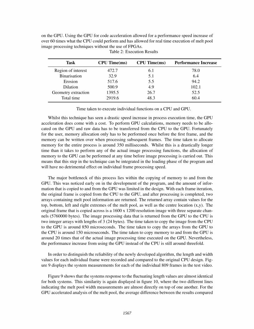
In order to distinguish the reliability of the newly developed algorithm, the length and widthvalues for each individual frame were recorded and compared to the original CPU design. Fig-ure 9 displays the system measurements for each of the individual 809 frames in the test video.

Figure 9 shows that the systems response to the fluctuating length values are almost identicalfor both systems. This similarity is again displayed in figure 10, where the two different linesindicating the melt pool width measurements are almost directly on top of one another. For theGPU accelerated analysis of the melt pool, the average difference between the results compared

1567

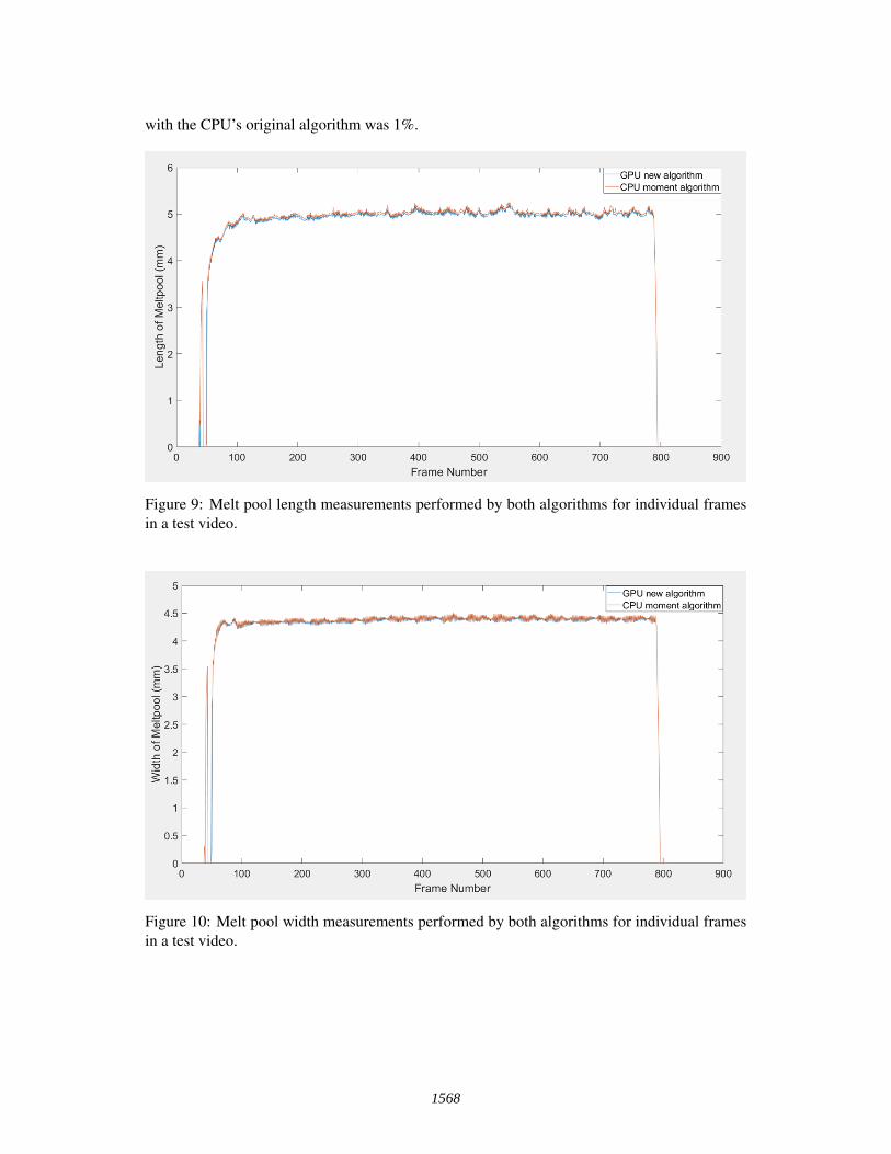
with the CPU’s original algorithm was 1%.

Figure 9: Melt pool length measurements performed by both algorithms for individual framesin a test video.

Figure 10: Melt pool width measurements performed by both algorithms for individual framesin a test video.

1568

Conclusion

The previously mentioned technique has allowed for the implementation of GPGPU program-ming in the field of AM for melt pool monitoring. The code that has been developed has allowedfor the accurate reading of melt pool dimensions utilising graphics card processing to enhancespeed.

The execution speed for each of the individual functions was drastically improved usingparallel GPGPU techniques, with the total execution time being over 60 times faster than thatof the CPU equivalent. This being said, a major bottleneck was found in the data transfer ratebetween the CPU and the GPU. This movement of data is required for each frame and costsaround 20 times as much as the actual code itself.

The code execution time including the data transfers from the GPU to the CPU is still nearlythree times faster using the GPGPU technique with no noticeable effects on the accuracy ofmeasurements. This has allowed for real time measurements of the melt pool in DED processesusing software techniques.

Whilst there are some limitations in the code run time, the technique developed can allowfor the further integration of advanced melt pool analysis techniques with very little cost to theexecution time. CPUs and FPGAs are linear processing techniques which are designed to haveas little latency as possible, whilst the parallel nature of GPGPU processing is optimised formaximum throughput. GPGPU techniques are best suited for computational heavy processingalgorithms that can be computed using parallel techniques, meaning that complex algorithmsare best suited for these applications. Adding further parallel image processing techniques tothe existing code will allow for a deeper understanding on the melt pool actions, whilst havingminimal effect on the programs execution time. The major drawback of using this technique isthe large data transfer of the original image from the CPU to the GPU, not the implementationsof the functions themselves.

References

[1] T. Wohlers and T. Gornet, “History of additive manufacturing Introduction of non-SLsystems Introduction of low-cost 3D printers,” Wohlers Report 2012, pp. 1–23, 2012.

[2] T. Wohlers and T. Caffery, Wohlers Report, 2015.

[3] T. G. Spears and S. A. Gold, “In-process sensing in selective laser melting (SLM) additivemanufacturing,” Integrating Materials and Manufacturing Innovation, vol. 5, no. 1, p. 2,2016. [Online]. Available: http://www.immijournal.com/content/5/1/2

[4] Mike Titsch, “3D Printer World,” 2016. [Online]. Available: http://www.3dprinterworld.com

[5] M. Asselin, E. Toyserkani, M. Iravani-Tabrizipour, and A. Khajepour, “Develop-ment of trinocular CCD-based optical detector for real-time monitoring of lasercladding,” Proceedings of the IEEE International Conference on Mechatronics & Au-tomation, Niagara Falls, Canada, no. July, pp. 1190–1196, 2005. [Online]. Available:http://ieeexplore.ieee.org/xpls/abs_all.jsp?arnumber=1626722

1569

[6] J. Kruth, P. Mercelis, J. V. Vaerenbergh, and T. Craeghs, “Feedback control of SelectiveLaser Melting,” pp. 1–7, 2007.

[7] S. Berumen, F. Bechmann, S. Lindner, J.-P. Kruth, and T. Craeghs, “Quality control oflaser- and powder bed-based Additive Manufacturing (AM) technologies,” Physics Proce-dia, vol. 5, pp. 617–622, 2010.

[8] T. Craeghs, F. Bechmann, S. Berumen, and J. P. Kruth, “Feedback control of LayerwiseLaser Melting using optical sensors,” Physics Procedia, vol. 5, no. PART 2, pp. 505–514,2010. [Online]. Available: http://dx.doi.org/10.1016/j.phpro.2010.08.078

[9] P. Colodrón, J. Fariña, J. J. Rodríguez-Andina, F. Vidal, J. L. Mato, and M. Á. Monteale-gre, “FPGA-based measurement of melt pool size in laser cladding systems,” Proceedings- ISIE 2011: 2011 IEEE International Symposium on Industrial Electronics, pp. 1503–1508, 2011.

[10] P. Colodrón, J. Fariña, J. J. Rodríguez-Andina, F. Vidal, and J. L. Mato, “PerformanceImprovement of a Laser Cladding System Through FPGA-based Control,” IECON Pro-ceedings (Industrial Electronics Conference), pp. 2814–2819, 2011.

[11] T. Craeghs, S. Clijsters, E. Yasa, and J.-P. Kruth, “Online quality control ofselective laser melting,” Solid Freeform Fabrication Proceedings, pp. 212–226, 2011.[Online]. Available: http://utwired.engr.utexas.edu/lff/symposium/proceedingsarchive/pubs/Manuscripts/2011/2011-17-Craeghs.pdf

[12] J. R. Araujo, J. J. Rodriguez-Andina, J. Farina, F. Vidal, J. L. Mato, and M. A.Montealegre, “FPGA-based laser cladding system with increased robustness to opticaldefects,” IECON 2012 - 38th Annual Conference on IEEE Industrial Electronics Society,pp. 4688–4693, 2012. [Online]. Available: http://ieeexplore.ieee.org/lpdocs/epic03/wrapper.htm?arnumber=6389491

[13] A. Heralic, A.-K. Christiansson, and B. Lennartson, “Height control of laser metal-wire deposition based on iterative learning control and 3D scanning,” Optics andLasers in Engineering, vol. 50, no. 9, pp. 1230–1241, 2012. [Online]. Available:http://linkinghub.elsevier.com/retrieve/pii/S0143816612001017

[14] J. Hofman, B. Pathiraj, J. van Dijk, D. de Lange, and J. Meijer, “A camerabased feedback control strategy for the laser cladding process,” Journal of MaterialsProcessing Technology, vol. 212, no. 11, pp. 2455–2462, 2012. [Online]. Available:http://dx.doi.org/10.1016/j.jmatprotec.2012.06.027

[15] Y. Chivel, “Optical in-process temperature monitoring of selective laser melting,” PhysicsProcedia, vol. 41, pp. 904–910, 2013. [Online]. Available: http://dx.doi.org/10.1016/j.phpro.2013.03.165

[16] S. Buls, S. Clijsters, and J.-P. Kruth, “Homogenizing the melt pool intensity distributionin the SLM process through system identification and feedback control,” Solid FreeformFabrication Symposium, pp. 6–11, 2014.

[17] V. Carl, “Monitoring System for the Quality Assessment in Additive Manufacturing,” 41StAnnual Review of Progress in Quantitative Nondestructive Evaluation, Vol 34, vol. 1650,pp. 171–176, 2015.

1570

[18] A. R. Nassar, J. S. Keist, E. W. Reutzel, and T. J. Spurgeon, “Intra-layerclosed-loop control of build plan during directed energy additive manufacturing ofTi-6Al-4V,” Additive Manufacturing, vol. 6, pp. 39–52, 2015. [Online]. Available:http://dx.doi.org/10.1016/j.addma.2015.03.005

[19] N. Website, “NVIDIA,” 2017. [Online]. Available: http://www.nvidia.co.uk/

[20] M. Galloy, “Michael Galloy Research,” 2016. [Online]. Available: http://michaelgalloy.com/2013/06/11/cpu-vs-gpu-performance.html#comment-798997

[21] Z. Yang, Y. Zhu, and Y. Pu, “Parallel Image Processing Based on CUDA,” pp. 198–201,2008.

[22] OpenCV, “OpenCV,” 2017. [Online]. Available: http://opencv.org/

[23] OpenGL, “OpenGL,” 2017. [Online]. Available: https://www.opengl.org/

[24] S. Barua, F. Liou, J. Newkirk, T. Sparks, J. N. Todd, D. Olivier, S. Borros, and G. Reyes,“Rapid Prototyping Journal Vision-based defect detection in laser metal deposition pro-cess Vision-based defect detection in laser metal deposition process,” Rapid PrototypingJournal Rapid Prototyping Journal, vol. 20, no. 1, pp. 77–85, 2014. [Online]. Available:http://dx.doi.org/10.1108/RPJ-04-2012-0036%5Cnhttp://dx.doi.org/10.1108/RPJ-01-2013-0012%5Cnhttp://dx.doi.org/10.1108/13552540510573365%5Cnhttp://dx.doi.org/10.1108/RPJ-01-2012-0002

[25] F. M. F. T. D. Grevey and a. B. Vannes, “Laser Cladding process and image processing,”Journal of laser in engineering, vol. 6, no. 33, pp. 161–187, 1997.

[26] D. Hu and R. Kovacevic, “Sensing, modeling and control for laser-based additive manu-facturing,” International Journal of Machine Tools and Manufacture, vol. 43, no. 1, pp.51–60, 2003.

[27] J. Mazumder, D. Dutta, N. Kikuchi, and A. Ghosh, “Closed loop direct metal deposition:Art to Part,” Optics and Lasers in Engineering, vol. 34, no. 4-6, pp. 397–414, 2000.

[28] F. Meriaudeau and F. Truchetet, “Control and optimization of the laser cladding processusing matrix cameras and image processing,” Journal of Laser Applications, vol. 8, no. 6,p. 317, 1996.

[29] OpenCV, “OpenCV Canny Edge Detector,” 2014. [Online]. Available: http://docs.opencv.org/2.4/doc/tutorials/imgproc/imgtrans/canny_detector/canny_detector.html

[30] W. D. Hillis and G. U. Y. L. Steele, “Data parallel algorithms,” vol. 29, no. 12, 1986.

[31] I. website, “Intel,” 2017. [Online]. Available: http://www.intel.co.uk/content/www/uk/en/products/processors/core/i7-processors/i7-6820hk.html?wapkw=6820hk

1571