meg 741 energy and variational methods in …bj/meg_741_f04/lectures/lecture 05.pdf5-1 meg 741...
TRANSCRIPT

5-1
MEG 741 Energy and Variational Methods in Mechanics I
Brendan J. O’Toole, Ph.D.Associate Professor of Mechanical Engineering
Howard R. Hughes College of EngineeringUniversity of Nevada Las Vegas
TBE B-122(702) 895 - [email protected]
Chapter 2: Principles of Virtual Work: Integral Form of the Basic Equations

5-2
Virtual Work and Variational Methods
Energy principles provide an alternative to Newtonian methodsas a means of deriving and solving governing equations.

5-3
Work & Energy• Applied forces, moments, and torques do work
on a structure, e.g., W=F.L
• This work changes the potential energy state of the internal forces– This is referred to as internal energy or strain energy
• The strain energy can be defined in terms of stresses & strains
• Applied Work (external) = Change of internal energy
direction in the force ofcomponent theis where , dsFs sdsFdW =
5-4
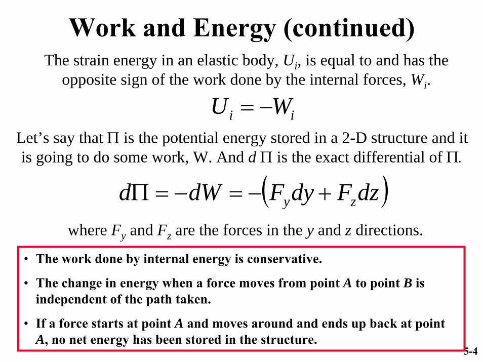
Work and Energy (continued)
ii WU −=
The strain energy in an elastic body, Ui, is equal to and has the opposite sign of the work done by the internal forces, Wi.
( )dzFdyFdWd zy +−=−=Π
Let’s say that Π is the potential energy stored in a 2-D structure and it is going to do some work, W. And d Π is the exact differential of Π.
where Fy and Fz are the forces in the y and z directions.
• The work done by internal energy is conservative.
• The change in energy when a force moves from point A to point B is independent of the path taken.
• If a force starts at point A and moves around and ends up back at point A, no net energy has been stored in the structure.

5-5
Work and Potential Energy of Internal ForcesExternal forces, N, are applied at the ends of the rod shown below.
What is the work done during the deformation of this bar?
NN
L
( )[ ]
AN
dxddxdu
x
xxxx
σ
εεεε
=
=−+=stress of in terms written becan force internal The
iselement aldifferenti theoflength in change The
First examine the work done by the internal forces, N, over the differential element of length, dx.
dx
N N
dx
N N
x1 2
xx dεε +xε
The net work over the differential element is N•u :
AdxddxAdworknet xxxx εσεσ ==

5-6
Internal Work due to Axial LoadThe internal work over the length of the bar is found by integrating the previous expression: NN
L
dx
N N
xxxi
xi
x
L
i
L
xxi
L
xxi
VVEW
LAEW
dxAEW
AdxdEW
AdxdW
x
x
εσε
ε
ε
εε
εσε
ε
212
21
221
2
0 21
0 0
0 0
−=−=
−=
−=
−=
−=
∫∫ ∫∫ ∫
Since σx = Eεx
If εx is constant over L
The capacity of the internal forces to do work is called strain energy, Ui. The strain energy is considered a positive quantity. The work done by the internal forces is negative:
xxxi
xxxi
VVEW
VVEU
εσε
εσε
212
21
212
21
−=−=
==ii WU −=

5-7
General LoadingThe internal work over the length of the bar is found by integrating the previous expression:
dVddd
dddW
Vyzyzxzxzxyxy
zzyyxxi yzxzxy
zyx
∫∫∫∫∫∫∫
⎥⎥
⎦
⎤
⎢⎢
⎣
⎡
++
+++= γγγ
εεε
γτγτγτ
εσεσεσ
000
000
∫∫∫∫
==
−=−=
VVi
VVi
dVdVU
dVdVW
or
Eεεσ
EεεσTT
TT
ε
ε
21
21
21
21
The strain energy density is defined as the strain energy per unit volume.
Eεεσ TT ε21
21 ==
=
o
io
UV
UU

5-8
Strain Energy Density and Complementary Strain Energy Density
xσ
oU
*oU
xε
Uo ≡ strain energy density
Uo ≡ complementary strain energy density*

5-9
Example 2.1: Find the Strain Energy in a Beam with an Internal Axial Force and Bending Moment
∫ ∫
∫
∫
⎥⎦
⎤⎢⎣
⎡++=
⎥⎦
⎤⎢⎣
⎡⎟⎠⎞
⎜⎝⎛ +⎟⎠⎞
⎜⎝⎛ +=
=+=
=
L
Ai
Vi
xxx
V xxi
dAdxI
zMAINMz
AN
EU
dVI
MzAN
IMz
AN
EU
EIMz
AN
dxU
0 2
22
2
2 2121
121
,
21
σεσ
εσ
∫∫
=
=
A
A
IdAz
zdA2
0
thatrecall
∫ ⎟⎟⎠
⎞⎜⎜⎝
⎛+=
L
i dxEI
MEANU
0
22
22The Strain Energy for Beam Problems:

5-10
In Some Cases, the Internal Work is not Simply Equal to a Potential Function
If the internal work depends on the loading history (and not just the end states) then it is not equal to a potential function.
Example: A slender bar has an applied axial stress and a temperature change x σx, ∆T
xσ
xεA B
C D
oε ( ) finalxε
xσ
xεA B
C D
( ) finalxεoε
Case I: Temperature Change Applied First
• ∆T applied with no constraint (stress free expansion from A to B)
• Applied Stresses cause εx between B and C
• Arrive at final stress and strain at D
Case II: Stress Applied First
• Applied Stresses cause εx between A and C
• ∆T applied under constant stress from C to D
• Arrive at same final stress and strain at D
The internal work is equal to the area under the stress strain curves. It is not the same in both cases.

5-11
Work of the Applied Forces (External Work)
x ΝConsider an axial bar with an applied force
Fe
Fu
e
u
e
uNW
kudu
kuW
Nku
duNW
F
F
21
21
that assume2
0
0
=
==
=
=
∫
∫

5-12
General Equations for External Work
∫∫
∫ ∫∫ ∫
+=
+=
ViV
Siie
V
u
iVS
u
iie
dVupdsupW
dVdupdsdupW
i
p
i
i
p
i
21
21
00
responselinear a with materialsFor

5-13
Some Fundamentals of Variational Calculus• A review of variational calculus is presented in Appendix I of
the textbook and summarized in the following pages.• Variational calculus involves finding extrema of functionals.
– A function is usually an expression involving independent variables; for example: f = f(x)
– A functional is a function of a function, or a function of dependent variables; for example, f = f(u,u´) , where u = g(x) and u´ = du/dx
• Variational calculus is used to derive energy concepts such as the principal of virtual work.
• The principle of virtual work requires an understanding of terms like – virtual displacements– virtual forces, and – virtual work

5-14
General Variational Calculus Problem
• Find the function u(x) such that
– In other words, find the u(x) that makes Π an extreme value• Necessary Conditions
– u = u(x) in the interval a ≤ x ≤ b– F is a known function (like strain energy density for example)– Usually require that u(x) be twice differentiable with respect
to x, (u´ and u″ exist)– And F be twice differentiable with respect to x, u, and u´
( ) ) (where stationary rendered is ,, dxdu
b
audxuuxF =′′=Π ∫

5-15
Virtual Displacements and the Variational Operator, δ
• Let u(x) be a family of neighboring paths of the extremizing path u(x)
uu ˆ,( )xu
( )xu
x
uδdu
dx
ax = bx =
)()()(ˆ xuxuxu δ+=Where u(x) is the extremizing path
and δu is a small variation away from the extremizing path. Note that:
endpoints at the 0ˆ
=−=
uuuu
δδ
• Notice that there is a big difference between du and δu• δ is called the variational operator and it has similar properties
as the differential operator d

5-16
Properties of the Variational Operator δ• The variational operator behaves like the differential operator in many ways.• For example, assume F = F(u,u´), where u´=du/dx, Then:
( )( )
( )
( ) ( ) 11
11
22
2121
2
1
212121
2121
FFnF
FFFFF
FF
FFFFFFFFFF
uuFu
uFF
nn δδδ
δδδ
δδδδδδ
δδδ
−=
+=⎟⎟
⎠
⎞⎜⎜⎝
⎛
+=+=+
′′∂
∂+
∂∂
=

5-17
Functionals and δ• A functional is an integral expression whose integrand(s) are
functions of dependent variables and their derivatives.
• The first variation of a functional can be calculated as follows
( ) ( ) dxdu
b
audxuuxFu =′′=Π ∫ where,,,
∫
∫∫
⎟⎠⎞
⎜⎝⎛ ′
′∂∂
+∂∂
=Π
==Π
b
a
b
a
b
a
dxuuFu
uF
FdxFdx
δδδ
δδδ
therefore

5-18
Extrema of Functionals• Suppose we wish to find the extemum of Π, where
• The necessary condition for the functional to have an extremum is that its first variation be zero, or
( ) ( ) ( ) ( ) ba
b
aubuuaudxuuxFu ==′=Π ∫ , ,,,
( ) 0
0
0
=⎟⎠⎞
⎜⎝⎛
′∂∂
+∂∂
=Π
=⎟⎠⎞
⎜⎝⎛ ′
′∂∂
+∂∂
=Π
=Π
∫
∫b
a
b
a
dxdx
uduFu
uF
dxuuFu
uF
δδδ
δδδ
δ

5-19
Extrema of Functionals• Use integration by parts to evaluate the second term in the
previous integral. The general procedure for integration by parts:
[ ]( )
( )
0
becomes 0
then, , , Define
=⎥⎦⎤
⎢⎣⎡
′∂∂
+⎥⎦
⎤⎢⎣
⎡⎟⎠⎞
⎜⎝⎛
′∂∂
−∂∂
=⎟⎠⎞
⎜⎝⎛
′∂∂
+∂∂
=∴==
−=
∫
∫
∫∫′∂
∂
b
a
b
a
b
a
dxud
uF
b
a
ba
b
a
uuFudx
uF
dxd
uF
dxdx
uduFu
uF
utdts
tdsstsdt
δδ
δδ
δδ

5-20
0=⎥⎦⎤
⎢⎣⎡
′∂∂
+⎥⎦
⎤⎢⎣
⎡⎟⎠⎞
⎜⎝⎛
′∂∂
−∂∂
∫b
a
b
au
uFudx
uF
dxd
uF δδ
Extrema of Functionals (continued)
• This equation can be simplified– The variation of u, (δu), at points a and b must be zero since u is
specified at those points; therefore:
bxauF
dxd
uF
u
udxuF
dxd
uF
uuF
b
a
b
a
<<=⎥⎦
⎤⎢⎣
⎡⎟⎠⎞
⎜⎝⎛
′∂∂
−∂∂
=⎥⎦
⎤⎢⎣
⎡⎟⎠⎞
⎜⎝⎛
′∂∂
−∂∂
=⎥⎦⎤
⎢⎣⎡
′∂∂
∫
,0
then value,zero)-(nonarbitrary an is if and
0
leaving ,0
δ
δ
δEuler Lagrange
EquationThis is a necessary
condition for a function u(x) to extremize the functional Π.

5-21
Example: Find the Path of Minimum Length Between Points 1 and 2
22 dydxds +=y
x
dy
dx
ax = bx =
ds
1
2
( )
dxy
dx
dydx
dydxds
dxdy
dxdx
dxdx
∫∫∫
∫∫
′+=Π
+=Π
+=Π
+==Π
2
1
2
2
1
2
1
22
2
1
222
1
1
2
2
2
2
21 yF ′+=In this case:

5-22
Minimum Path Example (Continued)
Apply the Euler Lagrange Equation:
0=⎟⎟⎠
⎞⎜⎜⎝
⎛′∂
∂−
∂∂
=⎟⎠⎞
⎜⎝⎛
′∂∂
−∂∂
yF
dxd
yF
uF
dxd
uFLet u = y for this problem:
( ) ( )
01
0
:BecomesEquation LagrangeEuler The1
2121
0
2
2
2 21
=⎟⎟
⎠
⎞
⎜⎜
⎝
⎛
′+
′−
′+
′=
′∂∂
′′+=′∂
∂
=∂∂
−
yy
dxd
yy
yF
yyyF
yF
),(1 2
yyFFyF′=
′+=

5-23
Minimum Path Example (Completed)
Solve the Euler Lagrange Equation:
( )
BAxyAy
AC
Cy
Cyy
Cyy
Cy
yy
ydxd
+==′
=−
=′
′+=′
′+=′
=′+
′∴=
⎟⎟
⎠
⎞
⎜⎜
⎝
⎛
′+
′
2
2
222
2
22
1
1
1
1 ,0
1
Apply boundary conditions at points 1 and 2 to find the
unknown constants A and B.

5-24
Next Class
• Discuss some Problems from HW 1• Discuss Semester Projects• Define Virtual Work Using Variational Calculus