Computer Physics Communications 181 (2010) 687–702

Contents lists available at ScienceDirect

Computer Physics Communications

www.elsevier.com/locate/cpc

Meep: A flexible free-software package for electromagnetic simulations by theFDTD method ✩

Ardavan F. Oskooi a,c,∗, David Roundy b, Mihai Ibanescu a,c,d, Peter Bermel c, J.D. Joannopoulos a,c,d,Steven G. Johnson a,c,e,∗∗a Center for Materials Science & Engineering, Massachusetts Institute of Technology, Cambridge, MA 02139, United Statesb Department of Physics, Oregon State University, Corvallis, OR 97331, United Statesc Research Laboratory of Electronics, Massachusetts Institute of Technology, Cambridge, MA 02139, United Statesd Department of Physics, Massachusetts Institute of Technology, Cambridge, MA 02139, United Statese Department of Mathematics, Massachusetts Institute of Technology, Cambridge, MA 02139, United States

a r t i c l e i n f o a b s t r a c t

Article history:Received 2 October 2009Received in revised form 13 November 2009Accepted 17 November 2009Available online 20 November 2009

Keywords:Computational electromagnetismFDTDMaxwell solver

This paper describes Meep, a popular free implementation of the finite-difference time-domain (FDTD)method for simulating electromagnetism. In particular, we focus on aspects of implementing a full-fea-tured FDTD package that go beyond standard textbook descriptions of the algorithm, or ways in whichMeep differs from typical FDTD implementations. These include pervasive interpolation and accuratemodeling of subpixel features, advanced signal processing, support for nonlinear materials via Padé ap-proximants, and flexible scripting capabilities.

Program summary

Program title: MeepCatalogue identifier: AEFU_v1_0Program summary URL:: http://cpc.cs.qub.ac.uk/summaries/AEFU_v1_0.htmlProgram obtainable from: CPC Program Library, Queen’s University, Belfast, N. IrelandLicensing provisions: GNU GPLNo. of lines in distributed program, including test data, etc.: 151 821No. of bytes in distributed program, including test data, etc.: 1 925 774Distribution format: tar.gzProgramming language: C++Computer: Any computer with a Unix-like system and a C++ compiler; optionally exploits additional freesoftware packages: GNU Guile [1], libctl interface library [2], HDF5 [3], MPI message-passing interface [4],and Harminv filter-diagonalization [5]. Developed on 2.8 GHz Intel Core 2 Duo.Operating system: Any Unix-like system; developed under Debian GNU/Linux 5.0.2.RAM: Problem dependent (roughly 100 bytes per pixel/voxel)Classification: 10External routines: Optionally exploits additional free software packages: GNU Guile [1], libctl interfacelibrary [2], HDF5 [3], MPI message-passing interface [4], and Harminv filter-diagonalization [5] (whichrequires LAPACK and BLAS linear-algebra software [6]).Nature of problem: Classical electrodynamicsSolution method: Finite-difference time-domain (FDTD) methodRunning time: Problem dependent (typically about 10 ns per pixel per timestep)References:[1] GNU Guile, http://www.gnu.org/software/guile[2] Libctl, http://ab-initio.mit.edu/libctl[3] M. Folk, R.E. McGrath, N. Yeager, HDF: An update and future directions, in: Proc. 1999 Geoscience and

Remote Sensing Symposium (IGARSS), Hamburg, Germany, vol. 1, IEEE Press, 1999, pp. 273–275.

✩ This paper and its associated computer program are available via the Computer Physics Communications homepage on ScienceDirect (http://www.sciencedirect.com/science/journal/00104655).

* Corresponding author at: Center for Materials Science & Engineering, Massachusetts Institute of Technology, Cambridge, MA 02139, United States.

** Principal corresponding author.E-mail addresses: ardavan@mit.edu (A.F. Oskooi), roundyd@physics.oregonstate.edu (D. Roundy), michel@alum.mit.edu (M. Ibanescu), bermel@mit.edu (P. Bermel),

joannop@mit.edu (J.D. Joannopoulos), stevenj@math.mit.edu (S.G. Johnson).

0010-4655/$ – see front matter © 2009 Elsevier B.V. All rights reserved.doi:10.1016/j.cpc.2009.11.008

688 A.F. Oskooi et al. / Computer Physics Communications 181 (2010) 687–702

[4] T.M. Forum, MPI: A Message Passing Interface, in: Supercomputing 93, Portland, OR, 1993, pp. 878–883.

[5] Harminv, http://ab-initio.mit.edu/harminv.[6] LAPACK, http://www.netlib.org/lapack/lug.

© 2009 Elsevier B.V. All rights reserved.

1. Introduction

One of the most common computational tools in classicalelectromagnetism is the finite-difference time-domain (FDTD) al-gorithm, which divides space and time into a regular grid andsimulates the time evolution of Maxwell’s equations [1–5]. Thispaper describes our free, open-source implementation of theFDTD algorithm: Meep (an acronym for MIT Electromagnetic Equa-tion Propagation), available online at http://ab-initio.mit.edu/meep.Meep is full-featured, including, for example: arbitrary anisotropic,nonlinear, and dispersive electric and magnetic media; a vari-ety of boundary conditions including symmetries and perfectlymatched layers (PML); distributed-memory parallelism; Cartesian(1d/2d/3d) and cylindrical coordinates; and flexible output andfield computations. It also includes some unusual features, suchas advanced signal processing to analyze resonant modes, accuratesubpixel averaging, a frequency-domain solver that exploits thetime-domain code, complete scriptability, and integrated optimiza-tion facilities. Here, rather than review the well-known FDTD algo-rithm itself (which is thoroughly covered elsewhere), we focus onthe particular design decisions that went into the development ofMeep whose motivation may not be apparent from textbook FDTDdescriptions, the tension between abstraction and performance inFDTD implementations, and the unique or unusual features of oursoftware.

Why implement yet another FDTD program? Literally dozensof commercial FDTD software packages are available for purchase,but the needs of research often demand the flexibility providedby access to the source code (and relaxed licensing constraints tospeed porting to new clusters and supercomputers). Our interac-tions with other photonics researchers suggest that many groupsend up developing their own FDTD code to serve their needs (ourown groups have used at least three distinct in-house FDTD im-plementations over the past 15 years), a duplication of effort thatseems wasteful. Most of these are not released to the public, andthe handful of other free-software FDTD programs that could bedownloaded when Meep was first released in 2006 were not nearlyfull-featured enough for our purposes. Since then, Meep has beencited in over 100 journal publications and has been downloadedover 10,000 times, reaffirming the demand for such a package.

FDTD algorithms are, of course, only one of many numeri-cal tools that have been developed in computational electromag-netism, and may perhaps seem primitive in light of other sophis-ticated techniques, such as finite-element methods (FEMs) withhigh-order accuracy and/or adaptive unstructured meshes [6–8],or even radically different approaches such as boundary-elementmethods (BEMs) that discretize only interfaces between homoge-neous materials rather than volumes [9–12]. Each tool, of course,has its strengths and weaknesses, and we do not believe that anysingle one is a panacea. The nonuniform unstructured grids ofFEMs, for example, have compelling advantages for metallic struc-tures where micrometer wavelengths may be paired with nanome-ter skin depths. On the other hand, this flexibility comes at a priceof substantial software complexity, which may not be worthwhilefor dielectric devices at infrared wavelengths (such as in integratedoptics or fibers) where the refractive index (and hence the typicalresolution required) varies by less than a factor of four betweenmaterials, while small features such as surface roughness can be

accurately handled by perturbative techniques [13]. BEMs, basedon integral-equation formulations of electromagnetism, are espe-cially powerful for scattering problems involving small objects ina large volume, since the volume need not be discretized and noartificial “absorbing boundaries” are needed. On the other hand,BEMs have a number of limitations: they may still require artificialabsorbers for interfaces extending to infinity (such as input/outputwaveguides) [14]; any change to the Green’s function (such as in-troduction of anisotropic materials, imposition of periodic or sym-metry boundary conditions, or a switch from three to two dimen-sions) requires re-implementation of large portions of the software(e.g. singular panel integrations and fast solvers) rather than purelylocal changes as in FDTD or FEM; continuously varying (as op-posed to piecewise-constant) materials are inefficient; and solutionin the time domain (rather than frequency domain, which is inad-equate for nonlinear or active systems in which frequency is notconserved) with BEM requires an expensive solver that is nonlocalin time as well as in space [11]. And then, of course, there are spe-cialized tools that solve only a particular type of electromagneticproblem, such as our own MPB software that only computes eigen-modes (e.g. waveguide modes) [15], which are powerful and robustwithin their domain but are not a substitute for a general-purposeMaxwell simulation. FDTD has the advantages of simplicity, gener-ality, and robustness: it is straightforward to implement the fulltime-dependent Maxwell equations for nearly arbitrary materi-als (including nonlinear, anisotropic, dispersive, and time-varyingmaterials) and a wide variety of boundary conditions, one canquickly experiment with new physics coupled to Maxwell’s equa-tions (such as populations of excited atoms for lasing [16–20]), andthe algorithm is easily parallelized to run on clusters or supercom-puters. This simplicity is especially attractive to researchers whoseprimary concern is investigating new interactions of physical pro-cesses, and for whom programmer time and the training of newstudents is far more expensive than computer time.

The starting point for any FDTD solver is the time-derivativeparts of Maxwell’s equations, which in their simplest form can bewritten:

∂B

∂t= −∇ × E − JB , (1)

∂D

∂t= +∇ × H − J, (2)

where (respectively) E and H are the macroscopic electric andmagnetic fields, D and B are the electric displacement and mag-netic induction fields [21], J is the electric-charge current den-sity, and JB is a fictitious magnetic-charge current density (some-times convenient in calculations, e.g. for magnetic-dipole sources).In time-domain calculations, one typically solves the initial-valueproblem where the fields and currents are zero for t < 0, andthen nonzero values evolve in response to some currents J(x, t)and/or JB(x, t). (In contrast, a frequency-domain solver assumes atime dependence of e−iωt for all currents and fields, and solves theresulting linear equations for the steady-state response or eigen-modes [22, Appendix D].) We prefer to use dimensionless unitsε0 = μ0 = c = 1. From our perspective, this choice emphasizesboth the scale invariance of Maxwell’s equations [22, Chapter 2]and also the fact that the most meaningful quantities to calcu-late are almost always dimensionless ratios (such as scattered

A.F. Oskooi et al. / Computer Physics Communications 181 (2010) 687–702 689

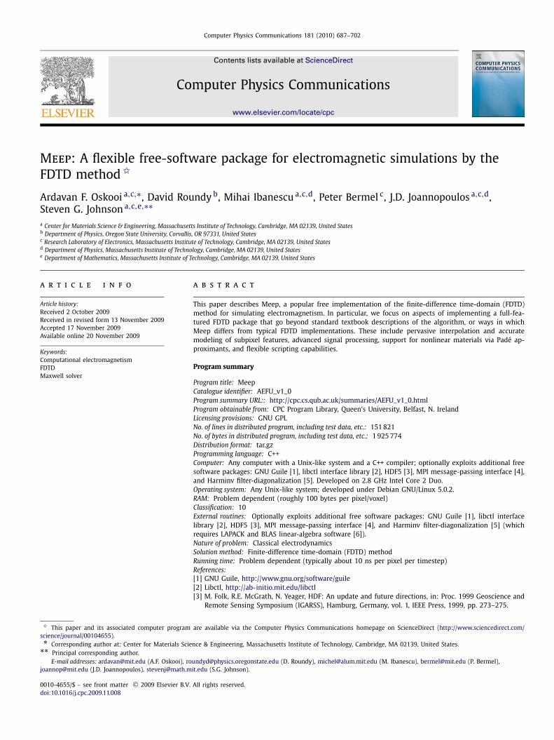
Fig. 1. The computational cell is divided into chunks (left) that have a one-pixel overlap (gray regions). Each chunk (right) represents a portion of the Yee grid, partitionedinto owned points (chunk interior) and not-owned points (gray regions around the chunk edges) that are determined from other chunks and/or via boundary conditions.Every point in the interior of the computational cell is owned by exactly one chunk, the chunk responsible for timestepping that point.

power over incident power, or wavelength over some character-istic lengthscale). The user can pick any desired unit of distancea (either an SI unit such as a = 1 μm or some typical length-scale of a given problem), and all distances are given in unitsof a, all times in units of a/c, and all frequencies in units of c/a.In a linear dispersionless medium, the constituent relations areD = εE and B = μH, where ε and μ are the relative permittivityand permeability (possibly tensors); the case of nonlinear and/ordispersive media (including conductivities) is discussed further inSection 4.

The remaining paper is organized as follows. In Section 2, wediscuss the discretization and coordinate system; in addition tothe standard Yee discretization [1], this raises the question of howexactly the grid is described and divided into “chunks” for par-allelization, PML, and other purposes. Section 3 describes a cen-tral principle of Meep’s design, pervasive interpolation providing (asmuch as possible) the illusion of continuity in the specification ofsources, materials, outputs, and so on. This led to the develop-ment of several techniques unique to Meep, such as a scheme forsubpixel material averaging designed to eliminate the first-ordererror usually associated with averaging techniques or stairstep-ping of interfaces. In Section 4, we describe and motivate ourtechniques for implementing nonlinear and dispersive materials,including a slightly unusual method to implement nonlinear ma-terials using a Padé approximant that eliminates the need to solvecubic equations for every pixel. Section 5 describes how typicalcomputations are performed in Meep, such as memory-efficienttransmission spectra or sophisticated analysis of resonant modesvia harmonic inversion. This section also describes how we haveadapted the time-domain code, almost without modification, tosolve frequency-domain problems with much faster convergenceto the steady-state response than merely time-stepping. The userinterface of Meep is discussed in Section 6, explaining the consid-erations that led us to a scripting interface (rather than a GUI orCAD interface). Section 7 describes some of the tradeoffs betweenperformance and generality in this type of code and the specificcompromises chosen in Meep. Finally, we make some concludingremarks in Section 8.

2. Grids and boundary conditions

The starting point for the FDTD algorithm is the discretizationof space and time into a grid. In particular, Meep uses the standardYee grid discretization which staggers the electric and magnetic

fields in time and in space, with each field component sampled atdifferent spatial locations offset by half a pixel, allowing the timeand space derivatives to be formulated as center-difference approx-imations [23]. This much is common to nearly every FDTD im-plementation and is described in detail elsewhere [1]. In order toparallelize Meep, efficiently support simulations with symmetries,and to efficiently store auxiliary fields only in certain regions (forPML absorbing layers), Meep further divides the grid into chunksthat are joined together into an arbitrary topology via boundaryconditions. (In the future, different chunks may have different res-olutions to implement a nonuniform grid [24–27].) Furthermore,we distinguish two coordinate systems: one consisting of integercoordinates on the Yee grid, and one of continuous coordinates in“physical” space that are interpolated as necessary onto the grid(see Section 3). This section describes those concepts as they areimplemented in Meep, as they form a foundation for the remain-ing sections and the overall design of the Meep software.

2.1. Coordinates and grids

The two spatial coordinate systems in Meep are described bythe vec, a continuous vector in R

d (in d dimensions), and theivec, an integer-valued vector in Z

d describing locations on theYee grid. If n is an ivec, the corresponding vec is given by0.5�xn, where �x is the spatial resolution (the same along x, y,and z)—that is, the integer coordinates in an ivec correspondto half -pixels, as shown in the right panel of Fig. 1. This is torepresent locations on the spatial Yee grid, which offsets differ-ent field components in space by half a pixel as shown (in 2d)in the right panel of Fig. 1. In 3d, the Ex and Dx componentsare sampled at ivecs (2� + 1,2m,2n), E y and D y are sampledat ivecs (2�,2m + 1,2n), and so on; Hx and Bx are sampledat ivecs (2�,2m + 1,2n + 1), H y and B y are sampled at ivecs(2� + 1,2m,2n + 1), and so on. In addition to these grids for thedifferent field components, we also occasionally refer to the cen-tered grid, at odd ivecs (2� + 1,2m + 1,2n + 1) corresponding tothe “center” of each pixel. (The origin of the coordinate systems isan arbitrary ivec that can be set by the user, but is typically thecenter of the computational volume.) The philosophy of Meep, asdescribed in Section 3, is that as much as possible the user shouldbe concerned only with continuous physical coordinates (vecs),and the interpolation/discretization onto ivecs occurs internallyas transparently as possible.

690 A.F. Oskooi et al. / Computer Physics Communications 181 (2010) 687–702

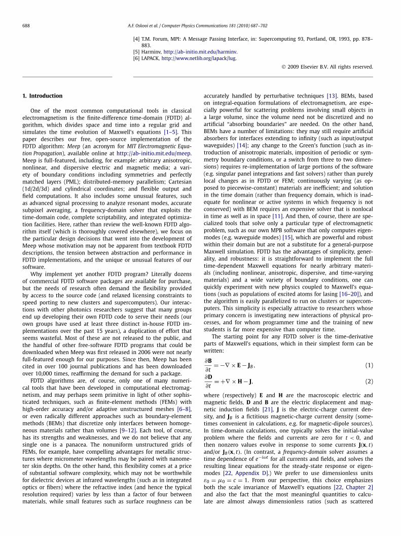
Fig. 2. Meep can exploit mirror and rotational symmetries, such as the 180-degree (C2) rotational symmetry of the S-shaped structure in this schematic example. AlthoughMeep maintains the illusion that the entire structure is stored and simulated, internally only half of the structure is stored (as shown at right), and the other half is inferredby rotation. The rotation gives a boundary condition for the not-owned grid points along the dashed line.

2.2. Grid chunks and owned points

An FDTD simulation must occur within a finite volume of space,the computational cell, terminated with some boundary conditionsand possibly by absorbing PML regions as described below. This(rectilinear) computational cell, however, is further subdivided intoconvex rectilinear chunks. On a parallel computer, for example, dif-ferent chunks may be stored at different processors. In order tosimplify the calculations for each chunk, we employ the commontechnique of padding each chunk with extra “boundary” pixels thatstore the boundary values [28] (shown as gray regions in Fig. 1)—this means that the chunks are overlapping in the interior of thecomputational cell, where the overlaps require communication tosynchronize the values.

More precisely, the grid points in each chunk are partitionedinto owned and not-owned points. The not-owned points are deter-mined by communication with other chunks and/or by boundaryconditions. The owned points are time-stepped within the chunk,independently of the other chunks (and possibly in parallel), andevery grid point inside the computational cell is owned by exactly onechunk.

The question then arises: how do we decide which pointswithin the chunk are owned? In order for a grid point to beowned, the chunk must contain all the information necessary fortimestepping that point (once the not-owned points have beencommunicated). For example, for a D y point (2�,2m + 1,2n) tobe owned, the Hz points at (2� ± 1,2m + 1,2n) must both be inthe chunk in order to compute ∇ × H for timestepping D at thatpoint. This means that the D y points along the left (minimum-x)edge of the chunk (as shown in the right panel of Fig. 1) cannotbe owned: there is no Hz point to the left of it. An additional de-pendency is imposed by the case of anisotropic media: if there isan εxy coupling Ex to D y , then updating Ex at (2� + 1,2m,2n) re-quires the four D y values at (2�+ 1 ± 1,2m ± 1,2n) (these are thesurrounding D y values, as seen in the right panel of Fig. 1). Thismeans that the Ex (and Dx) points along the right (maximum-x)edge of the chunk (as shown in the right panel of Fig. 1) cannotbe owned either: there is no D y point to the right of it. Similarlyfor ∇ × D and anisotropic μ.

All of these considerations result in the shaded-gray region ofFig. 1 (right) being not-owned. That is, if the chunk intersects k +1pixels along a given direction starting at an ivec coordinate of 0(e.g. k = 5 in Fig. 1), the endpoint ivec coordinates 0 and 2k + 1are not-owned and the interior coordinates from 1 to 2k (inclusive)are owned.

2.3. Boundary conditions and symmetries

All of the not-owned points in a chunk must be determinedby boundary conditions of some sort. The simplest boundary con-ditions are when the not-owned points are owned by some otherchunk, in which case the values are simply copied from that chunk

(possibly requiring communication on a multiprocessor system)each time they are updated. In order to minimize communicationsoverhead, all communications between two chunks are batchedinto a single message (by copying the relevant not-owned pointsto/from a contiguous buffer) rather than sending one message perpoint to be copied.

At the edges of the computational cell, some user-selectedboundary condition must be imposed. For example, one canuse perfect electric or magnetic conductors where the relevantelectric/magnetic-field components are set to zero at the bound-aries. One can also use Bloch-periodic boundary conditions, wherethe fields on one side of the computational cell are copied fromthe other side of the computational cell, optionally multiplied bya complex phase factor eikiΛi where ki is the propagation constantin the ith direction, and Λi is the length of the computational cellin the same direction. Meep does not implement any absorbingboundary conditions—absorbing boundaries are, instead, handledby an artificial material, perfectly matched layers (PML), placedadjacent to the boundaries [1].

Bloch-periodic boundary conditions are useful in periodic sys-tems [22], but this is only one example of a useful symmetry thatmay be exploited via boundary conditions. One may also have mir-ror and rotational symmetries. For example, if the materials andthe field sources have a mirror symmetry, one can cut the com-putational costs in two by storing chunks only in half the com-putational cell and applying mirror boundary conditions to obtainthe not-owned pixels adjacent to the mirror plane. As a more un-usual example, consider an S-shaped structure as in Fig. 2, whichhas no mirror symmetry but is symmetric under 180-degree rota-tion, called C2 symmetry [29]. Meep can exploit this case as well(assuming the current sources have the same symmetry), storingonly half of the computational cell as in Fig. 2 and inferring thenot-owned values along the dashed line by a 180-degree rotation.(In the simple case where the stored region is a single chunk, thismeans that the not-owned points are determined by owned pointsin the same chunk, requiring copies, possibly with sign flips.) De-pending on the sources, of course, the fields can be even or oddunder mirror flips or C2 rotations [22], so the user can specify anadditional sign flip for the transformation of the vector fields (andpseudovector H and B fields, which incur an additional sign flipunder mirror reflections [21,22]). Meep also supports four-fold ro-tation symmetry (C4), where the field can be multiplied by factorsof 1, i, −1, or −i under each 90-degree rotation [29]. (Other ro-tations, such as three-fold or six-fold, are not supported becausethey do not preserve the Cartesian Yee grid.) In 2d, the xy-planeis itself a mirror plane (unless in the presence of anisotropic ma-terials) and the symmetry decouples TE modes (with fields Ex , E y ,and Hz) from TM modes (Hx , H y , and Ez) [22]; in this case Meeponly allocates those fields for which the corresponding sources arepresent.

A central principle of Meep is that symmetry optimizations betransparent to the user once the desired symmetries are speci-

A.F. Oskooi et al. / Computer Physics Communications 181 (2010) 687–702 691

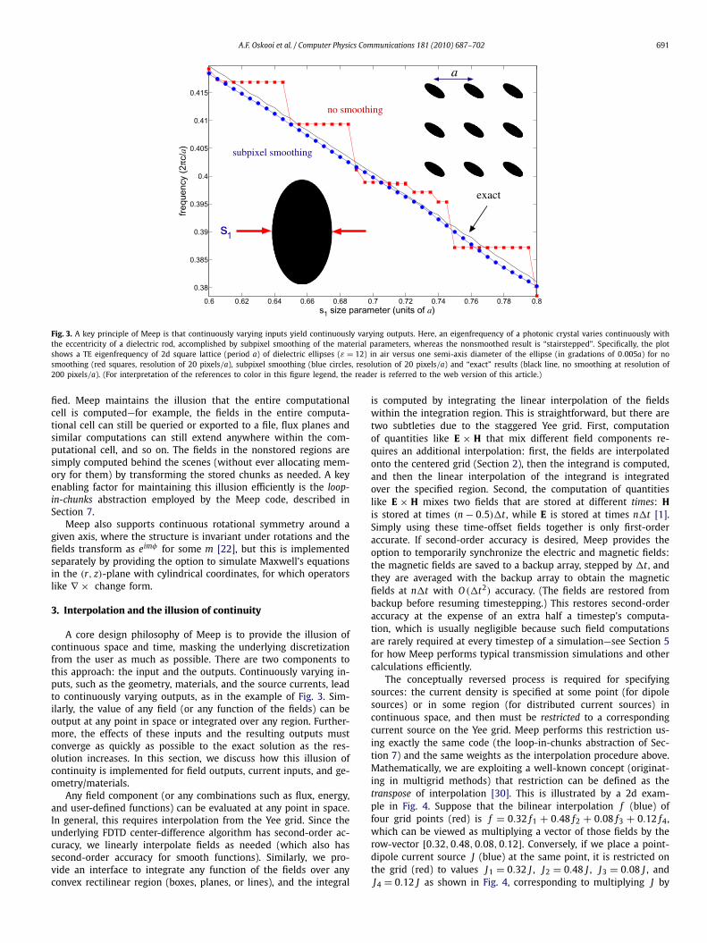
Fig. 3. A key principle of Meep is that continuously varying inputs yield continuously varying outputs. Here, an eigenfrequency of a photonic crystal varies continuously withthe eccentricity of a dielectric rod, accomplished by subpixel smoothing of the material parameters, whereas the nonsmoothed result is “stairstepped”. Specifically, the plotshows a TE eigenfrequency of 2d square lattice (period a) of dielectric ellipses (ε = 12) in air versus one semi-axis diameter of the ellipse (in gradations of 0.005a) for nosmoothing (red squares, resolution of 20 pixels/a), subpixel smoothing (blue circles, resolution of 20 pixels/a) and “exact” results (black line, no smoothing at resolution of200 pixels/a). (For interpretation of the references to color in this figure legend, the reader is referred to the web version of this article.)

fied. Meep maintains the illusion that the entire computationalcell is computed—for example, the fields in the entire computa-tional cell can still be queried or exported to a file, flux planes andsimilar computations can still extend anywhere within the com-putational cell, and so on. The fields in the nonstored regions aresimply computed behind the scenes (without ever allocating mem-ory for them) by transforming the stored chunks as needed. A keyenabling factor for maintaining this illusion efficiently is the loop-in-chunks abstraction employed by the Meep code, described inSection 7.

Meep also supports continuous rotational symmetry around agiven axis, where the structure is invariant under rotations and thefields transform as eimφ for some m [22], but this is implementedseparately by providing the option to simulate Maxwell’s equationsin the (r, z)-plane with cylindrical coordinates, for which operatorslike ∇ × change form.

3. Interpolation and the illusion of continuity

A core design philosophy of Meep is to provide the illusion ofcontinuous space and time, masking the underlying discretizationfrom the user as much as possible. There are two components tothis approach: the input and the outputs. Continuously varying in-puts, such as the geometry, materials, and the source currents, leadto continuously varying outputs, as in the example of Fig. 3. Sim-ilarly, the value of any field (or any function of the fields) can beoutput at any point in space or integrated over any region. Further-more, the effects of these inputs and the resulting outputs mustconverge as quickly as possible to the exact solution as the res-olution increases. In this section, we discuss how this illusion ofcontinuity is implemented for field outputs, current inputs, and ge-ometry/materials.

Any field component (or any combinations such as flux, energy,and user-defined functions) can be evaluated at any point in space.In general, this requires interpolation from the Yee grid. Since theunderlying FDTD center-difference algorithm has second-order ac-curacy, we linearly interpolate fields as needed (which also hassecond-order accuracy for smooth functions). Similarly, we pro-vide an interface to integrate any function of the fields over anyconvex rectilinear region (boxes, planes, or lines), and the integral

is computed by integrating the linear interpolation of the fieldswithin the integration region. This is straightforward, but there aretwo subtleties due to the staggered Yee grid. First, computationof quantities like E × H that mix different field components re-quires an additional interpolation: first, the fields are interpolatedonto the centered grid (Section 2), then the integrand is computed,and then the linear interpolation of the integrand is integratedover the specified region. Second, the computation of quantitieslike E × H mixes two fields that are stored at different times: His stored at times (n − 0.5)�t , while E is stored at times n�t [1].Simply using these time-offset fields together is only first-orderaccurate. If second-order accuracy is desired, Meep provides theoption to temporarily synchronize the electric and magnetic fields:the magnetic fields are saved to a backup array, stepped by �t , andthey are averaged with the backup array to obtain the magneticfields at n�t with O (�t2) accuracy. (The fields are restored frombackup before resuming timestepping.) This restores second-orderaccuracy at the expense of an extra half a timestep’s computa-tion, which is usually negligible because such field computationsare rarely required at every timestep of a simulation—see Section 5for how Meep performs typical transmission simulations and othercalculations efficiently.

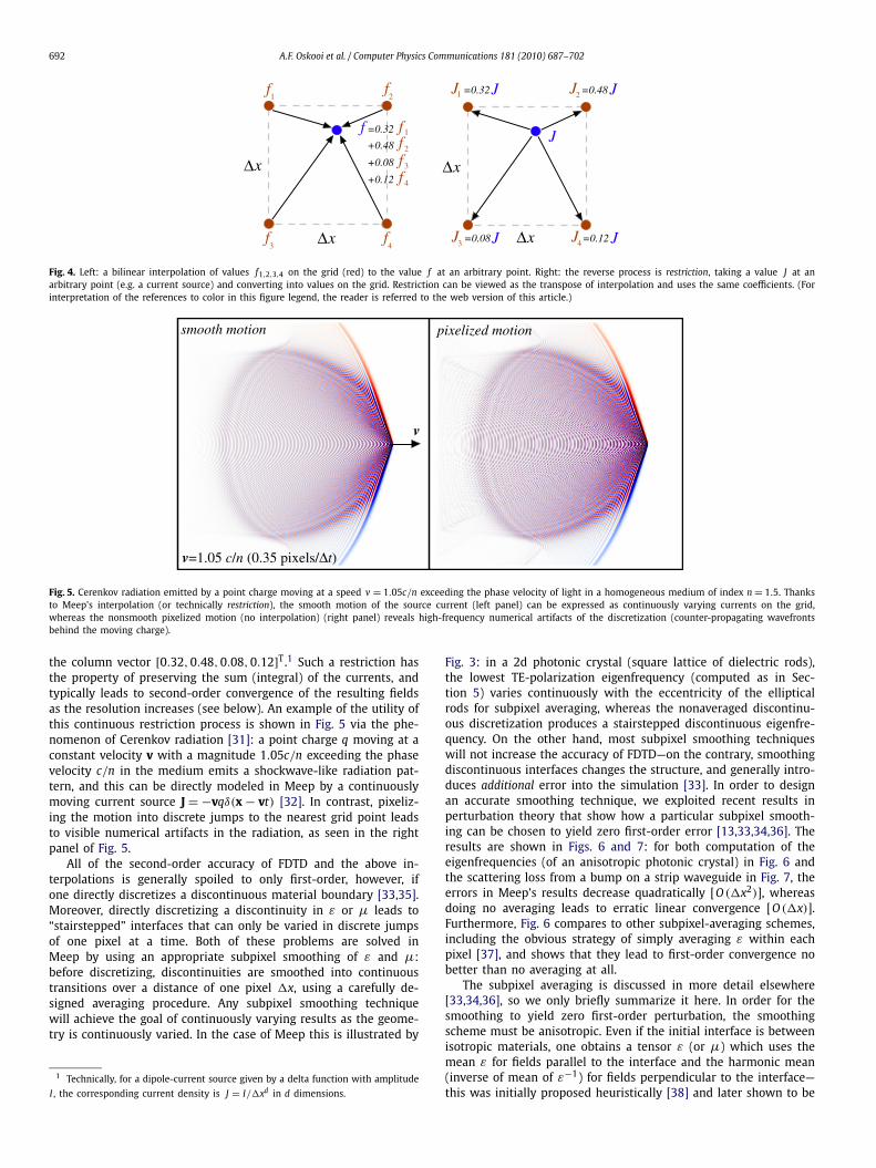
The conceptually reversed process is required for specifyingsources: the current density is specified at some point (for dipolesources) or in some region (for distributed current sources) incontinuous space, and then must be restricted to a correspondingcurrent source on the Yee grid. Meep performs this restriction us-ing exactly the same code (the loop-in-chunks abstraction of Sec-tion 7) and the same weights as the interpolation procedure above.Mathematically, we are exploiting a well-known concept (originat-ing in multigrid methods) that restriction can be defined as thetranspose of interpolation [30]. This is illustrated by a 2d exam-ple in Fig. 4. Suppose that the bilinear interpolation f (blue) offour grid points (red) is f = 0.32 f1 + 0.48 f2 + 0.08 f3 + 0.12 f4,which can be viewed as multiplying a vector of those fields by therow-vector [0.32,0.48,0.08,0.12]. Conversely, if we place a point-dipole current source J (blue) at the same point, it is restricted onthe grid (red) to values J1 = 0.32 J , J2 = 0.48 J , J3 = 0.08 J , andJ4 = 0.12 J as shown in Fig. 4, corresponding to multiplying J by

692 A.F. Oskooi et al. / Computer Physics Communications 181 (2010) 687–702

Fig. 4. Left: a bilinear interpolation of values f1,2,3,4 on the grid (red) to the value f at an arbitrary point. Right: the reverse process is restriction, taking a value J at anarbitrary point (e.g. a current source) and converting into values on the grid. Restriction can be viewed as the transpose of interpolation and uses the same coefficients. (Forinterpretation of the references to color in this figure legend, the reader is referred to the web version of this article.)

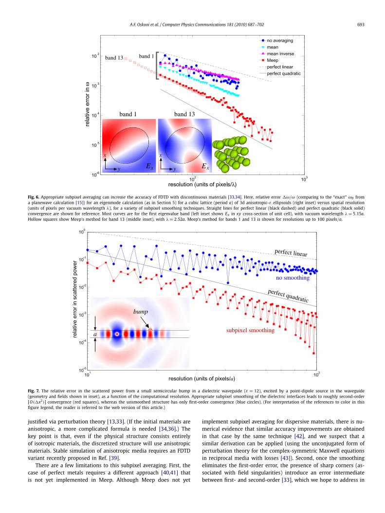
Fig. 5. Cerenkov radiation emitted by a point charge moving at a speed v = 1.05c/n exceeding the phase velocity of light in a homogeneous medium of index n = 1.5. Thanksto Meep’s interpolation (or technically restriction), the smooth motion of the source current (left panel) can be expressed as continuously varying currents on the grid,whereas the nonsmooth pixelized motion (no interpolation) (right panel) reveals high-frequency numerical artifacts of the discretization (counter-propagating wavefrontsbehind the moving charge).

the column vector [0.32,0.48,0.08,0.12]T.1 Such a restriction hasthe property of preserving the sum (integral) of the currents, andtypically leads to second-order convergence of the resulting fieldsas the resolution increases (see below). An example of the utility ofthis continuous restriction process is shown in Fig. 5 via the phe-nomenon of Cerenkov radiation [31]: a point charge q moving at aconstant velocity v with a magnitude 1.05c/n exceeding the phasevelocity c/n in the medium emits a shockwave-like radiation pat-tern, and this can be directly modeled in Meep by a continuouslymoving current source J = −vqδ(x − vt) [32]. In contrast, pixeliz-ing the motion into discrete jumps to the nearest grid point leadsto visible numerical artifacts in the radiation, as seen in the rightpanel of Fig. 5.

All of the second-order accuracy of FDTD and the above in-terpolations is generally spoiled to only first-order, however, ifone directly discretizes a discontinuous material boundary [33,35].Moreover, directly discretizing a discontinuity in ε or μ leads to“stairstepped” interfaces that can only be varied in discrete jumpsof one pixel at a time. Both of these problems are solved inMeep by using an appropriate subpixel smoothing of ε and μ:before discretizing, discontinuities are smoothed into continuoustransitions over a distance of one pixel �x, using a carefully de-signed averaging procedure. Any subpixel smoothing techniquewill achieve the goal of continuously varying results as the geome-try is continuously varied. In the case of Meep this is illustrated by

1 Technically, for a dipole-current source given by a delta function with amplitude

I , the corresponding current density is J = I/�xd in d dimensions.

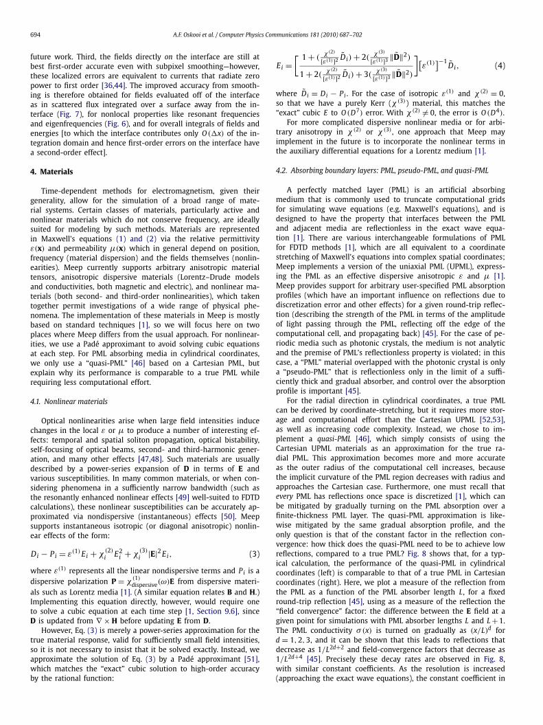
Fig. 3: in a 2d photonic crystal (square lattice of dielectric rods),the lowest TE-polarization eigenfrequency (computed as in Sec-tion 5) varies continuously with the eccentricity of the ellipticalrods for subpixel averaging, whereas the nonaveraged discontinu-ous discretization produces a stairstepped discontinuous eigenfre-quency. On the other hand, most subpixel smoothing techniqueswill not increase the accuracy of FDTD—on the contrary, smoothingdiscontinuous interfaces changes the structure, and generally intro-duces additional error into the simulation [33]. In order to designan accurate smoothing technique, we exploited recent results inperturbation theory that show how a particular subpixel smooth-ing can be chosen to yield zero first-order error [13,33,34,36]. Theresults are shown in Figs. 6 and 7: for both computation of theeigenfrequencies (of an anisotropic photonic crystal) in Fig. 6 andthe scattering loss from a bump on a strip waveguide in Fig. 7, theerrors in Meep’s results decrease quadratically [O (�x2)], whereasdoing no averaging leads to erratic linear convergence [O (�x)].Furthermore, Fig. 6 compares to other subpixel-averaging schemes,including the obvious strategy of simply averaging ε within eachpixel [37], and shows that they lead to first-order convergence nobetter than no averaging at all.

The subpixel averaging is discussed in more detail elsewhere[33,34,36], so we only briefly summarize it here. In order for thesmoothing to yield zero first-order perturbation, the smoothingscheme must be anisotropic. Even if the initial interface is betweenisotropic materials, one obtains a tensor ε (or μ) which uses themean ε for fields parallel to the interface and the harmonic mean(inverse of mean of ε−1) for fields perpendicular to the interface—this was initially proposed heuristically [38] and later shown to be

A.F. Oskooi et al. / Computer Physics Communications 181 (2010) 687–702 693

Fig. 6. Appropriate subpixel averaging can increase the accuracy of FDTD with discontinuous materials [33,34]. Here, relative error �ω/ω (comparing to the “exact” ω0 froma planewave calculation [15]) for an eigenmode calculation (as in Section 5) for a cubic lattice (period a) of 3d anisotropic-ε ellipsoids (right inset) versus spatial resolution(units of pixels per vacuum wavelength λ), for a variety of subpixel smoothing techniques. Straight lines for perfect linear (black dashed) and perfect quadratic (black solid)convergence are shown for reference. Most curves are for the first eigenvalue band (left inset shows Ex in xy cross-section of unit cell), with vacuum wavelength λ = 5.15a.Hollow squares show Meep’s method for band 13 (middle inset), with λ = 2.52a. Meep’s method for bands 1 and 13 is shown for resolutions up to 100 pixels/a.

Fig. 7. The relative error in the scattered power from a small semicircular bump in a dielectric waveguide (ε = 12), excited by a point-dipole source in the waveguide(geometry and fields shown in inset), as a function of the computational resolution. Appropriate subpixel smoothing of the dielectric interfaces leads to roughly second-order[O (�x2)] convergence (red squares), whereas the unsmoothed structure has only first-order convergence (blue circles). (For interpretation of the references to color in thisfigure legend, the reader is referred to the web version of this article.)

justified via perturbation theory [13,33]. (If the initial materials areanisotropic, a more complicated formula is needed [34,36].) Thekey point is that, even if the physical structure consists entirelyof isotropic materials, the discretized structure will use anisotropicmaterials. Stable simulation of anisotropic media requires an FDTDvariant recently proposed in Ref. [39].

There are a few limitations to this subpixel averaging. First, thecase of perfect metals requires a different approach [40,41] thatis not yet implemented in Meep. Although Meep does not yet

implement subpixel averaging for dispersive materials, there is nu-merical evidence that similar accuracy improvements are obtainedin that case by the same technique [42], and we suspect that asimilar derivation can be applied (using the unconjugated form ofperturbation theory for the complex-symmetric Maxwell equationsin reciprocal media with losses [43]). Second, once the smoothingeliminates the first-order error, the presence of sharp corners (as-sociated with field singularities) introduce an error intermediatebetween first- and second-order [33], which we hope to address in

694 A.F. Oskooi et al. / Computer Physics Communications 181 (2010) 687–702

future work. Third, the fields directly on the interface are still atbest first-order accurate even with subpixel smoothing—however,these localized errors are equivalent to currents that radiate zeropower to first order [36,44]. The improved accuracy from smooth-ing is therefore obtained for fields evaluated off of the interfaceas in scattered flux integrated over a surface away from the in-terface (Fig. 7), for nonlocal properties like resonant frequenciesand eigenfrequencies (Fig. 6), and for overall integrals of fields andenergies [to which the interface contributes only O (�x) of the in-tegration domain and hence first-order errors on the interface havea second-order effect].

4. Materials

Time-dependent methods for electromagnetism, given theirgenerality, allow for the simulation of a broad range of mate-rial systems. Certain classes of materials, particularly active andnonlinear materials which do not conserve frequency, are ideallysuited for modeling by such methods. Materials are representedin Maxwell’s equations (1) and (2) via the relative permittivityε(x) and permeability μ(x) which in general depend on position,frequency (material dispersion) and the fields themselves (nonlin-earities). Meep currently supports arbitrary anisotropic materialtensors, anisotropic dispersive materials (Lorentz–Drude modelsand conductivities, both magnetic and electric), and nonlinear ma-terials (both second- and third-order nonlinearities), which takentogether permit investigations of a wide range of physical phe-nomena. The implementation of these materials in Meep is mostlybased on standard techniques [1], so we will focus here on twoplaces where Meep differs from the usual approach. For nonlinear-ities, we use a Padé approximant to avoid solving cubic equationsat each step. For PML absorbing media in cylindrical coordinates,we only use a “quasi-PML” [46] based on a Cartesian PML, butexplain why its performance is comparable to a true PML whilerequiring less computational effort.

4.1. Nonlinear materials

Optical nonlinearities arise when large field intensities inducechanges in the local ε or μ to produce a number of interesting ef-fects: temporal and spatial soliton propagation, optical bistability,self-focusing of optical beams, second- and third-harmonic gener-ation, and many other effects [47,48]. Such materials are usuallydescribed by a power-series expansion of D in terms of E andvarious susceptibilities. In many common materials, or when con-sidering phenomena in a sufficiently narrow bandwidth (such asthe resonantly enhanced nonlinear effects [49] well-suited to FDTDcalculations), these nonlinear susceptibilities can be accurately ap-proximated via nondispersive (instantaneous) effects [50]. Meepsupports instantaneous isotropic (or diagonal anisotropic) nonlin-ear effects of the form:

Di − Pi = ε(1)Ei + χ(2)i E2

i + χ(3)i |E|2 Ei, (3)

where ε(1) represents all the linear nondispersive terms and Pi is adispersive polarization P = χ

(1)

dispersive(ω)E from dispersive materi-als such as Lorentz media [1]. (A similar equation relates B and H.)Implementing this equation directly, however, would require oneto solve a cubic equation at each time step [1, Section 9.6], sinceD is updated from ∇ × H before updating E from D.

However, Eq. (3) is merely a power-series approximation for thetrue material response, valid for sufficiently small field intensities,so it is not necessary to insist that it be solved exactly. Instead, weapproximate the solution of Eq. (3) by a Padé approximant [51],which matches the “exact” cubic solution to high-order accuracyby the rational function:

Ei =[ 1 + (

χ(2)

[ε(1)]2 Di) + 2(χ(3)

[ε(1)]3 ‖D‖2)

1 + 2(χ(2)

[ε(1)]2 Di) + 3(χ(3)

[ε(1)]3 ‖D‖2)

][ε(1)

]−1Di, (4)

where Di = Di − Pi . For the case of isotropic ε(1) and χ(2) = 0,so that we have a purely Kerr (χ(3)) material, this matches the“exact” cubic E to O (D7) error. With χ(2) �= 0, the error is O (D4).

For more complicated dispersive nonlinear media or for arbi-trary anisotropy in χ(2) or χ(3) , one approach that Meep mayimplement in the future is to incorporate the nonlinear terms inthe auxiliary differential equations for a Lorentz medium [1].

4.2. Absorbing boundary layers: PML, pseudo-PML, and quasi-PML

A perfectly matched layer (PML) is an artificial absorbingmedium that is commonly used to truncate computational gridsfor simulating wave equations (e.g. Maxwell’s equations), and isdesigned to have the property that interfaces between the PMLand adjacent media are reflectionless in the exact wave equa-tion [1]. There are various interchangeable formulations of PMLfor FDTD methods [1], which are all equivalent to a coordinatestretching of Maxwell’s equations into complex spatial coordinates;Meep implements a version of the uniaxial PML (UPML), express-ing the PML as an effective dispersive anisotropic ε and μ [1].Meep provides support for arbitrary user-specified PML absorptionprofiles (which have an important influence on reflections due todiscretization error and other effects) for a given round-trip reflec-tion (describing the strength of the PML in terms of the amplitudeof light passing through the PML, reflecting off the edge of thecomputational cell, and propagating back) [45]. For the case of pe-riodic media such as photonic crystals, the medium is not analyticand the premise of PML’s reflectionless property is violated; in thiscase, a “PML” material overlapped with the photonic crystal is onlya “pseudo-PML” that is reflectionless only in the limit of a suffi-ciently thick and gradual absorber, and control over the absorptionprofile is important [45].

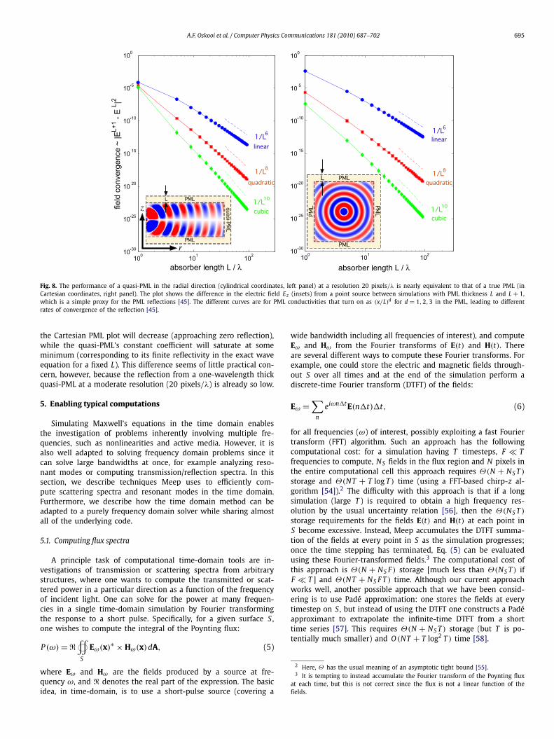
For the radial direction in cylindrical coordinates, a true PMLcan be derived by coordinate-stretching, but it requires more stor-age and computational effort than the Cartesian UPML [52,53],as well as increasing code complexity. Instead, we chose to im-plement a quasi-PML [46], which simply consists of using theCartesian UPML materials as an approximation for the true ra-dial PML. This approximation becomes more and more accurateas the outer radius of the computational cell increases, becausethe implicit curvature of the PML region decreases with radius andapproaches the Cartesian case. Furthermore, one must recall thatevery PML has reflections once space is discretized [1], which canbe mitigated by gradually turning on the PML absorption over afinite-thickness PML layer. The quasi-PML approximation is like-wise mitigated by the same gradual absorption profile, and theonly question is that of the constant factor in the reflection con-vergence: how thick does the quasi-PML need to be to achieve lowreflections, compared to a true PML? Fig. 8 shows that, for a typ-ical calculation, the performance of the quasi-PML in cylindricalcoordinates (left) is comparable to that of a true PML in Cartesiancoordinates (right). Here, we plot a measure of the reflection fromthe PML as a function of the PML absorber length L, for a fixedround-trip reflection [45], using as a measure of the reflection the“field convergence” factor: the difference between the E field at agiven point for simulations with PML absorber lengths L and L +1.The PML conductivity σ(x) is turned on gradually as (x/L)d ford = 1,2,3, and it can be shown that this leads to reflections thatdecrease as 1/L2d+2 and field-convergence factors that decrease as1/L2d+4 [45]. Precisely these decay rates are observed in Fig. 8,with similar constant coefficients. As the resolution is increased(approaching the exact wave equations), the constant coefficient in

A.F. Oskooi et al. / Computer Physics Communications 181 (2010) 687–702 695

Fig. 8. The performance of a quasi-PML in the radial direction (cylindrical coordinates, left panel) at a resolution 20 pixels/λ is nearly equivalent to that of a true PML (inCartesian coordinates, right panel). The plot shows the difference in the electric field Ez (insets) from a point source between simulations with PML thickness L and L + 1,which is a simple proxy for the PML reflections [45]. The different curves are for PML conductivities that turn on as (x/L)d for d = 1,2,3 in the PML, leading to differentrates of convergence of the reflection [45].

the Cartesian PML plot will decrease (approaching zero reflection),while the quasi-PML’s constant coefficient will saturate at someminimum (corresponding to its finite reflectivity in the exact waveequation for a fixed L). This difference seems of little practical con-cern, however, because the reflection from a one-wavelength thickquasi-PML at a moderate resolution (20 pixels/λ) is already so low.

5. Enabling typical computations

Simulating Maxwell’s equations in the time domain enablesthe investigation of problems inherently involving multiple fre-quencies, such as nonlinearities and active media. However, it isalso well adapted to solving frequency domain problems since itcan solve large bandwidths at once, for example analyzing reso-nant modes or computing transmission/reflection spectra. In thissection, we describe techniques Meep uses to efficiently com-pute scattering spectra and resonant modes in the time domain.Furthermore, we describe how the time domain method can beadapted to a purely frequency domain solver while sharing almostall of the underlying code.

5.1. Computing flux spectra

A principle task of computational time-domain tools are in-vestigations of transmission or scattering spectra from arbitrarystructures, where one wants to compute the transmitted or scat-tered power in a particular direction as a function of the frequencyof incident light. One can solve for the power at many frequen-cies in a single time-domain simulation by Fourier transformingthe response to a short pulse. Specifically, for a given surface S ,one wishes to compute the integral of the Poynting flux:

P (ω) = ��

S

Eω(x)∗ × Hω(x)dA, (5)

where Eω and Hω are the fields produced by a source at fre-quency ω, and � denotes the real part of the expression. The basicidea, in time-domain, is to use a short-pulse source (covering a

wide bandwidth including all frequencies of interest), and computeEω and Hω from the Fourier transforms of E(t) and H(t). Thereare several different ways to compute these Fourier transforms. Forexample, one could store the electric and magnetic fields through-out S over all times and at the end of the simulation perform adiscrete-time Fourier transform (DTFT) of the fields:

Eω =∑

n

eiωn�tE(n�t)�t, (6)

for all frequencies (ω) of interest, possibly exploiting a fast Fouriertransform (FFT) algorithm. Such an approach has the followingcomputational cost: for a simulation having T timesteps, F � Tfrequencies to compute, N S fields in the flux region and N pixels inthe entire computational cell this approach requires Θ(N + N S T )

storage and Θ(NT + T log T ) time (using a FFT-based chirp-z al-gorithm [54]).2 The difficulty with this approach is that if a longsimulation (large T ) is required to obtain a high frequency res-olution by the usual uncertainty relation [56], then the Θ(N S T )

storage requirements for the fields E(t) and H(t) at each point inS become excessive. Instead, Meep accumulates the DTFT summa-tion of the fields at every point in S as the simulation progresses;once the time stepping has terminated, Eq. (5) can be evaluatedusing these Fourier-transformed fields.3 The computational cost ofthis approach is Θ(N + N S F ) storage [much less than Θ(N S T ) ifF � T ] and Θ(NT + N S F T ) time. Although our current approachworks well, another possible approach that we have been consid-ering is to use Padé approximation: one stores the fields at everytimestep on S , but instead of using the DTFT one constructs a Padéapproximant to extrapolate the infinite-time DTFT from a shorttime series [57]. This requires Θ(N + N S T ) storage (but T is po-tentially much smaller) and O (NT + T log2 T ) time [58].

2 Here, Θ has the usual meaning of an asymptotic tight bound [55].3 It is tempting to instead accumulate the Fourier transform of the Poynting flux

at each time, but this is not correct since the flux is not a linear function of thefields.

696 A.F. Oskooi et al. / Computer Physics Communications 181 (2010) 687–702

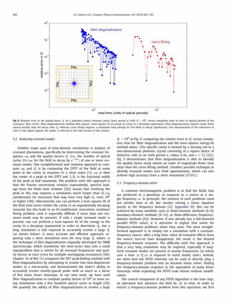
Fig. 9. Relative error in the quality factor Q for a photonic-crystal resonant cavity (inset, period a) with Q ∼ 106, versus simulation time in units of optical periods of theresonance. Blue circles: filter-diagonalization method. Red squares: least-squares fit of energy in cavity to a decaying exponential. Filter-diagonalization requires many feweroptical periods than the decay time Q , whereas curve fitting requires a simulation long enough for the fields to decay significantly. (For interpretation of the references tocolor in this figure legend, the reader is referred to the web version of this article.)

5.2. Analyzing resonant modes

Another major goal of time-domain simulations is analysis ofresonant phenomena, specifically by determining the resonant fre-quency ω0 and the quality factors Q (i.e., the number of opticalcycles 2π/ω0 for the field to decay by e−2π ) of one or more res-onant modes. One straightforward and common approach to com-pute ω0 and Q is by computing the DTFT of the field at somepoint in the cavity in response to a short pulse [1]: ω0 is thenthe center of a peak in the DTFT and 1/Q is the fractional widthof the peak at half maximum. The problem with this approach isthat the Fourier uncertainty relation (equivalently, spectral leak-age from the finite time window [56]) means that resolving thepeak in this way requires a simulation much longer than Q /ω0(problematic for structures that may have very high Q , even 109

or higher [59]). Alternatively, one can perform a least squares fit ofthe field time-series within the cavity to an exponentially decayingsinusoid, but this leads to an ill-conditioned, nonconvex, nonlinearfitting problem (and is especially difficult if more than one res-onant mode may be present). If only a single resonant mode ispresent, one can perform a least-squares fit of the energy in thecavity to a decaying exponential in order to determine Q , but along simulation is still required to accurately resolve a large Q(as shown below). A more accurate and efficient approach, re-quiring only a short simulation even for very large Q values, isthe technique of filter diagonalization originally developed for NMRspectroscopy, which transforms the time-series data into a smalleigenproblem that is solved for all resonant frequencies and qual-ity factors at once (even for multiple overlapping resonances) [60].Chapter 16 of Ref. [1] compared the DFT peak-finding method withfilter-diagonalization by attempting to resolve two near-degeneratemodes in a microcavity, and demonstrated the latter’s ability toaccurately resolve closely-spaced peaks with as much as a factorof five times fewer timesteps. In our own work, we have usedfilter diagonalization to compute quality factors of 108 or more us-ing simulations only a few hundred optical cycles in length [59].We quantify the ability of filter diagonalization to resolve a large

Q ∼ 106 in Fig. 9, comparing the relative error in Q versus simula-tion time for filter diagonalization and the least-squares energy-fitmethod above. (The specific cavity is formed by a missing rod in atwo-dimensional photonic crystal consisting of a square lattice ofdielectric rods in air with period a, radius 0.2a, and ε = 12 [22].)Fig. 9 demonstrates that filter diagonalization is able to identifythe quality factor using almost an order of magnitude fewer timesteps than the curve fitting method. (Another possible technique toidentify resonant modes uses Padé approximants, which can alsoachieve high accuracy from a short simulation [57,61].)

5.3. Frequency-domain solver

A common electromagnetic problem is to find the fields thatare produced in a geometry in response to a source at a sin-gle frequency ω. In principle, the solution of such problems neednot involve time at all, but involve solving a linear equationpurely in the frequency domain [22, Appendix D]; this can beachieved by many methods, such as finite-element methods [6–8],boundary-element methods [9–12], or finite-difference frequency-domain methods [62]. However, if one already has a full-featuredparallel FDTD solver, it is attractive to exploit that solver forfrequency-domain problems when they arise. The most straight-forward approach is to simply run a simulation with a constant-frequency source—after a long time, when all transient effects fromthe source turn-on have disappeared, the result is the desiredfrequency-domain response. The difficulty with this approach isthat a very long simulation may be required, especially if long-lived resonant modes are present at nearby frequencies (in whichcase a time Q /ω is required to reach steady state). Instead,we show how the FDTD timestep can be used to directly plug afrequency-domain problem into an iterative linear solver, findingthe frequency-domain response in the equivalent of many fewertimesteps while exploiting the FDTD code almost without modifi-cation.

The central component of any FDTD algorithm is the time step:an operation that advances the field by �t in time. In order toextract a frequency-domain problem from this operation, we first

A.F. Oskooi et al. / Computer Physics Communications 181 (2010) 687–702 697

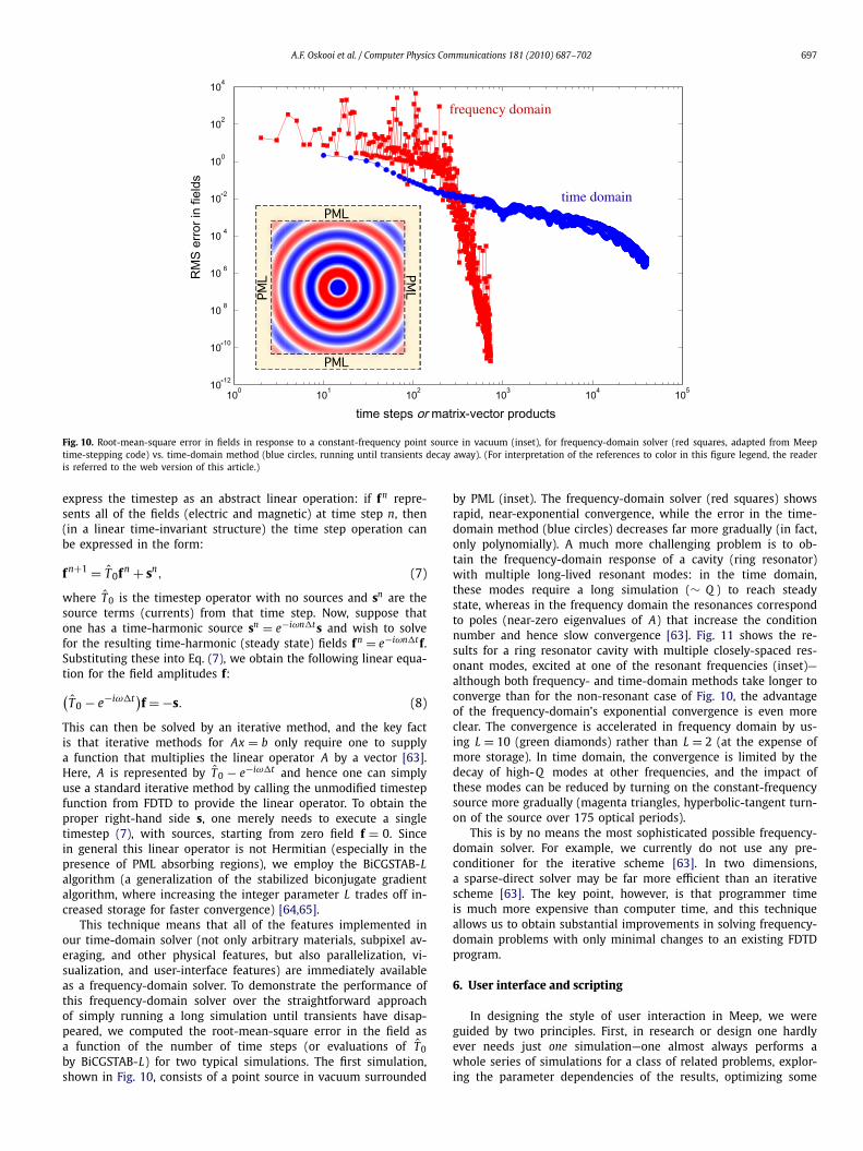
Fig. 10. Root-mean-square error in fields in response to a constant-frequency point source in vacuum (inset), for frequency-domain solver (red squares, adapted from Meeptime-stepping code) vs. time-domain method (blue circles, running until transients decay away). (For interpretation of the references to color in this figure legend, the readeris referred to the web version of this article.)

express the timestep as an abstract linear operation: if fn repre-sents all of the fields (electric and magnetic) at time step n, then(in a linear time-invariant structure) the time step operation canbe expressed in the form:

fn+1 = T0fn + sn, (7)

where T0 is the timestep operator with no sources and sn are thesource terms (currents) from that time step. Now, suppose thatone has a time-harmonic source sn = e−iωn�ts and wish to solvefor the resulting time-harmonic (steady state) fields fn = e−iωn�tf.Substituting these into Eq. (7), we obtain the following linear equa-tion for the field amplitudes f:

(T0 − e−iω�t)f = −s. (8)

This can then be solved by an iterative method, and the key factis that iterative methods for Ax = b only require one to supplya function that multiplies the linear operator A by a vector [63].Here, A is represented by T0 − e−iω�t and hence one can simplyuse a standard iterative method by calling the unmodified timestepfunction from FDTD to provide the linear operator. To obtain theproper right-hand side s, one merely needs to execute a singletimestep (7), with sources, starting from zero field f = 0. Sincein general this linear operator is not Hermitian (especially in thepresence of PML absorbing regions), we employ the BiCGSTAB-Lalgorithm (a generalization of the stabilized biconjugate gradientalgorithm, where increasing the integer parameter L trades off in-creased storage for faster convergence) [64,65].

This technique means that all of the features implemented inour time-domain solver (not only arbitrary materials, subpixel av-eraging, and other physical features, but also parallelization, vi-sualization, and user-interface features) are immediately availableas a frequency-domain solver. To demonstrate the performance ofthis frequency-domain solver over the straightforward approachof simply running a long simulation until transients have disap-peared, we computed the root-mean-square error in the field asa function of the number of time steps (or evaluations of T0by BiCGSTAB-L) for two typical simulations. The first simulation,shown in Fig. 10, consists of a point source in vacuum surrounded

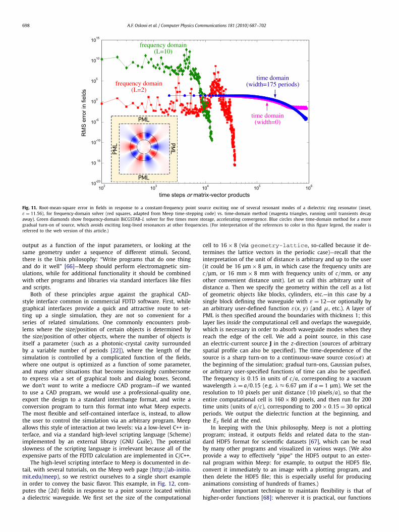
by PML (inset). The frequency-domain solver (red squares) showsrapid, near-exponential convergence, while the error in the time-domain method (blue circles) decreases far more gradually (in fact,only polynomially). A much more challenging problem is to ob-tain the frequency-domain response of a cavity (ring resonator)with multiple long-lived resonant modes: in the time domain,these modes require a long simulation (∼ Q ) to reach steadystate, whereas in the frequency domain the resonances correspondto poles (near-zero eigenvalues of A) that increase the conditionnumber and hence slow convergence [63]. Fig. 11 shows the re-sults for a ring resonator cavity with multiple closely-spaced res-onant modes, excited at one of the resonant frequencies (inset)—although both frequency- and time-domain methods take longer toconverge than for the non-resonant case of Fig. 10, the advantageof the frequency-domain’s exponential convergence is even moreclear. The convergence is accelerated in frequency domain by us-ing L = 10 (green diamonds) rather than L = 2 (at the expense ofmore storage). In time domain, the convergence is limited by thedecay of high-Q modes at other frequencies, and the impact ofthese modes can be reduced by turning on the constant-frequencysource more gradually (magenta triangles, hyperbolic-tangent turn-on of the source over 175 optical periods).

This is by no means the most sophisticated possible frequency-domain solver. For example, we currently do not use any pre-conditioner for the iterative scheme [63]. In two dimensions,a sparse-direct solver may be far more efficient than an iterativescheme [63]. The key point, however, is that programmer timeis much more expensive than computer time, and this techniqueallows us to obtain substantial improvements in solving frequency-domain problems with only minimal changes to an existing FDTDprogram.

6. User interface and scripting

In designing the style of user interaction in Meep, we wereguided by two principles. First, in research or design one hardlyever needs just one simulation—one almost always performs awhole series of simulations for a class of related problems, explor-ing the parameter dependencies of the results, optimizing some

698 A.F. Oskooi et al. / Computer Physics Communications 181 (2010) 687–702

Fig. 11. Root-mean-square error in fields in response to a constant-frequency point source exciting one of several resonant modes of a dielectric ring resonator (inset,ε = 11.56), for frequency-domain solver (red squares, adapted from Meep time-stepping code) vs. time-domain method (magenta triangles, running until transients decayaway). Green diamonds show frequency-domain BiCGSTAB-L solver for five times more storage, accelerating convergence. Blue circles show time-domain method for a moregradual turn-on of source, which avoids exciting long-lived resonances at other frequencies. (For interpretation of the references to color in this figure legend, the reader isreferred to the web version of this article.)

output as a function of the input parameters, or looking at thesame geometry under a sequence of different stimuli. Second,there is the Unix philosophy: “Write programs that do one thingand do it well” [66]—Meep should perform electromagnetic sim-ulations, while for additional functionality it should be combinedwith other programs and libraries via standard interfaces like filesand scripts.

Both of these principles argue against the graphical CAD-style interface common in commercial FDTD software. First, whilegraphical interfaces provide a quick and attractive route to set-ting up a single simulation, they are not so convenient for aseries of related simulations. One commonly encounters prob-lems where the size/position of certain objects is determined bythe size/position of other objects, where the number of objects isitself a parameter (such as a photonic-crystal cavity surroundedby a variable number of periods [22]), where the length of thesimulation is controlled by a complicated function of the fields,where one output is optimized as a function of some parameter,and many other situations that become increasingly cumbersometo express via a set of graphical tools and dialog boxes. Second,we don’t want to write a mediocre CAD program—if we wantedto use a CAD program, we would use a professional-quality one,export the design to a standard interchange format, and write aconversion program to turn this format into what Meep expects.The most flexible and self-contained interface is, instead, to allowthe user to control the simulation via an arbitrary program. Meepallows this style of interaction at two levels: via a low-level C++ in-terface, and via a standard high-level scripting language (Scheme)implemented by an external library (GNU Guile). The potentialslowness of the scripting language is irrelevant because all of theexpensive parts of the FDTD calculation are implemented in C/C++.

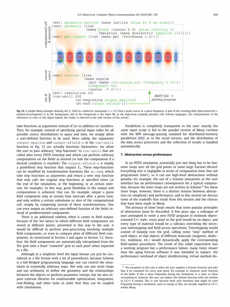
The high-level scripting interface to Meep is documented in de-tail, with several tutorials, on the Meep web page (http://ab-initio.mit.edu/meep), so we restrict ourselves to a single short examplein order to convey the basic flavor. This example, in Fig. 12, com-putes the (2d) fields in response to a point source located withina dielectric waveguide. We first set the size of the computational

cell to 16 × 8 (via geometry-lattice, so-called because it de-termines the lattice vectors in the periodic case)—recall that theinterpretation of the unit of distance is arbitrary and up to the user(it could be 16 μm × 8 μm, in which case the frequency units arec/μm, or 16 mm × 8 mm with frequency units of c/mm, or anyother convenient distance unit). Let us call this arbitrary unit ofdistance a. Then we specify the geometry within the cell as a listof geometric objects like blocks, cylinders, etc.—in this case by asingle block defining the waveguide with ε = 12—or optionally byan arbitrary user-defined function ε(x, y) (and μ, etc.). A layer ofPML is then specified around the boundaries with thickness 1; thislayer lies inside the computational cell and overlaps the waveguide,which is necessary in order to absorb waveguide modes when theyreach the edge of the cell. We add a point source, in this casean electric-current source J in the z-direction (sources of arbitraryspatial profile can also be specified). The time-dependence of thesource is a sharp turn-on to a continuous-wave source cos(ωt) atthe beginning of the simulation; gradual turn-ons, Gaussian pulses,or arbitrary user-specified functions of time can also be specified.The frequency is 0.15 in units of c/a, corresponding to a vacuumwavelength λ = a/0.15 (e.g. λ ≈ 6.67 μm if a = 1 μm). We set theresolution to 10 pixels per unit distance (10 pixels/a), so that theentire computational cell is 160 × 80 pixels, and then run for 200time units (units of a/c), corresponding to 200 × 0.15 = 30 opticalperiods. We output the dielectric function at the beginning, andthe Ez field at the end.

In keeping with the Unix philosophy, Meep is not a plottingprogram; instead, it outputs fields and related data to the stan-dard HDF5 format for scientific datasets [67], which can be readby many other programs and visualized in various ways. (We alsoprovide a way to effectively “pipe” the HDF5 output to an exter-nal program within Meep: for example, to output the HDF5 file,convert it immediately to an image with a plotting program, andthen delete the HDF5 file; this is especially useful for producinganimations consisting of hundreds of frames.)

Another important technique to maintain flexibility is that ofhigher-order functions [68]: wherever it is practical, our functions

A.F. Oskooi et al. / Computer Physics Communications 181 (2010) 687–702 699

Fig. 12. A simple Meep example showing the Ez field in a dielectric waveguide (ε = 12) from a point source at a given frequency. A plot of the resulting field (blue/white/red =positive/zero/negative) is in the background, and in the foreground is the input file in the high-level scripting interface (the Scheme language). (For interpretation of thereferences to color in this figure legend, the reader is referred to the web version of this article.)

take functions as arguments instead of (or in addition to) numbers.Thus, for example, instead of specifying special input codes for allpossible source distributions in space and time, we simply allowa user-defined function to be used. More subtly, the argumentsoutput-epsilon and output-efield-z to the run-untilfunction in Fig. 12 are actually functions themselves: we allowthe user to pass arbitrary “step functions” to run-until that arecalled after every FDTD timestep and which can perform arbitrarycomputations on the fields as desired (or halt the computation if adesired condition is reached). The output-efield-z is simplya predefined step function that outputs Ez . These step-functionscan be modified by transformation functions like at-end, whichtake step functions as arguments and return a new step functionthat only calls the original step functions at specified times (atthe end of the simulation, or the beginning, or at certain inter-vals, for example). In this way, great flexibility in the output andcomputations is achieved. One can, for example, output a givenfield component only at certain time intervals after a given time,and only within a certain subvolume or slice of the computationalcell, simply by composing several of these transformations. Onecan even output an arbitrary user-defined function of the fields in-stead of predetermined components.

There is an additional subtlety when it comes to field output,because of the Yee lattice in which different field components arestored at different points; presented in this way to the user, itwould be difficult to perform post-processing involving multiplefield components, or even to compare plots of different field com-ponents. As mentioned in Section 3 and again in Section 7.2, there-fore, the field components are automatically interpolated from theYee grid onto a fixed “centered” grid in each pixel when exportedto a file.

Although at a simplistic level the input format can just be con-sidered as a file format with a lot of parentheses, because Schemeis a full-fledged programming language one can control the simu-lation in essentially arbitrary ways. Not only can one write loopsand use arithmetic to define the geometry and the relationshipsbetween the objects or perform parameter sweeps, but we also ex-pose external libraries for multivariable optimization, integration,root-finding, and other tasks in order that they can be coupledwith simulations.

Parallelism is completely transparent to the user: exactly thesame input script is fed to the parallel version of Meep (writtenwith the MPI message-passing standard for distributed-memoryparallelism [69]) as to the serial version, and the distribution ofthe data across processors and the collection of results is handledautomatically.

7. Abstraction versus performance

In an FDTD simulation, essentially just one thing has to be fast:inner loops over all the grid points or some large fraction thereof.Everything else is negligible in terms of computation time (but notprogrammer time!), so it can use high-level abstractions withoutpenalty—for example, the use of a Scheme interpreter as the userinterface has no performance consequences for a typical computa-tion, because the inner loops are not written in Scheme.4 For theseinner loops, however, there is a distinct tension between abstrac-tion (or simplicity) and performance, and in this section we discusssome of the tradeoffs that result from this tension and the choicesthat have been made in Meep.

The primacy of inner loops means that some popular principlesof abstraction must be discarded. A few years ago, a colleague ofours attempted to write a new FDTD program in textbook object-oriented C++ style: every pixel in the grid would be an object, andevery type of material would be a subclass overriding the neces-sary timestepping and field-access operations. Timestepping wouldconsist of looping over the grid, calling some “step” method ofeach object, so that objects of different materials (magnetic, dielec-tric, nonlinear, etc.) would dynamically apply the correspondingfield-update procedures. The result of this noble experiment wasa working program but a performance failure, many times slowerthan the aging Fortran software it was intended to replace: theperformance overhead of object dereferencing, virtual method dis-

4 The exception to this rule is when the user supplies a Scheme function and asksthat it be evaluated for every grid point, for example to integrate some functionof the fields. If this is done frequently during the simulation, it is slow; in thesecircumstances, however, the user can replace the Scheme function with one writtenin C/C++ if needed. This is rare because most such functions that might be usedfrequently during a simulation, such as energy or flux, are already supplied in C/C++within Meep.

700 A.F. Oskooi et al. / Computer Physics Communications 181 (2010) 687–702

patch, and function calls in the inner loop overwhelmed all otherconsiderations. In Meep, each field’s components are stored as sim-ple linear arrays of floating-point numbers in row-major (C) order(parallel-array data structures worthy of Fortran 66), and there areseparate inner loops for each type of material (more on this be-low). In a simple experiment on a 2.8 GHz Intel Core 2 CPU, merelymoving the if statements for the different material types intothese inner loops decreased Meep’s performance by a factor of twoin a typical 3d calculation and by a factor of six in 2d (where thecalculations are simpler and hence the overhead of the condition-als is more significant). The cost of the conditionals, including thecost of mispredicted branches and subsequent pipeline stalls [70]along with the frustration of compiler unrolling and vectorization,easily overwhelmed the small cost of computing, e.g., ∇ × H at asingle point.

7.1. Timestepping and cache tradeoffs

One of the dominant factors in performance on modern com-puter systems is not arithmetic, but memory: random memoryaccess is far slower than arithmetic, and the organization of mem-ory into a hierarchy of caches is designed to favor locality of ac-cess [70]. That is, one should organize the computation so thatas much work as possible is done with a given datum once it isfetched (temporal locality) and so that subsequent data that areread or written are located nearby in memory (spatial locality).The optimal strategies to exploit both kinds of locality, however,appear to lead to sacrifices of abstraction and code simplicity sosevere that we have chosen instead to sacrifice some potential per-formance in the name of simplicity.

As it is typically described, the FDTD algorithm has very lit-tle temporal locality: the field at each point is advanced in time by�t , and then is not modified again until all the fields at every otherpoint in the computational cell have been advanced. In order togain temporal locality, one must employ asynchronous timestepping:essentially, points in small regions of space are advanced severalsteps in time before advancing points far away, since over a shorttime interval the effects of far-away points cannot be felt. A de-tailed analysis of the characteristics of this problem, as well as abeautiful “cache-oblivious” algorithm that automatically exploits acache of any size for grids of any dimensionality, is described inRef. [71]. On the other hand, an important part of Meep’s usabilityis the abstraction that the user can perform arbitrary computationsor output using the fields in any spatial region at any time, whichseems incompatible with the fields at different points in space be-ing out-of-sync until a predetermined end of the computation. Thebookkeeping difficulty of reconciling these two viewpoints led usto reject the asynchronous approach, despite its potential benefits.

However, there may appear to be at least a small amount oftemporal locality in the synchronous FDTD algorithm: first B is ad-vanced from ∇ × E, then H is computed from B and μ, then D isadvanced from ∇ × H, then E is computed from D and ε. Sincemost fields are used at least once after they are advanced, surelythe updates of the different fields can be merged into a single loop,for example advancing D at a point and then immediately com-puting E at the same point—the D field need not even be stored.Furthermore, since by merging the updates one is accessing sev-eral fields around the same point at the same time, perhaps onecan gain spatial locality by interleaving the data, say by storing anarray of (E,H, ε,μ) tuples instead of separate arrays. Meep doesnot do either of these things, however, for two reasons, the firstof which is more fundamental. As is well known, one cannot eas-ily merge the B and H updates with the D and E updates at thesame point, because the discretized ∇ × operation is nonlocal (in-volves multiple grid points)—this is why one normally updates Heverywhere in space before updating D from ∇ × H, because in

computing ∇ × H one uses the values of H at different grid pointsand all of them must be in sync. A similar reasoning, however,applies to updating E from D and H from B, once the possibilityof anisotropic materials is included—because the Yee grid storesdifferent field components at different locations, any accurate han-dling of off-diagonal susceptibilities must also inevitably involvefields at multiple points (as in Ref. [39]). To handle this, D must bestored explicitly and the update of E from D must take place af-ter D has been updated everywhere, in a separate loop. And sinceeach field is updated in a separate loop, the spatial-locality moti-vation to merge the field data structures rather than using parallelarrays is largely removed.

Of course, not all simulations involve anisotropic materials—although they appear even in many simulations with nominallyisotropic materials thanks to the subpixel averaging discussed inSection 3—but this leads to the second practical problem withmerging the E and D (or H and B) update loops: the combina-torial explosion of the possible material cases. The update of Dfrom ∇ × H must handle 16 possible cases, each of which is a sep-arate loop (see above for the cost of putting conditionals inside theloops): with or without PML (4 cases, depending upon the numberof PML conductivities and their orientation relative to the field),with or without conductivity, and with the derivative of two Hcomponents (3d) or only one H component (2d TE polarization).The update of E from D involves 12 cases: with or without PML(2 cases, distinct from those in the D update), the number of off-diagonal ε−1 components (3 cases: 0, 1, or 2), and with or withoutnonlinearity (2 cases). If we attempted to join these into a sin-gle loop, we would have 16 × 12 = 192 cases, a code-maintenanceheadache. (Note that the multiplicity of PML cases comes from thefact that, including the corners of the computational cell, we mighthave 0 to 3 directions of PML, and the orientation of the PML di-rections relative to a given field component matters greatly.)

The performance penalty of separate E and D (or H and B)updates appears to be modest. Even if, by somehow merging theloops, one assumes that the time to compute E = ε−1D could be-come zero, benchmarking the relative time spent in this operationindicates that a typical 3d transmission calculation would be ac-celerated by only around 30% (and less in 2d).

7.2. The loop-in-chunks abstraction

Finally, let us briefly mention a central abstraction that, whilenot directly visible to end-users of Meep, is key to the efficiencyand maintainability of large portions of the software (field output,current sources, flux/energy computations and other field integrals,and so on). The purpose of this abstraction is to mask the com-plexity of the partitioning of the computational cell into overlap-ping chunks connected by symmetries, communication, and otherboundary conditions as described in Section 2.

Consider the output of the fields at a given timestep to an HDF5datafile. Meep provides a routine get-field-pt that, given apoint in space, interpolates it onto the Yee grid and returns a de-sired field component at that point. In addition to interpolation,this routine must also transform the point onto a chunk that isactually stored (using rotations, periodicity, etc.) and communicatethe data from another processor if necessary. If the point is ona boundary between two chunks, the interpolation process mayinvolve multiple chunks, multiple rotations, etc., and communica-tions from multiple processors. Because this process involves onlya single point, it is not easily parallelizable. Now, to output thefields everywhere in some region to a file, one approach is to sim-ply call get-field-pt for every point in a grid for that regionand output the results, but this turns out to be tremendously slowbecause of the repeated transformations and communications forevery single point. We nevertheless want to interpolate fields for

A.F. Oskooi et al. / Computer Physics Communications 181 (2010) 687–702 701

output rather than dumping the raw Yee grid, because it is mucheasier for post-processing if the different field components are in-terpolated onto the same grid; also, to maintain transparency offeatures like symmetry one would like to be able to output thewhole computational cell (or an arbitrary subset) even if only apart of it is stored. Almost exactly the same problems arise for in-tegrating things like flux E × H or energy or user-defined functionsof the fields (noting that functions combining multiple field com-ponents require interpolation), and also for implementing volume(or line, or surface) sources which must be projected onto the gridin some arbitrary volume.

One key to solving this difficulty is to realize that, when thefield in some volume V is needed (for output, integration, and soon), the rotations, communications, etc. for points in V are iden-tical for all the points in the intersection of V with some chunk(or one of its rotations/translations). The second is to realize that,when interpolation is needed, there is a particular grid for whichinterpolation is easy: for owned points of the centered grid (Sec-tion 2) lying at the center of each pixel, it is always possible tointerpolate from fields on any Yee grid without any inter-chunkcommunication and by a simple equal-weight averaging of at most2d points in d dimensions.

The combination of these two observations leads to the loop-in-chunks abstraction. Given a (convex rectilinear) volume V anda given grid (either centered, or one of the Yee-field grids),it computes the intersection of all the chunks and their rota-tions/translations with V . For each intersection it invokes a caller-specified function, passing the portion of the chunk, the necessaryrotations (etc.) of the fields, and interpolation weights (if needed,for the boundary of V ). That function then processes the specifiedportion of the chunk (for example, outputting it to the correspond-ing portion of a file, or integrating the desired fields). All of thiscan proceed in parallel (with each processor considering only thosechunks stored locally). This is (relatively) fast because the rotations,interpolations, and so on are computed only once per chunk inter-section, while the inner loop over all grid points in each chunk canbe as tight as necessary. Moreover, all of the rather complicatedand error-prone logic involved in computing V ’s intersection withthe chunks (e.g., special care is required to ensure that each con-ceptual grid point is processed exactly once despite chunk overlapsand symmetries) is localized to one place in the source code; fieldoutput, integration, sources, and other functions of the fields areisolated from this complexity.

8. Concluding remarks

We have reviewed in this paper a number of the unusual imple-mentation details of Meep that distinguish our software packagefrom standard textbook FDTD methods. Beginning with a discus-sion of the fundamental structural unit of chunks that constitutethe Yee grid and enable parallelization: we provided an overviewof Meep’s core design philosophy of creating an illusion of con-tinuous space and time for inputs and outputs; we explained andmotivated the somewhat unusual design intricacies of nonlinearmaterials and PMLs; we discussed important aspects of Meep’scomputational methods for flux spectra and resonant modes; wedemonstrated the formulation of a frequency-domain solver requir-ing only minimal modifications to the underlying time-steppingalgorithm. In addition to the inner workings of Meep’s internalstructure, we reviewed how such features are accessible to usersvia an external scripting interface.

We believe that a free/open-source, full-featured FDTD pack-age like Meep can play a vital role in enabling new research inelectromagnetic phenomena. Not only does it provide a low bar-rier to entry for standard FDTD simulations, but the simplicity ofthe FDTD algorithm combined with access to the source code of-

fers an easy route to investigate new physical phenomena coupledwith electromagnetism. For example, we have colleagues workingon coupling multi-level atoms to electromagnetism within Meepfor modeling lasing and saturable absorption, adapting publishedtechniques from our and other groups [16–20], but also includingnew physics such as diffusion of excited gases. Other colleagueshave modified Meep for modeling gyromagnetic media in order todesign new classes of “one-way” waveguides [72]. Meep is evenbeing used to simulate the quantum phenomena of Casimir forces(from quantum vacuum fluctuations, which can be computed fromclassical Green’s functions) [73,74]—in fact, this was possible with-out any modifications of the Meep code due to the flexibility ofMeep’s scripting interface. We hope that other researchers, withthe help of the understanding of Meep’s architecture that this pa-per provides, will be able to adapt Meep to future phenomena thatwe have not yet envisioned.

Acknowledgements

This work was supported in part by the Materials ResearchScience and Engineering Center program of the National ScienceFoundation under Grant Nos. DMR-9400334 and DMR-0819762, bythe Army Research Office through the Institute for Soldier Nan-otechnologies under contract DAAD-19-02-D0002, and also by Dr.Dennis Healy of DARPA MTO under award N00014-05-1-0700 ad-ministered by the Office of Naval Research. We are also gratefulto A.W. Rodriguez and A.P. McCauley for their efforts to general-ize Meep for quantum-Casimir problems, S.L. Chua for his work ondispersive and multi-level materials, and Y. Chong for early supportin Meep for gyrotropic media.

References

[1] A. Taflove, S.C. Hagness, Computational Electrodynamics: The Finite-DifferenceTime-Domain Method, 3rd ed., Artech, Norwood, MA, 2005.

[2] K.S. Kunz, R.J. Luebbers, The Finite-Difference Time-Domain Method for Elec-tromagnetics, CRC Press, Boca Raton, 1993.

[3] D.M. Sullivan, Electromagnetic Simulation Using the FDTD Method, Wiley–IEEEPress, New York, 2000.

[4] A. Elsherbeni, V. Demir, The Finite Difference Time Domain Method for Elec-tromagnetics: With MATLAB Simulations, SciTech, Rayleigh, NC, 2009.

[5] W. Yu, R. Mittra, T. Su, Y. Liu, X. Yang, Parallel Finite-Difference Time-DomainMethod, Artech House, Norwood, MA, 2006.

[6] M.N. Sadiku, Numerical Techniques in Electromagnetics, 2nd ed., CRC, 2000.[7] J. Jin, The Finite Element Method in Electromagnetics, 2nd ed., Wiley–IEEE

Press, 2002.[8] K. Yasumoto (Ed.), Electromagnetic Theory and Applications for Photonic Crys-

tals, CRC, 2005.[9] S. Rao, D. Wilton, A. Glisson, Electromagnetic scattering by surfaces of arbitrary

shape, IEEE Trans. Antennas and Propagation 30 (3) (1982) 409–418.[10] K. Umashankar, A. Taflove, S. Rao, Electromagnetic scattering by arbitrary

shaped three-dimensional homogeneous lossy dielectric objects, IEEE Trans.Antennas and Propagation 34 (6) (1986) 758–766.

[11] M. Bonnet, Boundary Integral Equation Methods for Solids and Fluids, Wiley,1999.

[12] W.C. Chew, J.-M. Jin, E. Michielssen, J. Song (Eds.), Fast and Efficient Algorithmsin Computational Electromagnetics, Artech House, 2000.

[13] S.G. Johnson, M. Ibanescu, M.A. Skorobogatiy, O. Weisberg, J.D. Joannopoulos,Y. Fink, Perturbation theory for Maxwell’s equations with shifting materialboundaries, Phys. Rev. E 65 (2002) 066611.

[14] L. Zhang, J. Lee, A. Farjadpour, J. White, S. Johnson, A novel boundary elementmethod with surface conductive absorbers for 3-D analysis of nanophoton-ics, in: Microwave Symposium Digest, 2008 IEEE MTT-S International, 2008,pp. 523–526.

[15] S.G. Johnson, J.D. Joannopoulos, Block-iterative frequency-domain methods forMaxwell’s equations in a planewave basis, Opt. Express 8 (3) (2001) 173–190.

[16] R.W. Ziolkowski, J.M. Arnold, D.M. Gogny, Ultrafast pulse interactions with two-level atoms, Phys. Rev. A 52 (4) (1995) 3082–3094.

[17] A.S. Nagra, R.A. York, FDTD analysis of wave propagation in nonlinear absorbingand gain media, IEEE Trans. Antennas and Propagation 46 (3) (1998) 334–340.

[18] S.-H. Chang, A. Taflove, Finite-difference time-domain model of lasing actionin a four-level two-electron atomic system, Opt. Express 12 (16) (2004) 3827–3833.

702 A.F. Oskooi et al. / Computer Physics Communications 181 (2010) 687–702

[19] Y. Huang, S.-T. Ho, Computational model of solid-state, molecular, or atomicmedia for FDTD simulation based on a multi-level multi-electron system gov-erned by Pauli exclusion and Fermi–Dirac thermalization with application tosemiconductor photonics, Opt. Express 14 (8) (2006) 3569–3587.

[20] P. Bermel, E. Lidorikis, Y. Fink, J.D. Joannopoulos, Active materials embeddedin photonic crystals and coupled to electromagnetic radiation, Phys. Rev. B 73(2006) 165125.

[21] J.D. Jackson, Classical Electrodynamics, 3rd ed., Wiley, New York, 1998.[22] J.D. Joannopoulos, S.G. Johnson, R.D. Meade, J.N. Winn, Photonic Crystals: Mold-

ing the Flow of Light, 2nd ed., Princeton Univ. Press, 2008.[23] K.S. Yee, Numerical solution of initial boundary value problems involving

Maxwells Equations in isotropic media, IEEE Trans. Antennas and Propaga-tion 14 (3) (1966) 302–307.

[24] M.J. Berger, J. Oliger, Adaptive mesh refinement for hyperbolic partial differen-tial equations, J. Comput. Phys. 53 (1984) 484–512.

[25] I.S. Kim, W.J.R. Hoefer, A local mesh refinement algorithm for the time domain-finite difference method using Maxwell’s curl equations, IEEE Trans. MicrowaveTheory Tech. 38 (6) (1990) 812–815.

[26] S.S. Zivanovic, K.S. Yee, K.K. Mei, A. Subgridding, Method for the time-domainfinite-difference method to solve Maxwell’s equations, IEEE Trans. MicrowaveTheory Tech. 39 (3) (1991) 471–479.

[27] M. Okoniewski, E. Okoniewska, M.A. Stuchly, Three-dimensional subgriddingalgorithm for FDTD, IEEE Trans. Antennas and Propagation 45 (3) (1997) 422–429.

[28] C. Lin, L. Snyder, Principles of Parallel Programming, Addison–Wesley, 2008.[29] T. Inui, Y. Tanabe, Y. Onodera, Group Theory and Its Applications in Physics,

Springer-Verlag, Terlos, 1996.[30] U. Trottenberg, C.W. Oosterlee, A. Schuller, Multigrid, Academic Press, 2000.[31] L. Landau, L. Pitaevskii, E. Lifshitz, Electrodynamics of Continuous Media, 2nd

ed., Butterworth–Heinemann, 1984.[32] C. Luo, M. Ibanescu, S.G. Johnson, J.D. Joannopoulos, Cerenkov radiation in pho-

tonic crystals, Science 299 (2003) 368–371.[33] A. Farjadpour, D. Roundy, A. Rodriguez, M. Ibanescu, P. Bermel, J. Joannopoulos,

S. Johnson, G. Burr, Improving accuracy by sub-pixel smoothing in the finite-difference time domain, Opt. Lett. 31 (2006) 2972–2974.

[34] A.F. Oskooi, C. Kottke, S.G. Johnson, Accurate finite-difference time-domain sim-ulation of anisotropic media by subpixel smoothing, Opt. Lett. 34 (18) (2009)2778–2780.

[35] A. Ditkowski, K. Dridi, J.S. Hesthaven, Convergent Cartesian grid methods forMaxwell’s equations in complex geometries, J. Comput. Phys. 170 (2001) 39–80.

[36] C. Kottke, A. Farjadpour, S.G. Johnson, Perturbation theory for anisotropic di-electric interfaces, and application to subpixel smoothing of discretized numer-ical methods, Phys. Rev. E 77 (2008) 036611.

[37] S. Dey, R. Mittra, A conformal finite-difference time-domain technique formodeling cylindrical dielectric resonators, IEEE Trans. Microwave TheoryTech. 47 (9) (1999) 1737–1739.

[38] R.D. Meade, A.M. Rappe, K.D. Brommer, J.D. Joannopoulos, O.L. Alerhand, Accu-rate theoretical analysis of photonic band-gap materials, Phys. Rev. B 48 (1993)8434–8437;S.G. Johnson, Phys. Rev. B 55 (1997) 15942, Erratum.

[39] G. Werner, J. Cary, A stable FDTD algorithm for non-diagonal anisotropic di-electrics, J. Comput. Phys. 226 (2007) 1085–1101.

[40] P. Mezzanotte, L. Roselli, R. Sorrentino, A. Simple, Way to model curvedmetal boundaries in FDTD algorithm avoiding staircase approximation, IEEE Mi-crowave Guided Wave Lett. 5 (8) (1995) 267–269.

[41] J. Anderson, M. Okoniewski, S.S. Stuchly, Practical 3-D contour/staircase treat-ment of metals in FDTD, IEEE Microwave Guided Wave Lett. 6 (3) (1996) 146–148.

[42] A. Deinega, I. Valuev, Subpixel smoothing for conductive and dispersive mediain the finite-difference time-domain method, Opt. Lett. 32 (23) (2007) 3429–3431.

[43] P. Leung, S. Liu, K. Young, Completeness and time-independent perturbationof the quasinormal modes of an absorptive and leaky cavity, Phys. Rev. A 49(1994) 3982–3989.

[44] S.G. Johnson, M.L. Povinelli, M. Soljacic, A. Karalis, S. Jacobs, J.D. Joannopoulos,Roughness losses and volume-current methods in photonic-crystal waveguides,Appl. Phys. B 81 (2005) 283–293.

[45] A.F. Oskooi, L. Zhang, Y. Avniel, S.G. Johnson, The failure of perfectlymatched layers, and towards their redemption by adiabatic absorbers, Opt. Ex-press 16 (15) (2008) 11376–11392.

[46] Q.H. Liu, J.Q. He, Quasi-PML for waves in cylindrical coordinates, Microwaveand Optical Tech. Lett. 19 (2) (1998) 107–111.

[47] N. Bloembergen, Nonlinear Optics, W.A. Benjamin, New York, 1965.[48] G.P. Agrawal, Nonlinear Fiber Optics, 3rd ed., Academic Press, San Diego, 2001.[49] A. Rodriguez, M. Soljacic, J.D. Joannopoulos, S.G. Johnson, χ(2) and χ(3) har-

monic generation at a critical power in inhomogeneous doubly resonant cavi-ties, Opt. Express 15 (12) (2007) 7303–7318.

[50] R.W. Boyd, Nonlinear Optics, Academic Press, London, UK, 1992.[51] J. Baker, A. George, P. Graves-Morris, Padé Approximants, 2nd ed., Cambridge

University Press, 1996.[52] F.L. Teixeira, W.C. Chew, Systematic derivation of anisotropic PML absorbing

media in cylindrical and spherical coordinates, IEEE Microwave Guided WaveLett. 7 (11) (1997) 371–373.

[53] J.-Q. He, Q.-H. Liu, A nonuniform cylindrical FDTD algorithm with improvedPML and quasi-PML absorbing boundary conditions, IEEE Trans. Geoscience Re-mote Sensing 37 (2) (1999) 1066–1072.

[54] D.H. Bailey, P.N. Swartztrauber, A. Fast, Method for the numerical evaluation ofcontinuous Fourier and Laplace transforms, SIAM J. Sci. Comput. 15 (5) (1994)1105–1110.

[55] T.H. Cormen, C.E. Leiserson, R.L. Rivest, C. Stein, Introduction to Algorithms, 3rded., MIT Press, 2009.

[56] A.V. Oppenheim, R.W. Schafer, Discrete-Time Signal Processing, 3rd ed.,Prentice-Hall, 2009.

[57] W.-H. Guo, W.-J. Li, Y.-Z. Huang, Computation of resonant frequencies andquality factors of cavities by FDTD technique and Padé approximation, IEEEMicrowave and Wireless Comp. Lett. 11 (5) (2001) 223–225.

[58] S. Cabay, D.-K. Choi, Algebraic computations of scaled Padé fractions, SIAM J.Comput. 15 (1) (1986) 243–270.

[59] A. Rodriguez, M. Ibanescu, J.D. Joannopoulos, S.G. Johnson, Disorder-immuneconfinement of light in photonic-crystal cavities, Opt. Lett. 30 (2005) 3192–3194.

[60] V.A. Mandelshtam, H.S. Taylor, Harmonic inversion of time signals and its ap-plications, J. Chem. Phys. 107 (17) (1997) 6756–6769.

[61] S. Dey, R. Mittra, Efficient computation of resonant frequencies and qualityfactors of cavities via a combination of the finite-difference time-domain tech-nique and the Padé approximation, IEEE Microwave Guided Wave Lett. 8 (12)(1998) 415–417.

[62] A. Christ, H.L. Hartnagel, Three-dimensional finite-difference method forthe analysis of microwave-device embedding, IEEE Trans. Microwave TheoryTech. 35 (8) (1987) 688–696.

[63] R. Barrett, M. Berry, T. Chan, J. Demmel, J. Donato, J. Dongarra, V. Eijkhout, R.Pozo, C. Romine, H.V. der Vorst, Templates for the Solution of Linear Systems:Building Blocks for Iterative Methods, SIAM, Philadelphia, PA, 1994.

[64] G.L.G. Sleijpen, D.R. Fokkema, BiCGSTAB(L) for linear equations involving un-symmetric matrices with complex spectrum, Electron. Trans. Numer. Anal. 1(1993) 11–32.

[65] G.L.G. Sleijpen, H.A. van der Vorst, D.R. Fokkema, BiCGstab(L) and other hybridBi-CG methods, Numer. Algorithms 7 (1994) 75–109.

[66] P.H. Salus, A. Quarter, Century of UNIX, Addison–Wesley, Reading, MA, 1994.[67] M. Folk, R.E. McGrath, N. Yeager, HDF: An update and future directions, in:

Proc. 1999 Geoscience and Remote Sensing Symposium (IGARSS), vol. 1, IEEEPress, Hamburg, Germany, 1999, pp. 273–275.

[68] H. Abelson, G.J. Sussman, Structure and Interpretation of Computer Programs,MIT Press, Cambridge, MA, 1985.

[69] T.M. Forum, MPI: A Message Passing Interface, in: Supercomputing ’93, Port-land, OR, 1993, pp. 878–883.

[70] J.L. Hennessy, D.A. Patterson, Computer Architecture: A Quantitative Approach,3rd ed., Elsevier, San Francisco, CA, 2003.

[71] M. Frigo, V. Strumpen, The memory behavior of cache oblivious stencil compu-tations, J. Supercomputing 39 (2) (2007) 93–112.

[72] Z. Wang, Y.D. Chong, J.D. Joannopoulos, M. Soljacic, Reflection-free one-wayedge modes in a gyromagnetic photonic crystal, Phys. Rev. Lett. 100 (2008)013905.

[73] A.W. Rodriguez, A.P. McCauley, J.D. Joannopoulos, S.G. Johnson, Casimir forcesin the time domain: Theory, Phys. Rev. A 80 (2009) 012115.

[74] A.P. McCauley, A.W. Rodriguez, J.D. Joannopoulos, S.G. Johnson, Casimir forcesin the time domain: II. Applications, arXiv.org e-Print archive, arXiv:0906.5170,2009.